CSE5311 --- Lectures by Prof. Chris Ding Graph Algorithmsranger.uta.edu/~chqding/cse5311/Lectures/GraphTheory.pdf · CSE5311 --- Lectures by Prof. Chris Ding Graph Algorithms Scribed

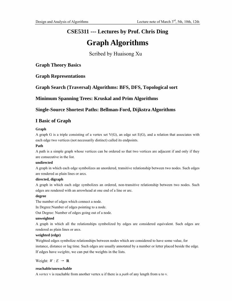
Design and Analysis of Algorithms Lecture note of March 3rd, 5th, 10th, 12th

CSE5311 --- Lectures by Prof. Chris Ding

Graph Algorithms Scribed by Huaisong Xu

Graph Theory Basics

Graph Representations

Graph Search (Traversal) Algorithms: BFS, DFS, Topological sort

Minimum Spanning Trees: Kruskal and Prim Algorithms

Single-Source Shortest Paths: Bellman-Ford, Dijkstra Algorithms

I Basic of Graph Graph A graph G is a triple consisting of a vertex set V(G), an edge set E(G), and a relation that associates with each edge two vertices (not necessarily distinct) called its endpoints. Path A path is a simple graph whose vertices can be ordered so that two vertices are adjacent if and only if they are consecutive in the list. undirected A graph in which each edge symbolizes an unordered, transitive relationship between two nodes. Such edges are rendered as plain lines or arcs. directed, digraph A graph in which each edge symbolizes an ordered, non-transitive relationship between two nodes. Such edges are rendered with an arrowhead at one end of a line or arc. degree The number of edges which connect a node. In Degree:Number of edges pointing to a node. Out Degree: Number of edges going out of a node. unweighted A graph in which all the relationships symbolized by edges are considered equivalent. Such edges are rendered as plain lines or arcs. weighted (edge) Weighted edges symbolize relationships between nodes which are considered to have some value, for instance, distance or lag time. Such edges are usually annotated by a number or letter placed beside the edge. If edges have weights, we can put the weights in the lists.

Weight: w : E → R

reachable/unreachable A vertex v is reachable from another vertex u if there is a path of any length from u to v.


Note: Usually applied only to directed graphs, since any vertex in a connected, undirected graph is reachable from any other vertex.

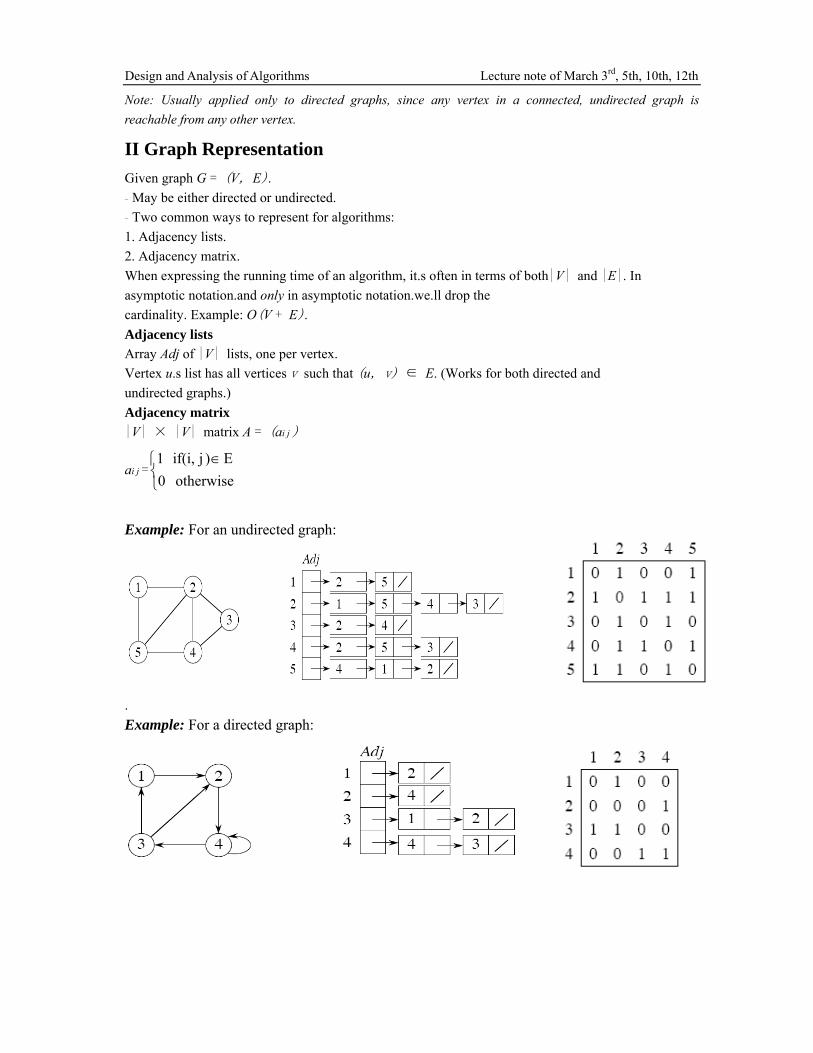
II Graph Representation Given graph G = (V, E). - May be either directed or undirected. - Two common ways to represent for algorithms: 1. Adjacency lists. 2. Adjacency matrix. When expressing the running time of an algorithm, it.s often in terms of both|V| and |E|. In asymptotic notation.and only in asymptotic notation.we.ll drop the cardinality. Example: O(V + E). Adjacency lists Array Adj of |V| lists, one per vertex. Vertex u.s list has all vertices v such that (u, v) ∈ E. (Works for both directed and undirected graphs.) Adjacency matrix |V| × |V| matrix A = (ai j )

ai j =⎩⎨⎧ ∈

otherwise 0E ) j if(i, 1

Example: For an undirected graph:

. Example: For a directed graph:


Counting neighbors A. Counting the number of common neighbors between i,j = # of 2-hop paths between i,j:

)( 2A ij= ∑

=

×n

K 1kjik A A

B. Counting the # of 3-hop paths between i,j:

)( 3A ij= lj

klA××∑ klik A A

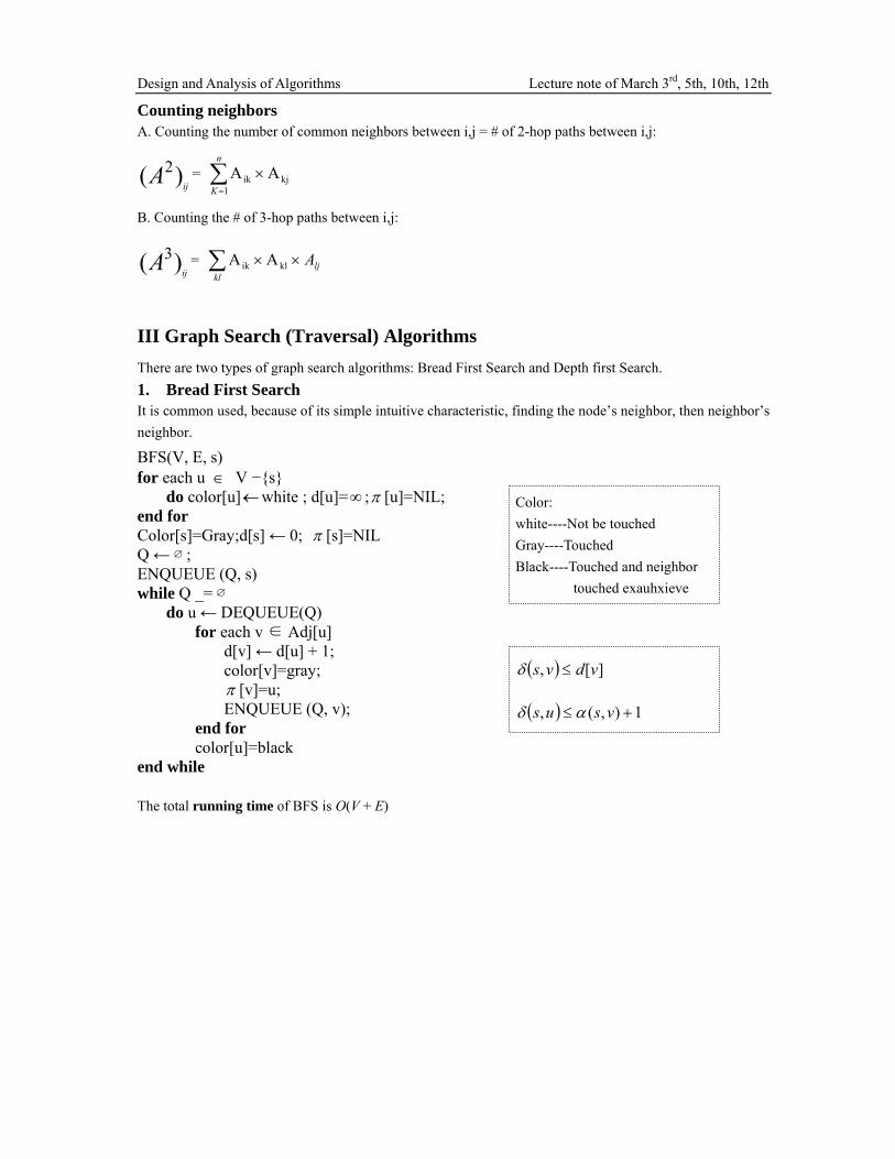
III Graph Search (Traversal) Algorithms There are two types of graph search algorithms: Bread First Search and Depth first Search. 1. Bread First Search It is common used, because of its simple intuitive characteristic, finding the node’s neighbor, then neighbor’s neighbor.

BFS(V, E, s) for each u ∈ V −{s}

do color[u]←white ; d[u]=∞ ;π [u]=NIL; end for Color[s]=Gray;d[s] ← 0; π [s]=NIL Q ← ∅ ; ENQUEUE (Q, s) while Q _= ∅

do u ← DEQUEUE(Q) for each v ∈ Adj[u]

d[v] ← d[u] + 1; color[v]=gray; π [v]=u; ENQUEUE (Q, v);

end for color[u]=black

end while The total running time of BFS is O(V + E)

Color: white----Not be touched Gray----Touched Black----Touched and neighbor

touched exauhxieve

( ) ][, vdvs ≤δ

( ) 1),(, +≤ vsus αδ



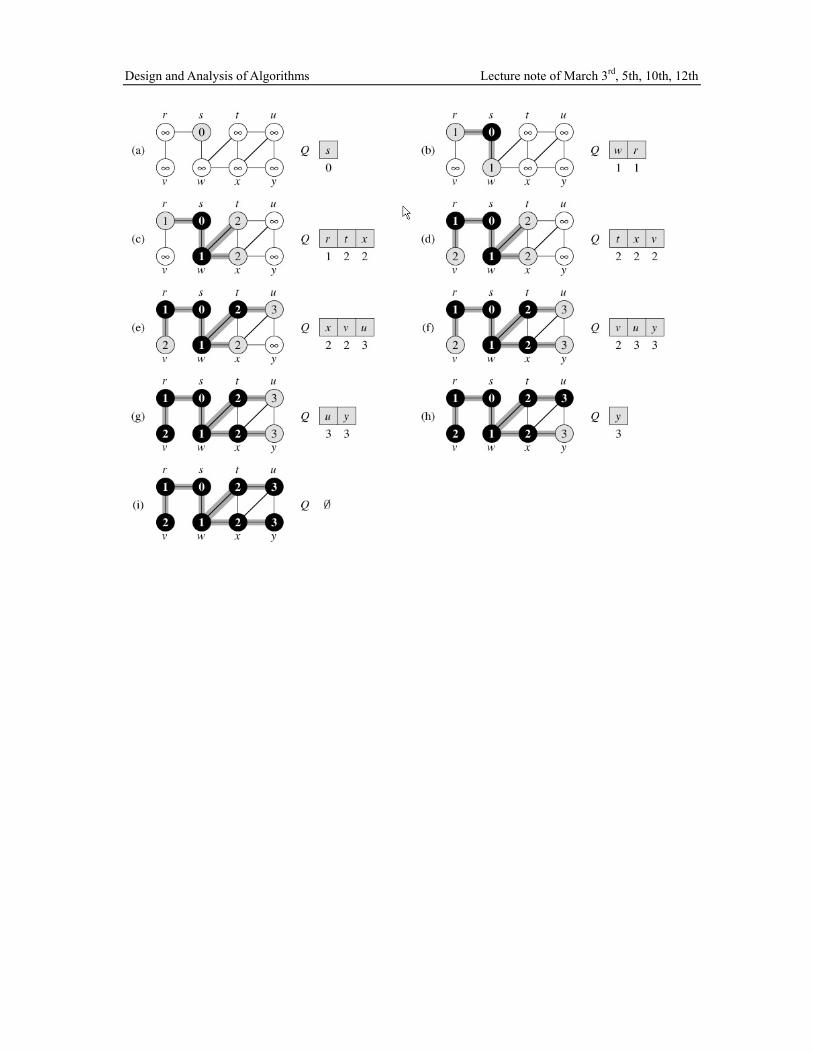
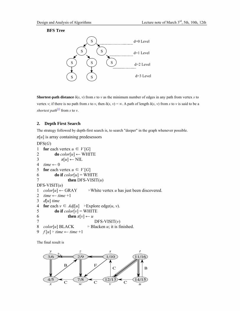
BFS Tree Shortest-path distance δ(s, v) from s to v as the minimum number of edges in any path from vertex s to

vertex v; if there is no path from s to v, then δ(s, v) = ∞. A path of length δ(s, v) from s to v is said to be a

shortest path[1] from s to v.

2. Depth First Search The strategy followed by depth-first search is, to search "deeper" in the graph whenever possible.

π[u] is array containing predesessors DFS(G) 1 for each vertex u ∈ V [G] 2 do color[u] ← WHITE 3 π[u] ← NIL 4 time ← 0 5 for each vertex u ∈ V [G] 6 do if color[u] = WHITE 7 then DFS-VISIT(u) DFS-VISIT(u) 1 color[u] ← GRAY ▹White vertex u has just been discovered. 2 time ← time +1 3 d[u] time 4 for each v ∈ Adj[u] ▹Explore edge(u, v). 5 do if color[v] = WHITE 6 then π[v] ← u 7 DFS-VISIT(v) 8 color[u] BLACK ▹ Blacken u; it is finished. 9 f [u] ▹ time ← time +1 The final result is

S

S S

S S S

S S

d=0 Level

d=1 Level

d=2 Level

d=3 Level


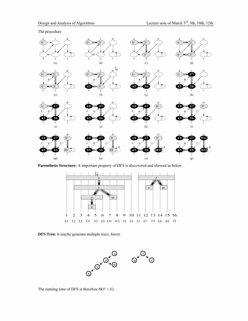
The procedure

Parenthesis Structure: A important property of DFS is discovered and showed as below.

DFS Tree: It maybe generate multiple trees, forest.

The running time of DFS is therefore Θ(V + E).

○s

○z ○y

○u ○v○t

○x ○w


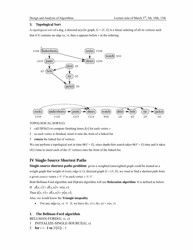
3. Topological Sort A topological sort of a dag, a directed acyclic graph, G = (V, E) is a linear ordering of all its vertices such

that if G contains an edge (u, v), then u appears before v in the ordering.

TOPOLOGICAL-SORT(G)

1 call DFS(G) to compute finishing times f[v] for each vertex v

2 as each vertex is finished, insert it onto the front of a linked list

3 return the linked list of vertices

We can perform a topological sort in time Θ(V + E), since depth-first search takes Θ(V + E) time and it takes

O(1) time to insert each of the |V| vertices onto the front of the linked list.

IV Single-Source Shortest Paths Single-source shortest-paths problem: given a weighted (unweighted graph could be treated as a

weight graph that weight of every edge is 1), directed graph G = (V, E), we want to find a shortest path from

a given source vertex s ∈ V to each vertex v ∈ V .

Both Bellman-Ford algorithm and Dijkstra algorithm will use Relaxation algorithm. It is defined as below:

IF ( ) ( ) ),(,, vuwusdvsd +>

Then d ( ) ( ) ( )vuwusdvs ,,, += ;

Also, we would know the Triangle inequality

• For any edge (u, v) ∈ E, we have δ(s, v) ≤ δ(s, u) + w(u, v)

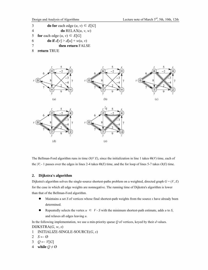
1. The Bellman-Ford algorithm BELLMAN-FORD(G, w, s) 1 INITIALIZE-SINGLE-SOURCE(G, s) 2 for i ← 1 to |V[G]| - 1


3 do for each edge (u, v) ∈ E[G] 4 do RELAX(u, v, w) 5 for each edge (u, v) ∈ E[G] 6 do if d[v] > d[u] + w(u, v) 7 then return FALSE 8 return TRUE

The Bellman-Ford algorithm runs in time O(V E), since the initialization in line 1 takes Θ(V) time, each of

the |V| - 1 passes over the edges in lines 2-4 takes Θ(E) time, and the for loop of lines 5-7 takes O(E) time.

2. Dijkstra's algorithm Dijkstra's algorithm solves the single-source shortest-paths problem on a weighted, directed graph G = (V, E)

for the case in which all edge weights are nonnegative. The running time of Dijkstra's algorithm is lower

than that of the Bellman-Ford algorithm.

Maintains a set S of vertices whose final shortest-path weights from the source s have already been

determined.

Repeatedly selects the vertex u ∈ V - S with the minimum shortest-path estimate, adds u to S,

and relaxes all edges leaving u.

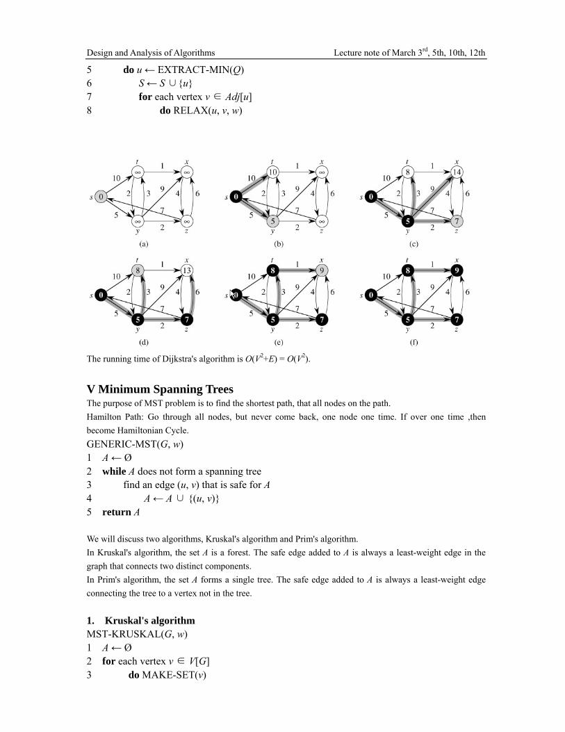
In the following implementation, we use a min-priority queue Q of vertices, keyed by their d values. DIJKSTRA(G, w, s) 1 INITIALIZE-SINGLE-SOURCE(G, s) 2 S ← Ø 3 Q ← V[G] 4 while Q ≠ Ø


5 do u ← EXTRACT-MIN(Q) 6 S ← S ∪{u} 7 for each vertex v ∈ Adj[u] 8 do RELAX(u, v, w)

The running time of Dijkstra's algorithm is O(V2+E) = O(V2).

V Minimum Spanning Trees The purpose of MST problem is to find the shortest path, that all nodes on the path. Hamilton Path: Go through all nodes, but never come back, one node one time. If over one time ,then become Hamiltonian Cycle. GENERIC-MST(G, w) 1 A ← Ø 2 while A does not form a spanning tree 3 find an edge (u, v) that is safe for A 4 A ← A ∪ {(u, v)} 5 return A We will discuss two algorithms, Kruskal's algorithm and Prim's algorithm. In Kruskal's algorithm, the set A is a forest. The safe edge added to A is always a least-weight edge in the graph that connects two distinct components. In Prim's algorithm, the set A forms a single tree. The safe edge added to A is always a least-weight edge connecting the tree to a vertex not in the tree. 1. Kruskal's algorithm MST-KRUSKAL(G, w) 1 A ← Ø 2 for each vertex v ∈ V[G] 3 do MAKE-SET(v)


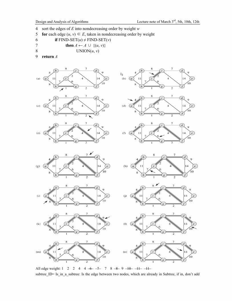
4 sort the edges of E into nondecreasing order by weight w 5 for each edge (u, v) ∈ E, taken in nondecreasing order by weight 6 if FIND-SET(u) ≠ FIND-SET(v) 7 then A ← A ∪ {(u, v)} 8 UNION(u, v) 9 return A

All edge weight: 1 2 2 4 4 6 7 7 8 8 9 10 11 11 subtree_ID= Is_in_a_subtree: Is the edge between two nodes, which are already in Subtree, if in, don’t add


them to subtree, otherwise add them to subtree. Obviously it is not unique.

2. Prim's algorithm

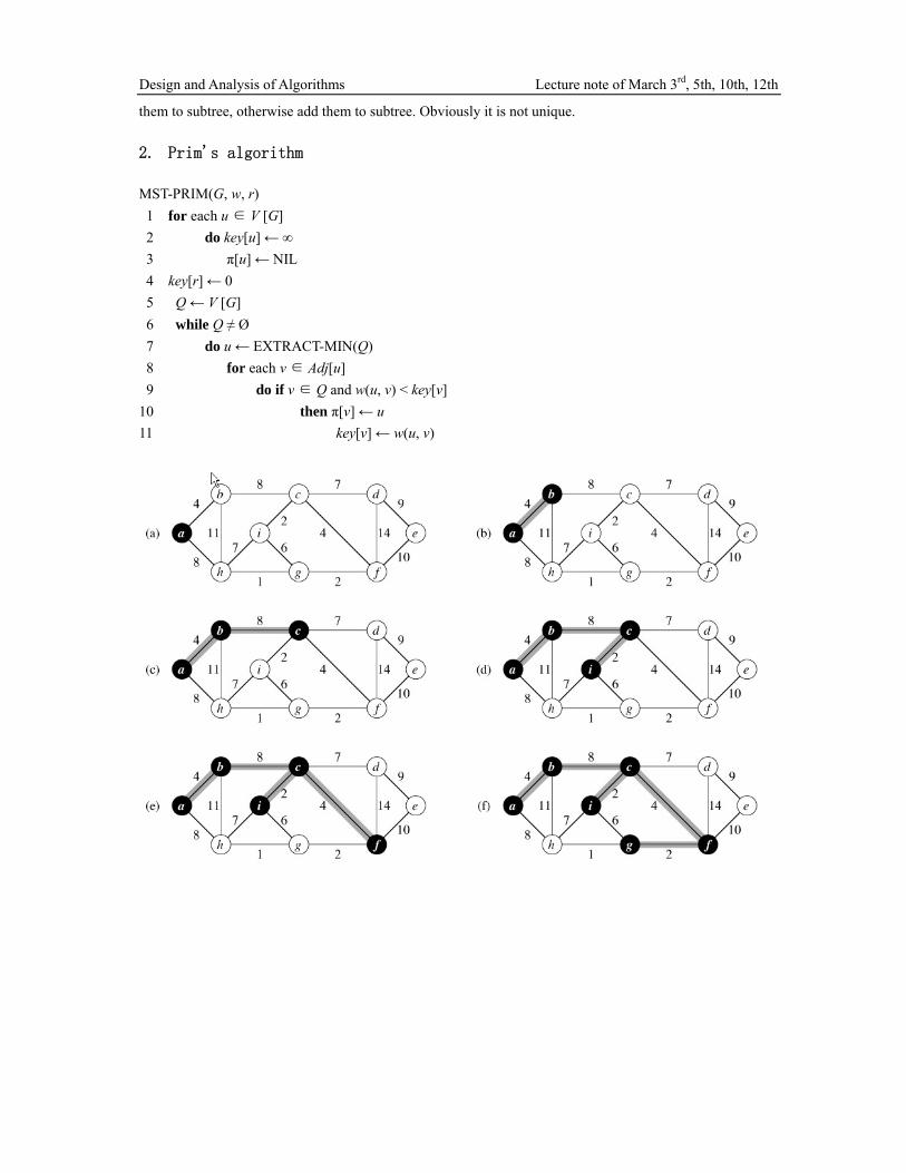
MST-PRIM(G, w, r) 1 for each u ∈ V [G] 2 do key[u] ← ∞ 3 π[u] ← NIL 4 key[r] ← 0 5 Q ← V [G] 6 while Q ≠ Ø 7 do u ← EXTRACT-MIN(Q) 8 for each v ∈ Adj[u] 9 do if v ∈ Q and w(u, v) < key[v] 10 then π[v] ← u 11 key[v] ← w(u, v)


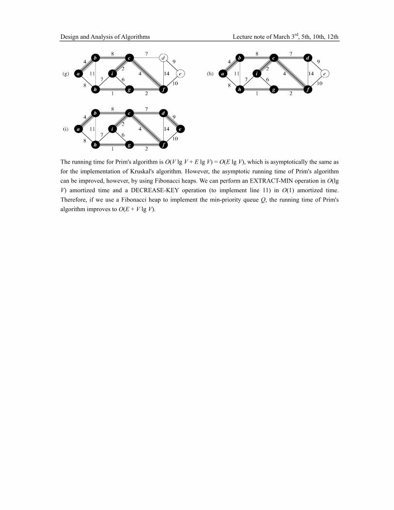
The running time for Prim's algorithm is O(V lg V + E lg V) = O(E lg V), which is asymptotically the same as for the implementation of Kruskal's algorithm. However, the asymptotic running time of Prim's algorithm can be improved, however, by using Fibonacci heaps. We can perform an EXTRACT-MIN operation in O(lg V) amortized time and a DECREASE-KEY operation (to implement line 11) in O(1) amortized time. Therefore, if we use a Fibonacci heap to implement the min-priority queue Q, the running time of Prim's algorithm improves to O(E + V lg V).

Documents

CSE5311 --- Lectures by Prof. Chris Ding Graph Algorithmsranger.uta.edu/~chqding/cse5311/Lectures/GraphTheory.pdf · CSE5311 --- Lectures by Prof. Chris Ding Graph Algorithms Scribed