Lecture Notes: Econ 203 Introductory MicroeconomicsLecture/Chapter 4: Market forces of supply and demand

M. Cary LeaheyManhattan College

Fall 2012

2

Goals

• Explain markets and the underlyig simplifying assumptions• Explain the two blades of the Marshallian scissors• supply and demand• Movements off and along the curves• Market equilibrium and why it holds

3

Markets and assumptions behind them

• Market is a group of buyers and sellers (of a particular product).• Competitive market is one with many (infinite?) number of buyers

and sellers (atomistic). • Price is given so everyone is a price taker.• Homogenous goods (all same in quality).• When in doubt, economists assume perfect (pure) competition.• How realistic: is ice cream really homogeneous?• Assumptions sure make life easier!

4

Demand

• Quantity demanded is the amount of the good buyers are willing and able to purchase.

• Law of demand: quantity demanded is inversely related to the goods (relative) price. If (relative) price goes up, demand goes down.

• The demand schedule: the relationship (table/graph) of quantity demanded and price of the good.

$0.00

$1.00

$2.00

$3.00

$4.00

$5.00

$6.00

0 5 10 15

Price of Javas

Quantity of Javas

Example: Demand Schedule & Curve

Price of javas

Quantity of javas

demanded

$0.00 16

1.00 14

2.00 12

3.00 10

4.00 8

5.00 6

6.00 4

6

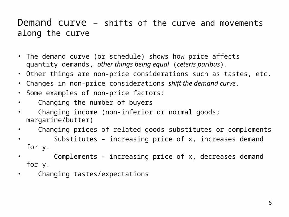
Demand curve – shifts of the curve and movements along the curve

• The demand curve (or schedule) shows how price affects quantity demands, other things being equal (ceteris paribus).

• Other things are non-price considerations such as tastes, etc.• Changes in non-price considerations shift the demand curve.• Some examples of non-price factors:• Changing the number of buyers• Changing income (non-inferior or normal goods; margarine/butter)• Changing prices of related goods-substitutes or complements• Substitutes – increasing price of x, increases demand for y.• Complements - increasing price of x, decreases demand for y.• Changing tastes/expectations

7

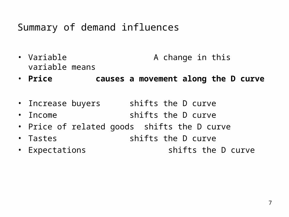
Summary of demand influences

• Variable A change in this variable means• Price causes a movement along the D curve

• Increase buyers shifts the D curve• Income shifts the D curve• Price of related goods shifts the D curve• Tastes shifts the D curve• Expectations shifts the D curve

8

Supply

• Quantity supplied of any good is the amount that sellers willing and able to sell.

• Law of supply: quantity supplied is positively related to the goods (relative) price. If (relative) price goes up, supply goes up.

• The supply schedule: the relationship (table/graph) of quantity supplied and price of the good.

$0.00

$1.00

$2.00

$3.00

$4.00

$5.00

$6.00

0 5 10 15

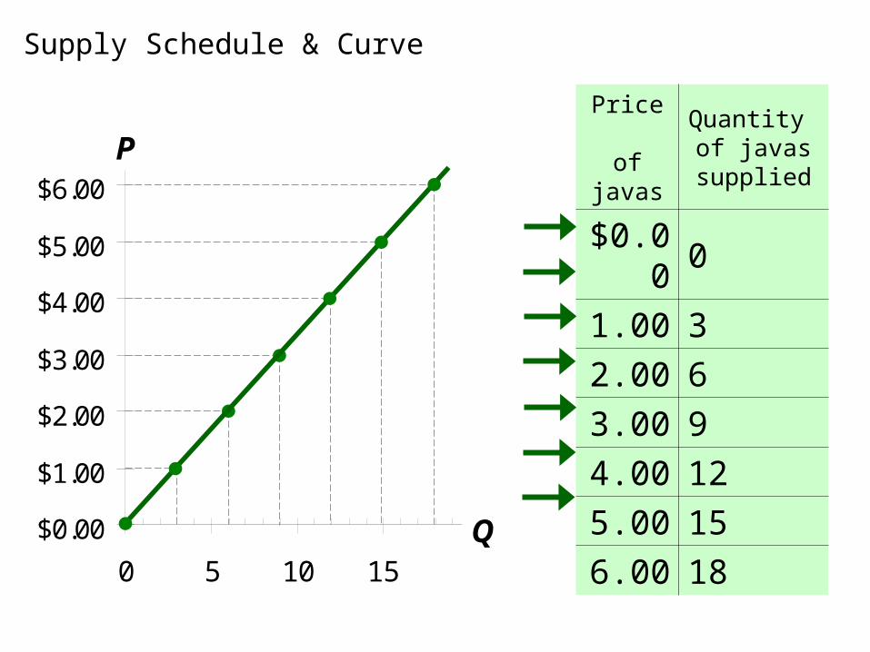
Supply Schedule & Curve

Price of javas

Quantity of javas supplied

$0.00 0

1.00 3

2.00 6

3.00 9

4.00 12

5.00 15

6.00 18

P

Q

10

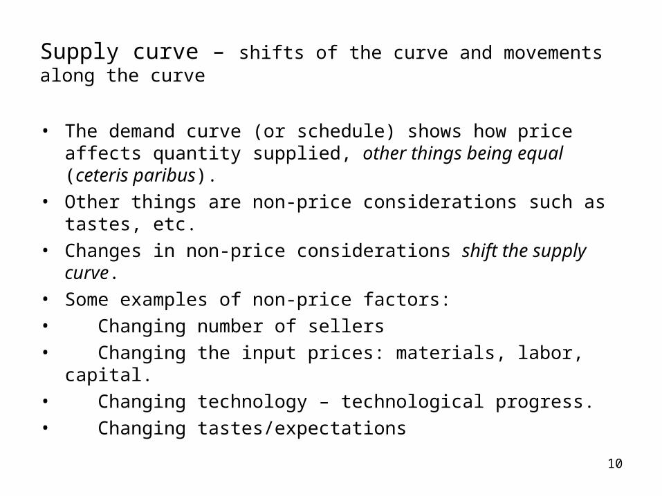
Supply curve – shifts of the curve and movements along the curve

• The demand curve (or schedule) shows how price affects quantity supplied, other things being equal (ceteris paribus).

• Other things are non-price considerations such as tastes, etc.• Changes in non-price considerations shift the supply curve.• Some examples of non-price factors:• Changing number of sellers • Changing the input prices: materials, labor, capital.• Changing technology – technological progress.• Changing tastes/expectations

11

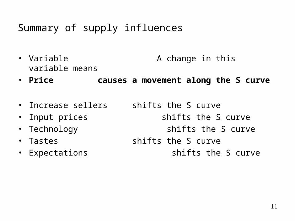
Summary of supply influences

• Variable A change in this variable means• Price causes a movement along the S curve

• Increase sellers shifts the S curve• Input prices shifts the S curve• Technology shifts the S curve• Tastes shifts the S curve• Expectations shifts the S curve

12

Equilibrium – supply and demand together

• Equilibrium has been reached when quantity demanded and supplied are equal.

• Equilibrium price is the price that equates demand and supply.• Almost a tautology as movements along the two curves eventually

returns to equilibrium, after trial and error

$0.00

$1.00

$2.00

$3.00

$4.00

$5.00

$6.00

0 5 10 15 20 25 30 35

P

Q

D S

Surplus (excess supply), when quantity supplied is greater than quantity demanded

SurplusExample: If P = $5,

then QD = 9 javas

and QS = 25 javas

resulting in a surplus of 16 javas

$0.00

$1.00

$2.00

$3.00

$4.00

$5.00

$6.00

0 5 10 15 20 25 30 35

P

Q

D S

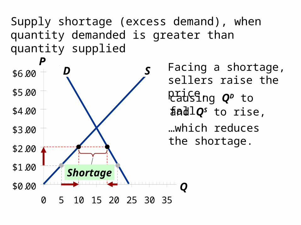
Supply shortage (excess demand), when quantity demanded is greater than quantity supplied

Facing a shortage, sellers raise the price,

causing QD to fall

…which reduces the shortage.

and QS to rise,

Shortage

15

How to analyze changes in market equilibrium

• Decide if event shifts S, D curve or both• Decide which direction the curve(s) shift• Use equilibrium diagram to see how shift changes P and Q.• The ultimate changes in P and Q depend on the relative slopes of

the curves and the elasticity (sensitivity) of supply and demand to price, something we will look at later in the course.

© 2012 Cengage Learning. All Rights Reserved. May not be copied, scanned, or duplicated, in whole or in part, except for use as permitted in a license distributed with a certain product or service or otherwise on a password-protected website for classroom use.

1616

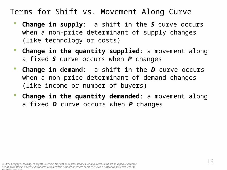
Terms for Shift vs. Movement Along Curve

Change in supply: a shift in the S curve occurs when a non-price determinant of supply changes (like technology or costs)

Change in the quantity supplied: a movement along a fixed S curve occurs when P changes

Change in demand: a shift in the D curve occurs when a non-price determinant of demand changes (like income or number of buyers)

Change in the quantity demanded: a movement along a fixed D curve occurs when P changes

17

How prices allocate resources

• In market economies, prices adjust supply and demand.• Prices are signals that guide economic decisionmaking and allocate

(scarce) resources.

18

Summary

• Competitive (pure/atomistic) market – many buyers and sellers, each of whom has no influence on prices. They are price takers.

• Supply and demand curves are simplifying tools (models) used to study markets.

• Demand curve is downward sloping, as price is inversely related to quantity demanded.

• Supply curve is upward sloping, as prices in positively related to quantity supplied.

• Prices move along the curve; other factors shift the curves.• The intersection of supply and demand determines the equilibrium

price.• To analyze impacts on markets, see if the example studied sifts

supply, demand or both. Examine the relative shifts in the curve and where the new equilibrium plays out and is compared to the old one.