LECTURE 8Stabilization policy

Øystein Børsum

7th March 2006

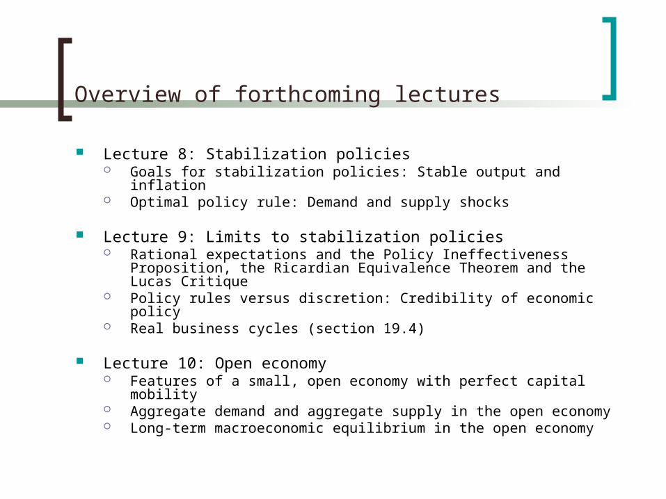
Overview of forthcoming lectures

Lecture 8: Stabilization policies Goals for stabilization policies: Stable output and inflation Optimal policy rule: Demand and supply shocks

Lecture 9: Limits to stabilization policies Rational expectations and the Policy Ineffectiveness Proposition,

the Ricardian Equivalence Theorem and the Lucas Critique Policy rules versus discretion: Credibility of economic policy Real business cycles (section 19.4)

Lecture 10: Open economy Features of a small, open economy with perfect capital mobility Aggregate demand and aggregate supply in the open economy Long-term macroeconomic equilibrium in the open economy

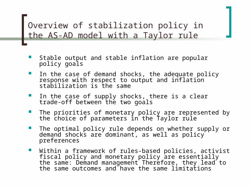
Overview of stabilization policy in the AS-AD model with a Taylor rule

Stable output and stable inflation are popular policy goals

In the case of demand shocks, the adequate policy response with respect to output and inflation stabilization is the same

In the case of supply shocks, there is a clear trade-off between the two goals

The priorities of monetary policy are represented by the choice of parameters in the Taylor rule

The optimal policy rule depends on whether supply or demand shocks are dominant, as well as policy preferences

Within a framework of rules-based policies, activist fiscal policy and monetary policy are essentially the same: Demand management Therefore, they lead to the same outcomes and have the same limitations

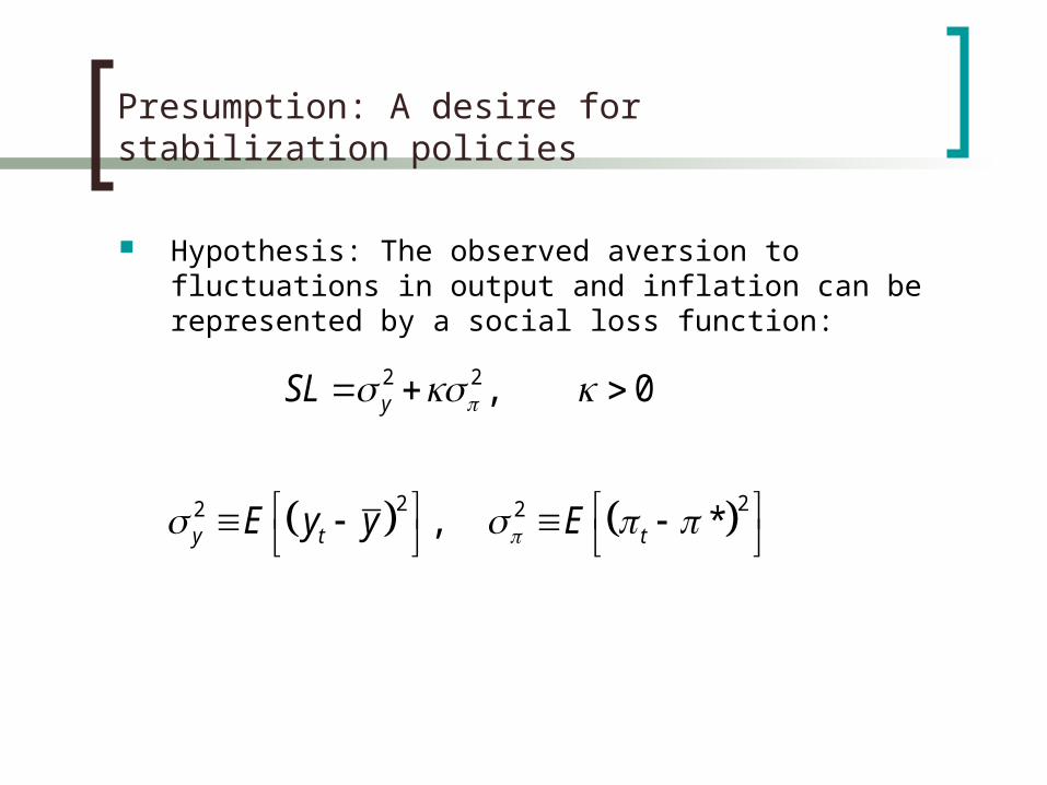
Presumption: A desire for stabilization policies

Hypothesis: The observed aversion to fluctuations in output and inflation can be represented by a social loss function:

2 2

2 22 2

, 0

, *

y

y t t

SL

E y y E

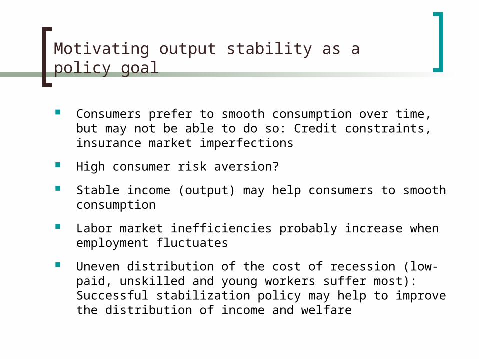
Motivating output stability as a policy goal

Consumers prefer to smooth consumption over time, but may not be able to do so: Credit constraints, insurance market imperfections

High consumer risk aversion?

Stable income (output) may help consumers to smooth consumption

Labor market inefficiencies probably increase when employment fluctuates

Uneven distribution of the cost of recession (low-paid, unskilled and young workers suffer most): Successful stabilization policy may help to improve the distribution of income and welfare

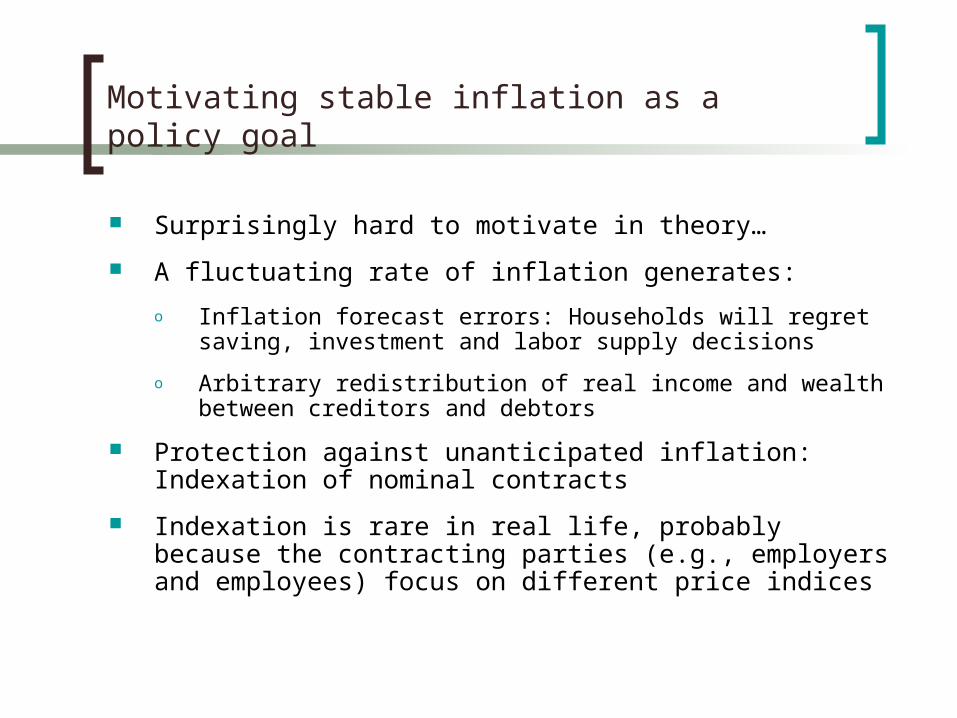
Motivating stable inflation as a policy goal

Surprisingly hard to motivate in theory…

A fluctuating rate of inflation generates:

o Inflation forecast errors: Households will regret saving, investment and labor supply decisions

o Arbitrary redistribution of real income and wealth between creditors and debtors

Protection against unanticipated inflation: Indexation of nominal contracts

Indexation is rare in real life, probably because the contracting parties (e.g., employers and employees) focus on different price indices

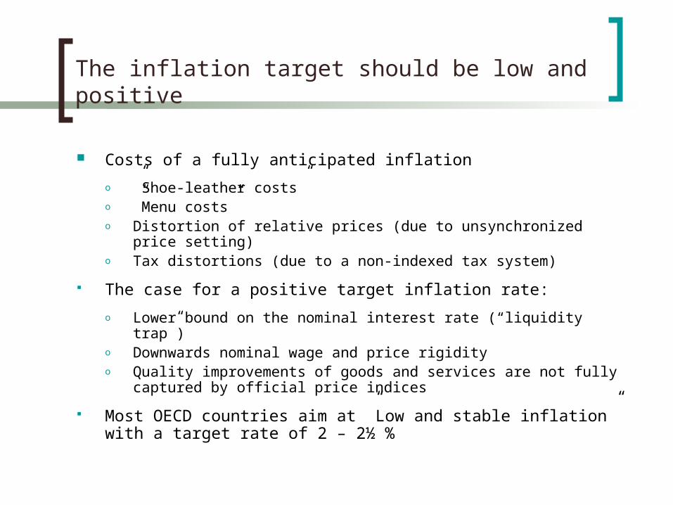
The inflation target should be low and positive

Costs of a fully anticipated inflation

o ”Shoe-leather costs” o ”Menu costs” o Distortion of relative prices (due to unsynchronized price setting)o Tax distortions (due to a non-indexed tax system)

The case for a positive target inflation rate:

o Lower bound on the nominal interest rate (“liquidity trap”)o Downwards nominal wage and price rigidityo Quality improvements of goods and services are not fully

captured by official price indices

Most OECD countries aim at ”Low and stable inflation” with a target rate of 2 – 2½ %

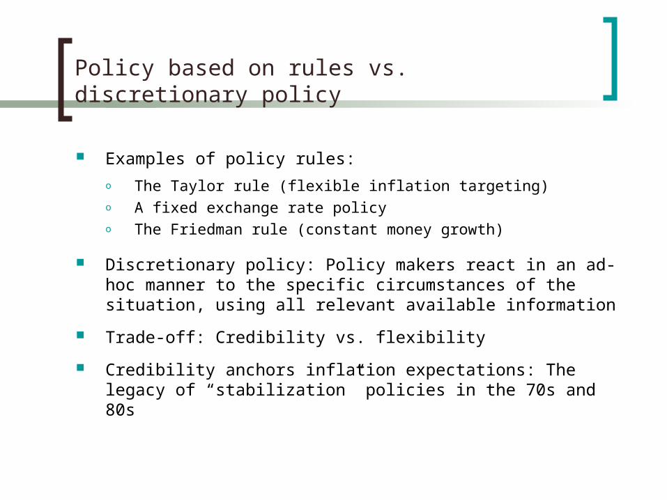
Policy based on rules vs. discretionary policy

Examples of policy rules:

o The Taylor rule (flexible inflation targeting)o A fixed exchange rate policy o The Friedman rule (constant money growth)

Discretionary policy: Policy makers react in an ad-hoc manner to the specific circumstances of the situation, using all relevant available information

Trade-off: Credibility vs. flexibility

Credibility anchors inflation expectations: The legacy of “stabilization” policies in the 70s and 80s

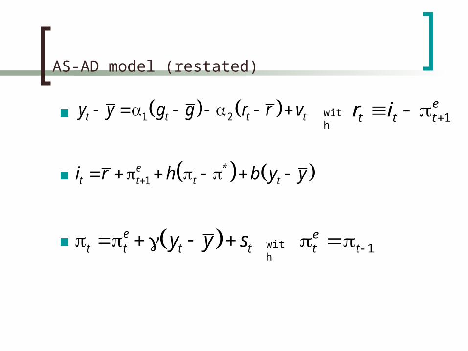
AS-AD model (restated)

1e *

t t t ti r h b y y

1 2t t t ty y g g r r v 1e

t t tr i with

et t t ty y s 1

et t with

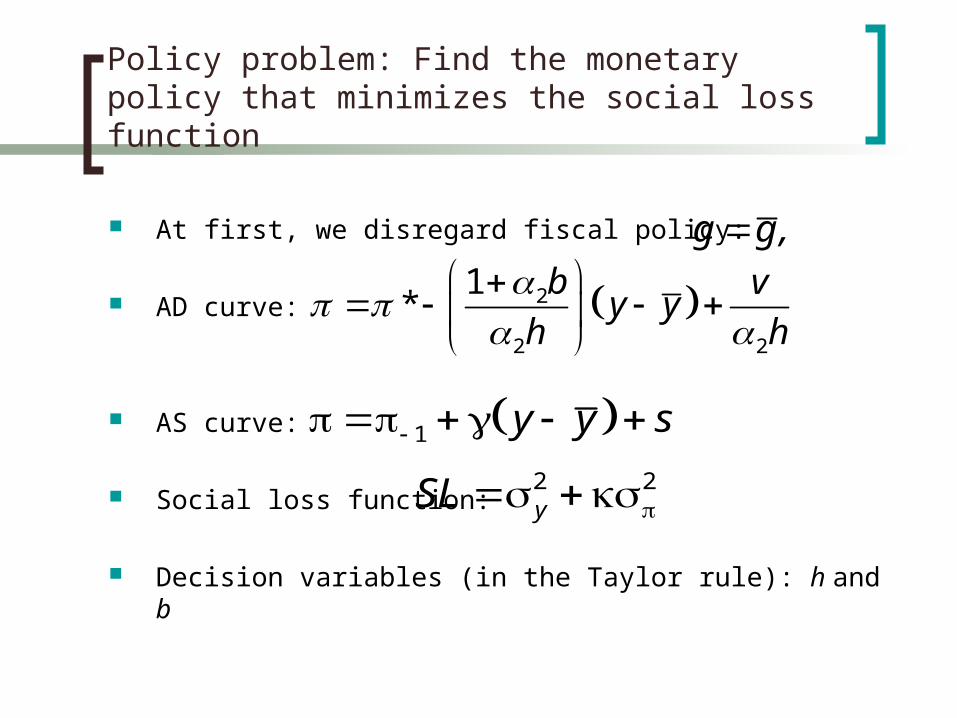
Policy problem: Find the monetary policy that minimizes the social loss function

At first, we disregard fiscal policy:

AD curve:

AS curve:

Social loss function:

Decision variables (in the Taylor rule): h and b

g g ,

2

2 2

1*

b vy y

h h

1 y y s 2 2ySL

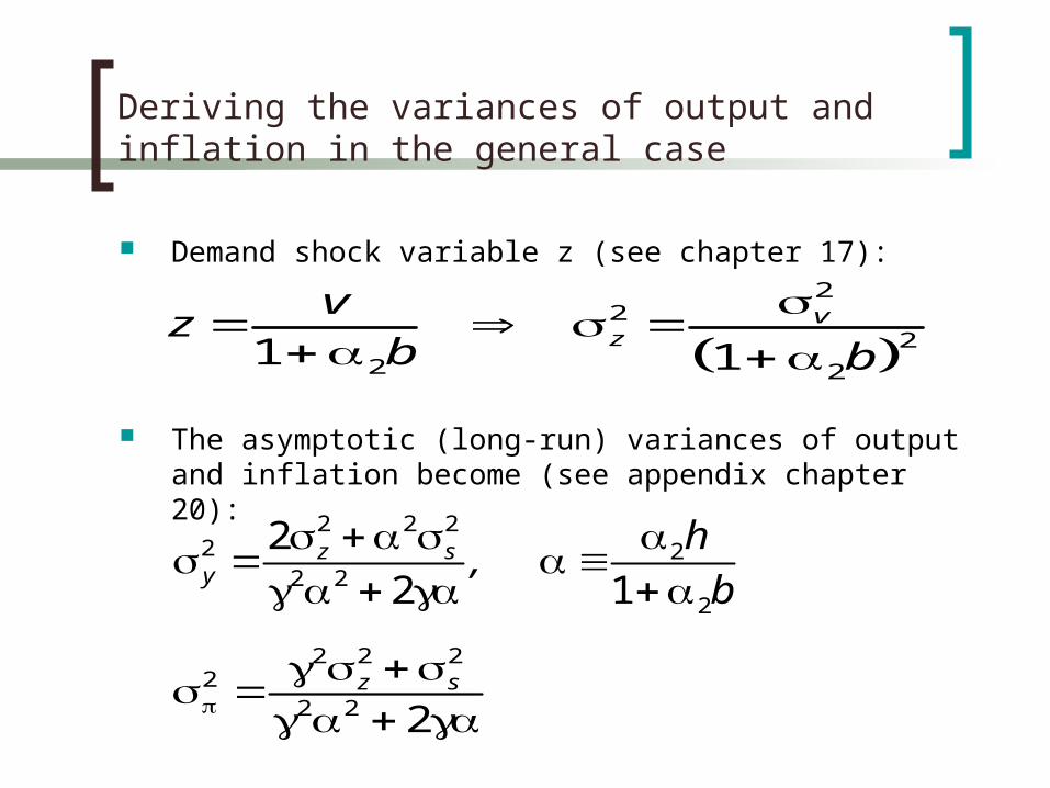
Deriving the variances of output and inflation in the general case

Demand shock variable z (see chapter 17):

The asymptotic (long-run) variances of output and inflation become (see appendix chapter 20):

22

22 2

1 1

vz

vz

b b

2 2 22 2

2 22

2

2 1z s

y

h,

b

2 2 2

22 2 2

z s

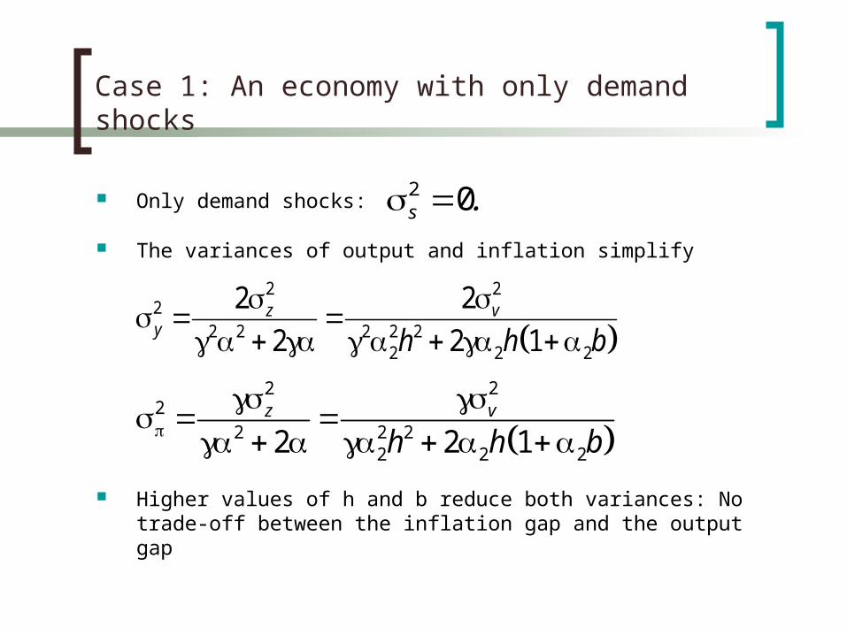
Case 1: An economy with only demand shocks

Only demand shocks:

The variances of output and inflation simplify

Higher values of h and b reduce both variances: No trade-off between the inflation gap and the output gap

2 0s .

22

22 2 2 2 2

2 2 2

22

2 2 1vz

y h h b

22

22 2 2

2 2 22 2 1vz

h h b

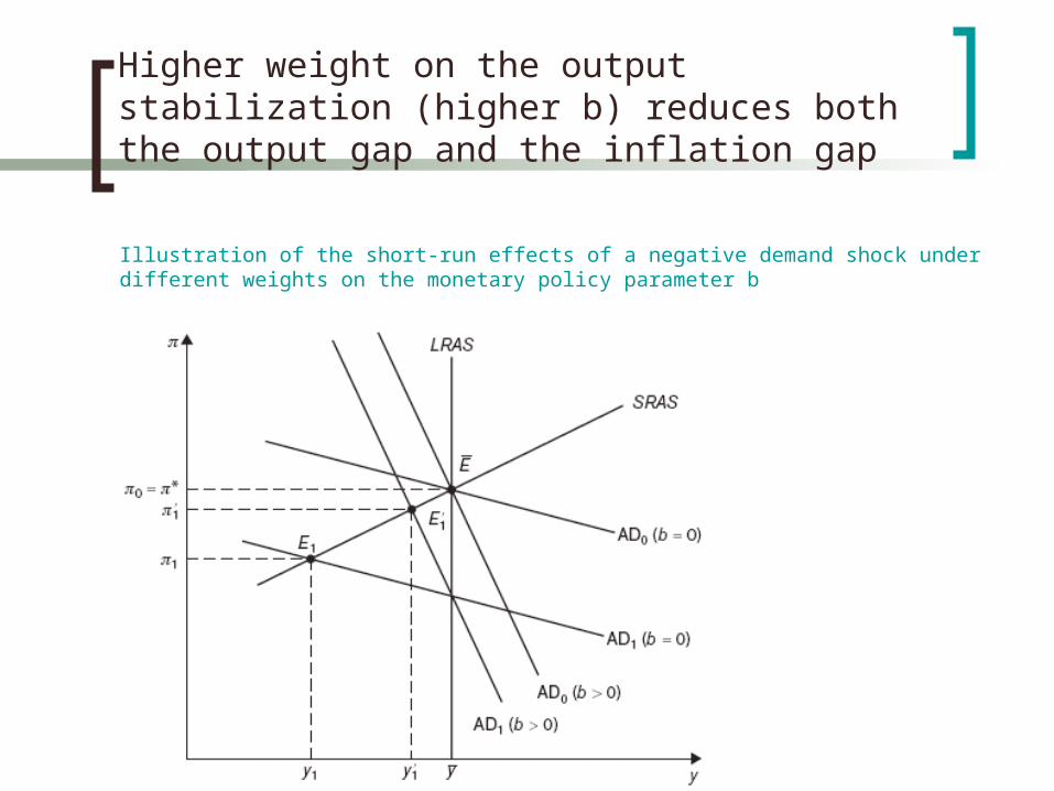
Higher weight on the output stabilization (higher b) reduces both the output gap and the inflation gap

Illustration of the short-run effects of a negative demand shock under different weights on the monetary policy parameter b

Conclusion: No policy trade-off in an economy with only demand shocks

The central bank should react to demand shocks by pursuing a countercyclical monetary policy (b > 0).

There is no trade-off between stabilizing output and stabilizing inflation when business cycles are driven by demand shocks.

When faced with demand shocks, the central bank should react as strongly as possible to the output and inflation gaps.

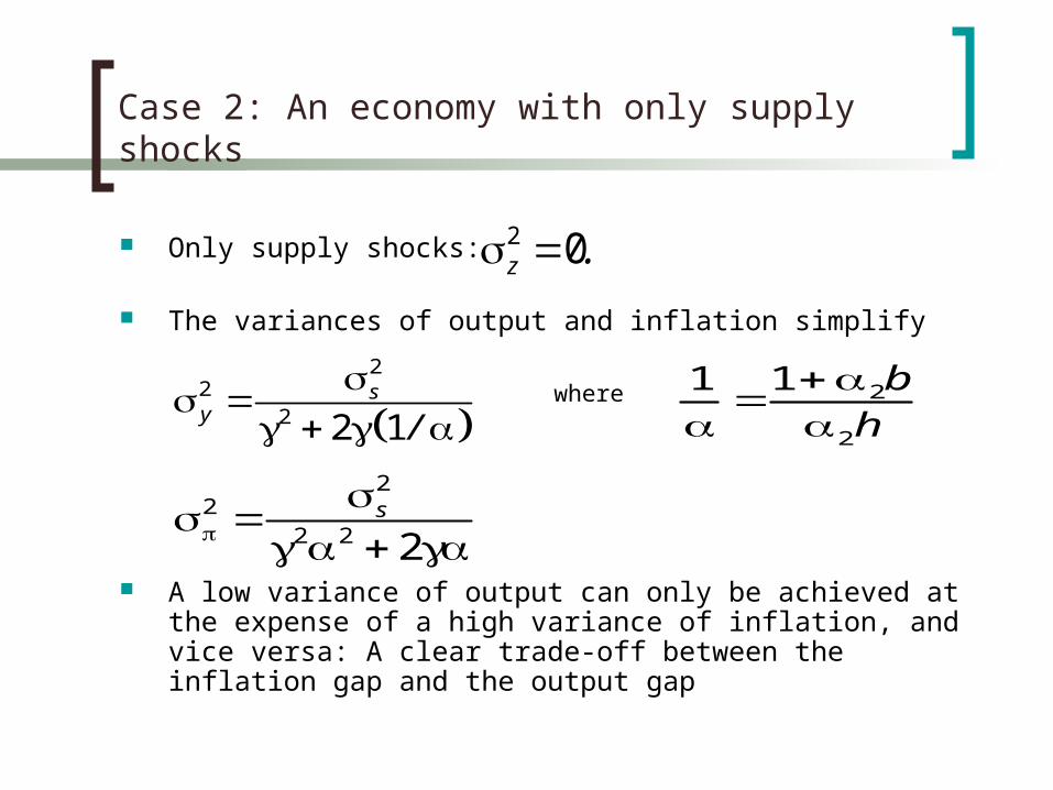
Case 2: An economy with only supply shocks

Only supply shocks:

The variances of output and inflation simplify

A low variance of output can only be achieved at the expense of a high variance of inflation, and vice versa: A clear trade-off between the inflation gap and the output gap

2 0z .

2

22 2 1

sy /

2

22 2 2

s

2

2

1 1 b

h

where

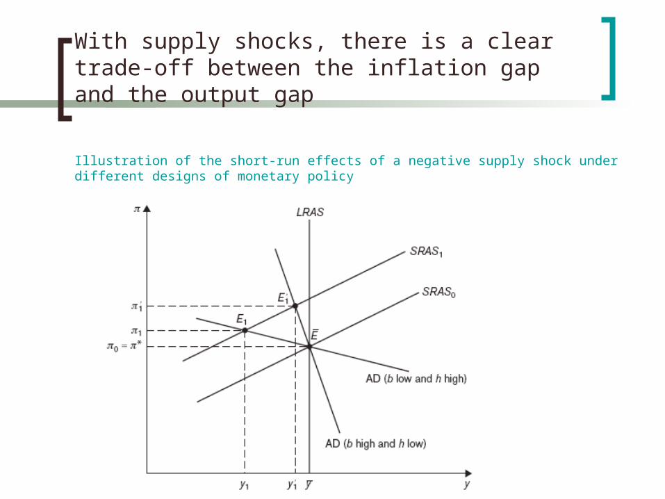
With supply shocks, there is a clear trade-off between the inflation gap and the output gap

Illustration of the short-run effects of a negative supply shock under different designs of monetary policy

Conclusion: Clear policy trade-off in an economy with only supply shocks

If policy makers primarily seek to stabilize output, b should be positive and high (countercyclical policy) and h should be close to zero so that the AD curve becomes steep.

If policy makers primarily seek to stabilize inflation, b should be negative (procyclical policy) and h should be high so that the AD curve becomes flat.

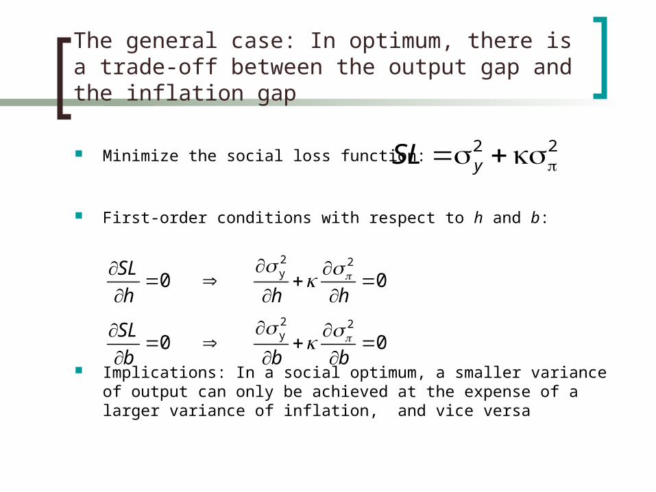
The general case: In optimum, there is a trade-off between the output gap and the inflation gap

Minimize the social loss function:

First-order conditions with respect to h and b:

Implications: In a social optimum, a smaller variance of output can only be achieved at the expense of a larger variance of inflation, and vice versa

2 2ySL

2 2y0 0

SL

h h h

2 2y0 0

SL

b b b

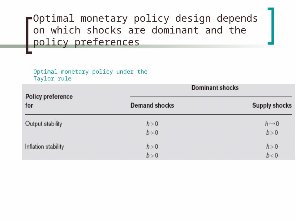
Optimal monetary policy design depends on which shocks are dominant and the policy preferences

Optimal monetary policy under the Taylor rule

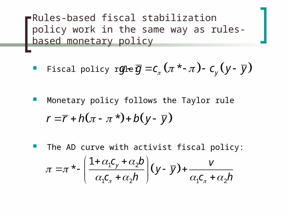
Rules-based fiscal stabilization policy work in the same way as rules-based monetary policy

Fiscal policy rule:

Monetary policy follows the Taylor rule

The AD curve with activist fiscal policy:

* yg g c c y y

*r r h b y y

1 2

1 2 1 2

1* yc b v

y yc h c h

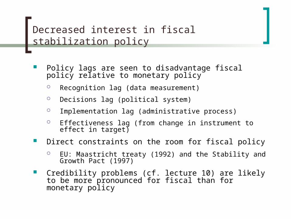
Decreased interest in fiscal stabilization policy

Policy lags are seen to disadvantage fiscal policy relative to monetary policy Recognition lag (data measurement)

Decisions lag (political system)

Implementation lag (administrative process)

Effectiveness lag (from change in instrument to effect in target)

Direct constraints on the room for fiscal policy EU: Maastricht treaty (1992) and the Stability and Growth Pact

(1997)

Credibility problems (cf. lecture 10) are likely to be more pronounced for fiscal than for monetary policy