Lecture 8: Cost of capital. Financial modeling of a project

Lecture 8: Cost of capital. Financial modeling of a

project

www.finint.ase.ro

Phases in Financial Modeling of a project

2

1. Initial investment cost

2. Capital structure

3. Optimal financing alternative

4. Financing plan. Evaluating the WACC

5. Evaluating project’s cash flows

6. Evaluating the financial performance of the project

7. Sensitivity analysis

8. Break – Even Point Analysis

Step 1: Evaluating initial investment

3

Total cost of investment project should include:

Cost with land

Buildings, production facilities;

Capital Equipments

Installment costs

Testing the equipments

Permits, authorizations

Additional infrastructure

Overheads (10%)

Evaluating an investment project (example)

4

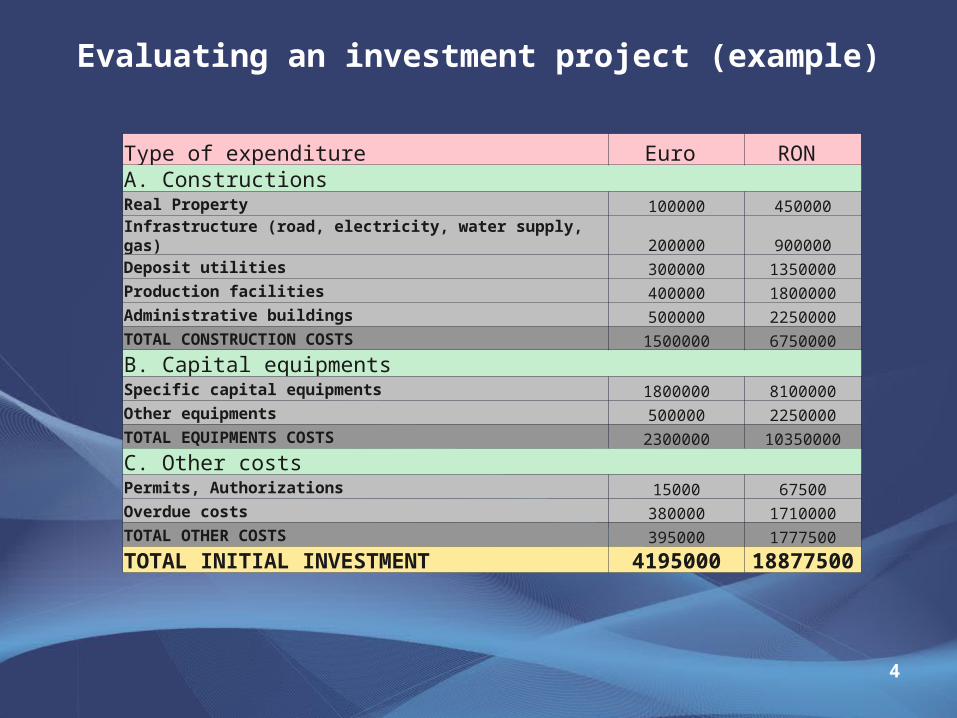
Type of expenditure Euro RON A. Constructions Real Property 100000 450000

Infrastructure (road, electricity, water supply, gas) 200000 900000Deposit utilities 300000 1350000Production facilities 400000 1800000Administrative buildings 500000 2250000TOTAL CONSTRUCTION COSTS 1500000 6750000

B. Capital equipments Specific capital equipments 1800000 8100000Other equipments 500000 2250000TOTAL EQUIPMENTS COSTS 2300000 10350000

C. Other costs Permits, Authorizations 15000 67500Overdue costs 380000 1710000TOTAL OTHER COSTS 395000 1777500

TOTAL INITIAL INVESTMENT 4195000 18877500

Step 2: Optimal capital structure

5

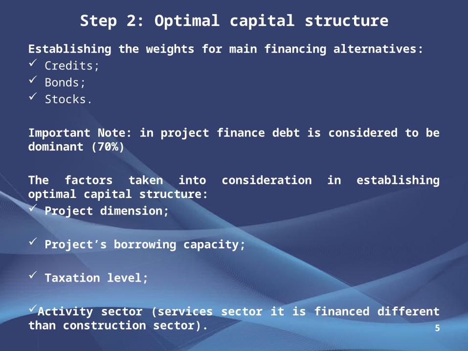
Establishing the weights for main financing alternatives: Credits; Bonds; Stocks.

Important Note: in project finance debt is considered to be dominant (70%)

The factors taken into consideration in establishing optimal capital structure: Project dimension;

Project’s borrowing capacity;

Taxation level;

Activity sector (services sector it is financed different than construction sector).

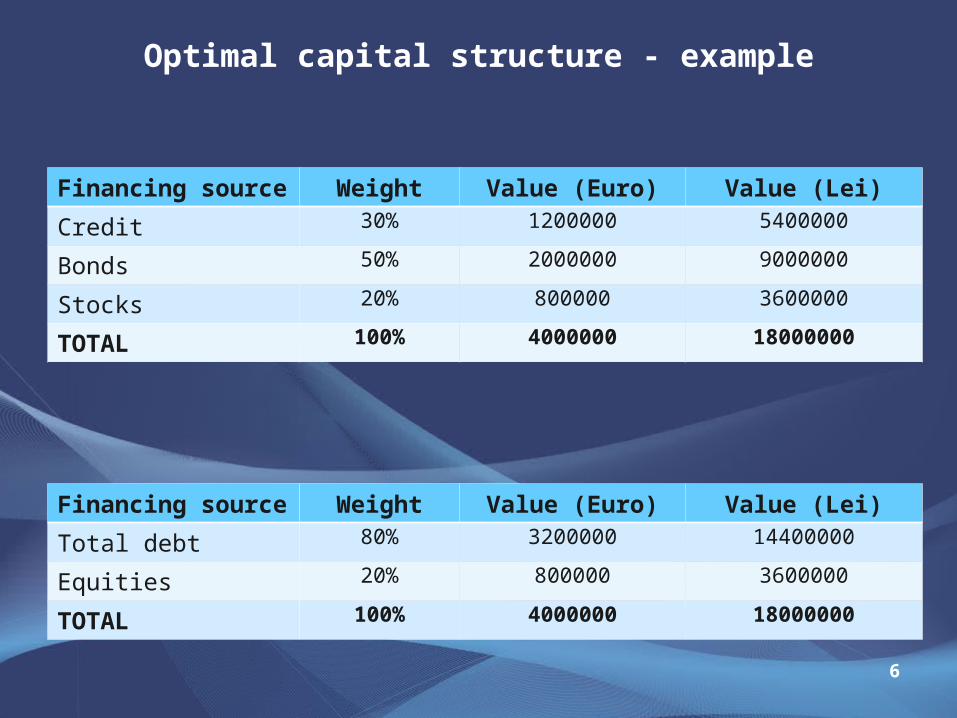
Optimal capital structure - example

6

Financing source Weight Value (Euro) Value (Lei)

Credit 30% 1200000 5400000

Bonds 50% 2000000 9000000

Stocks 20% 800000 3600000

TOTAL 100% 4000000 18000000

Financing source Weight Value (Euro) Value (Lei)

Total debt 80% 3200000 14400000

Equities 20% 800000 3600000

TOTAL 100% 4000000 18000000

Step 3: Optimal financing alternative

7

• This phase supposes to chose among different offers for each financing source (credit, bonds, equities);

• Selection is based on the characteristics of each offer (interest rate, reimbursement program, maturity, other facilities);

• Criteria used to compare different financing alternatives:

– NPV criterion

– IRR criterion

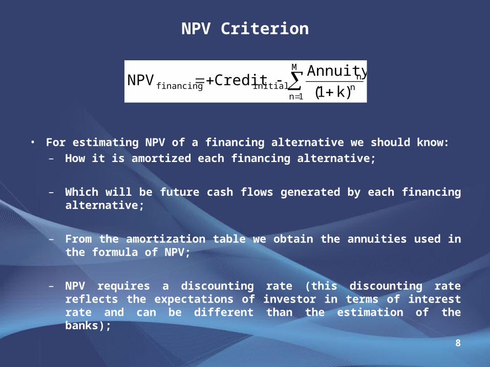
NPV Criterion

8

• For estimating NPV of a financing alternative we should know:

– How it is amortized each financing alternative;

– Which will be future cash flows generated by each financing alternative;

– From the amortization table we obtain the annuities used in the formula of NPV;

– NPV requires a discounting rate (this discounting rate reflects the expectations of investor in terms of interest rate and can be different than the estimation of the banks);

M

1nnn

initialfinancing )k1(

AnnuityCreditNPV

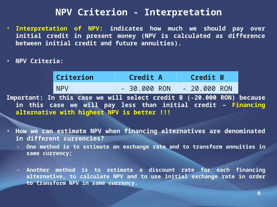
NPV Criterion - Interpretation

9

• Interpretation of NPV: indicates how much we should pay over initial credit in present money (NPV is calculated as difference between initial credit and future annuities).

• NPV Criteria:

Important: In this case we will select credit B (-20.000 RON) because in this case we will pay less than initial credit – Financing alternative with highest NPV is better !!!

• How we can estimate NPV when financing alternatives are denominated in different currencies?– One method is to estimate an exchange rate and to transform annuities in same

currency;

– Another method is to estimate a discount rate for each financing alternative, to calculate NPV and to use initial exchange rate in order to transform NPV in same currency.

Criterion Credit A Credit B

NPV - 30.000 RON - 20.000 RON

IRR Criterion

10

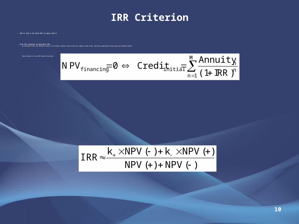
• IRR is that k for which NPV is equal with 0:

• From this equation we determine IRR:– By successive trials (for different values of k we obtain a positive value of NPV and a negative value of NPV ) and than we approximate IRR by using the following formula:

– Other solution is to use IRR function from Excel .

M

1nnn

initialfinancing )I(1Annuity

Credit NRR

0PV

)(NPV)(NPV

)(NPVk)(NPVkIRR

IRR Criterion - interpretation

11

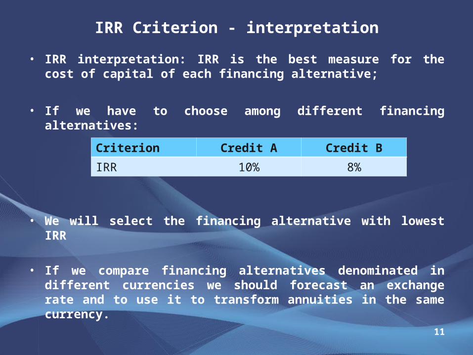
• IRR interpretation: IRR is the best measure for the cost of capital of each financing alternative;

• If we have to choose among different financing alternatives:

• We will select the financing alternative with lowest IRR

• If we compare financing alternatives denominated in different currencies we should forecast an exchange rate and to use it to transform annuities in the same currency.

Criterion Credit A Credit B

IRR 10% 8%

IRR and NPV Criteria to select optimal financing alternative - conclusions

12

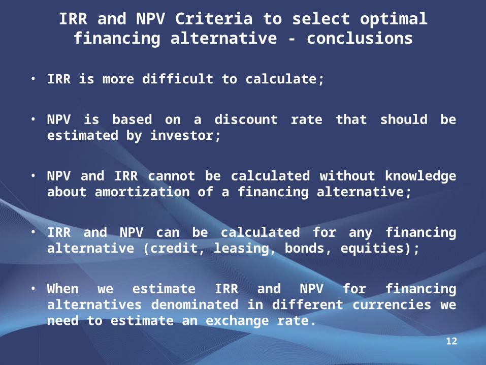
• IRR is more difficult to calculate;

• NPV is based on a discount rate that should be estimated by investor;

• NPV and IRR cannot be calculated without knowledge about amortization of a financing alternative;

• IRR and NPV can be calculated for any financing alternative (credit, leasing, bonds, equities);

• When we estimate IRR and NPV for financing alternatives denominated in different currencies we need to estimate an exchange rate.

13

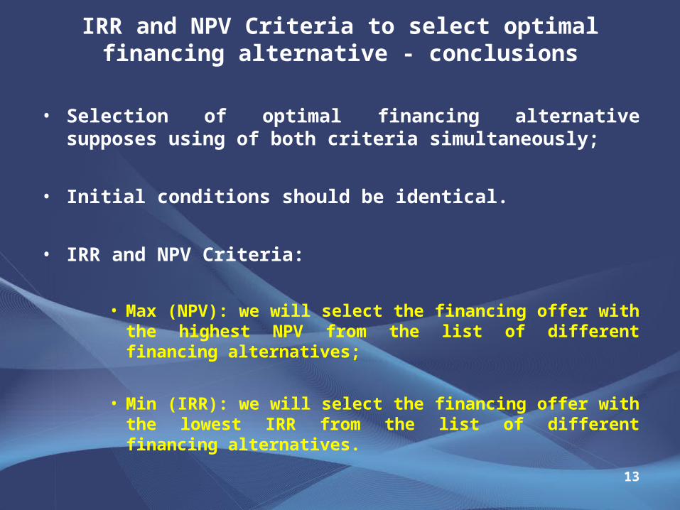
• Selection of optimal financing alternative supposes using of both criteria simultaneously;

• Initial conditions should be identical.

• IRR and NPV Criteria:

• Max (NPV): we will select the financing offer with the highest NPV from the list of different financing alternatives;

• Min (IRR): we will select the financing offer with the lowest IRR from the list of different financing alternatives.

IRR and NPV Criteria to select optimal financing alternative - conclusions

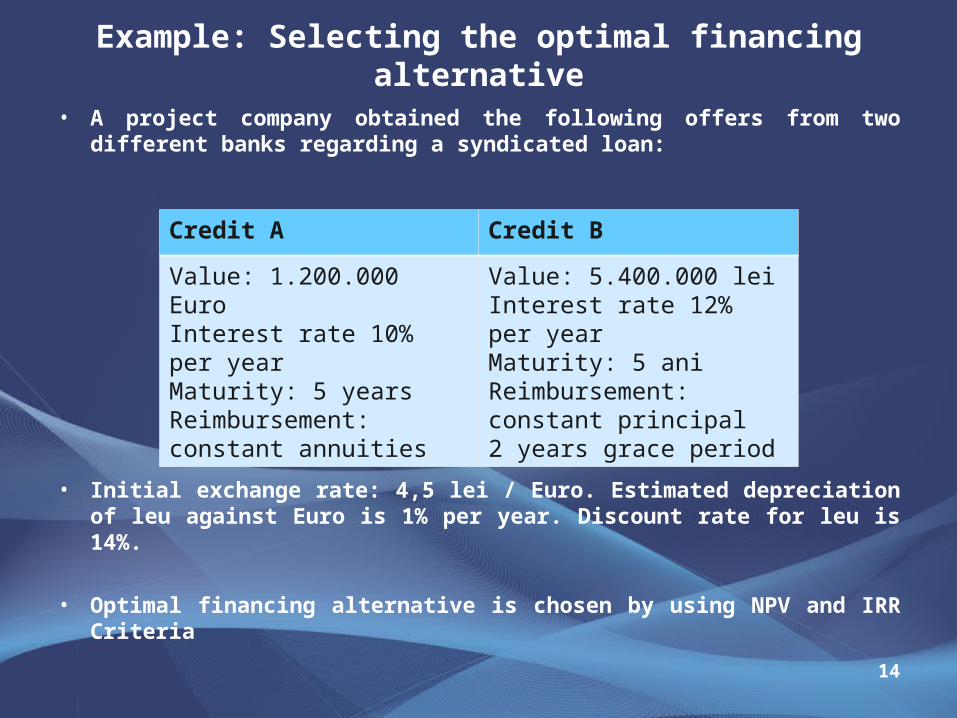
Example: Selecting the optimal financing alternative

14

• A project company obtained the following offers from two different banks regarding a syndicated loan:

• Initial exchange rate: 4,5 lei / Euro. Estimated depreciation of leu against Euro is 1% per year. Discount rate for leu is 14%.

• Optimal financing alternative is chosen by using NPV and IRR Criteria

Credit A Credit B

Value: 1.200.000 EuroInterest rate 10% per yearMaturity: 5 yearsReimbursement: constant annuities

Value: 5.400.000 leiInterest rate 12% per yearMaturity: 5 aniReimbursement: constant principal2 years grace period

Financing plan

15

• Is a synthesis of all financing alternatives involved in project’s financing;

• Shows the financing conditions associated to each financing alternative;

• Reflects the cost of capital associated to each financing alternative (IRR for all of them);

• It is used to determine the cash flows generated by each financing alternative;

• It is used to calculate WACC for project financing plan;

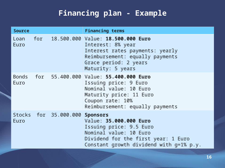
Financing plan - Example

16

Source Financing terms

Loan for 18.500.000 Euro Value: 18.500.000 EuroInterest: 8% yearInterest rates payments: yearlyReimbursement: equally paymentsGrace period: 2 yearsMaturity: 5 years

Bonds for 55.400.000 Euro Value: 55.400.000 EuroIssuing price: 9 EuroNominal value: 10 EuroMaturity price: 11 EuroCoupon rate: 10%Reimbursement: equally payments

Stocks for 35.000.000 Euro SponsorsValue: 35.000.000 EuroIssuing price: 9.5 EuroNominal value: 10 EuroDividend for the first year: 1 EuroConstant growth dividend with g=1% p.y.

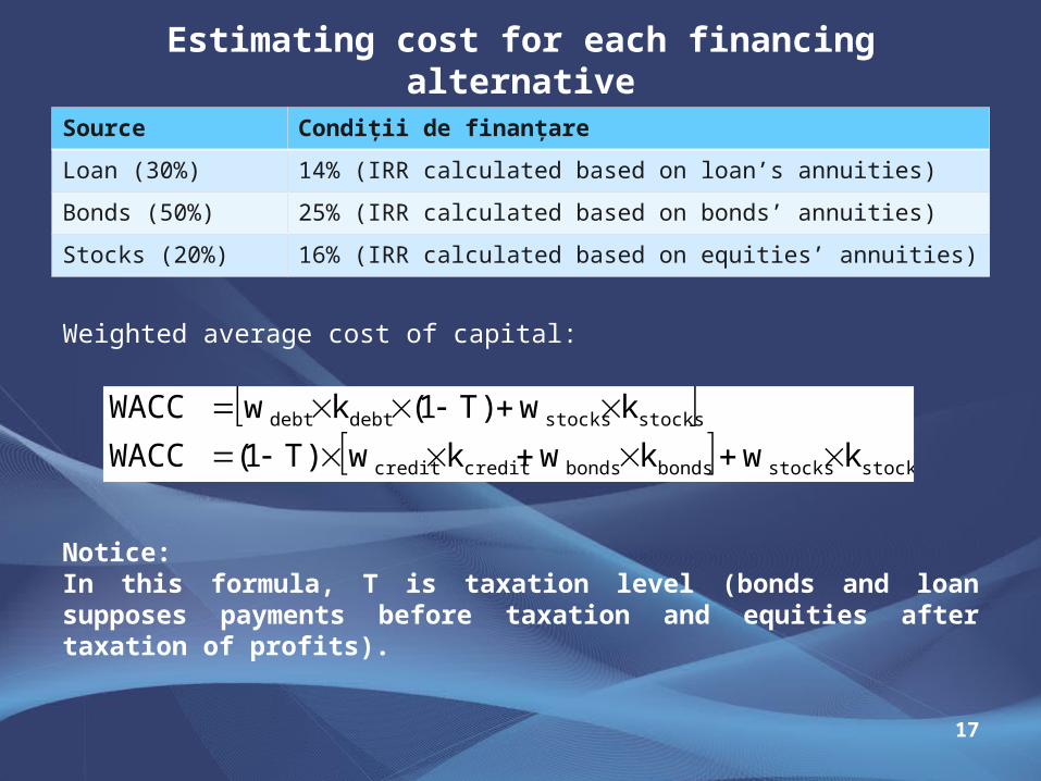
Estimating cost for each financing alternative

17

Source Condiţii de finanţare

Loan (30%) 14% (IRR calculated based on loan’s annuities)

Bonds (50%) 25% (IRR calculated based on bonds’ annuities)

Stocks (20%) 16% (IRR calculated based on equities’ annuities)

Weighted average cost of capital:

Notice:In this formula, T is taxation level (bonds and loan supposes payments before taxation and equities after taxation of profits).

stocksstocksbondsbondscreditcredit

stocksstocksdebtdebt

kwkwkw)T1(WACC

kw)T1(kwWACC

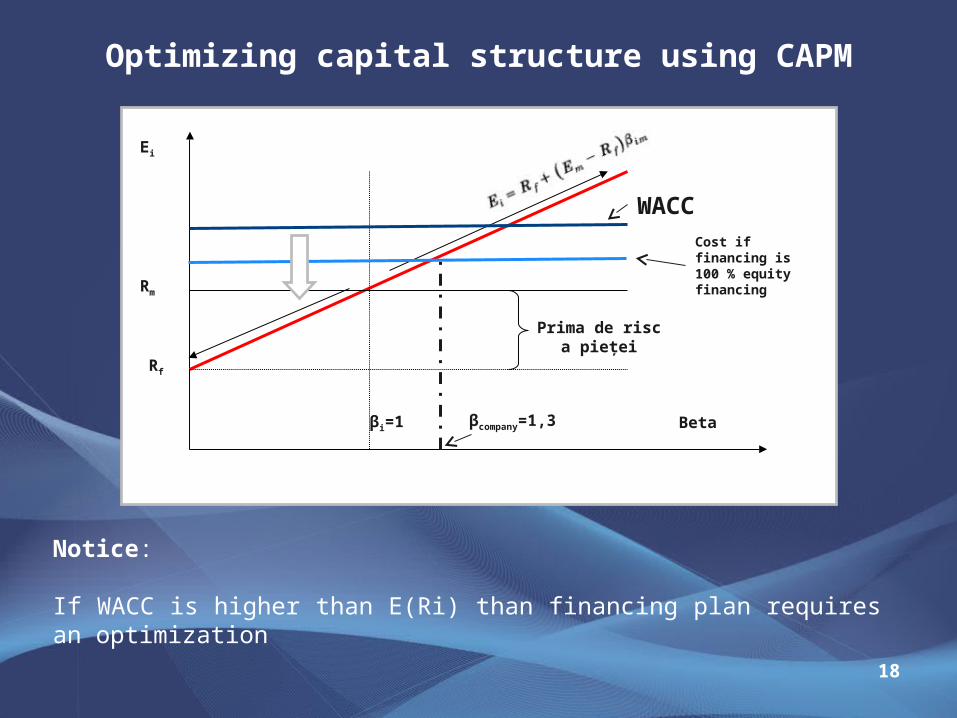
Optimizing capital structure using CAPM

18

Rf

Rm

Ei

Betaβi=1

Prima de risc a pieţei

WACC

βcompany=1,3

Cost if financing is 100 % equity financing

Notice:

If WACC is higher than E(Ri) than financing plan requires an optimization

19

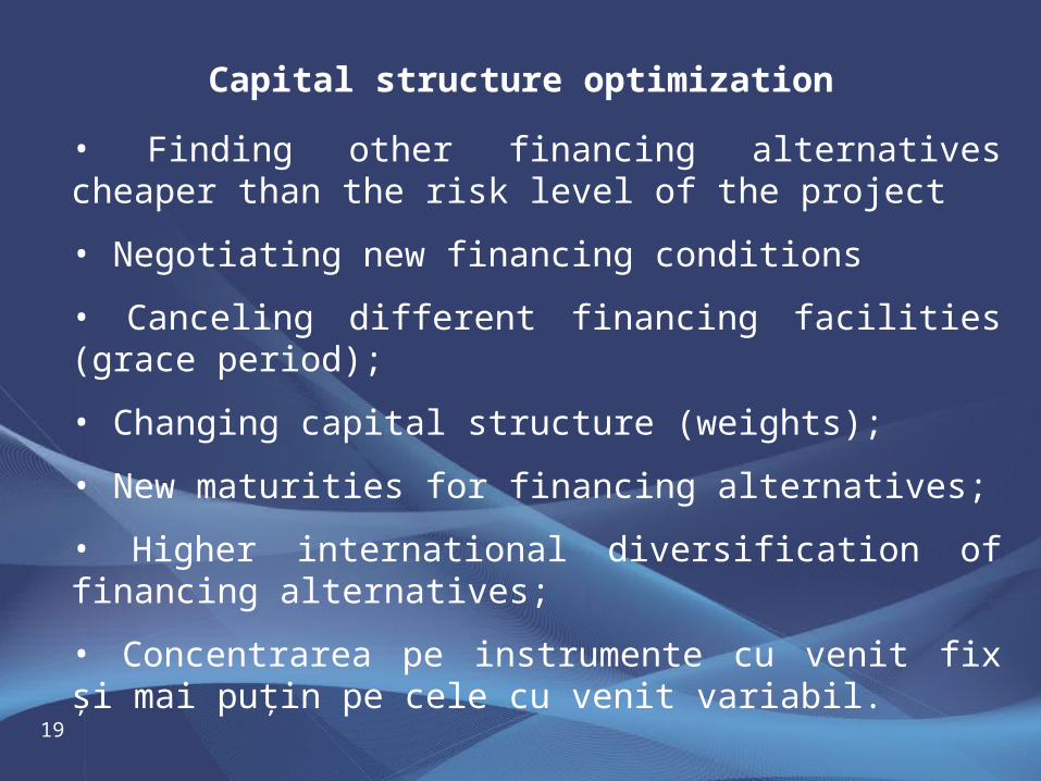
Capital structure optimization

• Finding other financing alternatives cheaper than the risk level of the project

• Negotiating new financing conditions

• Canceling different financing facilities (grace period);

• Changing capital structure (weights);

• New maturities for financing alternatives;

• Higher international diversification of financing alternatives;

• Concentrarea pe instrumente cu venit fix şi mai puţin pe cele cu venit variabil.

Project valuation

www.finint.ase.ro

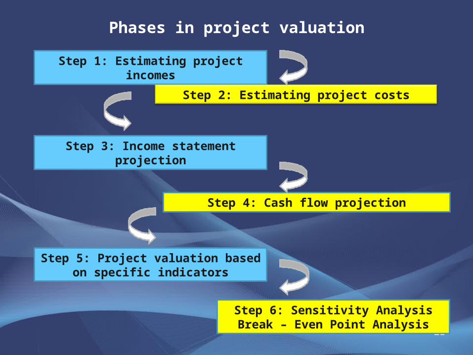
Phases in project valuation

21

Step 1: Estimating project incomes

Step 2: Estimating project costs

Step 3: Income statement projection

Step 4: Cash flow projection

Step 5: Project valuation based on specific indicators

Step 6: Sensitivity AnalysisBreak – Even Point Analysis

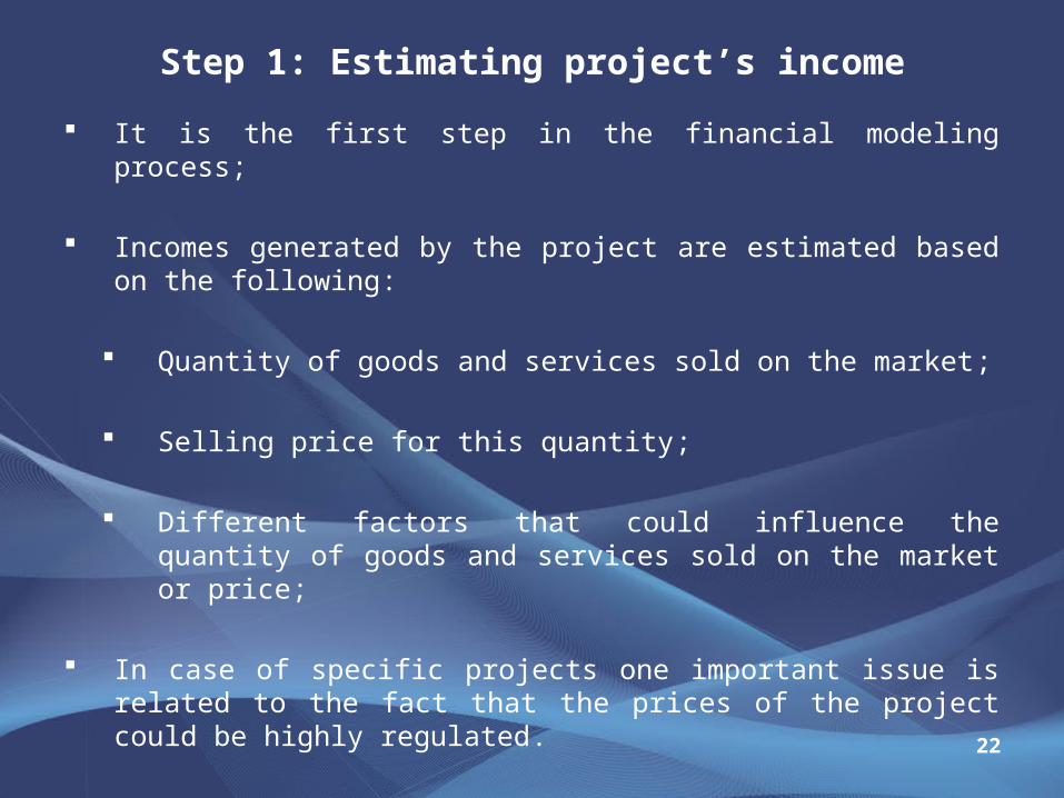
Step 1: Estimating project’s income

22

It is the first step in the financial modeling process;

Incomes generated by the project are estimated based on the following:

Quantity of goods and services sold on the market;

Selling price for this quantity;

Different factors that could influence the quantity of goods and services sold on the market or price;

In case of specific projects one important issue is related to the fact that the prices of the project could be highly regulated.

Step 2: Estimating the project’s costs

23

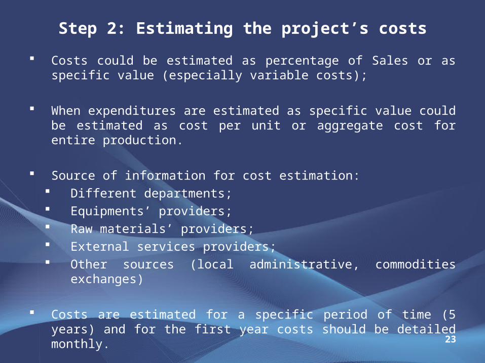
Costs could be estimated as percentage of Sales or as specific value (especially variable costs);

When expenditures are estimated as specific value could be estimated as cost per unit or aggregate cost for entire production.

Source of information for cost estimation: Different departments; Equipments’ providers; Raw materials’ providers; External services providers; Other sources (local administrative, commodities exchanges)

Costs are estimated for a specific period of time (5 years) and for the first year costs should be detailed monthly.

Types of expenditures

24

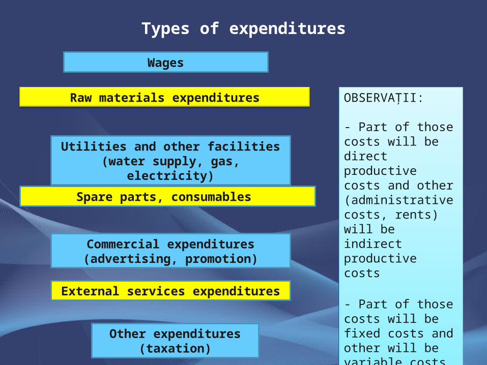
Wages

Raw materials expenditures

Utilities and other facilities (water supply, gas, electricity)

Spare parts, consumables

Commercial expenditures (advertising, promotion)

External services expenditures

Other expenditures (taxation)

OBSERVAŢII:

- Part of those costs will be direct productive costs and other (administrative costs, rents) will be indirect productive costs

- Part of those costs will be fixed costs and other will be variable costs

OBSERVAŢII:

- Part of those costs will be direct productive costs and other (administrative costs, rents) will be indirect productive costs

- Part of those costs will be fixed costs and other will be variable costs

Expenditure projection

25

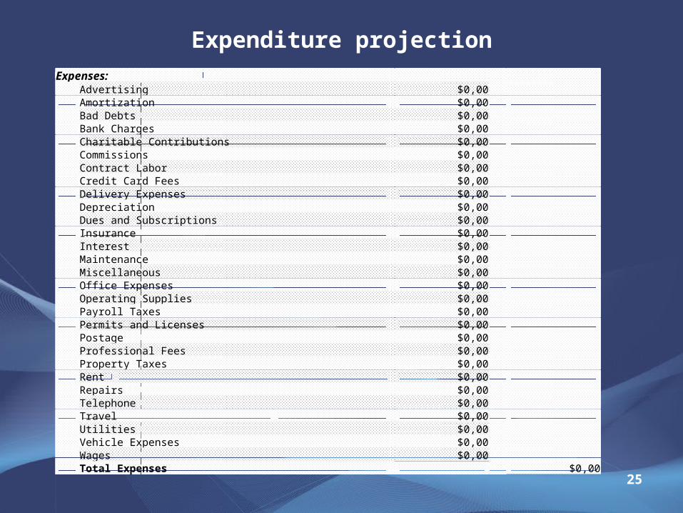
Expenses: Advertising $0,00 Amortization $0,00 Bad Debts $0,00 Bank Charges $0,00 Charitable Contributions $0,00 Commissions $0,00 Contract Labor $0,00 Credit Card Fees $0,00 Delivery Expenses $0,00 Depreciation $0,00 Dues and Subscriptions $0,00 Insurance $0,00 Interest $0,00 Maintenance $0,00 Miscellaneous $0,00 Office Expenses $0,00 Operating Supplies $0,00 Payroll Taxes $0,00 Permits and Licenses $0,00 Postage $0,00 Professional Fees $0,00 Property Taxes $0,00 Rent $0,00 Repairs $0,00 Telephone $0,00 Travel $0,00 Utilities $0,00 Vehicle Expenses $0,00 Wages $0,00 Total Expenses $0,00

Step 3: Income statement and balance sheet projection

26

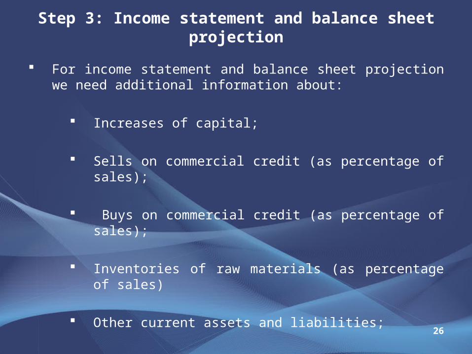
For income statement and balance sheet projection we need additional information about:

Increases of capital;

Sells on commercial credit (as percentage of sales);

Buys on commercial credit (as percentage of sales);

Inventories of raw materials (as percentage of sales)

Other current assets and liabilities;

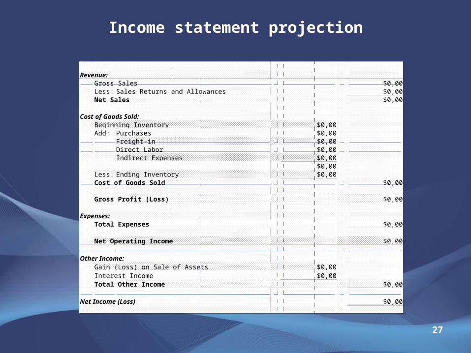
Income statement projection

27

Revenue: Gross Sales $0,00 Less: Sales Returns and Allowances $0,00 Net Sales $0,00 Cost of Goods Sold: Beginning Inventory $0,00 Add: Purchases $0,00 Freight-in $0,00 Direct Labor $0,00 Indirect Expenses $0,00 $0,00 Less: Ending Inventory $0,00 Cost of Goods Sold $0,00 Gross Profit (Loss) $0,00 Expenses: Total Expenses $0,00 Net Operating Income $0,00 Other Income: Gain (Loss) on Sale of Assets $0,00 Interest Income $0,00 Total Other Income $0,00 Net Income (Loss) $0,00

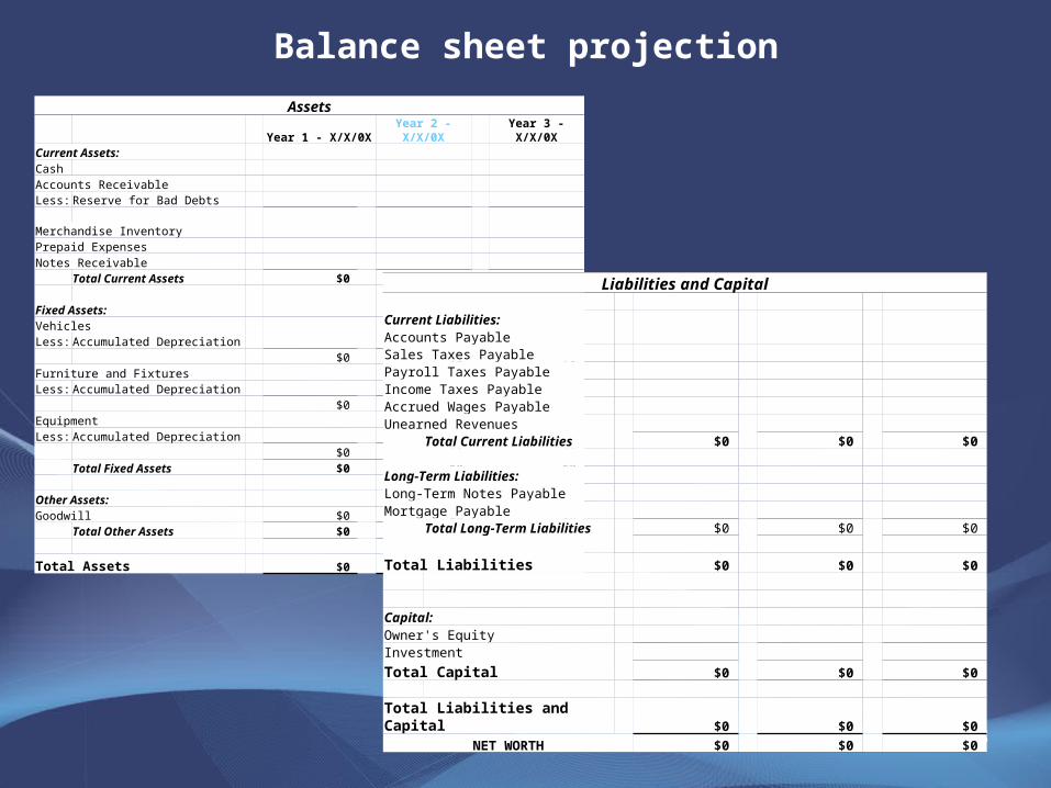
Balance sheet projection

28

AssetsYear 1 - X/X/0X Year 2 - X/X/0X Year 3 - X/X/0X

Current Assets:CashAccounts Receivable Less: Reserve for Bad Debts

Merchandise Inventory Prepaid Expenses Notes Receivable

Total Current Assets $0 $0 $0 Fixed Assets: Vehicles Less: Accumulated Depreciation

$0 $0 $0 Furniture and FixturesLess: Accumulated Depreciation

$0 $0 $0 Equipment Less: Accumulated Depreciation

$0 $0 $0 Total Fixed Assets $0 $0 $0

Other Assets: Goodwill $0 $0 $0

Total Other Assets $0 $0 $0

Total Assets $0 $0 $0

Liabilities and Capital

Current Liabilities:Accounts PayableSales Taxes PayablePayroll Taxes Payable Income Taxes PayableAccrued Wages Payable Unearned Revenues

Total Current Liabilities $0 $0 $0

Long-Term Liabilities: Long-Term Notes PayableMortgage Payable

Total Long-Term Liabilities $0 $0 $0

Total Liabilities $0 $0 $0

Capital: Owner's Equity Investment

Total Capital $0 $0 $0

Total Liabilities and Capital $0 $0 $0

NET WORTH $0 $0 $0

Step 4: Cash flow projection

29

Cash flow is different than net profit because it reconsiders the value of fixed assets depreciation;

It is calculated as difference between inflows (incomes from sales for instance) and outflows (expenditures) of the project;

There are three different components of project’s cash flow:

Operating cash flow;

Investment cash flow;

Financing cash flow.

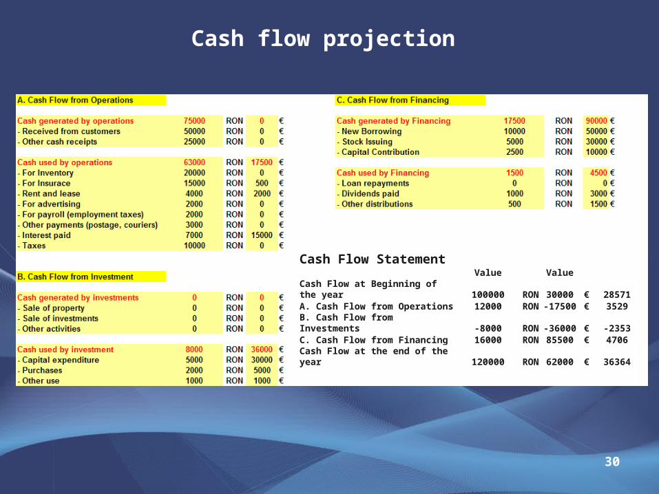
Cash flow projection

30

Cash Flow StatementValue Value

Cash Flow at Beginning of the year 100000 RON 30000 € 28571A. Cash Flow from Operations 12000 RON -17500 € 3529B. Cash Flow from Investments -8000 RON -36000 € -2353C. Cash Flow from Financing 16000 RON 85500 € 4706Cash Flow at the end of the year 120000 RON 62000 € 36364

Step 5: Investment project valuation

31

The indicators used to evaluate the project are the following:

Net present value (NPV);

Internal Rate of Return (IRR);

Recovery Period of Investment (RPI);

Profitability Index (PI).

NPV Criterion in Project Valuation

32

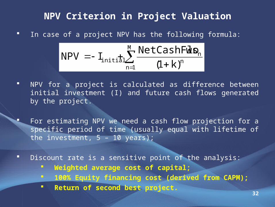
In case of a project NPV has the following formula:

NPV for a project is calculated as difference between initial investment (I) and future cash flows generated by the project.

For estimating NPV we need a cash flow projection for a specific period of time (usually equal with lifetime of the investment, 5 – 10 years);

Discount rate is a sensitive point of the analysis: Weighted average cost of capital; 100% Equity financing cost (derived from CAPM); Return of second best project.

M

1nn

ninitial )k1(

wsNetCashFloINPV

IRR criterion in investment project

33

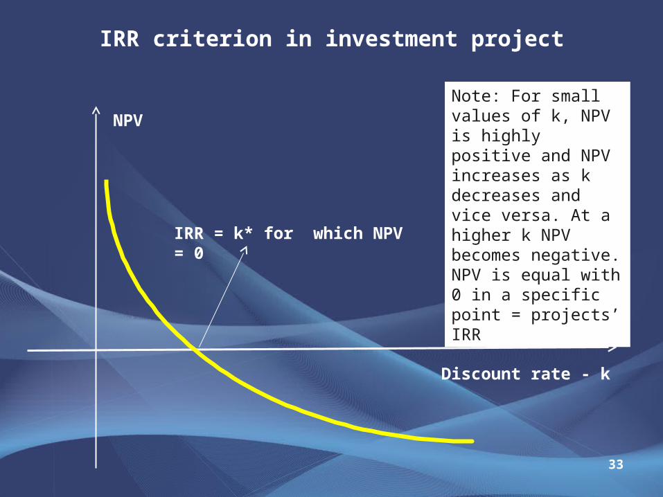
Note: For small values of k, NPV is highly positive and NPV increases as k decreases and vice versa. At a higher k NPV becomes negative.NPV is equal with 0 in a specific point = projects’ IRR

IRR = k* for which NPV = 0

NPV

Discount rate - k

Modified IRR (MIRR)

34

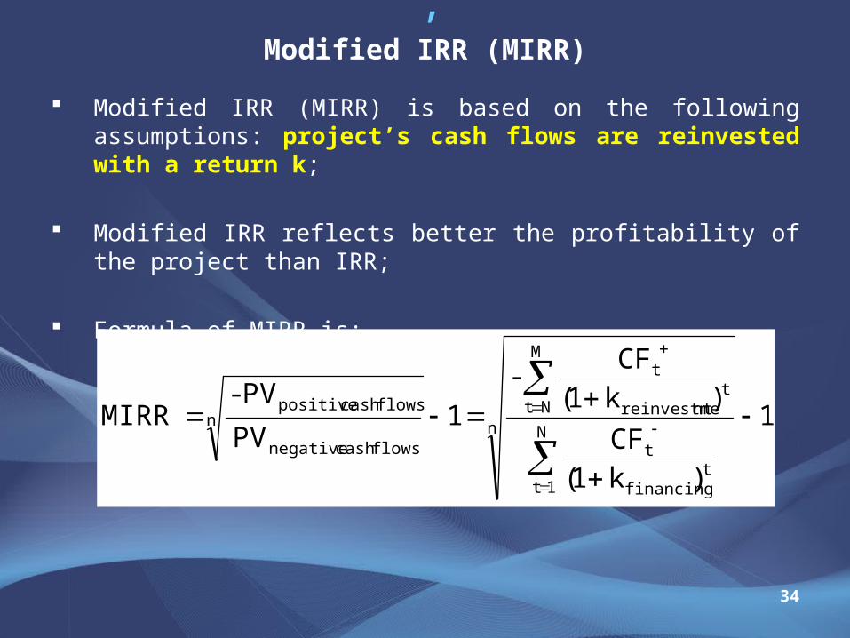
Modified IRR (MIRR) is based on the following assumptions: project’s cash flows are reinvested with a return k;

Modified IRR reflects better the profitability of the project than IRR;

Formula of MIRR is:

,

1

)k1(

)k1(1

N

1tt

financing

M

Ntt

ntreinvestme

nt

t

n

flowscash negative

flowscash positive

CF

CF-

PV

PV-MIRR

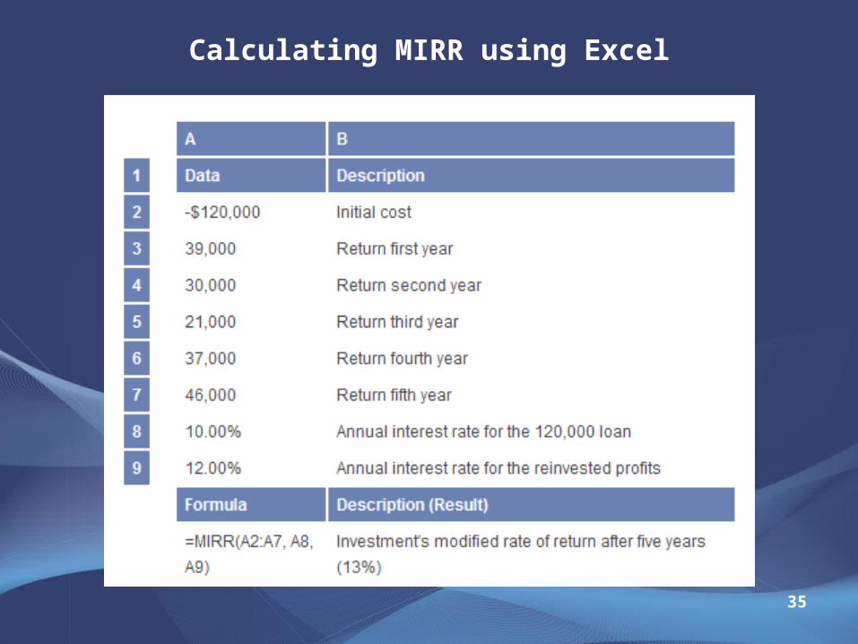
Calculating MIRR using Excel

35

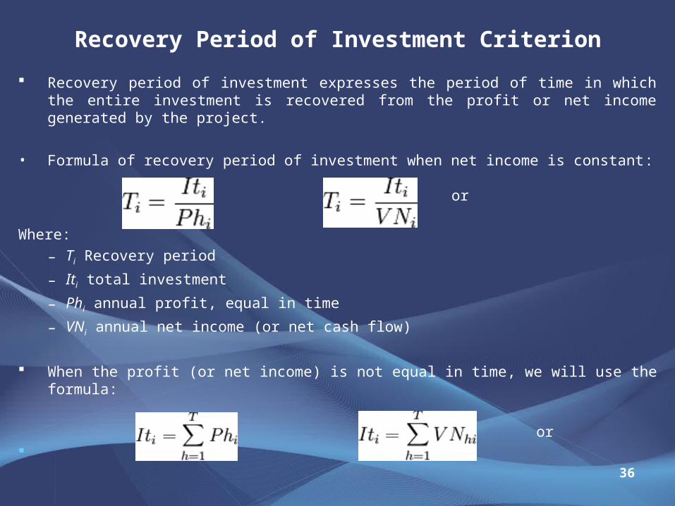
Recovery Period of Investment Criterion

36

Recovery period of investment expresses the period of time in which the entire investment is recovered from the profit or net income generated by the project.

• Formula of recovery period of investment when net income is constant:

or

Where:

– Ti Recovery period

– Iti total investment

– Phi annual profit, equal in time

– VNi annual net income (or net cash flow)

When the profit (or net income) is not equal in time, we will use the formula:

or

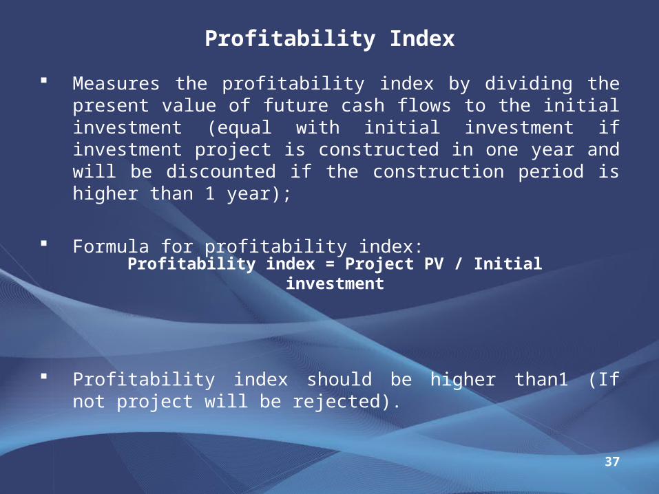
Profitability Index

37

Measures the profitability index by dividing the present value of future cash flows to the initial investment (equal with initial investment if investment project is constructed in one year and will be discounted if the construction period is higher than 1 year);

Formula for profitability index:

Profitability index should be higher than1 (If not project will be rejected).

Profitability index = Project PV / Initial investment

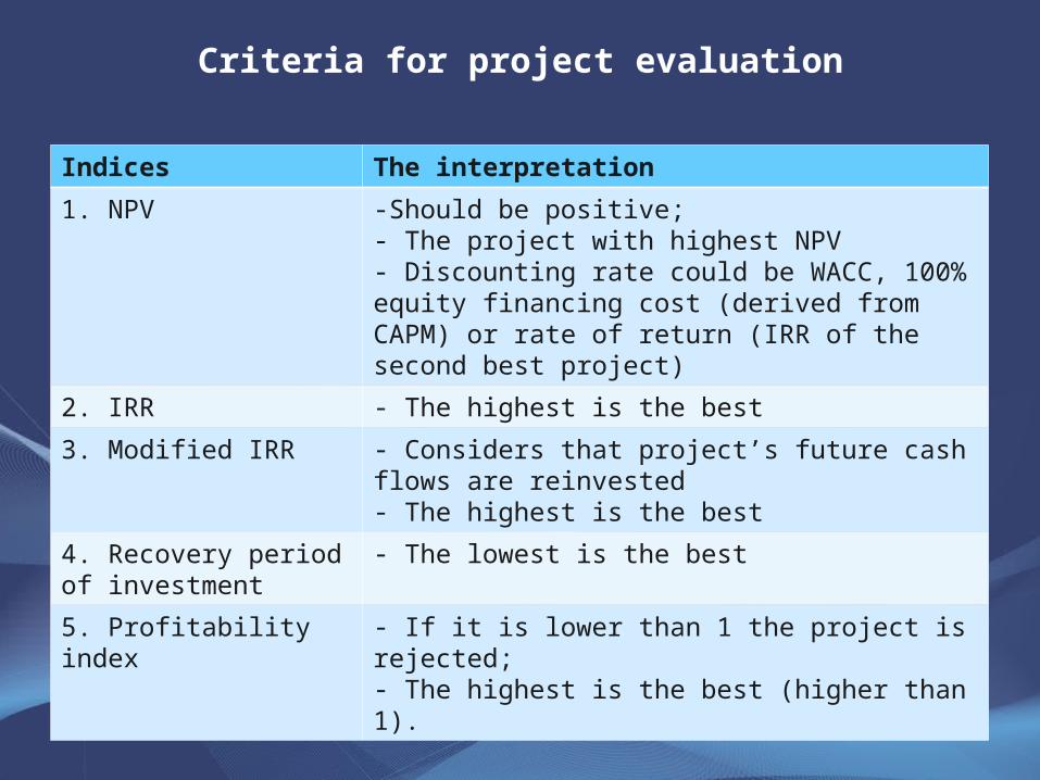
Criteria for project evaluation

38

Indices The interpretation

1. NPV -Should be positive;- The project with highest NPV- Discounting rate could be WACC, 100% equity financing cost (derived from CAPM) or rate of return (IRR of the second best project)

2. IRR - The highest is the best

3. Modified IRR - Considers that project’s future cash flows are reinvested- The highest is the best

4. Recovery period of investment

- The lowest is the best

5. Profitability index - If it is lower than 1 the project is rejected;- The highest is the best (higher than 1).

Sensitivity Analysis

39

Supposes a change in different variables of the project that will change the parameters of the project;

Before running such analysis we should identify the most important risk factors for the project:

Sales volume;

Other variable expenditures (wages, raw materials, external services, materials);

Financing expenditures (interest rate).


40

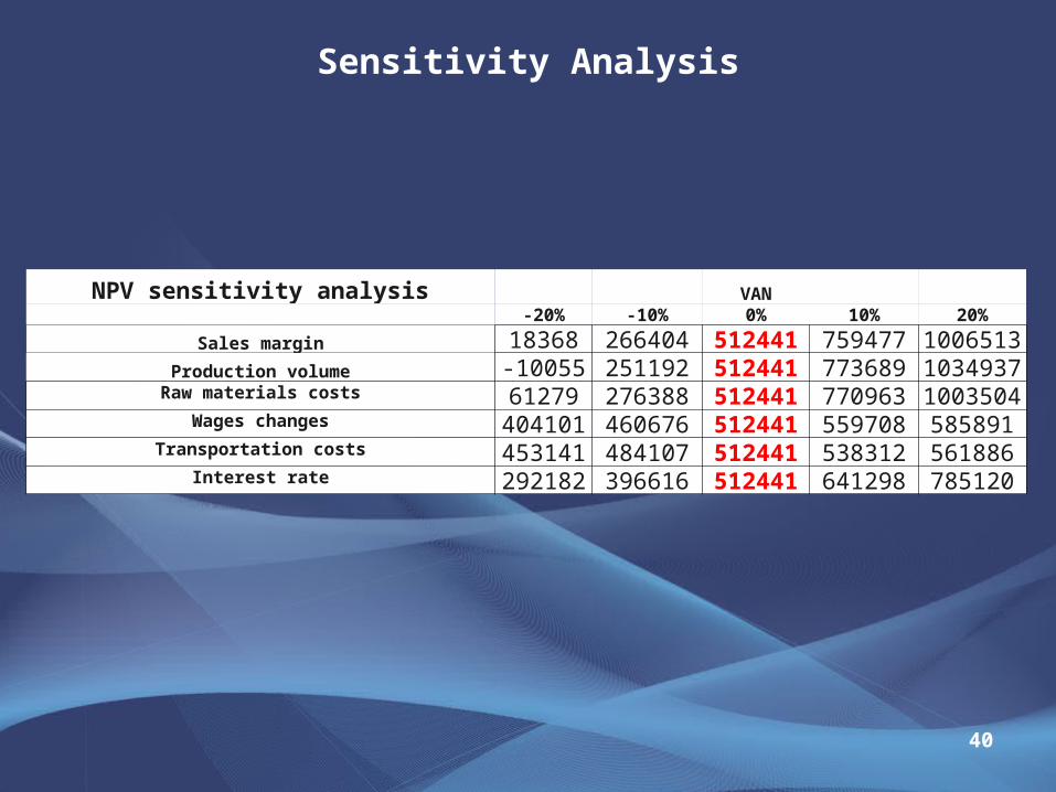
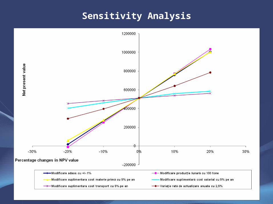
NPV sensitivity analysis VAN-20% -10% 0% 10% 20%

Sales margin 18368 266404 512441 759477 1006513Production volume -10055 251192 512441 773689 1034937Raw materials costs 61279 276388 512441 770963 1003504

Wages changes 404101 460676 512441 559708 585891Transportation costs 453141 484107 512441 538312 561886

Interest rate 292182 396616 512441 641298 785120


41

Break – Even Point Analysis

42

Determines the point from where the project starts to be a profitable one (break – even point);

This analysis completes the sensitivity analysis offering a different perspective on the minimum value of sales from where the project becomes profitable.

The most used break-even methods are:

1. ACCOUNTING BREAK-EVEN ANALYSIS

2. NPV BREAK-EVEN ANALYSIS

ACCOUNTING BREAK – EVEN ANALYSIS

43

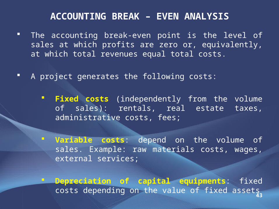
The accounting break-even point is the level of sales at which profits are zero or, equivalently, at which total revenues equal total costs.

A project generates the following costs:

Fixed costs (independently from the volume of sales): rentals, real estate taxes, administrative costs, fees;

Variable costs: depend on the volume of sales. Example: raw materials costs, wages, external services;

Depreciation of capital equipments: fixed costs depending on the value of fixed assets

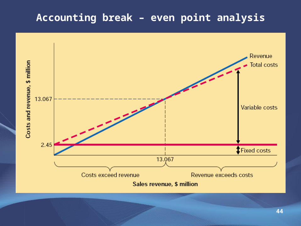
Accounting break – even point analysis

44

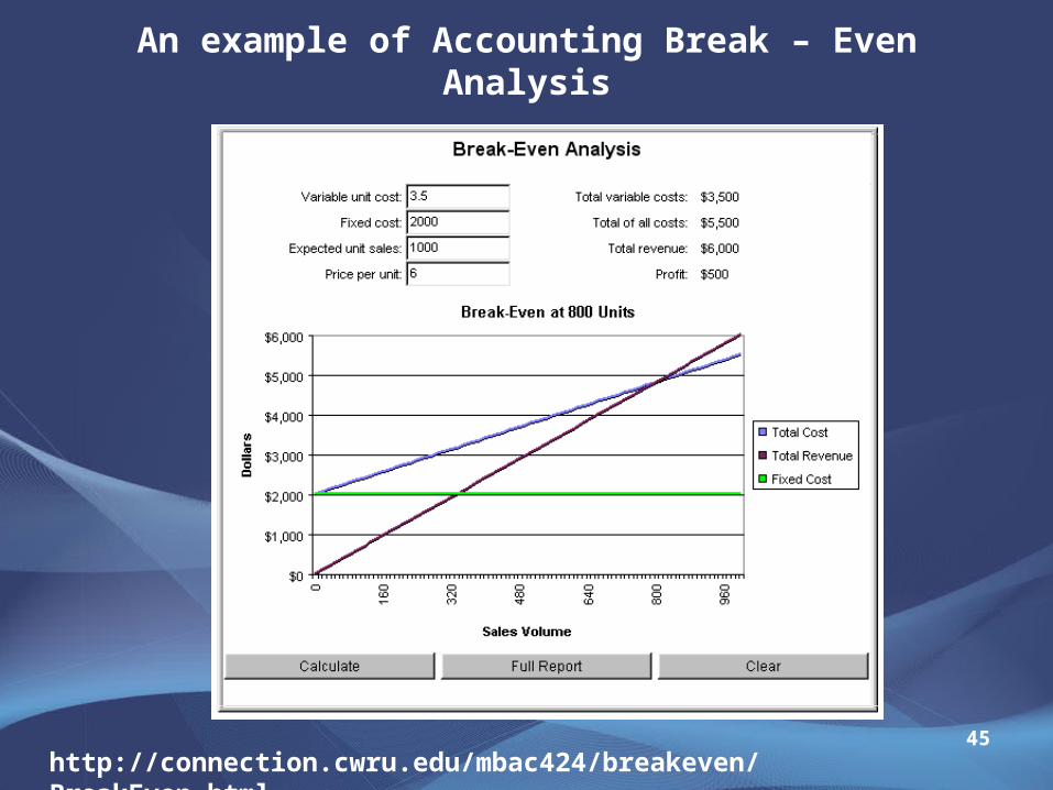
An example of Accounting Break – Even Analysis

45http://connection.cwru.edu/mbac424/breakeven/BreakEven.html

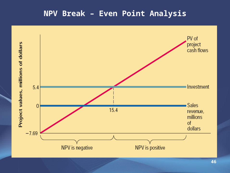
NPV Break – Even Point Analysis

46

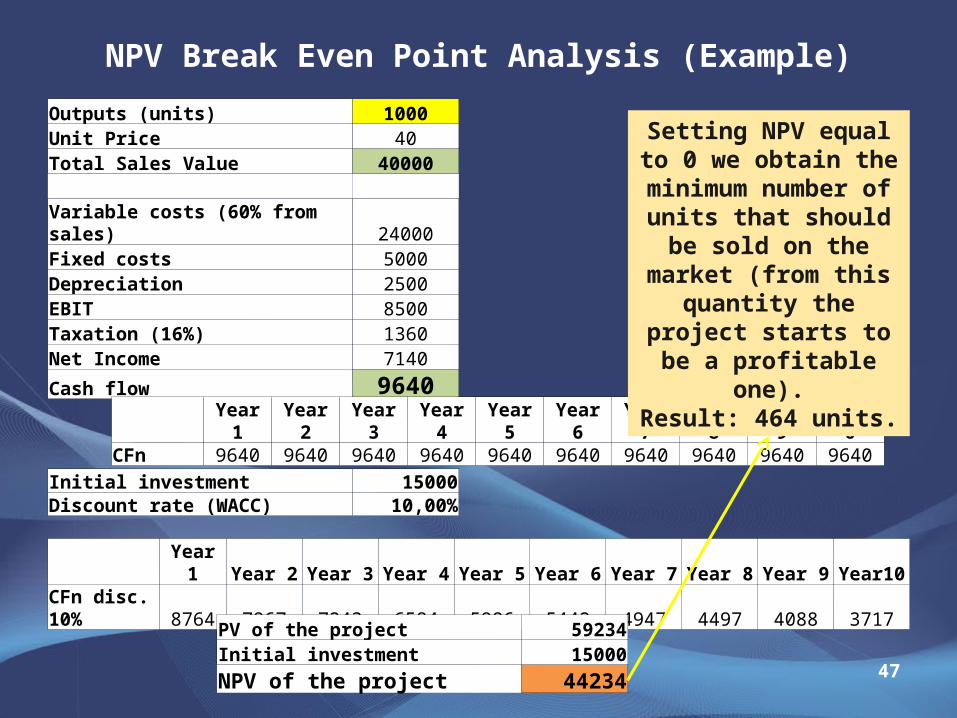
NPV Break Even Point Analysis (Example)

47

Outputs (units) 1000Unit Price 40Total Sales Value 40000 Variable costs (60% from sales) 24000Fixed costs 5000Depreciation 2500EBIT 8500Taxation (16%) 1360Net Income 7140

Cash flow 9640

Year 1 Year 2 Year 3 Year 4 Year 5 Year 6 Year 7 Year 8 Year 9 Year10CFn 9640 9640 9640 9640 9640 9640 9640 9640 9640 9640

Initial investment 15000Discount rate (WACC) 10,00%

Year 1 Year 2 Year 3 Year 4 Year 5 Year 6 Year 7 Year 8 Year 9 Year10CFn disc. 10% 8764 7967 7243 6584 5986 5442 4947 4497 4088 3717

PV of the project 59234Initial investment 15000NPV of the project 44234

Setting NPV equal to 0 we obtain the

minimum number of units that should be sold on the market

(from this quantity the project starts to be a

profitable one).Result: 464 units.

Operating Leverage Analysis

48

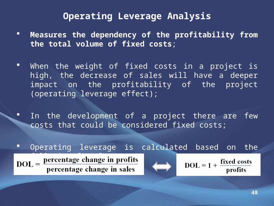
Measures the dependency of the profitability from the total volume of fixed costs;

When the weight of fixed costs in a project is high, the decrease of sales will have a deeper impact on the profitability of the project (operating leverage effect);

In the development of a project there are few costs that could be considered fixed costs;

Operating leverage is calculated based on the following formula:

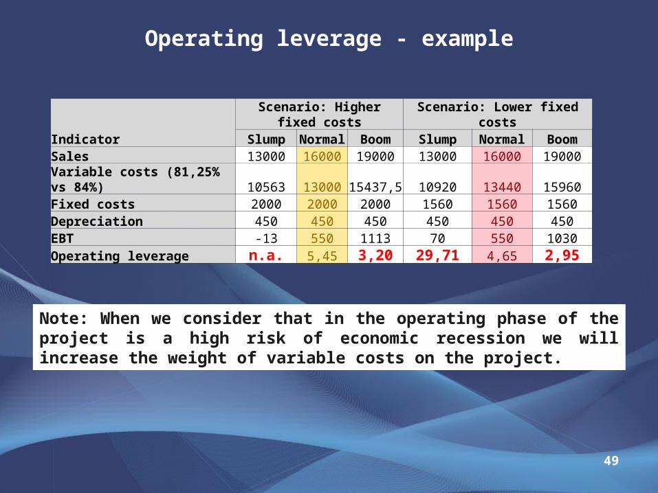
Operating leverage - example

49

IndicatorScenario: Higher fixed costs Scenario: Lower fixed costsSlump Normal Boom Slump Normal Boom

Sales 13000 16000 19000 13000 16000 19000Variable costs (81,25% vs 84%) 10563 13000 15437,5 10920 13440 15960Fixed costs 2000 2000 2000 1560 1560 1560Depreciation 450 450 450 450 450 450EBT -13 550 1113 70 550 1030Operating leverage n.a. 5,45 3,20 29,71 4,65 2,95

Note: When we consider that in the operating phase of the project is a high risk of economic recession we will increase the weight of variable costs on the project.

Documents

Lecture 8: Cost of capital. Financial modeling of a project