1

Steel, Lecture 3

Column buckling Only axial loading

Axial and transverse loading

by

Bert Norlin

2

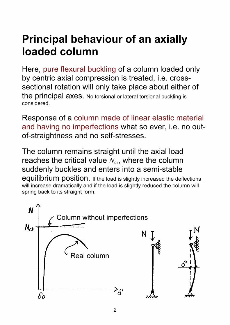
Principal behaviour of an axially loaded column Here, pure flexural buckling of a column loaded only by centric axial compression is treated, i.e. cross-sectional rotation will only take place about either of the principal axes. No torsional or lateral torsional buckling is considered.

Response of a column made of linear elastic material and having no imperfections what so ever, i.e. no out-of-straightness and no self-stresses.

The column remains straight until the axial load reaches the critical value Ncr, where the column suddenly buckles and enters into a semi-stable equilibrium position. If the load is slightly increased the deflections will increase dramatically and if the load is slightly reduced the column will spring back to its straight form.

Column without imperfections

Real column

3

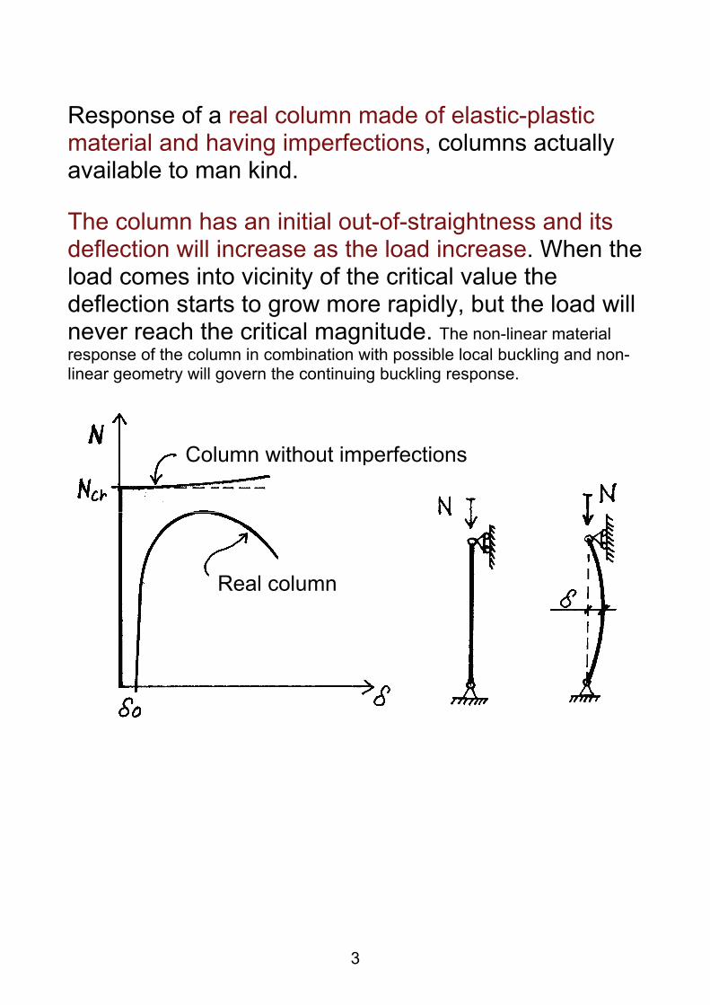
Response of a real column made of elastic-plastic material and having imperfections, columns actually available to man kind.

The column has an initial out-of-straightness and its deflection will increase as the load increase. When the load comes into vicinity of the critical value the deflection starts to grow more rapidly, but the load will never reach the critical magnitude. The non-linear material response of the column in combination with possible local buckling and non-linear geometry will govern the continuing buckling response.

Column without imperfections

Real column

4

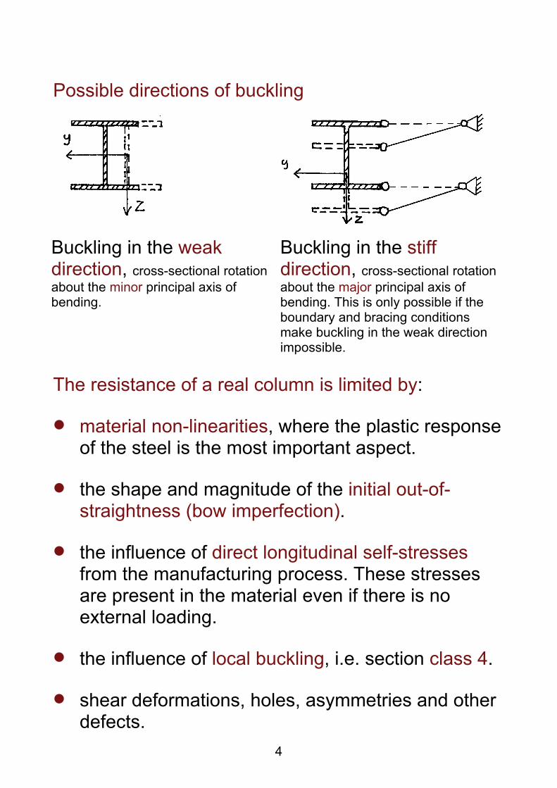
Possible directions of buckling

Buckling in the weak direction, cross-sectional rotation about the minor principal axis of bending.

Buckling in the stiff direction, cross-sectional rotation about the major principal axis of bending. This is only possible if the boundary and bracing conditions make buckling in the weak direction impossible.

The resistance of a real column is limited by:

• material non-linearities, where the plastic response of the steel is the most important aspect.

• the shape and magnitude of the initial out-of-straightness (bow imperfection).

• the influence of direct longitudinal self-stresses from the manufacturing process. These stresses are present in the material even if there is no external loading.

• the influence of local buckling, i.e. section class 4.

• shear deformations, holes, asymmetries and other defects.

5

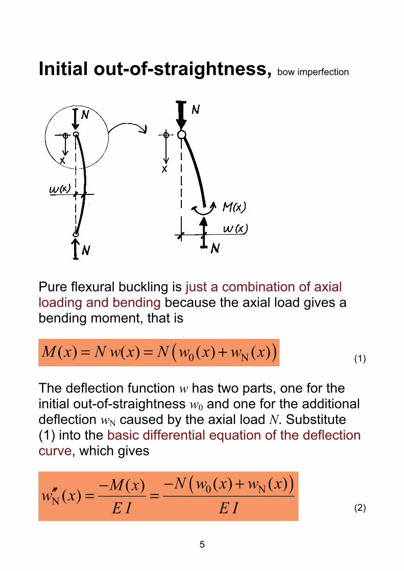
Initial out-of-straightness, bow imperfection

Pure flexural buckling is just a combination of axial loading and bending because the axial load gives a bending moment, that is

( )0 N( ) ( ) ( ) ( )M x N w x N w x w x= = + (1)

The deflection function w has two parts, one for the initial out-of-straightness w0 and one for the additional deflection wN caused by the axial load N. Substitute (1) into the basic differential equation of the deflection curve, which gives

( )0 NN

( ) ( )( )( )N w x w xM xw x

E I E I− +−′′ = =

(2)

6

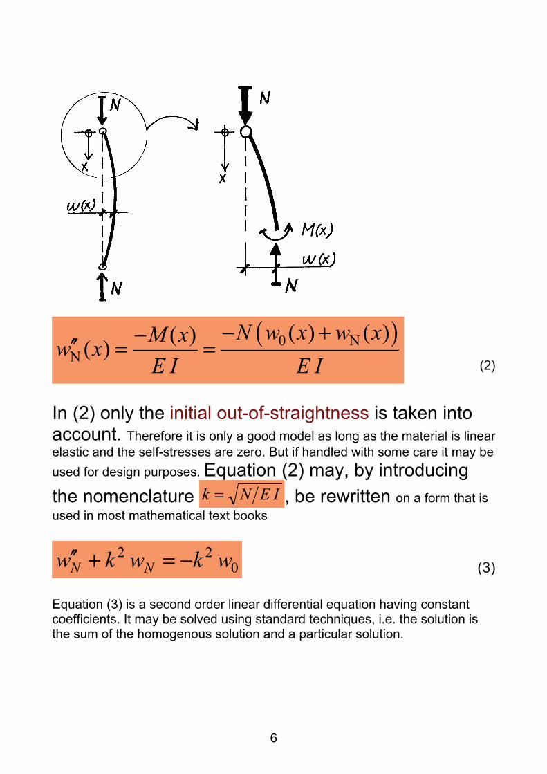
( )0 NN

( ) ( )( )( )N w x w xM xw x

E I E I− +−′′ = =

(2)

In (2) only the initial out-of-straightness is taken into account. Therefore it is only a good model as long as the material is linear elastic and the self-stresses are zero. But if handled with some care it may be used for design purposes. Equation (2) may, by introducing the nomenclature IENk = , be rewritten on a form that is used in most mathematical text books

022 wkwkw NN −=+′′ (3)

Equation (3) is a second order linear differential equation having constant coefficients. It may be solved using standard techniques, i.e. the solution is the sum of the homogenous solution and a particular solution.

7

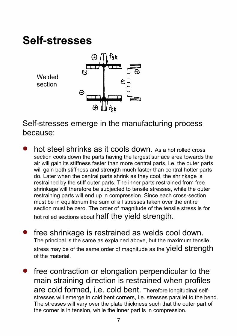
Self-stresses

Self-stresses emerge in the manufacturing process because:

• hot steel shrinks as it cools down. As a hot rolled cross section cools down the parts having the largest surface area towards the air will gain its stiffness faster than more central parts, i.e. the outer parts will gain both stiffness and strength much faster than central hotter parts do. Later when the central parts shrink as they cool, the shrinkage is restrained by the stiff outer parts. The inner parts restrained from free shrinkage will therefore be subjected to tensile stresses, while the outer restraining parts will end up in compression. Since each cross-section must be in equilibrium the sum of all stresses taken over the entire section must be zero. The order of magnitude of the tensile stress is for hot rolled sections about half the yield strength.

• free shrinkage is restrained as welds cool down. The principal is the same as explained above, but the maximum tensile stress may be of the same order of magnitude as the yield strength of the material.

• free contraction or elongation perpendicular to the main straining direction is restrained when profiles are cold formed, i.e. cold bent. Therefore longitudinal self-stresses will emerge in cold bent corners, i.e. stresses parallel to the bend. The stresses will vary over the plate thickness such that the outer part of the corner is in tension, while the inner part is in compression.

Welded section

8

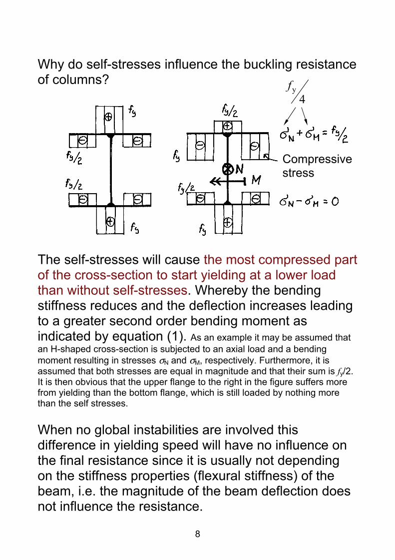
Why do self-stresses influence the buckling resistance of columns?

The self-stresses will cause the most compressed part of the cross-section to start yielding at a lower load than without self-stresses. Whereby the bending stiffness reduces and the deflection increases leading to a greater second order bending moment as indicated by equation (1). As an example it may be assumed that an H-shaped cross-section is subjected to an axial load and a bending moment resulting in stresses σN and σM, respectively. Furthermore, it is assumed that both stresses are equal in magnitude and that their sum is fy/2. It is then obvious that the upper flange to the right in the figure suffers more from yielding than the bottom flange, which is still loaded by nothing more than the self stresses.

When no global instabilities are involved this difference in yielding speed will have no influence on the final resistance since it is usually not depending on the stiffness properties (flexural stiffness) of the beam, i.e. the magnitude of the beam deflection does not influence the resistance.

Compressive stress

4yf

9

Resistance with regard to flexural buckling for centric axial loading according to EC3 The influence of column buckling is accounted for through the use of a correction factor χ and not through an explicit study of all factors actually influencing the stability. For sections in class 1, 2 or 3 the buckling resistance is

1M

yRdb, γ

χ fAN =

(4), (6.47)

A gross cross-sectional area

γM1 partial coefficient for global instability, usually 1,0

For sections in class 4 the flexural buckling resistance is

1M

yeffRdb, γ

χ fAN =

(5), (6.48)

Aeff effective cross-sectional area due to the influence of local buckling

To calculate the reduction factor χ one has first to determine a slenderness parameter that for section classes 1, 2 and 3 is defined as

10

cr

y

cr

y

NfAf

==σ

λ (6), (6.49)

A fy axial resistance NRk of the gross cross-section when column buckling is not taken into account.

Ncr critical buckling load for a column without imperfections, i.e. the well known Euler buckling load calculated using the gross cross-section.

For sections in class 4 the slenderness is defined as

cr

yeff

NfA

=λ (7), (6.49)

Aeff fy axial resistance Nc,Rk of the effective cross-section when column buckling is not taken into account but local buckling is.

Ncr critical buckling load for a column without imperfections, calculated using the gross cross-section. Note that the critical load is determined using the gross cross-section, which is natural because it depends mostly on the flexural stiffness along the entire beam and not just on the stiffness in the collapsing cross-section.

The reduction factor χ can be read from a buckling diagram when the slenderness parameter λ is known.

11

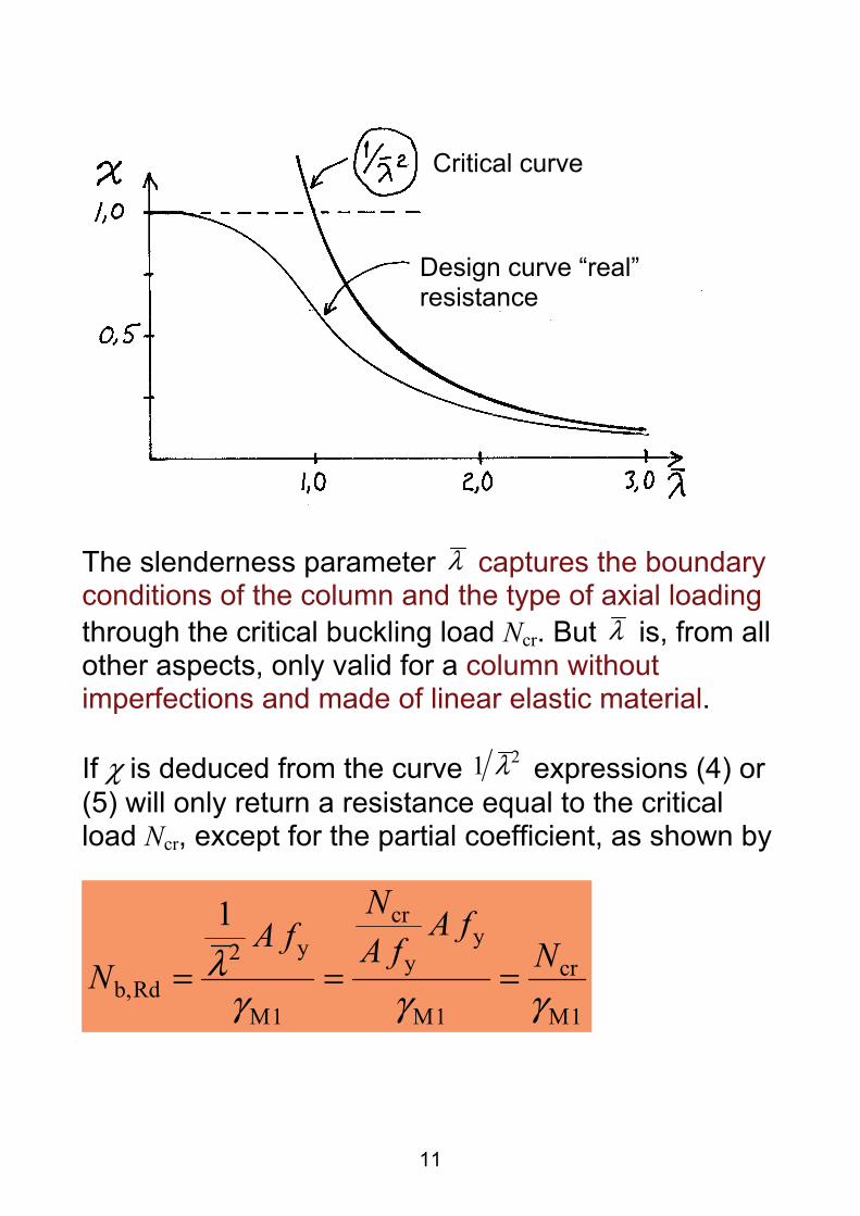
The slenderness parameter λ captures the boundary conditions of the column and the type of axial loading through the critical buckling load Ncr. But λ is, from all other aspects, only valid for a column without imperfections and made of linear elastic material.

If χ is deduced from the curve 21 λ expressions (4) or (5) will only return a resistance equal to the critical load Ncr, except for the partial coefficient, as shown by

1M

cr

1M

yy

cr

1M

y2Rdb,

1

γγγλ N

fAfA

NfA

N ===

Critical curve

Design curve “real” resistance

12

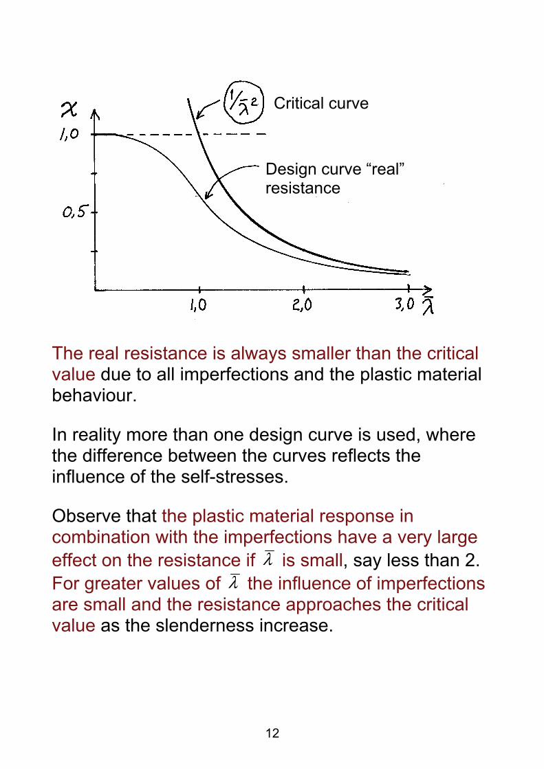
The real resistance is always smaller than the critical value due to all imperfections and the plastic material behaviour.

In reality more than one design curve is used, where the difference between the curves reflects the influence of the self-stresses.

Observe that the plastic material response in combination with the imperfections have a very large effect on the resistance if λ is small, say less than 2. For greater values of λ the influence of imperfections are small and the resistance approaches the critical value as the slenderness increase.

Critical curve

Design curve “real” resistance

13

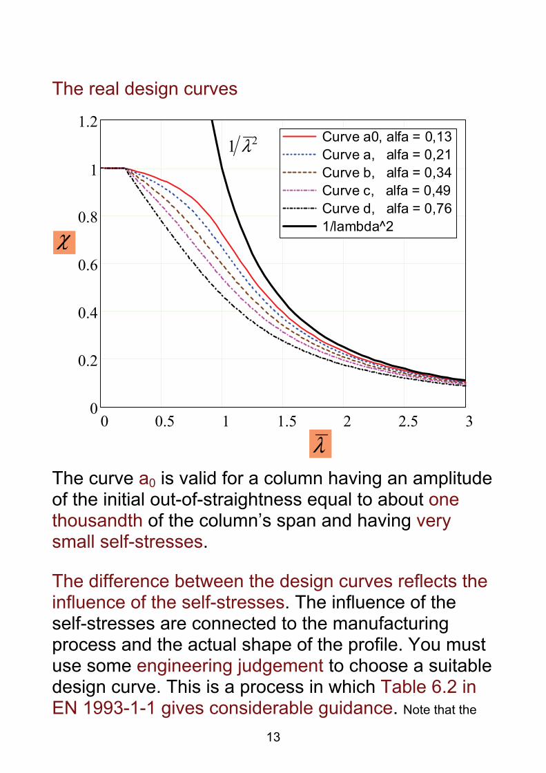
The real design curves

0 0.5 1 1.5 2 2.5 30

0.2

0.4

0.6

0.8

1

1.2Curve a0, alfa = 0,13Curve a, alfa = 0,21Curve b, alfa = 0,34Curve c, alfa = 0,49Curve d, alfa = 0,761/lambda^2

The curve a0 is valid for a column having an amplitude of the initial out-of-straightness equal to about one thousandth of the column’s span and having very small self-stresses.

The difference between the design curves reflects the influence of the self-stresses. The influence of the self-stresses are connected to the manufacturing process and the actual shape of the profile. You must use some engineering judgement to choose a suitable design curve. This is a process in which Table 6.2 in EN 1993-1-1 gives considerable guidance. Note that the

λ

χ

21 λ

14

Table 6.2 does not cover all possible cross-sections and manufacturing processes. If it is not obvious what curve to use one must try to imagine the distribution of self-stresses over the cross-section and then try to figure out how this distribution will affect the resistance. Choose a conservative curve if the influence seems to be large and a less conservative curve if the influence seems small.

The reduction factor χ may be computed using the function expressions of the design curves. These expressions are

2 2

1χλ

=Φ + Φ − (8), (6.49)

where the help parameter Φ is

[ ]2)2,0(15,0 λλα +−+=Φ (9), (6.49)

The difference between the curves is accomplished by the imperfection parameter α, whose value is given by Table 6.1 in EN 1993-1-1.

The influence of column buckling may be totally neglected if

2,0≤λ or 04,0

cr

Ed ≤NN

15

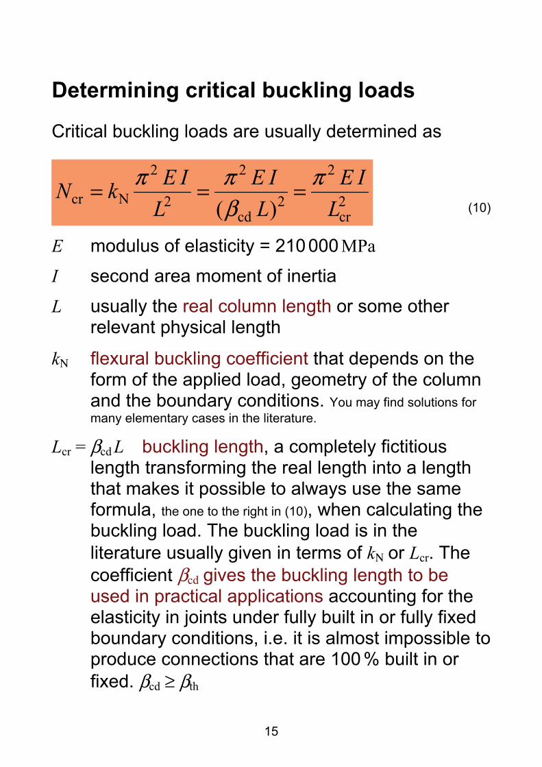
Determining critical buckling loads

Critical buckling loads are usually determined as

2cr

2

2cd

2

2

2

Ncr )( LIE

LIE

LIEkN π

βππ ===

(10)

E modulus of elasticity = 210 000 MPa I second area moment of inertia L usually the real column length or some other

relevant physical length

kΝ flexural buckling coefficient that depends on the form of the applied load, geometry of the column and the boundary conditions. You may find solutions for many elementary cases in the literature.

Lcr = βcd L buckling length, a completely fictitious length transforming the real length into a length that makes it possible to always use the same formula, the one to the right in (10), when calculating the buckling load. The buckling load is in the literature usually given in terms of kΝ or Lcr. The coefficient βcd gives the buckling length to be used in practical applications accounting for the elasticity in joints under fully built in or fully fixed boundary conditions, i.e. it is almost impossible to produce connections that are 100 % built in or fixed. βcd ≥ βth

16

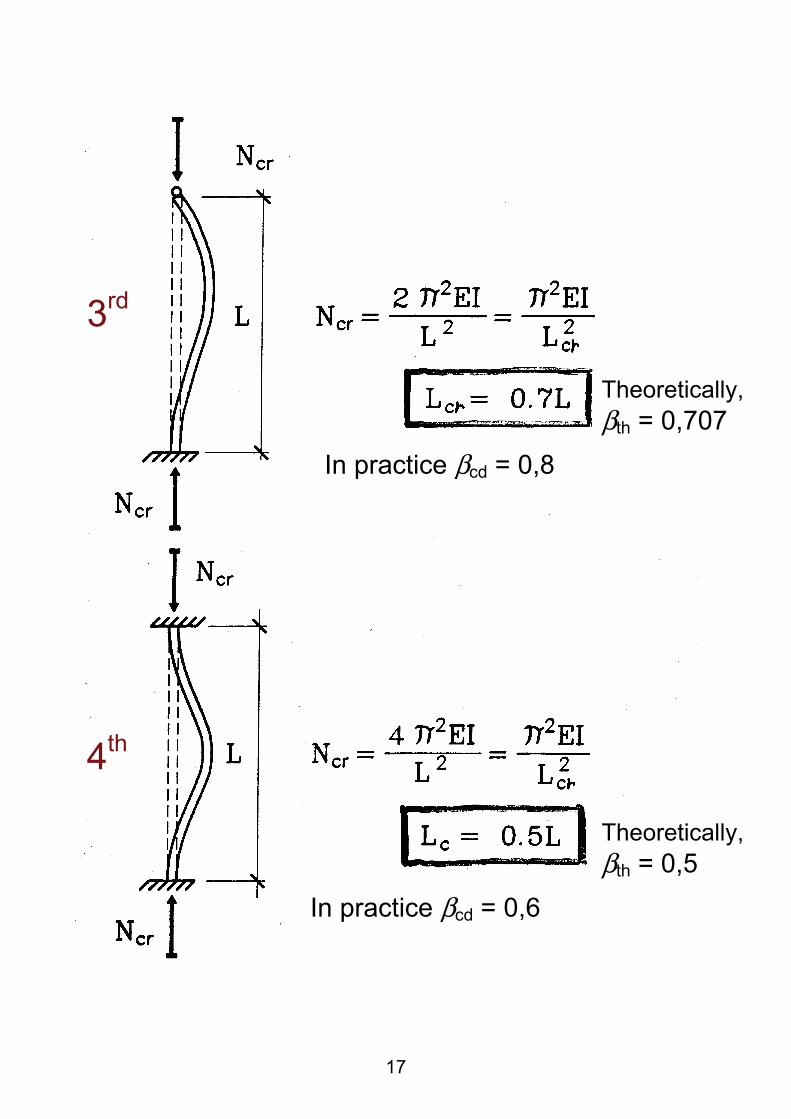
Examples of critical buckling loads, the Euler cases

Theoretically, βth = 2

Theoretically, βth = 2

In practice βcd = 2,1

In practice βcd = 1,0

1st

2nd

17

Theoretically, βth = 0,5

Theoretically, βth = 0,707

In practice βcd = 0,8

In practice βcd = 0,6

3rd

4th

18

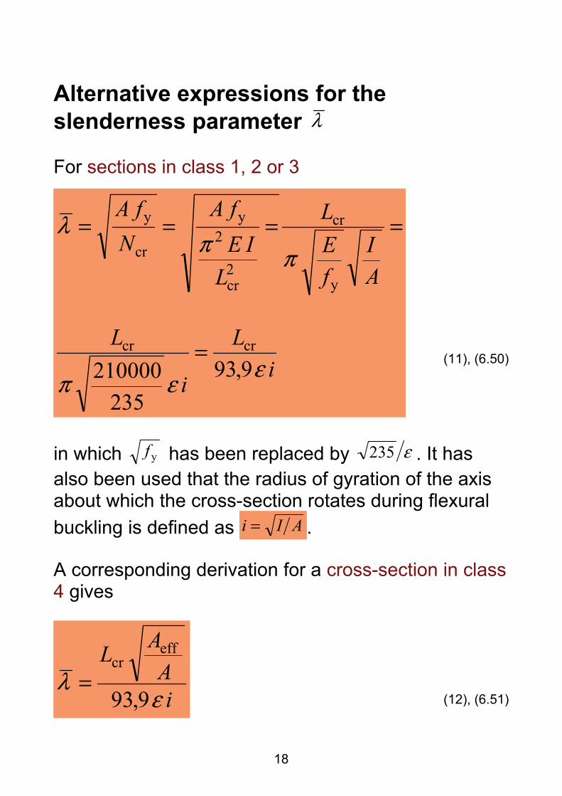
Alternative expressions for the slenderness parameter λ For sections in class 1, 2 or 3

iL

i

L

AI

fEL

LIE

fAN

fA

εεπ

ππλ

9,93235

210000crcr

y

cr

2cr

2y

cr

y

=

====

(11), (6.50)

in which yf has been replaced by ε235 . It has also been used that the radius of gyration of the axis about which the cross-section rotates during flexural buckling is defined as AIi = .

A corresponding derivation for a cross-section in class 4 gives

iA

AL

ελ

9,93

effcr

= (12), (6.51)

19

Principal behaviour of an axially and transversally loaded column Now, flexural buckling of a column loaded by centric axial compression in combination with transverse loading and possibly external bending moments is treated.

But it is still assumed that cross-sectional rotation only takes place about either of the principal axes, i.e. no torsional or lateral torsional buckling is considered. All the external loading is acting within the same plane as the plane in which the buckling deflection of the column takes place, i.e. all external loads act perpendicular to the axis of bending.

By transverse loading is understood any transverse load such as concentrated forces, distributed forces, concentrated bending moments (such as end moments) and distributed bending moments.

If the bending moment acts about the weak principal axis then the deflection usually takes place in the weak direction without the need of any additional bracing. However, it must be assumed that the line of action of the transverse loads goes through the shear centre (or centre of twist). But for open cross-sections it is still a risk that torsional or lateral torsional buckling will limit the resistance if the cross-section is single symmetric. For asymmetric cross-sections lateral torsional buckling will always limit the resistance if no additional bracing is used in between the supports. See section 6.3.1.4 in EN 1993-1-1.

20

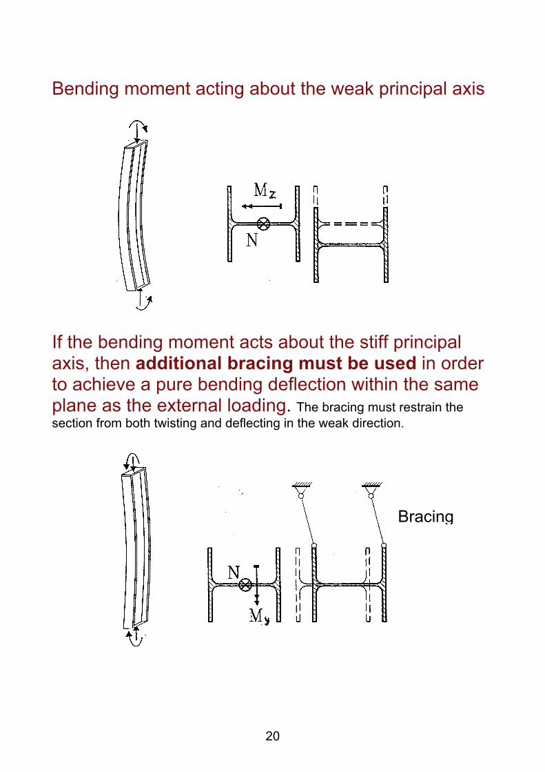
Bending moment acting about the weak principal axis

If the bending moment acts about the stiff principal axis, then additional bracing must be used in order to achieve a pure bending deflection within the same plane as the external loading. The bracing must restrain the section from both twisting and deflecting in the weak direction.

Bracing

21

Choosing the method of analysis for flexural buckling

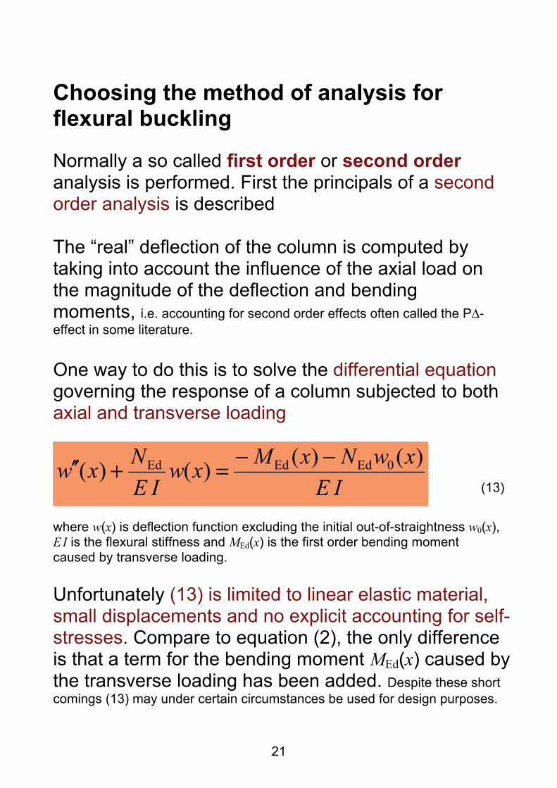
Normally a so called first order or second order analysis is performed. First the principals of a second order analysis is described The “real” deflection of the column is computed by taking into account the influence of the axial load on the magnitude of the deflection and bending moments, i.e. accounting for second order effects often called the PΔ-effect in some literature. One way to do this is to solve the differential equation governing the response of a column subjected to both axial and transverse loading

IExwNxMxw

IENxw )()()()( 0EdEdEd −−=+′′

(13)

where w(x) is deflection function excluding the initial out-of-straightness w0(x), E I is the flexural stiffness and MEd(x) is the first order bending moment caused by transverse loading.

Unfortunately (13) is limited to linear elastic material, small displacements and no explicit accounting for self-stresses. Compare to equation (2), the only difference is that a term for the bending moment MEd(x) caused by the transverse loading has been added. Despite these short comings (13) may under certain circumstances be used for design purposes.

22

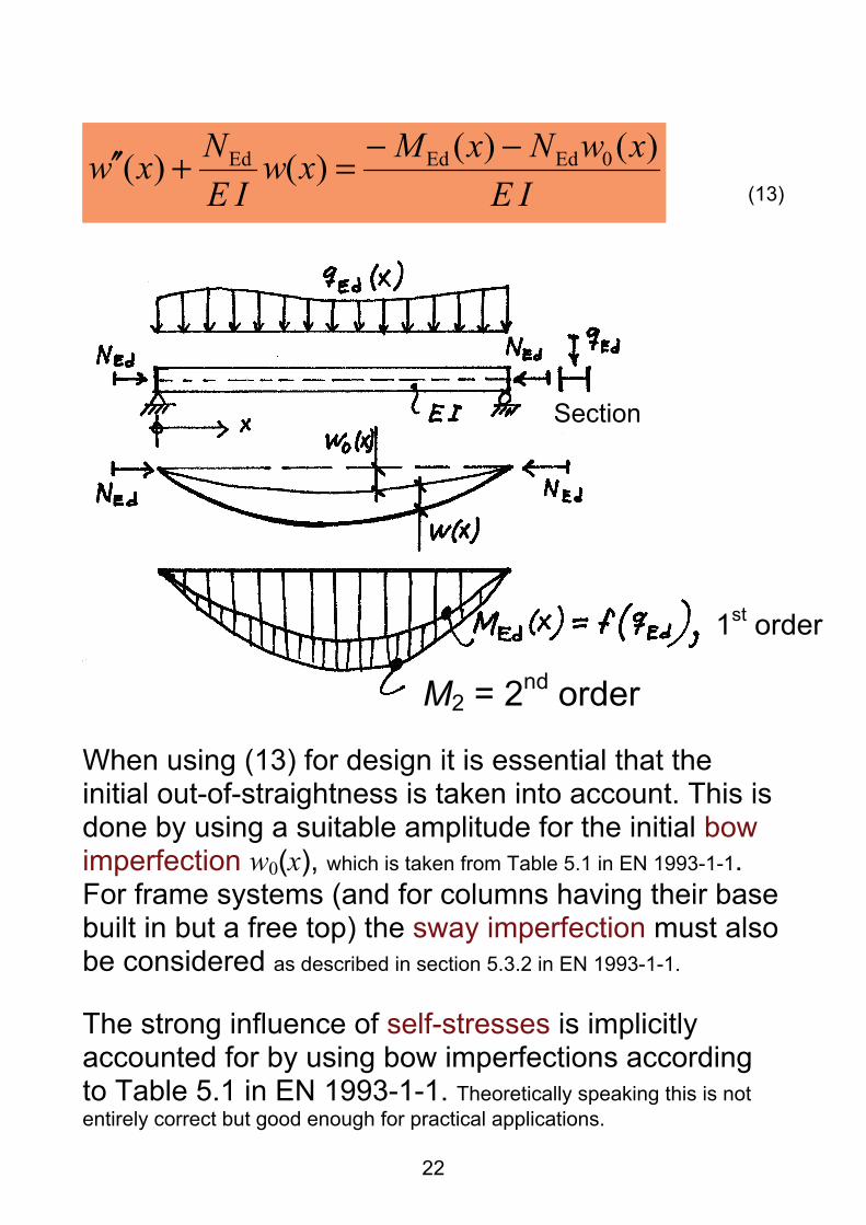
IExwNxMxw

IENxw )()()()( 0EdEdEd −−=+′′

(13)

When using (13) for design it is essential that the initial out-of-straightness is taken into account. This is done by using a suitable amplitude for the initial bow imperfection w0(x), which is taken from Table 5.1 in EN 1993-1-1. For frame systems (and for columns having their base built in but a free top) the sway imperfection must also be considered as described in section 5.3.2 in EN 1993-1-1.

The strong influence of self-stresses is implicitly accounted for by using bow imperfections according to Table 5.1 in EN 1993-1-1. Theoretically speaking this is not entirely correct but good enough for practical applications.

1st order

M2 = 2nd order

Section

23

Yet another drawback with (13) is that it actually requires linear elastic material where no yielding occurs. This is in a way also included in the fairly large initial bow imperfection stipulated by Table 5.1 in EN 1993-1-1. By using a too large bow imperfection, in relation to what would be needed for a linear elastic material, the plastic response in the failure region of the column is implicitly accounted for.

After the second order moment distribution has been found by solving (13) exactly or by some approximate method the resistance of the column is checked by an ordinary cross-sectional resistance check as described in Lectures 1 and 2.

The principals of a first order analysis The great advantage of this method is that the “real” second order deflection and corresponding bending moment need not be determined.

The second order effects are instead accounted for by using so called interaction relations according to section 6.3.3 in EN 1993-1-1 or by using a “general” first order approach according to section 6.3.4 in EN 1993-1-1.

24

Interaction relations according to section 6.3.3

Limitations:

• Double symmetric cross-sections.

• The cross-sectional shape may not change during loading, but section class 4 is ok.

• One must beside the interaction checks (6.61) or (6.62) also perform relevant cross-sectional checks at column ends, as described in Lectures 1 and 2 (section 6.2 in EN 1993-1-1). These later checks are not necessary if it is obvious that the interaction checks are more severe.

• The interaction formulae are derived for a simply supported beam having end fork boundary conditions with respect to torsion. But they may also be used for beam elements cut out from continuous beams and frame structures (cut out in between joints and/or supports).

• For single or multi story framed structures one must consider the second order effects very carefully. In case of pure flexural buckling this is usually done by using appropriate buckling lengths. But in case of lateral torsional buckling one may have to calculate the second order moment anyway.

25

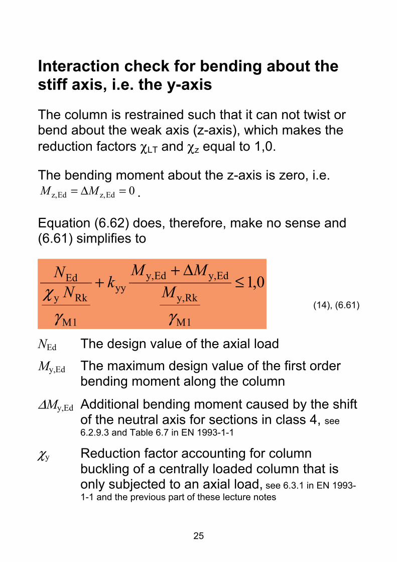
Interaction check for bending about the stiff axis, i.e. the y-axis

The column is restrained such that it can not twist or bend about the weak axis (z-axis), which makes the reduction factors χLT and χz equal to 1,0.

The bending moment about the z-axis is zero, i.e. 0Edz,Edz, =Δ= MM .

Equation (6.62) does, therefore, make no sense and (6.61) simplifies to

0,1

1M

Rky,

Edy,Edy,yy

1M

Rky

Ed ≤Δ+

+

γγχ M

MMkN

N

(14), (6.61)

NEd The design value of the axial load My,Ed The maximum design value of the first order

bending moment along the column

ΔMy,Ed Additional bending moment caused by the shift of the neutral axis for sections in class 4, see 6.2.9.3 and Table 6.7 in EN 1993-1-1

χy Reduction factor accounting for column buckling of a centrally loaded column that is only subjected to an axial load, see 6.3.1 in EN 1993-1-1 and the previous part of these lecture notes

26

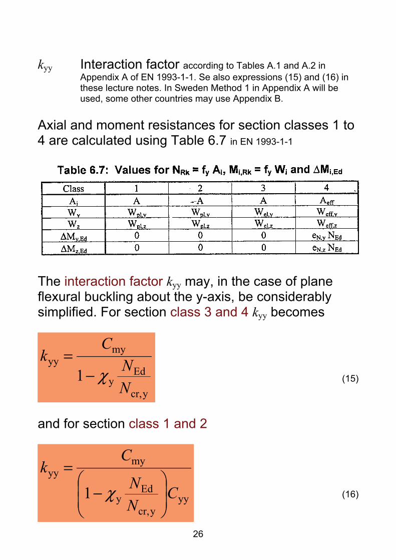
kyy Interaction factor according to Tables A.1 and A.2 in Appendix A of EN 1993-1-1. Se also expressions (15) and (16) in these lecture notes. In Sweden Method 1 in Appendix A will be used, some other countries may use Appendix B.

Axial and moment resistances for section classes 1 to 4 are calculated using Table 6.7 in EN 1993-1-1

The interaction factor kyy may, in the case of plane flexural buckling about the y-axis, be considerably simplified. For section class 3 and 4 kyy becomes

ycr,

Edy

myyy

1NN

Ck

χ−=

(15)

and for section class 1 and 2

yyycr,

Edy

myyy

1 CNN

Ck

⎟⎟⎠

⎞⎜⎜⎝

⎛−

=χ (16)

27

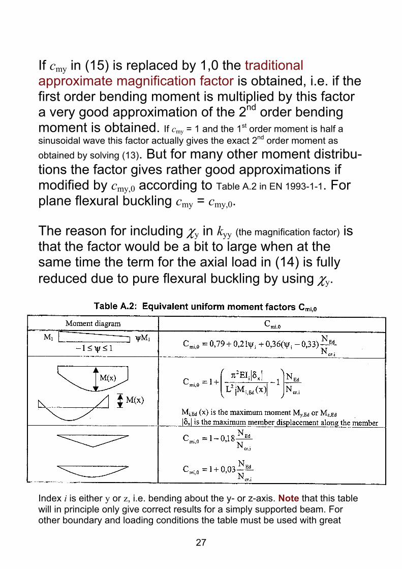
If cmy in (15) is replaced by 1,0 the traditional approximate magnification factor is obtained, i.e. if the first order bending moment is multiplied by this factor a very good approximation of the 2nd order bending moment is obtained. If cmy = 1 and the 1st order moment is half a sinusoidal wave this factor actually gives the exact 2nd order moment as obtained by solving (13). But for many other moment distribu-tions the factor gives rather good approximations if modified by cmy,0 according to Table A.2 in EN 1993-1-1. For plane flexural buckling cmy = cmy,0.

The reason for including χy in kyy (the magnification factor) is that the factor would be a bit to large when at the same time the term for the axial load in (14) is fully reduced due to pure flexural buckling by using χy.

Index i is either y or z, i.e. bending about the y- or z-axis. Note that this table will in principle only give correct results for a simply supported beam. For other boundary and loading conditions the table must be used with great

28

care. Setting cmi,0 to 1,0 is usually safe. Deriving the correct expression is also possible.

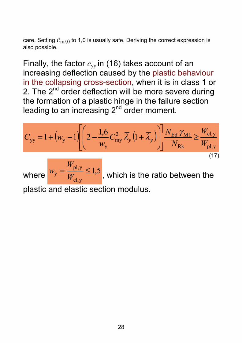
Finally, the factor cyy in (16) takes account of an

increasing deflection caused by the plastic behaviour in the collapsing cross-section, when it is in class 1 or 2. The 2nd order deflection will be more severe during the formation of a plastic hinge in the failure section leading to an increasing 2nd order moment.

( ) ( )ypl,

yel,

Rk

1MEd2my

yyyy 16,1211

WW

NNC

wwC yy ≥

⎥⎥⎦

⎤

⎢⎢⎣

⎡⎟⎟⎠

⎞⎜⎜⎝

⎛+−−+= γλλ

(17)

where 5,1yel,

ypl,y ≤=

WW

w , which is the ratio between the

plastic and elastic section modulus.

29

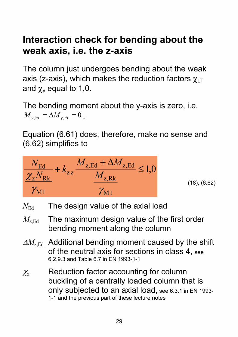
Interaction check for bending about the weak axis, i.e. the z-axis

The column just undergoes bending about the weak axis (z-axis), which makes the reduction factors χLT and χy equal to 1,0.

The bending moment about the y-axis is zero, i.e. ,Ed y,Ed 0yM M= Δ = .

Equation (6.61) does, therefore, make no sense and (6.62) simplifies to

0,1

1M

Rkz,

Edz,Edz,zz

1M

Rkz

Ed ≤Δ+

+

γγχ M

MMkN

N

(18), (6.62)

NEd The design value of the axial load Mz,Ed The maximum design value of the first order

bending moment along the column

ΔMz,Ed Additional bending moment caused by the shift of the neutral axis for sections in class 4, see 6.2.9.3 and Table 6.7 in EN 1993-1-1

χz Reduction factor accounting for column buckling of a centrally loaded column that is only subjected to an axial load, see 6.3.1 in EN 1993-1-1 and the previous part of these lecture notes

30

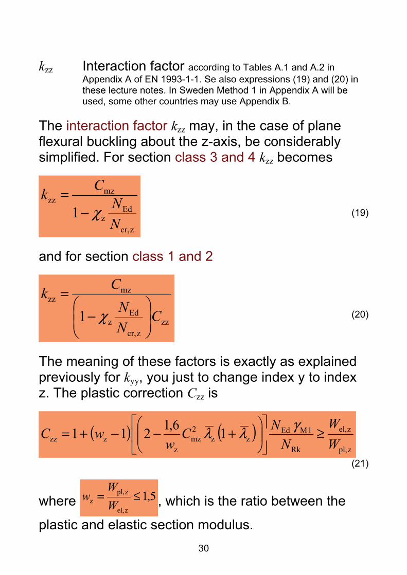
kzz Interaction factor according to Tables A.1 and A.2 in Appendix A of EN 1993-1-1. Se also expressions (19) and (20) in these lecture notes. In Sweden Method 1 in Appendix A will be used, some other countries may use Appendix B.

The interaction factor kzz may, in the case of plane flexural buckling about the z-axis, be considerably simplified. For section class 3 and 4 kzz becomes

zcr,

Edz

mzzz

1NN

Ckχ−

= (19)

and for section class 1 and 2

zzzcr,

Edz

mzzz

1 CNN

Ck

⎟⎟⎠

⎞⎜⎜⎝

⎛−

=χ (20)

The meaning of these factors is exactly as explained previously for kyy, you just to change index y to index z. The plastic correction Czz is

( ) ( )zpl,

zel,

Rk

1MEdzz

2mz

zzzz 16,1211

WW

NNC

wwC ≥⎥

⎦

⎤⎢⎣

⎡⎟⎟⎠

⎞⎜⎜⎝

⎛+−−+= γλλ

(21)

where 5,1zel,

zpl,z ≤=

WW

w , which is the ratio between the

plastic and elastic section modulus.

31

Using the “general” first order method

This method will not be used in this course. But if you want to use it you must study section 6.3.4 in EN 1993-1-1.

It is a simple and versatile method that is easy to use, but normally one must also use some computer based analysis tools in order to make the most out of the method. However, in simple cases, hand calculations are sufficient.