Lecture 2:More Time Integration and

Some Rigid BodiesJan 9, 2014

Today’s Plan

• A few more details on presentations/discussions

• Wrap up some slides from last time

• More on time integration

• Intro to rigid bodies

Presentation scheduling

First pair of presenters and papers for Thurs, Jan 16:

• Dominik: “Non-convex rigid bodies with stacking”

• Li: TBD

Remainder still to be determined. I’ve heard from 6 of you so far.

If you send me a draft of your slides 24-48 hours prior, I will try to provide some suggestions.

Presentations

A typical format is…

• Motivate the topic/problem

• Briefly outline key related work

• Describe the main contributions of the paper

• Show and discuss results• e.g. animations, graphs, comparisons to theory or experiment, etc.

• Provide a critique of the paper (both good and bad)

• Conclude briefly

Presentations - Tips

• Don’t explain every tiny detail – focus on core/novel contributions

• Prefer diagrams and images (and your voice) over lots of tiny text

• Avoid overwhelming with equations

• Talk to the audience, not the slides

• Do not recycle the authors slides. (Figures, graphs, results are fine.)

• Practice!

Analyzing a paper

Imagine you are a reviewer deciding whether to accept or reject…

Questions to ask yourself:• Did the authors clearly motivate the problem?

• Are the contributions truly novel wrt. previous work?

• How substantial are the contributions?

• Why did the authors make the [technical/design/theoretical] choices they did?

• Do the results actually achieve/support what was claimed?

• Are the writing and figures clear?

Reviews

See SIGGRAPH review format here:

http://s2013.siggraph.org/submitters/technical-papers/review-form

(Skip “reviewer expertise” and “private comments”)

Length: Aim for a few paragraphs.

MIT’s Fredo Durand has some tips for reviewing papers:• http://people.csail.mit.edu/fredo/review.pdf

Keshav offers some great strategies for reading papers (and more good references):

http://blizzard.cs.uwaterloo.ca/keshav/home/Papers/data/07/paper-reading.pdf

Discussions

• Everyone should read the papers and bring comments/questions/critiques.

• Bring a PDF or print-out to refer to.

• This is a good chance to dive further into technical details, things that remain unclear, debate the merit of the work, etc.

• Presenter can guide the discussion, but need not have all the answers.

Picking up from last time…

Recap:

• Time integration schemes (FE, RK2, …) enable us to solve for the evolution of a physical system, given the forces driving it.

• We discussed basic particle systems, identified some typical forces.

Forces

What physical forces might we use to drive a particle system?• Gravity• Wind• Springs / Elasticity• Damping / Viscosity• Friction• Collisions/Contact• …

Given the set of forces 𝐹1, 𝐹2, … , 𝐹𝑛, sum to get net force on a particle.

Forces: Damping/Viscosity

Often helpful to gradually slow the motion, avoid oscillating forever.

Approximates internal friction or energy dissipation.

Typically opposes the motion of the particle(s), and is proportional to the velocity. For example…

𝐹 = −𝑘𝑑𝑉

Note: Too much can look unrealistic/gooey.

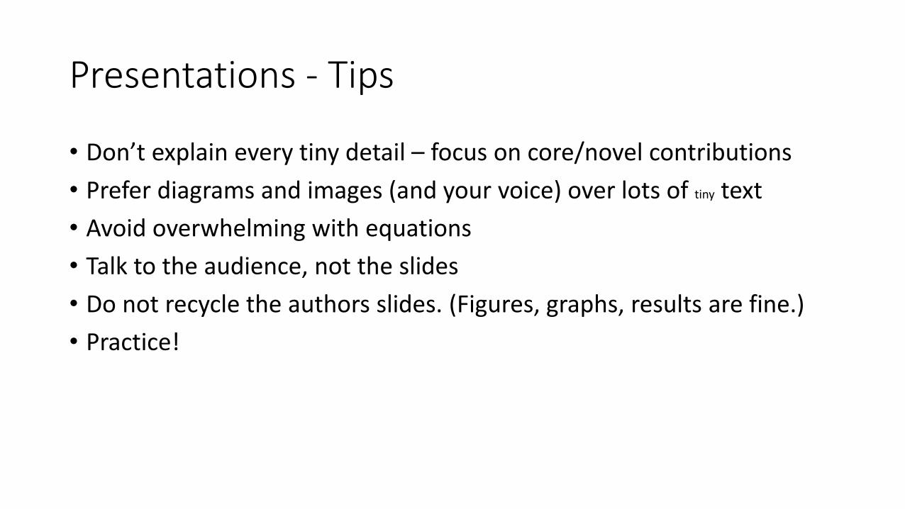
Forces: Normal & Friction (Contact forces)

Normal force: Resists interpenetration

Friction force: Resists relative sliding between materials.

Forces: Collisions

One strategy for modeling collisions is penalty/repulsion forces.

Essentially, temporary springs that oppose inter-penetration of objects.

Time Integration, Revisited

A Little More Time Integration

Last time:

• Forward Euler (FE) and Midpoint (RK2) schemes

• Numerical time integration introduces error

• Forward Euler (and similar) can sometimes blow up!

Today:

• A brief look at Forward Euler error and stability

• Implicit integration basics

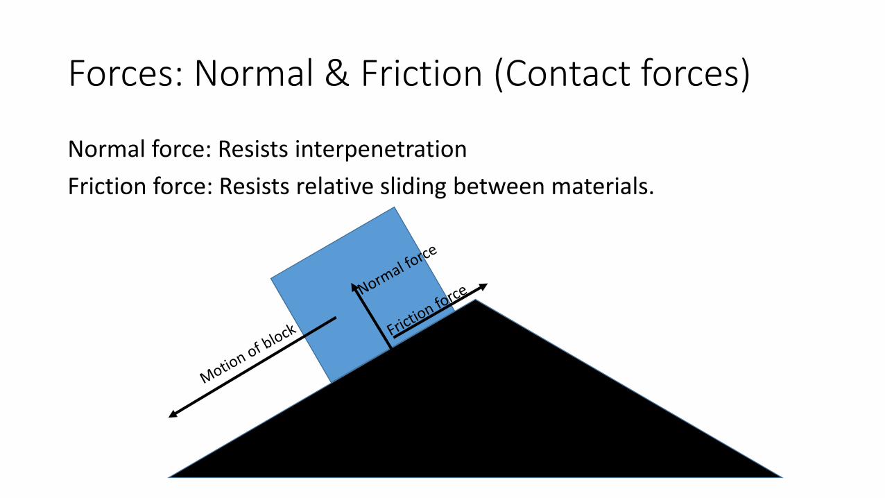
Error of Forward Euler

For dx/dt = V, forward Euler is:

𝑋(𝑡 + ∆𝑡) = 𝑋(𝑡) + 𝑉(𝑡)∆𝑡

How can we determine the error made in one step? 𝑋(𝑡)

𝑋(𝑡 + ∆𝑡)

Error of Forward Euler

What is the true solution at 𝑋(𝑡 + ∆𝑡)?

We don’t know it exactly, but we can approximate it with a Taylor series expansion:

𝑋 𝑡 + ∆𝑡 = 𝑋 𝑡 + ∆𝑡𝑋′ 𝑡 +∆𝑡2𝑋′′(𝑡)

2+ 𝑂(∆𝑡3)

Higher order terms, negligible for small ∆𝑡…

This is just velocity, V.

Error of Forward Euler

𝑋𝑡𝑟𝑢𝑒 𝑡 + ∆𝑡 = 𝑋 𝑡 + ∆𝑡𝑋′ 𝑡 +∆𝑡2𝑋′′(𝑡)

2+ 𝑂(∆𝑡3)

𝑋𝐹𝐸 𝑡 + ∆𝑡 = 𝑋 𝑡 + ∆𝑡𝑋′ 𝑡

The difference is called the local truncation error:

𝑋𝑡𝑟𝑢𝑒 − 𝑋𝐹𝐸 =∆𝑡2𝑋′′(𝑡)

2+ 𝑂(∆𝑡3)

Therefore the O ∆𝑡2 term dominates the error.

What about accumulated error?

What is the total error after 𝑛 steps, at time 𝑡𝑛 = 𝑡0 + 𝑛∆𝑡?

Each step incurs 𝑂 ∆𝑡2 error. To get to 𝑡𝑛 we take 𝑛 =𝑡𝑛−𝑡0

∆𝑡= 𝑂(

1

∆𝑡) steps.

The global error is thus 𝑂 ∆𝑡 , and we say Forward Euler is a 1st order accurate method.

• A more precise argument depends on properties of V itself.

Similarly, the midpoint method (RK2) is 2nd order.

Stability of Forward Euler

We saw that FE can blow up for large time steps, e.g. recall: 𝑑𝑥

𝑑𝑡= −𝑥.

So how large is too large?

Apply FE to the linear test equation:𝑑𝑥

𝑑𝑡= 𝜆𝑥

Result is: 𝑥𝑛+1 = 𝑥𝑛 + Δ𝑡𝜆𝑥𝑛 = 𝑥𝑛 1 + Δ𝑡𝜆

Behavior after many steps?

𝑥𝑛 = 𝑥0(1 + Δ𝑡𝜆)𝑛

Stability of Forward Euler

So, we have: 𝑥𝑛 = 𝑥0(1 + Δ𝑡𝜆)𝑛

When does it blow up (grow)? When does it decay?

For stability, we therefore need: 1 + Δ𝑡𝜆 < 1

This can be shown to imply: 0 < Δ𝑡 <2

|𝜆|

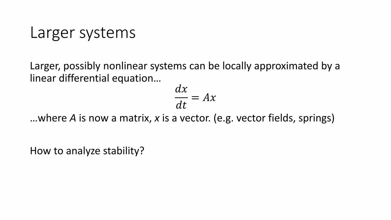
Larger systems

Larger, possibly nonlinear systems can be locally approximated by a linear differential equation…

𝑑𝑥

𝑑𝑡= 𝐴𝑥

…where A is now a matrix, x is a vector. (e.g. vector fields, springs)

How to analyze stability?

Matrix Eigenvalues

Recall: eigenvalues characterize how a matrix acts on corresponding eigenvectors.

𝐴𝑣 = 𝜆𝑣

By analyzing stability of each eigenvalue, 𝜆, independently, we can find timestep for the most restrictive “mode”.

Stability Regions

Eigenvalues of a problem may even be complex…

We can visualize the absolute region of stability on the complex plane, by plotting whether stability is satisfied for different values of the product Δ𝑡𝜆.

FE: 1 + Δ𝑡𝜆 < 1

Re

Im

Impact of Stability

Rotational/oscillatory motion corresponds to imaginary eigenvalues.

Often the stability restriction can be very (or impossibly!) limiting.

e.g. Rotational velocity fields, springs, etc.

FE: 1 + Δ𝑡𝜆 < 1

Imaginary Eigenvalues

Recall the rotational vector field V = (-y,x).

Then…𝑑

𝑑𝑡

𝑥𝑦 =

0 −11 0

𝑥𝑦

𝐴 =0 −11 0

has strictly imaginary eigenvalues, λ = ±𝑖.

Forward Euler is never stable here; stability region doesn’t include these points, which lie on the (vertical) imaginary axis.

Try a 1D spring, also.

Midpoint (AKA Runge Kutta 2) Runge Kutta 4(A similar 4th order scheme)

Stability Regions for other methods

Implicit (or backward) Euler

An alternative scheme is implicit Euler (or backward Euler).

Idea: use the (unknown!) velocity at the end of the timestep to approximate the integral.

Vel

oci

ty

t0 t1 = t0+∆t

v1

v0

Time

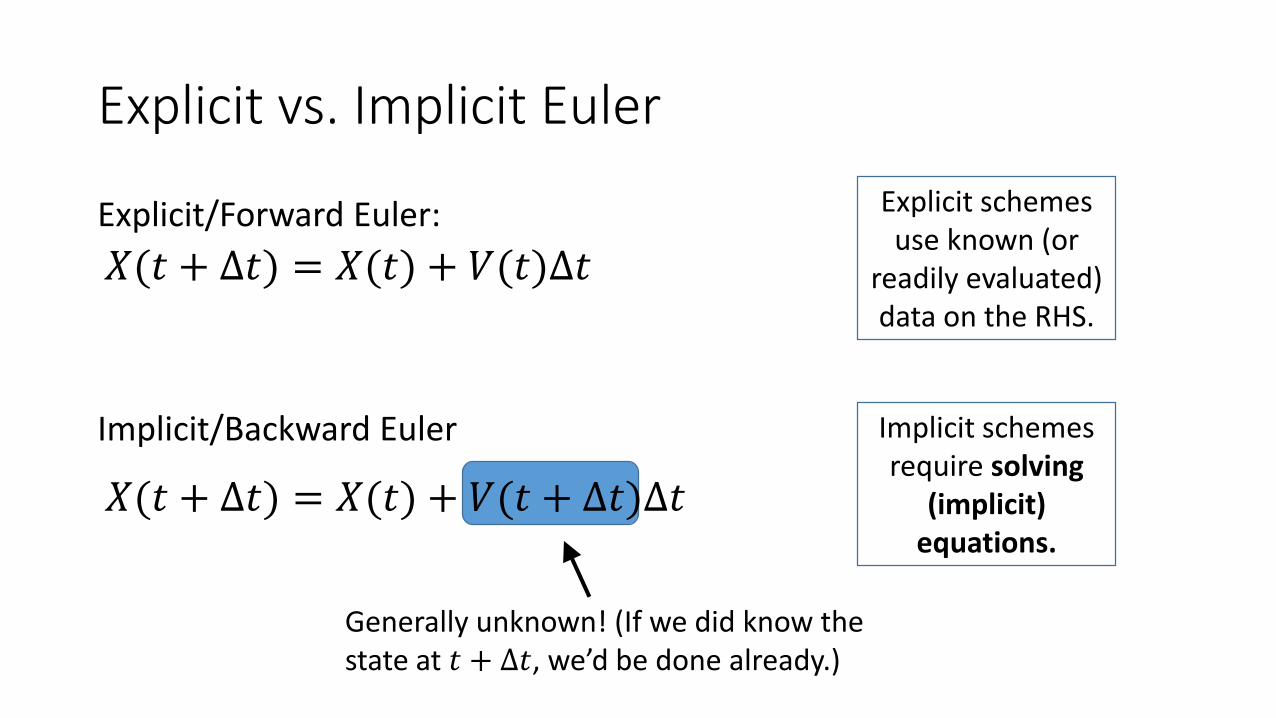
Explicit/Forward Euler:

Implicit/Backward Euler

Explicit vs. Implicit Euler

𝑋(𝑡 + ∆𝑡) = 𝑋(𝑡) + 𝑉(𝑡)∆𝑡

𝑋(𝑡 + ∆𝑡) = 𝑋(𝑡) + 𝑉(𝑡 + ∆𝑡)∆𝑡

Explicit schemes use known (or

readily evaluated) data on the RHS.

Implicit schemes require solving

(implicit) equations.

Generally unknown! (If we did know the state at 𝑡 + ∆𝑡, we’d be done already.)

Stability – Backward Euler

Consider our test equation again: 𝑑𝑥

𝑑𝑡= 𝜆𝑥

Backward Euler gives:𝑋 𝑡 + ∆𝑡 = 𝑋 𝑡 + 𝜆∆𝑡𝑋 𝑡 + ∆𝑡

This is an implicit equation for 𝑋 𝑡 + ∆𝑡 .

So we have to solve for it, in this case by rearranging:

𝑋 𝑡 + ∆𝑡 =𝑋 𝑡

1 − 𝜆∆𝑡

Stability – Backward Euler

For a single step:

𝑋 𝑡 + ∆𝑡 =𝑋 𝑡

1 − 𝜆∆𝑡

So for step n, we have:

𝑋𝑛 =𝑋0

(1 − 𝜆Δ𝑡)𝑛

When does this decay? (i.e. when is it stable?)1 − 𝜆Δ𝑡 ≥ 1

Stability Regions – Explicit vs. Implicit Euler

1 − 𝜆Δ𝑡 ≥ 11 + 𝜆Δ𝑡 ≤ 1

Implicit Euler

Can sometimes behave stably even when the “physics”/problem is not!

e.g.,𝑑𝑥

𝑑𝑡= 𝑥

Solution is 𝑒𝑡, which grows exponentially.

(Imagine a physical system that gains speed exponentially.)

This corresponds to the right half of the complex plane.

BE gives:

𝑋𝑛 =𝑋0

(1 − Δ𝑡)𝑛

If you take large steps, the numerical solution will decay in magnitude, which doesn’t match the true solution!

Implicit Euler

In practice:

• BE is stable for large time steps.

• The price is overly damped motion (rapid loss of energy).

For problems with multiple variables, need to solve a linear system of equations. (See CS370,CS475)

This system may also be non-linear…• Need to iterate, using Newton’s method or other nonlinear solver.• Typically requires computing derivatives of the functions/forces.

Trapezoidal rule

Other schemes mix explicit and implicit integration.

Trapezoidal rule is half a step of FE, half a step of BE!

Stable when the “physics” is.

i.e., the left half of the complex plane.

𝑋(𝑡 + ∆𝑡) = 𝑋(𝑡) + ∆𝑡𝑉(𝑡)+ 𝑉(𝑡 + ∆𝑡)

2

Caveat…

Technically, these stability analyses only apply to linear problems.

But, they are often indicative of behaviour for nonlinear problems too.

Rigid Bodies

Rigid Bodies

For modeling very stiff objects, a mass-spring/deformable system is problematic… Why?

• Explicit methods, will need very small time steps.

• Implicit methods, equations become ill-conditioned (hard to solve)

• Deformation happens fast, but is not the (visually) interesting part!

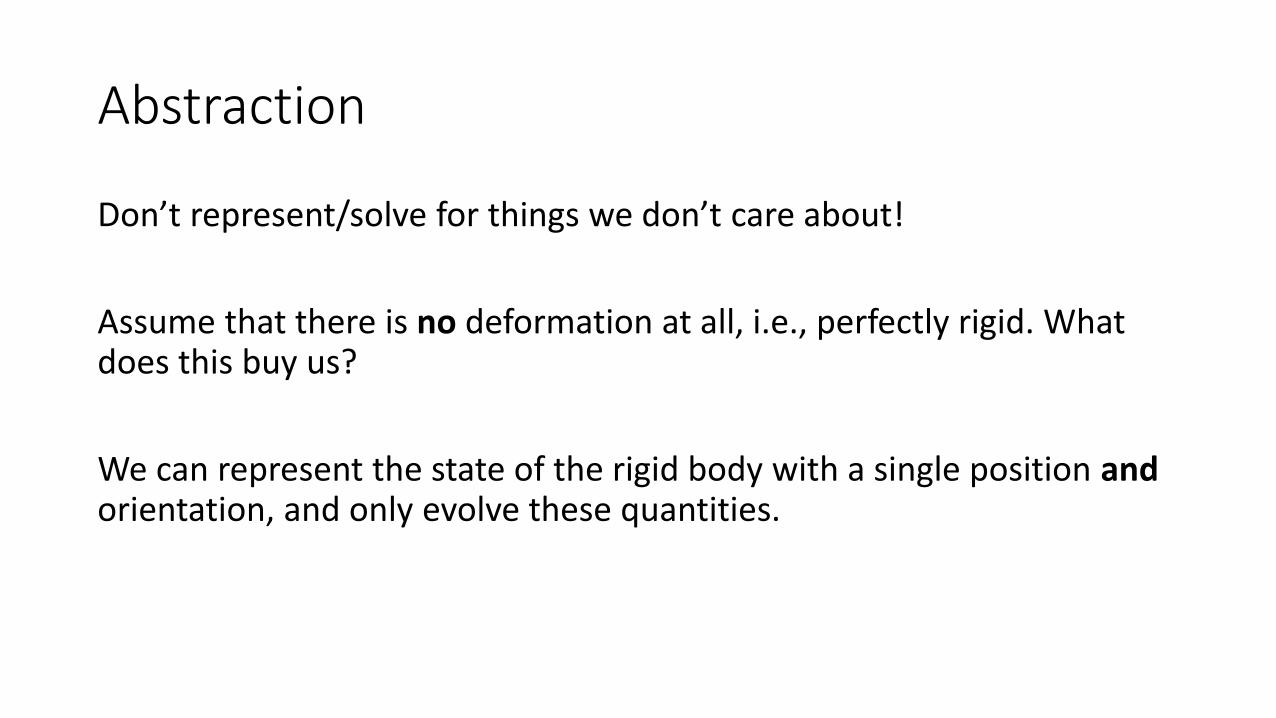
Abstraction

Don’t represent/solve for things we don’t care about!

Assume that there is no deformation at all, i.e., perfectly rigid. What does this buy us?

We can represent the state of the rigid body with a single position andorientation, and only evolve these quantities.

Rigid body state

Rigid body state

We can use a standard affine transformation to represent the position and orientation of the body at any time.For any point on the body, we can find its current position in world space.

Body space

World space

Points on the rigid body

If:

• 𝑝0 is the 3D position of a point in body space

• centre of mass is the 3D position vector, c(t)

• orientation is represented by a rotation matrix, R(t)

Then current world position of the particle, p(t) is:𝑝 𝑡 = 𝑐 𝑡 + 𝑅 𝑡 𝑝0

Evolving Position – Easy!

Treat the centre of mass of the object as a single point/particle, having the full mass of the rigid body.

Solve the usual equations of motion for position and velocity:𝑑

𝑑𝑡𝑋𝑉

=𝑉

𝐹/𝑀

How do we evolve the orientation?

Representing Orientation

Representation can be important…

2D: a single angle

3D: • Euler angles (1 angle per axis). (Suffers from “gimbal lock”.)

• 3x3 rotation matrices, R. (We’ll use these for simplicity, but suffer from drift).

• Quaternions are common in practice. (See the Baraff/Witkin notes for more.)

Main question: What are the corresponding equations of motion for orientation? i.e., How does R evolve?

𝑑

𝑑𝑡𝑅?

=??

𝑑

𝑑𝑡𝑋𝑉

=𝑉

𝐹/𝑀

Position: Orientation:

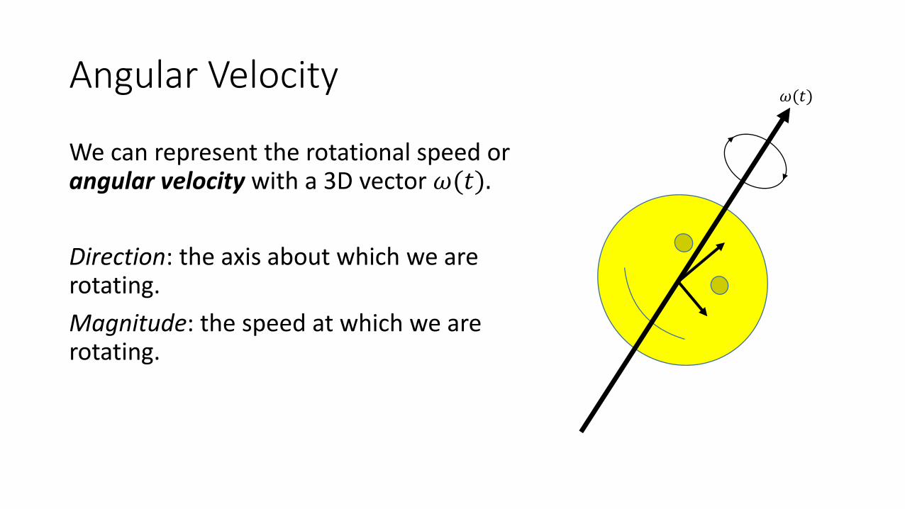
Angular Velocity

We can represent the rotational speed or angular velocity with a 3D vector 𝜔(𝑡).

Direction: the axis about which we are rotating.

Magnitude: the speed at which we are rotating.

𝜔(𝑡)

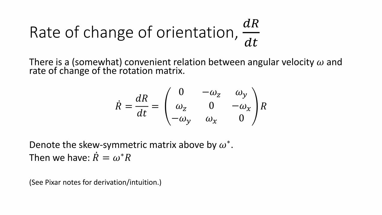
Rate of change of orientation, 𝑑𝑅

𝑑𝑡

There is a (somewhat) convenient relation between angular velocity 𝜔 and rate of change of the rotation matrix.

𝑅 =𝑑𝑅

𝑑𝑡=

0 −𝜔𝑧 𝜔𝑦

𝜔𝑧 0 −𝜔𝑥

−𝜔𝑦 𝜔𝑥 0𝑅

Denote the skew-symmetric matrix above by 𝜔∗.Then we have: 𝑅 = 𝜔∗𝑅

(See Pixar notes for derivation/intuition.)

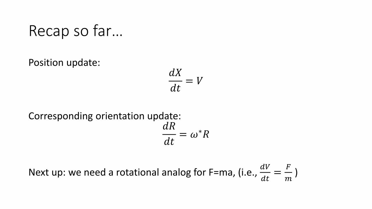
Recap so far…

Position update:𝑑𝑋

𝑑𝑡= 𝑉

Corresponding orientation update:𝑑𝑅

𝑑𝑡= 𝜔∗𝑅

Next up: we need a rotational analog for F=ma, (i.e., 𝑑𝑉

𝑑𝑡=

𝐹

𝑚)

Torque

Torque, 𝜏, is the rotational analog of force.

It is computed as:𝜏 = 𝑟 − 𝑐 × 𝐹

for a force F applied at a point 𝑟on the rigid body, where 𝑐 is the centre of mass.

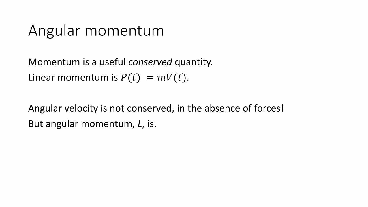
Angular momentum

Momentum is a useful conserved quantity.

Linear momentum is 𝑃(𝑡) = 𝑚𝑉(𝑡).

Angular velocity is not conserved, in the absence of forces!

But angular momentum, L, is.

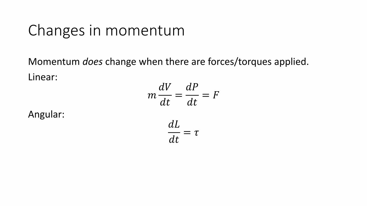
Changes in momentum

Momentum does change when there are forces/torques applied.

Linear:

𝑚𝑑𝑉

𝑑𝑡=𝑑𝑃

𝑑𝑡= 𝐹

Angular: 𝑑𝐿

𝑑𝑡= 𝜏

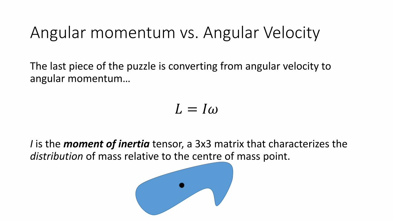
Angular momentum vs. Angular Velocity

The last piece of the puzzle is converting from angular velocity to angular momentum…

𝐿 = 𝐼𝜔

I is the moment of inertia tensor, a 3x3 matrix that characterizes the distribution of mass relative to the centre of mass point.

Inertia Tensor I

The rotational counterpart of mass. (Compare 𝐿 = 𝐼𝜔 vs. P = 𝑚𝑉)

Mass of the rigid body is the integral of density 𝑚 = 𝜌 𝑑𝑉 over the body.

Moment of inertia is also an integral:

𝐼 = 𝜌

𝑟𝑦2 + 𝑟𝑧

2 𝑟𝑥𝑟𝑦 𝑟𝑥𝑟𝑧

𝑟𝑥𝑟𝑦 𝑟𝑥2 + 𝑟𝑧

2 𝑟𝑦𝑟𝑧

𝑟𝑥𝑟𝑧 𝑟𝑦𝑟𝑧 𝑟𝑥2 + 𝑟𝑦

2

𝑑𝑉

For many common shapes, simple formulas exist.

Inertia Tensor I

Subtlety: the current inertia tensor I(t) in world space changes over time!

Re-computing at each step would be costly…

Fortunately, it can be shown that:𝐼 𝑡 = 𝑅 𝑡 𝐼𝑏𝑜𝑑𝑦𝑅 𝑡 𝑇

(See Pixar notes for a derivation.)

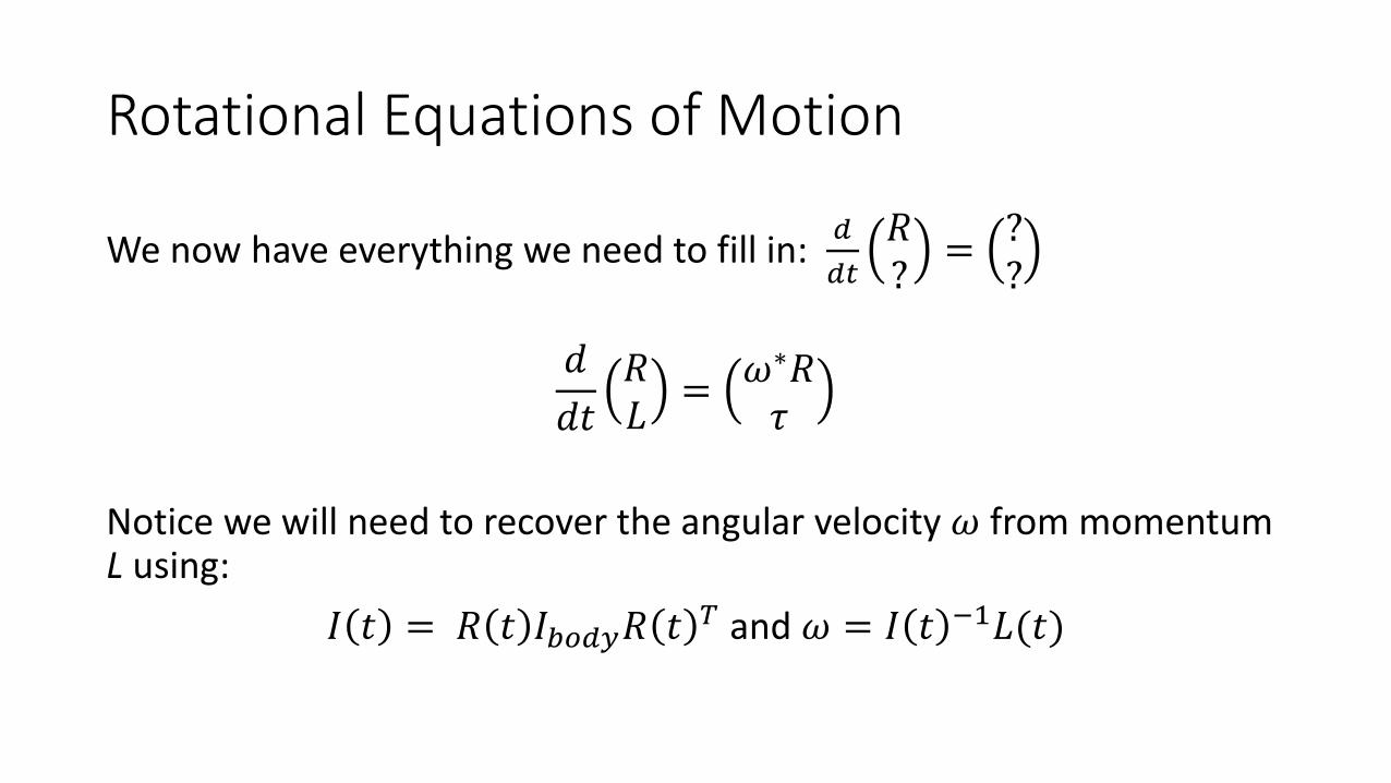
Rotational Equations of Motion

We now have everything we need to fill in: 𝑑

𝑑𝑡

𝑅?

=??

𝑑

𝑑𝑡𝑅𝐿

=𝜔∗𝑅𝜏

Notice we will need to recover the angular velocity 𝜔 from momentum L using:

𝐼 𝑡 = 𝑅 𝑡 𝐼𝑏𝑜𝑑𝑦𝑅 𝑡 𝑇 and 𝜔 = 𝐼 𝑡 −1𝐿(𝑡)

Analogy between position and orientation:

Position variables:𝑑𝑋

𝑑𝑡= 𝑉

𝑚𝑑𝑉

𝑑𝑡=

𝑑𝑃

𝑑𝑡= 𝐹

𝑃 = 𝑚𝑉

Orientation variables:𝑑𝑅

𝑑𝑡= 𝜔∗𝑅

𝑑𝐿

𝑑𝑡= 𝜏

𝐿 = 𝐼𝜔

Time integration

Apply your favourite time integration scheme to this full set of equations. (Forward Euler, midpoint, etc.)

Try writing out the steps for forward Euler on a rigid body.

Collisions

Two main families, typically.

• Penalty/repulsion methods (briefly, last time)

• Impulse methods (briefly, this time)

Penalty method applies force over some period of contact, ∆𝑡.

Impulses are an instantaneous application of force over an infinitesimal period, i.e., conceptual limit as ∆𝑡 → 0.

Impulses – Elastic Collisions

Consider a rubber ball falling onto a ground plane. How must the (vertical) velocity change for the ball to bounce perfectly?

𝑉𝑦 = −1 𝑉𝑦 = +1

We just reflect the (normal component of) velocity.

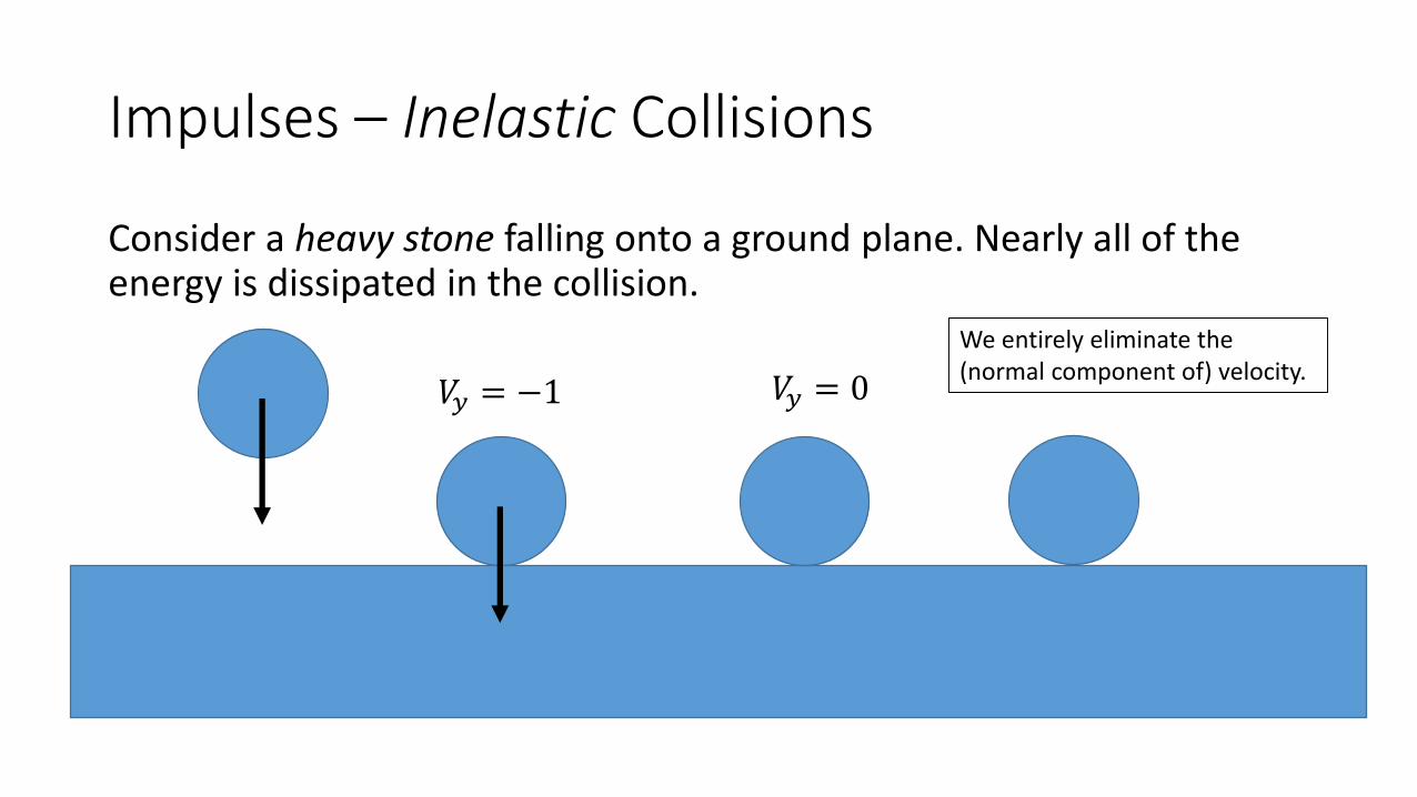
Impulses – Inelastic Collisions

Consider a heavy stone falling onto a ground plane. Nearly all of the energy is dissipated in the collision.

𝑉𝑦 = −1 𝑉𝑦 = 0

We entirely eliminate the(normal component of) velocity.

Coefficient of Restitution

Most collisions are somewhere between.

Coefficient of restitution, 𝜖 ∈ [0,1], models the fraction of energy remaining after a collision. Putting it together…

𝑉𝑟𝑒𝑙,𝑛𝑎𝑓𝑡𝑒𝑟

= −𝜖𝑉𝑟𝑒𝑙,𝑛𝑏𝑒𝑓𝑜𝑟𝑒

Note! Only the (relative) velocity in the normal direction changes.Tangential velocity is left alone (unless you add friction…)

See: “Nonconvex Rigid Bodies with Stacking” [Guendelman 2003] for a summary of the general case, with friction and rotational impulses.

Some Recent Examples

• Drawn from [Kaufman et al. 2008] and [Smith et al. 2012], on our papers list.

Physics-Based Animation

If you’re interested in following recent/new research, check out:

www.physicsbasedanimation.com

Where did that come from?

Consider how an arbitrary vector 𝑟(𝑡) is affected by the rotation.

Split 𝑟(𝑡) into perpendicular ⊥ and parallel ∥components, 𝑎 and 𝑏.

𝑟(𝑡) sweeps out a circle with radius 𝑏 .

The tip velocity is 𝜔(𝑡) × 𝑏.

But 𝜔 𝑡 ∥ 𝑎, so 𝜔 𝑡 × 𝑎 = 0.

Thus… 𝑟 = 𝜔 × 𝑎 + 𝑏 = 𝜔 × 𝑟

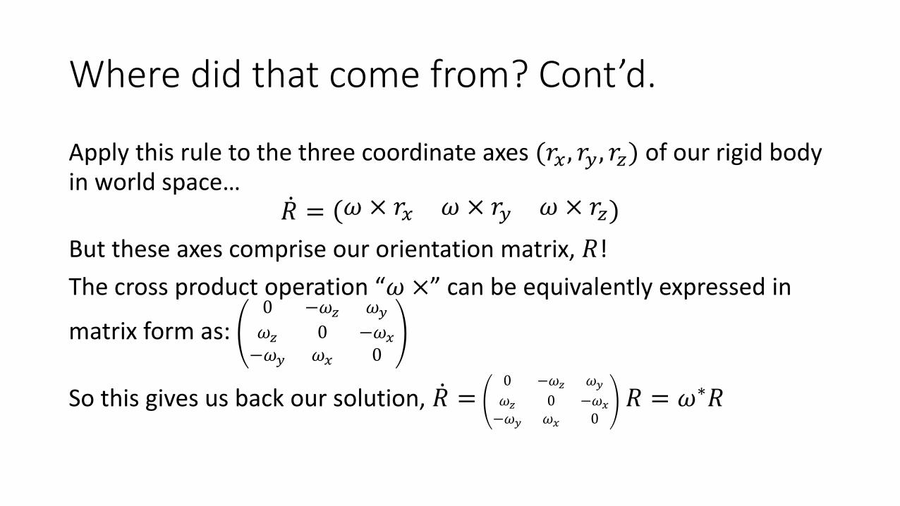
Where did that come from? Cont’d.

Apply this rule to the three coordinate axes (𝑟𝑥 , 𝑟𝑦 , 𝑟𝑧) of our rigid body in world space…

𝑅 = 𝜔 × 𝑟𝑥 𝜔 × 𝑟𝑦 𝜔 × 𝑟𝑧

But these axes comprise our orientation matrix, 𝑅!

The cross product operation “𝜔 ×” can be equivalently expressed in

matrix form as: 0 −𝜔𝑧 𝜔𝑦

𝜔𝑧 0 −𝜔𝑥

−𝜔𝑦 𝜔𝑥 0

So this gives us back our solution, 𝑅 =0 −𝜔𝑧 𝜔𝑦

𝜔𝑧 0 −𝜔𝑥

−𝜔𝑦 𝜔𝑥 0𝑅 = 𝜔∗𝑅