CS888 Lecture 2:More Time Integration and

Some Rigid BodiesJan 6, 2016

Reminder: Time Slot selection

I’ve created an online sign-up sheet:

http://www.slyreply.com/app/sheets/vr72g87b8q9j/

Please pick a date from the given list.

If you select a paper too, state it in the comment section, and ensure that it correspond to the topic for that week (rigid bodies, deformables, cloth, etc.)

I may juggle the order slightly (within topics) if it makes more sense.

Last time…

Recap:

• Time integration schemes (FE, RK2, …) enable us to solve for the evolution of a physical system, given the forces driving it.

• We discussed basic particle systems, identified some typical forces.

Plan

• Wrap up mass-springs intro, mention a couple more common forces.

• Further explore time integration and stability.

• Start on rigid bodies.

Hooke’s Law for 3D springs

For a spring joining 2 particles with position vectors 𝑋1 and 𝑋2:

𝐹1 = −𝐹2 = −𝑘( 𝑋1 − 𝑋2 − 𝐿)𝑋1 − 𝑋2𝑋1 − 𝑋2

Direction

Displacement𝑋1

𝑋2

𝑋1

𝑋2

𝐿

𝐹1

𝐹2

Rest state:

Stretched state:

Springs for Hair

A single chain of masses and springs can model stretching of a strand of hair.

What about bending?

Springs for Hair

Simple model: Add alternating springs. This discourages the hair from collapsing when you bend it.

What about twisting?See “A Mass Spring Model for Hair Simulation” [Selle et al. 2008]

[Selle et al. 2008]

Springs for Cloth

Using a grid of particles, a similar approach has been used to model cloth.

• Red springs model stretching/shearing.

• Blue springs model bending.

From “Stable but responsive cloth”, Choi and Ko, 2002.

From “Robust treatment of collisions, contact and friction for cloth animation”, Bridson et al. 2002

Springs for 3D Deformables

3D networks of springs form a simple model for volumetric deformable objects (AKA “soft body dynamics”).

• Typically connected in a mesh of

tetrahedra or hexahedra.

E.g.

A volumetric mass-spring animation[Selle et al. 2008]

For cloth/shells, can we control stretching and bending strength independently?

No! “Bending” springs also affect stretchiness in a non-trivial way.

Problems with springs…

If we double the cloth mesh resolution (particle density), will the behaviourbe consistent?

No! Ideally, the motion should approach some “true” solution as we refine. In general, simple mass-spring system do not converge.

More consistent finite difference, finite element, or finite volume approaches are preferred in VFX, and some games have gone this way too.

Problems with springs…

More Forces: Damping/Viscosity

Approximates internal friction or energy dissipation (to heat).

Gradually slows the motion; avoids oscillating forever.

Damping typically… (1) opposes the motion of the system, and (2) is proportional to velocity. For example…

𝐹 = −𝑘𝑑𝑉

with the damping coefficient 𝑘𝑑.

Notice similarity to 1D spring force, 𝐹 = −𝑘Δ𝑥.

Too much damping can sometimes look unrealistic/gooey.Source Link

More Forces: Collisions

One strategy to handle collisions is penalty/repulsion forces.

Essentially, temporary springs that oppose inter-penetration of objects.

More Forces: Contact & Friction

Normal contact force: Resists interpenetration.

Friction force: Resists relative sliding between materials.

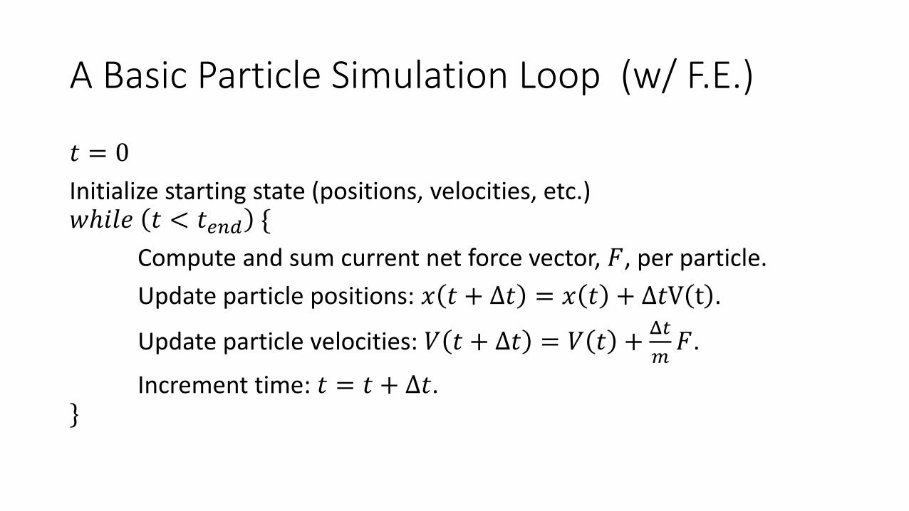
A Basic Particle Simulation Loop (w/ F.E.)

𝑡 = 0

Initialize starting state (positions, velocities, etc.)𝑤ℎ𝑖𝑙𝑒 𝑡 < 𝑡𝑒𝑛𝑑 {

Compute and sum current net force vector, 𝐹, per particle.

Update particle positions: 𝑥 𝑡 + Δ𝑡 = 𝑥 𝑡 + Δ𝑡V t .

Update particle velocities: 𝑉 𝑡 + Δ𝑡 = 𝑉 𝑡 +Δ𝑡

𝑚𝐹.

Increment time: 𝑡 = 𝑡 + Δ𝑡.}

Time Integration, Continued

A Little More Time Integration

Last time:

• Forward Euler (FE) and Midpoint (RK2) schemes

• Numerical time integration introduces error

• Forward Euler (and similar) can sometimes blow up!

Today:

• A brief look at Forward Euler error and stability

• Implicit integration basics

Error of Forward Euler

For 𝑑𝑥

𝑑𝑡= 𝑉, forward Euler is:

𝑋(𝑡 + ∆𝑡) = 𝑋(𝑡) + 𝑉(𝑡)∆𝑡

What is the error accumulated over one step? 𝑋(𝑡) 𝑋(𝑡 + ∆𝑡)

Numerical solution

True solution

Time 𝑡

Position 𝑋

Error

Error of Forward Euler

What is the true solution at 𝑋(𝑡 + ∆𝑡)?

We don’t know it exactly, but we can approximate it with a Taylor series expansion:

𝑋𝑡𝑟𝑢𝑒 𝑡 + ∆𝑡 = 𝑋 𝑡 + ∆𝑡𝑋′ 𝑡 +

∆𝑡2𝑋′′(𝑡)

2+ 𝑂(∆𝑡3)

Higher order terms, negligible for small ∆𝑡…

This is just velocity, V.

Error of Forward Euler

𝑋𝑡𝑟𝑢𝑒 𝑡 + ∆𝑡 = 𝑋 𝑡 + ∆𝑡𝑋′ 𝑡 +

∆𝑡2𝑋′′(𝑡)

2+ 𝑂(∆𝑡3)

𝑋𝐹𝐸 𝑡 + ∆𝑡 = 𝑋 𝑡 + ∆𝑡𝑋′ 𝑡

The difference is called the local truncation error:

𝑋𝑡𝑟𝑢𝑒 − 𝑋𝐹𝐸 =∆𝑡2𝑋′′(𝑡)

2+ 𝑂(∆𝑡3)

For small Δ𝑡, the O ∆𝑡2 term dominates the error.

How does error accumulate?

What is the total error after 𝑛 steps, at time 𝑡𝑛 = 𝑡0 + 𝑛∆𝑡?

Each step incurs 𝑂 ∆𝑡2 error. To get to 𝑡𝑛 we take 𝑛 =𝑡𝑛−𝑡0

∆𝑡= 𝑂

1

∆𝑡steps.

The product gives a global error of 𝑂 ∆𝑡 ; we say Forward Euler is 1st

order accurate. (Rigourous analysis depends on properties of V itself.)

Meaning: Halving Δ𝑡 should reduce observed error by a factor of 2.

FE v.s. RK2

Forward Euler error is 1st order, 𝑂 Δ𝑡 .

RungeKutta2 (explicit midpoint) is 2nd order, 𝑂 Δ𝑡2 .

→RK2 is asymptotically more accurate, i.e. approaches the exact solution faster as the timestep is reduced (“under refinement”).

Stability of Forward Euler

FE can “blow up” for large time steps, e.g. recall: 𝑑𝑥

𝑑𝑡= −𝑥.

So how large is too large?

Apply FE to the 1D linear test equation:𝑑𝑥

𝑑𝑡= 𝜆𝑥

Result is: 𝑥𝑛+1 = 𝑥𝑛 + Δ𝑡𝜆𝑥𝑛 = 𝑥𝑛 1 + Δ𝑡𝜆

Behaviour after many steps starting with 𝑥0?

𝑥𝑛 = 𝑥0(1 + Δ𝑡𝜆)𝑛

Stability of Forward Euler

So, we have: 𝑥𝑛 = 𝑥0(1 + Δ𝑡𝜆)𝑛

When does this blow up (increase exponentially)? When does it decay?

For stability, we therefore need: 1 + Δ𝑡𝜆 < 1

(Assuming 𝜆 is real and negative…) this implies: 0 < Δ𝑡 <2

|𝜆|.

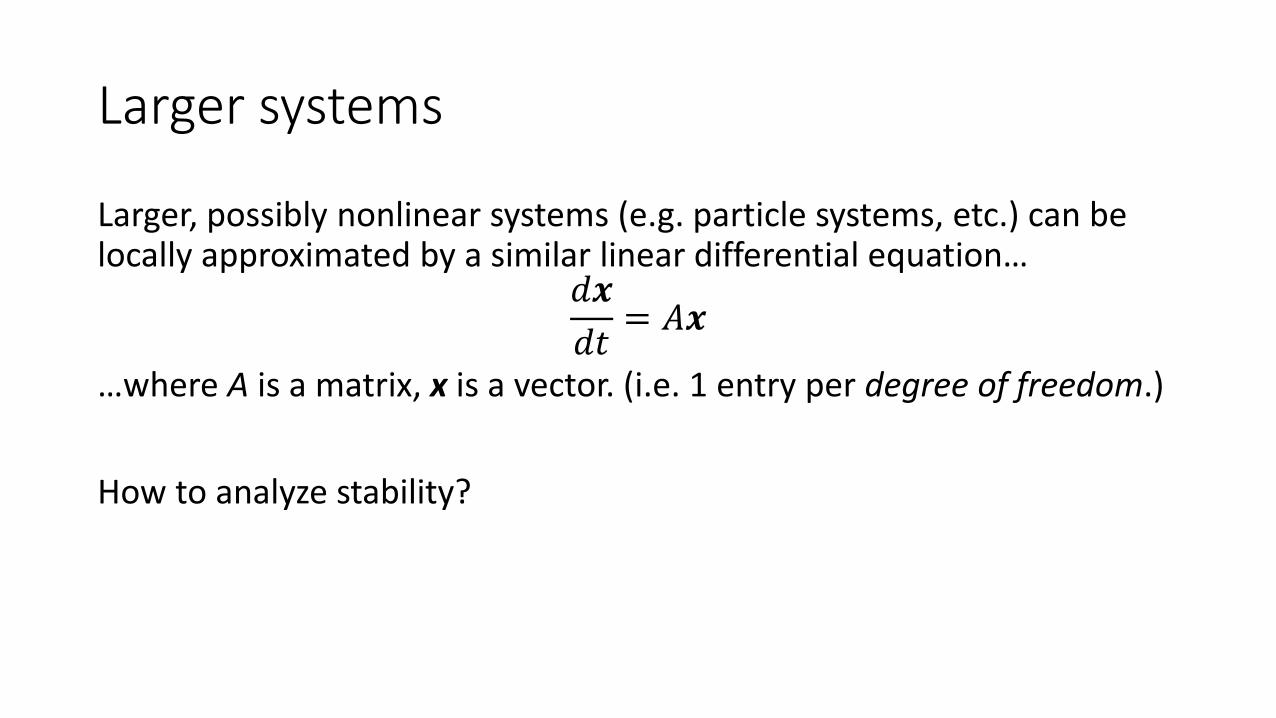
Larger systems

Larger, possibly nonlinear systems (e.g. particle systems, etc.) can be locally approximated by a similar linear differential equation…

𝑑𝒙

𝑑𝑡= 𝐴𝒙

…where A is a matrix, x is a vector. (i.e. 1 entry per degree of freedom.)

How to analyze stability?

Matrix Eigenvalues

Eigenvalues characterize how a matrix 𝐴 acts on corresponding eigenvectors 𝑣.

𝐴𝑣 = 𝜆𝑣

By analyzing stability of each eigenvalue, 𝜆, independently, we can find a stable timestep for the most restrictive “mode”.

Stability Regions

Eigenvalues of a problem can be complexnumbers…

We visualize the absolute region of stability on the complex plane, by plotting where the stability criterion is satisfied (by the product Δ𝑡𝜆.)

FE: 1 + Δ𝑡𝜆 < 1

Re

Im

Forward Euler stability region

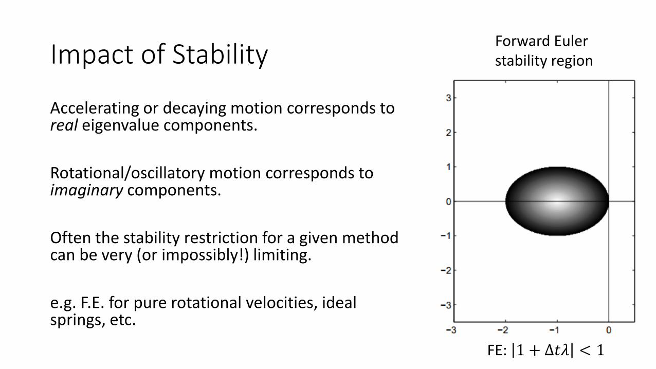
Impact of Stability

Accelerating or decaying motion corresponds to real eigenvalue components.

Rotational/oscillatory motion corresponds to imaginary components.

Often the stability restriction for a given method can be very (or impossibly!) limiting.

e.g. F.E. for pure rotational velocities, ideal springs, etc.

FE: 1 + Δ𝑡𝜆 < 1

Forward Euler stability region

Imaginary Eigenvalues

Recall the rotational vector field 𝑉 = (−𝑦, 𝑥).

The differential equation is…𝑑

𝑑𝑡

𝑥𝑦 =

0 −11 0

𝑥𝑦

The matrix 𝐴 =0 −11 0

has strictly imaginary

eigenvalues, λ = ±𝑖.

Imaginary eigenvalues

If λ = ±𝑖, where does Δ𝑡𝜆 lie in this picture?

On the imaginary axis, outside the stability region.

F.E. is never stable on purely rotational motion!

Likewise, for a purely oscillating 1D mass-spring:𝑑

𝑑𝑡

𝑥𝑉=

0 1−𝑘/𝑚 0

𝑥𝑉

FE: 1 + Δ𝑡𝜆 < 1

Forward Euler stability region

Midpoint (AKA Runge Kutta 2) Runge Kutta 4(A similar 4th order scheme)

Stability Regions for other (explicit) methods

Notice parts of the imaginary axis are included here.

Implicit (or backward) Euler

Another alternative scheme is implicit Euler (or backward Euler).

Idea: use the (unknown!) velocity at the end of the timestep to approximate the integral.

Vel

oci

ty

t0 t1 = t0+∆t

v1

v0

Time

Explicit/Forward Euler:

Implicit/Backward Euler

Compare: Explicit vs. Implicit Euler

𝑋(𝑡 + ∆𝑡) = 𝑋(𝑡) + 𝑉(𝑡)∆𝑡

𝑋(𝑡 + ∆𝑡) = 𝑋(𝑡) + 𝑉(𝑡 + ∆𝑡)∆𝑡

Explicit schemes use known (or

readily evaluated) data on the RHS.

Implicit schemes require solving

(implicit) equations.

Generally unknown. (If we knew the state at 𝑡 + ∆𝑡, we’d be done already!)

Stability – Backward Euler

Consider our test equation again: 𝑑𝑥

𝑑𝑡= 𝜆𝑥

Applying Backward Euler gives:𝑋 𝑡 + ∆𝑡 = 𝑋 𝑡 + 𝜆∆𝑡𝑋 𝑡 + ∆𝑡

This is an implicit equation for 𝑋 𝑡 + ∆𝑡 . i.e. it appears on both sides.

So we have to solve for it, in this case by rearranging:

𝑋 𝑡 + ∆𝑡 =𝑋 𝑡

1 − 𝜆∆𝑡

Stability – Backward Euler

So a single step of BE is:

𝑋 𝑡 + ∆𝑡 =𝑋 𝑡

1 − 𝜆∆𝑡

Proceeding as we did for FE, after n steps, we have:

𝑋𝑛 =𝑋0

(1 − 𝜆Δ𝑡)𝑛

When does this decay/decrease? (i.e. when is it stable?)1 − 𝜆Δ𝑡 ≥ 1

Stability Regions – Explicit vs. Implicit Euler

1 − 𝜆Δ𝑡 ≥ 11 + 𝜆Δ𝑡 ≤ 1

Implicit Euler

B.E. sometimes behaves stably (i.e. decays) even when the “physics”/problem does not!

e.g.,𝑑𝑥

𝑑𝑡= 𝑥

Solution is 𝑒𝑡, which grows exponentially.

(Imagine a physical system that gains energy exponentially.)

Lies on the right half of the complex plane, 𝑅𝑒 Δ𝑡𝜆 > 0.

BE gives:

𝑋𝑛 =𝑋0

(1 − Δ𝑡)𝑛

If you take large steps (Δ𝑡 > 2), the numerical solution will decay in magnitude, which doesn’t match the true solution! (Stability and accuracy are distinct issues…)

Implicit/Backward Euler

In practice:• BE is stable for large time steps.• The price is overly damped motion (artificial loss of energy).• Quite common in graphics (and elsewhere).

For problems with multiple variables, need to solve a linear system of equations. (See CS370,CS475.)

The system to solve may also be non-linear…• Need to iterate, using Newton’s method or other nonlinear solver.• Typically requires computing derivatives of the functions/forces.

Trapezoidal rule

Some time integrations schemes mix explicit and implicit integration.

Trapezoidal rule is half a step of FE, half a step of BE!

Stable when the problem is.

i.e., the left half of the complex plane.

𝑋(𝑡 + ∆𝑡) = 𝑋(𝑡) + ∆𝑡𝑉(𝑡)+ 𝑉(𝑡 + ∆𝑡)

2

Caveat…

Technically, these stability analyses only apply to linear problems (or local linearizations).

But, they are often indicative of behaviour for nonlinear problems too.

Rigid Bodies

Fillipo Veniero, w/ Blender.

Rigid Bodies

For modeling very stiff objects (ie. large 𝑘), a mass-spring/deformable system is problematic… Why?

• Explicit methods: will need very small time steps to satisfy stability.

• Implicit methods: equations become ill-conditioned (harder to solve).

• Deformations happen very fast, but are not the (visually) interesting part!

Abstraction

Don’t represent/solve for things we don’t care about!

Assume that there is no deformation at all, i.e., perfectly rigid. What does this buy us?

The only possible motions are translations and rotations.

The state of the rigid body involves position and orientation info only; we evolve these quantities.

Abstraction

Don’t forget that this is an idealization; on different time scales and/or large enough forces, the deformations may be important and visible!

Rigid body state

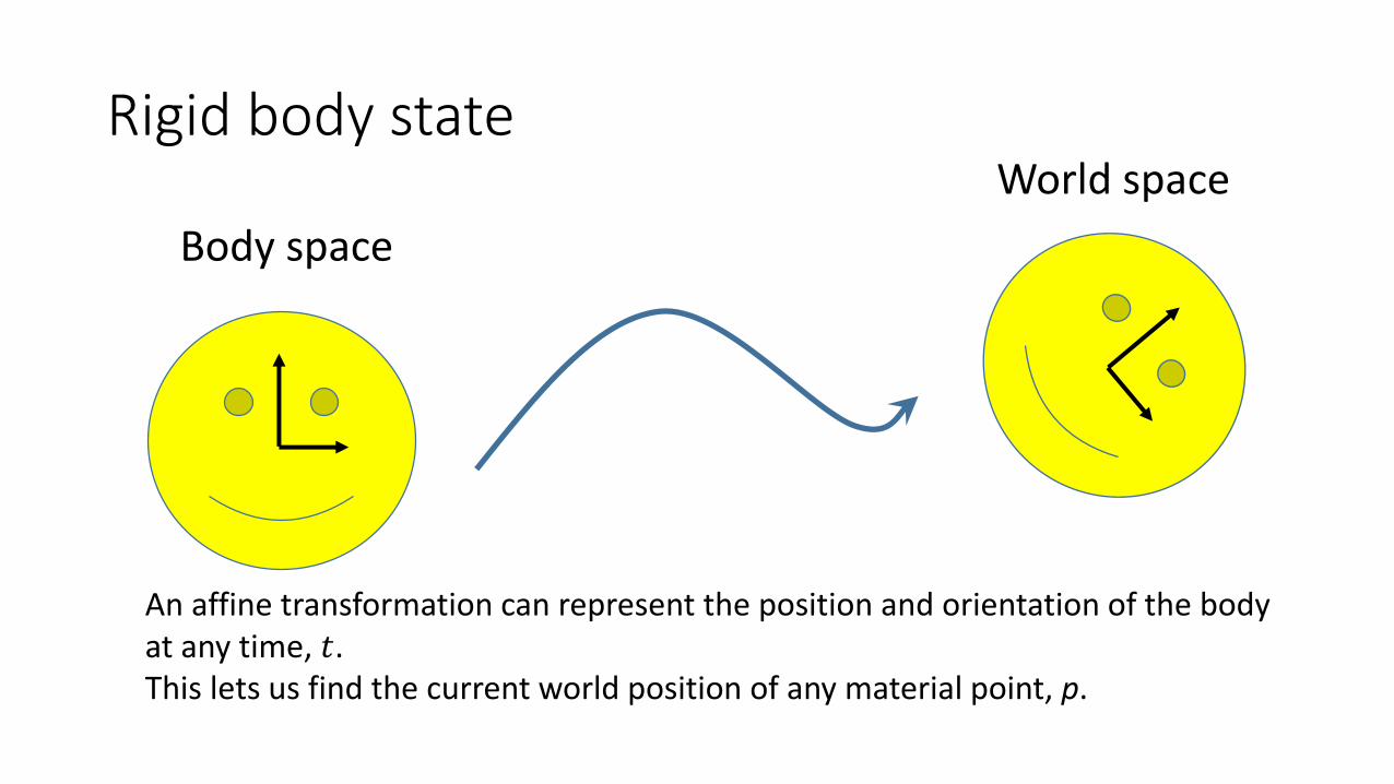
Rigid body state

An affine transformation can represent the position and orientation of the body at any time, 𝑡.This lets us find the current world position of any material point, p.

Body space

World space

Points on the rigid body

If:

• 𝑝0 is the 3D position of a given material point in body space;

• 𝑐(𝑡) is the current 3D position of the centre of mass (in world space);

• 𝑅(𝑡) is the current orientation of the body;

…then the current world position of the point, 𝑝(𝑡) is given by:𝑝 𝑡 = 𝑐 𝑡 + 𝑅 𝑡 𝑝0

Evolving Position – Particle dynamics again!

Treat the centre of mass of the object as a single point/particle, having the full mass of the rigid body.

Solve the usual equations of motion for position and velocity𝑑

𝑑𝑡𝑋𝑉=

𝑉𝐹/𝑀

with your favourite time integration scheme.

How do we evolve the orientation?

Representing Orientation

Choice of representation can be important…

2D: a single angle

3D: • Euler angles (1 angle per axis). (Suffers from “gimbal lock”.)

• 3x3 rotation matrices, R. (We’ll use these for simplicity. 9 numbers for 3 DOFs…)

• Quaternions are also common in practice. (See the Baraff/Witkin notes for more.)

Main question: What are the corresponding equations of motion for orientation? i.e., How does R evolve?

𝑑

𝑑𝑡𝑅?=??

𝑑

𝑑𝑡𝑋𝑉=

𝑉𝐹/𝑀

Position: Orientation:

Angular Velocity

We can represent the rotational speed or angular velocity with a 3D vector, 𝜔(𝑡).

Direction: axis about which we are rotating.

Magnitude: speed at which we are rotating.

𝜔(𝑡)

Rate of change of orientation, 𝑑𝑅

𝑑𝑡

There is a nice relation between angular velocity vector, 𝜔, and rate of change of the orientation/rotation matrix.

𝑑𝑅

𝑑𝑡=

0 −𝜔𝑧 𝜔𝑦𝜔𝑧 0 −𝜔𝑥−𝜔𝑦 𝜔𝑥 0

𝑅

Denote the (skew-symmetric) matrix above by 𝜔∗.

Then we have: 𝑑𝑅

𝑑𝑡= 𝜔∗𝑅

(See Pixar notes for a full derivation, and some intuition.)

So far…

Position update:𝑑𝑋

𝑑𝑡= 𝑉

Analogous orientation update:𝑑𝑅

𝑑𝑡= 𝜔∗𝑅

Next: we need a rotational analog for velocity update, (i.e., 𝑑𝑉

𝑑𝑡=𝐹

𝑚)

Torque

Torque, 𝜏, is the rotational analog of force.

It is computed as:𝜏 = 𝑟 − 𝑐 × 𝐹

for a force F applied at a point 𝑟on the rigid body, where 𝑐 is the centre of mass.

𝑐𝑖(𝑡)𝑟𝑖(𝑡)

𝐹𝑖(𝑡)

Angular momentum

Momentum is a useful conserved quantity (absent forces).

Linear momentum is 𝑃(𝑡) = 𝑚𝑉(𝑡).

Since linear velocity/momentum are proportional, and mass is typically constant, we often just work with linear/translational velocity.

However, angular velocity is not conserved, even in the absence of forces! Trickier to work with.

But angular momentum, 𝐿, is conserved.

Changes in momentum

Momentum does change when there are forces/torques applied.

Linear:

𝑚𝑑𝑉

𝑑𝑡=𝑑𝑃

𝑑𝑡= 𝐹

Angular: 𝑑𝐿

𝑑𝑡= 𝜏

Super! Great!

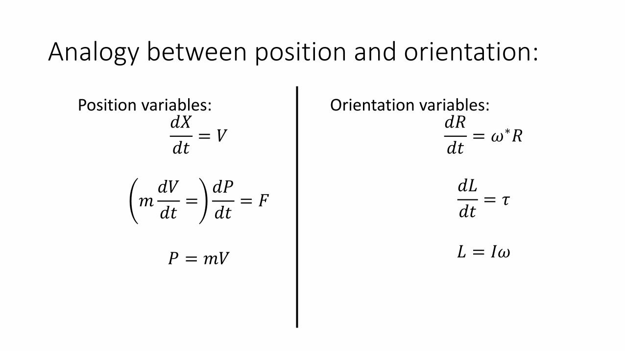
Analogy between position and orientation:

Position variables:𝑑𝑋

𝑑𝑡= 𝑉

𝑚𝑑𝑉

𝑑𝑡=𝑑𝑃

𝑑𝑡= 𝐹

Orientation variables:𝑑𝑅

𝑑𝑡= 𝜔∗𝑅

𝑑𝐿

𝑑𝑡= 𝜏

But how are 𝑅 and 𝐿 related?

Angular Momentum vs. Angular Velocity

The last piece of the puzzle is converting between angular velocity and angular momentum…

𝐿 = 𝐼𝜔

𝐼 is the moment of inertia tensor, a 3x3 matrix that characterizes the distribution of mass relative to the centre of mass point.

Inertia Tensor 𝐼

The rotational counterpart of mass. (Compare 𝐿 = 𝐼𝜔 vs. P = 𝑚𝑉)

Recall: Mass of the rigid body is the integral of density 𝑚 = 𝜌 𝑑𝑉over the object.

Moment of inertia is also an integral:

𝐼 = 𝜌

𝑟𝑦2 + 𝑟𝑧

2 𝑟𝑥𝑟𝑦 𝑟𝑥𝑟𝑧

𝑟𝑥𝑟𝑦 𝑟𝑥2 + 𝑟𝑧

2 𝑟𝑦𝑟𝑧

𝑟𝑥𝑟𝑧 𝑟𝑦𝑟𝑧 𝑟𝑥2 + 𝑟𝑦

2

𝑑𝑉

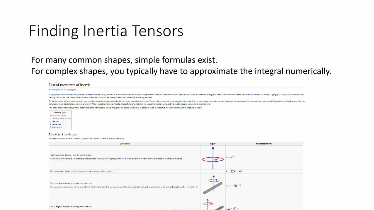
Finding Inertia Tensors

For many common shapes, simple formulas exist.For complex shapes, you typically have to approximate the integral numerically.

Inertia Tensor 𝐼

Subtlety: unlike mass, the current inertia tensor I(t) in world space changes over time!

Re-computing (the integral) for 𝐼(𝑡) at each step could be costly…

Fortunately, it can be shown that:𝐼 𝑡 = 𝑅 𝑡 𝐼𝑏𝑜𝑑𝑦𝑅 𝑡

𝑇

(See Baraff/Witkin’s Pixar notes for a full derivation.)

Rotational Equations of Motion

We now have everything we need to evolve rotation, 𝑑

𝑑𝑡

𝑅?=??:

𝑑

𝑑𝑡𝑅𝐿=𝜔∗𝑅𝜏

Note: At each step we will need to recover the angular velocity 𝜔 from momentum L using:

𝐼 𝑡 = 𝑅 𝑡 𝐼𝑏𝑜𝑑𝑦𝑅 𝑡𝑇 and 𝜔 = 𝐼 𝑡 −1𝐿(𝑡)

Analogy between position and orientation:

Position variables:𝑑𝑋

𝑑𝑡= 𝑉

𝑚𝑑𝑉

𝑑𝑡=𝑑𝑃

𝑑𝑡= 𝐹

𝑃 = 𝑚𝑉

Orientation variables:𝑑𝑅

𝑑𝑡= 𝜔∗𝑅

𝑑𝐿

𝑑𝑡= 𝜏

𝐿 = 𝐼𝜔

Time integration for rigid bodies

Apply your favourite time integration scheme to discretize this full set of equations. (Forward Euler, midpoint, etc.)

Collisions

Two main families.

• Penalty/repulsion methods (briefly, last time)

• Impulse methods (briefly, this time)

Penalty method applies force over some finite period of contact, ∆𝑡.

Impulses are an instantaneous application of force over an infinitesimal period, i.e., conceptual limit as ∆𝑡 → 0.

Impulses – Elastic Collisions

Consider an ideal rubber ball falling onto a flat plane. How must the (vertical) velocity change for the ball to bounce perfectly?

𝑉𝑦 = −1 𝑉𝑦 = +1

We just reflect the (normal component of) velocity.

Impulses – Inelastic Collisions

Consider a heavy stone falling onto a flat plane. Nearly all of the energy is dissipated in the collision.

𝑉𝑦 = −1 𝑉𝑦 = 0

We entirely eliminate the(normal component of) velocity.

Coefficient of Restitution

Most collisions are somewhere between.

Coefficient of restitution, 𝜖 ∈ [0,1], models the fraction of energy remaining after a collision. Putting it together…

𝑉𝑟𝑒𝑙,𝑛𝑎𝑓𝑡𝑒𝑟

= −𝜖𝑉𝑟𝑒𝑙,𝑛𝑏𝑒𝑓𝑜𝑟𝑒

Note! Only the (relative) velocity in the normal direction changes.Tangential velocity is left alone (until you add friction…)

See: e.g. “Nonconvex Rigid Bodies with Stacking” [Guendelman 2003] for a summary of the general case, with friction and rotational collision impulses.

Some Interesting Recent Examples

• Drawn from [Kaufman et al. 2008] and [Smith et al. 2012], on our papers list.

Physics-Based Animation

If you’re interested in following along with recent/new research papers, check out:

www.physicsbasedanimation.com