Lecture 13 Time Series: Stationarity, AR(p) & MA(q) · Lecture 13 Time Series: Stationarity, AR(p) ... ergodic theorem will give us a counterpart to the LLN. ... Difficult to prove

RS – EC2 - Lecture 13

1

1

Lecture 13Time Series:

Stationarity, AR(p) & MA(q)

Time Series: Introduction

• In the early 1970’s, it was discovered that simple time series models performed better than the complicated multivarate, then popular, 1960s macro models (FRB-MIT-Penn). See, Nelson (1972).

• The tools? Simple univariate (ARIMA) models, popularized by the textbook of Box & Jenkins (1970).

Q: What is a time series? A time series yt is a process observed in sequence over time, t = 1,...., T => Yt={y1, y2 , y3, ..., yT}

• Because of the sequential nature of Yt, we expect that yt and yt-1 to be dependent. Then, classical assumptions are not valid.


2

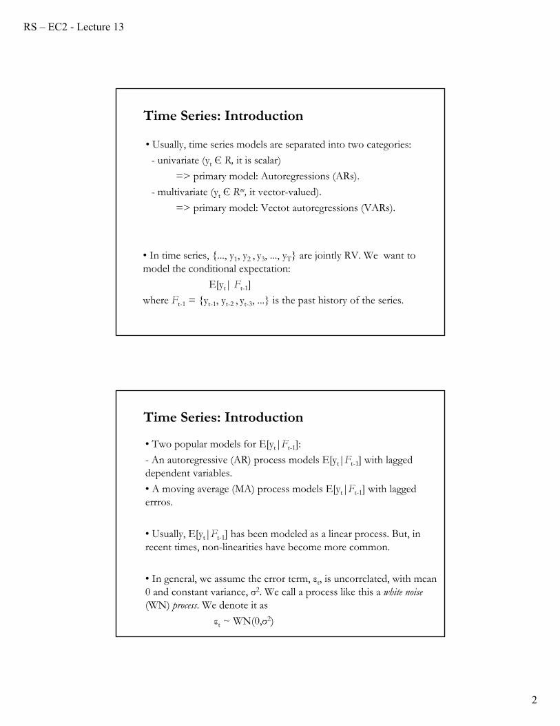
• Usually, time series models are separated into two categories:

- univariate (yt Є R, it is scalar)

=> primary model: Autoregressions (ARs).

- multivariate (yt Є Rm, it vector-valued).

=> primary model: Vectot autoregressions (VARs).

• In time series, {..., y1, y2 , y3, ..., yT} are jointly RV. We want to model the conditional expectation:

E[yt| Ft-1]

where Ft-1 = {yt-1, yt-2 , yt-3, ...} is the past history of the series.


• Two popular models for E[yt|Ft-1]:

- An autoregressive (AR) process models E[yt|Ft-1] with lagged dependent variables.

• A moving average (MA) process models E[yt|Ft-1] with lagged errros.

• Usually, E[yt|Ft-1] has been modeled as a linear process. But, in recent times, non-linearities have become more common.

• In general, we assume the error term, εt, is uncorrelated, with mean 0 and constant variance, σ2. We call a process like this a white noise (WN) process. We denote it as

εt ~ WN(0,σ2)



3

CLM Revisited: Time Series

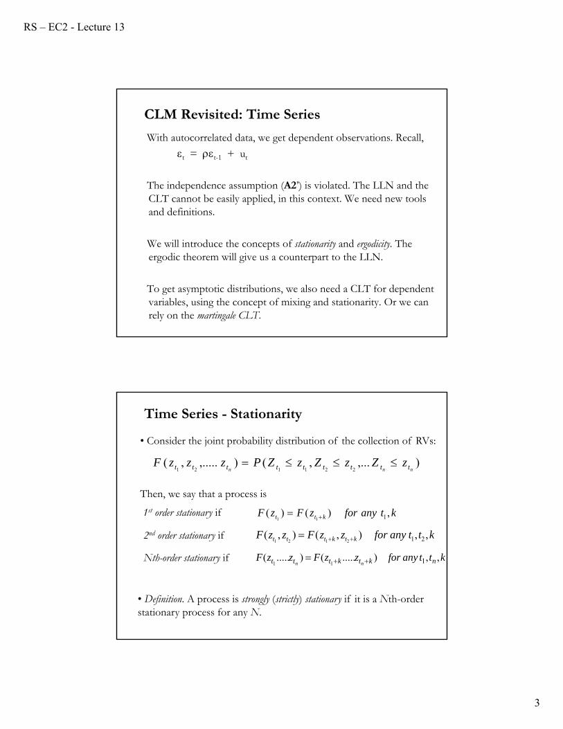
With autocorrelated data, we get dependent observations. Recall,

t = t-1 + ut

The independence assumption (A2’) is violated. The LLN and the CLT cannot be easily applied, in this context. We need new tools and definitions.

We will introduce the concepts of stationarity and ergodicity. The ergodic theorem will give us a counterpart to the LLN.

To get asymptotic distributions, we also need a CLT for dependent variables, using the concept of mixing and stationarity. Or we can rely on the martingale CLT.

• Consider the joint probability distribution of the collection of RVs:

Then, we say that a process is

),...,(),.....,(221121 nnn ttttttttt zZzZzZPzzzF

1st order stationary if ktanyforzFzF ktt ,)()( 111

Nth-order stationary if

kttanyforzzFzzF ktkttt ,,),(),( 212121

kttanyforzzFzzF nktkttt nn,,).....().....( 111

• Definition. A process is strongly (strictly) stationary if it is a Nth-order stationary process for any N.

2nd order stationary if

Time Series - Stationarity


4

22

2121

21

222

21

221121

)(),(

)()])([(),(

)()()()(

)()(

tt

tttttt

tttttttt

ttttt

tttt

ttZZEZZCov

dzzfZZEZVar

dzzfZZE

Time Series – Moments

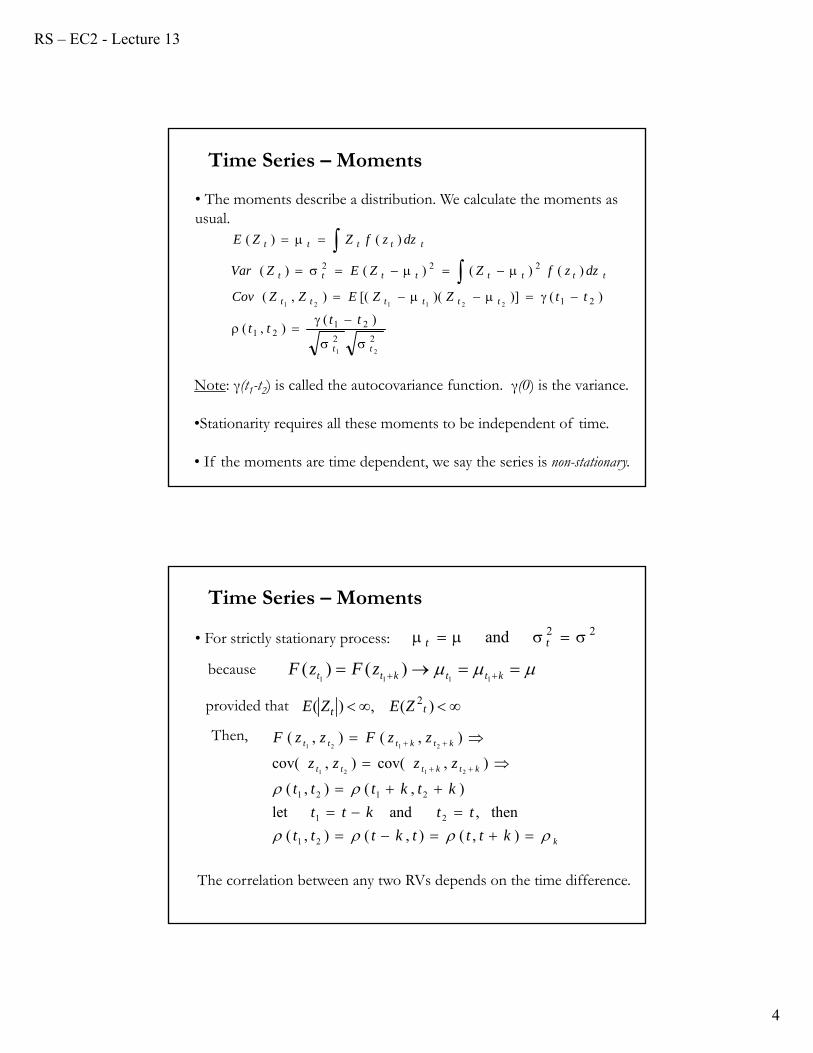
• The moments describe a distribution. We calculate the moments as usual.

Note: γ(t1-t2) is called the autocovariance function. γ(0) is the variance.

•Stationarity requires all these moments to be independent of time.

• If the moments are time dependent, we say the series is non-stationary.

• For strictly stationary process: 22and tt

because kttktt zFzF1111

)()(

provided that

k

ktkttt

ktkttt

ktttkttt

ttktt

ktkttt

zzzz

zzFzzF

),(),(),(

then, and let

),(),(

),cov(),cov(

),(),(

21

21

2121

2121

2121

The correlation between any two RVs depends on the time difference.

)(,)( 2tt ZEZE

Then,

Time Series – Moments


5

• A process is said to be N-order weakly stationary if all its joint moments up to order N exist and are time invariant.

• A Covariance stationary process (or 2nd order weakly stationary) has:- constant mean- constant variance- covariance function depends on time difference between R.V.

That is, Zt is covariance stationary if:

Time Series – Weak Stationarity

)()()])([(),(

constant)(

constant)(

2121221121ttfttZZEZZCov

ZVar

ZE

tttttt

t

t

Examples: For all assume εt ~ WN(0,σ2)

1) yt = Φ yt-1 + εt

E[yt ] = 0 (assuming Φ≠1)Var[yt] = σ2/(1-Φ2) (assuming |Φ|<11)E[yt yt-1] = Φ E[yt-1

2]=> stationary, not time dependent

2) yt = μ + yt-1 + εt =>yt = μ t + Σj=0 to t-1 εt-j + y0

E[yt ] = μ t + y0

Var[yt] = Σj=0 to t-1 σ2 = σ2 t=> non-stationary, time dependent

Time Series – Weak Stationarity


6

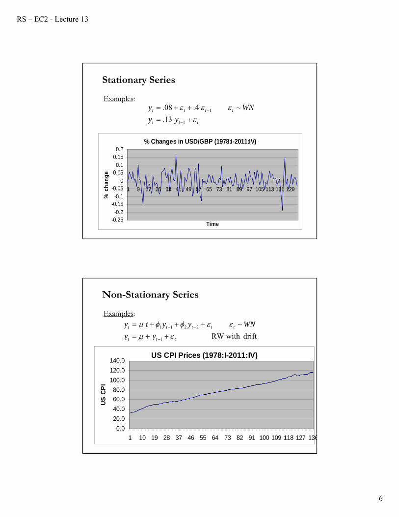
Stationary Series

13.

~4.08.

1

1

ttt

tttt

yy

WNy

Examples:

% Changes in USD/GBP (1978:I-2011:IV)

-0.25-0.2

-0.15-0.1

-0.050

0.050.1

0.150.2

1 9 17 25 33 41 49 57 65 73 81 89 97 105 113 121 129

Time

% c

han

ge

Non-Stationary Series

Examples:

driftRW with

~

1

2211

ttt

ttttt

yy

WNyyty

US CPI Prices (1978:I-2011:IV)

0.0

20.0

40.0

60.0

80.0

100.0

120.0

140.0

1 10 19 28 37 46 55 64 73 82 91 100 109 118 127 136

US

CP

I


7

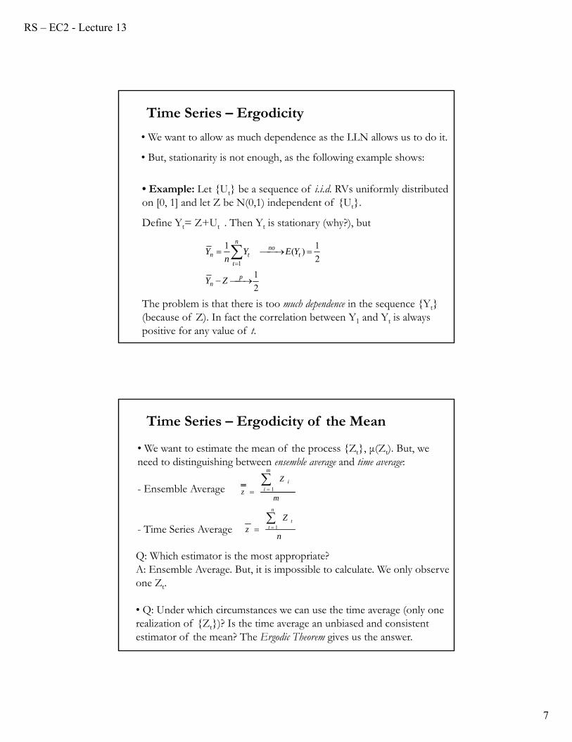
• We want to allow as much dependence as the LLN allows us to do it.

• But, stationarity is not enough, as the following example shows:

• Example: Let {Ut} be a sequence of i.i.d. RVs uniformly distributed on [0, 1] and let Z be N(0,1) independent of {Ut}.

Define Yt= Z+Ut . Then Yt is stationary (why?), but

The problem is that there is too much dependence in the sequence {Yt} (because of Z). In fact the correlation between Y1 and Yt is always positive for any value of t.

2

1

2

1)(

1

1

pn

tno

n

ttn

ZY

YEYn

Y

Time Series – Ergodicity

• We want to estimate the mean of the process {Zt}, μ(Zt). But, we need to distinguishing between ensemble average and time average:

- Ensemble Average

- Time Series Average

Q: Which estimator is the most appropriate? A: Ensemble Average. But, it is impossible to calculate. We only observe one Zt.

• Q: Under which circumstances we can use the time average (only one realization of {Zt})? Is the time average an unbiased and consistent estimator of the mean? The Ergodic Theorem gives us the answer.

m

Z

z

m

ii

1

n

Zz

n

tt

1

Time Series – Ergodicity of the Mean


8

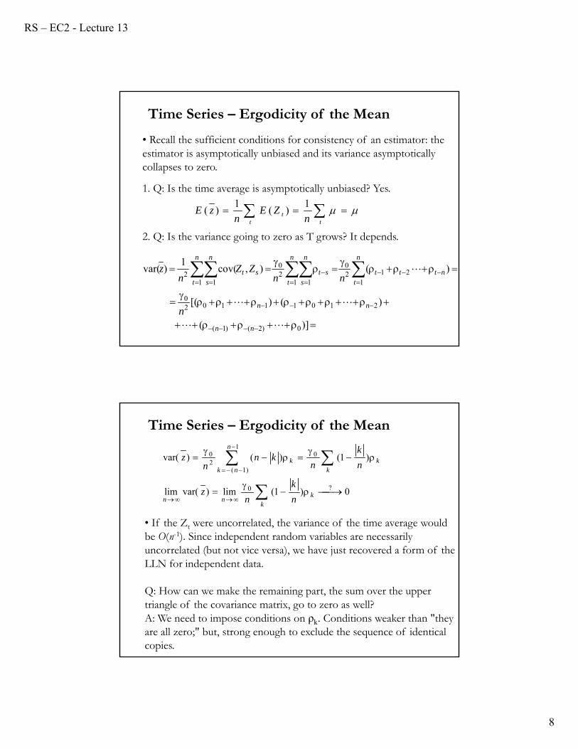
• Recall the sufficient conditions for consistency of an estimator: the estimator is asymptotically unbiased and its variance asymptotically collapses to zero.

1. Q: Is the time average is asymptotically unbiased? Yes.

t t

t nZE

nzE 1

)(1

)(

2. Q: Is the variance going to zero as T grows? It depends.

)](

)()[(

)(),cov(1

)var(

0)2()1(

210111020

1212

0

1 120

1 12

nn

nn

n

tnttt

n

t

n

sst

n

t

n

sst

n

nnZZ

nz


0)1(lim)var(lim

)1()()var(

?0

1

)1(

020

kk

nn

n

nk kkk

n

k

nz

n

k

nkn

nz

• If the Zt were uncorrelated, the variance of the time average would be O(n-1). Since independent random variables are necessarily uncorrelated (but not vice versa), we have just recovered a form of the LLN for independent data.

Q: How can we make the remaining part, the sum over the upper triangle of the covariance matrix, go to zero as well? A: We need to impose conditions on ρk. Conditions weaker than "they are all zero;" but, strong enough to exclude the sequence of identical copies.



9

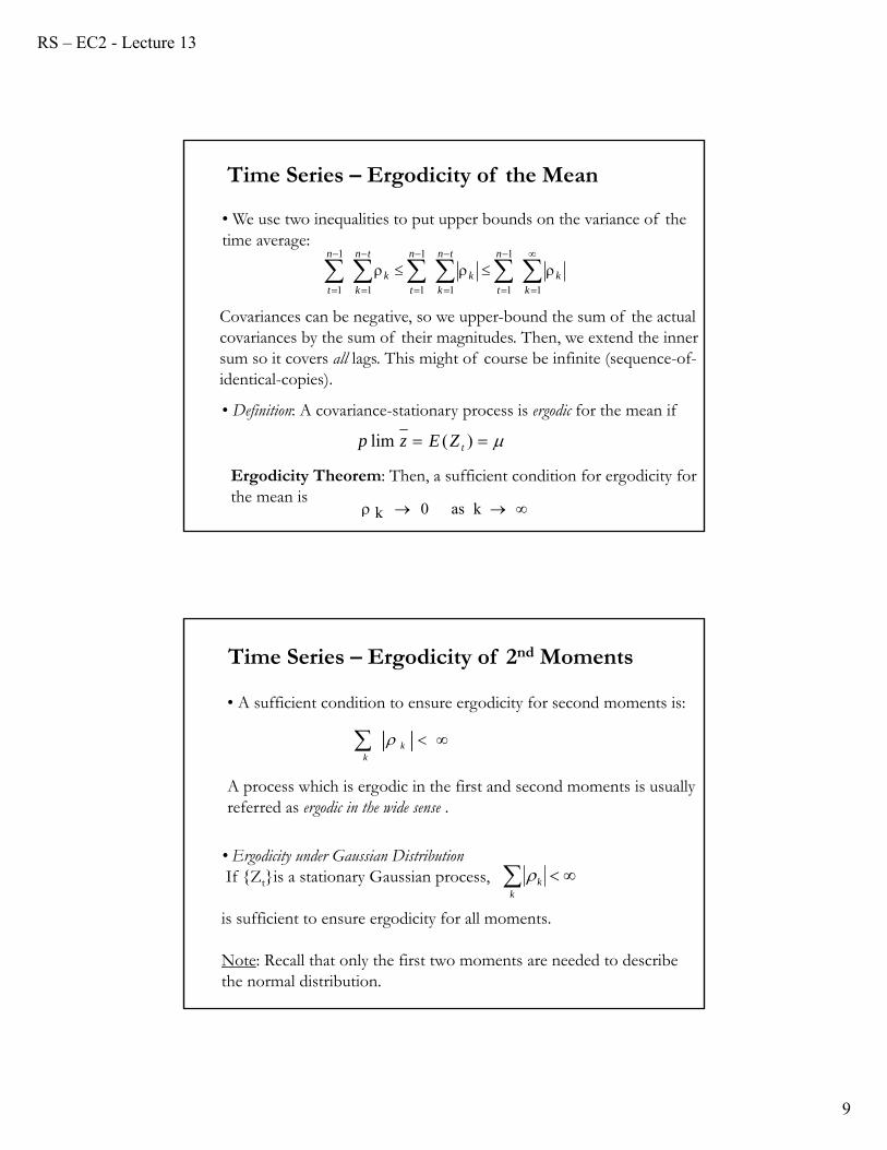
• Definition: A covariance-stationary process is ergodic for the mean if

)(lim tZEzp

Ergodicity Theorem: Then, a sufficient condition for ergodicity for the mean is

k as 0k

1

1

11

1

11

1

1 kk

n

t

tn

kk

n

t

tn

kk

n

t

• We use two inequalities to put upper bounds on the variance of the time average:

Covariances can be negative, so we upper-bound the sum of the actual covariances by the sum of their magnitudes. Then, we extend the inner sum so it covers all lags. This might of course be infinite (sequence-of-identical-copies).


• Ergodicity under Gaussian DistributionIf {Zt}is a stationary Gaussian process,

is sufficient to ensure ergodicity for all moments.

Note: Recall that only the first two moments are needed to describe the normal distribution.

k

k

• A sufficient condition to ensure ergodicity for second moments is:

A process which is ergodic in the first and second moments is usually referred as ergodic in the wide sense .

k

k

Time Series – Ergodicity of 2nd Moments


10

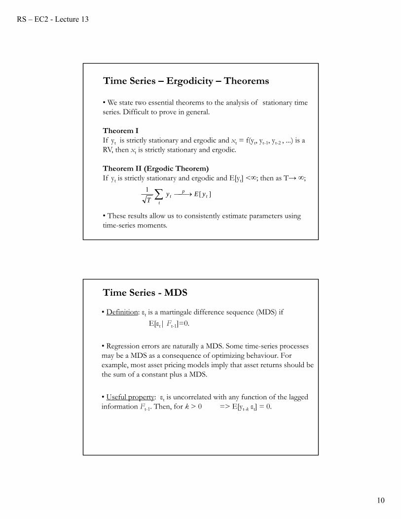
• We state two essential theorems to the analysis of stationary time series. Difficult to prove in general.

Theorem IIf yt is strictly stationary and ergodic and xt = f(yt, yt-1, yt-2 , ...) is a RV, then xt is strictly stationary and ergodic.

Theorem II (Ergodic Theorem)If yt is strictly stationary and ergodic and E[yt] <∞; then as T→ ∞;

• These results allow us to consistently estimate parameters using time-series moments.

Time Series – Ergodicity – Theorems

][1

tp

tt yEy

T

• Definition: εt is a martingale difference sequence (MDS) if

E[εt| Ft-1]=0.

• Regression errors are naturally a MDS. Some time-series processes may be a MDS as a consequence of optimizing behaviour. For example, most asset pricing models imply that asset returns should be the sum of a constant plus a MDS.

• Useful property: εt is uncorrelated with any function of the lagged information Ft-1. Then, for k > 0 => E[yt-k εt] = 0.

Time Series - MDS


11

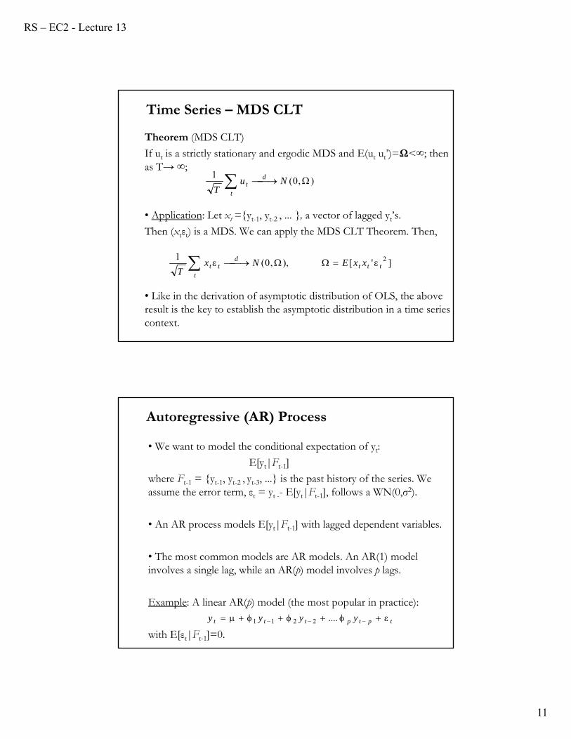
Theorem (MDS CLT)

If ut is a strictly stationary and ergodic MDS and E(ut ut’)=Ω<∞; then as T→ ∞;

• Application: Let xt ={yt-1, yt-2 , ... }, a vector of lagged yt’s.

Then (xtεt) is a MDS. We can apply the MDS CLT Theorem. Then,

• Like in the derivation of asymptotic distribution of OLS, the above result is the key to establish the asymptotic distribution in a time series context.

Time Series – MDS CLT

),0(1

NuT

d

tt

]'[),,0(1 2

tttd

ttt xxENx

T

Autoregressive (AR) Process

• We want to model the conditional expectation of yt:

E[yt|Ft-1]

where Ft-1 = {yt-1, yt-2 , yt-3, ...} is the past history of the series. We assume the error term, εt = yt -- E[yt|Ft-1], follows a WN(0,σ2).

• An AR process models E[yt|Ft-1] with lagged dependent variables.

• The most common models are AR models. An AR(1) model involves a single lag, while an AR(p) model involves p lags.

Example: A linear AR(p) model (the most popular in practice):

with E[εt|Ft-1]=0.tptpttt yyyy ....2211


12

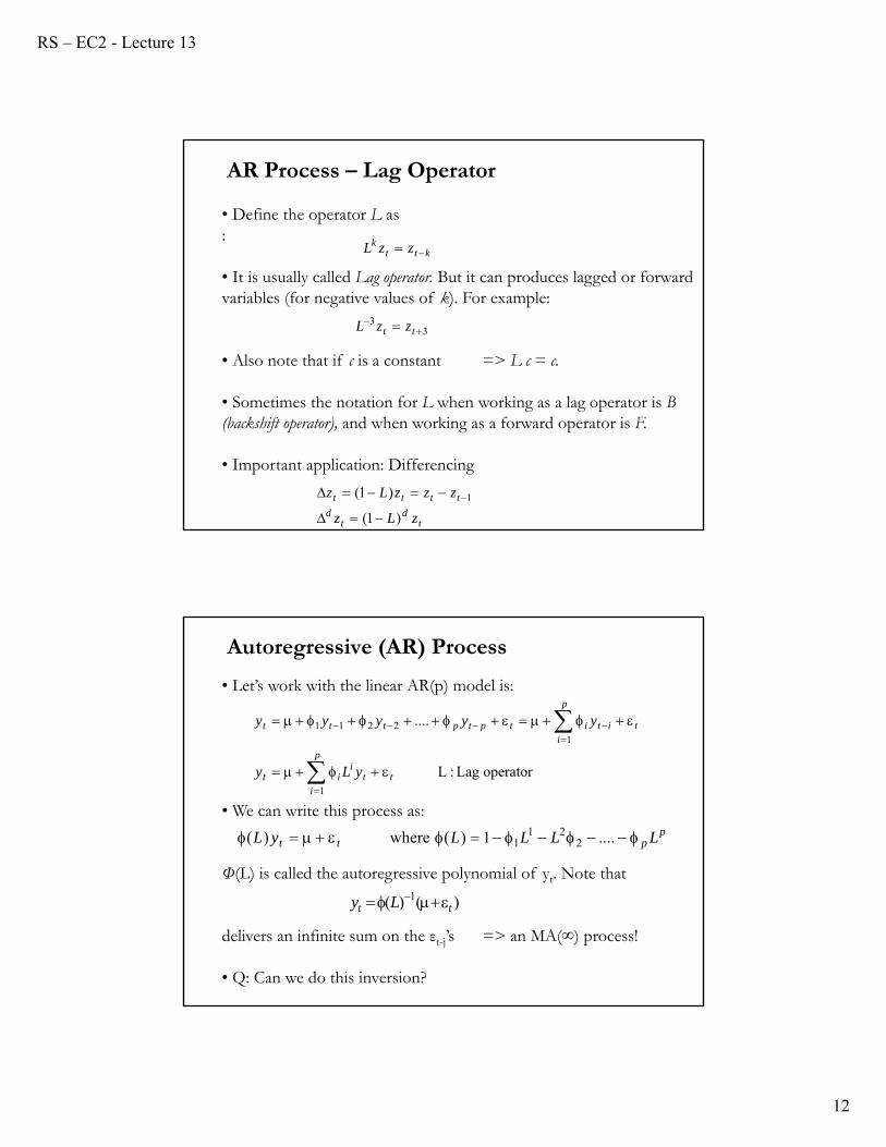
• Define the operator L as:

• It is usually called Lag operator. But it can produces lagged or forward variables (for negative values of k). For example:

• Also note that if c is a constant => L c = c.

• Sometimes the notation for L when working as a lag operator is B (backshift operator), and when working as a forward operator is F.

• Important application: Differencing

kttk zzL

AR Process – Lag Operator

33

tt zzL

td

td

tttt

zLz

zzzLz

)1(

)1( 1

• Let’s work with the linear AR(p) model is:

• We can write this process as:

Φ(L) is called the autoregressive polynomial of yt. Note that

delivers an infinite sum on the εt-j’s => an MA(∞) process!

• Q: Can we do this inversion?

)()( 1tt Ly

pptt LLLLyL ....1)( where )( 2

211

operator Lag :L

....

1

12211

tti

p

iit

tit

p

iitptpttt

yLy

yyyyy

Autoregressive (AR) Process


13

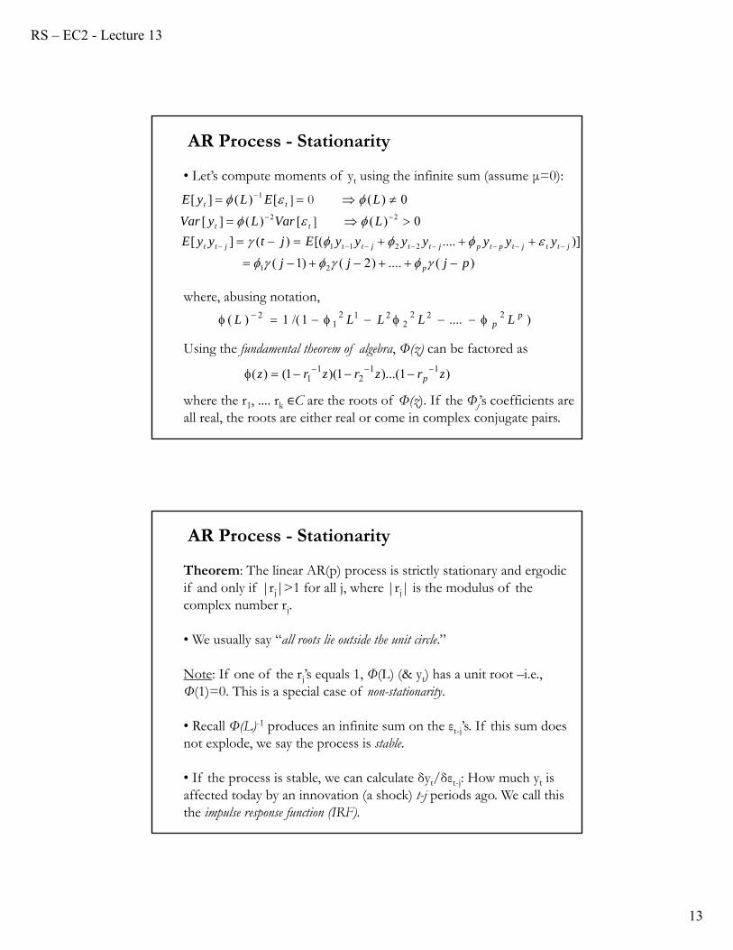
• Let’s compute moments of yt using the infinite sum (assume μ=0):

where, abusing notation,

Using the fundamental theorem of algebra, Φ(z) can be factored as

where the r1, .... rk ∈C are the roots of Φ(z). If the Φj’s coefficients are all real, the roots are either real or come in complex conjugate pairs.

AR Process - Stationarity

)(....)2()1(

)]....[()(][

0)([)(][

0)([)(][

21

2211

22

1

pjjj

yyyyyyyEjtyyE

LVarLyVar

LELyE

p

jttjtptpjttjttjtt

tt

tt

]

0]

)1)...(1)(1()( 112

11 zrzrzrz p

)....1/(1)( 2222

2121

2 pp LLLLL

Theorem: The linear AR(p) process is strictly stationary and ergodic if and only if |rj|>1 for all j, where |rj| is the modulus of the complex number rj.

• We usually say “all roots lie outside the unit circle.”

Note: If one of the rj’s equals 1, Φ(L) (& yt) has a unit root –i.e., Φ(1)=0. This is a special case of non-stationarity.

• Recall Φ(L)-1 produces an infinite sum on the εt-j’s. If this sum does not explode, we say the process is stable.

• If the process is stable, we can calculate δyt/δεt-j: How much yt is affected today by an innovation (a shock) t-j periods ago. We call this the impulse response function (IRF).



14

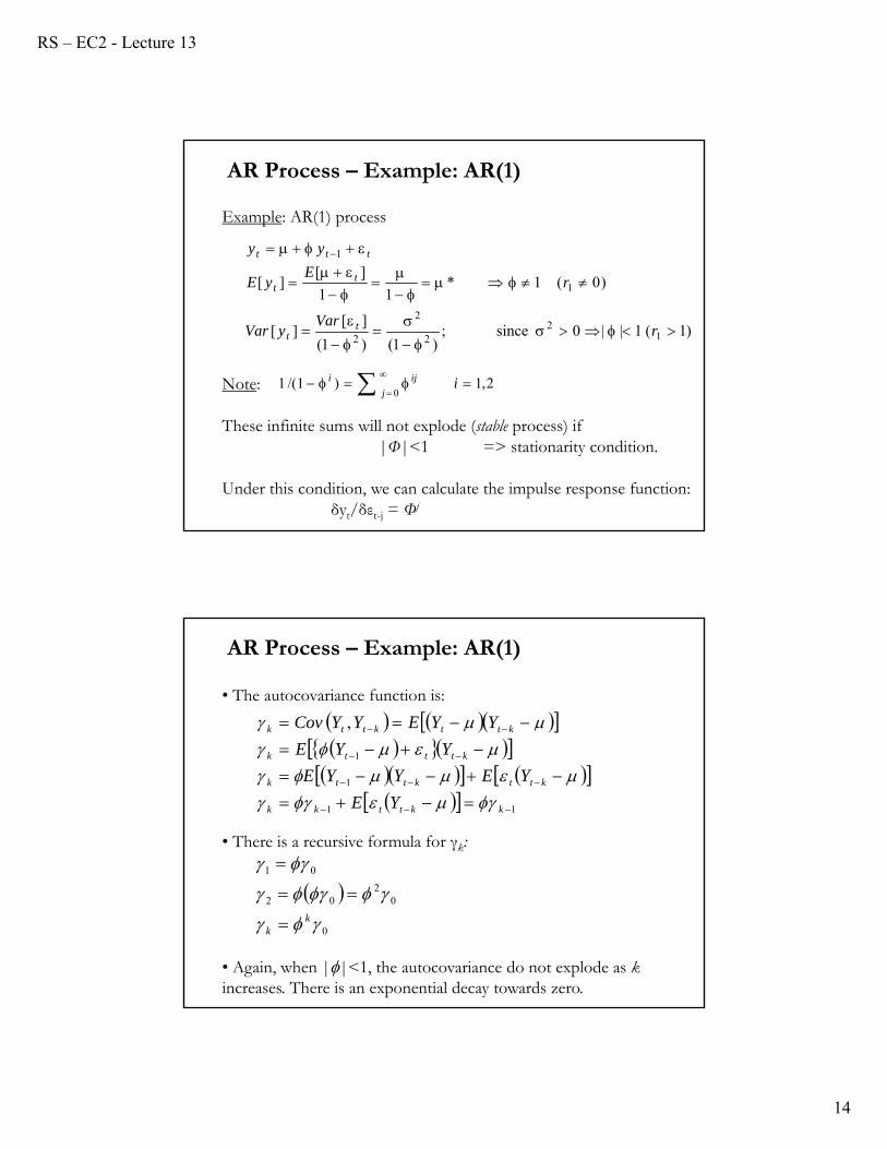
Example: AR(1) process

Note:

These infinite sums will not explode (stable process) if |Φ|<1 => stationarity condition.

Under this condition, we can calculate the impulse response function:δyt/δεt-j = Φj

AR Process – Example: AR(1)

)1(1||0since;)1()1(

][][

)0(1*11

][][

12

2

2

2

1

1

rVar

yVar

rE

yE

yy

tt

tt

ttt

2,1)1/(10

i

j

iji

• The autocovariance function is:

• There is a recursive formula for γk:

• Again, when ||<1, the autocovariance do not explode as k increases. There is an exponential decay towards zero.


11

1

1

,

kkttkk

kttkttk

ktttk

kttkttk

YE

YEYYE

YYE

YYEYYCov

0

02

02

01

kk


15

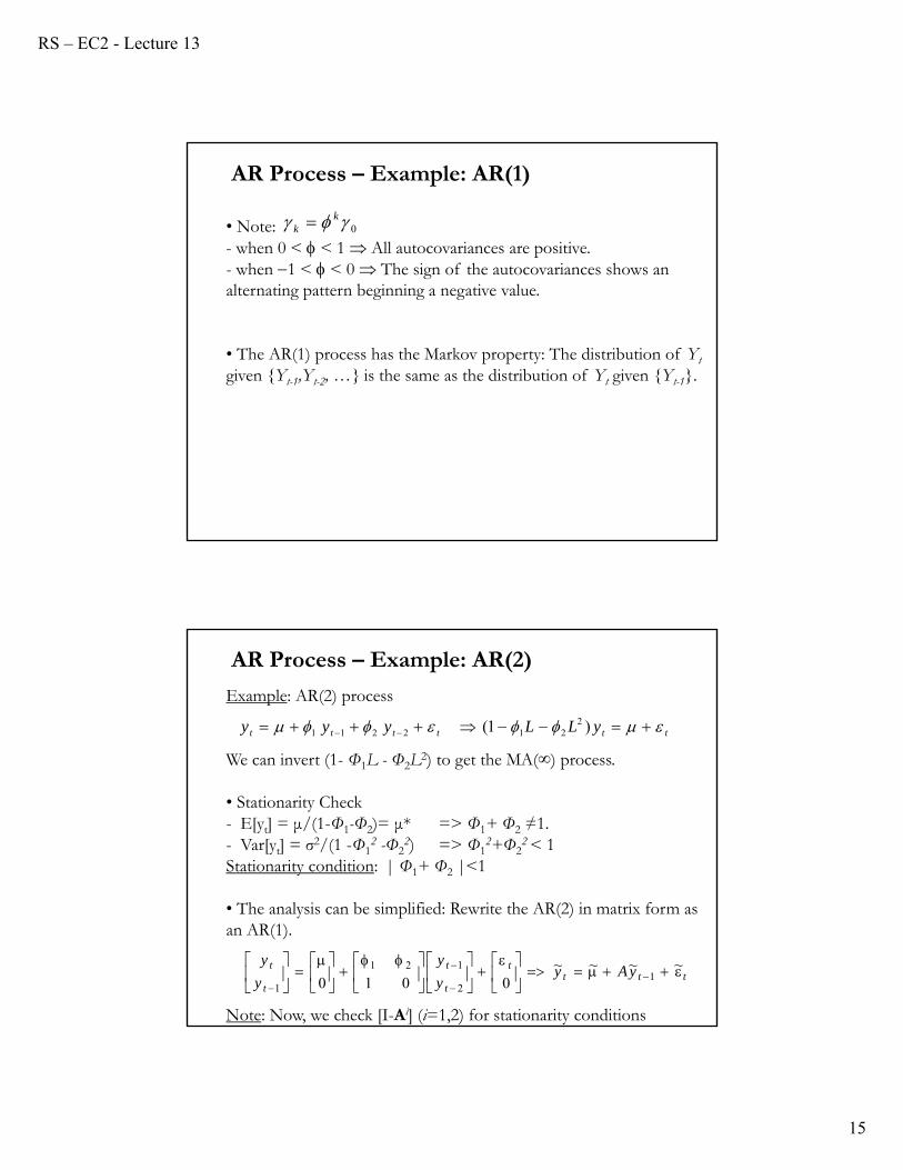
• Note:- when 0 < < 1 All autocovariances are positive.- when 1 < < 0 The sign of the autocovariances shows an alternating pattern beginning a negative value.

• The AR(1) process has the Markov property: The distribution of Yt

given {Yt-1,Yt-2, …} is the same as the distribution of Yt given {Yt-1}.


0 kk

Example: AR(2) process

We can invert (1- Φ1L - Φ2L2) to get the MA(∞) process.

• Stationarity Check- E[yt] = μ/(1-Φ1-Φ2)= μ* => Φ1+ Φ2 ≠1.- Var[yt] = σ2/(1 -Φ1

2 -Φ22) => Φ1

2+Φ22 < 1

Stationarity condition: | Φ1+ Φ2 |<1

• The analysis can be simplified: Rewrite the AR(2) in matrix form as an AR(1).

Note: Now, we check [I-Ai] (i=1,2) for stationarity conditions


tttttt yLLyyy )1( 2212211

tttt

t

t

t

t yAyy

y

y

y

~~~~0010 1

2

121

1


16

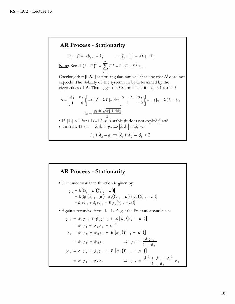
Note: Recall

Checking that [I-AL] is not singular, same as checking that Aj does not explode. The stability of the system can be determined by the eigenvalues of A. That is, get the λi’s and check if |λi| <1 for all i.

• If |λi| <1 for all i=1,2, yt is stable (it does not explode) and stationary. Then:


212121 )(

1det||

01

IAA

.2

0

1 ..FFIFFIj

j

ttttt ALIyyAy

~][~~~~~ 11

2

1

121121

221221

• The autocovariance function is given by:

• Again a recursive formula. Let’s get the first autocovariances:


kttkk

ktttt

kttk

YE

YYYE

YYE

2211

2211

02

222

21

22211

222112

2

0111201

112011

22211

22110

1

1

tt

tt

tt

YE

YE

YE


17

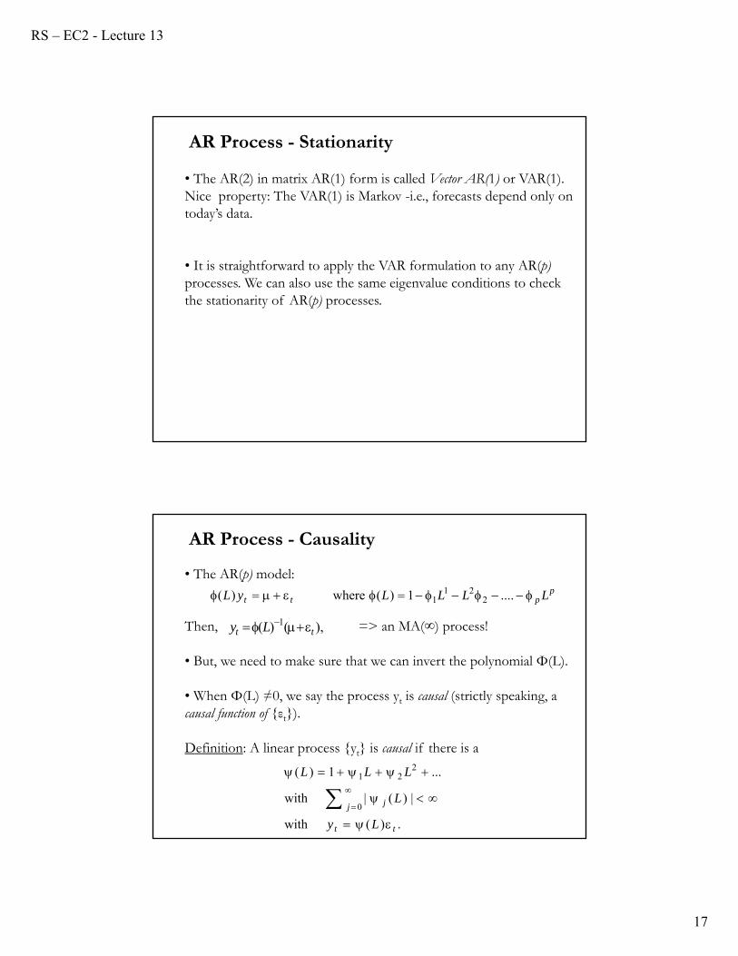
• The AR(2) in matrix AR(1) form is called Vector AR(1) or VAR(1). Nice property: The VAR(1) is Markov -i.e., forecasts depend only on today’s data.

• It is straightforward to apply the VAR formulation to any AR(p) processes. We can also use the same eigenvalue conditions to check the stationarity of AR(p) processes.


• The AR(p) model:

Then, => an MA(∞) process!

• But, we need to make sure that we can invert the polynomial Φ(L).

• When Φ(L) ≠0, we say the process yt is causal (strictly speaking, a causal function of {εt}).

Definition: A linear process {yt} is causal if there is a

AR Process - Causality

.)(with

|)(|with

...1)(

0

221

tt

j j

Ly

L

LLL

pptt LLLLyL ....1)( where )( 2

211

),()( 1tt Ly


18

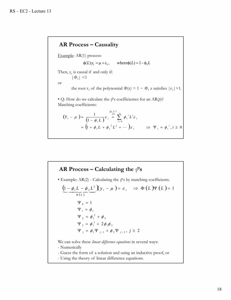
Example: AR(1) process:

Then, yt is causal if and only if: |Φ1| <1

orthe root r1 of the polynomial Φ(z) = 1 − Φ1 z satisfies |r1|>1.

• Q: How do we calculate the ψ‘s coefficientes for an AR(p)? Matching coefficients:

AR Process – Causality

LLyL tt 11)( where ,)(

0,1

1

1

122

11

01

1

1

1

iLL

LL

Y

iit

it

iitt

• Example: AR(2) - Calculating the ψ‘s by matching coefficients.

AR Process – Calculating the ψ’s

We can solve these linear difference equations in several ways:- Numerically- Guess the form of a solution and using an inductive proof, or- Using the theory of linear difference equations.

2,

2

1

2211

213

13

22

12

11

0

jjjj

11 221

LLyLL tt

L


19

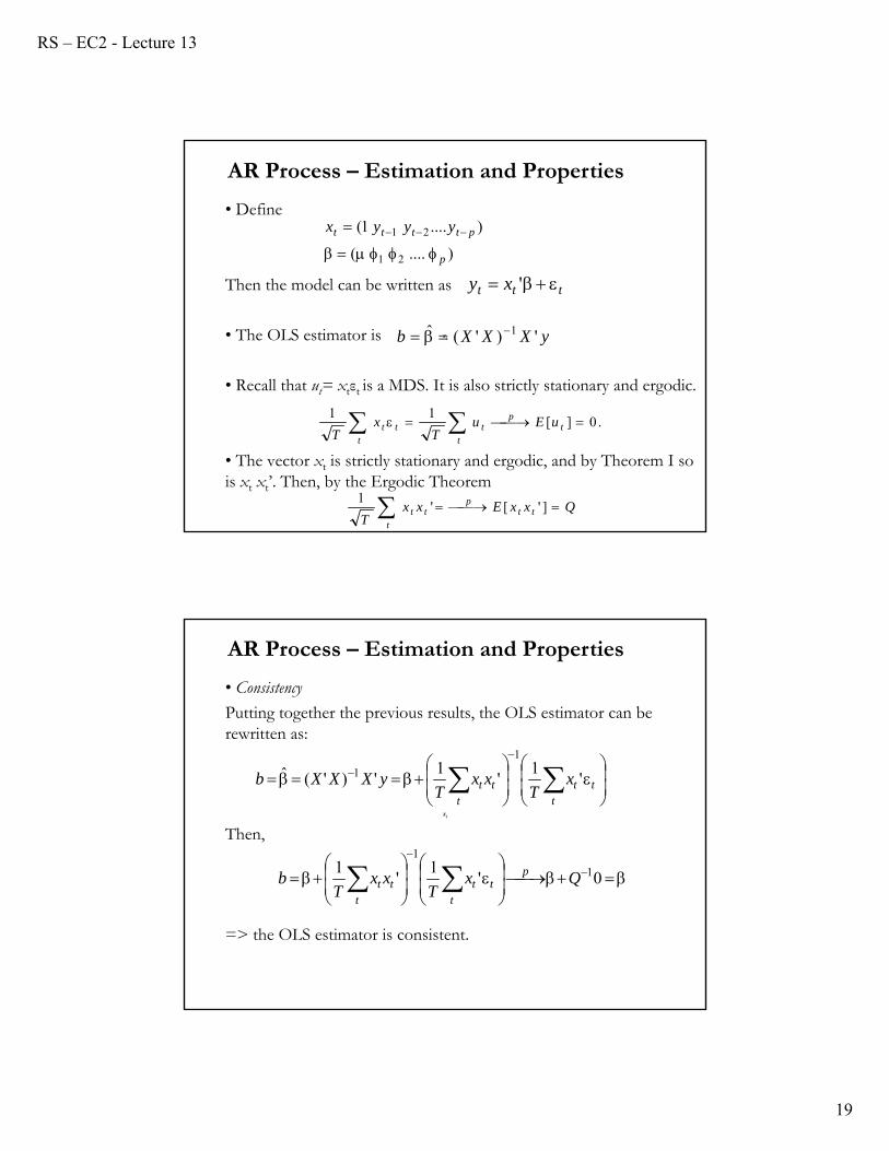
• Define

Then the model can be written as

• The OLS estimator is

• Recall that ut= xtεt is a MDS. It is also strictly stationary and ergodic.

• The vector xt is strictly stationary and ergodic, and by Theorem I so is xt xt’. Then, by the Ergodic Theorem

AR Process – Estimation and Properties

)....(

)....1(

21

21

p

ptttt yyyx

ttt xy '

tx yXXXb ')'(ˆ 1

.0][11

tp

t tttt uEu

Tx

T

QxxExxT

ttp

ttt ]'['

1

• Consistency

Putting together the previous results, the OLS estimator can be rewritten as:

Then,

=> the OLS estimator is consistent.

AR Process – Estimation and Properties

tx

ttt

ttt x

Txx

TyXXXb '

1'

1')'(ˆ

1

1

0'1

'1 1

1

QxT

xxT

b p

ttt

ttt


20

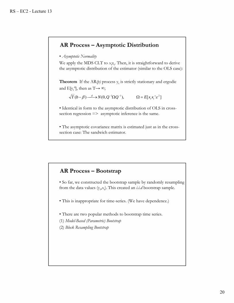
• Asymptotic Normality

We apply the MDS CLT to xtεt. Then, it is straightforward to derive the asymptotic distribution of the estimator (similar to the OLS case):

Theorem If the AR(p) process yt is strictly stationary and ergodic

and E[yt4], then as T→ ∞;

• Identical in form to the asymptotic distribution of OLS in cross-section regression => asymptotic inference is the same.

• The asymptotic covariance matrix is estimated just as in the cross-section case: The sandwich estimator.

AR Process – Asymptotic Distribution

]'[),,0()( 211 ttd xxEQQNbT

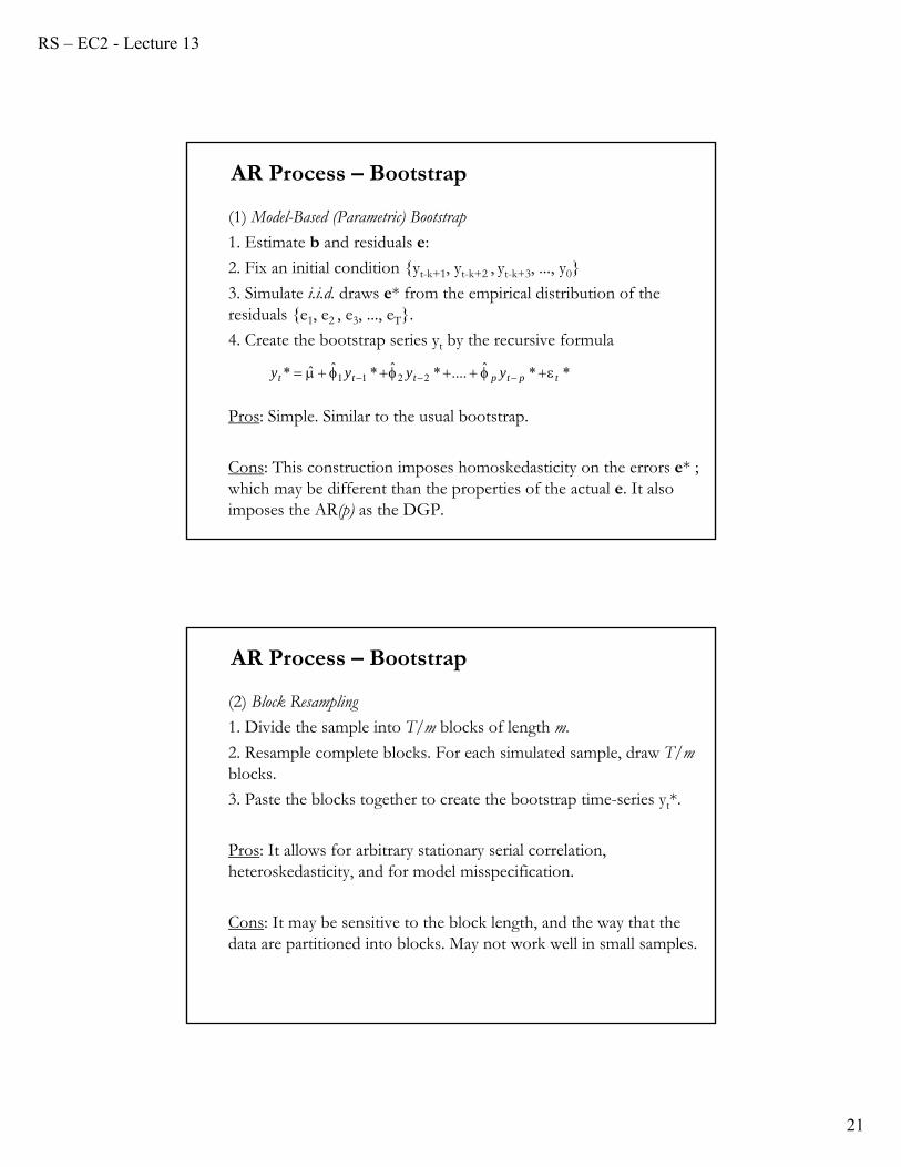
• So far, we constructed the bootstrap sample by randomly resampling from the data values (yt,xt). This created an i.i.d bootstrap sample.

• This is inappropriate for time-series. (We have dependence.)

• There are two popular methods to bootstrap time series.

(1) Model-Based (Parametric) Bootstrap

(2) Block Resampling Bootstrap

AR Process – Bootstrap


21

(1) Model-Based (Parametric) Bootstrap

1. Estimate b and residuals e:

2. Fix an initial condition {yt-k+1, yt-k+2 , yt-k+3, ..., y0}

3. Simulate i.i.d. draws e* from the empirical distribution of the residuals {e1, e2 , e3, ..., eT}.

4. Create the bootstrap series yt by the recursive formula

Pros: Simple. Similar to the usual bootstrap.

Cons: This construction imposes homoskedasticity on the errors e* ; which may be different than the properties of the actual e. It also imposes the AR(p) as the DGP.


**ˆ....*ˆ*ˆˆ* 2211 tptpttt yyyy

(2) Block Resampling

1. Divide the sample into T/m blocks of length m.

2. Resample complete blocks. For each simulated sample, draw T/mblocks.

3. Paste the blocks together to create the bootstrap time-series yt*.

Pros: It allows for arbitrary stationary serial correlation, heteroskedasticity, and for model misspecification.

Cons: It may be sensitive to the block length, and the way that the data are partitioned into blocks. May not work well in small samples.



22

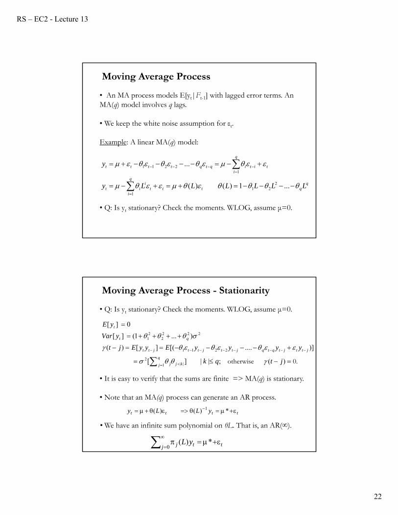
• An MA process models E[yt|Ft-1] with lagged error terms. An MA(q) model involves q lags.

• We keep the white noise assumption for εt.

Example: A linear MA(q) model:

• Q: Is yt stationary? Check the moments. WLOG, assume μ=0.

Moving Average Process

qqtt

q

it

iit

tit

q

iiqtqtttt

LLLLLLy

y

...1)()(

...

221

1

12211

• Q: Is yt stationary? Check the moments. WLOG, assume μ=0.

• It is easy to verify that the sums are finite => MA(q) is stationary.

• Note that an MA(q) process can generate an AR process.

• We have an infinite sum polynomial on θL. That is, an AR(∞).

Moving Average Process - Stationarity

0. otherwise

)(;||][

)]....[(][)(

)...1(][

0][

1 ||2

2211

2222

21

jtqk

yyyyEyyEjt

yVar

yE

q

j kjj

jttjtqtqjttjttjtt

qt

t

tttt yLLy *)()( 1

tj tj yL

*)(

0


23

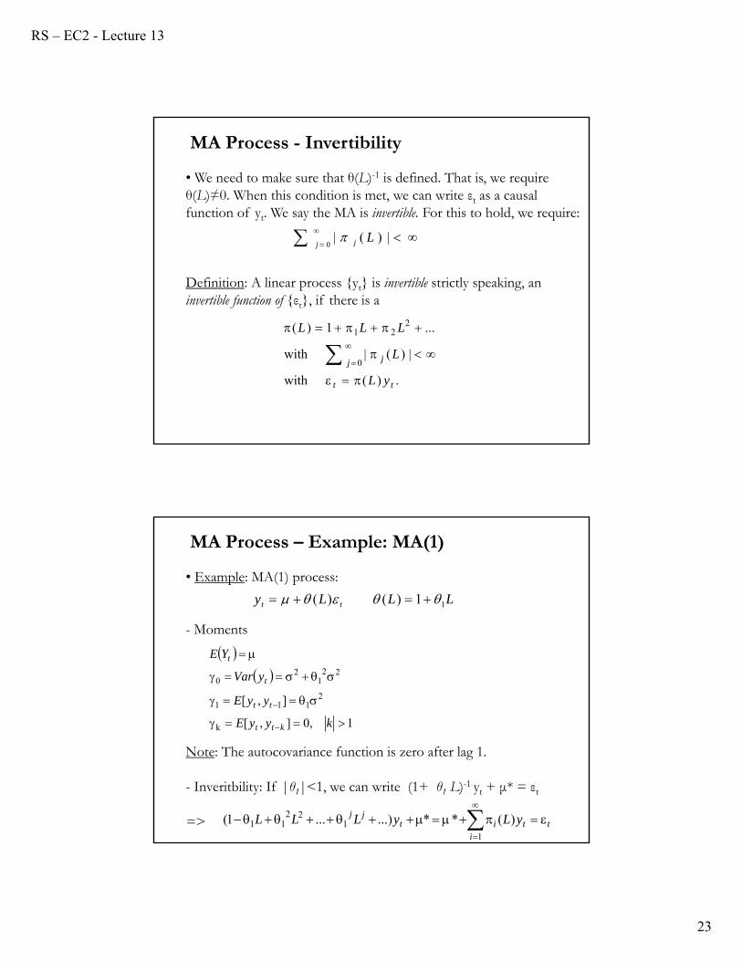
• We need to make sure that θ(L)-1 is defined. That is, we require θ(L)≠0. When this condition is met, we can write εt as a causal function of yt. We say the MA is invertible. For this to hold, we require:

Definition: A linear process {yt} is invertible strictly speaking, an invertible function of {εt}, if there is a

MA Process - Invertibility

0|)(|

j j L

.)(with

|)(|with

...1)(

0

221

tt

j j

yL

L

LLL

• Example: MA(1) process:

- Moments

Note: The autocovariance function is zero after lag 1.

- Inveritbility: If |θ1|<1, we can write (1+ θ1 L)-1 yt + μ* = εt

=>

MA Process – Example: MA(1)

1

122

11 )(**...)...1(i

ttitjj yLyLLL

LLLy tt 11)()(

1,0],[

],[

k

2111

221

20

kyyE

yyE

yVar

YE

ktt

tt

t

t


24

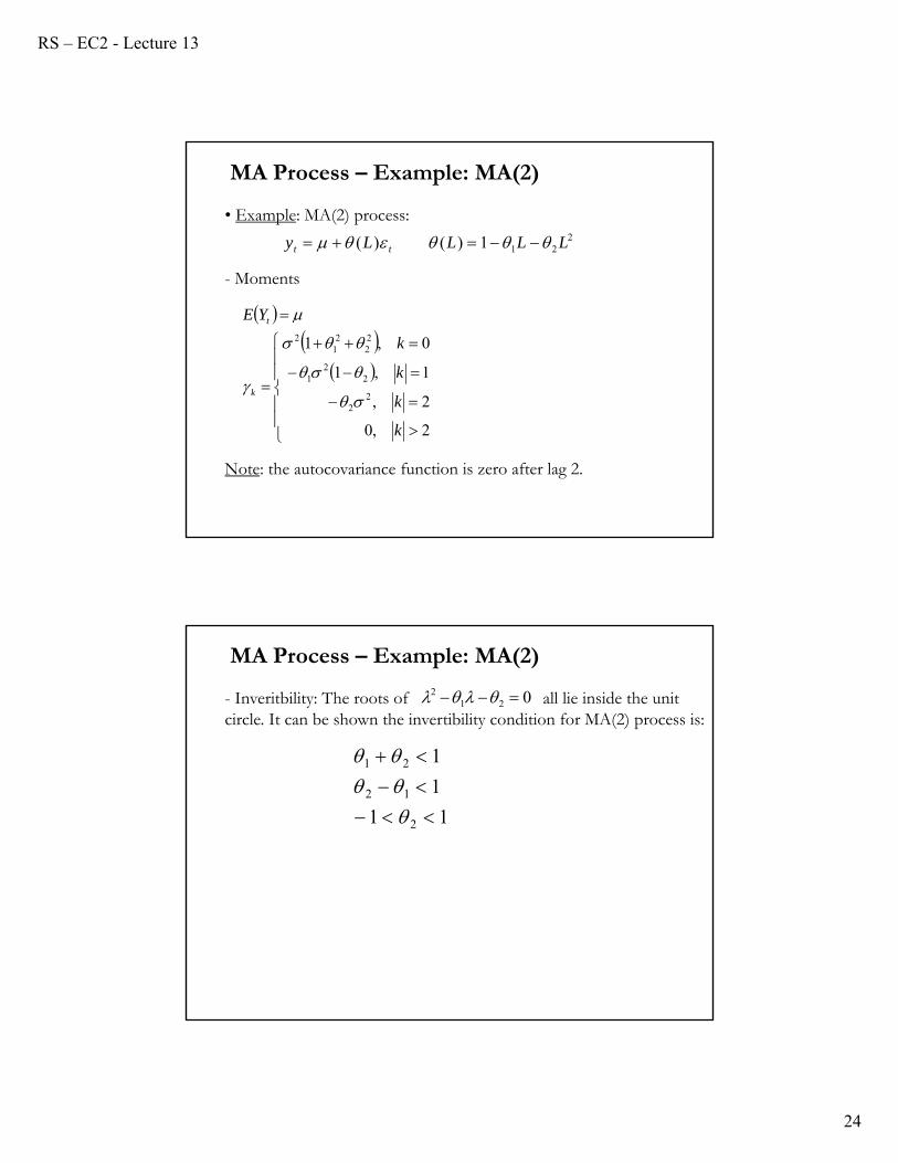
• Example: MA(2) process:

- Moments

Note: the autocovariance function is zero after lag 2.


2211)()( LLLLy tt

2,0

2,

1,1

0,1

22

22

1

22

21

2

k

k

k

k

YE

k

t

- Inveritbility: The roots of all lie inside the unit circle. It can be shown the invertibility condition for MA(2) process is:


0212

11

1

1

2

12

21


25

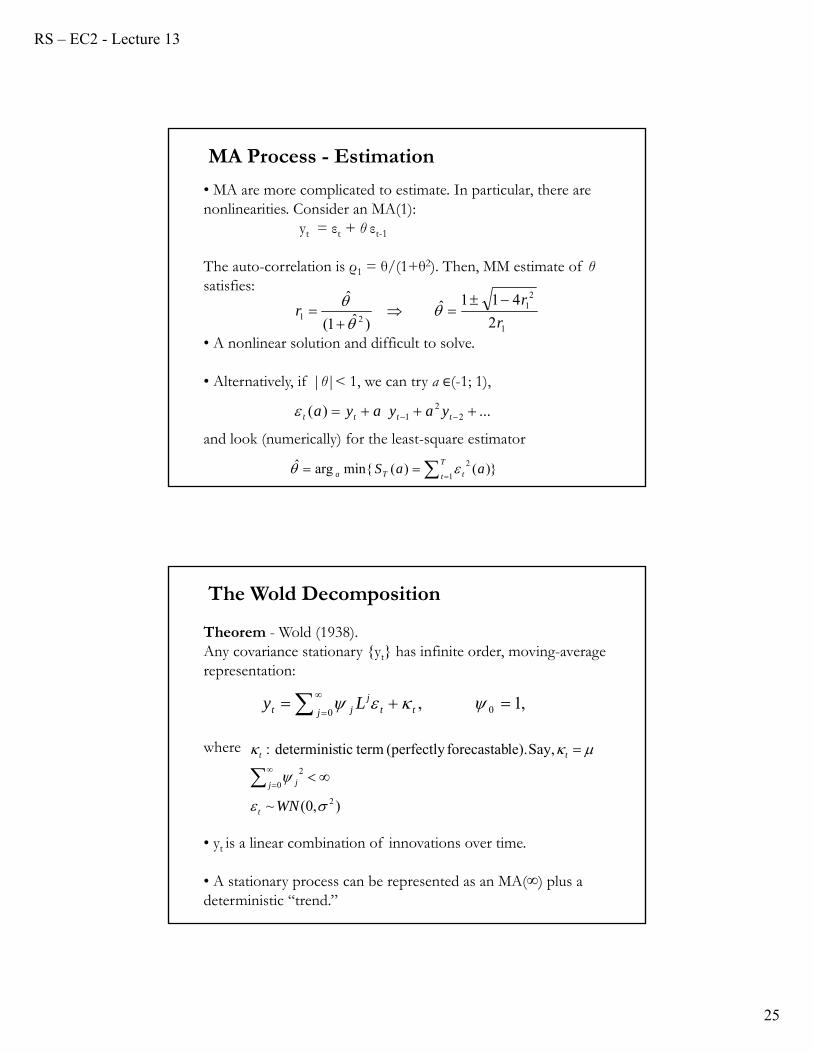
• MA are more complicated to estimate. In particular, there are nonlinearities. Consider an MA(1):

yt = εt + θ εt-1

The auto-correlation is ρ1 = θ/(1+θ2). Then, MM estimate of θsatisfies:

• A nonlinear solution and difficult to solve.

• Alternatively, if |θ|< 1, we can try a ∈(-1; 1),

and look (numerically) for the least-square estimator

MA Process - Estimation

1

21

21 2

411ˆ)ˆ1(

ˆ

r

rr

...)( 22

1 tttt yayaya

})()(min{argˆ1

2

T

t tTa aaS

Theorem - Wold (1938).Any covariance stationary {yt} has infinite order, moving-average representation:

where

• yt is a linear combination of innovations over time.

• A stationary process can be represented as an MA(∞) plus a deterministic “trend.”

The Wold Decomposition

),0(~

Say, le).forecastab (perfectly termticdeterminis:

2

0

2

WNt

j j

tt

,1, 00

tj t

jjt Ly


26

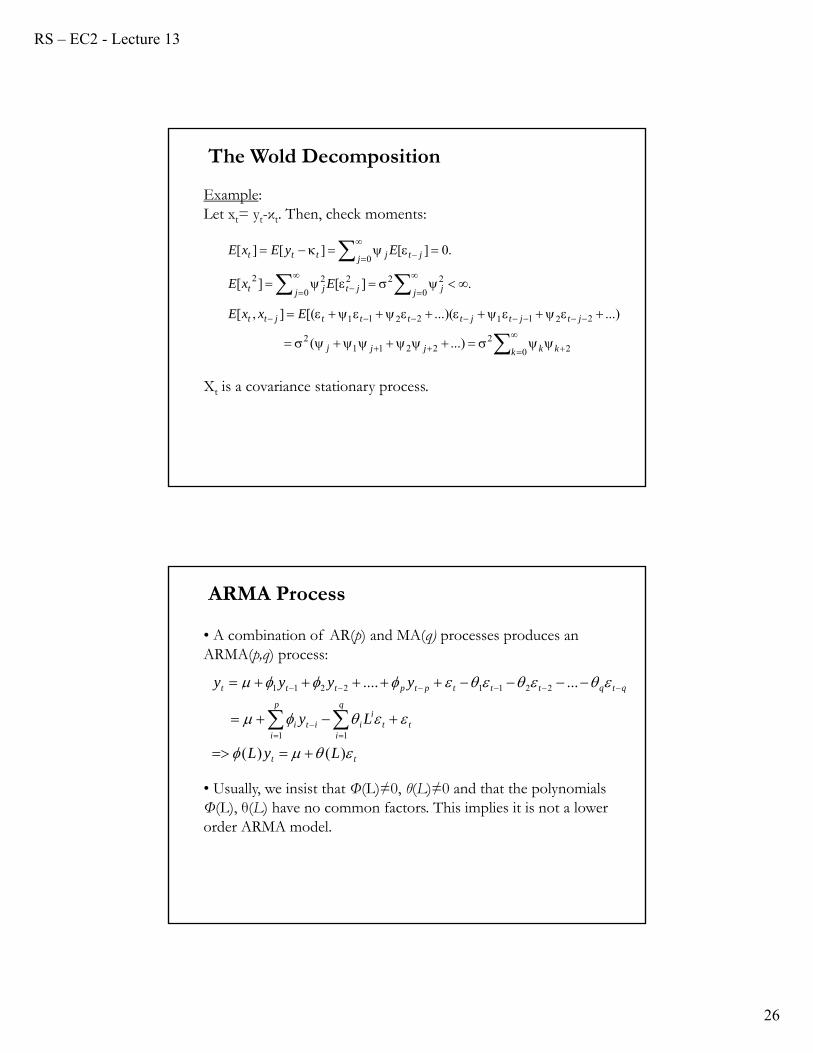
Example:Let xt= yt-κt. Then, check moments:

Xt is a covariance stationary process.

The Wold Decomposition

0 22

22112

22112211

0

22

0

222

0

...)(

...)...)([(],[

.][][

.0][][][

k kkjjj

jtjtjttttjtt

j jj jtjt

j jtjttt

ExxE

ExE

EyExE

• A combination of AR(p) and MA(q) processes produces an ARMA(p,q) process:

• Usually, we insist that Φ(L)≠0, θ(L)≠0 and that the polynomials Φ(L), θ(L) have no common factors. This implies it is not a lower order ARMA model.

ARMA Process

tt

t

q

it

iiit

p

ii

qtqtttptpttt

LyL

Ly

yyyy

)()(

.......

11

22112211


27

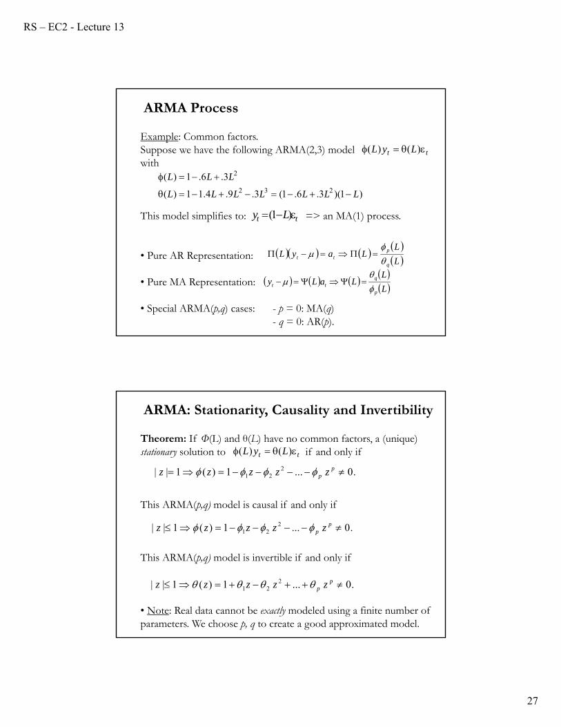
Example: Common factors. Suppose we have the following ARMA(2,3) modelwith

This model simplifies to: => an MA(1) process.

• Pure AR Representation:

• Pure MA Representation:

• Special ARMA(p,q) cases: - p = 0: MA(q)- q = 0: AR(p).

tt Ly )1(

tt LyL )()(

)1)(3.6.1(3.9.4.11)(

3.6.1)(232

2

LLLLLLL

LLL

ARMA Process

L

LLayL

q

ptt

L

LLaLy

p

qtt

Theorem: If Φ(L) and θ(L) have no common factors, a (unique) stationary solution to if and only if

This ARMA(p,q) model is causal if and only if

This ARMA(p,q) model is invertible if and only if

• Note: Real data cannot be exactly modeled using a finite number of parameters. We choose p, q to create a good approximated model.

tt LyL )()(

ARMA: Stationarity, Causality and Invertibility

.0...1)(1|| 221 p

p zzzzz

.0...1)(1|| 221 p

p zzzzz

.0...1)(1|| 221 p

p zzzzz


28

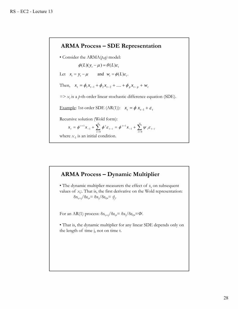
• Consider the ARMA(p,q) model:

Let

Then,

=> xt is a p-th-order linear stochastic difference equation (SDE).

Example: 1st-order SDE (AR(1)):

Recursive solution (Wold form):

where x-1 is an initial condition.

ARMA Process – SDE Representation

)())(( tt LyL

.)(and tttt Lwyx

tptpttt wxxxx ....2211

ttt xx 1

iti

it

iti

ttt xxx

0

11

01

1

• The dynamic multiplier measurers the effect of εt on subsequent values of xt:. That is, the first derivative on the Wold representation:

δxt+j/δεt,= δxj/δε0,= ψj.

For an AR(1) process: δxt+j/δεt,= δxj/δε0,=Φj.

• That is, the dynamic multiplier for any linear SDE depends only on the length of time j, not on time t.

ARMA Process – Dynamic Multiplier


29

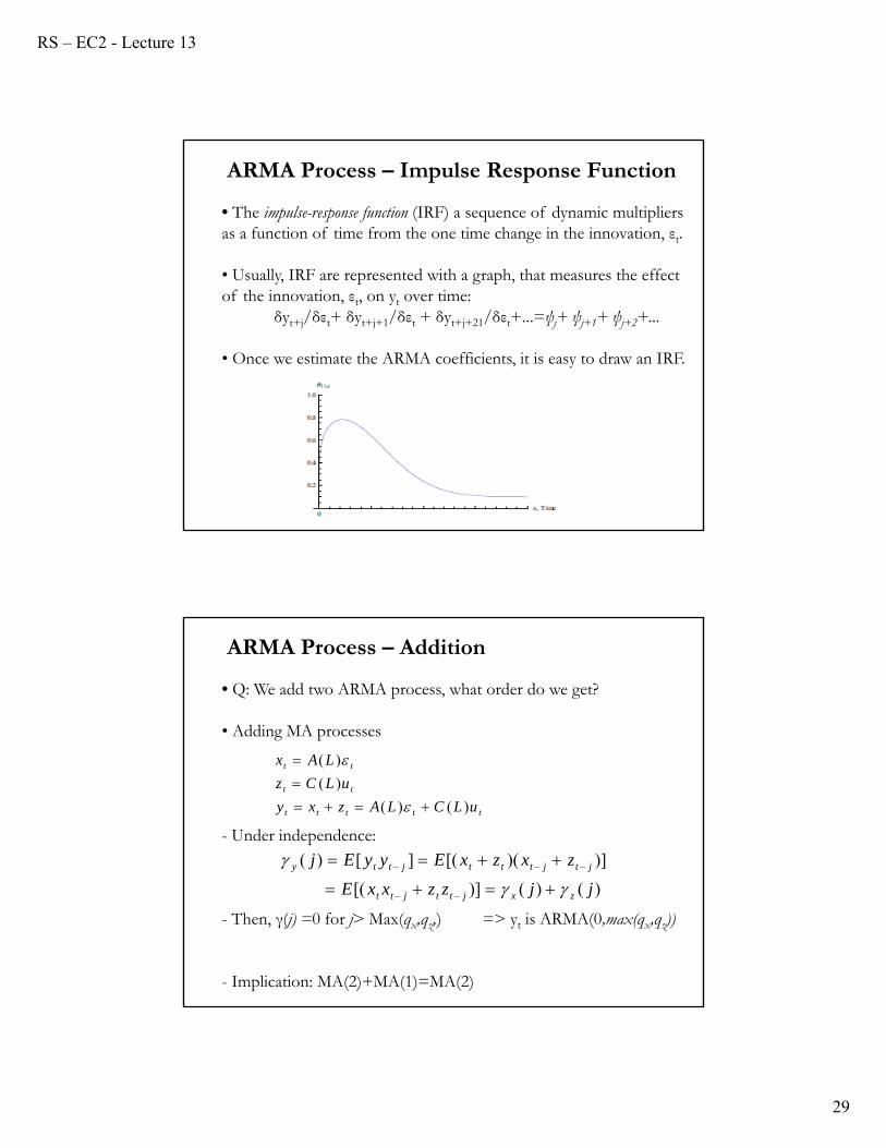
• The impulse-response function (IRF) a sequence of dynamic multipliers as a function of time from the one time change in the innovation, εt.

• Usually, IRF are represented with a graph, that measures the effect of the innovation, εt, on yt over time:

δyt+j/δεt+ δyt+j+1/δεt + δyt+j+21/δεt+...=ψj+ ψj+1+ ψj+2+...

• Once we estimate the ARMA coefficients, it is easy to draw an IRF.

ARMA Process – Impulse Response Function

• Q: We add two ARMA process, what order do we get?

• Adding MA processes

- Under independence:

- Then, γ(j) =0 for j> Max(qx,qz,) => yt is ARMA(0,max(qx,qz))

- Implication: MA(2)+MA(1)=MA(2)

ARMA Process – Addition

ttttt

tt

tt

uLCLAzxy

uLCz

LAx

)( )(

)(

)(

)()()][(

)])([(][)(

jjzzxxE

zxzxEyyEj

zxjttjtt

jtjtttjtty


30

• Q: We add two ARMA process, what order do we get?

• Adding AR processes

- Rewrite system as:

- Then, yt is ARMA(px+pz ,max(px,pz))

ARMA Process – Addition

?

))(1(

))(1(

ttt

tt

tt

zxy

uzLC

xLA

])( )([))(1( ))(1())(1))((1(

))(1())(1))((1(

))(1())(1))((1(

ttttttt

tt

tt

uLALCuuLALCyLCLA

uLAzLCLA

LCxLALC

Documents

Lecture 13 Time Series: Stationarity, AR(p) & MA(q) · Lecture 13 Time Series: Stationarity, AR(p) ... ergodic theorem will give us a counterpart to the LLN. ... Difficult to prove