Washington University in St. Louis Washington University in St. Louis

Washington University Open Scholarship Washington University Open Scholarship

Engineering and Applied Science Theses & Dissertations McKelvey School of Engineering

Spring 5-15-2016

Learning with Scalability and Compactness Learning with Scalability and Compactness

Wenlin Chen Washington University in St. Louis

Follow this and additional works at: https://openscholarship.wustl.edu/eng_etds

Part of the Computer Sciences Commons

Recommended Citation Recommended Citation Chen, Wenlin, "Learning with Scalability and Compactness" (2016). Engineering and Applied Science Theses & Dissertations. 155. https://openscholarship.wustl.edu/eng_etds/155

This Dissertation is brought to you for free and open access by the McKelvey School of Engineering at Washington University Open Scholarship. It has been accepted for inclusion in Engineering and Applied Science Theses & Dissertations by an authorized administrator of Washington University Open Scholarship. For more information, please contact digital@wumail.wustl.edu.

WASHINGTON UNIVERSITY IN ST. LOUIS

School of Engineering and Applied ScienceDepartment of Computer Science and Engineering

Dissertation Examination Committee:Yixin Chen, Chair

Sanmay DasYasutaka Furukawa

Roman GarnettNan Lin

Kilian Q. Weinberger

Learning with Scalability and Compactnessby

Wenlin Chen

A dissertation presented to theGraduate School of Arts & Sciences

of Washington University inpartial fulfillment of the

requirements for the degreeof Doctor of Philosophy

May 2016St. Louis, Missouri

c© 2016, Wenlin Chen

Contents

List of Tables . . . . . . . . . . . . . . . . . . . . . . . . . . . . . . . . . . . . . . . iv

List of Figures . . . . . . . . . . . . . . . . . . . . . . . . . . . . . . . . . . . . . . v

Acknowledgments . . . . . . . . . . . . . . . . . . . . . . . . . . . . . . . . . . . . vii

Abstract . . . . . . . . . . . . . . . . . . . . . . . . . . . . . . . . . . . . . . . . . . x

1 Introduction . . . . . . . . . . . . . . . . . . . . . . . . . . . . . . . . . . . . . . 11.1 Supervised learning . . . . . . . . . . . . . . . . . . . . . . . . . . . . . . . . 2

1.1.1 Data for supervised learning problems . . . . . . . . . . . . . . . . . 21.1.2 Linear classification models . . . . . . . . . . . . . . . . . . . . . . . 4

1.2 Neural networks . . . . . . . . . . . . . . . . . . . . . . . . . . . . . . . . . . 71.2.1 From single layer to multiple layers . . . . . . . . . . . . . . . . . . . 71.2.2 Backpropagation . . . . . . . . . . . . . . . . . . . . . . . . . . . . . 10

1.3 Unsupervised learning - maximum variance unfolding (MVU) . . . . . . . . . 121.4 Motivations . . . . . . . . . . . . . . . . . . . . . . . . . . . . . . . . . . . . 14

1.4.1 Scalability of MVU . . . . . . . . . . . . . . . . . . . . . . . . . . . . 171.4.2 Redundancy in neural networks . . . . . . . . . . . . . . . . . . . . . 18

2 Compressing Heuristics with Graph Embedding . . . . . . . . . . . . . . . 202.1 Maximum variance correction for speeding up MVU . . . . . . . . . . . . . . 21

2.1.1 Introduction . . . . . . . . . . . . . . . . . . . . . . . . . . . . . . . . 212.1.2 Background and related work . . . . . . . . . . . . . . . . . . . . . . 232.1.3 Method . . . . . . . . . . . . . . . . . . . . . . . . . . . . . . . . . . 252.1.4 Experimental results . . . . . . . . . . . . . . . . . . . . . . . . . . . 332.1.5 Conclusion . . . . . . . . . . . . . . . . . . . . . . . . . . . . . . . . . 40

2.2 Goal-oriented Euclidean heuristics - a refined Euclidean heuristic . . . . . . . 402.2.1 Introduction . . . . . . . . . . . . . . . . . . . . . . . . . . . . . . . . 402.2.2 Goal-oriented Euclidean heuristic . . . . . . . . . . . . . . . . . . . . 412.2.3 State heuristic enhancement . . . . . . . . . . . . . . . . . . . . . . . 462.2.4 Experimental results . . . . . . . . . . . . . . . . . . . . . . . . . . . 492.2.5 Conclusions . . . . . . . . . . . . . . . . . . . . . . . . . . . . . . . . 52

3 Compressing Deep Learning Models . . . . . . . . . . . . . . . . . . . . . . . 54

ii

3.1 Compressing neural networks with the hashing trick . . . . . . . . . . . . . . 543.1.1 Introduction . . . . . . . . . . . . . . . . . . . . . . . . . . . . . . . . 543.1.2 Feature Hashing . . . . . . . . . . . . . . . . . . . . . . . . . . . . . . 573.1.3 Notation . . . . . . . . . . . . . . . . . . . . . . . . . . . . . . . . . . 583.1.4 HashedNets . . . . . . . . . . . . . . . . . . . . . . . . . . . . . . . . 593.1.5 Related Work . . . . . . . . . . . . . . . . . . . . . . . . . . . . . . . 653.1.6 Experimental Results . . . . . . . . . . . . . . . . . . . . . . . . . . . 683.1.7 Conclusion . . . . . . . . . . . . . . . . . . . . . . . . . . . . . . . . . 73

3.2 Compressing convolutional neural network in the frequency domain . . . . . 743.2.1 Introduction . . . . . . . . . . . . . . . . . . . . . . . . . . . . . . . . 743.2.2 Background . . . . . . . . . . . . . . . . . . . . . . . . . . . . . . . . 763.2.3 Frequency-Sensitive Hashed Nets . . . . . . . . . . . . . . . . . . . . 773.2.4 Related Work . . . . . . . . . . . . . . . . . . . . . . . . . . . . . . . 823.2.5 Experimental Results . . . . . . . . . . . . . . . . . . . . . . . . . . . 833.2.6 Conclusion . . . . . . . . . . . . . . . . . . . . . . . . . . . . . . . . . 90

4 Deep learning Meets Embedding:An Application to Model Compression . . . . . . . . . . . . . . . . . . . . . 914.1 Introduction . . . . . . . . . . . . . . . . . . . . . . . . . . . . . . . . . . . . 924.2 Method . . . . . . . . . . . . . . . . . . . . . . . . . . . . . . . . . . . . . . 95

4.2.1 Categorical feature embedding . . . . . . . . . . . . . . . . . . . . . . 964.2.2 Remaining layers . . . . . . . . . . . . . . . . . . . . . . . . . . . . . 974.2.3 Training . . . . . . . . . . . . . . . . . . . . . . . . . . . . . . . . . . 984.2.4 Visualization . . . . . . . . . . . . . . . . . . . . . . . . . . . . . . . 98

4.3 Discussion . . . . . . . . . . . . . . . . . . . . . . . . . . . . . . . . . . . . . 994.3.1 Compressing one-hot encoding . . . . . . . . . . . . . . . . . . . . . . 994.3.2 Feature hashing for CENN . . . . . . . . . . . . . . . . . . . . . . . . 1024.3.3 Dimensionality of embeddings . . . . . . . . . . . . . . . . . . . . . . 1044.3.4 Relation to factorization machines . . . . . . . . . . . . . . . . . . . . 105

4.4 Related work . . . . . . . . . . . . . . . . . . . . . . . . . . . . . . . . . . . 1064.5 Experimental results . . . . . . . . . . . . . . . . . . . . . . . . . . . . . . . 109

4.5.1 Experimental settings . . . . . . . . . . . . . . . . . . . . . . . . . . . 1094.5.2 Evaluation on UCI datasets . . . . . . . . . . . . . . . . . . . . . . . 1114.5.3 Classification with many categories . . . . . . . . . . . . . . . . . . . 1124.5.4 Visualization . . . . . . . . . . . . . . . . . . . . . . . . . . . . . . . 115

4.6 Conclusions . . . . . . . . . . . . . . . . . . . . . . . . . . . . . . . . . . . . 116

5 Conclusions . . . . . . . . . . . . . . . . . . . . . . . . . . . . . . . . . . . . . . 118

References . . . . . . . . . . . . . . . . . . . . . . . . . . . . . . . . . . . . . . . . . 121

iii

List of Tables

2.1 Relative A∗ search speedup over the differential heuristic (in expanded nodes)and embedding variance (×105). . . . . . . . . . . . . . . . . . . . . . . . . 35

2.2 Training time for MVU [145] and MVC, reported after initialization, the first10 iterations (MVC-10), and after convergence. . . . . . . . . . . . . . . . . 38

2.3 Speedup of various methods as compared to the differential heuristic. . . . . . . . 512.4 The total number of states (n), size of goal sets (ng), and training time for various

heuristics on different problems. For EH+SHE and GOEH+SHE, we also report

the additional time for computing SHE. . . . . . . . . . . . . . . . . . . . . . . 52

3.1 Test error rates (in %) with a compression factor of 18

across all data sets.Best results are printed in blue. . . . . . . . . . . . . . . . . . . . . . . . . . 69

3.2 Test error rates (in %) with a compression factor of 164

across all data sets.Best results are printed in blue. . . . . . . . . . . . . . . . . . . . . . . . . . 69

3.3 Network architecture. C: Convolution. RL: ReLu. MP: Max-pooling. DO:Dropout. FC: Fully-connected. The number of parameters in the fully-connected layer is specific to 32×32 input images and varies with the numberof classes, either 10 or 100 depending on the dataset. . . . . . . . . . . . . . 85

3.4 Test error rates (in %) with compression factors 1/16 and 1/64. Convolutionallayers were compressed by the indicated methods (DropFilt, DropFreq, LRD,HashedNets, and FreshNets), with no convolutional layer compression appliedto CNN. The fully connected layer is compressed by HashNets for all methods,including CNN. . . . . . . . . . . . . . . . . . . . . . . . . . . . . . . . . . . 85

4.1 Test errors of various methods on various UCI datasets (in %). . . . . . . . . 1094.2 An description of the triptype dataset . . . . . . . . . . . . . . . . . . . . . . 1124.3 Test error performance on the triptype dataset (in %). . . . . . . . . . . . . 1134.4 Results of k-means clustering on the learned embeddings in CENN. . . . . . 114

iv

List of Figures

1.1 Examples from CIFAR-10 dataset . . . . . . . . . . . . . . . . . . . . . . . . 31.2 An example feature vector . . . . . . . . . . . . . . . . . . . . . . . . . . . . 41.3 SVM classification in 2-dimensional space. . . . . . . . . . . . . . . . . . . . 61.4 Loss functions . . . . . . . . . . . . . . . . . . . . . . . . . . . . . . . . . . . 71.5 Architecture of neural networks . . . . . . . . . . . . . . . . . . . . . . . . . 81.6 Activation functions. . . . . . . . . . . . . . . . . . . . . . . . . . . . . . . . 91.7 Maximum variance unfolding illustrated on a Swiss roll graph, embedded into

a 2-dimensional Euclidean space. . . . . . . . . . . . . . . . . . . . . . . . . 13

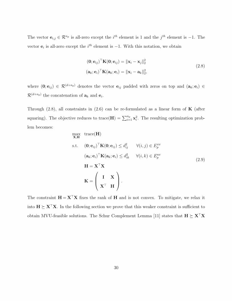
2.1 Drawing of a patch with inner and anchor points. . . . . . . . . . . . . . . . 282.2 Visualization of several MVC iterations on the 5-puzzle data set (m = 30).

The edges are colored proportional to their relative admissibility gap ξ, asdefined in (2.15). The top left image shows the (rescaled) Isomap initialization.The successive graphs show that MVC decreases the edge admissibility gapsand increases the variance with each iteration (indicated in the title of eachsubplot) until it converges to the same variance as the MVU solution (bottomright). . . . . . . . . . . . . . . . . . . . . . . . . . . . . . . . . . . . . . . . 34

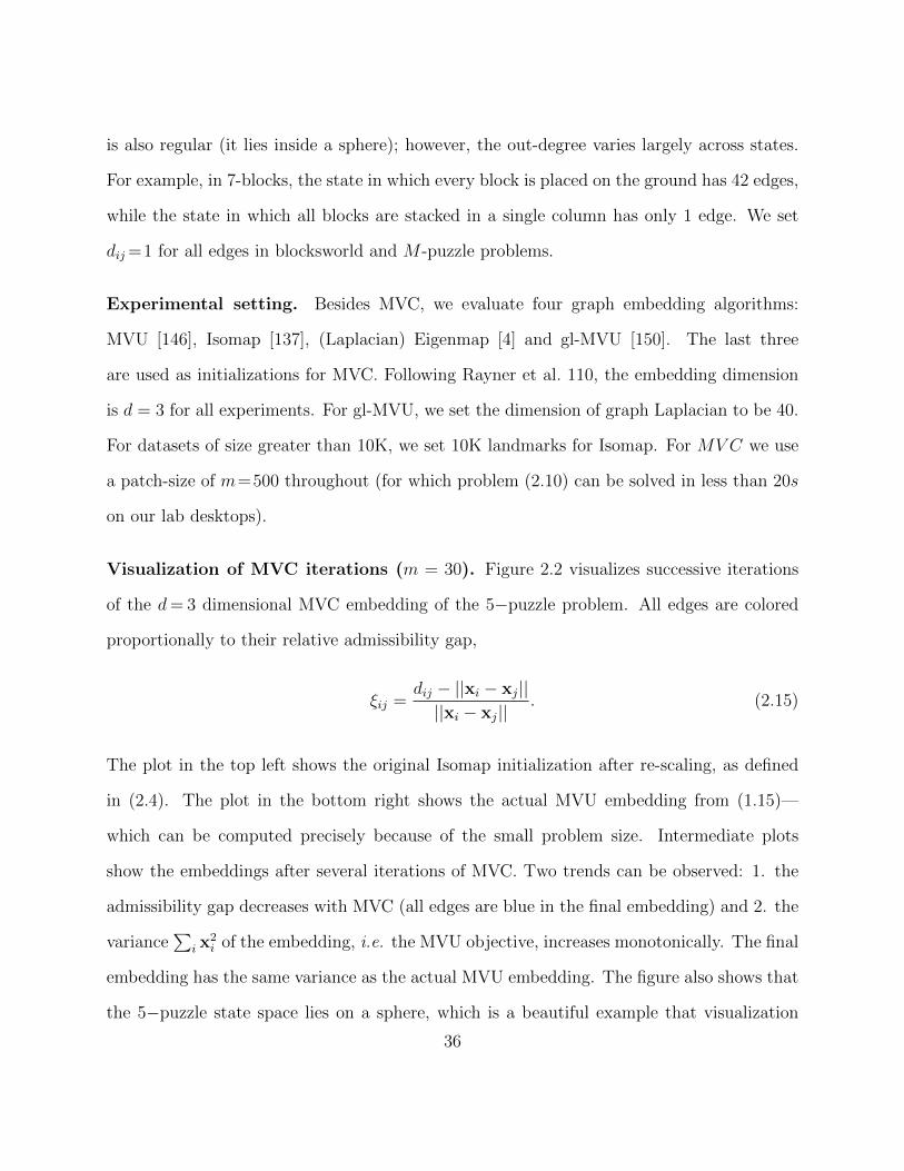
2.3 (Left) the embedding variance of 6-blocksworld plotted over 30 MVC itera-tions. The variance increases monotonically and even outperforms the actualMVU embedding [146] after only a few iterations. (Right) the number of ex-panded nodes in A∗ search as a function of the optimal solution length. AllMVC solutions strictly outperform the Differential Heuristic (diff ) and evenexpand fewer nodes than MVU. . . . . . . . . . . . . . . . . . . . . . . . . . 37

2.4 EH and GOEH embeddings (d = 3) illustrated on a 5-puzzle problem. Goalstates are colored in red, others in green. In this spherical embedding in theleft figure, the Euclidean distance is a bad approximation for distant states.GOEH deforms the embedding to better reflect the spherical distance fromfar away states to the goal states—at the cost of shrinkage between non-goalstates. . . . . . . . . . . . . . . . . . . . . . . . . . . . . . . . . . . . . . . . 44

2.5 The number of expanded nodes in the optimal search as a function of theoptimal solution length. For EH+SHE and GOEH+SHE, B′ search is usedand the re-opened nodes are counted as new expansions. . . . . . . . . . . . 48

v

3.1 An illustration of a neural network with random weight sharing under com-pression factor 1

4. The 16+9 = 25 virtual weights are compressed into 6 real

weights. The colors represent matrix elements that share the same weight value. 603.2 Test error rates under varying compression factors with 3-layer networks on

mnist (left) and rot (right). . . . . . . . . . . . . . . . . . . . . . . . . . . 683.3 Test error rates under varying compression factors with 5-layer networks on

mnist (left) and rot (right). . . . . . . . . . . . . . . . . . . . . . . . . . . 683.4 Test error rates with fixed storage but varying expansion factors on mnist

with 3 layers (left) and 5 layers (right). . . . . . . . . . . . . . . . . . . . . 703.5 A schematic illustration of FreshNets. Two spatial filters are re-constructed

from the frequency weights in vector w. The frequency weights are accessedwith two hash functions and then transformed to the spatial domain. Thevector w is partitioned into sub-vectors wj shared by all entries with similarfrequency (corresponding to index sum j = j1 + j2). Colors indicate whichhash bucket was accessed. . . . . . . . . . . . . . . . . . . . . . . . . . . . . 78

3.6 An example of a filter in spatial (left) and frequency domain (right). . . . . 813.7 Test error rates at varying compression levels for datasets cifar10 (left) and

rot (right). . . . . . . . . . . . . . . . . . . . . . . . . . . . . . . . . . . . . 863.8 Results with different frequency sensitive compression schemes, each adopt-

ing a different beta distribution as the compression rate for each frequency.The inner figure shows normalized test error of each scheme on cifar10 withthe beta distribution hyper-parameters. The outer figure depicts the corre-sponding beta distributions. The setting α = 0.2, β = 2.5 (blue line), whichcompresses low frequencies the least and high frequencies the most, yieldslowest error. . . . . . . . . . . . . . . . . . . . . . . . . . . . . . . . . . . . 87

3.9 Visualization of filters learning on mnist in (a) an uncompressed CNN, (b) aCNN compressed with FreshNets, and (c) a CNN compressed with Hashed-Nets (compression rate 1/16 in both (b) and (c)). FreshNets preserves thesmoothness of the filters, whereas HashedNets does not. . . . . . . . . . . . . 89

4.1 The architecture of CENN for classification. . . . . . . . . . . . . . . . . . . 954.2 One-hot encoding, mathematically Ur, is equivalent to the transformation

performed in CENN that retrieves embeddings and does element-wise sum. . 1014.3 The embeddings for the “Department Description” feature . . . . . . . . . . 113

vi

Acknowledgments

First and foremost, I would like to express my special appreciation and sincerest gratitude

to my advisor Yixin Chen. None of the work described in this dissertation would have been

possible without his guidance and support. I very much enjoy discussing ideas with him as

I always get valuable advice and inspiration from him. I especially thank him for giving me

much academic freedom during my entire course of PhD study, which allows me to work on

any research topic I like and collaborate with people inside or outside the lab. I could not

have imagined having a better advisor and mentor for my Ph.D study.

I would like to thank Kilian Q. Weinberger for co-supervising me and introducing me into the

field of machine learning. The joy and enthusiasm he has for machine learning was always

contagious and motivational for me. I am also thankful for the excellent example he has

provided as a successful researcher.

I would also like to thank the rest of my dissertation committee, Sanmay Das, Roman

Garnett, Yasutaka Furukawa and Nan Lin for their valuable comments and suggestions to

this dissertation. I also thank them for hosting seminars and talks which keep me up-to-date

about the state-of-the-art research.

I would like to thank David Grangier, Michael Auli, Nicolas Mayoraz and Sally A. Goldman

for providing me with great internship opportunities at Facebook AI Research and Google

vii

Research. Their great supervision not only gives me two wonderful summers, but also helps

shape my long-term career path after graduation.

I would like to thank my friends and colleagues Minmin Chen, Zheng Chen, Zhicheng Cui,

Jake Gardener, Yujie He, Gao Huang, Matt Kusner, Qiang Lu, Gustavo Malkomes, Yi Mao,

Yu Sun, Paras Tiwari, Stephen Tyree, Wenlin Wang, Yuan Wang, James Wilson, Eddie Xu,

Muhan Zhang and Quan Zhou for bouncing off ideas, discussing papers, collaborating on

projects, hanging out together and all the time we have shared.

I would like to thank my parents. Words cannot express how grateful I am to my father

Wenzhang Chen and my mother Guihua Hong for their unconditional love and support

during my life time. I would also like to thank my uncle Wenming Chen for buying me a

computer when I was a child, which brought me into the world of computer science.

Last but not the least, I would like to thank my beloved fiancee Ming Zou for her love,

support and encouragement. I could not have completed this journey without Ming by my

side. Because of her company, my PhD study is full of joys and happiness.

Wenlin Chen

Washington University in Saint Louis

May 2016

viii

Dedicated to my parents.

ix

ABSTRACT OF THE DISSERTATION

Learning with Scalability and Compactness

by

Wenlin Chen

Doctor of Philosophy in Computer Science

Washington University in St. Louis, 2016

Professor Yixin Chen, Chair

Artificial Intelligence has been thriving for decades since its birth. Traditional AI features

heuristic search and planning, providing good strategy for tasks that are inherently search-

based problems, such as games and GPS searching. In the meantime, machine learning,

arguably the hottest subfield of AI, embraces data-driven methodology with great success

in a wide range of applications such as computer vision and speech recognition. As a new

trend, the applications of both learning and search have shifted toward mobile and embed-

ded devices which entails not only scalability but also compactness of the models. Under

this general paradigm, we propose a series of work to address the issues of scalability and

compactness within machine learning and its applications on heuristic search.

We first focus on the scalability issue of memory-based heuristic search which is recently ame-

liorated by Maximum Variance Unfolding (MVU), a manifold learning algorithm capable of

learning state embeddings as effective heuristics to speed up A∗ search. Though achieving

unprecedented online search performance with constraints on memory footprint, MVU is no-

toriously slow on offline training. To address this problem, we introduce Maximum Variance

x

Correction (MVC), which finds large-scale feasible solutions to MVU by post-processing em-

beddings from any manifold learning algorithm. It increases the scale of MVU embeddings

by several orders of magnitude and is naturally parallel. We further propose Goal-oriented

Euclidean Heuristic (GOEH), a variant to MVU embeddings, which preferably optimizes the

heuristics associated with goals in the embedding while maintaining their admissibility. We

demonstrate unmatched reductions in search time across several non-trivial A∗ benchmark

search problems. Through these work, we bridge the gap between the manifold learning

literature and heuristic search which have been regarded as fundamentally different, leading

to cross-fertilization for both fields.

Deep learning has made a big splash in the machine learning community with its supe-

rior accuracy performance. However, it comes at a price of huge model size that might

involves billions of parameters, which poses great challenges for its use on mobile and em-

bedded devices. To achieve the compactness, we propose HashedNets, a general approach to

compressing neural network models leveraging feature hashing. At its core, HashedNets ran-

domly group parameters using a low-cost hash function, and share parameter value within

the group. According to our empirical results, a neural network could be 32x smaller with

little drop in accuracy performance. We further introduce Frequency-Sensitive Hashed Nets

(FreshNets) to extend this hashing technique to convolutional neural network by compressing

parameters in the frequency domain.

Compared with many AI applications, neural networks seem not graining as much popularity

as it should be in traditional data mining tasks. For these tasks, categorical features need

to be first converted to numerical representation in advance in order for neural networks

to process them. We show that a naıve use of the classic one-hot encoding may result in

gigantic weight matrices and therefore lead to prohibitively expensive memory cost in neural

xi

networks. Inspired by word embedding, we advocate a compellingly simple, yet effective

neural network architecture with category embedding. It is capable of directly handling both

numerical and categorical features as well as providing visual insights on feature similarities.

At the end, we conduct comprehensive empirical evaluation which showcases the efficacy and

practicality of our approach, and provides surprisingly good visualization and clustering for

categorical features.

xii

Chapter 1

Introduction

Artificial intelligence (AI) is a long-standing field and has been thriving for decades. Gen-

erally speaking, AI studies and designs intelligent agents that is capable of perceiving its

environment and taking actions to maximize its chances of success [119]. Traditional AI

features deduction, reasoning, planning and problem solving, which try to mimic the human

reasoning and thinking process when they are solving puzzles and logical problems. There-

fore, the developed method involves a huge amount of logic and domain knowledge. Different

than traditional AI, machine learning, arguably the hottest subfield of AI, develops the in-

telligent agents through learning from past experience and has been central to AI research

since the field’s inception1.

In this chapter, we first introduce supervised learning and unsupervised learning, which serve

as preliminaries for the following chapters of this dissertation. Then we point out the issues

of scalability and compactness that widely exists within machine learning, and motivate this

dissertation.

1https://en.wikipedia.org/wiki/Artificial_intelligence

1

1.1 Supervised learning

Depending on the type of problems, machine learning is further divided into several subfields.

As a brief introduction, we describe supervised learning in this section.

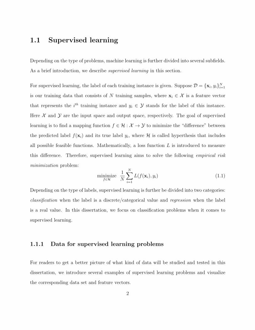
For supervised learning, the label of each training instance is given. Suppose D = {xi, yi}Ni=1

is our training data that consists of N training samples, where xi ∈ X is a feature vector

that represents the ith training instance and yi ∈ Y stands for the label of this instance.

Here X and Y are the input space and output space, respectively. The goal of supervised

learning is to find a mapping function f ∈ H : X → Y to minimize the “difference” between

the predicted label f(xi) and its true label yi, where H is called hyperthesis that includes

all possible feasible functions. Mathematically, a loss function L is introduced to measure

this difference. Therefore, supervised learning aims to solve the following empirical risk

minimization problem:

minimizef∈H

1

N

N∑i=1

L(f(xi), yi) (1.1)

Depending on the type of labels, supervised learning is further be divided into two categories:

classification when the label is a discrete/categorical value and regression when the label

is a real value. In this dissertation, we focus on classification problems when it comes to

supervised learning.

1.1.1 Data for supervised learning problems

For readers to get a better picture of what kind of data will be studied and tested in this

dissertation, we introduce several examples of supervised learning problems and visualize

the corresponding data set and feature vectors.

2

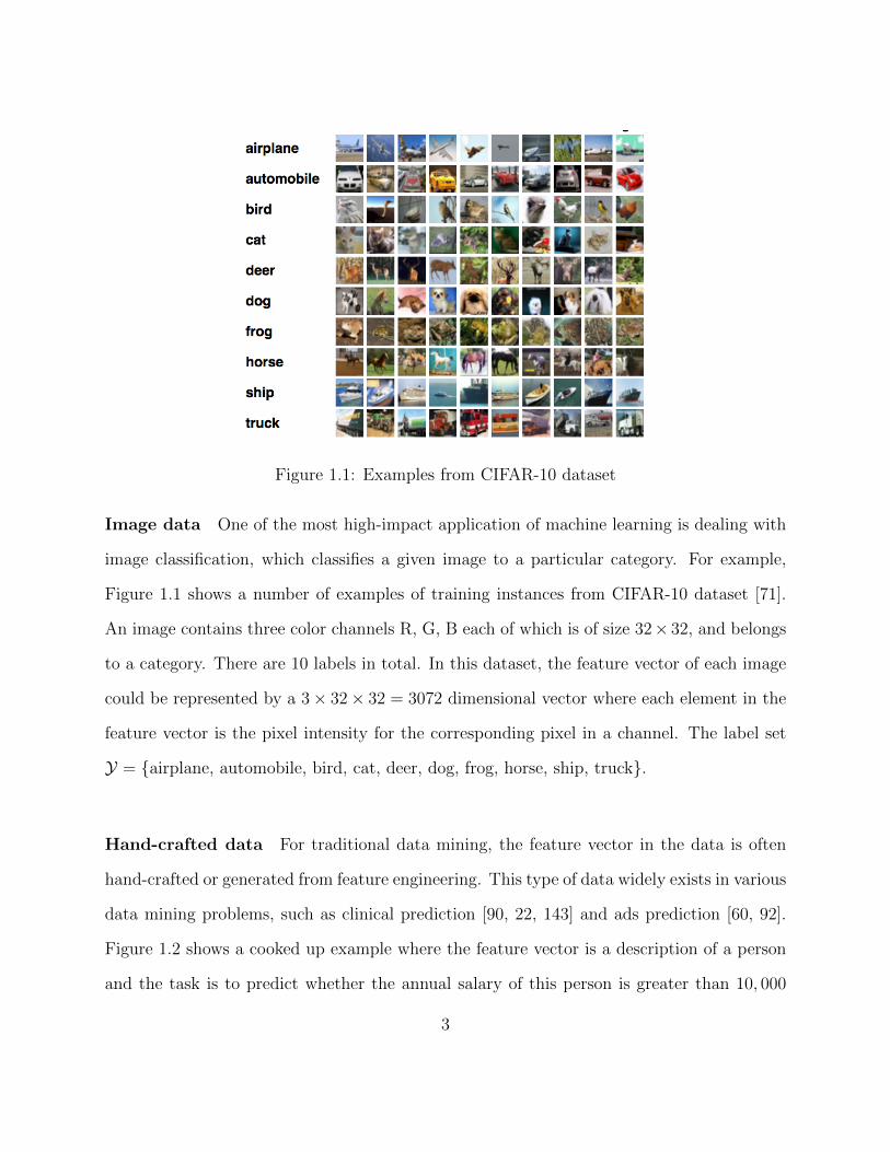
Figure 1.1: Examples from CIFAR-10 dataset

Image data One of the most high-impact application of machine learning is dealing with

image classification, which classifies a given image to a particular category. For example,

Figure 1.1 shows a number of examples of training instances from CIFAR-10 dataset [71].

An image contains three color channels R, G, B each of which is of size 32× 32, and belongs

to a category. There are 10 labels in total. In this dataset, the feature vector of each image

could be represented by a 3× 32× 32 = 3072 dimensional vector where each element in the

feature vector is the pixel intensity for the corresponding pixel in a channel. The label set

Y = {airplane, automobile, bird, cat, deer, dog, frog, horse, ship, truck}.

Hand-crafted data For traditional data mining, the feature vector in the data is often

hand-crafted or generated from feature engineering. This type of data widely exists in various

data mining problems, such as clinical prediction [90, 22, 143] and ads prediction [60, 92].

Figure 1.2 shows a cooked up example where the feature vector is a description of a person

and the task is to predict whether the annual salary of this person is greater than 10, 000

3

age, height, gender, degree, Country

xi = (24, 1.8, male, master, USA)

Figure 1.2: An example feature vector

dollars or not. The specialness about this type of data is that the feature vector contains

both numerical and categorical inputs. In this example, age and height are both numerical,

while gender, degree and country are categorical. For numerical classifiers, categorical input

should be first converted to a numerical representation. The most popular way to handle

categorical input is the so-called one-hot encoding, which will be discussed in Chapter 4.

1.1.2 Linear classification models

There are various classification models in the literature [58]. In this section, we only de-

scribe several linear classifiers for introduction purpose. Specifically, we focus on binary

classification where Y = {−1,+1}, and assume the feature vector x ∈ Rd is a numerical

representation.

Linear classifiers take the following general form:

f(x) = w>x + b (1.2)

where w ∈ Rd is the weight vector and b ∈ R is a bias term. Both are parameters in the

linear model and the learning process is to adjust the values of w and b such that the loss

function is minimized. Typically, a `2 regularization of the weight vector is added to the

4

objective function to alleviate the overfitting problem. Following Eq 1.1, we have that

minimizew∈Rd,b∈R

1

N

N∑i=1

L(w>xi + b, yi) + λ‖w‖2 (1.3)

where λ is a factor for `2 regularization and controls the tradeoff between loss function and

regularization. Different choices of the loss function L leads to different classifiers.

Logistic Regression. If we adopt the logistic loss as the loss function, Eq. 1.3 ends up

with a logistic regression. For logistic loss, L(u, v) = log (1 + exp (−uv)). Therefore, Eq. 1.3

can be rewritten as

minimizew∈Rd,b∈R

1

N

N∑i=1

log(1 + exp (−yi(w>xi + b)

)+ λ‖w‖2 (1.4)

Logistic regression not only predicts the label for the testing instances, but also providing

the probability of its prediction. Eq. 1.4 is also equivalent to maximizing the likelihood of

the dataset when the probability of yi being 1 is a sigmoid function of the linear score f(xi)

as follows:

p(y = 1|x) =1

1 + e−(w>x+b)(1.5)

Logistic regression could be easily extended to handle multinomial classification by having

multi-dimensional score functions. The probability of each class could be computed via a

softmax function which will be discussed in the later section.

Support vector machines (SVM). If the loss function is hinge loss, then Eq. 1.3 be-

comes a SVM solver. In particular, hinge loss L(u, v) = [1 − uv]+ is a piece-wise linear

function where [·]+ = max(0, ·). Combing with `2 regularization, Eq. 1.3 can be converted

5

Figure 1.3: SVM classification in 2-dimensional space.

to the following:

minimizew∈Rd,b∈R

1

N

N∑i=1

[1− yi(w>xi + b)

]+

+ λ‖w‖2 (1.6)

As shown in Figure 1.32, SVM has a clear geometry interpretation that its decision hyper-

plane has the largest distance to the nearest training data instances of any class, leading

to better generalization ability. The true power of SVM is its combination with the kernel

trick [122] which enables itself to handle nonlinear classification. It can also be used to

efficiently solve elastic nets [160].

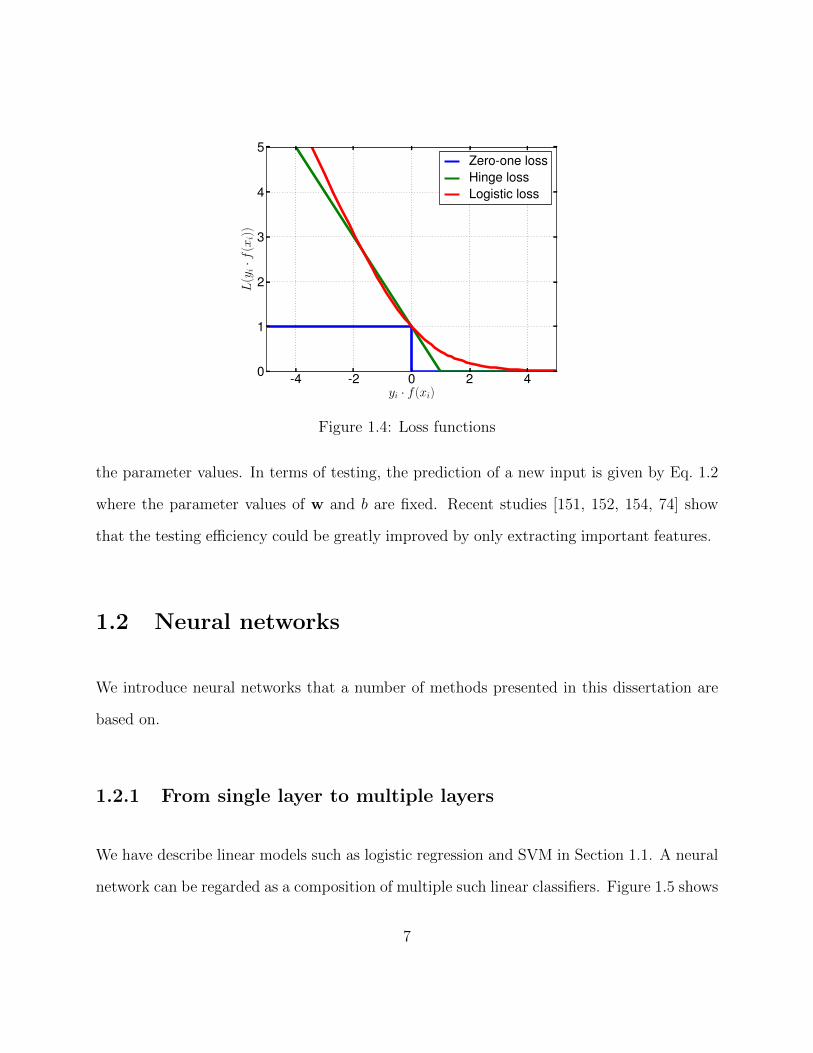
More on loss functions. Both hinge loss and logistic loss can be regarded as a proxy for

0-1 loss which is the training error of the dataset. Specifically, they are both upper bounds

of the 0-1 loss as shown in Figure 1.4. Therefore, minimizing these loss is approximately

reducing the training error of the dataset. Eq 1.4 and Eq 1.6 are both convex and could

be efficiently optimized with (subgradient) gradient descent [11] during training to finalize

2This figure is from https://en.wikipedia.org/wiki/Support_vector_machine

6

-4 -2 0 2 4yi · f (xi)

0

1

2

3

4

5

L(yi·f

(xi)

)

Zero-one lossHinge lossLogistic loss

Figure 1.4: Loss functions

the parameter values. In terms of testing, the prediction of a new input is given by Eq. 1.2

where the parameter values of w and b are fixed. Recent studies [151, 152, 154, 74] show

that the testing efficiency could be greatly improved by only extracting important features.

1.2 Neural networks

We introduce neural networks that a number of methods presented in this dissertation are

based on.

1.2.1 From single layer to multiple layers

We have describe linear models such as logistic regression and SVM in Section 1.1. A neural

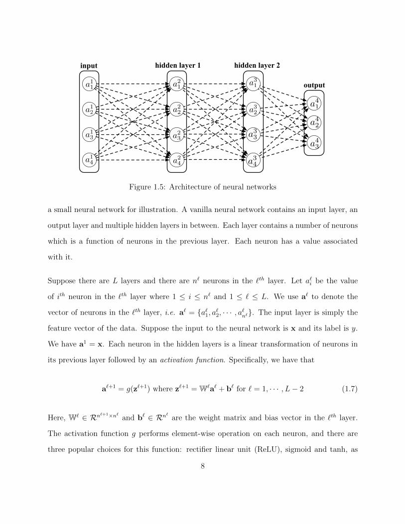
network can be regarded as a composition of multiple such linear classifiers. Figure 1.5 shows

7

input hidden layer 1

a11

a12

a13

a14 a2

4

a23

a22

a21 output

hidden layer 2

a31

a32

a34

a33

a43

a42

a41

Figure 1.5: Architecture of neural networks

a small neural network for illustration. A vanilla neural network contains an input layer, an

output layer and multiple hidden layers in between. Each layer contains a number of neurons

which is a function of neurons in the previous layer. Each neuron has a value associated

with it.

Suppose there are L layers and there are n` neurons in the `th layer. Let a`i be the value

of ith neuron in the `th layer where 1 ≤ i ≤ n` and 1 ≤ ` ≤ L. We use a` to denote the

vector of neurons in the `th layer, i.e. a` = {a`1, a`2, · · · , a`n`}. The input layer is simply the

feature vector of the data. Suppose the input to the neural network is x and its label is y.

We have a1 = x. Each neuron in the hidden layers is a linear transformation of neurons in

its previous layer followed by an activation function. Specifically, we have that

a`+1 = g(z`+1) where z`+1 = W`a` + b` for ` = 1, · · · , L− 2 (1.7)

Here, W` ∈ Rn`+1×n`and b` ∈ Rn`

are the weight matrix and bias vector in the `th layer.

The activation function g performs element-wise operation on each neuron, and there are

three popular choices for this function: rectifier linear unit (ReLU), sigmoid and tanh, as

8

-4 -2 0 2 4z

-1.5

-1.0

-0.5

0.0

0.5

1.0

1.5

2.0

2.5

3.0

g(z

)

ReLUsigmoidtanh

Figure 1.6: Activation functions.

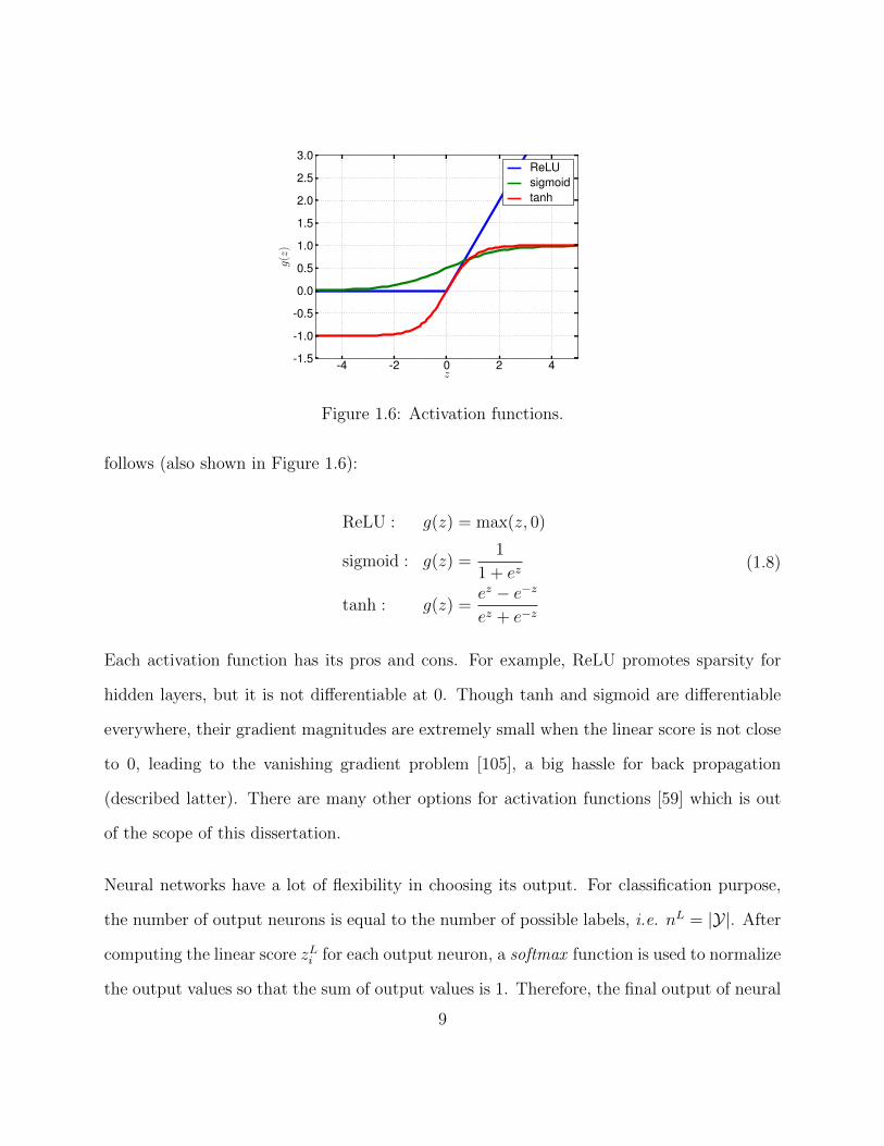
follows (also shown in Figure 1.6):

ReLU : g(z) = max(z, 0)

sigmoid : g(z) =1

1 + ez

tanh : g(z) =ez − e−zez + e−z

(1.8)

Each activation function has its pros and cons. For example, ReLU promotes sparsity for

hidden layers, but it is not differentiable at 0. Though tanh and sigmoid are differentiable

everywhere, their gradient magnitudes are extremely small when the linear score is not close

to 0, leading to the vanishing gradient problem [105], a big hassle for back propagation

(described latter). There are many other options for activation functions [59] which is out

of the scope of this dissertation.

Neural networks have a lot of flexibility in choosing its output. For classification purpose,

the number of output neurons is equal to the number of possible labels, i.e. nL = |Y|. After

computing the linear score zLi for each output neuron, a softmax function is used to normalize

the output values so that the sum of output values is 1. Therefore, the final output of neural

9

networks can be considered a multinomial distribution over possible labels. In particular, a

softmax function is a generalization of logistic regression described in Section 1.1 as follows:

aLi =ez

Li∑nL

k=1 ezLk

(1.9)

Why neural nets memory-consuming. The weight matrix of a neural network could

easily take up a huge amount of memory. For example, a neural net for mnist dataset [79],

a small image dataset about digits, usually has 784 input neurons, several layers of 1000

hidden units and an output layer of 10 neurons. In this case, a single hidden layer has a

weight matrix of size 1000× 1000, which consists of 1 million parameters in total. For larger

network, the memory consumption would be much larger.

1.2.2 Backpropagation

A softmax output is usually combined with a cross-entropy loss as the objective function

for parameter learning. For K-way multinomial classification, assume the output space of

labels Y = {1, 2, · · · , K}. For the ease of presentation, suppose there is only one training

instance in a batch. Let E be the negative log likelihood of an input, we have E = − log aLy =

−zLy + log(∑nL

k=1 ezLk ). And the goal is to minimize E for every input:

.minimizeW`,b`

− log aLy (1.10)

The parameters including the weight matrix and bias vector in each layer are learned via

gradient descent. However, computing the gradient of each parameter independently result

in a lot of redundant computation, which is why backpropagation [118] comes into play.

10

Backpropagation leverages the fact that the gradients of shallow layers can be expressed

as the gradients of higher layers. Let δ`i denote the gradient of the objective function in

Eq (1.10) over activation i in the `th layer. This gradient is usually referred as the error

term and play the role of propagating the gradient to shallow layers. When doing gradient

descent, we compute the following two types of gradients: the error term and the gradient

over parameters.

Error term. We compute the gradient of the objective function in Eq 1.9 over neurons. At

the top layer, we have

δLj =∂E

∂zLj= I(j, y)− aLj (1.11)

where I(j, y) = 1 when j = y and I(j, y) = 0 otherwise. For layers ` = 1, · · · , L− 1, we have

that

δ`j =∂E

∂z`j= (

n`+1∑i=1

Wijδ`+1i )g′(z`j) (1.12)

where W `ij is the element in the weight matrix indexed by (i, j).

Gradient over parameters. For parameter learning, our goal is to compute the gradient

over parameters W `i,j and b`i , which can be expressed by the error term as follows:

∂E

∂W `i,j

= a`jδ`+1i and

∂E

∂b`i= δ`+1

i (1.13)

Once we have the gradients over parameters, we can do stochastic gradient descent on the

parameters of the neural net until it converges. Usually, the training is coupled with other

techniques such as dropout, momentum and `2 regularization for preventing overfitting and

better convergence.

11

1.3 Unsupervised learning - maximum variance unfold-

ing (MVU)

Unsupervised learning is a machine learning task of exploring hidden patterns in the data.

Just as its name implies, unsupervised learning does not harness the supervision informa-

tion such as the label of the data. Unsupervised learning could be further divided into

several fields such as manifold learning/ graph embedding, clustering and statistical density

estimation. In this dissertation, we mainly focus on the graph embedding which aims to

embed a graph into a Euclidean space so that each node in a graph has a coordinate. There

are various graph embedding algorithms that are different in what properties are preserved

during the embedding. For example, Isomap [137] embeds the graph that most faithfully

preserves the shortest distance between any two nodes in the graph, while Laplacian eigen-

maps [4] preserves proximity relations, mapping nearby input nodes to nearby outputs. For

a more detailed survey we recommend [121]. The obtained embeddings can be used in a

wide range of down-stream applications such as visualization, classification or even heuristic

search which will be discussed in detail in Chapter 2.

In this section, we briefly review another graph embedding algorithm, Maximum Variance

Unfolding (MVU), which a big part of this dissertation is based on. MVU stems from

nonlinear dimensionality reduction [121] which maps high dimensional data points to low

dimensional embeddings while preserving certain properties about the manifold during the

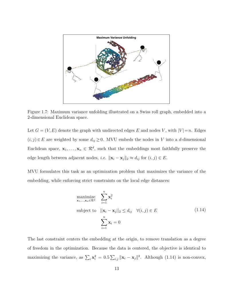
embedding. Figure 1.7 illustrates a 3-dimensional Swiss roll graph being embedded into a

2-dimensional embeddings using MVU. We mainly introduce MVU from the perspective of

graph embedding in which a graph to embed is given in advance.

12

Maximum Variance Unfolding

Figure 1.7: Maximum variance unfolding illustrated on a Swiss roll graph, embedded into a2-dimensional Euclidean space.

Let G = (V,E) denote the graph with undirected edges E and nodes V , with |V |=n. Edges

(i, j)∈E are weighted by some dij ≥ 0. MVU embeds the nodes in V into a d-dimensional

Euclidean space, x1, . . . ,xn ∈ Rd, such that the embeddings most faithfully preserve the

edge length between adjacent nodes, i.e. ‖xi − xj‖2 ≈ dij for (i, j) ∈ E.

MVU formulates this task as an optimization problem that maximizes the variance of the

embedding, while enforcing strict constraints on the local edge distances:

maximizex1,...,xn∈Rd

n∑i=1

x2i

subject to ||xi − xj||2 ≤ dij ∀(i, j) ∈ En∑i=1

xi = 0

(1.14)

The last constraint centers the embedding at the origin, to remove translation as a degree

of freedom in the optimization. Because the data is centered, the objective is identical to

maximizing the variance, as∑

i x2i = 0.5

∑i,j ‖xi − xj‖2. Although (1.14) is non-convex,

13

Weinberger and Saul [146] show that with a rank relaxation, x∈Rn, this problem can be

rephrased as a convex semi-definite program by optimizing over the inner-product matrix

K, with kij = x>i xj:

maximizeK

trace(K)

subject to kii − 2kij + kjj ≤ d2ij ∀(i, j) ∈ E∑i,j

kij = 0

K � 0.

(1.15)

The final constraint K � 0 ensures positive semi-definiteness and guarantees that K can

be decomposed into vectors x1, . . . ,xn with a straight-forward eigenvector decomposition.

To ensure strictly r−dimensional output, the final embedding is projected into Rd with

principal component analysis (PCA). (This is identical to composing the vectors xi out of

the r leading eigenvectors of K.) The time-complexity of MVU is O(n3 + c3) (where c is the

number of constraints in the optimization problem), which makes it prohibitive for larger

data sets.

1.4 Motivations

Over the past few decades, huge efforts have been made towards making machine learning

models more efficient and accurate. However, people have not been aware of the growing

memory and storage consumption by machine learning until recently when a salient shift

toward mobile and embedded devices requires not only superior accuracy but also compact-

ness of the models. Among many subfields of machine learning and artificial intelligence, we

14

observe that techniques leading to large model size often come from the following two areas:

memory-based learning (a.k.a instance-based learning) and deep learning.

1. memory-based Learning. Many models using memory-based learning are essentially

lazy learning in which the prediction of a model is based on pre-stored instances in the

training set. The most commonly seen example is Support Vector Machines (SVM)

with kernels. SVM requires storing the support vectors in the model file as they are

needed for out-of-sample prediction. For datasets with large training instances, the

number of support vectors could be many, which poses a great challenge for memory

saving. The issue of memory consumption doesn’t solely exist for pure instance-based

learning, but also in its recent application on A∗ search. A good heuristic is key to the

efficiency and optimality of a heuristic search. The “perfect” heuristic is no doubt the

pair-wise distance between any two states, which is prohibitively expensive to store in

memory when there are many states in the graph. A good marriage between tradi-

tional heuristic search and graph embedding addresses this problem by compressing

this “perfect” heuristic with the MVU embedding described in Section 1.3. It maps

an AI state graph to a Euclidean space where the heuristics between any two states is

measured by their Euclidean distance [110].

2. Deep Learning. In the past decade deep neural networks have set new perfor-

mance standards in many high-impact applications. These include object classifica-

tion [72, 124], speech recognition [63], image caption generation [141, 68] and domain

adaptation [52]. As data sets increase in size, so do the number of parameters in these

neural networks in order to absorb the enormous amount of supervision [32]. Increas-

ingly, these networks are trained on industrial-sized clusters [76] or high-performance

graphics processing units (GPUs) [32]. Simultaneously, there has been a second trend

15

as applications of machine learning have shifted toward mobile and embedded devices.

As examples, modern smart phones are increasingly operated through speech recogni-

tion [123], robots and self-driving cars perform object recognition in real time [98], and

medical devices collect and analyze patient data [82]. In contrast to GPUs or comput-

ing clusters, these devices are designed for low power consumption and long battery

life.Most importantly, they typically have small working memory. For example, even

the top-of-the-line iPhone 6 only features a mere 1GB of RAM3, let alone other current

wearable devices.

As a matter of fact, mobile and embedded devices fall short of memory capacity. The growing

size of machine learning models creates a dilemma when they are to be deployed on mobile

devices. While it is possible to train models offline on industrial-sized clusters (server-side),

the sheer size of the most effective models would exceed the available memory, making it

prohibitive to perform testing on-device. In speech recognition, one common cure is to

transmit processed voice recordings to a computation center, where the voice recognition is

performed server-side [29]. This approach is problematic, as it only works when sufficient

bandwidth is available and incurs artificial delays through network traffic [70]. One solution

is to train small models for the on-device usage; however, these tend to significantly impact

accuracy [29], leading to customer frustration.

With scalability and, most importantly, compactness in mind, this dissertation describes a

series of work addressing two main problems: 1) Scalability issue of MVU which is key to

the compactness of the memory-based heuristics. 2) Redundancy in neural networks which

poses a great challenge for both compactness and efficiency of deep learning.

3http://en.wikipedia.org/wiki/IPhone_6

16

1.4.1 Scalability of MVU

Euclidean heuristic (EH) [110] has been proposed for A* search. EH exploits manifold learn-

ing methods, in particular MVU, to construct an embedding for each state in the state space

graph, and derives an admissible heuristic distance between two states from the Euclidean

distance between their respective embedded points. EH has shown good performance and

memory efficiency in comparison to other existing heuristics such as differential heuristics.

However, the training of MVU is slow, which greatly limits the scale of AI problems EH can

be applied to.

To address the scalability issue of MVU, we introduce MVC (Maximum Variance Correc-

tion) [20], which finds large-scale feasible solutions to MVU by post-processing embeddings

from any manifold learning algorithm. It increases the scale of MVU embeddings by several

orders of magnitude and is naturally parallel. We demonstrate unprecedented scalability on

MVU training and un-matched reductions in search time across several non-trivial A∗ bench-

mark search problems. Moreover, this work bridges the gap between the manifold learning

literature and the traditional heuristic search, which have been regarded as two fundamen-

tally different fields, leading to cross-fertilization of both fields. It is worth mentioning that

we have another work [25] that solves general submodular maximization leveraging heuristic

search, which serves as a concrete example of heuristic search helping machine learning.

We further propose a number of techniques [23, 86] that can significantly improve the quality

of EH. We propose a goal-oriented manifold learning scheme that optimizes the Euclidean

distance to goals in the embedding while maintaining admissibility and consistency. We

also propose a state heuristic enhancement technique to reduce the gap between heuristic

and true distances. The enhanced heuristic is admissible but no longer consistent. We

17

then employ a modified search algorithm, known as B′ algorithm, that achieves optimality

with inconsistent heuristics using consistency check and propagation. We demonstrate the

effectiveness of the above techniques and report superior reduction in search costs across

several non-trivial benchmark search problems.

1.4.2 Redundancy in neural networks

As deep nets are increasingly used in applications suited for mobile devices, a fundamental

dilemma becomes apparent: the trend in deep learning is to grow models to “absorb” ever-

increasing data set sizes; however mobile devices are designed with very little memory and

cannot store such large models. In the meantime, accumulated evidence suggests [39, 3, 78,

34, 57] that much of the information stored within network weights may be redundant.

We present a novel network architecture, HashedNets [26], that exploits inherent redundancy

in neural networks to achieve drastic reductions in model sizes. HashedNets use a low-cost

hash function to randomly group connection weights into hash buckets, and all connections

within the same hash bucket share a single parameter value. These parameters are tuned to

adjust to the HashedNets weight sharing architecture with standard backpropagation during

training. Our hashing procedure introduces no additional memory overhead, and we demon-

strate on several benchmark data sets that HashedNets shrink the storage requirements of

neural networks substantially while mostly preserving generalization performance.

We further extend the hashing technique to convolutional neural networks (CNN) [27], which

are increasingly used in many areas of computer vision. We present a novel network archi-

tecture, Frequency-Sensitive Hashed Nets (FreshNets), which exploits inherent redundancy

in both convolutional layers and fully-connected layers of a deep learning model, leading to

18

dramatic savings in storage consumption. Based on the key observation that the weights of

learned convolutional filters are typically smooth and low-frequency, we first convert filter

weights to the frequency domain with a discrete cosine transform (DCT) and use a low-cost

hash function to randomly group frequency parameters into hash buckets. All parameters

assigned the same hash bucket share a single value learned with standard back-propagation.

To further reduce model size we allocate fewer hash buckets to high-frequency components,

which are generally less important. We evaluate FreshNets on eight data sets, and show that

it leads to drastically better compressed performance than several relevant baselines.

Compared to its success in AI applications such as computer vision and speech recognition,

neural networks seem not graining as much popularity as it should be in traditional data

mining tasks. For these tasks, neural networks fall short of the following aspects: 1) the

presence of categorical features can pose problems because neural networks only take nu-

merical features inherently. 2) the interpretability of neural networks leaves something to

be desired because it is a big hassle to extract knowledge from neural networks. Inspired

by word embedding, we advocate a compellingly simple, yet effective neural network archi-

tecture with category embedding to address these problems. It not only directly handles

both numerical and categorical features, but also (and more importantly) provides visual in-

sights on category similarities. At its core, the model learns a numerical embedding for each

category of a categorical feature, based on which we can visualize all categories in the em-

bedding space and extract knowledge of similarity between categories. With the embedding,

similar categories are mapped to nearby regions. In addition, we show that the category

embedding can be seen as a matrix factorization of the weight matrix associated with the

one-hot encoding, leading to great savings in memory consumption. We conduct compre-

hensive empirical evaluation which showcases the efficacy and practicality of our approach,

and provides surprisingly good visualization and clustering for categorical features.

19

Chapter 2

Compressing Heuristics with Graph

Embedding

Graph embedding and manifold learning have become a strong sub-field of machine learning

with many mature algorithms [121, 81], often accompanied by large scale extensions [108,

129, 147] and thorough theoretical analysis [42, 104]. Until recently, this success story was

not matched by comparably strong applications [8]. Rayner et al. [110] propose Euclidean

Heuristic (EH) which uses the Euclidean embedding of a search space graph as a heuristic

for A∗ search [119]. The graph-distance between two states is approximated by the Euclidean

distance between their respective embedded points.

Exact A∗ search with informed heuristics is an application of great importance in many areas

of real life. For example, GPS navigation systems need to find the shortest path between two

locations efficiently and repeatedly (e.g. each time a new traffic update has been received,

or when the driver makes a wrong turn). As the processor capabilities of these devices and

the patience of the users are both limited, the quality of the search heuristic is of great

importance. This importance only increases as increasingly low powered embedded devices

(e.g. smart-phones) are equipped with similar capabilities.

20

A perfect heuristic is no doubt the pair-wise shortest-path distance between any two states

in the state graph, which is prohibitively expensive to store in memory. In this chapter, we

study how to use graph embedding to compress this perfect heuristic and how to scale it

up. In particular, we introduce EH in Section 2.1 which at its core is a MVU embedding

described in Chapter 1. We then present a novel embedding algorithm, maximum variance

correction (MVC) [20], to speed up MVU by several order of magnitude. We further extend

the EH to Goal-Oriented Euclidean Heuristics (GOEH) [23] in Section 2.2 to improve the

performance of heuristic search.

2.1 Maximum variance correction for speeding up MVU

2.1.1 Introduction

For an embedding to be aA∗ heuristic, it must satisfy two properties: 1. admissible (distances

are never overestimated), 2. consistent (a triangular inequality like property is preserved).

To be maximally effective, a heuristic should have a minimal gap between its estimate and

the true distance—i.e. all pair-wise distances should be maximized under the admissibil-

ity and consistency constraints. In the applications highlighted by Rayner et al. [110], a

heuristic must require small space to be broadcasted to the end-users. The authors show

that the constraints of Maximum Variance Unfolding (MVU) [146]4 guarantee admissibility

and consistency, while the objective maximizes distances and reduces space requirement of

heuristics from O(n2) to O(dn). In other words, the MVU manifold learning algorithm is a

perfect fit to learn Euclidean heuristics for A∗ search.

4Throughout this dissertation we refer to MVU as the formulation with inequality constraints.

21

Unfortunately, it is fair to say that due to its semi-definite programming (SDP) formula-

tion [11], MVU is amongst the least scalable manifold learning algorithms and cannot embed

state spaces beyond 4000 states—severally limiting the usefulness of the proposed heuristic

in practice. Although there have been efforts to increase the scalability of MVU [145, 147],

these lead to approximate solutions which no longer guarantee admissibility or consistency

of heuristics.

In this chapter we propose a novel algorithm, Maximum Variance Correction (MVC), which

improves the scalability of MVU by several orders of magnitude. In a nutshell, MVC post-

processes embeddings from any manifold learning algorithm, to strictly satisfy the MVU

constraints by rearranging embedded points within local patches. Hereby MVC combines the

strict finite-size guarantees of MVU with the large-scale capabilities of alternative algorithms.

Further, it bridges the gap between the rich literature on manifold learning and what we

consider its most promising and high-impact application to date—the use of Euclidean state-

space embeddings as A∗ heuristics.

Our contributions are summarized as follows: 1) We introduce MVC, a fully parallelizable

algorithm that scales up and speeds up MVU by several orders of magnitudes. 2) We provide

a formal proof that any solution of our relaxed problem formulation still satisfies all MVU

constraints. 3) We demonstrate on several A∗ search benchmark problems that the result-

ing heuristics lead to impressive reductions in search-time—even beating the competitive

differential heuristic [102] by a large factor on all data sets.

22

2.1.2 Background and related work

There have been several recent publications that increase the scalability of manifold learning

algorithms. Vasiloglou et al. [140], Weinberger et al. [147], Weinberger and Saul [146] directly

scale up MVU by relaxing its constraints and restricting the solution to the space spanned

by landmark points or the eigenvectors of the graph laplacian matrix. Silva and Tenenbaum

[129], Talwalkar et al. [136] scale up Isomap [137] with Nystrom approximations. Our work is

complementary as we refine these embeddings to meet the MVU constraints while maximizing

the variance of the embedding.

Shaw and Jebara [126] introduce structure preserving embedding, which learns embeddings

that strictly preserve graph properties (such as nearest neighbors). Zhang et al. [159] also

focus on local patches of manifolds, however preserves discriminative ability rather than the

finite-size guarantees of MVU.

From a technical stand-point, the technique used by MVC is probably most similar to Biswas

and Ye [7] which uses a semi-definite program for sensor network embedding. Due to the

nature of their application, they deal with different constraints and objectives.

Graph Embeddings

We have introduced MVU in Chapter 1. In this section, we mainly introduce other graph

embedding algorithms. Let G = (V,E) denote the graph with undirected edges E and nodes

V , with |V |=n. Edges (i, j)∈E are weighted by some dij ≥ 0. Let δij denote the shortest

path distance from node i to j. Manifold learning algorithms embed the nodes in V into a

d-dimensional Euclidean space, x1, . . . ,xn ∈ Rd, such that ‖xi − xj‖2 ≈ δij.

23

Graph Laplacian MVU (gl-MVU), Weinberger and Saul [146], Wu et al. [150], is an ex-

tension of MVU that reduces the size of K by matrix factorization, K = Q>LQ. Here, Q

are the bottom eigenvectors of the Graph Laplacian, also referred to as Laplacian Eigen-

maps [4]. All local distance constraints are removed and instead added as a penalty term

into the objective. The resulting algorithm scales to larger data sets but makes no exact

guarantees about the distance preservations.

Isomap, Tenenbaum et al. [137], preserves the global structure of the graph by directly

preserving the graph distances between all pair-wise nodes:

minx1,...,xn∈Rd

∑i,j

((xi − xj)2 − δ2ij)2. (2.1)

Tenenbaum et al. [137] show that (2.1) can be approximated as an eigenvector decomposition

by applying multi-dimensional scaling (MDS) [73] on the shortest path distances δ(i, j)5.

The landmark extension [129] leads to significant speed-ups with Nystrom approximations

of the graph-distance matrix. For simplicity, we refer to it also as “Isomap” throughout this

dissertation.

Euclidean Heuristic

The A∗ search algorithm finds the shortest path between two nodes in a graph. In the worst

case, the complexity of the algorithm is exponential in the length of the shortest path, but

the search time can be drastically reduced with a good heuristic, which estimates the graph

distance between two nodes. Rayner et al. [110] suggest to use the distance h(i, j)=‖xi−xj‖25Recent studies [88, 89] give efficient implementation for computing all-pair shortest-path distance on

GPUs.

24

of the MVU graph embedding as such a heuristic, which they refer to as Euclidean Heuristic.

A∗ with this heuristic provably converges to the exact solution, as the heuristic is admissible

and consistent. More precisely, for all nodes i, j, k the following holds:

Admissibility: ‖xi − xk‖2 ≤ δik (2.2)

Consistency: ‖xi − xj‖2 ≤ δik + ‖xk − xj‖2 (2.3)

The proof is straight-forward. As the shortest-path between nodes i and j in the embedding

consists of edges which are all underestimated, it must be underestimated itself and so is

‖xi − xj‖2 (which implies admissibility). Consistency follows from the triangular inequality

in combination with(2.2).

The closer the gap in the admissibility inequality (2.2), the better is the search heuristic. The

perfect heuristic would be the actual shortest path, h(i, j) = δij (with which A∗ could find

the exact solution in linear time with respect to the length of the shortest path). The MVU

objective maximizes all pairwise distances, and therefore minimizes exactly the gap in (2.2).

Consequently, MVU is the perfect optimization problem to find a Euclidean Heuristic—

however in its original formulation it can only scale to n ≈ 4000. In the following we will

scale up MVU to much larger data sets.

2.1.3 Method

In this section, we introduce our MVC algorithm. Intuitively, MVC combines the scalability

of gl-MVU and Isomap with the strong guarantees of MVU: It uses the former to obtain an

initial embedding of the data and then post-processes it into a local optimum of the MVU

25

optimization. The post-processing only involves re-optimizations of local patches, which is

fast and can be decomposed into independent sub-problems.

Initialization. We obtain an initial embedding x1, . . . , xn of the graph with any (large-

scale) manifold learning algorithm (e.g. Isomap, gl-MVU or Eigenmaps). The resulting

embedding is typically not a feasible solution to the exact MVU problem, because it violates

many distance inequality constraints in (1.14). To make it feasible, we first center it and

then rescale the entire embedding such that all inequalities hold with at least one equality,

xi = α(xi −1

n

n∑i=1

xi), with α=min(i,j)∈E

dij‖xi − xj‖

. (2.4)

After the translation and rescaling in (2.4) we obtain a solution in the feasible set of MVU

embeddings, and therefore also an admissible and consistent Euclidean Heuristic. In practice,

this heuristic is of very limited use because it has a very large admissibility gap (2.2). In

the following sections we explain how to transform the embedding to maximize the MVU

objective, while remaining inside the MVU feasible region.

Local patching

The (convex) MVU optimization is an SDP, which in their general formulation scale cubic in

the input size n. To scale-up the optimization we therefore utilize a specific property of the

MVU constraints: All constraints are strictly local as they only involve directly connected

nodes. This allows us to divide up the graph embedding into local patches and re-optimize

the MVU optimization on each patch individually. This approach has two clear advantages:

the local patches can be made small enough to be re-optimized very quickly and the indi-

vidual patch optimizations are inherently parallelizable—leading to even further speed-ups

26

on modern multi-core computers. A challenge is to ensure that the local optimizations do

not interfere with each other and remain globally feasible.

Graph partitioning. There are several ways to divide the graph G=(V,E) into r mutually

exclusive connected components. We use repeated breadth first search (BFS) [119] because

of its simplicity, fast speed and guarantee that all partitions are connected components.

Specifically, we pick a node i uniformly at random and apply BFS to identify the m closest

nodes according to graph distance, that are not already assigned to patches. These nodes

form a new patch Gp = (Vp, Ep). The partitioning is continued until all nodes in V are

assigned to exactly one partition, resulting in approximately r=dn/me patches.6 The final

partitioning satisfies V = V1 ∪ . . . ∪ Vr and Vp ∩ Vq={} for all p, q.

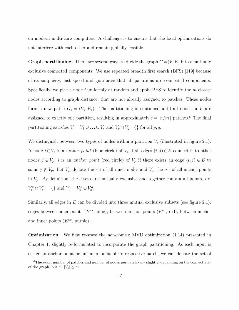
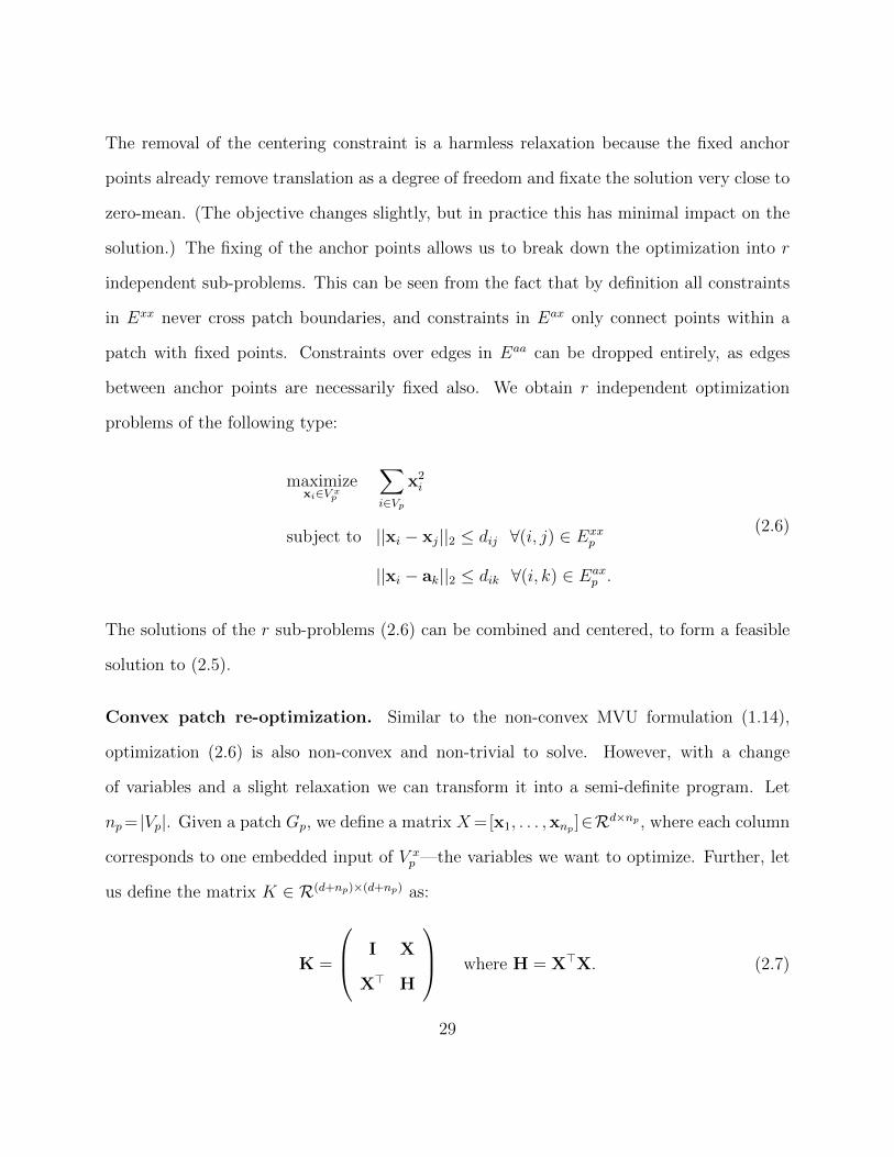
We distinguish between two types of nodes within a partition Vp (illustrated in figure 2.1).

A node i∈ Vp is an inner point (blue circle) of Vp if all edges (i, j)∈E connect it to other

nodes j ∈ Vp; i is an anchor point (red circle) of Vp if there exists an edge (i, j) ∈ E to

some j /∈ Vp. Let V xp denote the set of all inner nodes and V a

p the set of all anchor points

in Vp. By definition, these sets are mutually exclusive and together contain all points, i.e.

V xp ∩ V a

p = {} and Vp = V xp ∪ V a

p .

Similarly, all edges in E can be divided into three mutual exclusive subsets (see figure 2.1):

edges between inner points (Exx, blue); between anchor points (Eaa, red); between anchor

and inner points (Eax, purple).

Optimization. We first re-state the non-convex MVU optimization (1.14) presented in

Chapter 1, slightly re-formulated to incorporate the graph partitioning. As each input is

either an anchor point or an inner point of its respective patch, we can denote the set of

6The exact number of patches and number of nodes per patch vary slightly, depending on the connectivityof the graph, but all |Vp| ≤ m.

27

inner pointanchor pointExx

Eax

Eaa

Gp

xi

xj

ak

Figure 2.1: Drawing of a patch with inner and anchor points.

all inner points as V x =⋃p V

xp and the set of all anchor points as V a =

⋃p V

ap . If we re-

order the summations and constraints by these sets, we can re-phrase the non-convex MVU

optimization (1.14) as

maximizexi,ak

∑i∈V x

x2i +

∑k∈V a

a2k

subject to ||xi − xj||2 ≤ dij ∀(i, j) ∈ Exx

||xi − ak||2 ≤ dik ∀(i, k) ∈ Eax

||ai − aj||2 ≤ dij ∀(i, j) ∈ Eaa∑ai∈V a

ai +∑

xi∈V x

xi = 0.

(2.5)

For clarity, we denote all anchor points as ai’s and inner points as xj’s and with a slight

abuse of notation write ai ∈ V a.

Optimization by patches. The optimization (2.5) is identical to the non-convex MVU

formulation (1.14) and just as hard to solve. To reduce the computational complexity we

make two changes: we remove the centering constraint and fix the anchor points in place.

28

The removal of the centering constraint is a harmless relaxation because the fixed anchor

points already remove translation as a degree of freedom and fixate the solution very close to

zero-mean. (The objective changes slightly, but in practice this has minimal impact on the

solution.) The fixing of the anchor points allows us to break down the optimization into r

independent sub-problems. This can be seen from the fact that by definition all constraints

in Exx never cross patch boundaries, and constraints in Eax only connect points within a

patch with fixed points. Constraints over edges in Eaa can be dropped entirely, as edges

between anchor points are necessarily fixed also. We obtain r independent optimization

problems of the following type:

maximizexi∈V x

p

∑i∈Vp

x2i

subject to ||xi − xj||2 ≤ dij ∀(i, j) ∈ Exxp

||xi − ak||2 ≤ dik ∀(i, k) ∈ Eaxp .

(2.6)

The solutions of the r sub-problems (2.6) can be combined and centered, to form a feasible

solution to (2.5).

Convex patch re-optimization. Similar to the non-convex MVU formulation (1.14),

optimization (2.6) is also non-convex and non-trivial to solve. However, with a change

of variables and a slight relaxation we can transform it into a semi-definite program. Let

np= |Vp|. Given a patch Gp, we define a matrix X=[x1, . . . ,xnp ]∈Rd×np , where each column

corresponds to one embedded input of V xp —the variables we want to optimize. Further, let

us define the matrix K ∈ R(d+np)×(d+np) as:

K =

I X

X> H

where H = X>X. (2.7)

29

The vector ei,j ∈ Rnp is all-zero except the ith element is 1 and the jth element is −1. The

vector ei is all-zero except the ith element is −1. With this notation, we obtain

(0; eij)>K(0; eij) = ‖xi − xj‖22

(ak; ei)>K(ak; ei) = ‖xi − ak‖22,

(2.8)

where (0; eij) ∈ R(d+np) denotes the vector eij padded with zeros on top and (ak; ei) ∈

R(d+np) the concatenation of ak and ei.

Through (2.8), all constraints in (2.6) can be re-formulated as a linear form of K (after

squaring). The objective reduces to trace(H) =∑np

i=1 x2i . The resulting optimization prob-

lem becomes:

maxX,H

trace(H)

s.t. (0; eij)>K(0; eij) ≤ d2ij ∀(i, j) ∈ Exx

p

(ak; ei)>K(ak; ei) ≤ d2ik ∀(i, k) ∈ Eax

p

H = X>X

K =

I X

X> H

.

(2.9)

The constraint H = X>X fixes the rank of H and is not convex. To mitigate, we relax it

into H � X>X. In the following section we prove that this weaker constraint is sufficient to

obtain MVU-feasible solutions. The Schur Complement Lemma [11] states that H � X>X

30

Algorithm 1 MVC (V,E)1: compute initial solution X with gl-MVU or Isomap2: center and rescale X according to (2.4)3: repeat4: identify r random sub-graphs (V1, E1), . . . , (Vr, Er)5: parfor p=1 to r do6: solve (2.10) for (Vp, Ep) to obtain Xp

7: end parfor8: concatenate all Xp into X and center.9: until variance of embedding X has converged.

10: return X

if and only if K � 0, which we enforce as an additional constraint:

maxX,H

trace(H)

s.t. (0; eij)>K(0; eij) ≤ d2ij ∀(i, j) ∈ Exx

p

(ak; ei)>K(ak; ei) ≤ d2ik ∀(i, k) ∈ Eax

p

K =

I X

X> H

� 0.

(2.10)

The optimization (2.10) is convex and scales O((np + d)3). It monotonically increases the

objective in (2.5) and converges to a fixed point. For a maximum patch-size m, i.e. np≤m

for all p, each iteration of MVC scales linearly with respect to n, with complexity O(d nme(m+

d)3). As the choice of m is independent of n, it can be fixed to a medium-sized value e.g.

m≈500 for maximum efficiency. The r≈d nme sub-problems are completely independent and

can be solved in parallel, leading to almost perfect parallel speed-up on computing clusters.

The same methodology also applies to 3D modeling [164, 163, 161, 162]. Algorithm 1 states

MVC in pseudo-code.

31

MVU feasibility

We prove that the MVC algorithm returns a feasible MVU solution and consequently gives

rise to a well defined Euclidean Heuristic. First we need to show that the relaxation from

H = X>X to H � X>X does not cause any constraint violations.

Lemma 1. The solution X of (2.10) satisfies all constraints in (2.6).

Proof. We first focus on constraints on (i, j)∈Exxp . The first constraint in (2.10) guarantees

Hii − 2Hij + Hjj ≤ d2ij. (2.11)

The last constraint of (2.10) and the Schur Complement Lemma enforce that H−X>X � 0.

Thus,

e>ij(H−X>X)eij ≥ 0

⇔ e>ij(X>X)eij ≤ e>ijHeij (2.12)

⇔ x2i − 2x>i xj + x2

j ≤ Hii − 2Hij + Hjj

⇔ ‖xi − xj‖22 ≤ Hii − 2Hij + Hjj. (2.13)

The first result follows from the combination of (2.11) and (2.13). Concerning constraints

(i, j)∈Eaxp , the second constraint in (2.10) guarantees that

a2k − 2a>k xi + Hii ≤ d2ik. (2.14)

32

With a similar reasoning as for (2.12) we obtain e>i (X>X)ei ≤ e>i Hei and therefore x2i ≤ Hii.

Combining this inequality with (2.14) leads to the result:

‖ak − xi‖22 ≤ a2k − 2akxi + Hii ≤ d2ik. �

Theorem 1. The embedding obtained with the MVC Algorithm 1 is in the feasible set of

(1.14).

Proof. We apply an inductive argument. The initial solution after centering and re-scaling

according to (2.4) is MVU feasible by construction. By Lemma 1, the solution of (2.10)

for each patch satisfies all constraints in Exxp and Eax

p in (2.6). As each distance constraint

in (2.5) is associated with exactly one patch, all its constraints in Exx and Eax are satis-

fied. Constraints in Eaa are fixed and satisfied by the induction hypothesis. Centering X

satisfies the last constraint in (2.5) and leaves all distance constraints unaffected. As (2.5)

is equivalent to (1.14), we obtain an MVU feasible solution at the end of each iteration in

Algorithm 1, which concludes the proof. �

2.1.4 Experimental results

We evaluate our algorithm on a real world shortest path application data set and on two

well-known benchmark AI problems.

Game Maps is a real world map dataset with 3,155 states from the international success

multi-player game Biowares Dragon Age: OriginsTM .7 A game map is a maze that consists

of empty spaces (states) and obstacles. Cardinal moves take unit costs while diagonal moves

7http://en.wikipedia.org/wiki/Dragon_Age:_Origins

33

0

0.05

0.1

0.15

>0.2

0

0.05

0.1

0.15

>0.2

0

0.05

0.1

0.15

>0.2

0

0.05

0.1

0.15

0.2

0

0.05

0.1

0.15

>0.2

0

0.05

0.1

0.15

>0.2

0

0.05

0.1

0.15

>0.2Isomap: var=5456 MVC: iter=1, var=8994

MVC: iter=16, var=11422

MVC: iter=2, var=10274 MVC: iter=4, var=11046

MVC: iter=8, var=11396 MVC: iter=46, var=11435

0

0.05

0.1

0.15

>0.2MVU: var=11435

>0.20

0.15

0.10

0.05

0

ξ

Figure 2.2: Visualization of several MVC iterations on the 5-puzzle data set (m = 30). Theedges are colored proportional to their relative admissibility gap ξ, as defined in (2.15). Thetop left image shows the (rescaled) Isomap initialization. The successive graphs show thatMVC decreases the edge admissibility gaps and increases the variance with each iteration(indicated in the title of each subplot) until it converges to the same variance as the MVUsolution (bottom right).

cost 1.5. The search problem is to find an optimal path between a given start and goal state,

while avoiding all obstacles. Although not large-scale, this data set is a great example for

an application where the search heuristic is of extraordinary importance. Speedy solvers are

essential to reduce upkeep costs and to ensure a positive user experience. In the game, many

player and non-player characters interact and search problems have to be solved frequently as

agents move. The shortest path solutions cannot be cached as the map changes dynamically

with player actions.

M-Puzzle Problem [67] is a NP-hard sliding puzzle, often used as a benchmark problem

for search algorithms/heuristics. It consists of a frame of M square tiles and one tile missing.

All tiles are numbered and a state constitutes any order from which a path to the unique

state with sorted (increasing) tiles exists. An action is to move a cardinal neighbor tile of

34

Table 2.1: Relative A∗ search speedup over the differential heuristic (in expanded nodes)and embedding variance (×105).

game map 6-blocksworld 7-puzzle 7-blocksworld 8-puzzle

Method speedup var speedup var speedup var speedup var speedup var

Diff. Heuristic 1 N/A 1 N/A 1 N/A 1 N/A 1 N/A

Eigenmap 0.32 0.88 0.66 0.058 0.81 3.52 0.61 0.50 0.76 13.47Isomap 0.50 12.13 0.61 0.046 0.84 3.73 0.65 0.46 0.67 10.62MVU 1.12 37.27 1.23 0.154 N/A N/A N/A N/A N/A N/Agl-MVU 0.41 7.54 1.18 0.138 1.14 6.66 1.05 1.20 0.88 17.79

MVC-10 (eigenmap) 0.88 31.31 1.49 0.22 1.41 9.59 1.33 1.88 1.47 43.48MVC-10 (isomap) 1.09 36.96 1.56 0.22 1.43 9.62 1.25 1.71 1.45 43.08MVC-10 (gl-mvu) 0.90 32.98 1.96 0.27 1.45 9.82 1.67 2.27 1.52 45.75

MVC (eigenmap) 1.06 35.92 2.08 0.29 1.45 9.86 2.17 2.93 1.54 46.52MVC (isomap) 1.12 37.22 2.22 0.30 1.47 9.85 2.22 2.95 1.54 46.58MVC (gl-mvu) 1.11 36.47 2.27 0.30 1.45 9.86 2.22 2.95 1.61 49.06

the empty space into the empty space. The task is to find a shortest action sequence from

a pre-defined start to a goal state. We evaluate our algorithm on the 5- (for visualization),

7- and 8-puzzle problem (3×2, 4×2 and 3×3 frames), which contain 360, 20160 and 181440

states respectively.

Blocks World [55] is a NP-hard problem with the goal to build several pre-defined stacks

out of a set of numbered blocks. Blocks can be placed on the top of others or on the ground.

Any block that is currently under another block cannot be moved. The goal is to find a

minimum action sequence from a start state to a goal state. We evaluate our algorithm on

block world problems with 6 blocks (4,051 states) and 7 blocks (37,633 states), respectively.

Problem characteristics. The three types of problems not only feature different sized state

spaces but also have different state space characteristics. Game maps has random obstacles

that prevents movement for some state pairs, and thus has an irregular state space. The

puzzle problems have a more regular search space (which lie on the surface of a sphere, see

figure 2.2) with stable out-degree for each state. The state space of the blocksworld problems

35

is also regular (it lies inside a sphere); however, the out-degree varies largely across states.

For example, in 7-blocks, the state in which every block is placed on the ground has 42 edges,

while the state in which all blocks are stacked in a single column has only 1 edge. We set

dij =1 for all edges in blocksworld and M -puzzle problems.

Experimental setting. Besides MVC, we evaluate four graph embedding algorithms:

MVU [146], Isomap [137], (Laplacian) Eigenmap [4] and gl-MVU [150]. The last three

are used as initializations for MVC. Following Rayner et al. 110, the embedding dimension

is d = 3 for all experiments. For gl-MVU, we set the dimension of graph Laplacian to be 40.

For datasets of size greater than 10K, we set 10K landmarks for Isomap. For MVC we use

a patch-size of m=500 throughout (for which problem (2.10) can be solved in less than 20s

on our lab desktops).

Visualization of MVC iterations (m = 30). Figure 2.2 visualizes successive iterations

of the d= 3 dimensional MVC embedding of the 5−puzzle problem. All edges are colored

proportionally to their relative admissibility gap,

ξij =dij − ||xi − xj||||xi − xj||

. (2.15)

The plot in the top left shows the original Isomap initialization after re-scaling, as defined

in (2.4). The plot in the bottom right shows the actual MVU embedding from (1.15)—

which can be computed precisely because of the small problem size. Intermediate plots

show the embeddings after several iterations of MVC. Two trends can be observed: 1. the

admissibility gap decreases with MVC (all edges are blue in the final embedding) and 2. the

variance∑

i x2i of the embedding, i.e. the MVU objective, increases monotonically. The final

embedding has the same variance as the actual MVU embedding. The figure also shows that

the 5−puzzle state space lies on a sphere, which is a beautiful example that visualization

36

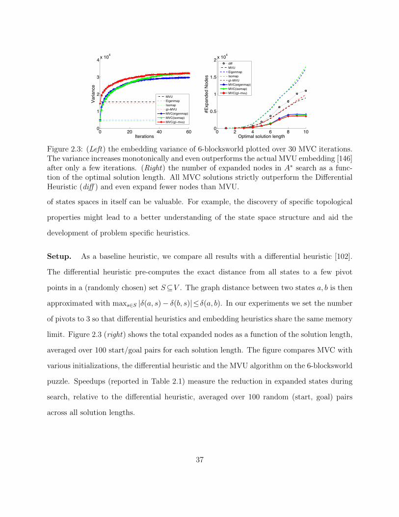
0 20 40 600

1

2

3

4 x 104

Iterations

Varia

nce

MVUEigenmapIsomapgl MVUMVC(eigenmap)MVC(isomap)MVC(gl mvu)

0 2 4 6 8 100

0.5

1

1.5

2 x 104

Optimal solution length

#Exp

ande

d No

des

diffMVUEigenmapIsomapgl MVUMVC(eigenmap)MVC(isomap)MVC(gl mvu)

Figure 2.3: (Left) the embedding variance of 6-blocksworld plotted over 30 MVC iterations.The variance increases monotonically and even outperforms the actual MVU embedding [146]after only a few iterations. (Right) the number of expanded nodes in A∗ search as a func-tion of the optimal solution length. All MVC solutions strictly outperform the DifferentialHeuristic (diff ) and even expand fewer nodes than MVU.

of states spaces in itself can be valuable. For example, the discovery of specific topological

properties might lead to a better understanding of the state space structure and aid the

development of problem specific heuristics.

Setup. As a baseline heuristic, we compare all results with a differential heuristic [102].

The differential heuristic pre-computes the exact distance from all states to a few pivot

points in a (randomly chosen) set S⊆V . The graph distance between two states a, b is then

approximated with maxs∈S |δ(a, s)− δ(b, s)|≤δ(a, b). In our experiments we set the number

of pivots to 3 so that differential heuristics and embedding heuristics share the same memory

limit. Figure 2.3 (right) shows the total expanded nodes as a function of the solution length,

averaged over 100 start/goal pairs for each solution length. The figure compares MVC with

various initializations, the differential heuristic and the MVU algorithm on the 6-blocksworld

puzzle. Speedups (reported in Table 2.1) measure the reduction in expanded states during

search, relative to the differential heuristic, averaged over 100 random (start, goal) pairs

across all solution lengths.

37

Table 2.2: Training time for MVU [145] and MVC, reported after initialization, the first 10iterations (MVC-10), and after convergence.

Method game 6-block 7-puzz 7-block 8-puzz|V | 3,155 4,051 20,160 37,633 181,440MVU 3h 10h N/A N/A N/AEigenmap 1s 1s 4s 2m 7mIsomap 14s 57s 3m 4m 32mgl-MVU 2m 1m 1m 8m 15mMVC-10 (eig) 20m 2m 14m 9m 2hMVC-10 (iso) 15m 3m 20m 11m 3hMVC-10 (glm) 21m 3m 18m 14m 3hMVC (eig) 36m 9m 72m 53m 6hMVC (iso) 17m 8m 56m 51m 7hMVC (glm) 34m 5m 26m 33m 7h

Comprehensive evaluation. Table 2.1 shows the A∗ search performances of Euclidean

heuristics obtained by the MVC initializations, MVC after only 10 iterations (MVC-10)

and after convergence (bottom section). Table 2.1 also shows the MVU objective/variance,∑x∈V x2

i , of each embedding. Several trends can be observed: 1. MVC performs best when

initialized with gl-MVU—this is not surprising as gl-MVU has a similar objective and is

likely to lead to better initializations; 2. all MVC embeddings lead to drastic speedups over

the differential heuristics; 3. the variance is highly correlated with speedup—supporting

Rayner et al. [110] that the MVU objective is well suited to learn Euclidean heuristics; 4.

even MVC after only 10 iterations already outperforms the differential heuristic on almost

all data sets. The consistency of the speedups and their unusually high factors (up to 2.22)

show great promise for MVC as an embedding algorithm for Euclidean heuristics.

Exceeding MVU. On the 6-blocksworld data set in table 2.1, the variance of MVC actu-

ally exceeds that of MVU. In other words, the MVC algorithm finds a better solution for

(1.14). This phenomenon can be explained by the fact that the convex MVU problem (1.15)

38

presented in Chapter 1 is rank-relaxed and the final embedding is obtained after projection

into a d= 3 dimensional sub-space. As MVC performs its optimization directly in this d-

dimensional sub-space, it can find a better rank-constrained solution. This effect is further

illustrated in Figure 2.3 (left), which shows the monotonic increase of the embedding vari-

ance as a function of the MVC iterations (on 6-blocksworld). After only a few iterations, all

three MVC runs exceeds the MVU solution. A similar effect is utilized by Shaw and Jebara

[125], who optimize MVU in lower dimensional spaces directly (but cannot scale to large data

sets). Figure 2.3 (left) also illustrates the importance of initialization: MVC initialized with

Isomap and gl-mvu converge to the same (possibly globally optimal) solution, whereas the

run with Laplacian Eigenmaps initialization is stuck in a sub-optimal solution. Our findings

are highly encouraging and show that we might not only approximate MVU effectively on

very large data sets, but actually outperform it if the intrinsic dimensionality of the data is

higher than the desired embedding dimensionality d.

Embedding time. Table 2.2 shows the training time required for the convex MVU algo-

rithm (1.15), three MVC initializations (Eigenmap, Isomap, gl-MVU), the time for 10 MVC

iterations and the time until MVC converges, across all five data sets. Note that for real

deployment, such as GPS systems, MVC only needs to be run once to obtain the embedding.

The online calculations of Euclidean heuristics are very fast. All embeddings were computed

on an off-the-shelve desktop with two 8-core Intel(R) Xeon(R) processors of 2.67 GHz and

128GB of RAM. Our MVC implementation is in MATLABTM and uses CSDP [9] as the

SDP solver. We parallelize each run of MVC on eight cores. All three initializations require

roughly similar time (although Laplacian Eigenmaps is the fastest on all data sets), which

is only a small part of the overall optimization. Whereas MVU requires 10 hours for graphs

with |V |=4051 (and cannot be executed on larger problems), we can find a superior solution

39

to the same problem in 5 minutes and are able to run MVC on 45× larger problems in only

7 hours.

2.1.5 Conclusion

In this chapter, we have presented MVC, an iterative algorithm to transform graph embed-

dings into MVU feasible solution. On several small-sized problems where MVU can finish,

we show that MVC gives comparable or even better solutions than MVU. We apply MVU

on data sets of unprecedented sizes (n= 180, 000) and, because of linear scalability, expect

future (parallel) implementations to scale to graphs with millions of nodes. By satisfying all

MVU constraints, MVC embeddings are provably well-defined Euclidean heuristics for A∗

search and unleash an exciting new area of applications to all of manifold learning. We hope

it will fuel new research directions in both fields.

2.2 Goal-oriented Euclidean heuristics - a refined Eu-

clidean heuristic

2.2.1 Introduction

With the development of MVC described in Section 2.1, EH becomes an attractive and

scalable choice for computing heuristics. However, its potential is yet to be fully explored.

The objective of MVU/MVC minimizes the sum of the distance gaps between all pairs of

states, while A∗ search is guided only by the heuristic distance to the goal state. In many

applications, possible (or likely) goal states form a small subset of the overall state space.

40

For example, GPS driving assistants are mostly used to find directions to registered street

addresses, which are a tiny fraction of all possible locations on a map. This suggests that

the EH can be further improved by “tightening” the heuristic distances towards likely goal

states.

Moreover, state graphs are typically not isometric to low dimensional Euclidean spaces,

which leads to distance gaps between the EH heuristic and the true distances—in particular,

for states that are far away from each other. We find that it is possible to compactly encode

the information about distance gaps, using only a small amount of memory, and significantly

improve the search performance by correcting heuristic estimates on-the-fly.

Our main contributions include, 1) a goal-oriented graph embedding framework that opti-

mizes the heuristic distance to goals while preserving admissibility and consistency, and 2)

an in-memory enhancement technique that can be used online to speed up search. Since

the enhancement technique generates better heuristics that are admissible but no longer

consistent, we employ the B′ search to make sure that the first solution found is an optimal

one.

2.2.2 Goal-oriented Euclidean heuristic

We make several assumptions about our problem domain: The state-space is represented as

an undirected graph with n nodes, which fits into memory. We are asked to solve search

problems repeatedly, with different starting and goal states. We would like to minimize the

time required for these search problems through better heuristics. The heuristics can be

optimized offline, where computation time is of no particular importance, but the storage

41

required to encode the heuristic must be small (as it might need to be communicated to the

consumers and loaded into memory).

In many A∗ search applications, some states are much more likely to be considered goal

states than others. For example, in video games, certain locations (e.g. treasure targets)

are typical goals that a players might want to move to, whereas most arbitrary positions

in the game space are moved to very infrequently. In the subsequent section we describe a

robot planning domain, where robots can pick up objects from pre-specified source locations

and move them to pre-specified target locations. Here, there exists a strict subset of states

that could potentially become goal states—important information that ideally should be

incorporated into the heuristic design. As a final example, GPS navigation assistants are

typically exclusively used to direct users to registered home addresses—a tiny subset of

all possible locations on the map. Further, a particular user might only traverse between

no more than 100 locations on the world map. It is fair to assume that she might prefer

accelerating the search for these frequent goals, even at the cost that the search for infrequent

goals takes a little longer.

Let G = (V,E) be the state-space graph. For convenience, we assume that there is a subset

of possible goal states VG ⊆ V . When we know a set of possible goals, we can improve EH by

maximizing the distances to the goals. Note that during an A∗ search, only those distances

to the particular goal state will be used as the heuristic function (h), and heuristic distances

between two non-goal states are never used during search. This motivates us to modify the

objective function in the EH/MVU optimization so that it exclusively maximizes distances

to goals. Note that we can still guarantee admissibility and consistency of EH, since we keep

all local constraints.

42

The proposed goal-oriented Euclidean heuristic (GOEH) solves the following:

maximizex1,...,xn∈Rd

∑i=1..n,g∈VG

‖xi − xg‖22

subject to ||xi − xj||2 ≤ dij, ∀(i, j) ∈ En∑i=1

xi = 0

(2.16)

Due to the centering constraint∑n

i=1 xi = 0, the objective in (2.16) can be further reduced

to

maximizex1,...,xn∈Rd

ng∑i=1..n

‖xi‖22 + n∑g∈VG

‖xj‖22, (2.17)

where ng = |VG| is the number of goals.

Following the same rank relaxation as in MVU [146] and considering (2.17), (2.16) can be

rephrased as a convex SDP by optimizing over the inner-product matrix K, with kij = x>i xj:

maximizeK

ngtrace(K) + n∑g∈VG

kgg

subject to kii − 2kij + kjj ≤ d2ij, ∀(i, j) ∈ E∑i,j

kij = 0

K � 0.

(2.18)

The final embedding is projected onto Rd by composing the vectors xi out of the d leading

eigenvectors of K.

Note that a general weighted EH model is already discussed in [110]. However, GOEH makes

the goal-oriented cases explicit.

43

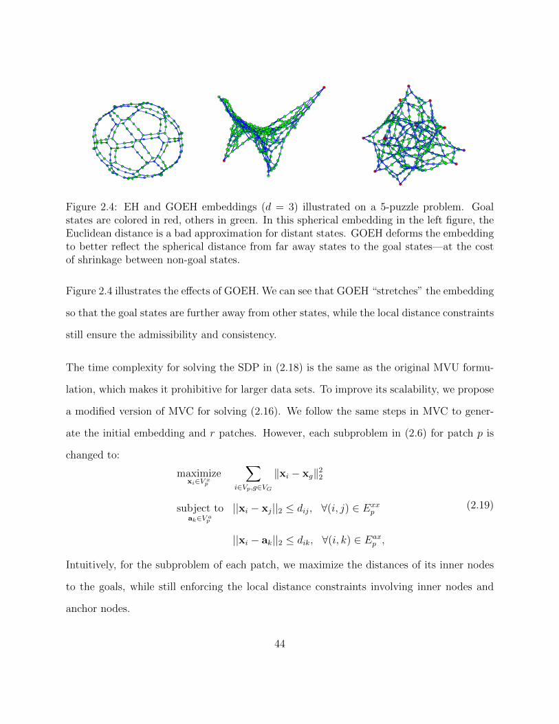
Figure 2.4: EH and GOEH embeddings (d = 3) illustrated on a 5-puzzle problem. Goalstates are colored in red, others in green. In this spherical embedding in the left figure, theEuclidean distance is a bad approximation for distant states. GOEH deforms the embeddingto better reflect the spherical distance from far away states to the goal states—at the costof shrinkage between non-goal states.

Figure 2.4 illustrates the effects of GOEH. We can see that GOEH “stretches” the embedding

so that the goal states are further away from other states, while the local distance constraints

still ensure the admissibility and consistency.

The time complexity for solving the SDP in (2.18) is the same as the original MVU formu-

lation, which makes it prohibitive for larger data sets. To improve its scalability, we propose

a modified version of MVC for solving (2.16). We follow the same steps in MVC to gener-

ate the initial embedding and r patches. However, each subproblem in (2.6) for patch p is

changed to:

maximizexi∈V x

p

∑i∈Vp,g∈VG

‖xi − xg‖22

subject toak∈V a

p

||xi − xj||2 ≤ dij, ∀(i, j) ∈ Exxp

||xi − ak||2 ≤ dik, ∀(i, k) ∈ Eaxp ,

(2.19)

Intuitively, for the subproblem of each patch, we maximize the distances of its inner nodes

to the goals, while still enforcing the local distance constraints involving inner nodes and

anchor nodes.

44

Following a similar approach as in MVC described in Section 2.1, we reformulate (2.19)

as a SDP. Given a patch Gp = (Vp, EP ) with np = |Vp|, we define a design matrix X =

[x1, . . . ,xn] ∈ Rd×np , where each column corresponds to one embedding coordinate of V xp .

Define the matrix K ∈ R(d+np)×(d+np) as:

K =

I X

X> H

where H = X>X. (2.20)

Let the vector ei,j ∈ Rnp be all-zero except the ith element is 1 and the jth element is −1.

Let the vector ei be all-zero except the ith element is −1. With this notation, and the Schur

Complement Lemma [11], we can relax (2.19) into a SDP:

maxX,H

∑i∈V x

p

ngHii −∑g∈V 1

p

2x>g xi +∑g∈V 2

p

(Hgg −Hig)

s.t. (0; eij)

>K(0; eij) ≤ d2ij ∀(i, j) ∈ Exxp

(ak; ei)>K(ak; ei) ≤ d2ik ∀(i, k) ∈ Eax

p

K =

I X

X> H

� 0

(2.21)

where V 1p = VG\V x

p , V 2p = VG ∩ V x

p , Hij are elements in H, xi is the ith column of X, and

xg is the coordinate for node g. The optimization (2.21) is a convex SDP and can be solved

very efficiently for medium sized np. The r sub-problems are completely independent and

can be solved in parallel, leading to almost perfect parallel speed-up on multi-core computers

or clusters. Like MVC, we reiterate solving the r subproblems until convergence.

45

Both the centralized solution in (2.18) and the partitioned solution in (2.21) maintain the

admissibility and consistency of EH, because the constraints are kept the same as in (1.14),

and the proof for admissibility and consistency of EH only relies on these constraints [110].

Proposition 1. Any feasible solution to (2.18) or (2.21) gives admissible and consistent

Euclidean heuristics.

The memory requirement for storing the embedding results x1, . . . ,xn ∈Rd is still O(dn),

which is reasonable since d is often a small constant such as 3 or 4.

2.2.3 State heuristic enhancement

We propose a state heuristic enhancement (SHE) technique to further improve the quality

of GOEH. Since GOEH gives a lower bound of the true distance, we can calculate their gaps

in a preprocessing phase and store the information in the memory to aid the search.

Suppose we are given a state-space graph G = (V,E) and a goal set VG ⊆ V . After we

use GOEH to generate a d-dimensional embedding x1, . . . ,xn∈Rd, for any i = 1, · · · , n, we

store a real number ηi defined as:

ηi = minj∈VG

{dij − ‖xi − xj‖2

}. (2.22)

46

During the search towards any goal g, for any state i, its enhanced heuristic value will be

h(i, g) = ‖xi − xg‖2 + ηi. (2.23)

Intuitively, ηi stores the minimum gap between the EH and true distance from state i to any

goal state in the goal set. During a search, we can add ηi to the Euclidean distance from i

to g in the embedded space. Clearly, we have:

Proposition 2. The heuristic function in (2.23) is admissible.

However, the heuristic in (2.23) is no longer guaranteed to be consistent. A parent node i may

receive a much larger ηi than the ηj received by a child node j, so that h(i, g) > dij +h(j, g),

leading to inconsistency.

As found in [156], inconsistent but admissible heuristics can often be preferable to consistent

heuristics. To ensure optimality of the first solution found, we employ the B′ algorithm

proposed in [93].

Suppose the current expanded node is i, the rules of the B′ algorithm to handle inconsistency

are:

a) For each successor j of i, if h(j, g) < h(i, g)− dij, set h(j, g) = h(i, g)− dij

b) Let j be the successor of i with minimum h(j, g) + dij. If h(i, g) < h(j, g) + dij, set

h(i, g) = h(j, g) + dij

47

2 4 6 8 10 120

2

4

6

8

10

12 x 104

optimal distance

#Exp

ande

d N

odes

Diff (4 pivots)EH (d=4)GOEH (d=4)EH+SHE (d=3)GOEH+SHE (d=3)

10 15 20 25 30 350

1

2

3

4

5 x 104

optimal distance

#Exp

ande

d N

odes

Diff (4 pivots)EH (d=4)GOEH (d=4)EH+SHE (d=3)GOEH+SHE (d=3)

40 50 60 70 800

1

2

3

4 x 104

optimal distance

#Exp

ande

d N

odes

Diff (4 pivots)EH (d=4)GOEH (d=4)EH+SHE (d=3)GOEH+SHE (d=3)

Figure 2.5: The number of expanded nodes in the optimal search as a function of the optimalsolution length. For EH+SHE and GOEH+SHE, B′ search is used and the re-opened nodesare counted as new expansions.

It is shown in [93] that adding those rules to A∗ search makes it optimal even when the

heuristic is inconsistent. They can actually further improve the heuristic since it propagates

improvements on the heuristic values based on consistency constraints. It is also shown that

if the heuristic is consistent, then these rules will never be invoked and the B′ search is exactly

the same as the A∗ search [93]. Experimentally, we found that inconsistency does not occur

often. For many problem instances we tested, the enhanced heuristics are consistent. For

other instances, these B′ rules are invoked for some states to improve their GOEH values.

We note that there is a tradeoff between space complexity and heuristic accuracy. SHE uses

O(n) memory since it stores one real number per state, which adds only 1/d overhead to

the O(dn) space used by EH and GOEH. As we will see, this simple SHE technique can

drastically improve the efficiency of optimal search on every domain we test. Note that EH

cannot utilize dimensions that exceed the intrinsic dimensionality of the state space. This is

in contrast to SHE, which does take advantage of such “extra” dimensions.

48

2.2.4 Experimental results

We evaluate our algorithms on two well-known benchmark AI problems and on a real world

service robot application.

M-Puzzle Problem [67] is a popular benchmark problem for search algorithms. It consists

of a frame of M tiles and one tile missing. All tiles are numbered and a state constitutes

any order of the tiles. An action is to move a cardinal neighbor tile of the empty space into

the empty space. The task is to find a shortest action sequence from a pre-defined start to a

goal state. We evaluate our algorithm on 7- and 8-puzzle problems (4×2 and 3×3 frames),

which contain 20160 and 181440 states, respectively.

Blocks World [55] is a NP-hard problem with the goal to build several given stacks out of

a set of blocks. Blocks can be placed on the top of others or on the ground. Any block that

is currently under another block cannot be moved. We test blocks world problems with 6

blocks (4,051 states) and 7 blocks (37,633 states), respectively.

Home Service Robot is designed to handle daily indoor activities and can interact with

human. In the Home Service Robot Competition at the RoboCup (http://robocup.rwth-

aachen.de/athomewiki/index.php/Main Page), there are a service robot, human, small ob-

jects that can be picked up and moved by the robot, and some big objects that cannot be

moved. A typical task is to ask the robot to pick up a small object and bring it to the

human. In this problem, each state describes different variables, such as the locations of the

robot, human and small objects. There are a lot of intermediate states that the robot never

takes as the goal. The robot can store the precomputed GOEH and SHE information in

memory and use it to solve various daily tasks online.

49

Goal sets. We design three kinds of goal settings for our datasets. For M -puzzles, we

let the goal set include all the states where the first three tiles are blank, tile 1 and tile

2, respectively. In this case, all goal states are distributed uniformly on the surface of the

embedded sphere (see the rightmost subfigure in Figure 2.4). For blocks world problems,

we randomly pick a state and add more states in its vicinity to the goal set. For the home

service robot application, the goal states are built-in goals for completing specific tasks from

the competition. In this way, we evaluate our algorithms on the scenarios of distributed

goals, clustered goals, and real-world goals, leading to a comprehensive assessment.

Experimental setup. We use MVC to learn GOEH and use Isomap [137] to initialize

MVC. For datasets of a size greater than 8K, we set 8K landmarks for Isomap. For MVC we

use a patch size of m=500 throughout (for which problem (2.21) can be solved in less than

20s). Following [110, 20], we choose a small embedding dimensionality for saving memory

space. We set the number of embedding dimensions d = 4 for all experiments, meaning that

each heuristic stores 4n real numbers. Since SHE requires another array of n numbers, the

embedding dimension is set to d = 3 when SHE is used. This gives a fair comparison since

all algorithms use 4n space. In our experiments, all MVC or goal-oriented MVC algorithms

are stopped after a maximum of 50 iterations.

We also test the differential heuristic [102, 134] as a baseline. The differential heuristic

pre-computes the exact distance from all states to a few pivot nodes in a set S ⊆ V . We

implemented the algorithm to select good pivot nodes in [134]. The differential heuristic

between two states a, b is maxs∈S |δ(a, s) − δ(b, s)|≤ δ(a, b). In our experiments, we set the

number of pivot nodes to 4 so that both differential heuristics and Euclidean heuristics have

the same space complexity of 4n.

50

Problem Diff EH GOEH EH+SHE GOEH+SHE

6-block 1.00 3.83 5.77 5.02 6.267-block 1.00 3.02 3.46 15.06 23.30

7-puzzle 1.00 1.40 1.53 2.01 2.088-puzzle 1.00 1.25 1.36 3.20 3.18

robot1 1.00 5.09 14.14 17.12 26.83robot2 1.00 4.63 9.19 14.68 29.28

Table 2.3: Speedup of various methods as compared to the differential heuristic.

Comprehensive evaluation. Figure 2.5 shows the total expanded nodes of three problems

as a function of the optimal solution length, averaged over 500 start/goal pairs for each

solution length. Each goal is randomly chosen from the goal set VG. The figures compare

the performance of the differential heuristic (Diff), EH, GOEH, EH combined with SHE

(EH+SHE), and GOEH+SHE. To quantify the performance improvement, Table 1 shows

the speedup of each method over the differential heuristic, defined as:

Speedup(M) =

∑l

∑500p=1 NumExpand(l,p,Diff)∑

l

∑500p=1 NumExpand(l,p,M)

where NumExpand(l,p,M) is the number of states expanded by algorithm M to solve the pth

start/goal pair under solution length l. From Figure 2 and Table 1, we can see that each

of GOEH and SHE dramatically reduces the number of expanded states. Combining them

gives the most reduction.

Embedding time. Table 2.4 shows the training time for each embedding algorithm. Note

that for real deployment, such as GPS systems, MVC only needs to be run once to obtain

the embedding. This offline computing cost is of no importance – it is the online search

speed that matters to end users. Once such an embedding is loaded into memory, the online

calculation of Euclidean heuristics is very fast. Since we set d = 4 when SHE is not used and

d = 3 when SHE is used, the training times for the MVC optimization in EH and EH+SHE

51

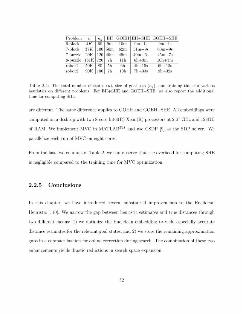
Problem n ng EH GOEH EH+SHE GOEH+SHE

6-block 4K 60 9m 10m 9m+1s 9m+1s7-block 37K 100 56m 62m 51m+9s 60m+9s

7-puzzle 20K 120 40m 49m 40m+6s 45m+7s8-puzzle 181K 720 7h 11h 6h+3m 10h+3m

robot1 50K 80 5h 6h 4h+15s 6h+15srobot2 90K 100 7h 10h 7h+33s 9h+32s

Table 2.4: The total number of states (n), size of goal sets (ng), and training time for variousheuristics on different problems. For EH+SHE and GOEH+SHE, we also report the additionaltime for computing SHE.

are different. The same difference applies to GOEH and GOEH+SHE. All embeddings were

computed on a desktop with two 8-core Intel(R) Xeon(R) processors at 2.67 GHz and 128GB

of RAM. We implement MVC in MATLABTM and use CSDP [9] as the SDP solver. We

parallelize each run of MVC on eight cores.

From the last two columns of Table 2, we can observe that the overhead for computing SHE

is negligible compared to the training time for MVC optimization.

2.2.5 Conclusions

In this chapter, we have introduced several substantial improvements to the Euclidean

Heuristic [110]. We narrow the gap between heuristic estimates and true distances through

two different means: 1) we optimize the Euclidean embedding to yield especially accurate

distance estimates for the relevant goal states, and 2) we store the remaining approximation

gaps in a compact fashion for online correction during search. The combination of these two

enhancements yields drastic reductions in search space expansion.

52

An interesting extension would be automatic EH re-optimization of problem domains with

frequent A∗ applications. If the solver keeps statistics of how often states are chosen as goals,

it can periodically re-optimize the heuristics to best serve the users’ demands. Another

natural extension would be the generalization where we know a prior distribution of the

goal state in the state space and design a new optimization objective to incorporate such

probability distributions.

53

Chapter 3

Compressing Deep Learning Models

As described in Chapter 1, deep learning models are memory-consuming. However, more

and more deep learning applications have shifted towards mobile and embedded devices

which typically have limited memory and storage. This dilemma increases the need of

compressing deep learning models. In this chapter, we present two methods, HashedNets [26]

and FreshNets [27], to compress fully connected layers and convolutional layers in deep

learning models, respectively.

3.1 Compressing neural networks with the hashing trick

3.1.1 Introduction

In the past decade deep neural networks have set new performance standards in many high-

impact applications. These include object classification [72, 124], speech recognition [63],

image caption generation [141, 68] and domain adaptation [52]. As data sets increase in

54

size, so do the number of parameters in these neural networks in order to absorb the enor-

mous amount of supervision [32]. Increasingly, these networks are trained on industrial-sized

clusters [76] or high-performance graphics processing units (GPUs) [32].

Simultaneously, there has been a second trend as applications of machine learning have

shifted toward mobile and embedded devices. As examples, modern smart phones are in-

creasingly operated through speech recognition [123], robots and self-driving cars perform

object recognition in real time [98], and medical devices collect and analyze patient data [82].

In contrast to GPUs or computing clusters, these devices are designed for low power con-

sumption and long battery life. Most importantly, they typically have small working memory.

For example, even the top-of-the-line iPhone 6 only features a mere 1GB of RAM.8

The disjunction between these two trends creates a dilemma when state-of-the-art deep

learning algorithms are designed for deployment on mobile devices. While it is possible to

train deep nets offline on industrial-sized clusters (server-side), the sheer size of the most

effective models would exceed the available memory, making it prohibitive to perform testing

on-device. In speech recognition, one common cure is to transmit processed voice recordings

to a computation center, where the voice recognition is performed server-side [29]. This

approach is problematic, as it only works when sufficient bandwidth is available and incurs

artificial delays through network traffic [70]. One solution is to train small models for the

on-device classification; however, these tend to significantly impact accuracy [29], leading to

customer frustration.

This dilemma motivates neural network compression. Recent work by Denil et al. [39] demon-

strates that there is a surprisingly large amount of redundancy among the weights of neural

networks. The authors show that a small subset of the weights are sufficient to reconstruct

8http://en.wikipedia.org/wiki/IPhone_6

55

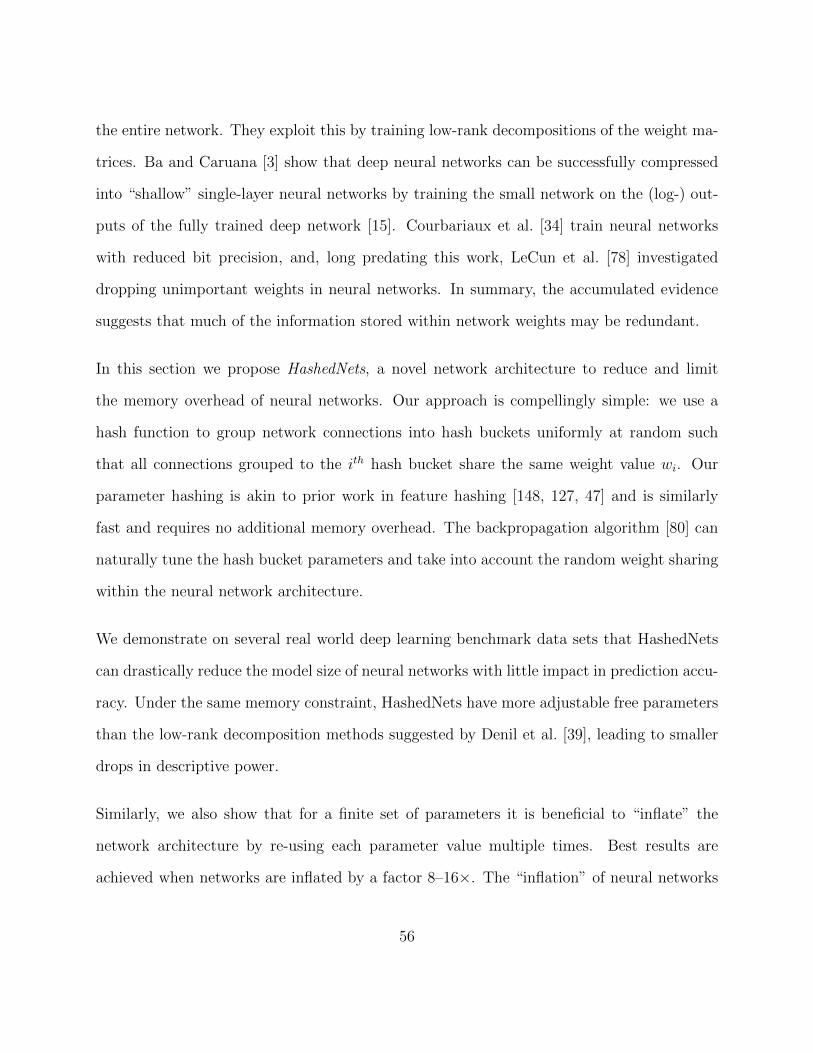
the entire network. They exploit this by training low-rank decompositions of the weight ma-

trices. Ba and Caruana [3] show that deep neural networks can be successfully compressed

into “shallow” single-layer neural networks by training the small network on the (log-) out-

puts of the fully trained deep network [15]. Courbariaux et al. [34] train neural networks

with reduced bit precision, and, long predating this work, LeCun et al. [78] investigated

dropping unimportant weights in neural networks. In summary, the accumulated evidence

suggests that much of the information stored within network weights may be redundant.

In this section we propose HashedNets, a novel network architecture to reduce and limit

the memory overhead of neural networks. Our approach is compellingly simple: we use a

hash function to group network connections into hash buckets uniformly at random such

that all connections grouped to the ith hash bucket share the same weight value wi. Our

parameter hashing is akin to prior work in feature hashing [148, 127, 47] and is similarly

fast and requires no additional memory overhead. The backpropagation algorithm [80] can

naturally tune the hash bucket parameters and take into account the random weight sharing

within the neural network architecture.

We demonstrate on several real world deep learning benchmark data sets that HashedNets

can drastically reduce the model size of neural networks with little impact in prediction accu-

racy. Under the same memory constraint, HashedNets have more adjustable free parameters

than the low-rank decomposition methods suggested by Denil et al. [39], leading to smaller

drops in descriptive power.

Similarly, we also show that for a finite set of parameters it is beneficial to “inflate” the

network architecture by re-using each parameter value multiple times. Best results are

achieved when networks are inflated by a factor 8–16×. The “inflation” of neural networks

56

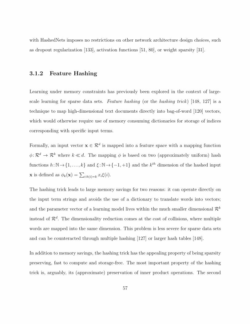
with HashedNets imposes no restrictions on other network architecture design choices, such

as dropout regularization [133], activation functions [51, 80], or weight sparsity [31].

3.1.2 Feature Hashing

Learning under memory constraints has previously been explored in the context of large-

scale learning for sparse data sets. Feature hashing (or the hashing trick) [148, 127] is a

technique to map high-dimensional text documents directly into bag-of-word [120] vectors,

which would otherwise require use of memory consuming dictionaries for storage of indices

corresponding with specific input terms.

Formally, an input vector x ∈ Rd is mapped into a feature space with a mapping function

φ :Rd → Rk where k� d. The mapping φ is based on two (approximately uniform) hash

functions h :N→{1, . . . , k} and ξ :N→{−1,+1} and the kth dimension of the hashed input

x is defined as φk(x) =∑

i:h(i)=k xiξ(i).

The hashing trick leads to large memory savings for two reasons: it can operate directly on

the input term strings and avoids the use of a dictionary to translate words into vectors;

and the parameter vector of a learning model lives within the much smaller dimensional Rk

instead of Rd. The dimensionality reduction comes at the cost of collisions, where multiple

words are mapped into the same dimension. This problem is less severe for sparse data sets

and can be counteracted through multiple hashing [127] or larger hash tables [148].

In addition to memory savings, the hashing trick has the appealing property of being sparsity

preserving, fast to compute and storage-free. The most important property of the hashing

trick is, arguably, its (approximate) preservation of inner product operations. The second

57

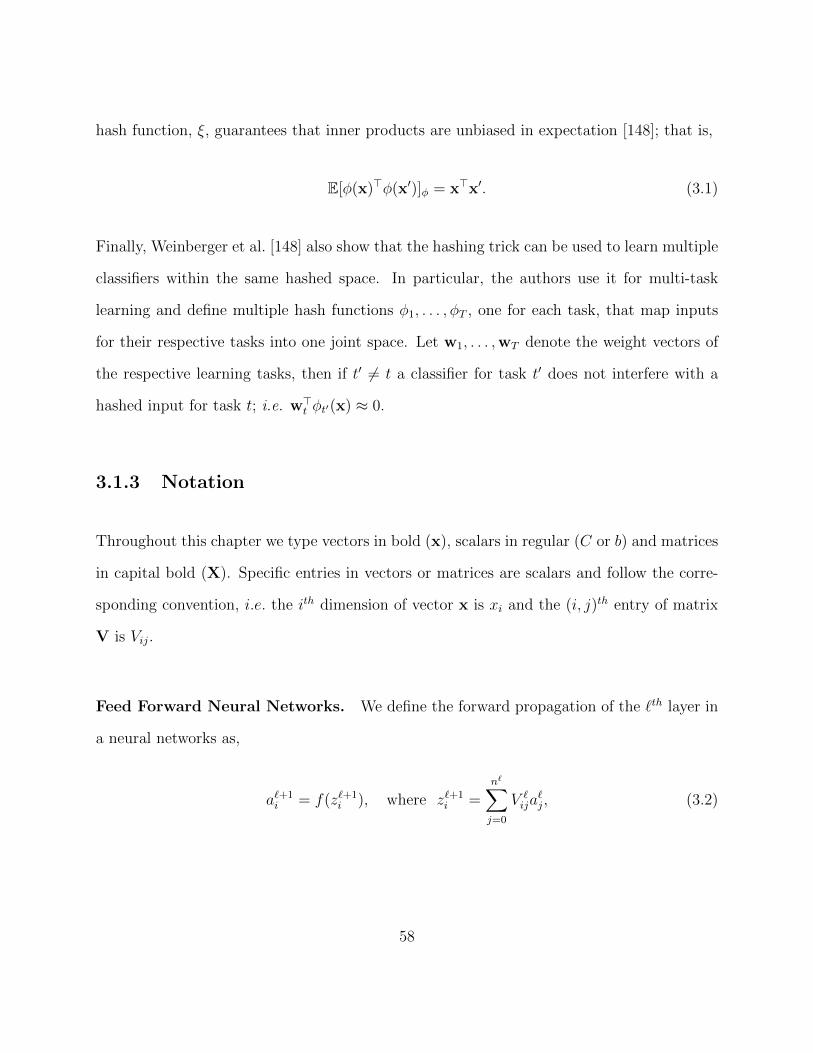
hash function, ξ, guarantees that inner products are unbiased in expectation [148]; that is,

E[φ(x)>φ(x′)]φ = x>x′. (3.1)

Finally, Weinberger et al. [148] also show that the hashing trick can be used to learn multiple

classifiers within the same hashed space. In particular, the authors use it for multi-task

learning and define multiple hash functions φ1, . . . , φT , one for each task, that map inputs

for their respective tasks into one joint space. Let w1, . . . ,wT denote the weight vectors of

the respective learning tasks, then if t′ 6= t a classifier for task t′ does not interfere with a

hashed input for task t; i.e. w>t φt′(x) ≈ 0.

3.1.3 Notation

Throughout this chapter we type vectors in bold (x), scalars in regular (C or b) and matrices

in capital bold (X). Specific entries in vectors or matrices are scalars and follow the corre-

sponding convention, i.e. the ith dimension of vector x is xi and the (i, j)th entry of matrix

V is Vij.

Feed Forward Neural Networks. We define the forward propagation of the `th layer in

a neural networks as,

a`+1i = f(z`+1

i ), where z`+1i =

n`∑j=0

V `ija

`j, (3.2)

58

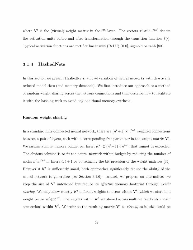
where V` is the (virtual) weight matrix in the `th layer. The vectors z`, a` ∈ Rn`denote

the activation units before and after transformation through the transition function f(·).

Typical activation functions are rectifier linear unit (ReLU) [100], sigmoid or tanh [80].

3.1.4 HashedNets

In this section we present HashedNets, a novel variation of neural networks with drastically

reduced model sizes (and memory demands). We first introduce our approach as a method

of random weight sharing across the network connections and then describe how to facilitate

it with the hashing trick to avoid any additional memory overhead.

Random weight sharing

In a standard fully-connected neural network, there are (n` + 1)×n`+1 weighted connections

between a pair of layers, each with a corresponding free parameter in the weight matrix V`.

We assume a finite memory budget per layer, K` � (n`+1)×n`+1, that cannot be exceeded.

The obvious solution is to fit the neural network within budget by reducing the number of

nodes n`, n`+1 in layers `, ` + 1 or by reducing the bit precision of the weight matrices [34].

However if K` is sufficiently small, both approaches significantly reduce the ability of the

neural network to generalize (see Section 3.1.6). Instead, we propose an alternative: we

keep the size of V` untouched but reduce its effective memory footprint through weight

sharing. We only allow exactly K` different weights to occur within V`, which we store in a

weight vector w`∈RK`. The weights within w` are shared across multiple randomly chosen

connections within V`. We refer to the resulting matrix V` as virtual, as its size could be

59

2.5 -0.7 -0.7 1.3

1.3 1.3 2.5 2.5

2.5 -0.7 1.3

real weights

virtual weight matrix

3.2 1.1 -0.5

real weights

1.1 3.2 3.2 -0.5

3.2 1.1 3.2 3.2

-0.5 1.1 3.2 1.1

3.2 -0.5 1.1 -0.5

virtual weight matrix

input

output

hiddenlayer

V1

V2

w1 w2

h1 h2

a11

a12

a13

a14 a2

4

a23

a22

a21

a31

a32

Figure 3.1: An illustration of a neural network with random weight sharing under compres-sion factor 1

4. The 16+9=25 virtual weights are compressed into 6 real weights. The colors

represent matrix elements that share the same weight value.

increased (i.e. nodes are added to hidden layer) without increasing the actual number of

parameters of the neural network.

Figure 3.1 shows a neural network with one hidden layer, four input units and two output

units. Connections are randomly grouped into three categories per layer and their weights

are shown in the virtual weight matrices V1 and V2. Connections belonging to the same

color share the same weight value, which are stored in w1 and w2, respectively. Overall,

the entire network is compressed by a factor 1/4, i.e. the 24 weights stored in the virtual

matrices V1 and V2 are reduced to only six real values in w1 and w2. On data with four

input dimensions and two output dimensions, a conventional neural network with six weights

would be restricted to a single (trivial) hidden unit.

60

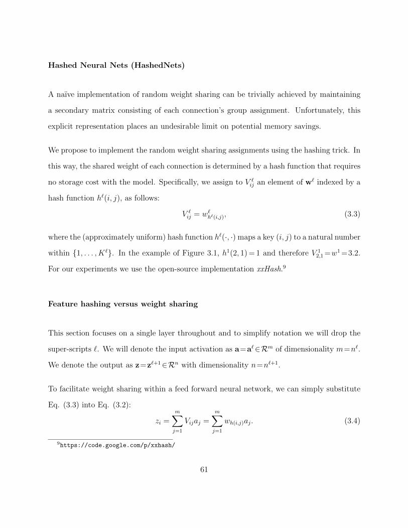
Hashed Neural Nets (HashedNets)

A naıve implementation of random weight sharing can be trivially achieved by maintaining

a secondary matrix consisting of each connection’s group assignment. Unfortunately, this

explicit representation places an undesirable limit on potential memory savings.

We propose to implement the random weight sharing assignments using the hashing trick. In

this way, the shared weight of each connection is determined by a hash function that requires

no storage cost with the model. Specifically, we assign to V `ij an element of w` indexed by a

hash function h`(i, j), as follows:

V `ij = w`h`(i,j), (3.3)

where the (approximately uniform) hash function h`(·, ·) maps a key (i, j) to a natural number

within {1, . . . , K`}. In the example of Figure 3.1, h1(2, 1) = 1 and therefore V 12,1 =w1 =3.2.

For our experiments we use the open-source implementation xxHash.9

Feature hashing versus weight sharing

This section focuses on a single layer throughout and to simplify notation we will drop the

super-scripts `. We will denote the input activation as a=a`∈Rm of dimensionality m=n`.

We denote the output as z=z`+1∈Rn with dimensionality n=n`+1.

To facilitate weight sharing within a feed forward neural network, we can simply substitute

Eq. (3.3) into Eq. (3.2):

zi =m∑j=1

Vijaj =m∑j=1

wh(i,j)aj. (3.4)

9https://code.google.com/p/xxhash/

61

Alternatively and more in line with previous work [148], we may interpret HashedNets in

terms of feature hashing. To compute zi, we first hash the activations from the previous

layer, a, with the hash mapping function φi(·) :Rm → RK . We then compute the inner

product between the hashed representation φi(a) and the parameter vector w,

zi = w>φi(a). (3.5)

Both w and φi(a) are K-dimensional, where K is the number of hash buckets in this layer.

The hash mapping function φi is defined as follows. The kth element of φi(a), i.e. [φi(a)]k,

is the sum of variables hashed into bucket k:

[φi(a)]k =∑

j:h(i,j)=k

aj. (3.6)

Starting from Eq. (3.5), we show that the two interpretations (Eq. (3.4) and (3.5)) are

equivalent:

zi =K∑k=1

wk [φi(a)]k =K∑k=1

wk∑

j:h(i,j)=k

aj

=m∑j=1

K∑k=1

wkajδ[h(i,j)=k]

=m∑j=1

wh(i,j)aj.

The final term is equivalent to Eq. (3.4).

Sign factor. With this equivalence between random weight sharing and feature hashing

on input activations, HashedNets inherit several beneficial properties of the feature hashing.

62

Weinberger et al. [148] introduce an additional sign factor ξ(i, j) to remove the bias of hashed

inner-products due to collisions. For the same reasons we multiply (3.3) by the sign factor

ξ(i, j) for parameterizing V [148]:

Vij = wh(i,j)ξ(i, j), (3.7)

where ξ(i, j) :N → ±1 is a second hash function independent of h. Incorporating ξ(i, j) to

feature hashing and weight sharing does not change the equivalence between them as the

proof in the previous section still holds with the sign term (details omitted for improved

readability).

Sparsity. As pointed out in Shi et al. [127] and Weinberger et al. [148], feature hashing

is most effective on sparse feature vectors since the number of hash collisions is minimized.

We can encourage this effect in the hidden layers with sparsity inducing transition functions,

e.g. rectified linear units (ReLU) [51] or through specialized regularization [17, 10]. In our

implementation, we use ReLU transition functions throughout, as they have also been shown

to often result in superior generalization performance in addition to their sparsity inducing

properties [51].

Alternative neural network architectures. While this work focuses on general, fully

connected feed forward neural networks, the technique of HashedNets could naturally be ex-

tended to other kinds of neural networks, such as recurrent neural networks [107] or others [6].

It can also be used in conjunction with other approaches for neural network compression. All

63

weights can be stored with low bit precision [34, 56], edges could be removed [30] and Hashed-

Nets can be trained on the outputs of larger networks [3] — yielding further reductions in

memory requirements.

Training HashedNets

Training HashedNets is equivalent to training a standard neural network with equality con-

straints for weight sharing. Here, we show how to (a) compute the output of a hash layer

during the feed-forward phase, (b) propagate gradients from the output layer back to input

layer, and (c) compute the gradient over the shared weights w` during the back propagation

phase. We use dedicated hash functions between layers ` and ` + 1, and denote them as h`

and ξ`.

Output. Adding the hash functions h`(·, ·) and ξ`(·) and the weight vectors w` into the

feed forward update (3.2) results in the following forward propagation rule:

a`+1i = f

n`∑j

w`h`(i,j)ξ`(i, j)a`j

. (3.8)

Error term. Let L denote the loss function for training the neural network, e.g. cross

entropy or the quadratic loss [6]. Further, let δ`j denote the gradient of L over activation

j in layer `, also known as the error term. Without shared weights, the error term can be

expressed as δ`j =(∑n`+1

i=1 V `ijδ

`+1i

)f ′(z`j), where f ′(·) represents the first derivative of the

64

transition function f(·). If we substitute Eq. (3.7) into the error term we obtain:

δ`j =

n`+1∑i=1

ξ`(i, j)w`h`(i,j)δ`+1i

f ′(z`j). (3.9)

Gradient over parameters. To compute the gradient of L with respect to a weight w`k

we need the two gradients,

∂L∂V `

ij

= a`jδ`+1i and

∂V `ij

∂w`k= ξ`(i, j)δh`(i,j)=k. (3.10)

Here, the first gradient is the standard gradient of a (virtual) weight with respect to an

activation unit and the second gradient ties the virtual weight matrix to the actual weights

through the hashed map. Combining these two, we obtain

∂L∂w`k

=∑i,j

∂L∂V `

ij

∂V `ij

∂w`k(3.11)

=n`+1∑i=1

∑j

a`jδ`+1i ξ`(i, j)δh`(i,j)=k. (3.12)

3.1.5 Related Work

Deep neural networks have achieved great progress on a wide variety of real-world appli-

cations, including image classification [72, 41, 124, 158], object detection [50, 141], image

retrieval [111], speech recognition [63, 54, 97], and text representation [96].

There have been several previous attempts to reduce the complexity of neural networks under

a variety of contexts. Arguably the most popular method is the widely used convolutional

65

neural network [130]. In the convolutional layers, the same filter is applied to every receptive

field, both reducing model size and improving generalization performance. The incorporation

of pooling layers [157] can reduce the number of connections between layers in domains

exhibiting locality among input features, such as images. Autoencoders [52] share the notion

of tied weights by using the same weights for the encoder and decoder (up to transpose).

Other methods have been proposed explicitly to reduce the number of free parameters in

neural networks, but not necessarily for reducing memory overhead. Nowlan and Hinton

[103] introduce soft weight sharing for regularization in which the distribution of weight

values is modeled as a Gaussian mixture. The weights are clustered such that weights in the

same group have similar values. Since weight values are unknown before training, weights

are clustered during training. This approach is fundamentally different from HashedNets

since it requires auxiliary parameters to record the group membership for every weight.

Instead of sharing weights, LeCun et al. [78] introduce “optimal brain damage” to directly

drop unimportant weights. This approach requires auxiliary parameters for storing the

sparse weights and needs retraining time to fine-tune the resulting architecture. Ciresan

et al. [30] demonstrate in their experiments that randomly removing connections leads to

superior empirical performance, which shares the same spirit of HashedNets.

Courbariaux et al. [34] and Gupta et al. [56] learn networks with reduced numerical precision

for storing model parameters (e.g. 16-bit fixed-point representation [56] for a compression

factor of 14

over double-precision floating point). Experiments indicate little reduction in

accuracy compared with models trained with double-precision floating point representation.

These methods can be readily incorporated with HashedNets, potentially yielding further

reduction in model storage size.

66

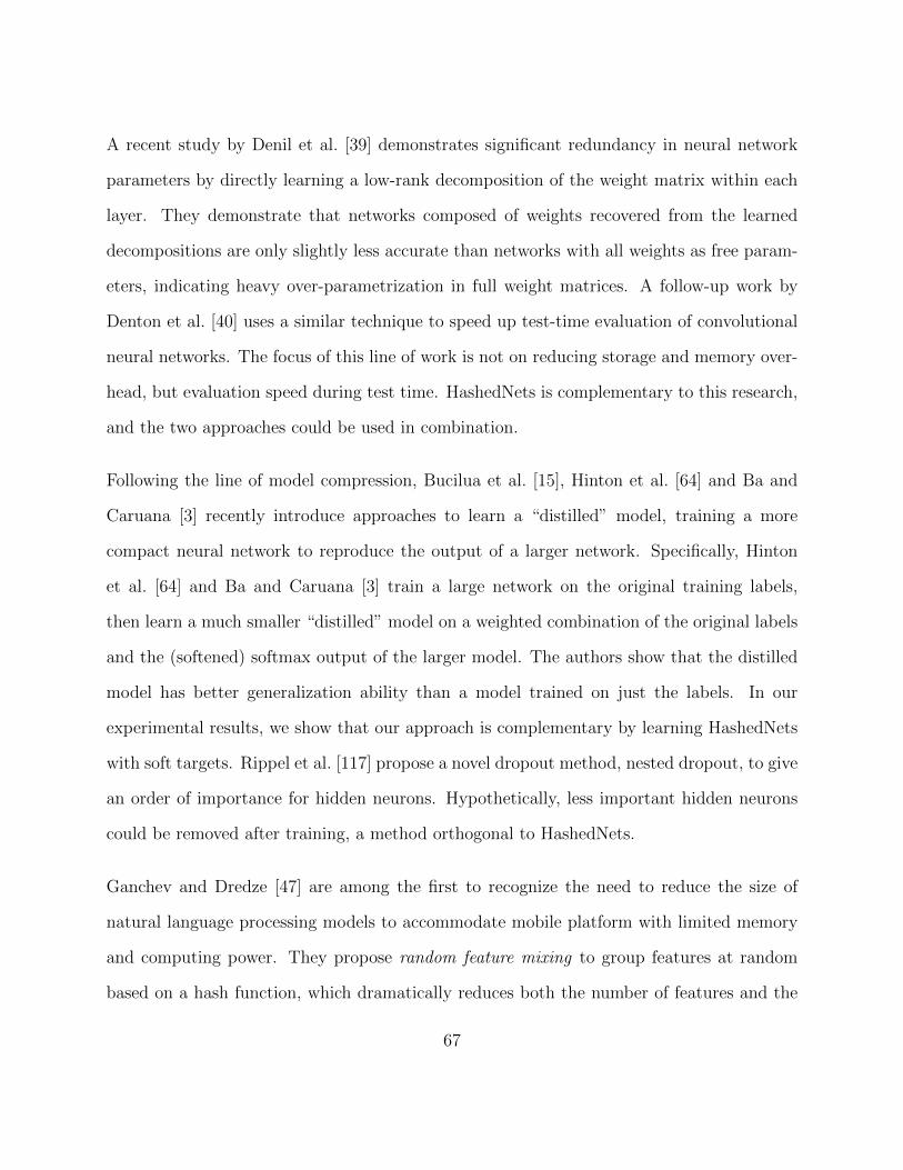
A recent study by Denil et al. [39] demonstrates significant redundancy in neural network

parameters by directly learning a low-rank decomposition of the weight matrix within each

layer. They demonstrate that networks composed of weights recovered from the learned

decompositions are only slightly less accurate than networks with all weights as free param-

eters, indicating heavy over-parametrization in full weight matrices. A follow-up work by

Denton et al. [40] uses a similar technique to speed up test-time evaluation of convolutional

neural networks. The focus of this line of work is not on reducing storage and memory over-

head, but evaluation speed during test time. HashedNets is complementary to this research,

and the two approaches could be used in combination.

Following the line of model compression, Bucilua et al. [15], Hinton et al. [64] and Ba and

Caruana [3] recently introduce approaches to learn a “distilled” model, training a more

compact neural network to reproduce the output of a larger network. Specifically, Hinton

et al. [64] and Ba and Caruana [3] train a large network on the original training labels,

then learn a much smaller “distilled” model on a weighted combination of the original labels

and the (softened) softmax output of the larger model. The authors show that the distilled

model has better generalization ability than a model trained on just the labels. In our

experimental results, we show that our approach is complementary by learning HashedNets

with soft targets. Rippel et al. [117] propose a novel dropout method, nested dropout, to give

an order of importance for hidden neurons. Hypothetically, less important hidden neurons

could be removed after training, a method orthogonal to HashedNets.

Ganchev and Dredze [47] are among the first to recognize the need to reduce the size of

natural language processing models to accommodate mobile platform with limited memory

and computing power. They propose random feature mixing to group features at random

based on a hash function, which dramatically reduces both the number of features and the

67

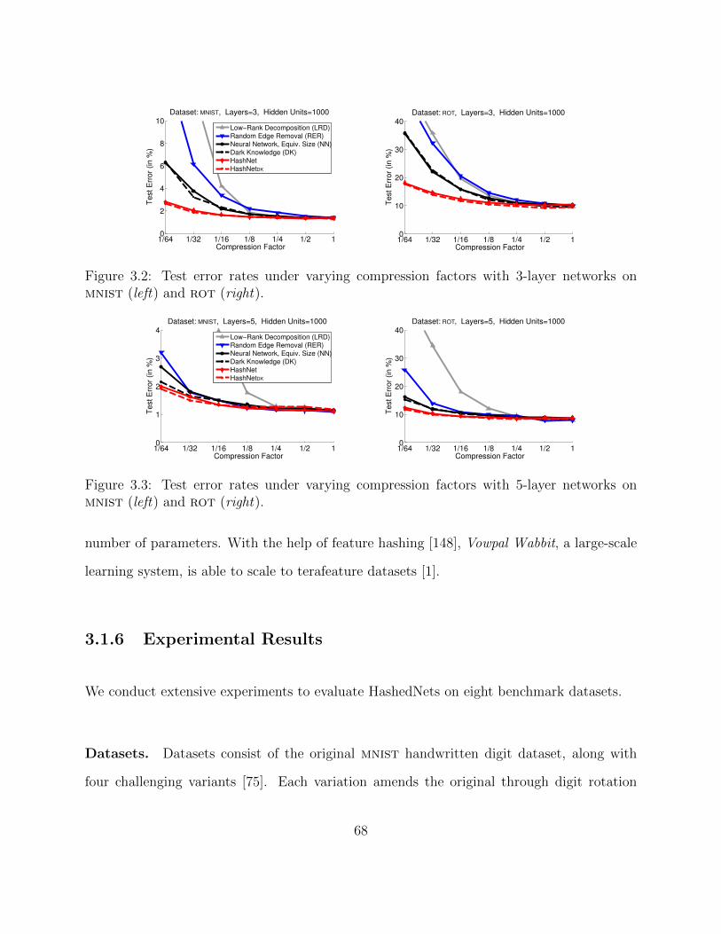
1/64 1/32 1/16 1/8 1/4 1/2 10

2

4

6

8

10Dataset: MNIST, Layers=3, Hidden Units=1000

Compression Factor

Test E

rror

(in %

)

Low−Rank Decomposition (LRD)Random Edge Removal (RER)Neural Network, Equiv. Size (NN)

Dark Knowledge (DK)HashNetHashNetDK

1/64 1/32 1/16 1/8 1/4 1/2 10

10

20

30

40Dataset: ROT, Layers=3, Hidden Units=1000

Compression Factor

Test E

rror

(in %

)

Figure 3.2: Test error rates under varying compression factors with 3-layer networks onmnist (left) and rot (right).

1/64 1/32 1/16 1/8 1/4 1/2 10

1

2

3

4Dataset: MNIST, Layers=5, Hidden Units=1000

Compression Factor

Test E

rror

(in %

)

Low−Rank Decomposition (LRD)Random Edge Removal (RER)Neural Network, Equiv. Size (NN)

Dark Knowledge (DK)HashNetHashNetDK

1/64 1/32 1/16 1/8 1/4 1/2 10

10

20

30

40Dataset: ROT, Layers=5, Hidden Units=1000

Compression Factor

Test E

rror

(in %

)

Figure 3.3: Test error rates under varying compression factors with 5-layer networks onmnist (left) and rot (right).

number of parameters. With the help of feature hashing [148], Vowpal Wabbit, a large-scale

learning system, is able to scale to terafeature datasets [1].

3.1.6 Experimental Results

We conduct extensive experiments to evaluate HashedNets on eight benchmark datasets.

Datasets. Datasets consist of the original mnist handwritten digit dataset, along with

four challenging variants [75]. Each variation amends the original through digit rotation

68

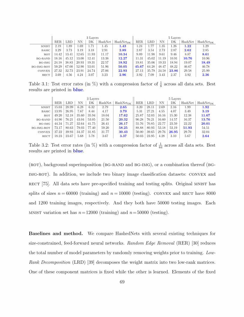
3 Layers 5 LayersRER LRD NN DK HashNet HashNetDK RER LRD NN DK HashNet HashNetDK

mnist 2.19 1.89 1.69 1.71 1.45 1.43 1.24 1.77 1.35 1.26 1.22 1.29basic 3.29 3.73 3.19 3.18 2.91 2.89 2.87 3.54 2.73 2.87 2.62 2.85rot 14.42 13.41 12.65 11.93 11.17 10.34 9.89 11.98 9.61 9.46 8.87 8.61

bg-rand 18.16 45.12 13.00 12.41 13.38 12.27 11.31 45.02 11.19 10.91 10.76 10.96bg-img 24.18 38.83 20.93 19.31 22.57 18.92 19.81 35.06 19.33 18.94 19.07 18.49

bg-img-rot 59.29 67.00 52.90 53.01 51.96 50.05 45.67 64.28 48.47 48.22 46.67 46.78convex 27.32 32.73 23.91 24.74 27.06 22.93 27.13 35.79 24.58 23.86 29.58 25.99

rect 3.69 4.56 4.24 3.07 3.23 2.96 3.92 7.09 3.43 2.37 3.92 2.36

Table 3.1: Test error rates (in %) with a compression factor of 18

across all data sets. Bestresults are printed in blue.

3 Layers 5 LayersRER LRD NN DK HashNet HashNetDK RER LRD NN DK HashNet HashNetDK

mnist 15.03 28.99 6.28 6.32 2.79 2.65 3.20 28.11 2.69 2.16 1.99 1.92basic 13.95 26.95 7.67 8.44 4.17 3.79 5.31 27.21 4.55 4.07 3.49 3.19rot 49.20 52.18 35.60 35.94 18.04 17.62 25.87 52.03 16.16 15.30 12.38 11.67

bg-rand 44.90 76.21 43.04 53.05 21.50 20.32 90.28 76.21 16.60 14.57 16.37 13.76bg-img 44.34 71.27 32.64 41.75 26.41 26.17 55.76 70.85 22.77 23.59 22.22 20.01

bg-img-rot 73.17 80.63 79.03 77.40 59.20 58.25 88.88 80.93 53.18 53.19 51.93 54.51convex 37.22 39.93 34.37 31.85 31.77 30.43 50.00 39.65 29.76 26.95 29.70 32.04

rect 18.23 23.67 5.68 5.78 3.67 3.37 50.03 23.95 4.28 3.10 5.67 2.64

Table 3.2: Test error rates (in %) with a compression factor of 164

across all data sets. Bestresults are printed in blue.

(rot), background superimposition (bg-rand and bg-img), or a combination thereof (bg-

img-rot). In addition, we include two binary image classification datasets: convex and

rect [75]. All data sets have pre-specified training and testing splits. Original mnist has

splits of sizes n= 60000 (training) and n= 10000 (testing). convex and rect have 8000

and 1200 training images, respectively. And they both have 50000 testing images. Each

mnist variation set has n=12000 (training) and n=50000 (testing).

Baselines and method. We compare HashedNets with several existing techniques for

size-constrained, feed-forward neural networks. Random Edge Removal (RER) [30] reduces

the total number of model parameters by randomly removing weights prior to training. Low-

Rank Decomposition (LRD) [39] decomposes the weight matrix into two low-rank matrices.

One of these component matrices is fixed while the other is learned. Elements of the fixed

69

1 2 4 8 16 32 641

2

3

4

Test E

rror

(in %

)

Expansion Factor

Dataset: MNIST, Layers=3, Hidden Units=50

Neural Network, Equiv. Size (NN)

Low−Rank Decomposition (LRD)

Random Edge Removal (RER)

HashNet

1 2 4 8 16 32 641

2

3

4

Test E

rror

(in %

)

Expansion Factor

Dataset: MNIST, Layers=5, Hidden Units=50

Figure 3.4: Test error rates with fixed storage but varying expansion factors on mnist with3 layers (left) and 5 layers (right).

matrix are generated according to a zero-mean Gaussian distribution with standard deviation

1√n`

with n` inputs to the layer.

Each model is compared against a standard neural network with an equivalent number of

stored parameters, Neural Network (Equivalent-Size) (NN). For example, for a network with

a single hidden layer of 1000 units and a storage compression factor of 110

, we adopt a size-

equivalent baseline with a single hidden layer of 100 units. For deeper networks, all hidden

layers are shrunk at the same rate until the number of stored parameters equals the target

size. In a similar manner, we examine Dark Knowledge (DK) [64, 3] by training a distilled

model to optimize the cross entropy with both the original labels and soft targets gener-

ated by the corresponding full neural network (compression factor 1). The distilled model

structure is chosen to be same as the “equivalent-sized” network (NN) at the corresponding

compression rate.

Finally, we examine our method under two settings: learning hashed weights with the original

training labels (HashNet) and with combined labels and DK soft targets (HashNetDK). In

all cases, memory and storage consumption is defined strictly in terms of free parameters.

70

As such, we count the fixed low rank matrix in the Low-Rank Decomposition method as

taking no memory or storage (providing this baseline a slight advantage).

Experimental setting. HashedNets and all accompanying baselines were implemented

using Torch7 [33] and run on NVIDIA GTX TITAN graphics cards with 2688 cores and 6GB

of global memory. We use 32 bit precision throughout but note that the compression rates of

all methods may be improved with lower precision [34, 56]. We verify all implementations by

numerical gradient checking. Models are trained via stochastic gradient descent (mini-batch

size of 50) with dropout and momentum. ReLU is adopted as the activation function for all

models. Hyperparameters are selected for all algorithms with Bayesian optimization [132]

and hand tuning on 20% validation splits of the training sets. We use the open source

Bayesian Optimization MATLAB implementation “bayesopt.m” from Gardner et al. [48].10

Results with varying compression. Figures 3.2 and 3.3 show the performance of all

methods on mnist and the rot variant with different compression factors on 3-layer (1

hidden layer) and 5-layer (3 hidden layers) neural networks, respectively. Each hidden layer

contains 1000 hidden units. The x-axis in each figure denotes the fractional compression fac-

tor. For HashedNets and the low rank decomposition and random edge removal compression

baselines, this means we fix the number of hidden units (n`) and vary the storage budget

(K`) for the weights (w`).

We make several observations: The accuracy of HashNet and HashNetDK outperforms all

other baseline methods, especially in the most interesting case when the compression factor is

10http://tinyurl.com/bayesopt

71

small (i.e. very small models). Both compression baseline algorithms, low rank decomposi-

tion and random edge removal, tend to not outperform a standard neural network with fewer

hidden nodes (black line), trained with dropout. For smaller compression factors, random

edge removal likely suffers due to a significant number of nodes being entirely disconnected

from neighboring layers. The size-matched NN is consistently the best performing baseline,

however its test error is significantly higher than that of HashNet especially at small com-

pression rates. The use of Dark Knowledge training improves the performance of HashedNets

and the standard neural network. Of all methods, only HashNet and HashNetDK maintain

performance for small compression factors.

For completeness, we show the performance of all methods on all eight datasets in Table 3.1

for compression factor 18

and Table 3.2 for compression factor 164

. HashNet and HashNetDK

outperform other baselines in most cases, especially when the compression factor is very

small (Table 3.2). With a compression factor of 164

on average only 0.5 bits of information

are stored per (virtual) parameter. Also note that non-neural network classifiers [153, 24]

with the same model size cannot compete with this result either.

Results with fixed storage. We also experiment with the setting where the model size

is fixed and the virtual network architecture is “inflated”. Essentially we are fixing K` (the

number of “real” weights in w`), and vary the number of hidden nodes (n`). An expansion

factor of 1 denotes the case where every virtual weight has a corresponding “real” weight,

(n` + 1)n`+1 =K`. Figure 3.4 shows the test error rate under various expansion rates of a

network with one hidden layer (left) and three hidden layers (right). In both scenarios we

fix the number of real weights to the size of a standard fully-connected neural network with

50 hidden units in each hidden layer whose test error is shown by the black dashed line.

72

With no expansion (at expansion rate 1), different compression methods perform differently.

At this point edge removal is identical to a standard neural network and matches its results.

If no expansion is performed, the HashNet performance suffers from collisions at no benefit.

Similarly the low-rank method still randomly projects each layer to a random feature space

with same dimensionality.

For expansion rates greater 1, all methods improve over the fixed-sized neural network. There

is a general trend that more expansion decreases the test error until a “sweet-spot” after

which additional expansion tends to hurt. The test error of the HashNet neural network

decreases substantially through the introduction of more “virtual” hidden nodes, despite

that no additional parameters are added. In the case of the 5-layer neural network (right)

this trend is maintained to an expansion factor of 16×. One could hypothetically increase

n` arbitrarily for HashNet, however, in the limit, too many hash collisions would result in

increasingly similar gradient updates for all weights in w.

The benefit from expanding a network cannot continue forever. In the random edge removal

the network will become very sparsely connected; the low-rank decomposition approach will

eventually lead to a decomposition into rank-1 matrices. HashNet also respects this trend,

but is much less sensitive when the expansion goes up. Best results are achieved when

networks are inflated by a factor 8−16×.

3.1.7 Conclusion

Prior work shows that weights learned in neural networks can be highly redundant [39].

In this chapter, we have presented HashedNets to exploit this property to create neural

networks with “virtual” connections that seemingly exceed the storage limits of the trained

73

model. This can have surprising effects. Figure 3.4 in Section 3.1.6 shows the test error of

neural networks can drop nearly 50%, from 3% to 1.61%, through expanding the number of

weights “virtually” by a factor 8×. Although the collisions (or weight-sharing) might serve

as a form of regularization, we can probably safely ignore this effect as both networks (with

and without expansion) were also regularized with dropout [133] and the hyper-parameters

were carefully fine-tuned through Bayesian optimization.

So why should additional virtual layers help? One answer is that they probably truly increase

the expressiveness of the neural network. As an example, imagine we are provided with a

neural network with 100 hidden nodes. The internal weight matrix has 10000 weights. If we

add another set of m hidden nodes, this increases the expressiveness of the network. If we

require all weights of connections to these m additional nodes to be “re-used” from the set of

existing weights, it is not a strong restriction given the large number of weights in existence.

In addition, the backprop algorithm can adjust the shared weights carefully to have useful

values for all their occurrences.

3.2 Compressing convolutional neural network in the

frequency domain

3.2.1 Introduction

We have introduced using HashedNets to compress neural networks. In this section, we

aim to compress convolutional neural networks (CNN). Although CNNs have been known

for a quarter of a century [46], only recently have their superb generalization abilities been

74

accepted widely across the machine learning and computer vision communities. This broad

acceptance coincides with the release of very large collections of labeled data [38]. Deep

networks and CNNs are particularly well suited to learn from large quantities of data, in

part because they can have arbitrarily many parameters. As data sets grow, so do model

sizes. In 2012, the first winner of the ImageNet competition that used a CNN had already

240MB of parameters and the most recent winning model, in 2014, required 567MB [131].

Independently, same as described in Section 3.1, there has been another parallel shift of

computing from servers and workstations to mobile platforms. As of January 2014 there

have already been more web searches through smart phones than computers11. Today speech

recognition is primarily used on cell phones with intelligent assistants such as Apple’s Siri,

Google Now or Microsoft’s Cortana. As this trend continues, we are expecting applications

of CNNs to also shift increasingly towards mobile devices which have tight memory and

storage limitations.

Of course, HashedNets presented in Section 3.1 also applies to convolutional layers by random

weight sharing with the hashing trick. However, it does not harness the distinct property of

CNNs, which is the local smoothness of the parameters in the filters. Building on Hashed-

Nets, in this section we propose a novel approach for neural network compression targeted

especially for CNNs. Due to the nature of local pixel correlation in images (i.e. spatial lo-

cality), filters in CNNs tend to be smooth. We transform these filters into frequency domain

with the discrete cosine transform (DCT) [109]. In frequency space, the filters are naturally

dominated by low frequency components. Our compression takes this smoothness property

into account and randomly hashes the frequency components of all CNN filters at a given

layer into one common set of hash buckets. All components inside one hash bucket share the

11http://tinyurl.com/omd58sq

75

same value. As lower frequency components are more pronounced than higher frequencies,

we allow collisions only between similar frequencies and allocate fewer hash buckets for the

high frequencies (which are less important).

Our approach has several compelling properties: 1. The number of parameters in the CNN

is independent of the number of convolutional filters; 2. During testing we only need to add

a low-cost hash function and the inverse DCT transformation to any existing CNN code

for filter reconstruction; 3. During training, the hashed weights can be learned with simple

back-propagation [6]—the gradient of a hash bucket value is the sum of gradients of all

hashed frequency components in that bucket.

We evaluate our compression scheme on eight deep learning image benchmark data sets

and compare against four competitive baselines. Although all compression schemes lead to

lower test accuracy as the compression increases, our FreshNets method is by far the most

effective compression method and yields the lowest generalization error rates on almost all

classification tasks.

3.2.2 Background

Discrete Cosine Transform (DCT) [109]. Methods built on the DCT are widely

used for compressing images and movies, including forming the standard technique for

JPEG [142]. DCT expresses a function as a weighted combination of sinusoids of different

phases/frequencies where the weight of each sinusoid reflects the magnitude of the corre-

sponding frequency in the input. When employed with sufficient numerical precision and

without quantization or other compression operations, the DCT and inverse DCT (project-

ing frequency inputs back to the spatial domain) are lossless. Compression is made possible

76

in images by local smoothness of pixels (e.g. a blue sky) which can be well represented

regionally by fewer non-zero frequency components. Though highly related to the discrete

Fourier transformation (DFT), DCT is often preferable for compression tasks because of its

spectral compaction property where weights for most images tend to be concentrated in a

few low-frequency components of the DCT [109]. Further, the DCT transformation yields a

real-valued representation, unlike the DFT whose representation has imaginary components.

Given an input matrix V ∈Rd×d, the corresponding matrix V ∈Rd×d in frequency domain

after DCT is defined as:

Vj1j2 = sj1sj2

d−1∑i1=0

d−1∑i2=0

c(i1, i2, j1, j2) Vi1i2 , (3.13)

where c(i1, i2, j1, j2) = cos

[π

d

(i1 +

1

2

)j1

]cos

[π

d

(i2 +

1

2

)j2

]is the cosine basis function, and sj =

√1d

when j = 0 and sj =√

2d

otherwise. We use the

shorthand fdct to denote the DCT operation in Eq. (3.13), i.e. V = fdct(V ). The inverse

DCT converts V from the frequency domain back to the spatial domain, reconstructing V

without loss:

Vi1i2 =d−1∑j1=0

d−1∑j2=0

sj1sj2 c(i1, i2, j1, j2) Vj1j2 . (3.14)

We denote the inverse DCT function in Eq. (3.14) as f−1dct, i.e. V = f−1dct(V).

3.2.3 Frequency-Sensitive Hashed Nets

Here we present FreshNets, a method for using weight sharing to reduce the model size (and

memory demands) of convolutional neural networks. Similar to HashedNets, we achieve

smaller models by randomly forcing weights throughout the network to share identical values.

77

wei

ghts

2.9 1.11.53.2 -0.52.5 -2.1 1.3

3.2

1.1

1.1

-0.5

2.5

-2.1

1.5

-0.5

1.3

2.9

1.1

1.1

-0.5

-2.1

2.5

-0.5

1.5

1.3

2.6

0.4

2.3

-1.6

-0.7

1.1

2.4

2.2

0.9

2.0

1.2

0.7

3.5

1.5

-1.8

1.4

2.2

0.4

f�1dct

freq

uenc

y do

mai

nsp

atia

l dom

ain

V

V

w

reconstruct virtual frequencies

map to spatial domainf�1

dct

Filter 1 Filter 2

w0 w1 w2 w3 w4

hj , ⇠hj , ⇠

Figure 3.5: A schematic illustration of FreshNets. Two spatial filters are re-constructedfrom the frequency weights in vector w. The frequency weights are accessed with two hashfunctions and then transformed to the spatial domain. The vector w is partitioned intosub-vectors wj shared by all entries with similar frequency (corresponding to index sumj = j1 + j2). Colors indicate which hash bucket was accessed.

Unlike previous work, we implement the weight sharing and gradient updates of convolutional

filters in the frequency domain. These sharing constraints are made prior to training, and

we learn frequency weights under the sharing assignments. Since the assignments are made

with a hash function, they incur no additional storage.

Filters in spatial and frequency domain. Let the matrix V k`∈Rd×d denote the weight

matrix of the d×d convolutional filter that connects the kth input plane to the `th output

plane. (For notational convenience we assume square filters and only consider the filters in a

single layer of the network.) The weights of all filters in a convolutional layer can be denoted

by a 4-dimensional tensor V ∈Rm×n×d×d where m and n are the number of input planes and

output planes, respectively, resulting in a total of m × n × d2 parameters. Convolutional

filters can be represented equivalently in either the spatial or frequency domain, mapping

between the two via the DCT and its inverse. We denote the filter in frequency domain

78

as Vk` = fdct(Vk`) ∈ Rd×d and recover the original spatial representation through V k` =

f−1dct(Vk`), as defined in Eq. (3.13) and (3.14), respectively. The tensor of all filters is

denoted V∈Rm×n×d×d.

Random Weight Sharing by Hashing. We would like to reduce the number of model

parameters to exactly K values stored in a weight vector w∈RK , where K � m× n× d2.

To achieve this, we randomly assign a value from w to each filter frequency weight in V .

A naıve implementation of this random weight sharing would introduce an auxiliary matrix

for V to track the weight assignments, using to significant additional memory. To address

this problem, FreshNets adopts the hashing trick used in HashedNets (See Section 3.1) to

(pseudo-)randomly assign shared parameters. Using the hashing trick, we tie each filter

weight Vk`j1j2 to an element of w indexed by the output of a hash function h(·):

Vk`j1,j2 = ξ(k, `, j1, j2) wh(k,`,j1,j2), (3.15)

where h(k, `, j1, j2) ∈ {1, · · · , K}, and ξ(k, `, j1, j2) ∈ {±1} is a sign factor computed by

a second hash function ξ(·) to preserve inner-products in expectation as described in Sec-

tion 3.1.2. With the mapping in Eq. (3.15), we can implement shared parameter assignments

with no additional storage cost. (For a schematic illustration, see Figure 3.5. The figure also

incorporates a frequency sensitive hashing scheme discussed later in this section.)

Gradients over Shared Frequency Weights. Typical convolutional neural networks

learn filters in the spatial domain. As our shared weights are stored in the frequency domain,

we derive the gradient with respect to filter parameters in frequency space. Following Eq.

(3.14), we express the gradient of parameters in the spatial domain w.r.t. their counterparts

79

in the frequency domain:

∂V k`i1i2

∂Vk`j1j2= sj1sj2 c(i1, i2, j1, j2). (3.16)

Let L be the loss function adopted for training. Using standard back-propagation, we can

derive the gradient w.r.t. filter parameters in the spatial domain, ∂L∂V k`

i1i2

. By the chain rule

with Eq. (3.16), we express the gradient of L in the frequency domain:

∂L∂Vk`j1j2

=d−1∑i1=0

d−1∑i2=0

∂L∂V k`

i1i2

∂V k`i1i2

∂Vk`j1j2= sj1sj2

d−1∑i1=0

d−1∑i2=0

c(i1, i2, j1, j2)∂L∂V k`

i1i2

. (3.17)

Comparing with Eq. (3.13), we see that the gradient in the frequency domain is merely the

DCT of the gradient in the spatial domain:

∂L∂Vk`

= fdct

(∂L∂V k`

). (3.18)

We compute gradient for each shared weight wh by simply summing over the gradient at

each filter parameter where the weight is assigned, i.e. all Vk`j1j2 where h = h(k, `, j1, j2):

∂L∂wh

=m∑k=0

n∑`=0

d−1∑j1=0

d−1∑j2=0

∂L∂Vk`j1j2

∂Vk`j1j2∂wh

=∑

k,`,j1,j2:h=h(k,`,j1,j2)

ξ(k, `, j1, j2)

[fdct

(∂L∂V k`

)]j1j2

(3.19)

where [A]j1j2 denotes the (j1, j2) entry in matrix A.

Frequency Sensitive Hashing. Figure 3.6 shows a filter in spatial (left) and frequency

(right) domains. In the spatial domain CNN filters are smooth [72] due to the local pixel

smoothness in natural images. In the frequency domain this corresponds to components with

large magnitudes in the low frequencies, depicted in the upper left half of Vk` in Figure 3.6.

80

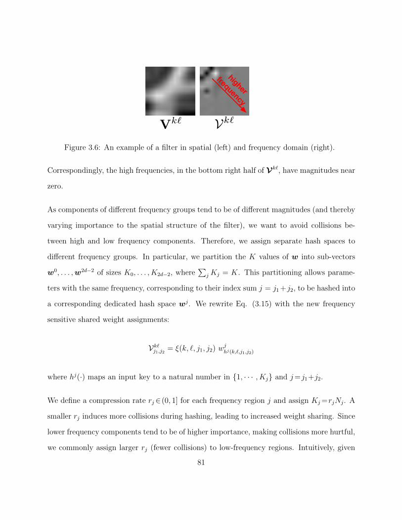
higherfrequency

Vk` Vk`

Figure 3.6: An example of a filter in spatial (left) and frequency domain (right).

Correspondingly, the high frequencies, in the bottom right half of Vk`, have magnitudes near

zero.

As components of different frequency groups tend to be of different magnitudes (and thereby

varying importance to the spatial structure of the filter), we want to avoid collisions be-

tween high and low frequency components. Therefore, we assign separate hash spaces to

different frequency groups. In particular, we partition the K values of w into sub-vectors

w0, . . . ,w2d−2 of sizes K0, . . . , K2d−2, where∑

jKj = K. This partitioning allows parame-

ters with the same frequency, corresponding to their index sum j = j1 +j2, to be hashed into

a corresponding dedicated hash space wj. We rewrite Eq. (3.15) with the new frequency

sensitive shared weight assignments:

Vk`j1,j2 = ξ(k, `, j1, j2) wjhj(k,`,j1,j2)

where hj(·) maps an input key to a natural number in {1, · · · , Kj} and j=j1+j2.

We define a compression rate rj∈(0, 1] for each frequency region j and assign Kj =rjNj. A

smaller rj induces more collisions during hashing, leading to increased weight sharing. Since

lower frequency components tend to be of higher importance, making collisions more hurtful,

we commonly assign larger rj (fewer collisions) to low-frequency regions. Intuitively, given

81

a size budget for the whole convolutional layer, we want to squeeze the hash space of high

frequency region to save space for low frequency regions. These compression rates can either

be assigned by hand or determined programmatically by cross-validation, as demonstrated

in Section 3.2.5.

3.2.4 Related Work

Several recent studies have confirmed that there is significant redundancy in the parameters

learned in deep neural networks. Recent work by Denil et al. [39] learns parameters in fully-

connected layers after decomposition into two low-rank matrices, i.e. W =AB where W ∈

Rm×n, A∈Rm×k and B ∈ Rk×n. In this way, the original O(mn) parameters could be stored

with O(k(m + n)) storage, where k � min(m,n). Several works apply related approaches

to speed up the evaluation time with convolutional neural networks. Two works propose to

approximate convolutional filters by a weighted linear combination of basis filters [116, 66].

In this setting, the convolution operation only needs to be performed with the small set of

basis filters. The desired output feature maps are computed by matrix multiplication as

the weighted sum of these basis convolutions. Further speedup can be achieved by learning

rank-one basis filters so that the convolution operations are very cheap to compute [40, 77].

Based on this idea, Denton et al. [40] advocate decomposing the four-dimensional tensor

of the filter weights into a sum of different rank-one, four-dimensional tensors. In addition,

they adopt bi-clustering to group filters such that each subgroup can be better approximated

by rank-one tensors.

In each of these works, evaluation time is the main focus, with any resulting storage re-

duction achieved merely as a side effect. Other works focus entirely on compressing the

82

fully-connected layers of CNNs [53, 155]. However, with the trend toward architectures with

fewer fully connected layers and additional convolutional layers [135], compression of filters

is of increased importance. Another technique for speeding up convolutional neural network

evaluation is computing convolutions in the Fourier frequency domain, as convolution in the

spatial domain is equivalent to (comparatively lower-cost) element-wise multiplication in the

frequency domain [91, 139]. Unlike FreshNets, for a filter of size d× d and an image of size

n × n where n > d, Mathieu et al. [91] convert the filter to its frequency domain of size

n × n by oversampling the frequencies, which is necessary for doing element-wise multipli-

cation with a larger image but also increases the memory overhead at test time. Training

in the Fourier frequency domain may be advantageous for similar reasons, particularly when

convolutions are being performed over large 3-D volumes [14].

3.2.5 Experimental Results

In this section, we conduct several comprehensive experiments on benchmark datasets to

evaluate the performance of FreshNets.

Datasets. We experiment with eight benchmark datasets: cifar10, cifar100, svhn and

five challenging variants of mnist. The cifar10 dataset contains 60000 images of 32 ×

32 pixels with three color channels. Images are selected from ten classes with each class

consisting of 6000 unique instances. The cifar100 dataset also contains 60000 32 × 32

images, but is more challenging since the images are selected from 100 classes (each class

has 600 images). For both cifar datasets, 50000 images are designated for training and

the remaining 10000 images for testing. To improve accuracy on cifar100, we augment

by horizontal reflection and cropping [72], resulting in 0.8M training images. The svhn

83

dataset is a large collection of digits (10 classes) cropped from real-world scenes, consisting

of 73257 training images, 26032 testing images and 531131 less difficult images for additional

training. In our experiments, we use all available training images, for a total of 604388

training samples. For the mnist variants [75], each variation either reduces the training size

(mnist-07) or amends the original digits by rotation (rot), background superimposition

(bg-rand and bg-img), or a combination thereof (bg-rot). We preprocess all datasets

with whitening (except cifar100 and svhn which were prohibitively large).

Baselines. We compare the proposed FreshNets with four baseline methods: Hashed-

Nets [26], low-rank decomposition (LRD) [39], filter dropping (DropFilt) and frequency

dropping (DropFreq). HashedNets was first proposed to compress fully-connected layers in

deep neural networks via the hashing trick. In this baseline, we apply the hashing trick

directly to the convolutional layer by hashing filter weights in the spatial domain. This

induces random weight sharing across all filters in a single convolutional layer. Additionally,

we compare against low-rank decomposition of the convolutional filters [39]. Following the

method in [40], we unfold the four-dimensional filter tensor to form a two dimensional matrix

on which we apply the low-rank decomposition. The parameters of the decomposition are

fine-tuned via back-propagation. DropFreq learns parameters in the DCT frequency domain

but sets high frequency components to 0 to meet the compression requirement. DropFilt

compresses simply by reducing the number of filters in each convolutional layer.

All methods were implemented using Torch7 [33] and run on NVIDIA GTX TITAN graphics

cards with 2688 cores and 6GB of global memory. Model parameters are stored and updated

as 32 bit floating-point values.12

12The compression rates of all methods could be further improved by learning and storing parameters inlower precision [34, 56].

84

Layer Operation Input dim. Inputs Outputs C size MP size Parameters1 C,RL 32×32 3 32 5×5 2K2 C,MP,DO,RL 32×32 32 64 5×5 2×2(2) 51K3 C,RL 16×16 64 64 5×5 102K4 C,MP,DO,RL 16×16 64 128 5×5 2×2(2) 205K5 C,MP,DO,RL 8×8 128 256 5×5 2×2(2) 819K6 FC,Softmax − 4096 10/100 40/400K

Table 3.3: Network architecture. C: Convolution. RL: ReLu. MP: Max-pooling. DO:Dropout. FC: Fully-connected. The number of parameters in the fully-connected layer isspecific to 32×32 input images and varies with the number of classes, either 10 or 100depending on the dataset.

(a) Compression =1/16 (b) Compression =1/64CNN DropFilt DropFreq LRD HashedNets FreshNets CNN LRD HashedNets FreshNets

cifar10 14.91 54.87 30.45 23.23 24.70 21.42 14.37 34.35 43.08 30.79cifar100 33.66 81.17 55.93 51.88 48.64 47.49 33.76 66.44 67.06 62.33

svhn 3.71 30.93 14.96 10.67 9.00 8.01 3.69 22.32 23.31 18.37mnist-07 0.80 4.90 2.20 1.18 1.10 0.94 0.85 1.95 1.77 1.24

rot 3.42 29.74 8.39 4.79 5.53 3.87 3.32 9.90 10.10 6.60bg-rot 11.42 88.88 56.63 20.19 16.15 18.43 11.28 35.64 32.40 27.91

bg-rand 2.17 90.10 8.83 2.94 2.80 2.63 1.77 4.57 5.10 3.62bg-img 2.61 89.41 27.89 4.35 3.26 3.97 2.38 7.23 6.68 8.04

Table 3.4: Test error rates (in %) with compression factors 1/16 and 1/64. Convolutionallayers were compressed by the indicated methods (DropFilt, DropFreq, LRD, HashedNets,and FreshNets), with no convolutional layer compression applied to CNN. The fully connectedlayer is compressed by HashNets for all methods, including CNN.

Comprehensive evaluation. We adopt the network network architecture shown in Ta-

ble 3.3 for all datasets. The architecture is a deep convolutional neural network consisting

of five convolutional layers (with 5×5 filters) and one fully-connected layer. Before convolu-

tion, input feature maps are zero-padded such that output maps remain the same size as the

(un-padded) input maps after convolution. Max-pooling is performed after convolutions in

layers 2, 4 and 5 with filter size 2× 2 and stride 2, reducing both input map dimensions by

half. Rectified linear units are adopted as the activation function throughout. The output

of the network is a softmax function over labels.

85

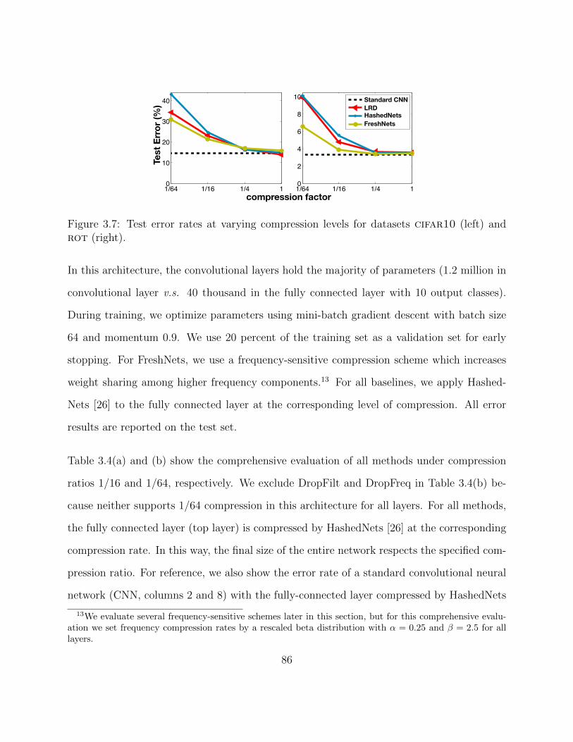
1/64 1/16 1/4 10

10

20

30

40

1/64 1/16 1/4 10

2

4

6

8

10

Standard CNNLRDHashedNetsfreshCNN

compression factor

Test

Err

or (%

) Standard CNNLRDHashedNetsFreshNets

Figure 3.7: Test error rates at varying compression levels for datasets cifar10 (left) androt (right).

In this architecture, the convolutional layers hold the majority of parameters (1.2 million in

convolutional layer v.s. 40 thousand in the fully connected layer with 10 output classes).

During training, we optimize parameters using mini-batch gradient descent with batch size

64 and momentum 0.9. We use 20 percent of the training set as a validation set for early

stopping. For FreshNets, we use a frequency-sensitive compression scheme which increases

weight sharing among higher frequency components.13 For all baselines, we apply Hashed-

Nets [26] to the fully connected layer at the corresponding level of compression. All error

results are reported on the test set.

Table 3.4(a) and (b) show the comprehensive evaluation of all methods under compression

ratios 1/16 and 1/64, respectively. We exclude DropFilt and DropFreq in Table 3.4(b) be-

cause neither supports 1/64 compression in this architecture for all layers. For all methods,

the fully connected layer (top layer) is compressed by HashedNets [26] at the corresponding

compression rate. In this way, the final size of the entire network respects the specified com-

pression ratio. For reference, we also show the error rate of a standard convolutional neural

network (CNN, columns 2 and 8) with the fully-connected layer compressed by HashedNets

13We evaluate several frequency-sensitive schemes later in this section, but for this comprehensive evalu-ation we set frequency compression rates by a rescaled beta distribution with α = 0.25 and β = 2.5 for alllayers.

86

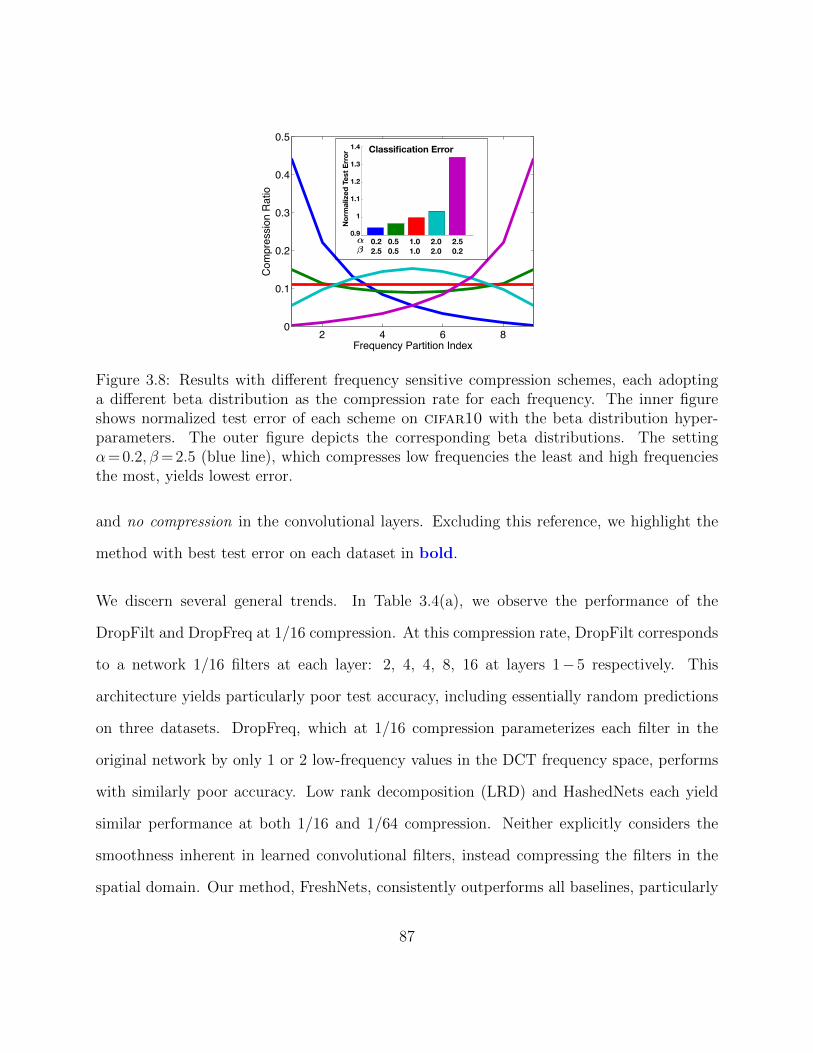
2 4 6 80

0.1

0.2

0.3

0.4

0.5

Frequency Partition Index

Com

pres

sion

Rat

io

alpha=0.2; beta=2.5; err=0.94alpha=0.5; beta=0.5; err=0.97alpha=1.0; beta=1.0; err=1.00alpha=2.0; beta=2.0; err=1.04alpha=2.5; beta=0.2; err=1.34

1 2 3 4 50.9

1

1.1

1.2

1.3

1.4

Nor

mal

ized

Tes

t Erro

r

�↵

Nor

mal

ized

Tes

t Err

or

0.2 0.5 1.0 2.0 2.52.5 0.5 1.0 2.0 0.2

Classification Error

0.9

1

1.1

1.2

1.3

1.4

Figure 3.8: Results with different frequency sensitive compression schemes, each adoptinga different beta distribution as the compression rate for each frequency. The inner figureshows normalized test error of each scheme on cifar10 with the beta distribution hyper-parameters. The outer figure depicts the corresponding beta distributions. The settingα= 0.2, β= 2.5 (blue line), which compresses low frequencies the least and high frequenciesthe most, yields lowest error.

and no compression in the convolutional layers. Excluding this reference, we highlight the

method with best test error on each dataset in bold.

We discern several general trends. In Table 3.4(a), we observe the performance of the

DropFilt and DropFreq at 1/16 compression. At this compression rate, DropFilt corresponds

to a network 1/16 filters at each layer: 2, 4, 4, 8, 16 at layers 1−5 respectively. This

architecture yields particularly poor test accuracy, including essentially random predictions

on three datasets. DropFreq, which at 1/16 compression parameterizes each filter in the

original network by only 1 or 2 low-frequency values in the DCT frequency space, performs

with similarly poor accuracy. Low rank decomposition (LRD) and HashedNets each yield

similar performance at both 1/16 and 1/64 compression. Neither explicitly considers the

smoothness inherent in learned convolutional filters, instead compressing the filters in the

spatial domain. Our method, FreshNets, consistently outperforms all baselines, particularly

87

at the higher compression rate as shown in Table 3.4(b). Using the same model in Table 3.3,

Figure 3.7 shows more complete curves of test errors with multiple compression factors on

the cifar10 and rot datasets.

Varying compression by frequency. As mentioned in Section 3.2.3, we allow a higher

collision rate in the high frequency components than in the low frequency components for

each filter. To demonstrate the utility of this scheme, we evaluate several hash compression

schemes. Systematically, we set the compression rate of the jth frequency band rj with a

parameterized function, i.e. rj = f(j). In this experiment, we use the beta distribution:

f(j;α, β) = Zxα−1(1 − x)β−1, where x = j+12k−1 is a real number between 0 and 1, k is the

filter size, and Z is a normalizing factor such that the resulting distribution of parameters

meets the target parameter budget K, i.e.∑2k−2

j=0 rjNj = K. We adjust α and β to control

the compression rate for each frequency region. As shown in Figure 3.8, we have multiple

pairs of α and β, each of which results in a different compression scheme. For example,

if α = 0.25 and β = 2.5, the compression rate monotonically decreases as a function of

component frequency, meaning more parameter sharing among high frequency components

(blue curve in Figure 3.8).

To quickly evaluate the performance of each scheme, we use a simple four-layer FreshNets

where the first two layers are DCT-hashed convolutional layers (with 5×5 filters) containing

32 and 64 feature maps respectively, and the last two layers are fully connected layers. We

test FreshNets on cifar10 with each of the compression schemes shown in Figure 3.8. In

each, weight sharing is limited to be within groups of similar frequencies, as described in

Section 3.2.3, however number of unique weights shared within each group is varied. We

denote the compression scheme with α, β = 1 (red curve) as a frequency-oblivious scheme

88

(a) Standard CNN (c) HashedNets (b) FreshNets

Figure 3.9: Visualization of filters learning on mnist in (a) an uncompressed CNN, (b) aCNN compressed with FreshNets, and (c) a CNN compressed with HashedNets (compressionrate 1/16 in both (b) and (c)). FreshNets preserves the smoothness of the filters, whereasHashedNets does not.

since it produces a uniform compression independent of frequency. In the inset bar plot in

Figure 3.8, we report test error normalized by the test error of the frequency-oblivious scheme

and averaged over compression rates 1, 1/2, 1/4, 1/16, 1/64, and 1/256. We can see that the

proposed scheme with fewer shared weights allocated to high frequency components (repre-

sented by the blue curve) outperforms all other compression schemes. An inverse scheme

where the high frequency regions have the lowest collision rate (purple curve) performs the

worst. These empirical results fit our assumption that the low frequency components of a

filter are more important than the high frequency components.

Filter visualization. We investigate the smoothness of the learned convolutional filters in

Figure 3.9 by visualizing the filter weights (first layer) of (a) a standard, uncompressed CNN,

(b) FreshNets, and (c) HashedNets (with weight sharing in the spatial domain). For this

experiment, we again apply a four layer network with two convolutional layers but adopt

larger filters (11 × 11) for better visualization. All three networks are trained on mnist,

and both FreshNets and HashedNets have 1/16 compression on the first convolutional layer.

When plotting, we scale the values in each filter matrix to the range [0, 255]. Hence, white

and black pixels stand for large positive and negative weights, respectively. We observe that,

89

although more blurry due to the compression, the filter weights of FreshNets are still smooth

while weights in HashedNets appear more chaotic.

3.2.6 Conclusion

In this chapter we have presented FreshNets, a method for learning convolutional neural

networks with dramatically compressed model storage. Harnessing the hashing trick for

parameter-free random weight sharing and leveraging the smoothness inherent in convolu-

tional filters, FreshNets compresses parameters in a frequency-sensitive fashion such that

significant model parameters (e.g. low-frequency components) are better preserved. As

such, FreshNets preserves prediction accuracy significantly better than competing baselines

at high compression rates.

90

Chapter 4

Deep learning Meets Embedding:

An Application to Model

Compression

In previous chapters, we have discussed model compression for deep learning models as well

as the embedding method for compressing heuristics. In this chapter, we combine the topics

of deep learning and embedding, and introduce neural networks with category embedding

tailored for traditional data mining tasks in which the one-hot encoding is widely used for

converting categorical features to numerical features. We show that a naıve use of one-

hot encoding might result in great memory consumption, as the weight matrix in the first

layer can be gigantic when many categories are present. We demonstrate that, similar to

the technique of low-rank decomposition described in Chapter 3, the category embedding is

equivalent to factorizing the weight matrix induced by the classic one-hot encoding, leading

to great memory savings. We further compress the embedding matrix with the hashing

trick discussed in Chapter 3. Our method is highly inspired by word embedding [5] and the

CBOW model [95]. The novelty is that we demonstrate the visualization of the embeddings

91

of categories provides certain degree of interpretability, which is critical for data mining

tasks. In particular, similar categories are mapped to nearby regions in the embedding

space. At the beginning of this chapter, we first switch our attention to the pros and cons of

using neural network in traditional data mining task to motivate category embedding. We

discuss its compression property in Section 4.3.1. At the end, we provide surprisingly good

visualization and clustering for categorical features.

4.1 Introduction

Deep neural networks and their variants have become the gold standard for a broad range

of applications as we can see in Chapter 3. There are many reasons contributing to the

recent success of neural networks in machine learning communities. The most important

reason, arguably, is that neural network itself has superior expressive power. According to

the universal approximation theorem [65], a multi-layer feed-forward neural neural network

is capable of approximating any measurable functions to any desired degree of accuracy.

However, can we get to that “perfect” neural net? There have been a longstanding con-

ventional wisdom that the function surfaces of neural networks contain a large amount of

local minima until Dauphin et al. [37] argue that they are in fact just critical points most of

which are actually saddle points. With proper training such as stochastic gradient descent,

we can escape from those saddle points [49]. Also, the emergence of training techniques such

as Adagrad [43] and dropout [133] further improve the practical performance of neural net-

works. Another key reason is the increasing availability of big datasets which enable neural

networks to absorb sufficient amount of data for parameter learning. Meanwhile, the use

of GPU dramatically speeds up the computation within neural networks by several orders

92

of magnitude compared with traditional multi-thread CPU computing, allowing neural net-

works to take in more data inputs given the same amount of training time and consequently

leading to better generalization performance.

However, compared to its success in AI applications such as computer vision and speech

recognition, neural networks seem not graining as much popularity as it should be in tradi-

tional data mining tasks. As opposed to computer vision where the input data are all “raw”

features of same type (e.g. pixels), traditional data mining tasks typically contain many fea-

tures generated from multiple sources (e.g. gender, country, height, education background,

and etc). For these problems, traditional algorithms such as logistic regression, SVM or tree

emsembles are still in favor. However, they all have their downsides. Logistic regression

is a linear model which limits the expressive power. SVM with kernel is non-parametric

and thus the number of support vectors might grow fast for large-scale datasets. Its online

training is also a big hassle. Tree ensembles like random forest and gradient boosting trees

are not good at handling sparse data, and their generalization ability is unstable when the

test instance goes beyond the region of training set. In contrast, neural networks do not have

those problems and offer much better expressive power. In fact, SVM and tree emsembles

may need an exponentially large number of training examples to get the same generalization

error as some deep neural networks [99].

Although neural networks have the above advantages, there are some special needs in tra-

ditional data mining tasks that standard neural networks have not addressed well. First,

hand-crafted features are usually a mix of numerical and categorical features, which poses a

challenge for directly applying neural networks as they can only deal with numerical inputs

by design. Second, the amount of categorical features keeps increasing in lots of applications.

93

In fact, in order to gain more nonlinearity, a trend is to make numerical features categor-

ical by binning or tree partition. Binning is a method to partition each numerical feature

with independent equal-size bins where each bin stands for a category. Third, to capture

high-order relationship between features, cross features are often used, which is a Cartesian

product of the category sets of all involved features, leading to exponentially growing num-

ber of categories. Another need by a data mining task is interpretability [35], the ability to

extract human-readable knowledge from the model. There have been some early attempts

trying to extract rules from trained neural networks [2, 85]. However, those rules are just a

proxy for neural networks rather than knowledge directly extracted from neural networks.

To address these problems, we advocate an end-to-end neural network architecture with

categorical feature embeddings. The model not only naturally handles both categorical and

numerical features, but also (and more importantly) visualizes feature similarity, which pro-

vides certain degree of interpretability. Our model is inspired by word embedding [5] and

the CBOW model [95], and therefore is by no means a brand-new method. For ease of pre-

sentation, we use the name “CENN” to denote this architecture throughout this chapter. In

particular, CENN has two branches to deal with numerical and categorical inputs, respec-

tively. Inspired by word embedding, the categorical branch is responsible for converting each

categorical feature to a numerical one by learning an embedding for each category of each

feature. These two branches are joined in the hidden layer and fed into the remaining feed-

forward neural network. Both the embeddings and the weights of CENN are jointly learned

through backpropagation. We further discuss the relationship between one-hot encoding and

CENN and how we can extend CENN to incorporate feature hashing [148]. With embed-

dings in place, we can directly plot the embeddings, which visualizes the feature similarity

found by CENN. Moreover, clustering of the embeddings yields unprecedented visualization

94

-0.1

2.1

0.4

1.6

2

4

1

-0.1

2.1

0.4

1.6

1.2

0.3

-1.1

-0.8

Identity Mapping

Sum

Retrive

SoftmaxOutput

Num

eric

al F

eatu

res

Cat

egor

ical

Fea

ture

s#hidden units

m = 5

Lookup Tablefor Embeddings U

WWeight matrix

Figure 4.1: The architecture of CENN for classification.

of feature categories. As in the case of word embedding, CENN maps similar categories to

nearby regions in the embedding space.

4.2 Method

Suppose we have a dataset {xi, yi}Ni=1 containing N instances, where xi and yi are the feature

vector and label of instance i, respectively. Each feature vector is a concatenation of two

parts, numerical features xRi and categorical features xCi . Each element in xRi is numerical

and each element of xCi is ordinal. CENN first converts the categorical part to a numerical

hidden representation which is then concatenated with the original numerical part. This

new representation will be fed into the remaining neural network and generate the final

output. Figure 4.1 shows the general architecture of CENN for classification purpose. Next,

we discuss the detail of each part in the architecture.

95

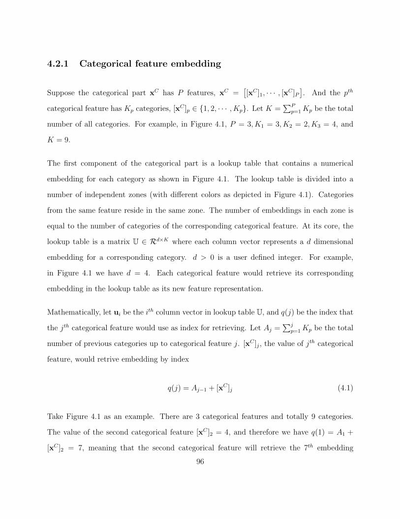
4.2.1 Categorical feature embedding

Suppose the categorical part xC has P features, xC =[[xC ]1, · · · , [xC ]P

]. And the pth

categorical feature has Kp categories, [xC ]p ∈ {1, 2, · · · , Kp}. Let K =∑P

p=1Kp be the total

number of all categories. For example, in Figure 4.1, P = 3, K1 = 3, K2 = 2, K3 = 4, and

K = 9.

The first component of the categorical part is a lookup table that contains a numerical

embedding for each category as shown in Figure 4.1. The lookup table is divided into a

number of independent zones (with different colors as depicted in Figure 4.1). Categories

from the same feature reside in the same zone. The number of embeddings in each zone is

equal to the number of categories of the corresponding categorical feature. At its core, the

lookup table is a matrix U ∈ Rd×K where each column vector represents a d dimensional

embedding for a corresponding category. d > 0 is a user defined integer. For example,

in Figure 4.1 we have d = 4. Each categorical feature would retrieve its corresponding

embedding in the lookup table as its new feature representation.

Mathematically, let ui be the ith column vector in lookup table U, and q(j) be the index that

the jth categorical feature would use as index for retrieving. Let Aj =∑j

p=1Kp be the total

number of previous categories up to categorical feature j. [xC ]j, the value of jth categorical

feature, would retrive embedding by index

q(j) = Aj−1 + [xC ]j (4.1)

Take Figure 4.1 as an example. There are 3 categorical features and totally 9 categories.

The value of the second categorical feature [xC ]2 = 4, and therefore we have q(1) = A1 +

[xC ]2 = 7, meaning that the second categorical feature will retrieve the 7th embedding

96

in the lookup table U as shown in Figure 4.1. After embedding retrieval, we obtain P

number of d dimensional embeddings. Similar to the summation in CBOW [95], we do an

element-wise summation to get the representation of all categorical features. Suppose the

new representation for categorical features is g(xC). Then we have

g(xC) =P∑j=1

uq(j) (4.2)

This new representation would then be fed into the next layer in the neural networks, and

all the embeddings are learned through back propagation.

4.2.2 Remaining layers

After obtaining the embedding for categorical features g(xC), CENN concatenates g(xC)

and the original numerical features xR to form a new representation for the original input

x. Suppose h` is the vector of hidden units in the layer `. The first hidden layer h1 =(g(xC),xR

). For the following layers, we have

h`+1 = σ(W`h` + b`) (4.3)

where W` and b` are the weight matrix and the bias vector for layer `, respectively. σ is

an activation function to make each layer a non-linear transformation. Possible activation

functions include rectifier linear units (ReLU) [51], sigmoid or tanh function. Note that

Figure 4.1 only shows two hidden layers for ease of illustration. However, one can use as

many hidden layers as necessary. For classification tasks, the final output layer is a softmax

function which estimates the probability of the given input belonging to each class. Thus,

97

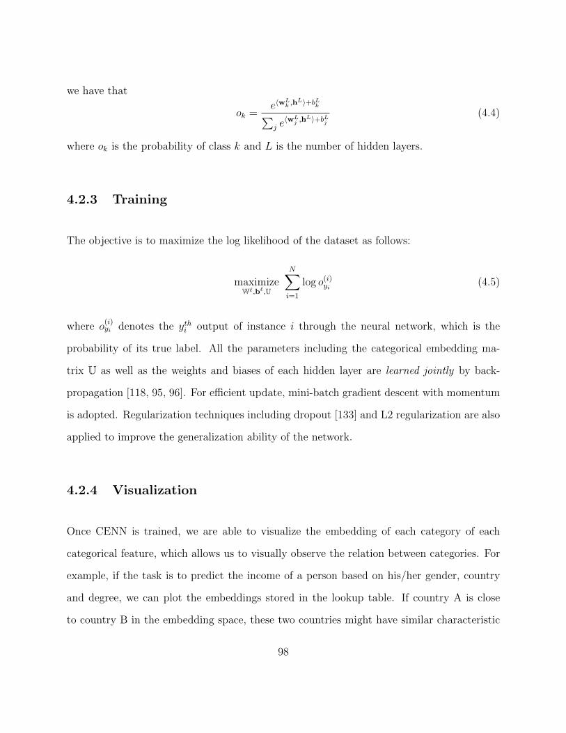
we have that

ok =e〈w

Lk ,h

L〉+bLk∑j e〈wL

j ,hL〉+bLj

(4.4)

where ok is the probability of class k and L is the number of hidden layers.

4.2.3 Training

The objective is to maximize the log likelihood of the dataset as follows:

maximizeW`,b`,U

N∑i=1

log o(i)yi (4.5)

where o(i)yi denotes the ythi output of instance i through the neural network, which is the

probability of its true label. All the parameters including the categorical embedding ma-

trix U as well as the weights and biases of each hidden layer are learned jointly by back-

propagation [118, 95, 96]. For efficient update, mini-batch gradient descent with momentum

is adopted. Regularization techniques including dropout [133] and L2 regularization are also

applied to improve the generalization ability of the network.

4.2.4 Visualization

Once CENN is trained, we are able to visualize the embedding of each category of each

categorical feature, which allows us to visually observe the relation between categories. For

example, if the task is to predict the income of a person based on his/her gender, country

and degree, we can plot the embeddings stored in the lookup table. If country A is close

to country B in the embedding space, these two countries might have similar characteristic

98

with respect to income. This visual information is important to interpret the model and

provides valuable insights. In addition, it is different from traditional visualization scenarios

where the visualized objects are instances rather than features in our case.

A naıve way to visualize the embeddings in the lookup table is to set the dimensionality of

embeddings to two or three. Once the training is done, we can directly plot the embedding

in a 2-D or 3-D space. Another way is to keep the dimensionality as is, which may be high-

dimensional. Then we can use off-the-shelf visualization methods such as t-SNE [138] for

the plot.

4.3 Discussion

We discuss some appealing properties of CENN in this section.

4.3.1 Compressing one-hot encoding

One-hot encoding is the most popular way to convert a categorical feature to a numerical

one. The new representation is a vector with one element being one and all others being

zero. For example, a feature with three categories (e.g. red, blue and green) would be

encoded as (1, 0, 0), (0, 1, 0) and (0, 0, 1). We show that the embeddings in CENN is a

matrix factorization of the weight matrix associated with one-hot encoding. For ease of

explanation, let’s assume there is no numerical features. The proof and conclusion still

apply in the presence of numerical features.

99

Let h be the vector of units in the hidden layer right after the lookup table and before

the activation function, and there are m hidden units in that layer. We use NN-onehot

to denote the neural network applying one-hot encoding to transform categorical features,

where the first hidden layer still contains m hidden units. In NN-onehot, Let V ∈ Rm×K

be the weight matrix of the first layer where K is the total number of categories of all

features. Note that K is also the length of the feature vector after one-hot encoding. In

CENN, let U ∈ Rd×K and W ∈ Rm×d be the embedding matrix and weight matrix as shown

in Figure 4.1 (assuming there is no numerical feature). Similar to [39], CENN is a direct

application of matrix decomposition on the first layer of NN-onehot.

Theorem 1 The category embeddings and their associated weight matrix in CENN is a

low-rank matrix decomposition of the weight matrix in NN-onehot, i.e. V = WU.

The proof is quite straightforward. Suppose r ∈ RK is the numerical vector converted from

xC with one-hot encoding scheme. Note that the indexing scheme in Eq. (4.1) is consistent

with the one-hot encoding. Hence, rj = 1 when j ∈ {q(p)|p = 1, · · · , P}, and rj = 0

otherwise. In NN-onehot, the hidden layer before activation is a linear transformation of

r as h = Vr. If we decompose V into W and U, we have h = WUr. For CENN, U is

the embedding matrix, and we can see that the representation for categorical features in

CENN is g(xC) =∑P

j=1 uq(j) = Ur according to Eq. (4.2). We illustrate this equation in

Figure 4.2 which is consistent with the example in Figure 4.1. Therefore, in CENN we have

h = Wg(xC) = WUr, which is equivalent to NN-onehot.

With Theorem 1, one can always convert NN-onehot to CENN by having an intermediate

hidden layer (between the input layer and the first hidden layer) that contains d number of

hidden units without activation function, where the weight matrix between the input and

100

1 2 3 4 5 6 7 8 9

010000110

872

U

r

Embedding matrix

one-hot encoding

at CENNg(xC)

Figure 4.2: One-hot encoding, mathematically Ur, is equivalent to the transformation per-formed in CENN that retrieves embeddings and does element-wise sum.

intermediate layer is U, and the weight matrix between the intermediate and the first hidden

layer is W [39].

Moreover, we have the following remarks about the comparison between CENN and one-hot

encoding:

• CENN is compact and exploits the low-rank structure of one-hot encoding in neural

networks thanks to matrix decomposition [39]. The memory footprint of the weight

matrix in one-hot encoding is mK, while CENN takes Kd for the lookup table and

md for the weight matrix, leading to d(K+m) footprint in total. Depending on tasks,

both K and m could be extremely large. For example, for industrial advertisement

prediction, the total number of categories could be at the scale of millions [92, 60].

With CENN, one can smoothly control the memory footprint by adjusting d, the

dimensionality of embeddings.

• With a more compact model, CENN does not necessarily lose generalization ability

compared with one-hot encoding. As demonstrated in Chapter 3, there has been a

general consensus that neural networks have certain degree of redundancy [26, 39, 64,

57, 27]. Denil et al. [39] show that matrix decomposition, which is what categorical

101

embedding in CENN is reduced to according to Theorem 1, can effectively preserve

the accuracy performance while reducing the size of a neural network.

From the discussion above, we can see that CENN can achieve superior tradeoff between

model size, efficiency and generalization ability, and adjust it by simply adjusting the di-

mensionality of embeddings.

4.3.2 Feature hashing for CENN

Typically, one-hot encoding results in high-dimensional sparse vectors, and thus is often

followed by feature hashing [148, 128, 36] as discussed in Chapter 3. Feature hashing has

been previously studied as a technique for reducing model size and speeding up learning, and

has been widely deployed in modern machine learning systems, such as vowpal wabbit [1].

In general, it can be regarded as a dimensionality reduction method which maps an input

vector x ∈ RK to a much smaller feature space via a mapping φ :RK → RD where D � K.

The mapping function φ consists of two approximately uniform auxiliary hash functions

h :N → {1, . . . , D} and ξ :N → {−1,+1}. The jth element of the D-dimensional hashed

input is defined as

φj(x) =∑

i:h(i)=j

ξ(i) xi. (4.6)

The dimensionality reduction comes at a price of collisions incurred by hashing, where mul-

tiple features are mapped into the same dimension. This problem is less severe for sparse

data sets, which is why feature hashing is a good fit for one-hot encoding.

102

We now show CENN can readily incorporate feature hashing. Let r still be the one-hot

encoded feature vector. After feature hashing, the ith element of the hashed vectors is

φi(r) =K∑

j:h(j)=i

ξ(j)rj =P∑

p:h(q(p))=i

ξ(j) (4.7)

where the first equality is a rewrite of Eq. (4.6), and the second equality holds because rj = 1

only when j ∈ {q(p)|p = 1, · · · , P} and rj = 0 otherwise. The hidden layer is still a linear

transformation of hashed input:

h = Vhφ(r) (4.8)

where Vh ∈ Rm×D is the weight matrix.

CENN can be extended to incorporate feature hashing by simply making the indexing func-

tion in Eq. (4.1) a hash function. To avoid confusion, we use qh as the new indexing function,

and q still keeps its definition in Eq. (4.1). As stated in Theorem 1, we can decompose

Vh = WUh where W ∈ Rm×d is still the weight matrix in CENN and Uh ∈ Rd×D is the new

lookup table with D number of d-dimensional embeddings. Following Eq. (4.8), we have

that h = WUhφ(r). Let the new representation after lookup table be gh(xC) = Uhφ(r), we

have that

gh(xC) = Uhφ(r) =

P∑p=1

ξ(q(p))uh(q(p)) (4.9)

=P∑p=1

ξh(p)uqh(p) (4.10)

where qh(·) = h(q(·)) and ξh(·) = ξ(q(·)) are the hash functions for CENN.

In summary, CENN can seamlessly incorporate feature hashing by the following three steps:

103

• Change the number of embeddings in lookup table from K to D.

• Change the indexing function of lookup table from q to qh.

• After the embeddings are retrieved, do element-wise summation up to a sign factor ξh

according to Eq. (4.10).

With feature hashing, different categories share the same embedding when they are mapped

to the same bucket by the hash function, which further reduces the size of the lookup table.

4.3.3 Dimensionality of embeddings

The dimensionality of the embeddings d in the lookup table is an important factor in CENN.

As discussed in Section 4.3.1, d is a tradeoff between model size, efficiency and the represen-

tation power of CENN. Here, one reluctant assumption CENN makes is that all embeddings

share the same dimensionality, which may not be realistic for some tasks and does not ac-

curately reflect each category’s representation complexity. For example, a feature with 100

categories may need a larger d to capture all information than one with only 3 categories.

One way to address this problem is to group features of similar number of categories and

have a separate lookup table for each group. Then we can independently adjust the dimen-

sionality of each lookup table. However, this might introduce a lot of ad-hoc work for each

task as well as overhead of keeping multiple lookup tables. Besides, for some tasks, the vast

majority of categories are rarely used [92]. A feature with many categories may not deserve

a higher dimensional lookup table. Feature hashing described in Section 4.3.2 may alleviate

this problem by sharing embedding between frequent categories and rare categories. Another

interesting idea is to have variable-length embedding for each category, which was recently

104

introduced by [101]. It introduces a latent variable z for each embedding that represents the

dimensionality which is learned jointly with the embedding. This would allow the data to

speak for themselves and automatically determine the dimensionality of the embedding of

each category.

4.3.4 Relation to factorization machines

Factorization machine (FM) [112, 113] is a general approach to model the interaction be-

tween categorical features, and has been used in many applications such as recommender

systems [115]. The model prediction, given a feature vector, is defined as

y(r) = w0 +n∑i=1

wiri +n∑i=1

n∑j=i+1

〈vi,vj〉rirj (4.11)

where r is a sparse high-dimensional feature vector generated by one-hot encoding, feature

engineering or discretization of numerica features. Usually, the value of each element of r is

either 0 or 1. Like CENN, FM also learns an embedding for each category (vi in Eq. (4.11))

and captures the interaction between two categories by the inner product of their embeddings.

CENN and FM are fundamentally different in the following three aspects.

• FM is a second-order function over the input r while CENN is a highly nonlinear

function with respect to r depending on the activation functions and the number of

layers in the neural network.

• FM models interaction by the inner product of embeddings. In contrast, CENN models

the interaction leveraging the nonlinearity of neural networks. Further, CENN can also

directly model the interaction by learning embeddings for cross features. Suppose two

105

features have category sets A and B, respectively. We can create a new feature whose

value is the Cartesian product of these two features, i.e. A×B. The embedding learned

for categories in the cross feature directly models the interaction between these two

features.

• FM cannot naturally handle multi-label classification as it only learns a single score

function. Current off-the-shelf packages [113] do not support multi-label classification

either. In contrast, CENN can naturally do multi-class classification with a softmax

output. Moreover, CENN does not require ad-hoc implementation because all of its

building blocks have been implemented by current deep learning packages, such as

Torch, Theano and etc. With these packages, it is also very easy to incorporate state-

of-the-art training techniques such as dropout [133] and Adagrad [43] in CENN with

only a few lines of code.

4.4 Related work

The CENN architecture is inspired by embedding-based modeling, especially the distributed

word representation for natural language processing (NLP) [5, 95, 96, 94, 21]. The goal of

language modeling is to estimate the probability of generating a particular sentence. With

the Markovian assumption, the probability of a word only hinges on its context, which can

be computed by the n-gram counting-based model [18]. However, its model complexity

increases dramatically as n gets large. To overcome this problem, Bengio et al. [5] proposed

to learn a representation for each word. The neural network can take the embedding of each

word in the context as input and make the prediction. Its biggest difference compared with

CENN is that it enforces different positions of the context to have exactly the same word

106

set, meaning that the same word embedding coud appear everywhere associated with the

input. In contrast, in CENN, different features possess different category sets which is more

suitable for traditional data mining tasks.

In addition to NLP, embedding-based methods also widely exist in recommender systems to

model pair-wise relationship. Lots of recommender systems are based on the classic user-

item patterns (e.g. user-movie, user-ads and image-tag) where the task is to estimate the

similarity score between users and items. It can be regarded as a classification/regression

problem with two categorical features: user ID and item ID. Each category of user ID and

item ID would be assigned an embedding, and their similarity is mostly modeled by the

inner product of their embeddings. A majority of collaborative filtering models fall into

this category, such as Wsabie [149] and SVD++ [69]. Further, tensor decomposition [114]

and factorization machines [112] are able to model the pair-wise interactions between more

categorical variables, and take side information into account with careful feature design.

CENN handles numerical and categorical features naturally which is vital to a wide range of

data mining tasks. In order to do this, CENN has two input branches dealing with numerical

and categorical features, respectively, each of which is independent from the other. This is

different than the siamese network [13, 28] where two branches share the same parameters. In

the literature, lots of traditional machine learning models require the input to be numerical,

such as SVM, logistic regression and vanilla neural networks, which all require a preprocessing

step to convert categorical features to numerical features, such as one-hot encoding [144].

Besides one-hot encoding, another transformation approach is mapping a category to the

conditional probability of a particular label given the category [24, 22, 62, 61].

Like CENN, tree-based methods are also able to handle both numerical and categorical

features. In particular, tree ensembles such as random forest [12], gradient boosting trees [45]

107

and adaboost [44] are usually preferred to alleviate potential issues of high bias or high

variance [58] introduced by a single tree. Recently He et al. introduces a machine learning

model [60] used by ads prediction at Facebook which combines a tree ensemble model with

the one-hot encoding. The basic idea is to first convert the input to a new categorical

feature vector using gradient boosting trees, and then use one-hot encoding to convert the

categorical feature vector back to a numerical feature vector and use logistic regression as the

final predictor. In contrast to the typical feature binning methods which partition the space

into equal-size grid, boosting trees are able to take the supervised label information into

account when partitioning the space, leading to better categorical features. This category

generating technique could be well suited for CENN as CENN is good at handling categorical

features.

As discussed in Section 4.3.1, CENN is essentially a compressed version of one-hot encoding,

leading to a more compact model with less overfitting. In Chapter 3, we have surveyed

several methods that try to attack the redundancy issue of neural nets. Denil et al. [39]

re-parameterize the weight matrix as the product of two smaller matrices, resulting in less

parameters as well as faster training and testing. CENN enjoys all its advantages since

CENN also utilizes the same matrix decomposition technique. Similar observation have

been made in the context of word embedding with the skip-gram model with negative-

sampling (SGNS). Specifically, SGNS is implicitly factorizing a word-context matrix where

each element is the point-wise mutual information of corresponding word and context [83].

Li et al. [84] further strengthen the statement that SGNS is an explicit matrix factorization

of the word co-occurrence matrix.

108

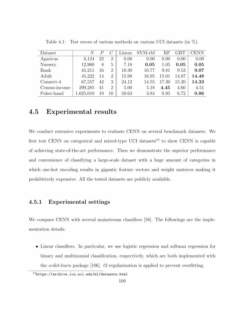
Table 4.1: Test errors of various methods on various UCI datasets (in %).

Dataset N P C Linear SVM-rbf RF GBT CENNAgaricus 8,124 22 2 0.00 0.00 0.00 0.00 0.00Nursery 12,960 8 5 7.18 0.05 1.05 0.05 0.05Bank 45,211 16 2 10.30 10.77 9.81 9.53 9.07Adult 45,222 14 2 15.98 16.95 15.01 14.87 14.48Connect-4 67,557 42 3 24.12 14.55 17.30 15.20 14.33Census-income 299,285 41 2 5.00 5.18 4.45 4.60 4.51Poker-hand 1,025,010 10 10 50.63 3.84 8.95 6.72 0.86

4.5 Experimental results

We conduct extensive experiments to evaluate CENN on several benchmark datasets. We

first test CENN on categorical and mixed-type UCI datasets14 to show CENN is capable

of achieving state-of-the-art performance. Then we demonstrate the superior performance

and convenience of classifying a large-scale dataset with a huge amount of categories in

which one-hot encoding results in gigantic feature vectors and weight matrices making it

prohibitively expensive. All the tested datasets are publicly available.

4.5.1 Experimental settings

We compare CENN with several mainstream classifiers [58]. The followings are the imple-

mentation details:

• Linear classifiers. In particular, we use logistic regression and softmax regression for

binary and multinomial classification, respectively, which are both implemented with

the scikit-learn package [106]. `2 regularization is applied to prevent overfitting.

14https://archive.ics.uci.edu/ml/datasets.html

109

• Support vector machines with RBF kernels (SVM-rbf) implemented by libSVM [16].

Its hyperparameters include kernel bandwidth and `2 regularization. In order for

SVM-rbf to run as fast as possible, we set the cache size of LibSVM to 10GB which is

sufficiently large for all the tested datasets.

• Random forest (RF). We adopt the implementation in the scikit-learn package [106].

The number of trees and the maximum depth of each tree are tuned via the validation

set.

• Gradient boosting trees (GBT). We adopt the xgboost package [19] which is currently

the state-of-the-art software for GBT. Early stopping is applied to prevent overfitting.

In particular, if the validation error does not get reduced for 100 rounds, GBT would

stop and the number of boosted trees would be the one that achieves the best validation

error. The maximum number of trees is set to 3000. The shrinkage factor and the

maximum depth of its tree is tuned via the validation set.

• CENN is implemented based on the Torch7 package [33] and runs on GPUs (NVIDA

GTX TITAN graphics cards). Models are trained via stochastic gradient descent.

For UCI datasets, a small batch size such as 5 is used for computing the gradient.

Momentum is always fixed at 0.5. The number of hidden units is 1000 for each hidden

layer. All other hyperparameters are tuned including the initial learning rate, decay

factor of learning rate, number of hidden layers, embedding size for CENN, dropout

and `2 regularization. Like GBT, early stopping is used to prevent overfitting. We use

rectifier linear units for all activation functions. In the experiments, we do not show

the result of standard neural network with one-hot encoding (NN-onehot), because

CENN is equivalent to NN-onehot with an intermediate layer that contains d number

110

of hidden units where d is the dimensionality of the embeddings, as discussed in the

Section 4.3.

The experiments are run on an off-the-shelve desktop with two 8-core Intel(R) Xeon(R)

processors of 2.67 GHz and 128GB RAM. For datasets in which the test set is not specified,

we split the dataset and use 2/3 for training and 1/3 for testing. We further hold out 1/3

from the training set as the validation set. All algorithms are trained on the training set,

choosing hyperparameters based on the validation set and evaluated on the test set. All our

reported results are based on the test error performance. Hyperparameters are selected for

all algorithms with Bayesian optimization [132], implemented in the spearmint15 package.

4.5.2 Evaluation on UCI datasets

We evaluate the performance of CENN on several UCI benchmark datasets as shown in

Table 4.1. We show the dataset statistics on the left part of the table and the test error

performance on the right part. Here, N , P and C stands for the number of instances, the

number of features and the number of classes in each dataset, respectively. The datasets are

ordered by N . We try to include datasets of different types, ranging from “easy” datasets

that can be perfectly classified such as Agaricus to “hard” ones for which linear models

are merely as good as random guess such as Poker-hand. Among all these datasets, Bank,

Adult and Census datasets contain both categorical feature and numerical features, while the

other datasets are all categorical datasets. We choose datasets with many categorical features

since they are the focus of CENN. From Table 4.1, we make the following observations. First,

linear classifiers perform the worst in most cases, especially on categorical datasets. Second,

15https://github.com/JasperSnoek/spearmint

111

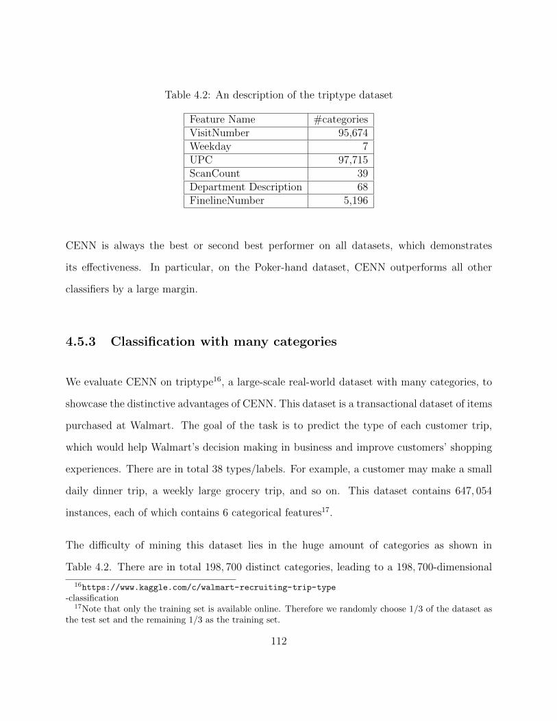
Table 4.2: An description of the triptype dataset

Feature Name #categoriesVisitNumber 95,674Weekday 7UPC 97,715ScanCount 39Department Description 68FinelineNumber 5,196

CENN is always the best or second best performer on all datasets, which demonstrates

its effectiveness. In particular, on the Poker-hand dataset, CENN outperforms all other

classifiers by a large margin.

4.5.3 Classification with many categories

We evaluate CENN on triptype16, a large-scale real-world dataset with many categories, to

showcase the distinctive advantages of CENN. This dataset is a transactional dataset of items

purchased at Walmart. The goal of the task is to predict the type of each customer trip,

which would help Walmart’s decision making in business and improve customers’ shopping

experiences. There are in total 38 types/labels. For example, a customer may make a small

daily dinner trip, a weekly large grocery trip, and so on. This dataset contains 647, 054

instances, each of which contains 6 categorical features17.

The difficulty of mining this dataset lies in the huge amount of categories as shown in

Table 4.2. There are in total 198, 700 distinct categories, leading to a 198, 700-dimensional

16https://www.kaggle.com/c/walmart-recruiting-trip-type

-classification17Note that only the training set is available online. Therefore we randomly choose 1/3 of the dataset as

the test set and the remaining 1/3 as the training set.

112

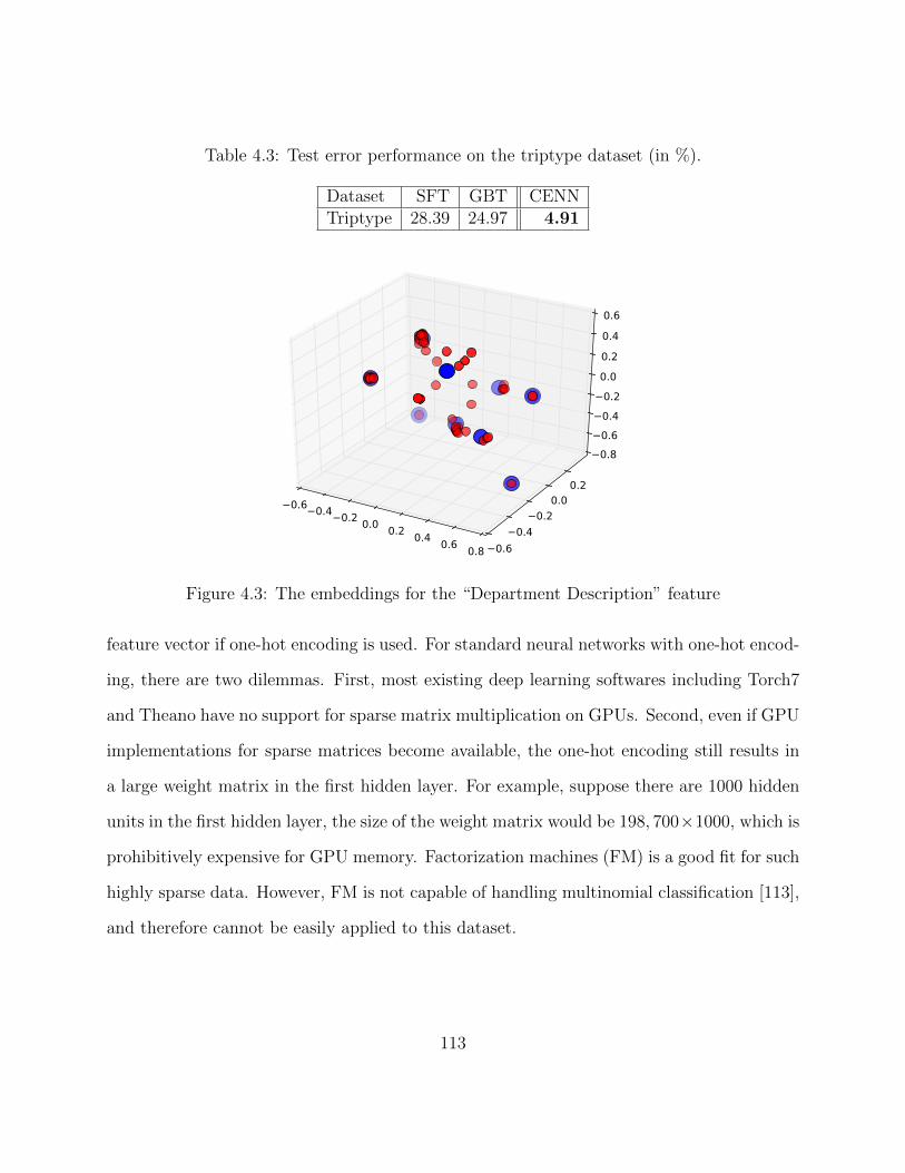
Table 4.3: Test error performance on the triptype dataset (in %).

Dataset SFT GBT CENNTriptype 28.39 24.97 4.91

Figure 4.3: The embeddings for the “Department Description” feature

feature vector if one-hot encoding is used. For standard neural networks with one-hot encod-

ing, there are two dilemmas. First, most existing deep learning softwares including Torch7

and Theano have no support for sparse matrix multiplication on GPUs. Second, even if GPU

implementations for sparse matrices become available, the one-hot encoding still results in

a large weight matrix in the first hidden layer. For example, suppose there are 1000 hidden

units in the first hidden layer, the size of the weight matrix would be 198, 700×1000, which is

prohibitively expensive for GPU memory. Factorization machines (FM) is a good fit for such

highly sparse data. However, FM is not capable of handling multinomial classification [113],

and therefore cannot be easily applied to this dataset.

113

Table 4.4: Results of k-means clustering on the learned embeddings in CENN.

Cluster Names of the categories1 shoes, boys wear, jewelry and sunglasses, mens wear, accessories, infant

consumable hardlines, ladieswear, sheer hosiery, wireless, infant apparel,ladies socks, plus and maternity, electronics, girls wear, 4-6x and 7-14, bras& shapewear, sleepwear/foundations, cameras and supplies, players andelectronics, menswear, swimwear/outerwear, media and gaming, 1-hr photo,health and beauty aids

2 paint and accessories, impulse merchandise, candy, tobacco, cookies, homemanagement, cook and dine, hardware, bedding, bath and shower, homedecor, liquor,wine,beer, other departments, furniture, seasonal, large house-hold goods

3 meat - fresh & frozen, dairy, pets and supplies, produce, grocery dry goods,frozen foods, service deli, pre packed deli, comm bread, bakery, seafood

4 fabrics and crafts, celebration, books and magazines, office supplies, toys,sporting goods, concept stores

5 household chemicals/supp, pharmacy otc, household paper goods, phar-macy rx, optical - frames, optical - lenses

6 automotive, lawn and garden, horticulture and access7 personal care, beauty8 dsd grocery9 financial services

We only show the results of softmax regression, GBT18 and CENN, since RF, SVM-rbf

are too slow to achieve any meaningful results on this dataset even with state-of-the-art

packages. For CENN, we adopt a deep structure with four hidden layers each of which

contains 1000 hidden units. We intentionally use the raw feature without any complicated

feature engineering, as that would introduce a number of additional factors which we want

to disambiguate as alternative factors for success. We show the test error performance of

each method on Table 4.3. We can clearly see that CENN outperforms other classifiers by

18We found GBT tends to underfit this dataset due to the huge amount of categories. In order for GBT toperform well, we use 10, 000 boosted trees and set the depth of each tree to 15, whose entire training processcosts around 22 hours with 12 CPU cores. The early stop is triggered at the 9092nd tree.

114

a huge margin, which with no doubt demonstrates the great advantage of using CENN on

datasets with many categories.

Regarding the good performance on this dataset, should we give credits to features with

many categories, including VisitNumber, UPC and FinelineNumber? As a sanity check,

we apply softmax regression on this dataset without these three features and get 64.95%

test error. The presence of FinelineNumber help softmax regression reduce the test error to

63.72%. Likewise, CENN gets 63.22% test error with these three features removed. However,

softmax and CENN obtain 28.39% and 4.91% test errors, respectively, with the full dataset

as we can see from Table 4.3. This analysis strongly indicates the importance of VisitNumber

and UPC.

4.5.4 Visualization

We demonstrate the visualization ability of CENN on the triptype dataset and show that

the learned embeddings are surprisingly appealing according to the clustering result. We

set the embedding dimensionality to 3 and train CENN from scratch, which obtains 7.99%

test error at the end. Next, we plot the categories using their embeddings as coordinates.

Due to space limit and the fact that the “Department Description” is the only feature whose

semantic meaning of each category is released, we only present the visualization of this fea-

ture which contains 68 categories as shown in Figure 4.3. From this figure in which each

red point corresponds to a category, we can observe that there are some clustering struc-

tures. Therefore, we use kmeans to cluster all these 68 categories into 9 clusters where the

similarity is measured by the Euclidean distance between their three-dimensional embed-

dings. The clustering centers are visualized as blue points in Figure 4.3. In addition, we

115

show the clustering results along with the semantic meaning of categories in each cluster

in Table 4.4 ordered by cluster size. The clustering structure is surprisingly meaningful.

For example, most categories in the 1st cluster are related to apparel; the 2nd cluster is

related to household goods; the 3rd cluster is all about food; the 5th cluster is about family

healthcare; the 6th cluster is related to horticulture. These results strongly indicate that

CENN learns meaningful embeddings, which helps extract knowledge from data and improve

interpretability of the model.

Importantly, this cannot be done with other classifiers as well as traditional visualization or

clustering techniques. In CENN, each visualized point is a category of a categorical feature

rather than a data instance. These cannot be visualized by unsupervised embedding models

such as tSNE since similarity between categories is not well defined without supervision.

Even with supervision information, traditional embedding models such as metric learning

algorithms are only capable of learning a metric on data instances rather than categories.

In contrast, CENN learns an embedding for each category from which we can get a clear

picture of category similarities as shown in Table 4.4.

4.6 Conclusions

Neural networks are very powerful, beating other classifiers when trained properly. But they

are not widely used for many data mining tasks due to its difficulty in handling categorical

features with many categories as well as lack of interpretability. We have advocated the use of

category embedding for data mining tasks. It offers enormous advantages for jointly handling

large-scale mixed-type data as well as providing supervised visualization and knowledge

extraction, which most mainstream classifiers do not offer. The category embeddings can

116

be regarded as a matrix decomposition of the weight matrix of a standard neural network

with the classic one-hot encoding. We have also discussed the extension for incorporating

feature hashing, which promotes embedding sharing among different categories. We have

conducted comprehensive experiments to evaluate the empirical performance. Neural nets

with category embedding not only achieves state-of-the-art performance on UCI datasets,

but also beats all other classifiers by a large margin on a large-scale real-world dataset that

contains a huge amount of categories. More importantly, the visualization and clustering of

the learned embeddings uncover clear and reliable semantic meanings, as similar categories

are mapped to nearby regions in the embedding space. In the future, we will explore these

semantic clustering for enhancing the interpretability of data mining.

117

Chapter 5

Conclusions

Machine learning keeps setting new records in various applications, accompanied by ever-

increasing model size. We identify that models with large memory consumption lie in two

areas: memory-based learning and deep learning.

For memory-based learning, we have focused on one of its most promising applications—

learning Euclidean heuristic with graph embedding, which is an effective method for com-

pressing pair-wise distance matrix. However, training the underlying MVU embeddings are

slow, dramatically limiting its usage. To address this efficiency issue, we have proposed

maximum variance correction (MVC) that scales up MVU training by several order of mag-

nitude, from 4000 states to 200, 000 states. Different than other large-scale graph embedding

algorithms (e.g gl-MVU [147, 150]), MVC preserves the local distance constraints without

which the resulting heuristics are not able to find the optimal search path in the graph.

Moreover, We propose the goal-oriented Euclidean heuristic (GOEH) to improve the search

quality by better exploiting the prior knowledge of the goal sets.

For deep learning, we have proposed HashedNets, an approach to randomly grouping pa-

rameters within neural network using a low-cost hashing function. In particular, parameters

118

within the same group share the same magnitude up to a sign factor. Plus, HashedNets are

general and modular, complementary to other compressing techniques such as Dark Knowl-

edge [64]. We have demonstrated HashedNets achieve much better accuracy performance

than other baselines such as low-rank decomposition [39]. Though the hashing trick could

also be directly applied to convolutional layers, it does not leverage the distinct feature of

the convolutional filters—local smoothness. To address this problem, we further propose

Frequency-Sensitive HashedNets (FreshNets) that compresses parameters in the frequency

domain of the convolutional filters. In particular, we compress more on high-frequency do-

main, which are less important due to the property of local smoothness. Our empirical

results show that FreshNets obtains superior performance and outperforms a number of

baseline methods such as HashedNets, especially when the compression rate is large.

Combining deep learning and embedding, we further propose neural networks with categor-

ical feature embedding (CENN) with focus on traditional data mining tasks. We show that

the traditional one-hot encoding results into great memory consumption in the presence of

a huge amount of categories. For example, if there are 10 categorical features each of which

contains 100, 000 categories, the converted feature vector after one-hot encoding would be

a 1, 000, 000-dimensional sparse vector. If there are 1, 000 hidden neurons in the first layer,

the one-hot encoding would lead to a weight matrix of size 1, 000, 000 × 1, 000 in the first

layer, which is prohibitively expensive for the GPU memory. CENN addresses this problem

by learning a d-dimensional embedding for each category to form a new numerical represen-

tation for the neural network where d is a hyper-parameter. In the previous example, the

memory cost of CENN is 1, 000, 000 × d + 1, 000 × d, which is a great memory saving. We

further demonstrate that CENN is equivalent to a low-rank decomposition [39] of the one-

hot encoding. CENN not only achieves state-of-the-art performance on several benchmark

datasets, but also provides visualization and interpretability on the category similarity.

119

We believe the scalability and compactness of machine learning models will become increas-

ingly important in the future, in part because of the trend of applications shifting towards

mobile and embedded devices. As future work we plan to further investigate model compres-

sion for neural networks. One particular direction of interest is to optimize HashedNets for

GPUs. GPUs are very fast (through parallel processing) but usually feature small on-board

memory [87]. We plan to investigate how to use HashedNets to fit larger networks onto the fi-

nite memory of GPUs. A specific challenge in this scenario is to avoid non-coalesced memory

accesses due to the pseudo-random hash functions—a sensitive issue for GPU architectures.

120

References

[1] Alekh Agarwal, Olivier Chapelle, Miroslav Dudık, and John Langford. A reliableeffective terascale linear learning system. The Journal of Machine Learning Research,15(1):1111–1133, 2014.

[2] Robert Andrews, Joachim Diederich, and Alan B Tickle. Survey and critique of tech-niques for extracting rules from trained artificial neural networks. Knowledge-basedsystems, 8(6):373–389, 1995.

[3] Jimmy Ba and Rich Caruana. Do deep nets really need to be deep? In NIPS, pages2654–2662, 2014.

[4] M. Belkin and P. Niyogi. Laplacian eigenmaps for dimensionality reduction and datarepresentation. Neural Computation, 15:1373–1396, 2002.

[5] Yoshua Bengio, Rejean Ducharme, Pascal Vincent, and Christian Janvin. A neuralprobabilistic language model. The Journal of Machine Learning Research, 3:1137–1155, 2003.

[6] Christopher M. Bishop. Neural Networks for Pattern Recognition. Oxford UniversityPress, Inc., 1995.

[7] P. Biswas and Y. Ye. Semidefinite programming for ad hoc wireless sensor networklocalization. In Proceedings of the 3rd international symposium on Information pro-cessing in sensor networks, IPSN ’04, pages 46–54, New York, NY, USA, 2004. ACM.ISBN 1-58113-846-6.

[8] J. Blitzer, K.Q. Weinberger, L. K. Saul, and F. C. N. Pereira. Hierarchical distributedrepresentations for statistical language modeling. In Advances in Neural and Informa-tion Processing Systems, volume 17, Cambridge, MA, 2005. MIT Press.

[9] B. Borchers. Csdp, ac library for semidefinite programming. Optimization Methodsand Software, 11(1-4):613–623, 1999.

[10] Y-lan Boureau, Yann L Cun, et al. Sparse feature learning for deep belief networks.In NIPS, pages 1185–1192, 2008.

[11] S. Boyd and L. Vandenberghe. Convex Optimization. Cambridge University Press,New York, NY, USA, 2004. ISBN 0521833787.

121

[12] L. Breiman. Random forests. Machine Learning, 45(1):5–32, 2001.

[13] Jane Bromley, James W Bentz, Leon Bottou, Isabelle Guyon, Yann LeCun, CliffMoore, Eduard Sackinger, and Roopak Shah. Signature verification using a siamesetime delay neural network. International Journal of Pattern Recognition and ArtificialIntelligence, 7(04):669–688, 1993.

[14] T Brosch and R Tam. Efficient training of convolutional deep belief networks in thefrequency domain for application to high-resolution 2d and 3d images. Neural Com-putation, 27(1):211–227, 2015.

[15] Cristian Bucilua, Rich Caruana, and Alexandru Niculescu-Mizil. Model compression.In KDD, 2006.

[16] Chih-Chung Chang and Chih-Jen Lin. LIBSVM: A library for support vector machines.ACM Transactions on Intelligent Systems and Technology, 2:27:1–27:27, 2011.

[17] Minmin Chen, Kilian Q. Weinberger, Fei Sha, and Yoshua Bengio. Marginalized de-noising auto-encoders for nonlinear representations. In ICML, pages 1476–1484, 2014.

[18] Stanley F Chen and Joshua Goodman. An empirical study of smoothing techniquesfor language modeling. Computer Speech & Language, 13(4):359–393, 1999.

[19] Tianqi Chen and Carlos Guestrin. Xgboost: Reliable large-scale tree boosting system.

[20] W. Chen, K. Weinberger, and Y. Chen. Maximum variance correction with applicationto A∗ search. In Proc. ICML, 2013.

[21] Welin Chen, David Grangier, and Michael Auli. Strategies for training large vocabularyneural language models. arXiv preprint arXiv:1512.04906, 2015.

[22] Wenlin Chen, Yixin Chen, Yi Mao, and Baolong Guo. Density-based logistic regression.In KDD, 2013.

[23] Wenlin Chen, Yixin Chen, Kilian Q Weinberger, Qiang Lu, and Xiaoping Chen. Goal-oriented euclidean heuristics with manifold learning. In AAAI, 2013.

[24] Wenlin Chen, Yixin Chen, and Kilian Q Weinberger. Fast flux discriminant for large-scale sparse nonlinear classification. In KDD, 2014.

[25] Wenlin Chen, Yixin Chen, and Kilian Q Weinberger. Filtered search for submodularmaximization with controllable approximation bounds. In AISTATS, 2015.

[26] Wenlin Chen, James T Wilson, Stephen Tyree, Kilian Q Weinberger, and Yixin Chen.Compressing neural networks with the hashing trick. In ICML, 2015.

122

[27] Wenlin Chen, James T Wilson, Stephen Tyree, Kilian Q Weinberger, and Yixin Chen.Compressing convolutional neural networks. arXiv preprint arXiv:1506.04449, 2015.

[28] Sumit Chopra, Raia Hadsell, and Yann LeCun. Learning a similarity metric discrimi-natively, with application to face verification. In CVPR, 2005.

[29] Byung-Gon Chun and Petros Maniatis. Augmented smartphone applications throughclone cloud execution. In HotOS, 2009.

[30] Dan C Ciresan, Ueli Meier, Jonathan Masci, Luca M Gambardella, and Jurgen Schmid-huber. High-performance neural networks for visual object classification. arXiv preprintarXiv:1102.0183, 2011.

[31] Adam Coates, Andrew Y Ng, and Honglak Lee. An analysis of single-layer networksin unsupervised feature learning. In AISTATS, 2011.

[32] Adam Coates, Brody Huval, Tao Wang, David Wu, Bryan Catanzaro, and Ng An-drew. Deep learning with cots hpc systems. In Proceedings of The 30th InternationalConference on Machine Learning, pages 1337–1345, 2013.

[33] Ronan Collobert, Koray Kavukcuoglu, and Clement Farabet. Torch7: A matlab-likeenvironment for machine learning. In BigLearn, NIPS Workshop, 2011.

[34] M. Courbariaux, Y. Bengio, and J.-P. David. Low precision storage for deep learning.arXiv preprint arXiv:1412.7024, 2014.

[35] Zhicheng Cui, Wenlin Chen, Yujie He, and Yixin Chen. Optimal action extraction forrandom forests and boosted trees. In Proceedings of the 21th ACM SIGKDD Inter-national Conference on Knowledge Discovery and Data Mining, pages 179–188. ACM,2015.

[36] Anirban Dasgupta, Ravi Kumar, and Tamas Sarlos. A sparse johnson: Lindenstrausstransform. In Proceedings of the forty-second ACM symposium on Theory of computing,pages 341–350. ACM, 2010.

[37] Yann N Dauphin, Razvan Pascanu, Caglar Gulcehre, Kyunghyun Cho, Surya Gan-guli, and Yoshua Bengio. Identifying and attacking the saddle point problem in high-dimensional non-convex optimization. In NIPS, 2014.

[38] Jia Deng, Wei Dong, Richard Socher, Li-Jia Li, Kai Li, and Li Fei-Fei. Imagenet: Alarge-scale hierarchical image database. In Computer Vision and Pattern Recognition,2009. CVPR 2009. IEEE Conference on, pages 248–255. IEEE, 2009.

[39] Misha Denil, Babak Shakibi, Laurent Dinh, Nando de Freitas, et al. Predicting pa-rameters in deep learning. In NIPS, 2013.

123

[40] Emily L Denton, Wojciech Zaremba, Joan Bruna, Yann LeCun, and Rob Fergus.Exploiting linear structure within convolutional networks for efficient evaluation. InAdvances in Neural Information Processing Systems, pages 1269–1277, 2014.

[41] Jeff Donahue, Yangqing Jia, Oriol Vinyals, Judy Hoffman, Ning Zhang, Eric Tzeng,and Trevor Darrell. Decaf: A deep convolutional activation feature for generic visualrecognition. arXiv preprint arXiv:1310.1531, 2013.

[42] D.L. Donoho and C. Grimes. When does isomap recover the natural parameterizationof families of articulated images? Department of Statistics, Stanford University, 2002.

[43] John Duchi, Elad Hazan, and Yoram Singer. Adaptive subgradient methods for onlinelearning and stochastic optimization. The Journal of Machine Learning Research, 12:2121–2159, 2011.

[44] Yoav Freund and Robert E Schapire. A decision-theoretic generalization of on-linelearning and an application to boosting. Journal of computer and system sciences, 55(1):119–139, 1997.

[45] Jerome H Friedman. Greedy function approximation: a gradient boosting machine.Annals of statistics, pages 1189–1232, 2001.

[46] Kunihiko Fukushima. Neocognitron: A self-organizing neural network model for amechanism of pattern recognition unaffected by shift in position. Biological cybernetics,36(4):193–202, 1980.

[47] Kuzman Ganchev and Mark Dredze. Small statistical models by random feature mix-ing. In Workshop on Mobile NLP at ACL, 2008.

[48] Jacob Gardner, Matt Kusner, Kilian Weinberger, John Cunningham, et al. Bayesianoptimization with inequality constraints. In ICML, 2014.

[49] Rong Ge, Furong Huang, Chi Jin, and Yang Yuan. Escaping from saddle points—online stochastic gradient for tensor decomposition. arXiv preprint arXiv:1503.02101,2015.

[50] Ross Girshick, Jeff Donahue, Trevor Darrell, and Jitendra Malik. Rich feature hierar-chies for accurate object detection and semantic segmentation. In CVPR, 2014.

[51] Xavier Glorot, Antoine Bordes, and Yoshua Bengio. Deep sparse rectifier networks. InAISTATS, 2011.

[52] Xavier Glorot, Antoine Bordes, and Yoshua Bengio. Domain adaptation for large-scalesentiment classification: A deep learning approach. In ICML, pages 513–520, 2011.

124

[53] Yunchao Gong, Liu Liu, Ming Yang, and Lubomir Bourdev. Compressing deep con-volutional networks using vector quantization. arXiv preprint arXiv:1412.6115, 2014.

[54] Alex Graves, A-R Mohamed, and Geoffrey Hinton. Speech recognition with deeprecurrent neural networks. In ICASSP, 2013.

[55] N. Gupta and D.S. Nau. On the complexity of blocks-world planning. Artificial Intel-ligence, 56(2):223–254, 1992.

[56] Suyog Gupta, Ankur Agrawal, Kailash Gopalakrishnan, and Pritish Narayanan. Deeplearning with limited numerical precision. arXiv preprint arXiv:1502.02551, 2015.

[57] Song Han, Jeff Pool, John Tran, and William Dally. Learning both weights and con-nections for efficient neural network. In NIPS, 2015.

[58] Trevor. Hastie, Robert. Tibshirani, and JH (Jerome H.) Friedman. The elements ofstatistical learning. Springer, 2009.

[59] Kaiming He, Xiangyu Zhang, Shaoqing Ren, and Jian Sun. Delving deep into rectifiers:Surpassing human-level performance on imagenet classification. In Proceedings of theIEEE International Conference on Computer Vision, pages 1026–1034, 2015.

[60] Xinran He, Junfeng Pan, Ou Jin, Tianbing Xu, Bo Liu, Tao Xu, Yanxin Shi, AntoineAtallah, Ralf Herbrich, Stuart Bowers, et al. Practical lessons from predicting clickson ads at facebook. In KDD, 2014.

[61] Yujie He, Wenlin Chen, Yixin Chen, and Yi Mao. Kernel density metric learning. InICDM, pages 271–280. IEEE, 2013.

[62] Yujie He, Yi Mao, Wenlin Chen, and Yixin Chen. Nonlinear metric learning withkernel density estimation. Knowledge and Data Engineering, IEEE Transactions on,27(6):1602–1614, 2015.

[63] Geoffrey Hinton, Li Deng, Dong Yu, George E Dahl, Abdel-rahman Mohamed,Navdeep Jaitly, Andrew Senior, Vincent Vanhoucke, Patrick Nguyen, Tara N Sainath,et al. Deep neural networks for acoustic modeling in speech recognition: The sharedviews of four research groups. Signal Processing Magazine, IEEE, 29(6):82–97, 2012.

[64] Geoffrey Hinton, Oriol Vinyals, and Jeff Dean. Distilling the knowledge in a neuralnetwork. NIPS workshop, 2014.

[65] Kurt Hornik. Approximation capabilities of multilayer feedforward networks. Neuralnetworks, 4(2):251–257, 1991.

[66] Max Jaderberg, Andrea Vedaldi, and Andrew Zisserman. Speeding up convolutionalneural networks with low rank expansions. arXiv preprint arXiv:1405.3866, 2014.

125

[67] M.T. Jones. Artificial Intelligence: A Systems Approach: A Systems Approach. Jones& Bartlett Learning, 2008.

[68] Andrej Karpathy and Li Fei-Fei. Deep visual-semantic alignments for generating imagedescriptions. arXiv preprint arXiv:1412.2306, 2014.

[69] Yehuda Koren. Factorization meets the neighborhood: a multifaceted collaborativefiltering model. In KDD, 2008.

[70] A.W. Kosner. Client vs. server architecture: Why google voice search is also muchfaster than siri @ONLINE, October 2012. URL http://tinyurl.com/c2d2otr.

[71] Alex Krizhevsky and Geoffrey Hinton. Learning multiple layers of features from tinyimages, 2009.

[72] Alex Krizhevsky, Ilya Sutskever, and Geoffrey E Hinton. Imagenet classification withdeep convolutional neural networks. In NIPS, 2012.

[73] J.B. Kruskal. Multidimensional scaling by optimizing goodness of fit to a nonmetrichypothesis. Psychometrika, 29(1):1–27, 1964.

[74] Matt J Kusner, Wenlin Chen, Quan Zhou, Zhixiang Eddie Xu, Kilian Q Weinberger,and Yixin Chen. Feature-cost sensitive learning with submodular trees of classifiers.In AAAI, pages 1939–1945, 2014.

[75] Hugo Larochelle, Dumitru Erhan, Aaron C Courville, James Bergstra, and YoshuaBengio. An empirical evaluation of deep architectures on problems with many factorsof variation. In ICML, pages 473–480, 2007.

[76] Quoc V Le. Building high-level features using large scale unsupervised learning. InICASSP, pages 8595–8598. IEEE, 2013.

[77] Vadim Lebedev, Yaroslav Ganin, Maksim Rakhuba, Ivan Oseledets, and Victor Lem-pitsky. Speeding-up convolutional neural networks using fine-tuned cp-decomposition.arXiv preprint arXiv:1412.6553, 2014.

[78] Yann LeCun, John S Denker, Sara A Solla, Richard E Howard, and Lawrence D Jackel.Optimal brain damage. In NIPS, 1989.

[79] Yann LeCun, Leon Bottou, Yoshua Bengio, and Patrick Haffner. Gradient-based learn-ing applied to document recognition. Proceedings of the IEEE, 86(11):2278–2324, 1998.

[80] Yann A LeCun, Leon Bottou, Genevieve B Orr, and Klaus-Robert Muller. Efficientbackprop. In Neural networks: Tricks of the trade, pages 9–48. Springer, 2012.

[81] J.A. Lee and M. Verleysen. Nonlinear dimensionality reduction. Springer, 2007.

126

[82] Kyong Ho Lee and Naveen Verma. A low-power processor with configurable embeddedmachine-learning accelerators for high-order and adaptive analysis of medical-sensorsignals. Solid-State Circuits, IEEE Journal of, 48(7):1625–1637, 2013.

[83] Omer Levy and Yoav Goldberg. Neural word embedding as implicit matrix factoriza-tion. In NIPS, 2014.

[84] Yitan Li, Linli Xu, Fei Tian, Liang Jiang, Xiaowei Zhong, and Enhong Chen. Wordembedding revisited: A new representation learning and explicit matrix factorizationperspective. In IJCAI, 2015.

[85] Hongjun Lu, Rudy Setiono, and Huan Liu. Effective data mining using neural networks.Knowledge and Data Engineering, IEEE Transactions on, 8(6):957–961, 1996.

[86] Qiang Lu, Wenlin Chen, Yixin Chen, Kilian Q Weinberger, and Xiaoping Chen. Uti-lizing landmarks in euclidean heuristics for optimal planning. In AAAI (Late-BreakingDevelopments), 2013.

[87] Lin Ma and Roger D. Chamberlain. A performance model for memory bandwidthconstrained applications on graphics engines. In Proc. of Int’l Conf. on Application-specific Systems, Architectures and Processors, 2012.

[88] Lin Ma, Kunal Agrawal, and Roger D. Chamberlain. A memory access model forhighly-threaded many-core architectures. Future Generation Computer Systems, 30:202–215, January 2014.

[89] Lin Ma, Kunal Agrawal, and Roger D. Chamberlain. Analysis of classic algorithms onGPUs. In Proc. of the 12th ACM/IEEE Int’l Conf. on High Performance Computingand Simulation (HPCS), 2014.

[90] Yi Mao, Wenlin Chen, Yixin Chen, Chenyang Lu, Marin Kollef, and Thomas Bailey.An integrated data mining approach to real-time clinical monitoring and deteriora-tion warning. In Proceedings of the 18th ACM SIGKDD international conference onKnowledge discovery and data mining, pages 1140–1148. ACM, 2012.

[91] Michael Mathieu, Mikael Henaff, and Yann LeCun. Fast training of convolutionalnetworks through ffts. arXiv preprint arXiv:1312.5851, 2013.

[92] H Brendan McMahan, Gary Holt, David Sculley, Michael Young, Dietmar Ebner,Julian Grady, Lan Nie, Todd Phillips, Eugene Davydov, Daniel Golovin, et al. Adclick prediction: a view from the trenches. In KDD, 2013.

[93] L. Mero. A heuristic search algorithm with modifiable estimate. JAIR, 23:13–27, 1984.

[94] Tomas Mikolov, Martin Karafiat, Lukas Burget, Jan Cernocky, and Sanjeev Khudan-pur. Recurrent neural network based language model. In INTERSPEECH, 2010.

127

[95] Tomas Mikolov, Kai Chen, Greg Corrado, and Jeffrey Dean. Efficient estimation ofword representations in vector space. arXiv preprint arXiv:1301.3781, 2013.

[96] Tomas Mikolov, Ilya Sutskever, Kai Chen, Greg S Corrado, and Jeff Dean. Distributedrepresentations of words and phrases and their compositionality. In NIPS, 2013.

[97] Abdel-rahman Mohamed, Tara N Sainath, George Dahl, Bhuvana Ramabhadran, Ge-offrey E Hinton, and Michael A Picheny. Deep belief networks using discriminativefeatures for phone recognition. In ICASSP, 2011.

[98] Michael Montemerlo, Jan Becker, Suhrid Bhat, Hendrik Dahlkamp, Dmitri Dolgov,Scott Ettinger, Dirk Haehnel, Tim Hilden, Gabe Hoffmann, Burkhard Huhnke, et al.Junior: The stanford entry in the urban challenge. Journal of field Robotics, 25(9):569–597, 2008.

[99] Guido F Montufar, Razvan Pascanu, Kyunghyun Cho, and Yoshua Bengio. On thenumber of linear regions of deep neural networks. In NIPS, 2014.

[100] Vinod Nair and Geoffrey E Hinton. Rectified linear units improve restricted boltzmannmachines. In ICML, pages 807–814, 2010.

[101] Eric Nalisnick and Sachin Ravi. Infinite dimensional word embeddings. arXiv preprintarXiv:1511.05392, 2015.

[102] T.S.E. Ng and H. Zhang. Predicting internet network distance with coordinates-basedapproaches. In Proc. INFOCOM, pages 170–179, 2002.

[103] Steven J Nowlan and Geoffrey E Hinton. Simplifying neural networks by soft weight-sharing. Neural computation, 4(4):473–493, 1992.

[104] A. Paprotny, J. Garcke, and S. Fraunhofer. On a connection between maximum vari-ance unfolding, shortest path problems and isomap. In Proceedings of the FifteenthInternational Conference on Artificial Intelligence and Statistics. MIT Press, 2012.

[105] Razvan Pascanu, Tomas Mikolov, and Yoshua Bengio. On the difficulty of trainingrecurrent neural networks. arXiv preprint arXiv:1211.5063, 2012.

[106] F. Pedregosa, G. Varoquaux, A. Gramfort, V. Michel, B. Thirion, O. Grisel, M. Blon-del, P. Prettenhofer, R. Weiss, V. Dubourg, J. Vanderplas, A. Passos, D. Cournapeau,M. Brucher, M. Perrot, and E. Duchesnay. Scikit-learn: Machine learning in Python.Journal of Machine Learning Research, 12:2825–2830, 2011.

[107] Fernando J Pineda. Generalization of back-propagation to recurrent neural networks.Physical review letters, 59(19):2229, 1987.

128

[108] J.C. Platt. Fast embedding of sparse music similarity graphs. Advances in NeuralInformation Processing Systems, 16:571578, 2004.

[109] K Ramamohan Rao and Ping Yip. Discrete cosine transform: algorithms, advantages,applications. Academic press, 2014.

[110] C. Rayner, M. Bowling, and N. Sturtevant. Euclidean Heuristic Optimization. In Proc.AAAI, pages 81–86, 2011.

[111] Ali Sharif Razavian, Hossein Azizpour, Josephine Sullivan, and Stefan Carlsson. Cnnfeatures off-the-shelf: an astounding baseline for recognition. In CVPR Workshop,2014.

[112] Steffen Rendle. Factorization machines. In ICDM, 2010.

[113] Steffen Rendle. Factorization machines with libfm. ACM Transactions on IntelligentSystems and Technology, 3(3):57, 2012.

[114] Steffen Rendle and Lars Schmidt-Thieme. Pairwise interaction tensor factorization forpersonalized tag recommendation. In WSDM, 2010.

[115] Steffen Rendle, Zeno Gantner, Christoph Freudenthaler, and Lars Schmidt-Thieme.Fast context-aware recommendations with factorization machines. In SIGIR, 2011.

[116] Roberto Rigamonti, Amos Sironi, Vincent Lepetit, and Pascal Fua. Learning separablefilters. In CVPR, 2013.

[117] Oren Rippel, Michael A Gelbart, and Ryan P Adams. Learning ordered representationswith nested dropout. arXiv preprint arXiv:1402.0915, 2014.

[118] David E Rumelhart, Geoffrey E Hinton, and Ronald J Williams. Learning representa-tions by back-propagating errors. Nature, 323:533–536, 1986.

[119] S. J. Russell and Peter Norvig. Artificial Intelligence: A Modern Approach. PearsonEducation, 2 edition, 2003. ISBN 0137903952.

[120] Gerard Salton and Christopher Buckley. Term-weighting approaches in automatic textretrieval. Information processing & management, 24(5):513–523, 1988.

[121] L.K. Saul, K.Q. Weinberger, J. H. Ham, F. Sha, and D. D. Lee. Spectral methods fordimensionality reduction, chapter 16, pages 293–30. 2006.

[122] Bernhard Scholkopf and Alexander J Smola. Learning with kernels: support vectormachines, regularization, optimization, and beyond. MIT press, 2001.

[123] Mike Schuster. Speech recognition for mobile devices at google. In PRICAI 2010:Trends in Artificial Intelligence, pages 8–10. Springer, 2010.

129

[124] Pierre Sermanet, David Eigen, Xiang Zhang, Michael Mathieu, Rob Fergus, and YannLeCun. Overfeat: Integrated recognition, localization and detection using convolu-tional networks. arXiv preprint arXiv:1312.6229, 2013.

[125] B. Shaw and T. Jebara. Minimum volume embedding. In Proceedings of the 2007Conference on Artificial Intelligence and Statistics. MIT press, 2007.

[126] B. Shaw and T. Jebara. Structure preserving embedding. In Proc. ICML, pages 937–944, 2009.

[127] Qinfeng Shi, James Petterson, Gideon Dror, John Langford, Alex Smola, and S.V.N.Vishwanathan. Hash kernels for structured data. Journal of Machine Learning Re-search, 10:2615–2637, December 2009.

[128] Qinfeng Shi, James Petterson, Gideon Dror, John Langford, Alexander L Strehl, Alex JSmola, and SVN Vishwanathan. Hash kernels. In AISTATS, 2009.

[129] V. Silva and J.B. Tenenbaum. Global versus local methods in nonlinear dimensionalityreduction. Advances in neural information processing systems, 15:705–712, 2002.

[130] Patrice Y Simard, Dave Steinkraus, and John C Platt. Best practices for convolu-tional neural networks applied to visual document analysis. In 2013 12th InternationalConference on Document Analysis and Recognition, volume 2, pages 958–958. IEEEComputer Society, 2003.

[131] Karen Simonyan and Andrew Zisserman. Very deep convolutional networks for large-scale image recognition. CoRR, abs/1409.1556, 2014. URL http://arxiv.org/abs/

1409.1556.

[132] Jasper Snoek, Hugo Larochelle, and Ryan P Adams. Practical bayesian optimizationof machine learning algorithms. In NIPS, 2012.

[133] Nitish Srivastava, Geoffrey Hinton, Alex Krizhevsky, Ilya Sutskever, and RuslanSalakhutdinov. Dropout: A simple way to prevent neural networks from overfitting.The Journal of Machine Learning Research, 15(1):1929–1958, 2014.

[134] Nathan R. Sturtevant, Ariel Felner, Max Barrer, Jonathan Schaeffer, and Neil Burch.Memory-based heuristics for explicit state spaces. In Proc. IJCAI, pages 609–614,2009.

[135] Christian Szegedy, Wei Liu, Yangqing Jia, Pierre Sermanet, Scott Reed, DragomirAnguelov, Dumitru Erhan, Vincent Vanhoucke, and Andrew Rabinovich. Going deeperwith convolutions. arXiv preprint arXiv:1409.4842, 2014.

130

[136] A. Talwalkar, S. Kumar, and H. Rowley. Large-scale manifold learning. In ComputerVision and Pattern Recognition, 2008. CVPR 2008. IEEE Conference on, pages 1–8.IEEE, 2008.

[137] J. B. Tenenbaum, V. Silva, and J. C. Langford. A Global Geometric Framework forNonlinear Dimensionality Reduction. Science, 290(5500):2319–2323, 2000.

[138] Laurens Van der Maaten and Geoffrey Hinton. Visualizing data using t-sne. Journalof Machine Learning Research, 9(2579-2605):85, 2008.

[139] Nicolas Vasilache, Jeff Johnson, Michael Mathieu, Soumith Chintala, Serkan Piantino,and Yann LeCun. Fast convolutional nets with fbfft: A gpu performance evaluation.arXiv preprint arXiv:1412.7580, 2014.

[140] N. Vasiloglou, A.G. Gray, and D.V. Anderson. Scalable semidefinite manifold learning.In Machine Learning for Signal Processing, 2008. MLSP 2008. IEEE Workshop on,pages 368–373. IEEE, 2008.

[141] Oriol Vinyals, Alexander Toshev, Samy Bengio, and Dumitru Erhan. Show and tell:A neural image caption generator. arXiv preprint arXiv:1411.4555, 2014.

[142] Gregory K Wallace. The jpeg still picture compression standard. Communications ofthe ACM, 34(4):30–44, 1991.

[143] Y. Wang, W. Chen, K. Heard, M. Kollef, T. Bailey, Z. Cui, Y. He, C. Lu, and Y. Chen.Mortality prediction in icus using a novel time-slicing cox regression method. Proc.American Medical Informatics Annual Fall Symposium, 2015.

[144] Chih wei Hsu, Chih chung Chang, and Chih jen Lin. A practical guide to supportvector classification, 2010.

[145] K. Weinberger, B. Packer, and L. Saul. Nonlinear dimensionality reduction by semidefi-nite programming and kernel matrix factorization. In Proc. Int’l Workshop on ArtificialIntelligence and Statistics, 2005.

[146] K.Q. Weinberger and L.K. Saul. Unsupervised learning of image manifolds by semidef-inite programming. International Journal of Computer Vision, 70:77–90, 2006. ISSN0920-5691.

[147] K.Q. Weinberger, F. Sha, Q. Zhu, and L. Saul. Graph laplacian regularization forlarge-scale semidefinite programming. In Proc. NIPS. 2007.

[148] K.Q. Weinberger, A. Dasgupta, J. Langford, A. Smola, and J. Attenberg. Featurehashing for large scale multitask learning. In ICML, 2009.

131

[149] Jason Weston, Samy Bengio, and Nicolas Usunier. Wsabie: Scaling up to large vocab-ulary image annotation. In IJCAI, 2011.

[150] X. Wu, A. Man-Cho So, Z. Li, and S.R. Li. Fast graph laplacian regularized kernellearning via semidefinite quadratic linear programming. In Y. Bengio, D. Schuurmans,J. Lafferty, C. K. I. Williams, and A. Culotta, editors, Advances in Neural InformationProcessing Systems 22, pages 1964–1972. 2009.

[151] Zhixiang Xu, Olivier Chapelle, and Kilian Q. Weinberger. The greedy miser: Learningunder test-time budgets. In ICML, pages 1175–1182, 2012.

[152] Zhixiang Xu, Matt Kusner, Kilian Q. Weinberger, and Minmin Chen. Cost-sensitivetree of classifiers. In ICML, pages 133–141, 2013.

[153] Zhixiang Xu, Jacob R Gardner, Stephen Tyree, and Kilian Q Weinberger. Compressedsupport vector machines. arXiv preprint arXiv:1501.06478, 2015.

[154] Zhixiang Eddie Xu, Matt J Kusner, Kilian Q. Weinberger, Minmin Chen, and OlivierChapelle. Classifier cascades and trees for minimizing feature evaluation cost. Journalof Machine Learning Research, 15:2113–2144, 2014.

[155] Zichao Yang, Marcin Moczulski, Misha Denil, Nando de Freitas, Alex Smola, Le Song,and Ziyu Wang. Deep fried convnets. arXiv preprint arXiv:1412.7149, 2014.

[156] Uzi Zahavi, Ariel Felner, Jonathan Schaeffer, and Nathan Sturtevant. Inconsistentheuristics. In Proc. AAAI, pages 1211–1216, 2007.

[157] Matthew D Zeiler and Rob Fergus. Stochastic pooling for regularization of deep con-volutional neural networks. arXiv preprint arXiv:1301.3557, 2013.

[158] Matthew D Zeiler and Rob Fergus. Visualizing and understanding convolutional net-works. In ECCV, 2014.

[159] T. Zhang, D. Tao, X. Li, and J. Yang. Patch alignment for dimensionality reduction.Knowledge and Data Engineering, IEEE Transactions on, 21(9):1299–1313, 2009.

[160] Quan Zhou, Wenlin Chen, Shiji Song, Jacob Gardner, Kilian Weinberger, and YixinChen. A reduction of the elastic net to support vector machines with an applicationto gpu computing, 2015.

[161] Yixin Zhuang, Ming Zou, Nathan Carr, and Tao Ju. A general and efficient methodfor finding cycles in 3d curve networks. ACM Transactions on Graphics (TOG), 32(6):180, 2013.

132

[162] Yixin Zhuang, Ming Zou, Nathan Carr, and Tao Ju. Anisotropic geodesics for live-wiremesh segmentation. In Proc. of the 22nd Pacific Conference on Computer Graphicsand Applications, 2014.

[163] Ming Zou, Tao Ju, and Nathan Carr. An algorithm for triangulating multiple 3dpolygons. Computer Graphics Forum, 32(5):157–166, 2013.

[164] Ming Zou, Michelle Holloway, Nathan Carr, and Tao Ju. Topology-constrained surfacereconstruction from cross-sections. ACM Transactions on Graphics (TOG), 34(4):128,2015.

133