Learning Scene Entries and Exits usingCoherent Motion Regions?

Matthew Nedrich and James W. Davis

Dept. of Computer Science and EngineeringOhio State University, Columbus, OH, USA{nedrich,jwdavis}@cse.ohio-state.edu

Abstract. We present a novel framework to reliably learn scene entryand exit locations using coherent motion regions formed by weak trackingdata. We construct “entities” from weak tracking data at a frame leveland then track the entities through time, producing a set of consistentspatio-temporal paths. Resultant entity entry and exit observations ofthe paths are then clustered and a reliability metric is used to score thebehavior of each entry and exit zone. We present experimental resultsfrom various scenes and compare against other approaches.

1 Introduction

Scene modeling is an active area of research in video surveillance. An importanttask of scene modeling is learning scene entry and exit locations (also referred toas sources and sinks [1]). Understanding where objects enter/exit a scene can beuseful for many video surveillance tasks, such as tracker initialization, trackingfailure recovery (if an object disappears but is not near an exit, it is likely dueto tracker failure), camera coverage optimization, anomaly detection, etc.

In this paper we offer a novel approach for learning scene entries and exitsusing only weak tracking data (multiple short/broken tracks per object). Mostexisting approaches for learning scene entries and exits rely on strong trackingdata. Such data consists of a set of reliable long-duration single-object trajec-tories. When an object enters the scene, it needs to be detected and trackeduntil it leaves the scene resulting in a single trajectory capturing the path ofthe object. Here, the beginning and end of the trajectory correspond to a sceneentry and exit observation, respectively. Given enough of these trajectories, theset of corresponding entry and exit observations could be clustered into a set ofentry and exit locations. However, collecting such a set of reliable trajectoriescan be cumbersome, slow, and expensive, especially for complex and crowded ur-ban environments where tracking failures are common. Further, for many strongtrackers, real-time multi-object tracking in highly populated scenes is not feasi-ble. Alternatively, randomly selecting one of many objects in the scene to trackand accumulating these trajectories over time could be unreliable as the sampledtrajectories may not be representative of the true scene action (missing the more

? Appears in International Symposium on Visual Computing, November 2010.

infrequent entries/exits). Such an approach also requires a long duration of timeto accumulate enough trajectories.

To compensate for these issues, we instead employ data produced from aweak tracker, which provides multiple and frequently broken “tracklets”. Weuse a modified version of the Kanade-Lucas-Tomasi (KLT) tracker [2] for ourwork in this paper. Such trackers are capable of locally tracking multiple targetsin real-time, and are thus well suited for busy urban environments. Using aweak tracker provides a simple way to detect and track all motion in the scene,though the produced tracklets are more challenging to analyze than reliabletrajectories produced by a strong tracker. As an object moves through the sceneit may produce multiple tracklets that start and stop along its path. Thus,instead of one reliable trajectory representing the motion of an object, there isa set of multiple and frequently broken tracklets. The goal of our approach isto build a mid-level representation of action occurring in a scene from multiplelow-level tracklets. We attempt to cohere the tracklets and construct “coherentmotion regions” and use these regions to more reliably reason about the sceneentry/exit locations. A coherent motion region is a spatio-temporal pathway ofmotion produced by multiple tracklets of one underlying entity. Here, we definean entity as a stable object or group of objects. Thus, an entity may be a person,group of people, bicycle, car, etc.

Our approach first detects entities at a frame level. Next, we track the de-tected entities across time via a frame-to-frame matching technique that lever-ages the underlying weak tracking data from which the entities are constructed.Thus, entry and exit observations are derived from entities, not individual tracks,entering and exiting the scene. We then cluster the resulting entry/exit observa-tions and employ a convex hull area-reduction technique to obtain more spatiallyaccurate clusters. Finally, we present a novel scoring metric to capture the re-liability of each entry/exit region. We evaluate our method on four scenes ofvarying complexity, and compare our results with alternative approaches.

2 Related Work

Most existing work on learning entry and exit locations relies on strong trackingdata. In [3], trajectory start and end points are assumed to be entry and exit ob-servations, respectively. They cluster these points via Expectation-Maximization(EM) to obtain the entry and exit locations. Using a cluster density metric, theylabel clusters with low density as noise and discard them, leaving a final set ofentry and exit locations. In [1] an EM approach is also used to cluster trajectorystart and stop points, and they also attempt to perform trajectory stitching toalleviate tracking failures. Such approaches, however, are not applicable to weaktracking data. In [4] a scene modeling framework is described in which theycluster trajectories to learn semantic regions. Only entry and exit observationsthat exist near the borders of semantic regions are considered when learningentry and exit locations. A similar constraint is also employed in [5] where theyonly consider states (which they define as a grid area of the scene and motion

direction) near the borders of an activity mask to be eligible to be entry or exitstates, though their state space may be constructed from weak tracking data.

Weak tracking data has been used for many applications in computer vision.Some applications employ a low-level per-frame feature clustering as we do todetect entities. In [6] weak tracking is used to perform person counting. They firstcondition the short and broken trajectories to smooth and extend them. Then,for each frame they perform trajectory clustering on the conditioned trajectoriesto associate trajectory observations existing through that frame. Using clusteringconstraints such as a defined person size, they leverage the number of clustersto obtain a final person count. A similar approach is used in [7], though theclustering problem is formulated in a Bayesian framework.

Both [8] and [9] attempt to leverage the idea of a “coherent motion region”from trajectories, though in [8] their regions are constructed using a user-definedbounding box that represents the size of a person. In [9], they define a coherentmotion region as a consistent flow of motion which they learn via trajectoryclustering, however the trajectories they cluster are collected over a long timewindow and may be the result of motion occurring at very different times.

3 Framework

Our framework first involves entity detection in each frame using weak trackingdata, followed by entity tracking, where we associate entities frame-to-frame,producing a set of hypothesized entity entry and exit observations.

3.1 Entity Detection

For a given frame, there exists a set of track observations (assuming there is ob-ject motion in the frame). The first step in our approach is to cluster these trackobservations, and thus learn a set of entities for each frame. Trajectory cluster-ing approaches are used in both [6] and [7], but given the complexity of suchtrajectory clustering techniques, and their sensitivity to parameter selection, weinstead use a modified version of mean-shift clustering [10].

Given a set of tracklet observations in a frame of interest, we perform amodified mean-shift clustering as follows. For an observation point p∗ = (x, y),we wish to find the nearest density mode from other observation points pi. Eachiteration of mean-shift clustering will move p∗ closer to the nearest mode, andis computed as

p∗new =

∑ni=1 pi · wvel ·K( |pi−p

∗|h )∑n

i=1 wvel ·K( |pi−p∗|

h )(1)

where K is a kernel (we use the Gaussian kernel), h is the kernel bandwidth, andwvel is a velocity weight (to ensure that only points moving in similar directionsas p∗ are clustered together) computed as

wvel =

{1

1+exp(− cos(φ)σ )

if |φ| < π2

0 otherwise(2)

(a) (b) (c) (d)

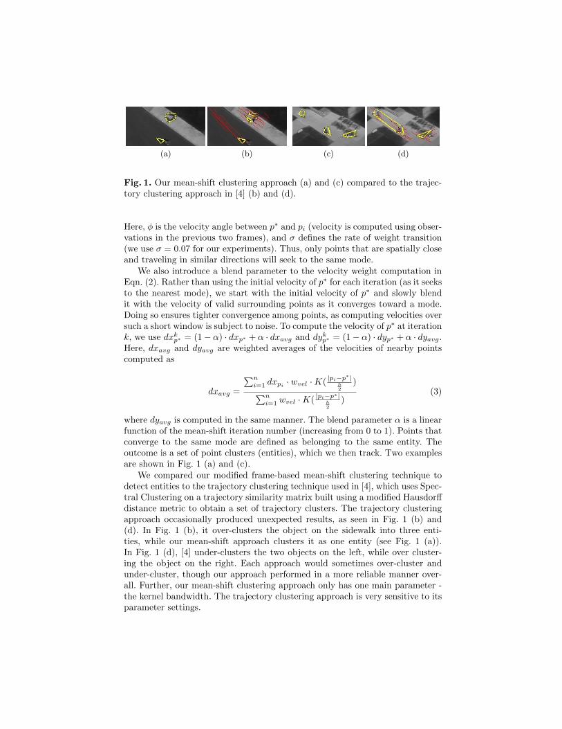
Fig. 1. Our mean-shift clustering approach (a) and (c) compared to the trajec-tory clustering approach in [4] (b) and (d).

Here, φ is the velocity angle between p∗ and pi (velocity is computed using obser-vations in the previous two frames), and σ defines the rate of weight transition(we use σ = 0.07 for our experiments). Thus, only points that are spatially closeand traveling in similar directions will seek to the same mode.

We also introduce a blend parameter to the velocity weight computation inEqn. (2). Rather than using the initial velocity of p∗ for each iteration (as it seeksto the nearest mode), we start with the initial velocity of p∗ and slowly blendit with the velocity of valid surrounding points as it converges toward a mode.Doing so ensures tighter convergence among points, as computing velocities oversuch a short window is subject to noise. To compute the velocity of p∗ at iterationk, we use dxkp∗ = (1− α) · dxp∗ + α · dxavg and dykp∗ = (1− α) · dyp∗ + α · dyavg.Here, dxavg and dyavg are weighted averages of the velocities of nearby pointscomputed as

dxavg =

∑ni=1 dxpi · wvel ·K( |pi−p

∗|h2

)∑ni=1 wvel ·K( |pi−p

∗|h2

)(3)

where dyavg is computed in the same manner. The blend parameter α is a linearfunction of the mean-shift iteration number (increasing from 0 to 1). Points thatconverge to the same mode are defined as belonging to the same entity. Theoutcome is a set of point clusters (entities), which we then track. Two examplesare shown in Fig. 1 (a) and (c).

We compared our modified frame-based mean-shift clustering technique todetect entities to the trajectory clustering technique used in [4], which uses Spec-tral Clustering on a trajectory similarity matrix built using a modified Hausdorffdistance metric to obtain a set of trajectory clusters. The trajectory clusteringapproach occasionally produced unexpected results, as seen in Fig. 1 (b) and(d). In Fig. 1 (b), it over-clusters the object on the sidewalk into three enti-ties, while our mean-shift approach clusters it as one entity (see Fig. 1 (a)).In Fig. 1 (d), [4] under-clusters the two objects on the left, while over cluster-ing the object on the right. Each approach would sometimes over-cluster andunder-cluster, though our approach performed in a more reliable manner over-all. Further, our mean-shift clustering approach only has one main parameter -the kernel bandwidth. The trajectory clustering approach is very sensitive to itsparameter settings.

3.2 Entity Tracking

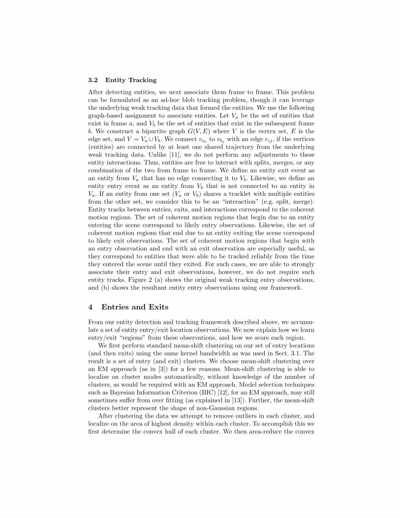
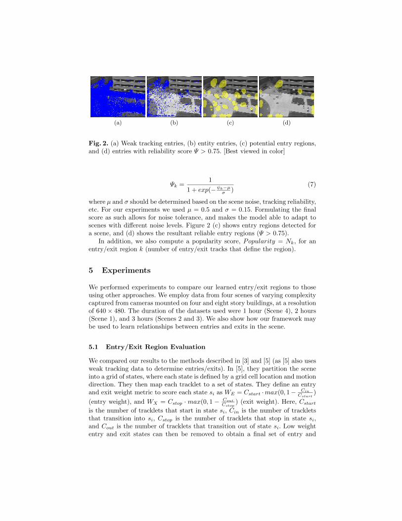
After detecting entities, we next associate them frame to frame. This problemcan be formulated as an ad-hoc blob tracking problem, though it can leveragethe underlying weak tracking data that formed the entities. We use the followinggraph-based assignment to associate entities. Let Va be the set of entities thatexist in frame a, and Vb be the set of entities that exist in the subsequent frameb. We construct a bipartite graph G(V,E) where V is the vertex set, E is theedge set, and V = Va∪Vb. We connect vai to vbj with an edge eij , if the vertices(entities) are connected by at least one shared trajectory from the underlyingweak tracking data. Unlike [11], we do not perform any adjustments to theseentity interactions. Thus, entities are free to interact with splits, merges, or anycombination of the two from frame to frame. We define an entity exit event asan entity from Va that has no edge connecting it to Vb. Likewise, we define anentity entry event as an entity from Vb that is not connected to an entity inVa. If an entity from one set (Va or Vb) shares a tracklet with multiple entitiesfrom the other set, we consider this to be an “interaction” (e.g. split, merge).Entity tracks between entries, exits, and interactions correspond to the coherentmotion regions. The set of coherent motion regions that begin due to an entityentering the scene correspond to likely entry observations. Likewise, the set ofcoherent motion regions that end due to an entity exiting the scene correspondto likely exit observations. The set of coherent motion regions that begin withan entry observation and end with an exit observation are especially useful, asthey correspond to entities that were able to be tracked reliably from the timethey entered the scene until they exited. For such cases, we are able to stronglyassociate their entry and exit observations, however, we do not require suchentity tracks. Figure 2 (a) shows the original weak tracking entry observations,and (b) shows the resultant entity entry observations using our framework.

4 Entries and Exits

From our entity detection and tracking framework described above, we accumu-late a set of entity entry/exit location observations. We now explain how we learnentry/exit “regions” from these observations, and how we score each region.

We first perform standard mean-shift clustering on our set of entry locations(and then exits) using the same kernel bandwidth as was used in Sect. 3.1. Theresult is a set of entry (and exit) clusters. We choose mean-shift clustering overan EM approach (as in [3]) for a few reasons. Mean-shift clustering is able tolocalize on cluster modes automatically, without knowledge of the number ofclusters, as would be required with an EM approach. Model selection techniquessuch as Bayesian Information Criterion (BIC) [12], for an EM approach, may stillsometimes suffer from over fitting (as explained in [13]). Further, the mean-shiftclusters better represent the shape of non-Gaussian regions.

After clustering the data we attempt to remove outliers in each cluster, andlocalize on the area of highest density within each cluster. To accomplish this wefirst determine the convex hull of each cluster. We then area-reduce the convex

hull by removing unreliable observations. We compute a density score for thepoints in each cluster via kernel density estimation [14] using only the points inthe cluster. We then remove points one at a time in ascending order of densityscore, and compute the change in area of the new convex hull after each point isremoved (the removal of outlier points will cause a large reduction of convex hullarea). Thus, we have a distribution of convex hull area changes (from remov-ing each point). We compute the variance of this distribution (assuming a zeromean), and select observations greater than σ = 1.5 standard deviations away.Of the cluster points that produced these outlier convex hull area changes, wechoose the point with the highest density score, and discard all cluster pointswith lower density scores. Thus, we have a new set of points which better repre-sent the true mass of the cluster. To generalize the shape of this new region, wecompute a kernel density surface using the new set of remaining points, deter-mine the point who is lowest on the density surface, and slice the surface at thatdensity value. The perimeter of the slice outlines the final entry or exit region.Thus, unlike [3], our entry and exit clusters reflect the true spatial density anddistribution of their underlying observations (which may not be Gaussian).

4.1 Entry/Exit Zone Reliability

We now describe how we validate our entry and exit regions to distinguish reliableentries and exits from those that are the result of noise or partial scene occlusions.In [3], they compute an entry/exit region density and then label regions withdensity below an arbitrary threshold as noise. Such an approach will not workwell if scene traffic is imbalanced, as entries/exits with low popularity (and thuslow density), may be regarded as noise. Also, if a scene is very noisy, this methodmay also classify noise as being a good entry/exit region. We define a good entryregion as one with entity tracks emanating out of it, and a good exit region asone with entity tracks flowing into it. Entry regions whose entry-only tracks (orexit regions whose exit-only tracks) exhibit bidirectional activity are unreliableregions, and may be the result of areas with a high rate of tracking failure,partial scene occlusions, or scene noise (trees or other such movement that thetracker may pick up). Further, for entry regions, other tracks in the scene shouldnot intersect the region in the same emanating direction that defines the region(i.e., the entry region should not be a “through” state). Such a scenario wouldindicate that another entry region exists behind the current one. The same ideaholds for exit regions. Thus, we attempt to capture both the consistency of theentry/exit entity tracks that define each region, as well as the consistency of theinteraction between other entity tracks and each entry/exit region.

Using the entry/exit entity tracks that define each region, we learn the distri-bution of directions that these tracks leave (for entries), and enter (for exits), theregion by quantizing the angle that each track intersects the region into one of bbins (we use b = 8 in our experiments). This histogram is normalized to providea probabilistic measure for the directions that entry/exit tracks leave/enter eachregion. From this distribution r, we compute a directional consistency functionr̂, which accounts for any symmetry of the entity track distribution for each

entry and exit region in the following manner. For a bin i with probability r(θi),every other bin probability r(θj) is subtracted from r(θi), in a weighted mannersuch that bin angles that are directly opposite of i receive high weight (as theycorrespond to bi-directional behavior), and bin angles close to i receive lowerweight. For a region k,

r̂k(θi) =max

[0,∑bj=1 wij · (rk(θi)− rk(θj))

]∑bj=1 wij · rk(θi)

· rk(θi) (4)

where wij is an angle similarity weight that give more emphasis to angles corre-sponding to bidirectional behavior with respect to θi, and is computed as

wij =

{exp(1 + cos(|θi − θj |)) if cos(|θi − θj |) < 0

0 otherwise(5)

Thus, θj is ignored if it is within 90 degrees of θi, and most heavily weighted

when it is exactly opposite of θi. For a region k,∑bi=1 r̂k(θi) is 0 when the

tracks leaving an entry (or entering an exit) are completely symmetric (and thus

strongly bi-directional), reflecting that the region is unreliable, and∑bi=1 r̂k(θi)

is 1 when a region is completely non-symmetric, and thus reliable.In addition to this directional consistency measure, we also need to capture

the way in which other tracks interact with each entry or exit region. We com-bine the previous directional consistency measure (Eqn. (4)) with an interactioncomponent to compute a total reliability score, ψ, for each region k

ψk =

(b∑i=1

r̂k(θi)

)·

(1−min

[1,

∑bi=1 r̂k(θi) ·Mk(θi)∑bi=1 r̂k(θi) ·Nk(θi)

])(6)

Here, Nk is the number of entity tracks that define an entry/exit region k,and Nk(θi) is the number of entity tracks that leave an entry (or enter an exit)region k at angle i. Similarly, Mk is the number of other entity tracks in thescene that intersect an entry/exit region, and Mk(θi) is the number of thoseentity tracks that intersect and entry/exit region k at angle i. As describedearlier, for a reliable region these tracks should not intersect an entry region inthe same direction as the entry tracks that leave it (or intersect an exit region in

the same direction as its tracks exit). The first term∑bi=1 r̂k(θi) is the directional

consistency term for the entry/exit region and acts as a prior (Eqn. (4)). Thisscore will dominate the total score if Mk = 0 (no tracks intersect the region k).If Mk > 0, and the intersecting tracks support the region as being reliable, then∑bi=1 r̂k(θi)·Mk(θi) ≈ 0. If however there are tracks that intersect the region and

contribute evidence that the region may be unreliable (due to tracking failures,

the region being partially occluded, etc.),∑bi=1 r̂k(θi)·Mk(θi)∑bi=1 r̂k(θi)·Nk(θi)

will approach 1 as

the number of discrediting intersecting tracks approaches Nk, and grow largeif the number of tracks > Nk, penalizing the region score. If Nk is 0, then wedefine the region as unreliable. Lastly, we compute a final region score as

(a) (b) (c) (d)

Fig. 2. (a) Weak tracking entries, (b) entity entries, (c) potential entry regions,and (d) entries with reliability score Ψ > 0.75. [Best viewed in color]

Ψk =1

1 + exp(−ψk−µσ )(7)

where µ and σ should be determined based on the scene noise, tracking reliability,etc. For our experiments we used µ = 0.5 and σ = 0.15. Formulating the finalscore as such allows for noise tolerance, and makes the model able to adapt toscenes with different noise levels. Figure 2 (c) shows entry regions detected fora scene, and (d) shows the resultant reliable entry regions (Ψ > 0.75).

In addition, we also compute a popularity score, Popularity = Nk, for anentry/exit region k (number of entry/exit tracks that define the region).

5 Experiments

We performed experiments to compare our learned entry/exit regions to thoseusing other approaches. We employ data from four scenes of varying complexitycaptured from cameras mounted on four and eight story buildings, at a resolutionof 640× 480. The duration of the datasets used were 1 hour (Scene 4), 2 hours(Scene 1), and 3 hours (Scenes 2 and 3). We also show how our framework maybe used to learn relationships between entries and exits in the scene.

5.1 Entry/Exit Region Evaluation

We compared our results to the methods described in [3] and [5] (as [5] also usesweak tracking data to determine entries/exits). In [5], they partition the sceneinto a grid of states, where each state is defined by a grid cell location and motiondirection. They then map each tracklet to a set of states. They define an entryand exit weight metric to score each state si as WE = Cstart ·max(0, 1− Cin

Cstart)

(entry weight), and WX = Cstop ·max(0, 1 − CoutCstop

) (exit weight). Here, Cstartis the number of tracklets that start in state si, Cin is the number of trackletsthat transition into si, Cstop is the number of tracklets that stop in state si,and Cout is the number of tracklets that transition out of state si. Low weightentry and exit states can then be removed to obtain a final set of entry and

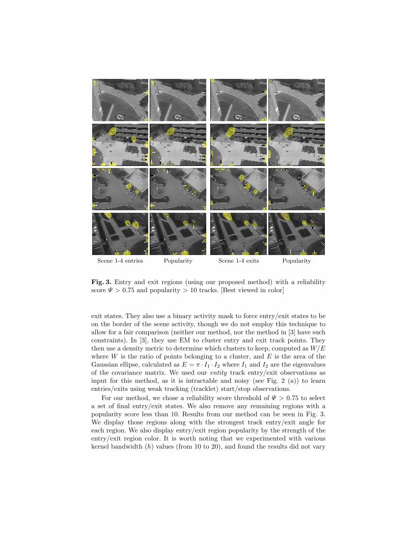
Scene 1-4 entries Popularity Scene 1-4 exits Popularity

Fig. 3. Entry and exit regions (using our proposed method) with a reliabilityscore Ψ > 0.75 and popularity > 10 tracks. [Best viewed in color]

exit states. They also use a binary activity mask to force entry/exit states to beon the border of the scene activity, though we do not employ this technique toallow for a fair comparison (neither our method, nor the method in [3] have suchconstraints). In [3], they use EM to cluster entry and exit track points. Theythen use a density metric to determine which clusters to keep, computed as W/Ewhere W is the ratio of points belonging to a cluster, and E is the area of theGaussian ellipse, calculated as E = π · I1 · I2 where I1 and I2 are the eigenvaluesof the covariance matrix. We used our entity track entry/exit observations asinput for this method, as it is intractable and noisy (see Fig. 2 (a)) to learnentries/exits using weak tracking (tracklet) start/stop observations.

For our method, we chose a reliability score threshold of Ψ > 0.75 to selecta set of final entry/exit states. We also remove any remaining regions with apopularity score less than 10. Results from our method can be seen in Fig. 3.We display those regions along with the strongest track entry/exit angle foreach region. We also display entry/exit region popularity by the strength of theentry/exit region color. It is worth noting that we experimented with variouskernel bandwidth (h) values (from 10 to 20), and found the results did not vary

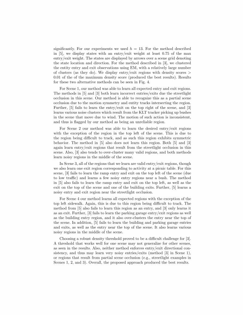
significantly. For our experiments we used h = 13. For the method describedin [5], we display states with an entry/exit weight at least 0.75 of the maxentry/exit weight. The states are displayed by arrows over a scene grid denotingthe state location and direction. For the method described in [3], we clusteredthe entity entry and exit observations using EM, with a relatively large numberof clusters (as they do). We display entry/exit regions with density scores >0.01 of the of the maximum density score (produced the best results). Resultsfor these two alternative methods can be seen in Fig. 4.

For Scene 1, our method was able to learn all expected entry and exit regions.The methods in [5] and [3] both learn incorrect entries/exits due the streetlightocclusion in this scene. Our method is able to recognize this as a partial sceneocclusion due to the motion symmetry and entity tracks intersecting the region.Further, [5] fails to learn the entry/exit on the top right of the scene, and [3]learns various noise clusters which result from the KLT tracker picking up bushesin the scene that move due to wind. The motion of such action is inconsistent,and thus is flagged by our method as being an unreliable region.

For Scene 2 our method was able to learn the desired entry/exit regionswith the exception of the region in the top left of the scene. This is due tothe region being difficult to track, and as such this region exhibits symmetricbehavior. The method in [5] also does not learn this region. Both [5] and [3]again learn entry/exit regions that result from the streetlight occlusion in thisscene. Also, [3] also tends to over-cluster many valid regions, and both methodslearn noisy regions in the middle of the scene.

In Scene 3, all of the regions that we learn are valid entry/exit regions, thoughwe also learn one exit region corresponding to activity at a picnic table. For thisscene, [3] fails to learn the ramp entry and exit on the top left of the scene (dueto low traffic) and learns a few noisy entry regions near a bush. The methodin [5] also fails to learn the ramp entry and exit on the top left, as well as theexit on the top of the scene and one of the building exits. Further, [5] learns anoisy entry and exit region near the streetlight occlusion.

For Scene 4 our method learns all expected regions with the exception of thetop left sidewalk. Again, this is due to this region being difficult to track. Themethod from [5] also fails to learn this region as an entry, and [3] only learns itas an exit. Further, [3] fails to learn the parking garage entry/exit regions as wellas the building entry region, and it also over-clusters the entry near the top ofthe scene. In addition, [5] fails to learn the building and parking garage entriesand exits, as well as the entry near the top of the scene. It also learns variousnoisy regions in the middle of the scene.

Choosing a robust density threshold proved to be a difficult challenge for [3].A threshold that works well for one scene may not generalize for other scenes,as seen in the results. Also, neither method enforces entry/exit directional con-sistency, and thus may learn very noisy entries/exits (method [3] in Scene 1),or regions that result from partial scene occlusion (e.g., streetlight examples inScenes 1, 2, and 3). Overall, the proposed approach produced the best results.

Entries from [3] Exits from [3] Entry states from [5] Exit states from [5]

Fig. 4. Entry and exit regions using the method in [3] (cols 1 and 2). Entry andexit states using the method in [5] (cols 3 and 4). [Best viewed in color]

5.2 Semantic scene actions

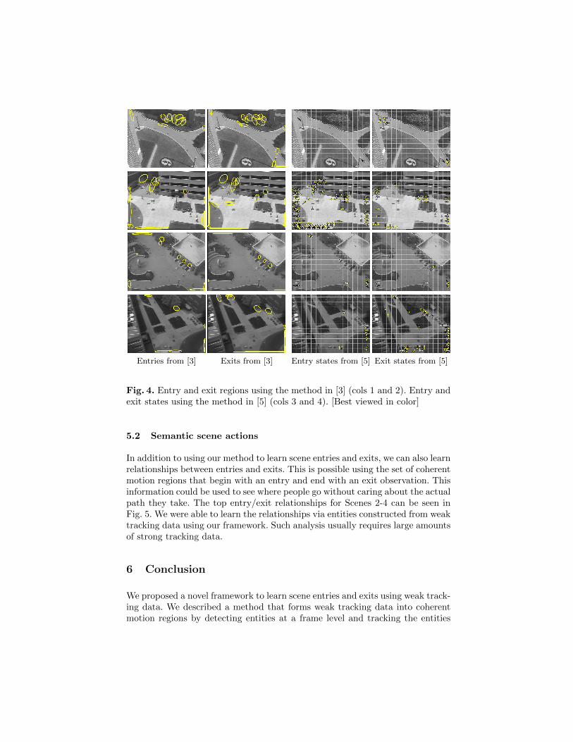
In addition to using our method to learn scene entries and exits, we can also learnrelationships between entries and exits. This is possible using the set of coherentmotion regions that begin with an entry and end with an exit observation. Thisinformation could be used to see where people go without caring about the actualpath they take. The top entry/exit relationships for Scenes 2-4 can be seen inFig. 5. We were able to learn the relationships via entities constructed from weaktracking data using our framework. Such analysis usually requires large amountsof strong tracking data.

6 Conclusion

We proposed a novel framework to learn scene entries and exits using weak track-ing data. We described a method that forms weak tracking data into coherentmotion regions by detecting entities at a frame level and tracking the entities

Scene 2 Scene 3 Scene 4

Fig. 5. Strongest activities from various scenes displayed as arrows from entryregions to exit regions. [Best viewed in color]

through time, resulting in a set of reliable spatio-temporal paths. We also intro-duced a novel scoring metric that uses the activity in the scene to reason aboutthe reliability of each entry/exit region. Results from multiple scenes showed thatour proposed method was able to learn a more reliable set of entry/exit regionsas compared to existing approaches. This research was supported in part by theUS AFRL HE Directorate (WPAFB) under contract No. FA8650-07-D-1220.

References

1. Stauffer, C.: Estimating tracking sources and sinks. In: In Proc. Second IEEEEvent Mining Workshop. (2003)

2. Shi, J., Tomasi, C.: Good features to track. In: CVPR. (1994)3. Makris, D., Ellis, T.: Automatic learning of an activity-based semantic scene model.

In: AVSS. (2003)4. Wang, X., Tieu, K., Grimson, E.: Learning semantic scene models by trajectory

analysis. In: ECCV. (2006)5. Streib, K., Davis, J.: Extracting pathlets from weak tracking data. In: AVSS.

(2010)6. Rabaud, V., Belongie, S.: Counting crowded moving objects. In: CVPR. (2006)7. Browstow, G., Cipolla, R.: Unsupervised Bayesian detection of independent motion

in crowds. In: CVPR. (2006)8. Cheriyadat, A., Bhaduri, B., Radke, R.: Detecting multiple moving objects in

crowded environments with coherent motion regions. In: POCV. (2008)9. Cheriyadat, A., Radke, R.: Automatically determining dominant motions in

crowded scenes by clustering partial feature trajectories. In: Proc. Int. Conf. onDistributed Smart Cameras. (2007)

10. Cheng, Y.: Mean shift, mode seeking, and clustering. PAMI 17 (1995)11. Masoud, O., Papanikolopoulos, N.: A novel method for tracking and counting

pedestrians in real-time using a single camera. IEEE Trans. on Vehicular Tech. 50(2001)

12. Schwarz, G.: Estimating the dimension of a model. Ann. of Statist. 6 (1978)13. Cruz-Ramirez, N., et al.: How good are the Bayesian information criterion and

the minimum description length principle for model selection? A Bayesian networkanalysis. In: Proc. 5th Mexican Int. Conf. on Artificial Intelligence. (2006)

14. Parzen, E.: On estimation of a probability density function and mode. Ann. Math.Statist. 33 (1962)