Learning a Lot from Only a Little: GeneticProgramming for Panel Segmentation on Sparse

Sensory Evaluation Data

Katya Vladislavleva1, Kalyan Veeramachaneni2, Una-May O’Reilly2,Matt Burland3, and Jason Parcon3

1 University of Antwerp, Belgium, katya@vanillamodeling.com2 Massachusetts Institute of Technology, USA, kalyan,unamay@csail.mit.edu3 Givaudan Flavors Corp., USA, matt.burland,jason.parcon@givaudan.com

Abstract. We describe a data mining framework that derives panelistinformation from sparse flavour survey data. One component of theframework executes genetic programming ensemble based symbolic re-gression. Its evolved models for each panelist provide a second componentwith all plausible and uncorrelated explanations of how a panelist ratesflavours. The second component bootstraps the data using an ensembleselected from the evolved models, forms a probability density functionfor each panelist and clusters the panelists into segments that are easyto please, neutral, and hard to please.

Key words: symbolic regression, panel segmentation, survey data, en-semble modeling, hedonic, sensory evaluation

1 Introduction

Givaudan Flavours, a leading fragrance and flavour corporation, is currently try-ing to integrate evolutionary computation techniques into its design of flavours.In one step of its design process, Givaudan conducts a hedonic survey whichpresents aromas of flavours to a small panel of targeted consumers and querieshow much each flavour is liked. Each panelist is asked to sniff roughly 50 flavours.

To best exploit the restricted sample size, Givaudan flavourists first reducethe ingredients they experimentally vary in the flavours to the most importantones. Then they use experimental design to define a set that statistically providesthem with the most information about responses to the entire design space.

The specificity of sensory evaluation data is such, that “the panelist to pan-elist differences are simply too great to ignore as just an inconvenience of thescientific quest,” [1], because “taste and smell, the chemical senses, are primeexamples of inter-panelist differences, especially in terms of the hedonic tone (lik-ing/disliking),” [1]. Givaudan employs reliable statistical techniques that regressa single model from the survey data. This model describes how much the panel,as an aggregate, likes any flavour in the space. But since the differences in theliking preferences of the panelists are significant, Givaudan is also using several

proprietary methods to deal with the variation in the panel and is interested inalternative techniques.

A goal of our interaction with Givaudan is to generate innovative informa-tion about the different panelists and their liking-based responses by developingtechniques that will eventually help Givaudan design even better flavours. Herewe describe how Genetic Programming (GP) can be used to model sensory eval-uation data without suppressing the variation that comes from humans havingdifferent flavour preferences. We also describe how GP enables a knowledge min-ing framework, see Figure 1, that meaningfully segments (i.e. clusters) the panel.With an exemplar Givaudan dataset, we identify the panelists who are ”easy toplease”, i.e. that frequently respond with high liking to flavours, ”hard to please”and ”neutral”. This is, in general, challenging because the survey data is sparse.In this particular dataset there are only 40 flavours in the seven-dimensionalsample set and 69 panelist responses per flavour.

Create Multiple Plausible Explanations

of the Data

Bootstrap Liking Scores

1746

1249)exp( 2

3

31

x

xx

Derive Liking Score Density Model

Cluster

0 2 4 6 8 10 120

0.05

0.1

0.15

0.2

0.25

0.3

0.35

Liking score

Pro

bab

ilit

y D

en

sit

y

Weibull Distribution of Liking Score

Ωs sY

)(LSps

HSES NS

, s

oo SL F

Panelist loop

GP Module

Fig. 1. Knowledge mining framework for sparse sensory data with a focus on panelsegmentation. Read clockwise. The top portion is repeated for each panelist

We proceed as follows: Section 2 introduces our flavour-liking data set. Sec-tion 3 discusses why GP model ensembles are well suited for this problem domainand briefly cites related work. Section 4 outlines the 5 steps of our method. Sec-tion 5 describes Steps 1 and 2, the ensemble derivation starting from ParetoGP.Section 6 presents Steps 3-5 – how the probability density functions and clustersthat ultimately answer the questions are derived from this ensemble, and ourexperimental results. Section 7 concludes and mentions future work.

2 The Givaudan Flavour Liking Data Set

In this data set, flavour space consists of seven ingredients called keys, ki. Aflavour in the flavour space is a mixture by volume of these seven ingredients

and the j th flavour is denoted by k(b)

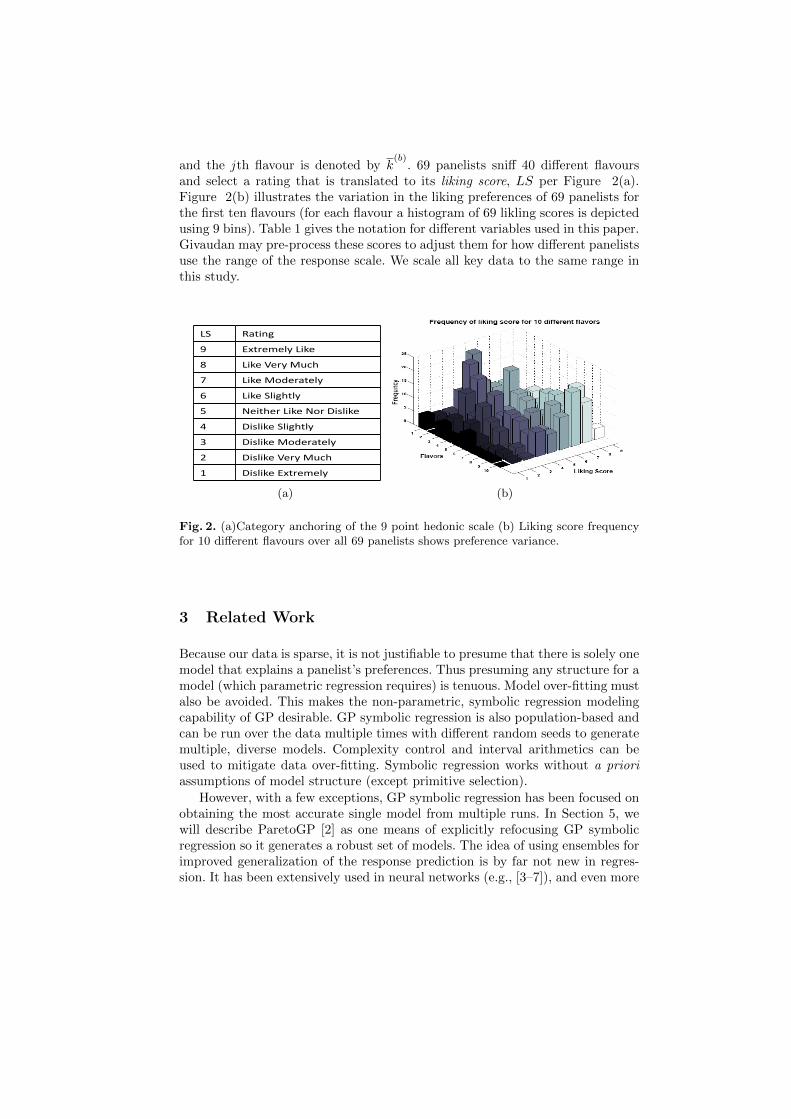
. 69 panelists sniff 40 different flavoursand select a rating that is translated to its liking score, LS per Figure 2(a).Figure 2(b) illustrates the variation in the liking preferences of 69 panelists forthe first ten flavours (for each flavour a histogram of 69 likling scores is depictedusing 9 bins). Table 1 gives the notation for different variables used in this paper.Givaudan may pre-process these scores to adjust them for how different panelistsuse the range of the response scale. We scale all key data to the same range inthis study.

LS Rating

9 Extremely Like

8 Like Very Much

7 Like Moderately

6 Like Slightly

5 Neither Like Nor Dislike

4 Dislike Slightly

3 Dislike Moderately

2 Dislike Very Much

1 Dislike Extremely

(a) (b)

Fig. 2. (a)Category anchoring of the 9 point hedonic scale (b) Liking score frequencyfor 10 different flavours over all 69 panelists shows preference variance.

3 Related Work

Because our data is sparse, it is not justifiable to presume that there is solely onemodel that explains a panelist’s preferences. Thus presuming any structure for amodel (which parametric regression requires) is tenuous. Model over-fitting mustalso be avoided. This makes the non-parametric, symbolic regression modelingcapability of GP desirable. GP symbolic regression is also population-based andcan be run over the data multiple times with different random seeds to generatemultiple, diverse models. Complexity control and interval arithmetics can beused to mitigate data over-fitting. Symbolic regression works without a prioriassumptions of model structure (except primitive selection).

However, with a few exceptions, GP symbolic regression has been focused onobtaining the most accurate single model from multiple runs. In Section 5, wewill describe ParetoGP [2] as one means of explicitly refocusing GP symbolicregression so it generates a robust set of models. The idea of using ensembles forimproved generalization of the response prediction is by far not new in regres-sion. It has been extensively used in neural networks (e.g., [3–7]), and even more

Table 1. Problem Specific Variable Description

Variable Notation Details

flavour Space F The design space of ingredient mixtures

Keys ki i ∈ 1...7flavour k A mixture of 7 keys, k = k1, ...k7

A specific flavour k(b)

A specific flavour denoted by superscript b

Panelist sn n ∈ 1..69Set of Panelists S S = s1, s2, ....s69

Observed flavours Fo Fo = k(1)....k(40)Bootstrapped flavours FB FB = k(1)......k(10,000)

Likability Function fs(k(j)

) = LS Relationship between a k(b)

and LS

lsd p(LS|s) Liking score density function for a panelist s

Cumulative density Px(LS ≥ x|s) Probability of Liking score ≥ xPanelist Cluster Sc A subset of S, c ∈ E,N,H

Model m Model m for Panelist s

Prediction ys,b,m Model m’s prediction for a k(b)

Model Ensemble Ωs All models in the ensemble

Prediction Set Ys,b

Ys,b

= ∀m ∈ Ωs ys,b,mSet of Liking Scores s Y

sY

s= ∀b ∈ FB Y

s,b

extensively in boosting and machine learning in general (albeit, mostly for classi-fication). See [8–14] for examples. [7] presented the idea of using disagreement ofensemble models for quantifying the ambiguity of ensemble prediction for neuralnetworks, but the approach has not been adapted to symbolic regression.

4 Panel Data Mining Steps

Our GP ensemble-based ”knowledge mining” method has five steps:

1. Generate a diverse model set for each panelist from the sparse samples.2. Thoughtfully select an ensemble of models meeting accuracy and complex-

ity limits to admit generalization and avoid overfitting and a correlationthreshold to avoid redundancy.

3. Use all models of the ensemble to generate multiple predictions for manyunseen inputs.

4. With minor trimming of the extremes and attention to the discrete natureof liking scores, fit the predictions to a Weibull distribution.

5. Cluster based on the Weibull distribution’s probability mass.

It is significant to note that these steps respect the importance of avoidingpremature elimination of any plausible information because the data is sparse.The ensemble provides all valid values of the random variable when it is presented

with new inputs. This extracts maximum possible information about the randomvariable, which supports more robust density estimation.

We proceed in Section 5 to detail how we assemble a symbolic regressionensemble, i.e. Steps 1 and 2. In Section 6, we detail Steps 3 through 5.

5 A Symbolic Regression Ensemble

ParetoGP Select Models

, s

oo SL F

)exp( 2

3

31

x

xx

)exp( 2

3

31

x

xxΩs

Diverse and RichModel Ensemble

Fig. 3. Ensemble based symbolic regression

Traditionally symbolic regression has been designed for generating a singlemodel. Researchers have focused on evolving the model that best approximatesthe data and identifies hidden relationships between variables. They have de-veloped multiple competent approaches to over-fitting. There are a number ofdemonstrably effective procedures for selecting the final model from the GPsystem. Machine learning techniques such as cross validation and bagging havebeen integrated. Multiple ways of controlling expression complexity are effective.See [15] for a thorough justification of the above assessment.

Modelers who must provide all and any explanations for the data are not wellserved by this emphasis upon a single model. Any algorithm variation of symbolicregression, even one that proceeds with attention to avoiding over-fitting, is asfragile as a parametric model with respect to the accuracy of its predictions andthe confidence it places in those predictions if it outputs one model. The risksare maximal when the best-of-the-run model is selected from the GP systemas the solution. Our opinion is supported by the evidence in [16] which showsthat symbolic regression performed with complexity control, interval arithmetic,and linear scaling still produces over-fitted best-error-of-the-run models thatfrequently have extrapolation pathologies.

Symbolic regression can handle dependent and correlated variables and au-tomatically perform feature selection. It is capable of producing hundreds of

candidate models that explain sparse data via diverse mathematical structureand parameters. But the combined information of these multiple models hasbeen conventionally ignored. In our framework, we exploit rather than ignorethem. During a typical run, GP symbolic regression explores numerous models.We capture the combined explanatory content of fitness-selected models, andpool as many explanations as we can from whatever little data we have.

An explicit implementation of this strategy, such as ParetoGP, must embedoperators and evaluation methods into the GP algorithm to specifically aggre-gate a rich model set after combining multiple runs. The set will support deriv-ing an ensemble of high-quality but diverse models. Within an ensemble, eachmodel must approximate all training data samples well – high quality. As an en-semble, the models must collectively diverge in their predictions on unobserveddata samples –diverse. If a GP symbolic regression system can yield a sufficientquantity of “strong learners” as its solution set, all of them can and should beused to determine both a prediction, and the ensemble disagreement (lack ofconfidence) at any arbitrary point of the original variable space. In contrast toboosting methods that are intended to improve the prediction accuracy througha combination of weak learners into an ensemble, this ensemble derivation pro-cess has the intent of improving prediction robustness and estimating reliabilityof predictions.

5.1 Model set Generation

All experiments of this paper use the ParetoGP algorithm which has been specif-ically designed to meet the goals of ensemble modeling. Any other GP systemdesigned for the same goals would suffice. ParetoGP consists of the tree-based GPwith multi-objective model selection optimizing the trade-off between a model’straining error and expressional complexity; an elite-preservation strategy (alsoknown as archiving), interval arithmetic, linear scaling and Pareto tournamentsfor selecting crossover pairs. In each iteration of the algorithm, it tries to closelyapproximate the (true) Pareto curve trade-offs between accuracy and complex-ity. It supports a practical rule-of-thumb: “use as many independent GP runs asthe computational budget allows”, by providing an interface where only the bud-get has to be stated to control the length of a run. It also has explicit diversitypreservation mechanisms and efficiently supports a sufficiently large populationsize. The training error used in experiments is 1− R2, where R is a correlationcoefficient of the scaled model prediction and the scaled observed response. Theexpressional complexity of models is defined as the total sum of nodes in allsubtrees of the tree-based model genome. The following primitives are used forgp trees of maximal arity of four: +,−, ∗, /, inverse, square, exp, ln. Variablesx1 − x7 corresponding to seven keys and constants from the range [−5, 5] areused as terminals. ParetoGP is executed for 6 independent runs per panelist databefore the models from runs are aggregated and combined. The population sizeequals 500, the archive size is 100. Crossover rate is 0.9, and sub-tree mutationrate is 0.1. ParetoGP collects all models on the Pareto front of each run andfor information purposes identifies a “super” Pareto front from among them. All

models move forward to ensemble selection. We now have to make a decisionabout which models will be used to form an ensemble.

5.2 Ensemble Model Selection

In [17], the authors describe an approach to selecting the models which form anensemble: collect models that differ according to complexity, prediction accuracyand specific predictions. Complexity can be measured by examining some quan-tity associated with the GP expression tree or by considering how non-linear theexpression is. Accuracy is the conventional error measure between actual andpredicted observations. Specific predictions are considered to assess correlationsand eliminate correlated models. Generally, each ensemble combines:

– A “box” of non-dominated and dominated models in the dual objective spaceof model prediction error and model complexity.

– A set of models with uncorrelated prediction errors on a designated test setof inputs. Here a model is selected based on a metric which expresses howits error vector correlates with other models’ error vector. The correlationmust not exceed a value of ρ. The input samples used to compute predictionerrors can belong to the training set, test set (if available), or be arbitrarilysampled from the observed region.

The actual ρ and box thresholds for the ensemble selection depend on theproblem domain’s goals. For this knowledge mining framework, where the nextstep is to model a probability density function of a liking score, all plausibleexplanations of the data are desired to acknowledge the variation we expect to seein human preferences. The box thresholds are accuracy = 0.5 and expressionalcomplexity < 400. This generates models with sufficient generality (since weallowed accuracy as low as 0.5) and restricts any models with unreasonablyhigh complexity with no obvious improvement in accuracy. We chose a value ofρ = 0.92 to weed out correlated models. A set of models selected after applyingthe criteria above is called the ensemble, Ωs.

6 Modeling a Panelist’s Propensity to Like

With methods that support refocusing GP based symbolic regression to derive arich and diverse set of models and the methods [17] that select an ensemble, ourGP system becomes a competent cornerstone in our knowledge mining frame-work. The framework can next use the ensemble, Ωs designed for a panelist s toanswer the question: ”How likely is a panelist to answer with a liking score/ratinghigher than X?”. The answer to this question allows us to categorize panelistsas: (1) Easy to Please, (2) Hard to Please, (3) Neutral. We accomplish this bymodeling the probability density function given by p(LS|s) for a panelist s. Todescribe our methodology, we rely upon the notations in Table 1.

Density estimation poses a critical challenge in machine learning, especiallywith sparse data. Even if we assume that we have finite support for the density

function and it is discrete, i.e. LS = 1, 2, ...8, 9, we need sample sizes of theorder of ”supra-polynomial” in the cardinality of support [18]. In addition, ifthe decision variables are inter-dependent, as they are here, estimating a condi-tional distribution increases the computational complexity. Most of the researchin density estimation has focused on identifying non-parametric methods to esti-mate distribution of the data. Research on estimation of density from very smallsample sizes is limited [18,19].

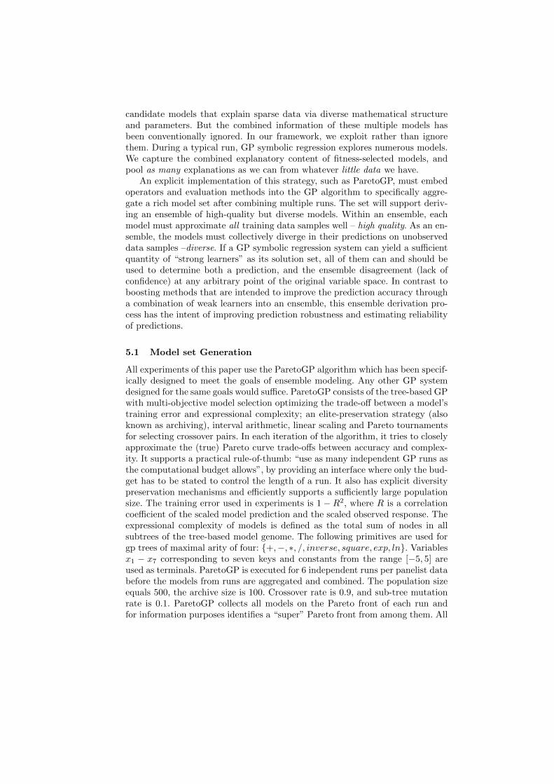
Figure 4 presents the steps taken to form this liking score probability densitymodel. We first generate 10,000 untested flavours We use the model ensemble

Ωs, which gives us a set of predictions Ys,b

.For each untested flavour we get aset of predictions (not just one), which plausibly represents all possible likingscores the panelist would give. We use these to construct the lsd, liking scoredensity function, for an individual panelist.

Boot strap DataSee Algorithm 1

Parametric Estimation to

Weibull

1746

1249

)exp( 2

3

31

x

xx

0 2 4 6 8 10 120

0.05

0.1

0.15

0.2

0.25

0.3

0.35

Liking score

Pro

bab

ilit

y D

en

sit

y

Weibull Distribution of Liking Score

Ωs

sYbFs sr,

Fig. 4. Bootstrapping the Data and Deriving the Liking Score Probability DensityModel

6.1 Deriving Predictions by Bootstrapping the Data

To generate the bootstrapped data of liking scores for the FB = k(1)......k(10,000)we follow the steps described in Algorithm 1.

Algorithm 1 Bootstrapping the LS data for Panelist s

Generate 10,000 flavours randomly, i.e., Fb = k1....k10,000 (we use a fixed uniformlattice in the experiments, same for all panelists)

for (kb ∈ Fb ∀b) do

(i)Collect all the predictions from Model Ensemble, Ωs: Ys,b

(ii) Sort the vector Ys,b

(iii) Remove the bottom and top 10% of Ys,b

and call this vector Rs,j

(iv) Append Rs,j

to Ys

end forFit the Y

sto a Weibull distribution. See Section 6.2

6.2 Parametric Estimation of the Liking Score Density Function

We use a parametric Weibull distribution to estimate p(LS|s). The two parame-ters for the Weibull distribution, λ and r are called scale and shape respectively.A Weibull distribution is an adaptive distribution that can be made equivalent toan Exponential, Gaussian or Rayleigh distributions as its shape and scale param-eters are varied. For our problem this is a helpful capability as a panelist’s likingscore follows any one of the three distributions. The derived Weibull distributionis:

p(LS;λ, r|s) =

rλ (LSλ )r−1e−(LSλ )r if LS ≥ 0

0 if LS < 0.(1)

In addition to steps taken in Section 6.1, we map the bootstrapped data to arange of the support of Weibull and the hedonic rating scale i.e., [1, 9]. There aresome predictions in the Y

swhich are below 1 or are above 9. We remove 80% of

these predictions as outliers. We assign a liking score of 1 for the remaining 20%of predictions that are less than ’1’ in the prediction set. We similarly assignthe liking score of ’9’ for the ones that are above 9. We use these 20% in Y

sto

capture the scores corresponding to the ”extremely dislike” and ”extremely like”condition. Each plot line of Figures 6 (b), (c) and (d) is a lsd.

6.3 Clustering Panelists by Propensity to Like

Define Decision Regions

See Algorithm 2

Evaluate CDF in each Region

Assign Cluster as the region with maximum CDF

ssr,

Fig. 5. Clustering the Panelists

Having estimated the data generated from the models for 10,000 flavours

in FB = k(1)......k(10,000) using the methods described in Section 6.2, we canclassify the panelists into three different categories (see Figure 5). We divide theliking score range [1..9] into three regions as shown in Figure 6. The panelistsare then classified by identifying the region in which the majority (more than50%) of their probability mass lies (see Algorithm 2). This is accomplished byevaluating the cumulative distribution in each of these regions using:

P(l1,l2](LS;λ, r|s) = e−( l1λ )r

− e−( l2λ )r

. (2)

Algorithm 2 Clustering the Panelists

for ∀s ∈ S do1. Calculate Pl1,l2 using estimated (λs, rs) for (l1, l2] → (1, 3.5], (3.5, 6.5] and(6.5, 9.5]2. Assign the panelist s, to the cluster corresponding to the region where he/shehas maximum cumulative densitys← s+ 1

end for

6.4 Results on All Panelists

We applied our methodology to the dataset of 66 panelists who can be individ-ually modeled with adequate accuracy. The first cluster is the ”hard to please”panelists. We have 23 panelists in this cluster which is approximately 34.8% ofthe panel. These panelists have most of their liking scores concentrated between1-3.5 range. We call these ”hard-to-please” since low liking scores might implythat they are very choosy in their liking.

The second cluster is the cluster of ”neutral panelists”. These panelists rarelychoose the liking scores which are extremely like or extremely dislike. For mostof the sampled flavours they choose somewhere in between and hence the nameneutral. There are 31 panelists in this cluster which is 47% of the total panel.

The final cluster of panelists is the ”easy to please” panelists. This cluster ofpanelists reports a high liking for most of the flavours presented to them or mayreport moderate dislike of some. They rarely report ”extremely dislike”. Thereare 12 panelists in this cluster which is close to 18% of the total panel.

7 Conclusions and Future Work

This contribution described an ensemble-based symbolic regression approach forknowledge mining from a very small sample of survey measurements. It is onlya first small step towards GP-driven flavour optimization and also demonstratesthe effectiveness of GP for sparse data modeling. Our goal was to model behav-ior of panelists who rate flavours. Our methodology postpones decision makingregarding a model, a prediction, and a decision boundary until the very end. InStep 1 ParetoGP generates a rich set of models consisting of the multiple plau-sible explanations for the data from multiple run aggregation of its best models.In Step 2 these are filtered into an efficient and capable ensemble and no validexplanation is eliminated. In Step 3 all the models are consulted, and with mi-nor trimming, their predictions are fit to a probability density function. Finally,in Step 4, when macro-level behaviour has emerged and more is known aboutthe panelists, decision boundaries can be rationally imposed on this probabilityspace to allow their segmentation. Our approach allowed us to robustly identifysegments in the panel based on the liking preferences. We conjecture from ourresults that there are similar potential benefits across any sparse, repeated mea-

0 2 4 6 8 10 120

0.05

0.1

0.15

0.2

0.25

0.3

0.35

Liking score

Pro

bab

ilit

y D

en

sit

y

Weibull Distribution of Liking Score

Easy to Please

Neutral

Hard to Please

Outliers

(a)

1 2 3 4 5 6 7 8 9 10 11 120

0.1

0.2

0.3

0.4

0.5

0.6

0.7

0.8

0.9

1

8, 10,

12, 14, 15,

17, 19, 20,

23, 25, 28,

29, 32, 40,

42, 44,

53,

54, 59,

62,

64, 66, 67

Panelists:

Probability Density Function of Liking Scores of Similar Panelists

Liking Score

Pro

babi

lity

Den

sity

(b)

1 2 3 4 5 6 7 8 9 10 11 120

0.1

0.2

0.3

0.4

0.5

0.6

0.7

0.8

0.9

1

1,

2,

3,

4, 5,

6, 7,

11,

13, 18,

22,

24, 26,

30,

31, 33,

34,

35, 36,

37,

38, 41,

45,

49,

50,

51,

52,

57, 61,

63,

65

Panelists:

Probability Density Function of Liking Scores of Similar Panelists

Liking Score

Pro

babi

lity

Den

sity

(c)

1 2 3 4 5 6 7 8 9 10 11 120

0.1

0.2

0.3

0.4

0.5

0.6

0.7

0.8

0.9

1

9, 21,

27, 43, 46,

47, 48, 55,

56, 58, 68,

69

Panelists:

Probability Density Function of Liking Scores of Similar Panelists

Liking Score

Pro

babi

lity

Den

sity

(d)

Fig. 6. Liking Score Density Models: (a)Decision regions for evaluating cumulativedistribution, (b) Hard to please panelists (c) Neutral Panelists (d) Easy to PleasePanelists

sure dataset. We will focus our efforts in the future on the theory and practiceof efficient techniques for ensemble derivation in the context of GP.

Acknowledgements

We acknowledge funding support from Givaudan Flavors Corp. and thank GuidoSmits and Mark Kotancheck.

References

1. Moskowitz, H.R., Bernstein, R.: Variability in hedonics: Indications of world-widesensory and cognitive preference segmentation. Journal of Sensory Studies 15(3)(2000) 263–284

2. Smits, G., Kotanchek, M.: Pareto-front exploitation in symbolic regression. InO’Reilly, U.M., Yu, T., Riolo, R.L., Worzel, B., eds.: Genetic Programming Theoryand Practice II. Springer, Ann Arbor (2004)

3. Liu, Y., Yao, X., Higuchi, T.: Evolutionary ensembles with negative correlationlearning. IEEE Transactions on Evolutionary Computation 4(4) (2000) 380

4. Liu, Y., Yao, X.: Learning and evolution by minimization of mutual information.In: PPSN VII: Proceedings of the 7th International Conference on Parallel ProblemSolving from Nature, London, UK, Springer-Verlag (2002) 495–504

5. Hansen, L.K., Salamon, P.: Neural network ensembles. IEEE Trans. Pattern Anal.Mach. Intell. 12(10) (1990) 993–1001

6. Wolpert, D.H.: Stacked generalization. Neural Networks 5(2) (1992) 241–2597. Krogh, A., Vedelsby, J.: Neural network ensembles, cross validation, and active

learning. In Tesauro, G., Touretzky, D., Leen, T., eds.: Advances in Neural In-formation Processing Systems. Volume 7., Cambridge, MA, USA, The MIT Press(1995) 231–238

8. Paris, G., Robilliard, D., Fonlupt, C.: Applying boosting techniques to geneticprogramming. In Collet, P., Fonlupt, C., Hao, J.K., Lutton, E., Schoenauer, M.,eds.: Artificial Evolution 5th International Conference, Evolution Artificielle, EA2001. Volume 2310 of LNCS., Creusot, France, Springer Verlag (2001) 267–278

9. Iba, H.: Bagging, boosting, and bloating in genetic programming. In Banzhaf, W.,Daida, J., Eiben, A.E., Garzon, M.H., Honavar, V., Jakiela, M., Smith, R.E., eds.:Proceedings of the Genetic and Evolutionary Computation Conference. Volume 2.,Orlando, Florida, USA, Morgan Kaufmann (1999) 1053–1060

10. Schapire, R.E.: The strength of weak learnability. Machine Learning 5(2) (1990)197–227

11. Freund, Y., Seung, H.S., Shamir, E., Tishby, N.: Information, prediction, and queryby committee. In: Advances in Neural Information Processing Systems 5, [NIPSConference], San Francisco, CA, USA, Morgan Kaufmann Publishers Inc. (1993)483–490

12. Sun, P., Yao, X.: Boosting kernel models for regression. In: ICDM ’06: Proceedingsof the Sixth International Conference on Data Mining, Washington, DC, USA,IEEE Computer Society (2006) 583–591

13. Freund, Y.: Boosting a weak learning algorithm by majority. Inf. Comput. 121(2)(1995) 256–285

14. Folino, G., Pizzuti, C., Spezzano, G.: GP ensembles for large-scale data classifica-tion. IEEE Trans. Evolutionary Computation 10(5) (2006) 604–616

15. Vladislavleva, E.: Model-based Problem Solving through Symbolic Regression viaPareto Genetic Programming. PhD thesis, Tilburg University, Tilburg, the Nether-lands (2008)

16. Vladislavleva, E.J., Smits, G.F., den Hertog, D.: Order of nonlinearity as a com-plexity measure for models generated by symbolic regression via pareto geneticprogramming. IEEE Transactions on Evolutionary Computation 13(2) (2009)333–349

17. Kotanchek, M., Smits, G., Vladislavleva, E.: Trustable symoblic regression mod-els. In Riolo, R.L., Soule, T., Worzel, B., eds.: Genetic Programming Theory andPractice V. Genetic and Evolutionary Computation. Springer, Ann Arbor (2007)203–222

18. Taylor, J.S., Dolia, A.: A framework for probability density estimation. InLawrence, N., ed.: Proceedings of the Eleventh International Conference on Ar-tificial Intelligence and Statistics, Journal of Machine Learning Research (2007)468–475

19. Mukherjee, S., Vapnik, V.: Multivariate density estimation: a support vector ma-chine approach. In: In NIPS 12, Morgan Kaufmann Publishers (1999)