Embed Size (px)
Citation preview
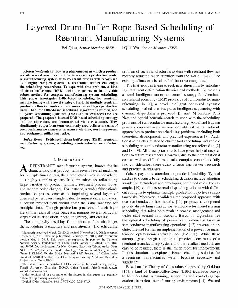
178 IEEE TRANSACTIONS ON SEMICONDUCTOR MANUFACTURING, VOL. 26, NO. 2, MAY 2013
Layered Drum-Buffer-Rope-Based Scheduling ofReentrant Manufacturing Systems
Fei Qiao, Senior Member, IEEE, and Qidi Wu, Senior Member, IEEE
Abstract—Reentrant flow is a phenomenon in which a productrevisits several machines multiple times on its production route.A manufacturing system with reentrant flow is well recognizedas a highly complex system. Its reentrance feature challengesthe scheduling researchers. To cope with this problem, a kindof drum-buffer-rope (DBR) technique proves to be a viablerobust method for complex manufacturing system scheduling.This paper investigates DBR-based scheduling for reentrantmanufacturing with a novel strategy. First, the multiple reentrantproduction flow is transferred into nonreentrant layer productionlines. Then, the DBR-based scheduling algorithm is studied, anda layered scheduling algorithm (LSA) and the extended LSA areproposed. The proposed layered DBR-based scheduling strategyand the algorithms are demonstrated via a case study. Theysignificantly outperform some commonly used policies in terms ofsuch performance measures as mean cycle time, work-in-process,and equipment utilization ratios.
Index Terms—Bottleneck, drum-buffer-rope (DBR), reentrantmanufacturing system, scheduling, semiconductor manufactur-ing.
I. Introduction
A “REENTRANT” manufacturing system, known for itscharacteristic that product items revisit several machines
for multiple times during their production lives, is consideredas a highly complex system. Its complexities are reflected bylarge varieties of product families, reentrant process flows,and random order changes. For instance, a wafer fabrication’sproduction process consists of imprinting several layers ofchemical patterns on a single wafer. To imprint different layers,a certain product item would enter the same machine formultiple times. Though production processes of each layerare similar, each of those processes requires several particularsteps such as deposition, photolithography, and etching.
The complexity resulting from reentrant flow challengesthe scheduling researchers and practitioners. The scheduling
Manuscript received March 22, 2012; revised November 24, 2012; acceptedFebruary 5, 2013. Date of publication February 25, 2013; date of currentversion May 1, 2013. This work was supported in part by the NationalNatural Science Foundation of China under Grants 61034004, 61273046,and 50905129, the Program for New Century Excellent Talents under GrantNCET-07-0622, the Science and Technology Commission of Shanghai underGrant 11ZR1440400, the Major National S&T Program of China underGrant 2011ZX03005-004-01, and the Shanghai Leading Academic DisciplineProject under Grant B004.
The authors are with the School of Electronics and Information Engineering,Tongji University, Shanghai 200093, China (e-mail: [email protected];[email protected]).
Color versions of one or more of the figures in this paper are availableonline at http://ieeexplore.ieee.org.
Digital Object Identifier 10.1109/TSM.2013.2248763
problem of such manufacturing system with reentrant flow hasrecently attracted much attention from the world [1]–[2]. Theexisting efforts can be classified into two categories.
The first group is trying to seek new algorithms by introduc-ing intelligent optimization theories and methods. [3] presentsa novel intelligent run-to-run control strategy for chemical-mechanical polishing (CMP) processes of semiconductor man-ufacturing. In [4], a novel intelligent optimized dynamicscheduling method that integrates intelligent sequencing withdynamic dispatching is proposed. [5] and [6] combine PetriNets and hybrid heuristic search to cope with the schedulingproblems of semiconductor manufacturing. Akyol and Bayhangive a comprehensive overview on artificial neural networkapproaches to production scheduling problems, including boththeoretical developments and practical experiences [7]. Addi-tional researches related to cluster tool scheduling and vehiclescheduling in semiconductor manufacturing are referred to [2]and [8]–[9]. All these prior efforts have given helpful inspira-tions to future researchers. However, due to the computationalcost as well as difficulties to take complex constraints fullyinto consideration, there exists a large gap between researchand practice in this area.
Others pay more attention to practical feasibility. Typicalstudies to obtain a better scheduling decision include adoptingsimulation technology and developing combined rules. For ex-ample, [10] combines several dispatching criteria with differ-ent strengths to optimize multiple production objectives simul-taneously. Moreover, it validates the proposed approach withtwo semiconductor fab models. [11] proposes a compoundpriority dispatching strategy for semiconductor manufacturingscheduling that takes both work-in-process management andwafer start control into account. Based on algorithms forthe optimal scheduling of preventive maintenance tasks insemiconductor manufacturing operations, [12] presents an ar-chitecture and further, an implementation of a preventive main-tenance optimization software tool (PMOST). While theseattempts give enough attention to practical constraints of areentrant manufacturing system, and the resultant methods areeasy to be realized, there is still much room for improvement.In this situation, to explore a better scheduling solution fora reentrant manufacturing system becomes necessary andsignificant.
Based on the Theory of Constraints suggested by Goldratt[13], a kind of Drum-Buffer-Rope (DBR) technique provesto be successful in planning, scheduling and controlling op-erations in various manufacturing environments [14]. Wu and
0894–6507/$31.00 c© 2013 IEEE
QIAO AND WU: LAYERED DRUM-BUFFER-ROPE BASED SCHEDULING OF REENTRANT MANUFACTURING SYSTEMS 179
Morris discuss its application in furniture manufacturing [15].The simulation results indicate considerable savings in make-span due to such a DBR strategy. [16] shows that a DBRcontrol mechanism performs well in a job shop environment.[14] investigates a number of priority dispatching rules in com-bination with DBR for recoverable manufacturing systems.
The existing researches show that DBR is applicable tolarge-scale complex system scheduling problems because itfocuses on dealing with critical constraints of those systems.Therefore, this paper will adopt a DBR mechanism to investi-gate such systems with reentrant flow. Section II gives a gen-eral layered DBR-based scheduling architecture. Section IIIdefines the concepts of main bottleneck and layer bottleneckbased on bottleneck analysis. After that, a layered schedulingalgorithm (LSA) and an extended one are proposed anddiscussed in Section IV. The application of the proposed algo-rithms is given in Section V. Section VI concludes this paper.
II. Layered DBR-Based Scheduling Architecture
The nature of reentrant flow challenges scheduling decisionmakers in the semiconductor wafer manufacturing industry.Though there are plenty of existing approaches in generalproduction scheduling already, most of them cannot be directlyemployed to deal with reentrant manufacturing scheduling.That is because of the complications arising from the system’sreentrant flow, large scale and high uncertainty. However, aDBR method has been proved to be a viable, robust methodfor complex manufacturing scheduling [14]–[16]. In this work,we intend to utilize it to find a new solution for reentrantmanufacturing scheduling problems.
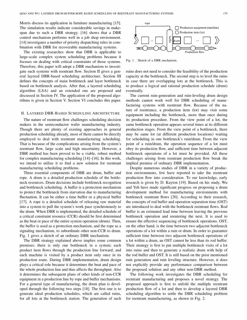
Three essential components of DBR are drum, buffer andrope. A drum is a detailed production schedule of the bottle-neck resources. Drum decisions include bottleneck recognitionand bottleneck scheduling. A buffer is a protection mechanismto protect the bottleneck from starvation due to manufacturingfluctuation. It can be either a time buffer or a physical buffer[17]. A rope is a detailed schedule of releasing raw materialinto a system to pull the system’s work pace synchronously tothe drum. When DBR is implemented, the detailed schedule ofa critical constraint resource (CCR) should be first determinedas the beat or pace of the entire system operation (drum). Then,the buffer is used as a protection mechanism, and the rope as asignaling mechanism, to subordinate other non-CCR to drum.Fig. 1 gives a sketch of an ordinary DBR mechanism.
The DBR strategy explained above implies some commonpremises: there is only one bottleneck in a system; eachproduct item flows through the production line forward; andeach machine is visited by a product item only once in itsproduction route. During DBR implementation, drum designplays a critical role because it determines the beat and pace ofthe whole production line and thus affects the throughput. Alsoit determines the subsequent plans of other kinds of non-CCRequipment in a production line by rope and buffer mechanisms.For a general type of manufacturing, the drum plan is devel-oped through the following two steps [18]. The first one is togenerate ideal production schedules, which are called ruins,for all lots at the bottleneck station. The generation of such
Fig. 1. Sketch of a DBR mechanism.
ruins does not need to consider the feasibility of the productioncapacity at the bottleneck. The second step is to level the ruinsin case there are overlapping lots at the bottleneck. This isto produce a logical and rational production schedule (drum)eventually.
The current ruin-generation and ruin-leveling drum designmethods cannot work well for DBR scheduling of manu-facturing systems with reentrant flow. Because of the na-ture of reentrance, a production item (lot) may visit someequipment including the bottleneck, more than once duringits production procedure. From the view point of a lot, thesame bottleneck operation appears several times at its differentproduction stages. From the view point of a bottleneck, theremay be same lot (at different production locations) waitingfor scheduling in one bottleneck’s ruin/drum. From the viewpoint of a ruin/drum, the operation sequence of a lot mustobey its production flow, and sufficient time between adjacentbottleneck operations of a lot must be provided. All thesechallenges arising from reentrant production flow break theimplied premise of ordinary DBR implementation.
Despite numerous studies of DBR in a variety of produc-tion environments, few have reported to take the reentrantproduction flow into consideration. To our knowledge, earlyresearch is given by D. Kayton [19]. Based on his study, Wuand Yeh have made significant progress on proposing a drumdevelopment method for manufacturing environments withbottleneck reentrant flows [20]. According to their research,the concepts of rod buffer and operation separation time (OST)are introduced to deal with the bottleneck reentrant flows. Rodbuffer is an estimated lead time between leaving the previousbottleneck operation and reentering the next. It is used toensure the effective sequencing of bottleneck operations. OST,on the other hand, is the time between two adjacent bottleneckoperations of a lot within a ruin or drum. In order to guaranteesufficient time between two adjacent bottleneck operations ofa lot within a drum, an OST cannot be less than its rod buffer.Their strategy is first to put multiple bottleneck visits of a lotinto ruins and then to generate a realistic drum with help ofthe rod buffer and OST. It is still based on the prior mentionedruin generation and ruin leveling structure. However, it doesnot explicitly provide any performance comparison betweenthe proposed solution and any other non-DBR method.
The following work investigates the DBR scheduling forreentrant manufacturing and proposes a novel strategy. Theproposed approach is first to unfold the multiple reentrantproduction flow of a lot and then to develop a layered DBRscheduling algorithm to settle the DBR scheduling problemfor reentrant manufacturing, as shown in Fig. 2.
180 IEEE TRANSACTIONS ON SEMICONDUCTOR MANUFACTURING, VOL. 26, NO. 2, MAY 2013
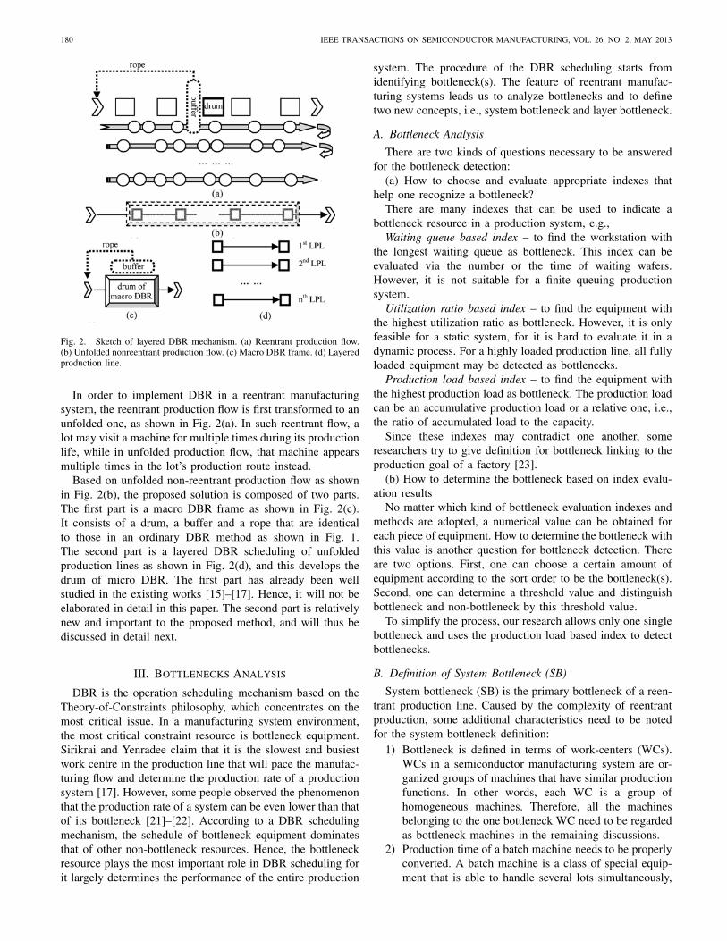
Fig. 2. Sketch of layered DBR mechanism. (a) Reentrant production flow.(b) Unfolded nonreentrant production flow. (c) Macro DBR frame. (d) Layeredproduction line.
In order to implement DBR in a reentrant manufacturingsystem, the reentrant production flow is first transformed to anunfolded one, as shown in Fig. 2(a). In such reentrant flow, alot may visit a machine for multiple times during its productionlife, while in unfolded production flow, that machine appearsmultiple times in the lot’s production route instead.
Based on unfolded non-reentrant production flow as shownin Fig. 2(b), the proposed solution is composed of two parts.The first part is a macro DBR frame as shown in Fig. 2(c).It consists of a drum, a buffer and a rope that are identicalto those in an ordinary DBR method as shown in Fig. 1.The second part is a layered DBR scheduling of unfoldedproduction lines as shown in Fig. 2(d), and this develops thedrum of micro DBR. The first part has already been wellstudied in the existing works [15]–[17]. Hence, it will not beelaborated in detail in this paper. The second part is relativelynew and important to the proposed method, and will thus bediscussed in detail next.
III. Bottlenecks Analysis
DBR is the operation scheduling mechanism based on theTheory-of-Constraints philosophy, which concentrates on themost critical issue. In a manufacturing system environment,the most critical constraint resource is bottleneck equipment.Sirikrai and Yenradee claim that it is the slowest and busiestwork centre in the production line that will pace the manufac-turing flow and determine the production rate of a productionsystem [17]. However, some people observed the phenomenonthat the production rate of a system can be even lower than thatof its bottleneck [21]–[22]. According to a DBR schedulingmechanism, the schedule of bottleneck equipment dominatesthat of other non-bottleneck resources. Hence, the bottleneckresource plays the most important role in DBR scheduling forit largely determines the performance of the entire production
system. The procedure of the DBR scheduling starts fromidentifying bottleneck(s). The feature of reentrant manufac-turing systems leads us to analyze bottlenecks and to definetwo new concepts, i.e., system bottleneck and layer bottleneck.
A. Bottleneck Analysis
There are two kinds of questions necessary to be answeredfor the bottleneck detection:
(a) How to choose and evaluate appropriate indexes thathelp one recognize a bottleneck?
There are many indexes that can be used to indicate abottleneck resource in a production system, e.g.,
Waiting queue based index – to find the workstation withthe longest waiting queue as bottleneck. This index can beevaluated via the number or the time of waiting wafers.However, it is not suitable for a finite queuing productionsystem.
Utilization ratio based index – to find the equipment withthe highest utilization ratio as bottleneck. However, it is onlyfeasible for a static system, for it is hard to evaluate it in adynamic process. For a highly loaded production line, all fullyloaded equipment may be detected as bottlenecks.
Production load based index – to find the equipment withthe highest production load as bottleneck. The production loadcan be an accumulative production load or a relative one, i.e.,the ratio of accumulated load to the capacity.
Since these indexes may contradict one another, someresearchers try to give definition for bottleneck linking to theproduction goal of a factory [23].
(b) How to determine the bottleneck based on index evalu-ation results
No matter which kind of bottleneck evaluation indexes andmethods are adopted, a numerical value can be obtained foreach piece of equipment. How to determine the bottleneck withthis value is another question for bottleneck detection. Thereare two options. First, one can choose a certain amount ofequipment according to the sort order to be the bottleneck(s).Second, one can determine a threshold value and distinguishbottleneck and non-bottleneck by this threshold value.
To simplify the process, our research allows only one singlebottleneck and uses the production load based index to detectbottlenecks.
B. Definition of System Bottleneck (SB)
System bottleneck (SB) is the primary bottleneck of a reen-trant production line. Caused by the complexity of reentrantproduction, some additional characteristics need to be notedfor the system bottleneck definition:
1) Bottleneck is defined in terms of work-centers (WCs).WCs in a semiconductor manufacturing system are or-ganized groups of machines that have similar productionfunctions. In other words, each WC is a group ofhomogeneous machines. Therefore, all the machinesbelonging to the one bottleneck WC need to be regardedas bottleneck machines in the remaining discussions.
2) Production time of a batch machine needs to be properlyconverted. A batch machine is a class of special equip-ment that is able to handle several lots simultaneously,
QIAO AND WU: LAYERED DRUM-BUFFER-ROPE BASED SCHEDULING OF REENTRANT MANUFACTURING SYSTEMS 181
consuming only one portion of production time. In orderto be consistent with the production time of a non-batchmachine, the production time of a batch machine needsto be divided by the batch number.
3) Dynamic machine breakdown is temporally not consid-ered in our current work. As pointed out by Wu andHui [24], the effective process time cannot be measuredunder the existence of time-based interruptions. Forfurther discussion on this topic please refer to [24]–[25].
To find SB, we adopt the accumulative production load asits evaluation index as follows.
Lh =1
μh
x∑
i=1
qi
y∑
j=1
θijh · tijh, h = 1, 2, · · · , H (1)
where Lh denotes the accumulative production load of WC-hwith the observation time range as mean life cycle time of theproduction flow; x is the number of product families; y is thenumber of production steps of the i#product family; qi is thenumber of product items in the i# product family; and θijh is acorrelation coefficient of equipment. It is 1 (0) if the jth stepof a product in the i# family can (not) be processed on WC-h.tijh expresses production time of the jth step of a product inthe i# family on WC-h. μh denotes the capacity of WC-h,which is the product of batch size (mh) of a batch machineand the quantity (nh) of machines in the WC. Mathematically,μh = mh × nh, where mh = 1 for a non-batch WC and mh >
1 for batch WC. H is the total number of WCs involved in areentrant manufacturing system.
Definition 1: System Bottleneck (SB): the work-center withthe highest accumulative production load in a reentrant pro-duction line, i.e.,
LB = max{L1, L2, . . . , LH }. (2)
To identify SB, we define only one system bottleneckfor a certain reentrant production line. Though there mayexist more than one WC satisfying (2), our work focuseson single SB discussion only, for it is encountered the mostin practice. Since system bottlenecks are defined in terms ofWCs, the detected system bottleneck actually means a groupof bottleneck machines with identical production capability.
C. Definition of Layer Bottleneck (LB)
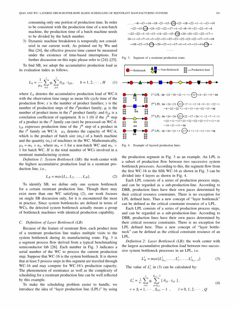
Because of the feature of reentrant flow, each product itemof a reentrant production line makes multiple visits to thesystem bottleneck during its manufacturing route. Fig. 3 isa segment process flow derived from a typical benchmarkingsemiconductor fab [26]. Each number in Fig. 3 indicates aserial number of the WC to process the current productionstep. Suppose that WC-16 is the system bottleneck. It is shownthat at least 5 process steps in this segment are traveled throughWC-16 and may compete for WC-16’s production capacity.The phenomenon of reentrance as well as the complexity ofscheduling for a reentrant production line can be well reflectedby this example.
To make the scheduling problem easier to handle, weintroduce the idea of “layer production line (LPL)” by using
Fig. 3. Segment of a reentrant production route.
Fig. 4. Example of layered production lines.
the production segment in Fig. 3 as an example. An LPL isa subset of production flow between two successive systembottleneck processes. According to this, the segment flow fromthe first WC-16 to the fifth WC-16 as shown in Fig. 3 can bedivided into 4 layers as shown in Fig. 4.
Each LPL consists of a series of production process steps,and can be regarded as a sub-production-line. According toDBR, production lines have their own paces determined bytheir critical resource constraints. There is no exception forLPL defined here. Thus a new concept of “layer bottleneck”can be defined as the critical constraint resource of a LPL.
Each LPL consists of a series of production process steps,and can be regarded as a sub-production-line. According toDBR, production lines have their own paces determined bytheir critical resource constraints. There is no exception forLPL defined here. Thus a new concept of “layer bottle-neck” can be defined as the critical constraint resource of anLPL.
Definition 2: Layer Bottleneck (LB): the work center withthe largest accumulative production load between two succes-sive system bottleneck processes in an LPL, i.e.
LlK = max{Ll
Sl+1, . . . , Ll
r, . . . , LlSl+1−1} (3)
The value of Llr in (3) can be calculated by:
Llr = 1
μr
x∑
i=1
qi
Sl+1−1∑
j=Sl+1
[ θijr · tijr ] ,
r = Sl + 1, · · · , Sl+1 − 1 , l = 0, 1, 2, · · · , Q
(4)
182 IEEE TRANSACTIONS ON SEMICONDUCTOR MANUFACTURING, VOL. 26, NO. 2, MAY 2013
Here, Llr is the accumulative production load of WC-r in
the lth LPL; Sl denotes the step number of a lot that visits theSB at the lth time in this step according to its production flow.Q is the total number of layers involved in the LPL. Othernotations in (4) are already explained in (1).
It is clear that an LB cannot be an SB by the definitions.SB is based on system-level production load calculation, whileLB based on local load calculation.
According to (3) and (4), LB of each LPL is detected. Inthis example, we assume the LBs of 1st to 4th LPL are WC-13,WC-22, WC-23 and WC-17 as circled in Fig. 4.
IV. Layered Scheduling Algorithm (LSA)
Both SB and LB are bottlenecks with characteristics ofhigh production load, high utilization and high competitionby production operations. After they are identified, the nextproblem is how to deal with the capacity allocation for them.This section presents the algorithms to solve it.
In addition to the DBR theory, different approaches areproposed to deal with the scheduling of bottleneck and non-bottleneck equipment. For the former, a detailed schedule,referred to as a drum, is found that specifies a starting time foreach operation at that equipment. The bottleneck schedule thatdetermines the beat or pace of the entire operation of a systemis most important since it can maximize system throughput bymaking full use of the system’s bottleneck resource. For thenon-bottleneck, detailed schedules are not necessary becauseit is supposed that they have more than enough capacity tokeep pace with the bottleneck. However, production fluctuationoccurring at non-bottleneck can disrupt the drum schedule.Buffer and rope mechanisms are thus designed to ensure thesubordination of all non-bottlenecks to the drum.
Based on the concept of SB and LB, a reentrant productionline is divided into multiple layers by SB denoting the criticalconstraint resource (CCR) in an entire production line, andeach LPL bears one LB denoting the CCR in a local LPL.Introduction of unfolded and layered production lines canbring some benefits for scheduling analysis. First, it eliminatesthe reentrant flow and debases the complexity of a schedulingproblem. Second, it enables problem decomposition such thateach LPL scheduling can be treated independently.
A. Principle of LSA
In the context of transformation from a reentrant productionline to an unfolded layered production line, a new layeredscheduling algorithm (LSA) based on DBR is proposed. Itsobjective is to generate a detailed schedule of system bot-tleneck, and thus solve the drum development problem of alayered production line.
LSA starts from building a layered production line for areentrant manufacturing system. After the original reentrantsystem is unfolded and decomposed, each LPL can be regardedas a common production line that can be scheduled via a DBRmethod. From this viewpoint, the start and end SB of a certainLPL (e.g. the first and second WC-h in the 1st LPL shown inFig. 4), are the release and the shipping point, while the LB
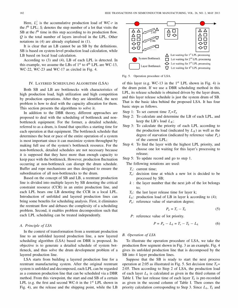
Fig. 5. Operation procedure of LSA.
of this layer (e.g. WC-13 in the 1st LPL shown in Fig. 4) isthe drum point. If we use a DBR scheduling method in thisLPL, its release schedule is obtained driven by the layer drum,and this layer release schedule is just the system drum of SB.That is the basic idea behind the proposed LSA. It has fourbasic steps as follows.Step 1: To set current time Ts=Tn
Step 2: To calculate and determine the LB of each LPL, andkeep the LB’s load LK;
Step 3: To calculate the priority of each LPL according tothe production load (indicated by LK) as well as thedegree of starvation (indicated by reference value Pu)of the current LPL;
Step 4: To find the layer with the highest LPL priority, andchoose one lot waiting for this layer’s processing torelease;
Step 5: To update record and go to step 1.The following notations are used:
Ts: current time;Tn: decision time at which a new lot is decided to be
processed by SB;k : the layer number that the next job of the lot belongs
to;Tk: the last layer release time for layer k;Lk: production load of LB in layer k according to (4);Pu: reference value of starvation degree;
Pu = Ts − Tk (5)
P: reference value of lot priority.
P = Pu − Lk = Ts − Tk − Lk (6)
B. Operation of LSA
To illustrate the operation procedure of LSA, we take theproduction flow segment shown in Fig. 3 as an example. Fig. 4gives its unfolded production line that is decomposed by theSB into 4 layer production lines.
Suppose that the SB is ready to start the next processoperation at 2:05 as illustrated in Fig. 5. Set decision time Tn=2:05. Then according to Step 2 of LSA, the production loadof each layer Lk is calculated as given in the third column ofTable I. The last release time of each layer Tk is pre-recordedas given in the second column of Table I. Then comes thepriority calculation corresponding to Step 3. Since Lk, Tk and
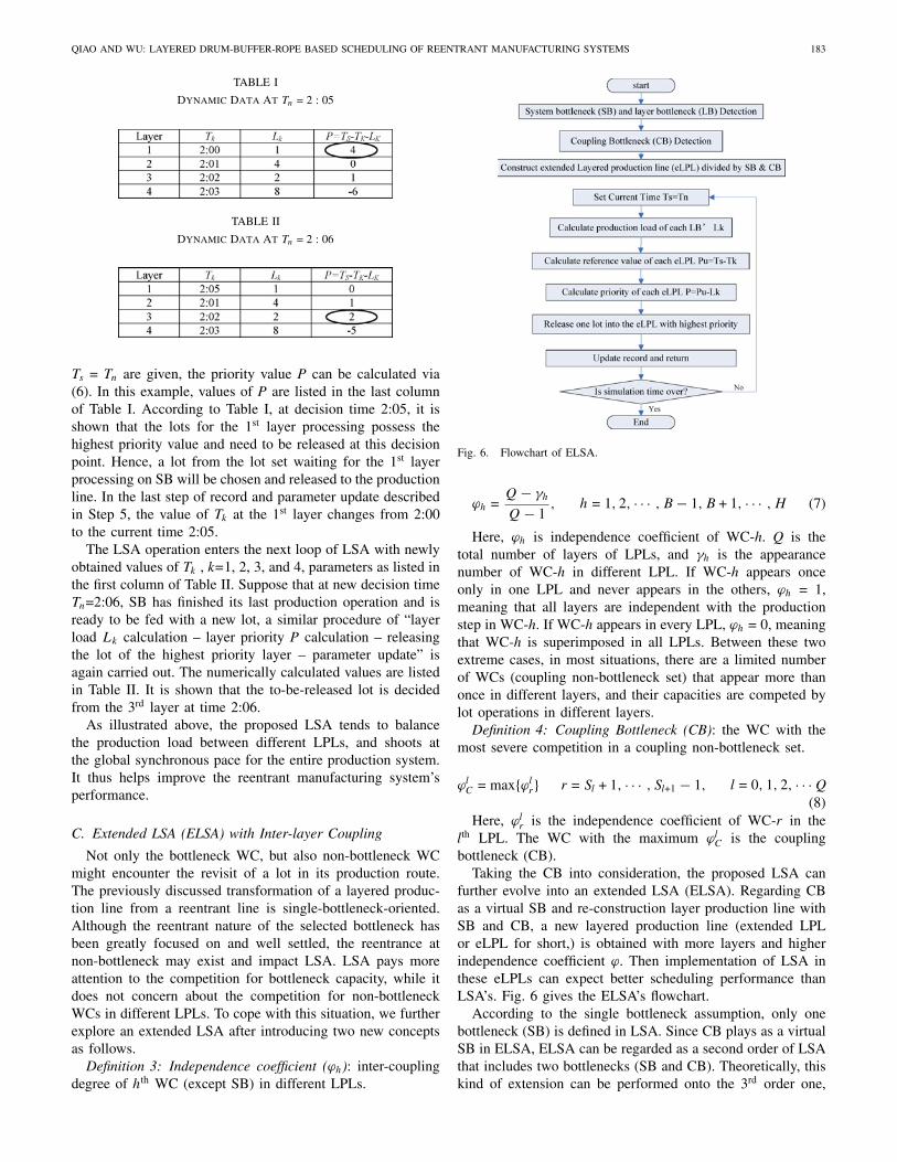
QIAO AND WU: LAYERED DRUM-BUFFER-ROPE BASED SCHEDULING OF REENTRANT MANUFACTURING SYSTEMS 183
TABLE I
Dynamic Data At Tn = 2 : 05
TABLE II
Dynamic Data At Tn = 2 : 06
Ts = Tn are given, the priority value P can be calculated via(6). In this example, values of P are listed in the last columnof Table I. According to Table I, at decision time 2:05, it isshown that the lots for the 1st layer processing possess thehighest priority value and need to be released at this decisionpoint. Hence, a lot from the lot set waiting for the 1st layerprocessing on SB will be chosen and released to the productionline. In the last step of record and parameter update describedin Step 5, the value of Tk at the 1st layer changes from 2:00to the current time 2:05.
The LSA operation enters the next loop of LSA with newlyobtained values of Tk , k=1, 2, 3, and 4, parameters as listed inthe first column of Table II. Suppose that at new decision timeTn=2:06, SB has finished its last production operation and isready to be fed with a new lot, a similar procedure of “layerload Lk calculation – layer priority P calculation – releasingthe lot of the highest priority layer – parameter update” isagain carried out. The numerically calculated values are listedin Table II. It is shown that the to-be-released lot is decidedfrom the 3rd layer at time 2:06.
As illustrated above, the proposed LSA tends to balancethe production load between different LPLs, and shoots atthe global synchronous pace for the entire production system.It thus helps improve the reentrant manufacturing system’sperformance.
C. Extended LSA (ELSA) with Inter-layer Coupling
Not only the bottleneck WC, but also non-bottleneck WCmight encounter the revisit of a lot in its production route.The previously discussed transformation of a layered produc-tion line from a reentrant line is single-bottleneck-oriented.Although the reentrant nature of the selected bottleneck hasbeen greatly focused on and well settled, the reentrance atnon-bottleneck may exist and impact LSA. LSA pays moreattention to the competition for bottleneck capacity, while itdoes not concern about the competition for non-bottleneckWCs in different LPLs. To cope with this situation, we furtherexplore an extended LSA after introducing two new conceptsas follows.
Definition 3: Independence coefficient (ϕh): inter-couplingdegree of hth WC (except SB) in different LPLs.
Fig. 6. Flowchart of ELSA.
ϕh =Q − γh
Q − 1, h = 1, 2, · · · , B − 1, B + 1, · · · , H (7)
Here, ϕh is independence coefficient of WC-h. Q is thetotal number of layers of LPLs, and γh is the appearancenumber of WC-h in different LPL. If WC-h appears onceonly in one LPL and never appears in the others, ϕh = 1,meaning that all layers are independent with the productionstep in WC-h. If WC-h appears in every LPL, ϕh = 0, meaningthat WC-h is superimposed in all LPLs. Between these twoextreme cases, in most situations, there are a limited numberof WCs (coupling non-bottleneck set) that appear more thanonce in different layers, and their capacities are competed bylot operations in different layers.
Definition 4: Coupling Bottleneck (CB): the WC with themost severe competition in a coupling non-bottleneck set.
ϕlC = max{ϕl
r} r = Sl + 1, · · · , Sl+1 − 1, l = 0, 1, 2, · · · Q(8)
Here, ϕlr is the independence coefficient of WC-r in the
lth LPL. The WC with the maximum ϕlC is the coupling
bottleneck (CB).Taking the CB into consideration, the proposed LSA can
further evolve into an extended LSA (ELSA). Regarding CBas a virtual SB and re-construction layer production line withSB and CB, a new layered production line (extended LPLor eLPL for short,) is obtained with more layers and higherindependence coefficient ϕ. Then implementation of LSA inthese eLPLs can expect better scheduling performance thanLSA’s. Fig. 6 gives the ELSA’s flowchart.
According to the single bottleneck assumption, only onebottleneck (SB) is defined in LSA. Since CB plays as a virtualSB in ELSA, ELSA can be regarded as a second order of LSAthat includes two bottlenecks (SB and CB). Theoretically, thiskind of extension can be performed onto the 3rd order one,
184 IEEE TRANSACTIONS ON SEMICONDUCTOR MANUFACTURING, VOL. 26, NO. 2, MAY 2013
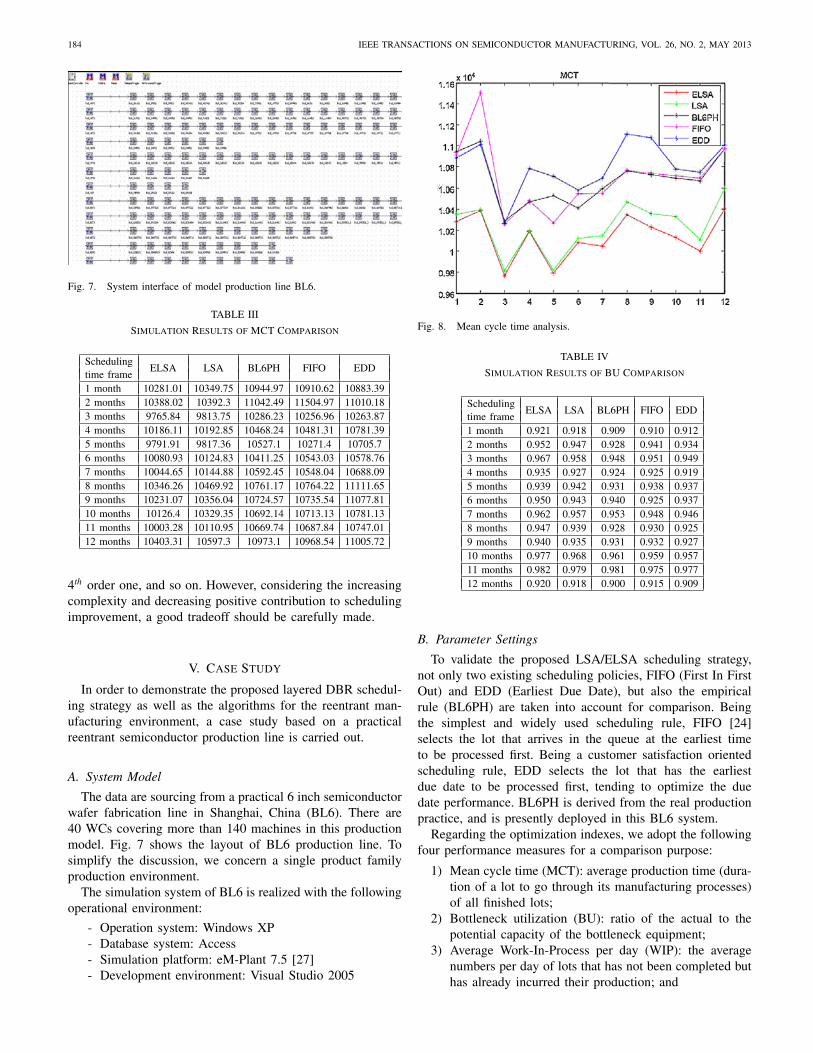
Fig. 7. System interface of model production line BL6.
TABLE III
Simulation Results of MCT Comparison
SchedulingELSA LSA BL6PH FIFO EDD
time frame1 month 10281.01 10349.75 10944.97 10910.62 10883.392 months 10388.02 10392.3 11042.49 11504.97 11010.183 months 9765.84 9813.75 10286.23 10256.96 10263.874 months 10186.11 10192.85 10468.24 10481.31 10781.395 months 9791.91 9817.36 10527.1 10271.4 10705.76 months 10080.93 10124.83 10411.25 10543.03 10578.767 months 10044.65 10144.88 10592.45 10548.04 10688.098 months 10346.26 10469.92 10761.17 10764.22 11111.659 months 10231.07 10356.04 10724.57 10735.54 11077.8110 months 10126.4 10329.35 10692.14 10713.13 10781.1311 months 10003.28 10110.95 10669.74 10687.84 10747.0112 months 10403.31 10597.3 10973.1 10968.54 11005.72
4th order one, and so on. However, considering the increasingcomplexity and decreasing positive contribution to schedulingimprovement, a good tradeoff should be carefully made.
V. Case Study
In order to demonstrate the proposed layered DBR schedul-ing strategy as well as the algorithms for the reentrant man-ufacturing environment, a case study based on a practicalreentrant semiconductor production line is carried out.
A. System Model
The data are sourcing from a practical 6 inch semiconductorwafer fabrication line in Shanghai, China (BL6). There are40 WCs covering more than 140 machines in this productionmodel. Fig. 7 shows the layout of BL6 production line. Tosimplify the discussion, we concern a single product familyproduction environment.
The simulation system of BL6 is realized with the followingoperational environment:
- Operation system: Windows XP- Database system: Access- Simulation platform: eM-Plant 7.5 [27]- Development environment: Visual Studio 2005
Fig. 8. Mean cycle time analysis.
TABLE IV
Simulation Results of BU Comparison
SchedulingELSA LSA BL6PH FIFO EDD
time frame1 month 0.921 0.918 0.909 0.910 0.9122 months 0.952 0.947 0.928 0.941 0.9343 months 0.967 0.958 0.948 0.951 0.9494 months 0.935 0.927 0.924 0.925 0.9195 months 0.939 0.942 0.931 0.938 0.9376 months 0.950 0.943 0.940 0.925 0.9377 months 0.962 0.957 0.953 0.948 0.9468 months 0.947 0.939 0.928 0.930 0.9259 months 0.940 0.935 0.931 0.932 0.92710 months 0.977 0.968 0.961 0.959 0.95711 months 0.982 0.979 0.981 0.975 0.97712 months 0.920 0.918 0.900 0.915 0.909
B. Parameter Settings
To validate the proposed LSA/ELSA scheduling strategy,not only two existing scheduling policies, FIFO (First In FirstOut) and EDD (Earliest Due Date), but also the empiricalrule (BL6PH) are taken into account for comparison. Beingthe simplest and widely used scheduling rule, FIFO [24]selects the lot that arrives in the queue at the earliest timeto be processed first. Being a customer satisfaction orientedscheduling rule, EDD selects the lot that has the earliestdue date to be processed first, tending to optimize the duedate performance. BL6PH is derived from the real productionpractice, and is presently deployed in this BL6 system.
Regarding the optimization indexes, we adopt the followingfour performance measures for a comparison purpose:
1) Mean cycle time (MCT): average production time (dura-tion of a lot to go through its manufacturing processes)of all finished lots;
2) Bottleneck utilization (BU): ratio of the actual to thepotential capacity of the bottleneck equipment;
3) Average Work-In-Process per day (WIP): the averagenumbers per day of lots that has not been completed buthas already incurred their production; and
QIAO AND WU: LAYERED DRUM-BUFFER-ROPE BASED SCHEDULING OF REENTRANT MANUFACTURING SYSTEMS 185
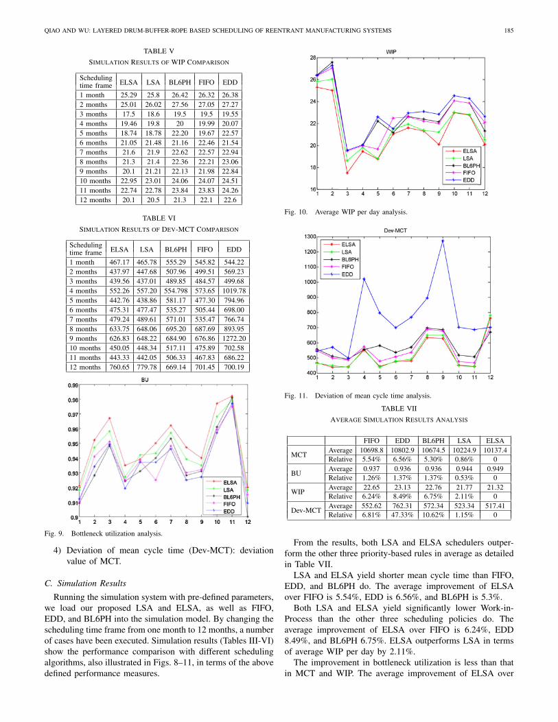
TABLE V
Simulation Results of WIP Comparison
SchedulingELSA LSA BL6PH FIFO EDDtime frame
1 month 25.29 25.8 26.42 26.32 26.382 months 25.01 26.02 27.56 27.05 27.273 months 17.5 18.6 19.5 19.5 19.554 months 19.46 19.8 20 19.99 20.075 months 18.74 18.78 22.20 19.67 22.576 months 21.05 21.48 21.16 22.46 21.547 months 21.6 21.9 22.62 22.57 22.948 months 21.3 21.4 22.36 22.21 23.069 months 20.1 21.21 22.13 21.98 22.8410 months 22.95 23.01 24.06 24.07 24.5111 months 22.74 22.78 23.84 23.83 24.2612 months 20.1 20.5 21.3 22.1 22.6
TABLE VI
Simulation Results of Dev-MCT Comparison
SchedulingELSA LSA BL6PH FIFO EDDtime frame
1 month 467.17 465.78 555.29 545.82 544.222 months 437.97 447.68 507.96 499.51 569.233 months 439.56 437.01 489.85 484.57 499.684 months 552.26 557.20 554.798 573.65 1019.785 months 442.76 438.86 581.17 477.30 794.966 months 475.31 477.47 535.27 505.44 698.007 months 479.24 489.61 571.01 535.47 766.748 months 633.75 648.06 695.20 687.69 893.959 months 626.83 648.22 684.90 676.86 1272.2010 months 450.05 448.34 517.11 475.89 702.5811 months 443.33 442.05 506.33 467.83 686.2212 months 760.65 779.78 669.14 701.45 700.19
Fig. 9. Bottleneck utilization analysis.
4) Deviation of mean cycle time (Dev-MCT): deviationvalue of MCT.
C. Simulation Results
Running the simulation system with pre-defined parameters,we load our proposed LSA and ELSA, as well as FIFO,EDD, and BL6PH into the simulation model. By changing thescheduling time frame from one month to 12 months, a numberof cases have been executed. Simulation results (Tables III-VI)show the performance comparison with different schedulingalgorithms, also illustrated in Figs. 8–11, in terms of the abovedefined performance measures.
Fig. 10. Average WIP per day analysis.
Fig. 11. Deviation of mean cycle time analysis.
TABLE VII
Average Simulation Results Analysis
FIFO EDD BL6PH LSA ELSA
MCTAverage 10698.8 10802.9 10674.5 10224.9 10137.4Relative 5.54% 6.56% 5.30% 0.86% 0
BUAverage 0.937 0.936 0.936 0.944 0.949Relative 1.26% 1.37% 1.37% 0.53% 0
WIPAverage 22.65 23.13 22.76 21.77 21.32Relative 6.24% 8.49% 6.75% 2.11% 0
Dev-MCTAverage 552.62 762.31 572.34 523.34 517.41Relative 6.81% 47.33% 10.62% 1.15% 0
From the results, both LSA and ELSA schedulers outper-form the other three priority-based rules in average as detailedin Table VII.
LSA and ELSA yield shorter mean cycle time than FIFO,EDD, and BL6PH do. The average improvement of ELSAover FIFO is 5.54%, EDD is 6.56%, and BL6PH is 5.3%.
Both LSA and ELSA yield significantly lower Work-in-Process than the other three scheduling policies do. Theaverage improvement of ELSA over FIFO is 6.24%, EDD8.49%, and BL6PH 6.75%. ELSA outperforms LSA in termsof average WIP per day by 2.11%.
The improvement in bottleneck utilization is less than thatin MCT and WIP. The average improvement of ELSA over
186 IEEE TRANSACTIONS ON SEMICONDUCTOR MANUFACTURING, VOL. 26, NO. 2, MAY 2013
FIFO, EDD, BL6PH, and LSA are 1.26%, 1.37%, 1.37%, and0.53% respectively.
VI. Conclusion
Drum-buffer-rope (DBR) is one of the best productioncontrol methods and has already gained successful applicationsin many industries. For a class of complex manufacturingsystems with reentrant production flow, this work for the firsttime proposes a layered DBR scheduling strategy. With thenewly introduced concepts of system bottleneck and layerbottleneck, a layered scheduling algorithm (LSA) for a reen-trant production line is developed. To deal with the couplingbetween different production layers, an extended LSA (ELSA)is presented. Our extensive simulation studies indicate thatthe layered DBR scheduling mechanism with both LSA andELSA can lead to significant improvement in terms of meanproduct cycle time and Work-in-Process per day than empiricalscheduling rule as well as two standard ones: First In FirstOut and Earliest Due Date. Their validity is also shown viadeviation of MCT and bottleneck utilization improvements bytheir deployment. Since the coupling factor is further takeninto consideration by ELSA, it performs better than LSA. Itis concluded that the proposed layered DBR-based schedulingapproach is effective for a reentrant manufacturing system.
The LSA and ELSA methods discussed in this paper canbe considered as the first-order algorithm and second-orderalgorithm, respectively. Though given simulation results showthat the performance of ELSA is better than that of LSA, itremains unknown if the higher order algorithms can lead tobetter solutions. Therefore, further research is needed to decidea good tradeoff point by balancing their contribution to per-formance and computational cost. Further issues worthy to beaddressed also include the computational complexity analysisof the proposed algorithms, the comparison and evaluationof different methods for bottleneck detection, and dynami-cally changing bottleneck(s). The actual implementation andtest of the proposed strategy in semiconductor plants shouldbe sought.
Acknowledgement
The authors would like to thank X. Ding, Y. Dai, and X. Yufor their work on this project. The authors are also gratefulto the Associate Editor and reviewers for their constructivecomments.
References
[1] D. Y. Liao, M. D. Jeng, and M. C. Zhou, “Petri net modeling andLagrangian relaxation approach to vehicle scheduling in 300 mm semi-conductor manufacturing,” IEEE Trans. Syst., Man, Cybern., C, vol. 37,no. 4, pp. 504–516, Jul. 2007.
[2] Y. Qiao, N. Wu, and M. C. Zhou, “Modeling and analysis of dual-armcluster tools for wafer fabrication with revisiting,” in Proc. IEEE Int.Conf. Autom. Sci. Eng., Aug. 2011, pp. 90–95.
[3] C. T. Chen and Y. C. Chuang, “An intelligent run-to-run control strategyfor chemical-mechanical polishing processes,” IEEE Trans. Semicond.Manuf., vol. 23, no. 1, pp. 109–20, Feb. 2010.
[4] L. Li and F. Qiao, “Integrated intelligent optimized dynamic schedulingof semiconductor fabrication facilities,” in Proc. IEEE Int. Conf. Autom.Logistics, Aug. 2010, pp. 690–695.
[5] H. H. Xiong and M. C. Zhou, “Scheduling of semiconductor test facilityvia Petri nets and hybrid heuristic search,” IEEE Trans. Semicond.Manuf., vol. 11, no. 3, pp. 384–393, Aug. 1998.
[6] N. Wu and M. C. Zhou, “Schedulability analysis and optimal schedulingof dual-arm cluster tools with residency time constraint and activity timevariation,” IEEE Trans. Autom. Sci. Eng., vol. 9, no. 1, pp. 203–209, Jan.2012.
[7] D. E. Akyol and G. M. Bayhan, “A review on evolution of productionscheduling with neural networks,” Comput. Ind. Eng., vol. 53, no. 1, pp.95–122, 2007.
[8] N. Wu, C. Chu, F. Chu, and M. C. Zhou, “A Petri net method forschedulability and scheduling problems in single-arm cluster tools withwafer residency time constraints,” IEEE Trans. Semicond. Manuf., vol.21, no. 2, pp. 224–237, May 2008.
[9] N. Wu and M. C. Zhou, “Modeling, analysis and control of dual-armcluster tools with residency time constraint and activity time variationvia Petri nets,” IEEE Trans. Autom. Sci. Eng., vol. 9, no. 2, pp. 446–454,Apr. 2012.
[10] R. M. Dabbas and J. W. Fowler, “A new scheduling approach usingcombined dispatching criteria in wafer fabs,” IEEE Trans. Semicond.Manuf., vol. 16, no. 3, pp. 501–510, Aug. 2003.
[11] Z.-T. Wang, Q.-D. Wu, and F. Qiao, “A lot dispatching strategy inte-grating WIP management and wafer start control,” IEEE Trans. Autom.Sci. Eng., vol. 4, no. 4, pp. 579–583, Oct. 2007.
[12] J. A. Ramirez-Hernandez, J. Crabtree, X. Yao, E. Fernandez, M. C.Fu, M. Janakiram, S. I. Marcus, M. O’Connor and N. Patel, “Optimalpreventive maintenance scheduling in semiconductor manufacturing sys-tems: Software tool and simulation case studies,” IEEE Trans. Semicond.Manuf., vol. 23, no. 3, pp. 477–489, Aug. 2010.
[13] E. M. Goldratt, The Goal. Groton-on-Hudson, NY, USA: North RiverPress, 1986.
[14] V. Daniel and R. Guide, Jr., “Scheduling with priority dispatching rulesand drum-buffer-rope in a recoverable manufacturing system,” Int. J.Prod. Econ., vol. 53, no. 1, pp. 101–116, 1997.
[15] K. Woo, S. Park, and S. Fujimura, “Real-time buffer managementmethod for DBR scheduling,” Int. J. Manuf. Technol. Manage., vol. 16,nos. 1–2, pp. 42–57, 2009.
[16] S. S. Chakravorty, “An evaluation of the DBR control mechanismin a job shop environment,” Omega, vol. 29, no. 4, pp. 335–342,2001.
[17] V. Sirikrai and P. Yenradee, “Modified drum-buffer-rope schedul-ing mechanism for a non-identical parallel machine flow shop withprocessing-time variation,” Int. J. Prod. Res., vol. 44, no. 17, pp. 3509–3531, 2006.
[18] E. Schragenheim and B. Ronen, “Drum-buffer-rope shop floor con-trol, Prod. Inventory Manage. J., vol. 31, no. 3, pp. 18–23,1990.
[19] D. Kayton, “Using the theory of constraints’ production application ina semiconductor fab with a reentrant bottleneck,” in Proc. IEEE/CPMTInt. Electron. Manuf. Technol. Symp., Oct. 1998, pp. 352–357.
[20] H.-H. Wu and M.-L. Yeh, “A DBR scheduling method for manufacturingenvironments with bottleneck re-entrant flows,” Int. J. Prod. Res., vol.44, no. 5, pp. 883–902, 2006.
[21] P. R. Kumar and T. I. Seidman, “Dynamic instabilities and stabilizationmethods in distributed real-time scheduling of manufacturing systems,”IEEE Trans. Automatic Control, vol. 35, no. 3, pp. 289–298, Mar.1990.
[22] S. H. Lu and P. R. Kumar, “Distributed scheduling based on due datesand buffer priorities,” IEEE Trans. Automatic Control, vol. 36, no. 12,pp. 1406–1416, Dec. 1991.
[23] K. Wu, “An examination of variability and its basic properties for afactory,” IEEE Trans. Semicond. Manuf., vol. 18, no. 1, pp. 214–221,Feb. 2005.
[24] K. Wu and K. Hui, “The determination and indetermination of servicetimes in manufacturing systems,” IEEE Trans. Semicond. Manuf., vol.21, no. 1, pp. 72–82, Feb. 2008.
[25] K. Wu, L. McGinnis, and B. Zwart, “Queueing models for a singlemachine subject to multiple types of interruptions,” IIE Trans., vol. 43,no. 10, pp. 753–759, 2011.
[26] L. M. Wein, “Scheduling semiconductor wafer fabrication,” IEEE Trans.Semicond. Manuf., vol. 1, no. 3, pp. 115–130, Aug. 1988.
[27] eM-Plant User’s Manual, version 7.5, Tecnomatix Gmbh, Stuttgart,Germany, 2005.
QIAO AND WU: LAYERED DRUM-BUFFER-ROPE BASED SCHEDULING OF REENTRANT MANUFACTURING SYSTEMS 187
Fei Qiao (M’99–SM’08) was born in Anhui, China,in 1967. She received the B.S. and M.S. degreesfrom the Department of Electrical Engineering,Tongji University, Shanghai, China, in 1990 and1993, respectively, and the Ph.D. degree from theSchool of Economics and Management, Tongji Uni-versity, in 1997.
She is currently a Professor at the School of Elec-tronics and Information Engineering, Tongji Univer-sity. Her current research interests include planningand scheduling of complex manufacturing system,
energy efficiency manufacturing, modeling and optimization, and systemintegration.
Qidi Wu (M’85–SM’92) received the B.S. andM.S. degrees from the Department of ElectricalEngineering and the Department of Mechanical En-gineering, Tsinghua University, Beijing, China, in1970 and 1981, respectively, and the Ph.D. degreefrom the Department of Electrical Engineering, Fed-eral Institute of Technology, Zurich, Switzerland, in1986.
In 1986, she joined Tongji University, Shanghai,China, as a Professor at the School of Electronicsand Information Engineering and the School of
Economics and Management. She was the President of Tongji University from1995 to 2003. Her current research interests include planning and schedulingof complex manufacturing systems, intelligent control theory and engineering,system engineering, and engineering management.
Dr. Wu is currently the Chairperson of the National Committee of Engi-neering Education Accreditation of China, the Chair of the InformationizationExpert Committee of Shanghai Government and a Standing Member of theChinese Association of Automation.