Embed Size (px)
Citation preview

Late-Quaternary Landscape Dynamics in the Iberian Peninsula
and Balearic Islands
José Pedro Rodrigues Tarroso Gomes
Porto


Late-Quaternary Landscape Dynamics in the Iberian Peninsula
and Balearic Islands
José Pedro Rodrigues Tarroso Gomes
Porto
a proposal submitted in partial fulfi llment of the degree of Master of Sciences
to Faculdade de Ciências da Universidade do Porto
Master in Biodiversity and Genetic Resources

ii |

| iii
To the memory of my mother.

iv |

| v
AcknowledgementsSince the beginning of this masters project, many people have shown their interest and were funda-
mental to its completion.
In the fi rst place I have to mention my supervisor Professor Paulo Célio who suggested the
thesis theme and who believed I would be able to execute it. It was a long walk to achieve the fi nal
result and I hope that this work can, at least, be at the level of his expectations. One person without
whom this thesis would be entirely (or even more) impossible was José Carlos Brito. I am immensely
thankful for his guidance, suggestions and reviews from the last glacial maximum until the present
time!
Th e support of my family was extremely important during the development of this manu-
script. My father, who was always present with great sense of humour, gave me all the support I
needed. My brother, sister and grandparents were permanently present as well. It is strange to be
surrounded day after day by biologists, geneticists and all source of statistical analyses aiming at the
most basic logic thinking of the scientifi c method and then to feel the peculiar genetic bound like I
feel with them. I also would like to mention Helena and her children for the kind support they gave.
I am indebted to my friends Pedro and Sofi a: you are just like a family. You have the ability to
make me think that I am capable to achieve good results and our conversations are always so prolifi c
in both fi elds of science and art. Without all the knowledge I have stolen from you, this work would
never be possible. I also would not understand anything about 14C without Elin’s help. I am pleased
to be her friend and grateful to all her endless questions! Some of the best conversations I ever had
were with Sara and all her lunacy: thank you for being present and I hope biology didn’t make any
harm to you! Adriano, you are a good friend. You patiently listened all I said in the best and worst
moments throughout this work and you always had something to say that was, at least, unexpected,
however bright! I am especially thankful to Fátima for all her support and concern with me and with
my work.
It was gratifying to receive the support of some colleagues at work. Th e support of my “lab”
friends Fernando Lima, Nuno Queiroz and Pedro Ribeiro was completely indispensable. You are
great scientists and friends and I appreciated all the belief in me and the help you gave me since the
beginning. And also all the laughs! Furthermore, I am grateful for the opportunities you gave me to
work with you. I could not forget Raquel Xavier and her superior skills in friendship! I am also
thankful to my friends Joana Abrantes, who lent me some distracting literature, and Diana. Miguel

vi |
Carretero became a good friend after all this time I worked at CIBIO, and I have learnt a lot with
him. I am also thankful to Catarina Rato and to the newest international friends, Anna and Jay, who
provided good moments during the obscure period of writing a thesis!
One of the everlasting friends I made even before I began working at CIBIO was Catarina
Ferreira. Th ank you for all your support and the friendship revealed every time we meet. I have
enjoyed working with Joana and Claudia and I am thankful for their great friendship. Francisco
Álvares was extremely helpful with all the bibliography he lent me just because he saw a probable
link to my work. He always provided good moments and laughs in the workplace. I am especially
thankful to him and also to Neftalí Sillero due to the trust he deposited in me all this time, the
friendship and those hard to fi nd papers he dug up in Salamanca. He was also the fi rst person with
whom I shared a offi ce in Vairão and, since then, a good mood was the tone with all the colleagues
there, to whom I am indebted, especially to Silvia. I am also thankful to João Torres, with whom I
had productive dialogues about GIS (among other more interesting subjects), and Hélder Freitas.
Both have been good friends since the beginning of this masters. I also have to mention my gratitude
to Paulo Alves for his friendship and some tips about vegetation in the Iberian Peninsula and to
Professor João Honrado for revealing confi dence in my work, interest in the subject and the provided
literature. Finally, all my colleagues at CIBIO were responsible for the fact that this thesis reached its
end, with the manifested interest and support given.
I bootstrapped these people a huge number of times along with some other else I am forget-
ting, as you were so many to mention here. I reached one hundred percent confi dence that this work
would never be possible without all of you. Th ank you all.

| vii
Table of ContentsResumo . . . . . . . . . . . . . . . . . . . . . . . . . . . . . . . . . . . . . . . . . . . . . . . . . . . . . . . . . . . . . . . . . . . . . . . . xi
Abstract . . . . . . . . . . . . . . . . . . . . . . . . . . . . . . . . . . . . . . . . . . . . . . . . . . . . . . . . . . . . . . . . . . . . . . . xiii
1 Introduction . . . . . . . . . . . . . . . . . . . . . . . . . . . . . . . . . . . . . . . . . . . . . . . . . . . . . . . . . . . . . . . . . . . . 1
1.1 Biogeography . . . . . . . . . . . . . . . . . . . . . . . . . . . . . . . . . . . . . . . . . . . . . . . . . . . . . . . . . . . . . . . . . . . . . . . . 2
1.2 Climatic Oscillations . . . . . . . . . . . . . . . . . . . . . . . . . . . . . . . . . . . . . . . . . . . . . . . . . . . . . . . . . . . . . . . . . . 4
1.3 Reconstruction of past landscapes . . . . . . . . . . . . . . . . . . . . . . . . . . . . . . . . . . . . . . . . . . . . . . . . . . . . . . . . 6
1.4 GIS in past vegetation reconstructions . . . . . . . . . . . . . . . . . . . . . . . . . . . . . . . . . . . . . . . . . . . . . . . . . . . . 8
1. 5 Objectives . . . . . . . . . . . . . . . . . . . . . . . . . . . . . . . . . . . . . . . . . . . . . . . . . . . . . . . . . . . . . . . . . . . . . . . . . 10
2 Data and Methods . . . . . . . . . . . . . . . . . . . . . . . . . . . . . . . . . . . . . . . . . . . . . . . . . . . . . . . . . . . . . .11
2.1 Study Area . . . . . . . . . . . . . . . . . . . . . . . . . . . . . . . . . . . . . . . . . . . . . . . . . . . . . . . . . . . . . . . . . . . . . . . . 11
2.2 Dataset . . . . . . . . . . . . . . . . . . . . . . . . . . . . . . . . . . . . . . . . . . . . . . . . . . . . . . . . . . . . . . . . . . . . . . . . . . . 12
2.3 Biomization procedure . . . . . . . . . . . . . . . . . . . . . . . . . . . . . . . . . . . . . . . . . . . . . . . . . . . . . . . . . . . . . . . 16
2.4 Data visualization and analysis . . . . . . . . . . . . . . . . . . . . . . . . . . . . . . . . . . . . . . . . . . . . . . . . . . . . . . . . 18
3 Results. . . . . . . . . . . . . . . . . . . . . . . . . . . . . . . . . . . . . . . . . . . . . . . . . . . . . . . . . . . . . . . . . . . . . . . .21
3.1 Distribution of plant genera . . . . . . . . . . . . . . . . . . . . . . . . . . . . . . . . . . . . . . . . . . . . . . . . . . . . . . . . . . . 21
3.2 Distribution of Plant Functional Types . . . . . . . . . . . . . . . . . . . . . . . . . . . . . . . . . . . . . . . . . . . . . . . . . . 32
3.3 Distribution of Biomes . . . . . . . . . . . . . . . . . . . . . . . . . . . . . . . . . . . . . . . . . . . . . . . . . . . . . . . . . . . . . . . 33
3.4 Relationships between Biomes and environmental conditions . . . . . . . . . . . . . . . . . . . . . . . . . . . . . . . . . 36
3.5 Distribution of persistence areas of plant genera . . . . . . . . . . . . . . . . . . . . . . . . . . . . . . . . . . . . . . . . . . . 37
4 Discussion . . . . . . . . . . . . . . . . . . . . . . . . . . . . . . . . . . . . . . . . . . . . . . . . . . . . . . . . . . . . . . . . . . . .39
4.1 Correlations with climate data . . . . . . . . . . . . . . . . . . . . . . . . . . . . . . . . . . . . . . . . . . . . . . . . . . . . . . . . . 41
4.2 Comparing independent past landscape reconstructions . . . . . . . . . . . . . . . . . . . . . . . . . . . . . . . . . . . . . 45
4.3 Congruence with phylogenetic reconstructions . . . . . . . . . . . . . . . . . . . . . . . . . . . . . . . . . . . . . . . . . . . . . 48
4.4 Parallelism between fauna and fl ora refugia . . . . . . . . . . . . . . . . . . . . . . . . . . . . . . . . . . . . . . . . . . . . . . . 50
5 Conclusions . . . . . . . . . . . . . . . . . . . . . . . . . . . . . . . . . . . . . . . . . . . . . . . . . . . . . . . . . . . . . . . . . . .53
6 References . . . . . . . . . . . . . . . . . . . . . . . . . . . . . . . . . . . . . . . . . . . . . . . . . . . . . . . . . . . . . . . . . . . . .55
Appendices . . . . . . . . . . . . . . . . . . . . . . . . . . . . . . . . . . . . . . . . . . . . . . . . . . . . . . . . . . . . . . . . . . . . .67
Appendix I - Biome affi nity scores by sampled site . . . . . . . . . . . . . . . . . . . . . . . . . . . . . . . . . . . . . . . . . . . . 69
Appendix II – Script for interpolating affi nity surfaces . . . . . . . . . . . . . . . . . . . . . . . . . . . . . . . . . . . . . . . . . 71
Appendix III – Script for classify Biomes . . . . . . . . . . . . . . . . . . . . . . . . . . . . . . . . . . . . . . . . . . . . . . . . . . . 73

viii |
Appendix IV – Script for calculating correlations between maps . . . . . . . . . . . . . . . . . . . . . . . . . . . . . . . . . 75
Appendix V – Script for smoothing rasters . . . . . . . . . . . . . . . . . . . . . . . . . . . . . . . . . . . . . . . . . . . . . . . . . . 79
Appendix VI – Script for converting ascii fi les . . . . . . . . . . . . . . . . . . . . . . . . . . . . . . . . . . . . . . . . . . . . . . 81
Appendix VII – Script for masking rasters . . . . . . . . . . . . . . . . . . . . . . . . . . . . . . . . . . . . . . . . . . . . . . . . . . 83
Appendix VIII – Script for classifying rasters . . . . . . . . . . . . . . . . . . . . . . . . . . . . . . . . . . . . . . . . . . . . . . . . 85
Appendix IX – Script for exporting maps . . . . . . . . . . . . . . . . . . . . . . . . . . . . . . . . . . . . . . . . . . . . . . . . . . . 87

| ix

x |

| xi
ResumoO clima no planeta ao longo do fi m do Pleistocénico e durante todo o Holocénico foi instável, vari-
ando entre o frio extremo do último máximo glaciar (LGM) até períodos de aquecimento intenso.
Estas ocilações no clima suscitaram ciclos de contracção e expensão na distribuição da vida na Terra.
As temperaturas adversas do LGM concentraram a diversidade biológica em áreas de refúgio, locali-
zadas em latitudes inferiores e com um clima mais ameno, possibilitando eventos de especiação. No
sul da Europa, as penínsulas Ibérica, Itálica e Balcânica, são reconhecidas como áreas de refúgio para
várias espécies. Deste modo, a Península Ibérica confi gura-se como um local de extrema importância
para a análise de padrões paleogeográfi cos na distribuição da fauna e fl ora.
No presente trabalho é estudada a dinâmica da vegetação na Península Ibérica e ilhas
Baleares durante o período temporal entre 15 até 1 ky BP. Como estiveram distribuídos alguns
géneros vegetais e Tipos Funcionais de Plantas (PFT) durante o período em estudo? Qual era a área
ocupada pelos vários Biomas e a sua relação com as oscilações na temperatura? Para responder a
estas questões foram analisadas as presenças de fósseis de pólen dos géneros Alnus, Betula, Castanea, Fagus, Olea, Pistacia, Quercus de folha perene e Quercus de folha caduca. Estes dados polínicos foram
adquiridos em bases de dados públicas disponíveis na Internet ou digitalizados a partir de diagramas
polínicos publicados, formando uma rede de amostragem distribuída por toda a área da Península
Ibérica e ilhas Baleares. Após a devida calibração do método de datação, as percentagens de presença
de pólen e as afi nidades a Biomas nos vários locais de amostragem foram interpoladas pelo algoritmo
kriging e representadas espacialmente num Sistema de Informação Geográfi ca (GIS). Obteve-se
assim uma sequência temporal de mapas de distribuição, reveladores de padrões de migração e per-
sistência (refúgio) dentro da área de estudo. As áreas de persistência foram quantifi cadas por sobre-
posição espacial sendo analisada a relação entre a sua área e as oscilações climáticas através de corre-
lações espaciais. Adicionalmente, desenvolveram-se scripts específi cos por forma a automatizar a
produção de uma grande quantidade de mapas de distribuição potencial e a quantifi car os processos
de reconstrução da vegetação do passado.
O presente estudo demonstra a resposta dinâmica da vegetação às alterações do clima ao
longo do fi m do Quaternário dentro do refúgio Ibérico, que se refl ecte através da expansão e con-
tracção das áreas de distribuição dos géneros, PFTs e Biomas estudados. A relação da temperatura
com a distribuição dos vários biomas revelou tendências de aumento das área ocupadas por “biomas
quentes” e de decréscimo da área dos “biomas frios” com o aumento da temperatura. As zonas bio-

xii |
climáticas da Península Ibéria, Temperada no norte e Mediterrânica no sul, estão correlacionadas es-
pacialmente com as zonas de persistência dos vários géneros, como por exemplo a Betula e a Pistacia,
respectivamente. Os padrões de variação espacial na distribuição e persistência dos géneros, corrobo-
ram outras reconstruções de carácter não-espacial assim como estudos fi logenéticos baseados em
marcadores moleculares. A utilização de GIS provou ser essencial na reconstituição histórica da dis-
tribuição de géneros, PFTs e Biomas. As projecções históricas constituem modelos adequados para
aferir estudos fi logeográfi cos, permitindo deste modo uma análise multidisciplinar do passado.

| xiii
AbstractTh e climate of the planet during the late Pleistocene and Holocene was unstable, ranging from
extreme cold during the last glacial maximum (LGM) to warming periods with hot temperatures.
Shifting trends of climatic events had repercussions in the distribution of species in the planet,
forcing cycles of contraction and expansion. At the LGM, most life diversity was constricted to
several refuge areas in lower latitudes, where the climate was mild, allowing the occurrence of specia-
tion events. In Southern Europe, the Iberian, Italic and Balkan peninsulas are known refugia for
several species. Th erefore, the Iberian Peninsula is an important area to develop studies on paleogeo-
graphic patterns of the distribution of fauna and fl ora.
In the present work it is explored the vegetation dynamics in the Iberian Peninsula and
Balearic Islands during the period of 15 to 1 ky BP. What was the distribution of some plant taxa
and Plant Functional Types (PFT) during the studied time span? What was the area occupied by
each Biome and its relationship with temperature shifts? To answer these questions, fossil pollen
presence was determined for the genera Alnus, Betula, Castanea, Fagus, Olea, Pistacia, evergreen
Quercus and deciduous Quercus. Th ese pollen data were acquired in public databases available in
the Internet or in digitized published pollen diagrams, confi guring a network of sampled sites
throughout all the Iberian Peninsula and Balearic Islands. After proper calibration of the dating
method, the pollen presence percentages and the affi nities to Biomes in the sampled sites were inter-
polated using kriging algorithm and represented spatially in a Geographical Information System
(GIS). It was obtained a time series of distribution maps, allowing discerning migration patterns
and persistence areas (refugia) inside the study area. Th ese persistence areas were quantifi ed by over-
laying spatially the distribution maps and analyzed the relation between their area and climatic os-
cillations through spatial correlations. Additionally, specifi c scripts were developed to automate the
production of a large dataset of potential distribution maps and to quantify the processes of recon-
struction of past vegetation.
Th e present work illustrates the dynamic response of vegetation to climatic shifts inside the
Iberian refugia during the late-Quaternary, observed in the expansion and contraction of the distri-
bution of studied genera, PFTs and Biomes. Th e relationship between temperatures with the range
of several Biomes suggested trends for an increase in the area occupied by warm Biomes and de-
crease of the area occupied by cold Biomes with temperature increase. Th e bioclimatic zones of
Iberian Peninsula, Temperate in the north and Mediterranean in the south, are spatially correlated

xiv |
with the persistence areas identifi ed for several genera, such as, Betula and Pistacia, respectively. Th e
patterns of shifting distributions and persistence of genera support other non-spatially explicit re-
constructions as well as phylogenetic studies based in molecular markers. Th e use of GIS proved to
be essential for the reconstruction of past genera, PFTs and Biomes. Th ese historical reconstructions
are adequate benchmarks to evaluate phylogeographic studies, rendering a multidisciplinary ap-
proach of the past.
Introduction |
Introduction
Th e reconstruction of past landscapes and environments has been an active research
fi eld in recent years as shown by the number of published works in the last decade.
Due to its multidisciplinary nature, this recent interest is explained by major advanc-
es in diff erent scientifi c and technologic areas as biology, chemistry, and informatics.
Th ese recalls of the past rely on several proxies (Roberts 1998, Trenberth & Otto-
Bliesner 2003), as there is no direct approach to past ages and generates diff erent
types of reconstructions, such as climatic, vegetation, among others. What is the
nature of information which enclosures evidence from the past?
Direct past evidence of paleopalynology was used by Williams (2004) to re-
construct the vegetation and biomes of North America during late-Quaternary. A
similar method has been applied by Elenga et al. (2000) to reconstruct biomes of
Western Europe and North Africa. Th e procedures published by Prentice (1996)
and the exceptional eff ort of the project BIOME 6000 (1998) to attain the recon-
struction of past biomes for 6000 years BP of almost all land surface are the basis of
reconstruction procedures nowadays. Recently, Benito Garzón (2007) recreated the
vegetation of Iberian Peninsula for the LGM and mid-Holocene (6000 years BP) by
predictive modelling with two atmospheric general circulation models. Th is model-
ling approach does not rely on direct evidence as pollen data, though it has increased
the interest of comparison with other reconstruction methods. As Prentice (1996,
1998) stated before, the data-model comparisons must be made with a global data
set uniformly compiled using biomes as an objective method to assess pollen and
other plant remains. Results of these comparisons are extremely valuable as they may
confi rm each other hypotheses, contributing for an increasing confi dence in recon-
structions as they are the best-guesses of past processes. Vegetation and climatic data
comparisons are also valuable due to their intrinsic relation and is a useful tool to
assess the complex pattern of biotic response to late-Quaternary. Pollen and macro-
fossil records constitute a direct evidence of vegetation composition of specifi c spatial
and temporal location but can be indirect sources of paleoenvironmental conditions
(Huntley 2001). Th us, analysis between models and direct evidence are informative

| Introduction
1.1 Biogeography
of discrepancies and the state-of-the-art of past environmental model making
(Alfano et al. 2003). Jost (2005) studied the comparison between data and high res-
olution models, fi nding dissimilarities that could reach 10ºC in Western Europe.
Why the interest on these reconstructions intensifi ed recently? Th e increasing
of computational power strengthened the interest on past reconstructions. Huntley
& Webb (1989) anticipated the importance of palaecological data to study the dy-
namics of ecological processes leading late-Quaternary migrations, “especially when displayed cartographically at the appropriate spatial scale”. Th e models with more com-
plexity to use in reconstruction itself or for spatial interpolations of data need less
time to compute and improvements in software facilitate the production of a vast
number of maps with a large data-set and are easily accessible. Other methodological
advances, as precision increment and the increased diversity of dating analysis,
brought more accuracy to this research fi eld.
Th e complexity of past reconstructions is divided by its multidisciplinary
nature and the need to analyse a large temporal and spatial intervals. Understanding
the role of vegetation in the Earth system is therefore possible (Williams et al. 2004)
and, furthermore, the climate rhythm as a controlling mechanism of distribution
patterns of life (Cox & Moore 2005, Hewitt 2004b, Trenberth & Otto-Bliesner
2003). Th is spanned timescale knowledge of past environments combined with
recent expertise in actual species distributions and behaviour produces an integrated
description of the past and the ability to consistently predict the future (Anderson et
al. 2006, Davis 1994).
Biogeography is the study of all living organisms in space and time (Brown et al.
2005). Th e present distribution of organisms hide important clues about their
history and this knowledge allows a better prediction of future changes. Th is fi eld of
research is strongly tied to the concept of Biodiversity, which is a term that encom-
passes the whole living organisms in the planet, including all described species and
those that remain undiscovered (Cox & Moore 2005). Biodiversity is not uniformly
distributed throughout Earth’s surface. Th ere is a latitudinal eff ect that concentrates
the highest number of species along the equator. In the tropics, the number of
mammal species is very high mainly due to a larger number of fruit-eaters and insec-
tivores. Th erefore, prey availability is an important factor contributing for such high
levels. Plant species in the tropics have also a great variety due to higher photosyn-
thetic production (Cox & Moore 2005).
How can priority areas be delimited with species diversity? Areas where the
highest diversity converges along with high rate of habitat lost are designed as biodi-

Introduction |
versity hotspots. Th e species diversity is assessed by the number of all species, rare
species or threatened species, among others biodiversity indicators (Myers et al.
2000, Reid 1998). One of the world’s most important hotspot is the Mediterranean
Basin (Cincotta et al. 2000, Cox & Moore 2005, Myers et al. 2000), where the
Iberian Peninsula is located. Th is peninsula clusters high levels of diversity since it
has an exceptional concentration of species, enclosures important information about
the past behaviour of local biodiversity, and has an important role in the future con-
servation of biodiversity (Weiss & Ferrand 2006).
Th e pattern of distribution of species richness nowadays is closely tied to his-
torical factors and was partially driven by climatic shifts that caused migrations to
southern latitudes where higher range of life-supporting environments were available
(Hewitt 2000). Th e glacial epochs caused an increase in the extent of the ice sheet,
mostly in northern latitudes, inducing adverse conditions with the decrease of life
sustainability (Davis & Shaw 2001, Hewitt 2000, 2004a). How did life react to cli-
matic oscillations? Whereas some species responded to past climatic shifts with
southward migrations, others remained at the same latitude with altitudinal shifts in
their distribution (Davis & Shaw 2001, Hewitt 2004b). Th e changing climate and
the need to colonize new areas challenges species to survive in refugia and adapt to
face new climate conditions (Davis & Shaw 2001, Hewitt 2000, Taberlet &
Cheddadi 2002). Th e periodicity of climate shifts makes these events to occur re-
peatedly during life history on Earth and left a legacy in the genetic structure of the
organisms (Hewitt 2000). Th e Iberian Peninsula, with other southern peninsulas,
was a refugia for multiple animal and plant species in Europe during the LGM and
consequently has increased the genetic diversity amongst several species in those
areas as seen in several genetical studies (Hewitt 2004a, 2004b, Taberlet et al. 1998).
With warming climate, there is a trend for northward migrations, where there
was previous unsuitable habitat due to presence of ice. While some species persisted
in the south, others followed several routes of expansion in Europe from southern
refugia (Hewitt 2004a, 2004b, Taberlet & Cheddadi 2002) into recent suitable areas
according to intrinsic dispersal capabilities and ecological requirements (Taberlet &
Cheddadi 2002). Although there is a broad pattern of northern migration routes,
diff erent species had diff erent migrations paths. Some topographic features as the
Pyreenes and Alps acted as barriers of dispersion for some species, whereas others
crossed them easily (Hewitt 2000). Th is expansion is accomplished with the loss of
genetic diversity and it is noticeable in the present spatial pattern of genetic structur-
ing with a south-north gradient of decreasing diversity (Davis & Shaw 2001, Hewitt
2004b, Taberlet & Cheddadi 2002). Th ese characteristics render the Iberian
Peninsula as a special place to undergo biodiversity studies and to apprehend the
patterns of late-Quaternary climate infl uence in key species within glacial refuge.
| Introduction
A - Eccentricity
B - Axial Obliquity
400 and 100 ky
41 ky
C - Axial Precession23 and 19 ky2.4º
0 200 400 600 800 1000 ky
0.06
0 200 400 600 800 1000 ky21
23
25
0 200 400 600 800 1000 ky0.08
0
-0.08
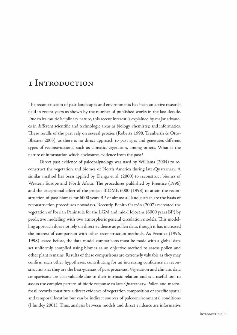
Fig. 1.2 – Earth orbital parameters
Th e pace of climate change is mainly controlled by three or-bital perturbations described
by the Croll-Milankovitch theory. Eccentricity (A) refers
to the changing shape of the Earth’s orbit around the sun from a near circular to an el-
liptic. Th e cycle of this orbital propriety has a period of 400 and 100 ky. Th e axis of rota-tion (B) modifi es its position with amplitude of 2.4º every
41 ky. Th e precession (C) is a characteristic of objects
in rotational movement: the axis has not a fi xed position
and wobbles describing a circular movement in space.
Modulated by eccentricity, this perturbation has a period
of 23 and 19 ky. Data are adapted from Zachos et al.
(2001).
Th e Earth is constantly suff ering from periodical phenomenon that creates a
dynamic climate, by the shifting nature of incident solar energy (Zachos et al. 2001).
Some occur at a human temporal scale and with direct biological consequences as
the daily light cycle or the sequence of seasons caused by rotation and inclination of
Earth axis. Th ese factors have an immediate infl uence in living organisms, easily per-
ceived in annual activity and circadian rhythms.
Several other factors occur at longer scales, contributing to a climatic history
of periodical oscillations. As consequence, life on the planet underwent distribution
changes, extinction and speciation events until achieving its present diversity. Th e
study of the genetic consequences of these events allows the disclosure of the evolu-
tionary process (Hewitt 2004b). Th e climatic history is characterized by colder and
warmer stages, drifting from massive expansion of polar ice-sheet and decrease of
sea level to free polar ice caps and sea level rising. Distinct Earth orbital parameters
described by the Croll-Milankovitch are responsible for the climatic pace: (1) eccen-
tricity refers to the shape of Earth orbit around the Sun, shifting from quasi circular
to elliptic and with a 400 and 100 ky cycle; (2) obliquity of Earth axis in relation to
orbital plan, tilting from 22.1º to 24.5º and responsible for a 41 ky pace; (3) axial
precession or the wobble of axis of rotation every 23 and 19 ky (Hewitt 2000,
1.2 Climatic Oscillations
Introduction |
Zachos et al. 2001). Isolated or combined together, these orbital perturbations shape
the distribution of solar radiation in Earth’s surface. Whereas intensity and season
contrast are balanced by eccentricity and axial precession, the most exposed hemi-
sphere is determined by obliquity. Other intrinsic factors of the Earth had a huge in-
fl uence in the planet’s history and climatic oscillations. Topographic, bathymetric
and atmospheric features, conditioned mainly by plate tectonics, had eff ects at a
million year time scales and increased climate complexity and diversity (Zachos et al.
2001).
Evidence of Milankovitch cycles were found in several reconstructions and it
was observed a prevalence of orbital parameters over each other: 8 My ago the 100
ky the glacial/interglacial cycle was weak whereas in the last 2 My dominated the
climate change (Augustin et al. 2004, Cox & Moore 2005), i.e., during the
Quaternary. Warming and cooling phases do not occurred with stable increments or
declines of temperature. During the last 150 ky, a succession of warm/cold cycles
took place, building a dynamic climate (Alley & Clark 1999, COHMAP 1988,
Folland et al. 2001, Grafenstein et al. 1999, Petit et al. 1999, Zachos et al. 2001).
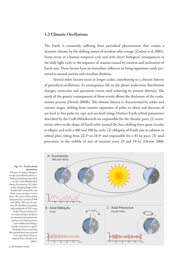
Th e Quaternary (Fig. 1.2), especially the late-Pleistocene and Holocene are charac-
terized by sudden events in the warming phase until present time. Th e Last Glacial
Maximum (LGM) extended from 25 to 18 ky BP followed by warming trend, or the
beginning of deglaciation known as the Bölling-Alleröd event. Th is warming phase
was abruptly discontinued with the Younger Dryas (YD), a cold event about ~12.7
to 11.5 ky BP. When compared to modern climate, the YD is characterized by cold,
dry and windy conditions (Alley & Clark 1999). Th e Holocene is a warming period,
starting at 10 ky BP until present, and at its earliest phase was generally warmer then
the 20th century (Folland et al. 2001). As other periods, it was not free from oscilla-
tions. It had a maximum warming at ~4.5 to 6 ky BP across Europe and a fast cold
event about ~8.2 ky BP (Alley et al. 1997, Folland et al. 2001, Rohling & Palike
2005). Th is latter event had a similar pattern to YD event (Alley & Clark 1999)
with a worldwide decrease of 2ºC of annual mean temperatures (Folland et al. 2001,
Rohling & Palike 2005, Wick & Tinner 1997). Strong climatic oscillations during
the last 20 ky due to orbital perturbations had shaped the distribution of life in
Earth’s surface and left behind clues that can be analysed to reconstruct past
environments.
Fig. 1.2 – Main climatic events during the late-Qua-ternaryTh e late-Quaternary com-prises the end of Pleistocene and the Holocene. Th e fi rst begun at ~150 ky BP with the Last Glacial from ~74 to 14 ky BP and reaching the LGM at ~25 to ~18 ky BP, when the deglaciation have started. Th e Holocene begun at ~10 ky BP until the present. Th e warming of climate is an unstable process: it had pronounced events that oppose to or emphasize the general trend. Th e cold event 1 is the Oldest Dryas (~18 to 14.5 ky BP) that took place at the beginning of deglatiation, which extends until the be-ginning of Holocene at ~10 ky BP. A noticeable warmer event (2), the Böling-Alleröd, occurred from 14.5 to 13 ky BP in Europe, followed by the Younger Dryas (3), a well studied cold event. Th e event 4 happened at 8.2 ky BP and it was a sudden reversal to cold with a brisk appearance. Th e Holocene Maximum Warming (5) or the warmest phase of the Holocene took place from 6 to 4.5 ky BP.

| Introduction
Th e reconstruction of past conditions is based on proxies that refl ect past climate or
vegetation composition. Th ere is an ample variety of data sources and choosing
between them depends on the kind of reconstruction needed. Due to high correla-
tion with temperature, proxies like oxygen or carbon isotopes (δ 18O and δ 13C, re-
spectively) are used since several decades to build climatic reconstructing to obtain
high-resolution data (Zachos et al. 2001) and information about abrupt climate
changes (Crowley & North 1988). Fossil remains of pollen, other vegetation struc-
tures and animals are precise evidence of past biological composition and may also
serve as indirect climate proxies. Th e reconstruction of past vegetation assumes that
there is a plant feedback to climate shifts with immediate results on its distribution
and composition (Hewitt 2004a, Huntley & Webb 1989, Williams et al. 2004), con-
fi guring a dynamic and complex system.
A requisite for paleo-reconstructions is precise dating, which can be obtained
by a careful selection of sample sites and using the most recent dating techniques
(Vandenberghe et al. 1998). Th ere are several dating methods which may be clus-
tered into four major groups: (1) historical, based on known date events and detecta-
ble in data; (2) biological, based on increment quantity related to time as the tree
rings; (3) paleomagnetism with secular variation and (4) radiometric, based on radi-
oactive decay propriety of elements (Roberts 1998). Th e latter are the methods most
used since there is a vast availability of data and results are eff ortless, when compared
to other methods. Th e radiometric most frequently used is the 14C that allows the
datation of organic matter from ages comprehended between 200 and 40 ky, with an
error of 20 - 1.000 years (Roberts 1998). Th is interval includes all Holocene and a
portion of Pleistocene. It is based on the rate of radioactive decay of elements as a
geological clock. Th e half-life is a measure of radioactive decay and in the case of 14C
is 5730±40 years, which is the time its radioactivity decreases by half (Roberts
1998). When the organism dies, their 14C content ceases to be replaced and the
clock begins. Th e major disadvantage of this method is the impossibility to use in
more recent ages due to phenomena with human origin. Th e fossil fuel combustion
since industrial revolution as well more recent nuclear experiments has introduced
on the atmosphere “older” carbon, misleading the dating method to yield farther
dates (Roberts 1998). To increase the precision of this method, Stuiver et al. (1998)
proceed to a calibration with parallel data as tree rings and marine data (Reimer et
al. 2004, Stuiver et al. 1998).
One method for the reconstruction of past landscapes and detect past species’
presence is the analysis of organism’s remains, a process globally known as paleoecol-
1.3 Reconstruction of past landscapes

Introduction |
ogy. Palynology is one of its most important branches and concerns to the study of
fossil pollen that represents a vegetation structure of the study area for a specifi c time
(Roberts 1998). Plant reproduction produces pollen spores and these are preserved
in lake muds, peat bogs and other sediments, allowing posterior analysis of the
remains (Roberts 1998). Th e information extracted from pollen cores has a multi-
variate nature off ering multiple aspects of past environmental conditions, being one
of the major advantages to other physical or chemical proxies (Huntley 2001). Th e
analysis of a pollen site requires a core drilling and posterior analysis in laboratory of
the remainings, often reaching low taxonomic levels as families, sub-families, genuses
or even species (Cox & Moore 2005, Huntley 2001). Th e outputs of this method
include raw pollen counts and a pollen diagram representing percentages of pollen
presence by time or depth, and by taxa. However, it is a time consuming method and
there is a low number of high temporal resolution studies (Huntley 2001), despite
the large amount of paleovegetation data available worldwide since LGM (Prentice
et al. 1998).
Direct evidence from the past vegetation is given by fossil pollen, whereas
other data is obtained indirectly with proxies. However, assumptions have to be
made to achieve a conclusive use of pollen data: the morphology of present plant
pollen and the response range to environmental conditions did not suff ered signifi -
cant changes from past species and there is a dynamic equilibrium of distribution
patterns with climate change until present equilibrium (Huntley 2001). One major
drawback of pollen analysis is the non linear equivalence between pollen abundance
and abundance of mother plants (Odgaard 1999). Nevertheless, it is necessary to
deal with this complexity and biased input because it provides a quantitative evi-
dence that can be subjected to statistical analysis (Williams et al. 1998).
A possible way to use this information is converting pollen percentages to
biomes through plant functional types (Prentice et al. 1996). PFTs are assemblages
of plant taxa that occur in similar environmental conditions, despite its phylogeny
(Prentice et al. 1996, Rusch et al. 2003). Signatures from plant species (e.g. leaf form,
phenology, climatic thresholds and others) are used as functional traits that inhibit
or promote growth under certain conditions, grouping similar taxa together (Grime
et al. 1997, Prentice et al. 1996, Rusch et al. 2003). Th erefore, the usage of PFTs
throughout a time span discloses patterns of fl ora migrations in presence of stressful
conditions (Rusch et al. 2003). Setting up biomes from PFTs is the following step to
produce useful information from pollen percentages. Biomes stress the link between
plant presence and environmental conditions as they are combinations of PFTs. Th e
major advantage of biomes is that they can predict global distributions and may be
compared spatially, temporal and with biomes resulting from other climatic recon-
structions, such as the global circulation models of climate where climatic parameters
are derived from mathematical simulations (Prentice et al. 1996, Williams et al.

| Introduction
1.4 GIS in past vegetation reconstructions
1998). Biomes reconstructions based on paleopalynology are supported by direct ev-
idence of the past, therefore, they may serve as benchmark to other indirect models
(Prentice et al. 1996, Prentice et al. 1998). Successful comparisons between past
biomes and modern pollen data exhibited a congruence between past and present
biomes and detected anthropogenic infl uence in its distribution (Prentice et al.
1996). Biomes also served as benchmarks for other climatic simulations and discrep-
ancies were found due to inaccuracies in climate simulations, in biomes derived by
simulations and in methods for biomization; although the latter was not the major
source of error (Williams et al. 1998). Th e behaviour of both reconstructions (based
in direct and indirect data) was also assessed by others authors ( Jost et al. 2005)
using high resolutions simulations and it was found a general correspondence
between models, with minor temperature discrepancies in Western Europe.
Th e reconstruction of past landscapes may follow several methodological
pathways. Nevertheless, those based in direct past evidence provide accurate dating,
yield good benchmarks to all others studies, and carry important information about
past vegetation processes, especially when studied from a spatial point of view.
Th e number of palynological sites being studied is increasing due to great interest in
past reconstructions. Dealing with a high amount of data from each site and to assess
the larger scale patterns of all analysed sites is arduous and requires a large database
linked to a Geographical Information System (GIS). Th is tool assigns a spatial
context to acquired data, making the visualization and quantitative analysis easier.
Th e need for spatially explicit reconstructions grants the continuous growing of
paleobiogeographical research in the future with the increasing usage of this tool
(Stigall & Lieberman 2006).
Th e most notorious advantage of GIS is the map construction, where is possi-
ble to assemble all data and discern areas of greater or lesser uncertainty in concern
to samples distribution (Prentice et al. 1998). Th e reconstruction of species past dis-
tributions has been an important research fi eld and this tool allows to work with
every scale needed, ranging from local to continental, enhancing the visualization of
species migration patterns with precision (Stigall & Lieberman 2006).
Paleobiogeography expands the normal temporal scale in ecologic studies to geologic
timescale, thus making possible the examination of distribution patterns throughout
time (Rode & Lieberman 2004).
What is the multivariate nature of the palynology data that GIS have to deal
with? Th ese type of data carries evidences from the past revealing several processes
acting simultaneously which shaped the vegetation composition at each site (Huntley

Introduction |
Fig. 1.3 – Biomes recon-structed for present time, 6ky BP and 18 ky BPTh e most widely used method to reconstruct past vegetation is the classifi cation of assemblages in Biomes. Th e BIOME 6000 group has mapped the worldwide distribution of biomes based on the available pollen sites. Data used to produce these maps is freely available to the scientifi c community from the website: http://www.bridge.bris.ac.uk/resources/Databases/BIOMES_data [Prentice et al. (2000), Har-rison et al. (2001), Bigelow et al. (2003), Pickett et al. (2004)].
2001). GIS have a great power to deal with this complex information, as it provides
tools to analyse qualitatively (by discerning patterns) and quantitatively with the use
of traditional and spatial statistics (Stigall & Lieberman 2006). Several past recon-
structions have been made with the aid of GIS. Prentice et al. (1996), in the scope of
BIOME 6000 project, mapped biomes at sampled sites for the LGM and mid-
Holocene (Fig. 1.3). Th is study separated biomes geographically and gave insights of
distribution changes during late-Quaternary. Williams et al. (2004) made an exten-
sive study of biomes in North America, encompassing United States of America and
Canada, with a time lag of 1.000 years between mapped distributions. Paez (2001)
used in Argentina spatial interpolations techniques to improve the mapping features
of modern pollen vegetation. Th ese studies suggested that GIS can produce a large
quantity of results easily interpreted and the increasing processing power along with
the development of new GIS tools are indispensable in past reconstructions.

| Introduction
Th e eff ects of climatic shifts during the late-Quaternary on the distribution of plants
throughout time have been reported at world and continental scales. However, there
is a lack of information for regional scales especially inside refuge areas. Th erefore,
the main purpose of this study is to reconstruct the past vegetation cover in the
Iberian Peninsual and the Balearic Islands. Th is was subdivided in:
1) Reconstruct the distribution of plant genera, PFTs and biomes in the
Iberian Peninsula and the Balearic Islands for late-Quaternary with a 1.000 years
time interval. Past distribution maps are reconstructed with interpolation algorithms
from pollen counts in a GIS environment.
2) Relate the distributions of biomes and climate data. Biomes are linked to
climate oscillations and warmer and colder areas defi ned by biomes are depicted
throughout space and time with support of quantitative analysis with independent
temperature.
3) Identify probable areas for the persistence of plant genera throughout time.
With the results from objectives 1) and 2) it will be analysed the possible migration
routes and delimited the probable refuge areas for tree genera in the Iberian
Peninsula and the Balearic Islands.
Additionally, several tools to automate processes of biomization and creation
of large datasets of distribution maps were produced. Scripts developed in Python
and Visual Basic for Applications programming languages inside a GIS environment
will generate an output with quantitative comparisons between the resulting maps.
Th e application of these scripts are explained in the methods section and presented
in Appendices II to IX.
1. 5 Objectives

Data and Methods |
Data and Methods
2.1 Study Area
Th e study area covers the Iberian Peninsula and the Balearic Islands. Th e Iberian
Peninsula is located in the western-most mainland Europe and includes Portugal
and Spain with an area of ~580.000 km2 (Fig. 2.1). Th e northern and western con-
tinental shelves are bathed by the Atlantic Ocean, whereas at the south and eastern it
is bordered by the Mediterranean Sea. It is isolated from the rest of Europe except
by the Pyrenees mountain chain. Th e Strait of Gibraltar is the most southern part of
the peninsula and separates it from the African continent.
Th e high plateaus prevail in the Iberian Peninsula, divided by the Central
Mountain System, into Northern and Southern Plateaus. Th e plateaus are isolated
from the sea by the Cantabrean Mountains in the north and the Baetic Mountains
in the south. Th e north-eastern area is covered by the Iberian Mountain System,
Fig. 2.1 – Study areaTh e study area comprises the Iberian Peninsula and the Balearic Islands. Th e main topographic futures of this peninsula are the mountain systems with a west-east ori-entation in the north (Can-tabrean mountains), centre (Central Mountains) and south (Baetic Mountains). Th ere are also the Pyreenes and the Iberian Mountains, located in eastern Iberia. Main rivers include the Ebro, Tejo, Douro, Guadalquivir, Guadiana and Minho.

| Data and Methods
2.2 Dataset
parallel to the Ebro River which fl ows to Mediterranean Sea. All remaining main
rivers fl ow to the Atlantic Ocean.
Th e Balearic Islands are an archipelago in the Mediterranean Sea, located at
approximately 200 km from the eastern coast of Iberian Peninsula (Fig. 2.1). It is
composed by four islands: Majorca, Minorca, Ibiza and Formentera with a total area
of 5.000 km2.
Th e Iberian Peninsula is divided in two macrobioclimatic areas: the Temperate
zone mainly in the north and the Mediterranean zone, occupying a large area of the
centre and south of the peninsula (Rivas-Martínez et al. 2004) (Fig. 2.2). Th e latter
is characterized by less then two consecutive arid months during the warmest period
of the year. Th erefore, the average precipitation (in mm) of the two warmest months
in summer is lesser than the double of the average temperature (in ºC) of the same
two months (Rivas-Martínez 2005). Th e Temperate bioclimate expands through
places where there less than (or it is balanced) two or more consecutive arid months
in the summer, i. e., when the average precipitation value (in mm) of the period of
the two warmest months of the summer is higher then the average temperature (in
ºC) of the same period (Rivas-Martínez 2005).
A total of 77 palynological sample sites were analysed (table 2.1). Th is dataset is
composed by 53 digitized sites collected from published pollen diagrams and 24
samples from the European Pollen Database (http://wdc.obs-mip.fr/epd/epd_
Fig. 2.2 – Iberian Peninsula Bioclimatic zones
Th e Iberian Peninsula has a pronounced diff erentiation between bioclimatic zones. In the north dominates the Temperate bioclimate, with
colder temperatures and higher precipitation than the
Mediterranean. Th is biocli-mate occurs mainly in the
south and central peninsula.

Data and Methods |
No. Src. Author Year Latitude Longitude Site name
1 D Desprat, S. 2003 42.2345 -8.7895 Ria de Vigo
2 D Carrión, J. S. 2002 36.9 -2.91667 Sierra de Gádor
3 D Múgica, F. F. 1998 40.8 -3.93 Rascafria (Sierra de Guadarrama)
4 D Santos, L. 2000 42.64 -7.01 Laguna Lucenza (Sierra de Courel)
5 D Santos, L. 2000 42.18 -7.29 Fraga (Sierra de Queixa)
6 D Múgica, F. F. 2001 41.95667 -3.935 Espinosa_Cerrato
7 D Carrión, J. S. 2001 38.8 -2.36667 Villaverde
8 D Goñi, M. F. S. 1999 42.03333 3.033333 Las Pardillas
9 D Leira, M. 2002 42.6 -3.4 Laguna Lucenza
10 D Valero-Garcés, B. 2000 41.50278 -0.73333 Salada Mediana (Ebro Basin)
11 D Sobrino, C. M. 2004 42.11667 -6.71667 Lleguna (Lago de Sanabria)
12 D Sobrino, C. M. 2004 42.13333 -6.7 Laguna de las Sanguijuelas (Lago de Sanabria)
13 D García, M. J. G. 2002 42.02389 -2.75 Hoyos de Iregua (Sierra de Cebollera)
14 D Santos, L. 2003 38.08333 -8.78333 Santo André
15 D Ramil-Rego, P. 1998 42.04 -8.87 Lagoa de Marinho
16 D Ramil-Rego, P. 1998 43.6 -7.8 Mougás
17 D Ramil-Rego, P. 1998 43.5 -7.69 Pena Vella
18 D Ramil-Rego, P. 1998 42.71 -7.21 Chan do Lamoso
19 D Ramil-Rego, P. 1998 41.91 -8.19 Pozo do Carballal
20 D Ramil-Rego, P. 1998 42.77 -3.6 La Piedra
21 D Sobrino, C. M. 2001 42.58333 -7.11667 Laguna de Lucenza
22 D Carrión, J. S. 2002 38.4 -2.5 Siles
23 D Carrión, J. S. 2001 38.06667 -2.7 Cañada de la Cruz
24 D van der Knaap, W.O. 1995 40.34167 -7.57639 Charco da Candieira A
main.html, last accessed in May 2007). Th e sample network covers all Iberian
Peninsula and Balearic Islands but it is not uniformly distributed. Th e south-western
portion of the Iberian Peninsula is less sampled with only 15% of the sampled sites
(Fig. 2.3). Sampled sites do not share the same sampled ages (Fig. 2.4), as a conse-
Fig. 2.3 – Sampled points distributionTh e symbol l represents the digitized dataset, whereas the symbol p represents the da-taset provided by EPD. Th e southwestern area has less coverage, nevertheless there is a reasonable distribution of sampled sites.
Table 2.1 – Dataset originTh e data of sampled sites have two possible origins: they were digitized (D) from published pollen diagrams (53 sites) or they were raw pollen counts from the EPD (24 sites). While the digital raw counts off er more resolu-tion, the digitized data were important to fi ll out the gaps of the sampled network in the study area. (Continues in the next page)

| Data and Methods
No. Src. Author Year Latitude Longitude Site name
25 D van der Knaap, W.O. 1995 40.34167 -7.57639 Charco da CandieiraB
26 D van der Knaap, W.O. 1995 40.34167 -7.57639 Charco da CandieiraC
27 D van der Knaap, W.O. 1995 40.34167 -7.57639 Charco da CandieiraD
28 D van der Knaap, W.O. 1995 40.34167 -7.57639 Charco da CandieiraE
29 D Zapata, M. B. R. 2002 42.02 -3.04 Quintanar de la sierra
30 D Valiño, M. D. 1999 39.07 -3.86 La Cuenca alta
31 D Múgica, F. F. 2001 41.18 -3.11 Turbera de pelagallinas
32 D Sobrino, C. M. 2005 43.53 -7.57 Chan do Lamoso
33 D Sobrino, C. M. 2005 43.55 -7.5 Penido Vello
34 D Sobrino, C. M. 2005 43.07 -3.67 Puerto de los Tornos
35 D Sobrino, C. M. 1997 42.70556 -7.11111 Suárbol
36 D Sobrino, C. M. 1997 42.86389 -6.85278 A Golada
37 D Sobrino, C. M. 1997 42.76806 -6.85 Brañas de Lamela
38 D Sobrino, C. M. 1997 42.70556 -7 Pozo do Carballal
39 D Sobrino, C. M. 1997 42.87778 -6.99722 A Cespedosa
40 D Sobrino, C. M. 1997 42.87778 -7 Porto Ancares
41 D Valiño, M. D. 2002 39.08333 -3.86667 La Mancha plain
42 D Taylor, D. M. 1998 38.82 -2.32 El Jardin
43 D Taylor, D. M. 1998 38.66667 -2.42 Alcaraz
44 D González-Sampériz, P. 2004 42.8 -0.39778 Portalet
45 D van der Knaap, W. O. 1997 40.3375 -7.57972 Charco_da_Candieira
46 D van der Knaap, W. O. 1997 40.36333 -7.64167 Lagoa Comprida 1
47 D van der Knaap, W. O. 1997 40.33917 -7.61111 Charca_dos_Cões
48 D van der Knaap, W. O. 1997 40.33556 -7.605 Lagoa Clareza
49 D Stevenson, A. C. 1985 37.16 -6.84 Laguna de las madres 2
50 D Stevenson, A. C. 1988 37.11667 -6.5 El Acebron (Huelva)
51 D Múgica, F. 2001 41.26667 -3.11667 Pelagallinas
52 D Julià, R. 1998 39.98889 -1.87361 La Cruz
53 D Múgica, F. 2005 41.32003 -4.14697 El Carrizal
54 EPD Burjachs, F. 1994 39.79278 3.119167 Albufera Alcudia (Balearic Islands)
55 EPD Yll, E-I. 1997 39.94056 3.958611 Algendar (Balearic Islands)
56 EPD Mariscal, B. 1993 43.11778 -4.01667 Alsa
57 EPD Pantaleon Cano, J. 1997 37.20833 -1.82361 Antas
58 EPD Penalba, C. 1989 43.25 -1.55 Atxuri01
59 EPD Perez-Obiol, R. 1994 42.13333 2.75 Banyoles
60 EPD Penalba, C. 1989 43.03333 -2.05 Puerto de Belate
61 EPD Yll, E-I. 1997 39.93694 3.965 Cala Galdana (Balearic Islands)
62 EPD Yll, E-I. 1997 39.87056 4.131389 Cala’n Porter (Balearic Islands)
63 EPD Mariscal, B. 1983 43.11667 -4.36417 Cueto de Avellanosa
64 EPD Yll, E-I. 1997 39.875 4.126389 Hort Timoner (Balearic Islands)
65 EPD McKeever, M.H. 1984 43.05 -6.15 Lago de Ajo
66 EPD Allen, J.R.M. 1996 42.21667 -6.76667 Laguna de la Roya
67 EPD Carrion, J.S. 1996 39.1 -0.68333 Navarres (core 1)
68 EPD Carrion, J.S. 1996 39.1 -0.69 Navarres (core 2)
69 EPD Mariscal, B. 1986 43.21556 -4.43611 Pico del Sertal
70 EPD Mariscal, B. 1989 43.12139 -3.70056 Puerto de las Estaces de Trueba
71 EPD Penalba, C. 1989 43.15 -3.43333 Puerto de Los Tornos
72 EPD Penalba, C. 1989 42.03333 -3.01667 Quintanar de la Sierra
73 EPD Pantaleon Cano, J. 1997 36.79444 -2.58889 Roquetas de Mar
74 EPD Penalba, C. 1989 43.05 -2.71667 Saldropo
75 EPD Pantaleon Cano, J. 1997 36.77361 -2.60139 San Rafael
76 EPD Hannon, G.E. 1985 42.1 -6.73333 Sanabria Marsh
77 EPD Yll, E-I. 1997 39.92472 4.027222 Sou Bou (Balearic Islands)
Table 2.1 – Dataset originContinued.

Data and Methods |
0
10
20
30
40
50
60
70
0 1 2 3 4 5 6 7 8 9 10 11 12 13 14 15 16 17 18 19 20 21
Sampled Ages (ky BP)
Nu
mb
er o
f sa
mp
led
sit
esquence of diff erences in the methodology applied to palynological analysis. Th ere are
sampled sites with higher temporal resolution, such as the Banyoles site (no. 59 in
table 2.1) that extends the palynological analysis for 30 ky, ranging from 6 to 35 ky
BP, covering almost all studied timescale. Th ere is a peak at 3 ky BP with 61 sampled
sites and the lower value is at 15 ky BP with 15 sampled sites. Although there is an
evident reduction of the available data towards the past, the study area is reasonably
covered with sampled sites available from 15 to 1 ky BP (Fig. 2.5). To accept as a
valid age to reconstruct past distributions, it was chosen a threshold of 19 sample
sites available as the minimum. Th is threshold is a trade-off between the number of
palynological sites and their geographic distribution with statistical signifi cance for
the interpolation algorithm (see below, 2.4). Th e interval to collect pollen percentag-
es was 1.000 years, since 15.000 until 1.000 BP.
Th e EPD supports a free database with a friendly user interface where data
can be obtained as raw pollen counts. All pertinent data was extracted with the re-
spective 14C age samples. Raw counts were converted to pollen percentages and data
of needed ages were obtained by linear interpolation of calibrated 14C controls
(Elenga et al. 2000, Williams et al. 2004). Digitized pollen diagrams do not provide
the same accuracy as digital data as they present data in pollen percentages instead
of raw pollen counts and taxa with lower presence are often misjudge. Nevertheless,
digitized data was required to extend the sample network. Control ages in 14C dates
obtained at diff erent depths of each sampled point are shown in the published pollen
data diagrams. Th ey were calibrated to real BP dates and the percentages of pollen
of sampling ages were extracted directly from the diagram.
Th e calibration of 14C dates to real calendar was executed with the OxCal 4ß
software (Ramsey 1995, 2001). Th is process insures that all ages have passed
through the same calibration process, representing with higher accuracy the pretend-
ed age without discrepancies between diff erent methods. INTCAL04 (Reimer et al.
2004) was the chosen curve in the software to interpolate real dates from the uncali-
brated 14C samples.
Fig. 2.4 – Number of sam-pled sites by sampled ageTh e number of available sites by age is not constant. It increases until the maximum at 3 ky BP with 61 sampled points and decreases until 15 ky BP with a minimum ac-cepted of 19 sampled points. Th is value excludes the present and all years before 15 ky BP.

| Data and Methods
Th e biomization method was described in detail by Prentice et al. (1996) and
Prentice & Webb (1998). In general, this method attributes several taxa to PFTs and
afterwards it classifi es these PFTs into biomes at each sampled point. An affi nity
index is calculated and it weights the biome at each point. Although all biomes have
an affi nity to a sample point, the one with the maximum value is assumed to prevail
(Prentice et al. 1996).
Th e PFTs are groups of taxa assigned by bioclimatic affi nity and plants phe-
nology traits and therefore this classifi cation retains much of bioclimatic information
(Prentice et al. 1996, Prentice et al. 1998). Despite the unavailability of standard
methods to classify PFTs and biomes (Prentice et al. 1998), the comparison between
results is needed. Th erefore, the current study adopted a nearly universal classifi ca-
tion scheme for Quarternary biomes already used by other researchers (Elenga et al.
Fig. 2.5 – Location of sam-pled sites between 15 and
1 ky BP in Iberian Penisula and the Balearic Islands
Th e time resolution diff ers between sample points. Some extended throughout all late-Quaternary while others did
not. Th is confi gures a slightly diff erent network of sampled
point for each age, but the coverage of the study area
remains the same.
2.3 Biomization procedure

Data and Methods |
Code PFT Pollen taxa aa arctic/alpine dwarf shrub Alnus, Betula, Empetrum, Dryas, Rhododendron, Salix, Saxifraga,
Vaccinium bec boreal evergreen conifer Abies, Picea bs boreal summergreen Betula, Alnus, Salix ctc cool-temperate conifer Abies ctc intermediate-temperate conifer Cedrus df desert forb/shrub Ephedra ec eurythermic conifer Juniperus, Pinus subgen. Diploxylon g grass Poaceae
h heath Ericaceae, Calluna sf steppe forb/shrub Artemisia, Apiaceae, Armeria, Asteraceae, Brassicaceae,
Campanulaceae, Caryophyllaceae, Centaurea, Chenopodia-ceae, Dipsacaceae, Ephedra fragilis, Fabaceae, Helianthemum, Hippophae, Plantago, Polygonum, Rosaceae, Rubiaceae, Rumex, Sanguisorba, Th alictrum
ts temperate summergreen Alnus, Fraxinus excelsior, Populus, Quercus (deciduous), Salix ts cool-temperate summergreen Carpinus, Corylus, Fagus, Tilia, Ulmus ts warm-temperate summergreen Ostrya wte warm-temperate broadleaved evergreen Quercus (evergreen) wte cool-temperate broadleaved evergreen Buxus, Hedera, Ilex wte warm-temperate sclerophyll shrub Olea, Phillyrea, Pistacea
(1)
Table 2.2 – Taxa by PFTTh e assignment of pollen taxa to plant functional types (PFTs) used as an intermedi-ate process to produce the Biomes.
2000, Peyron et al. 1998, Prentice et al. 1996). Th ese biomes were used in several re-
constructions and using them in the present study allows a comparison with other
works. A matrix of taxa vs. PFTs (table 2.2) is built with pollen percentages and
crossed with a matrix of PFTs vs. Biomes (table 2.3) to yield a fi nal matrix with
biomes and the allowed taxa with binary values of presence/absence. Th e affi nity
index is given by equation (1):
where Aik is the affi nity index of a sample point k for the biome i. ∑j is the sum
of all taxa and δij is the presence/absence value of taxon j in biome i. Th e pollen per-
centage is represented by p subtracted by a threshold pollen percentage (θ). For the
latter it was adopted the universal threshold of 0.5% (Prentice et al. 1996, Prentice
et al. 1998). Th e incidence of misassignment among relatively species-poor assem-
blages is reduced, although there may be a nearly identical affi nity for several biomes
(Prentice et al. 1998). Th is occurs because single pollen from diff erent taxa could
have a major eff ect in biome affi nity: a point site with two taxa with 10% yields half
affi nity score to a biome than eight taxa with 2.5% (Prentice et al. 1998). Th ese low
pollen counts may derive from long-distance transport during polinization or sample
contamination. Th is 0.5% threshold does not assure that the long-distance transport
is eliminated, because some taxa can produce large amount of pollen that could
result in high percentages at other local. However, setting a higher value could elimi-
nate positive information from other taxa with low pollen expression. Th erefore, a
low but non-zero value is acceptable (Prentice et al. 1998).

| Data and Methods
Code Biome Plant functional types
CLDE cold deciduous forest bs, h TAIG taiga bec, bs, ec, h CLMX cold mixed forest bs, ctc, ctc, ec, h, ts1 COCO cool conifer forest bec, bs, ctc, ec, h, ts1 TEDE temperate deciduous forest bs, ctc, ctc, ec, h, ts, ts1, ts, wte1 COMX cool mixed forest bec, bs, ctc, ec, h, ts, ts WAMX broadleaved evergreen/warm mixed forest ec, h, ts, ts, ts, wte, wte1 TUND tundra aa, g, h XERO xerophytic woods/scrub ec, wte, wte2 STEP steppe g, sf DESE desert df
2.4 Data visualization and analysis
Th e genera and PFTs were mapped by interpolating individual or average percentag-
es, respectively, at sample points by ordinary kriging technique at each sample age.
Th is method estimates weighted linear combinations of data and diff ers from other
interpolations methods by attempting to maintain a zero mean residual error, i. e.,
unbiased results, and minimizing the variance of the errors (Isaaks & Srivastava
1989). Th is is achieved by creating a model of the data to calculate the bias and error
variance, otherwise they are unattainable (Isaaks & Srivastava 1989). Kriging
method is also able to incorporate in the model the eff ects of spatial autocorrelation,
that is intrinsic to biological data (Edwards & Fortin 2001).
Maps obtained by interpolations techniques are equivalent to isopol maps
(Bernabo & Webb 1977, Williams et al. 2004) and it is assumed that pollen percent-
ages refl ect the plant densities at sampled age (Bradshaw & III 1985, Williams et al.
2004). In this study, pollen percentages values were divided in four classes through a
geometric interval classifi cation scheme. Th is process algorithm generates class
breaks based on class intervals with geometrical series. Th e inverse of geometric co-
effi cient, or the diff erence between the distances of two classes, can change only once
to ensure that each class range has approximately the same number of values, thus
the change between intervals is consistent (ESRI 2006). Th is yields maps with dis-
tinguishable patterns of distribution despite the variation in pollen percentages pe-
culiar to each genus or PFT.
Th e biome maps are representations of maximum affi nities of the interpolated
affi nity surfaces. To produce these surfaces, affi nity for every biome was interpolated
by kriging technique from each sample point. Th e fi nal outcome is a map of biomes
in which each cell represents the biome with the maximum affi nity in the interpolat-
ed surface. Although there are procedures to resolve tied biome affi nities by estab-
lishing a priority order of biomes, this study opted to represent areas of biomes co-
Table 2.3 – PFT by BiomePlant functional types used
to generate affi nity scores to each Biome. Th e PFTs are
abbreviated with the scheme shown in table 2.2.
Data and Methods |
dominance. Th e core areas for the presence of genera was calculated by averaging all
distribution maps for the time span analysed. Th e resulting map provides the loca-
tion of the areas where each genus persisted through the late-Quaternary.
In order to reduce the eff ort of producing a large number of maps, this process
was automated with several scripts. Th ese scripts were developed in Python free pro-
gramming language (http://www.python.org) and implemented as toolboxes in
ArcGIS 9.2. Th ese include toolboxes for create all affi nity surfaces for every biome
using a single interpolation model confi gured in GeoStatistical Analyst Extension
(appendix II), a builder of classifi cation biome surfaces (appendix III) and analyst of
geographic correlations between rasters (appendix IV). Th e remaining scripts made
a routine task of smoothing all available rasters fi les (appendix V), automated the
conversion between raster fi le types (appendix VI) and the extraction of masked
areas from the original rasters (appendix VII). Th e capability to use ArcGIS pro-
gramming objects inside the software was also employed to develop two automating
scripts in Visual Basic for Applications language. Th ese two scripts were an aid to set
up identical classifi cations and graphical displays to all ages for each distribution (ap-
pendix VIII) and export to images with a defi ned size and resolution (appendix IX).
All raster maps were processed with a 0.045 degree resolution (~5 Km) and
the coordinate system used was the geographic WGS84. All genus and PFTs distri-
bution maps as well the interpolated affi nity surfaces were smoothed by an 8 cell
square moving window that collects the surrounding average to each pixel. Th is
process assured that the spatial autocorrelation of data is not represented as sharp
transitions, hence reducing some artefacts of the interpolation method, and also pro-
vides an enhancement of visualization. When pollen percentages data was missing it
was not possible to reconstruct a potential distribution map, which was left blank.
Th is occurred only at farther ages with single genus distributions, which are the most
sensible due to lack of other taxa to compensate the distribution as it happens in
PFTs assemblages or biomes.
Th e quantitative analyses were geographic correlations between raster pixels.
To correlate distributions of pollen percentages by Pearson correlation, it was used
the average presence maps from each mapped taxa and PFT. Th ese core presence
sites throughout time were compared to achieve a correlation value of its geographic
distribution. Th e biomes areas for each year were compared to the average value of
oxygen isotope for the correspondent time interval and extracted the linear trend.
Th is provides a quantitative relationship between temperature sensitive biomes and
the independent temperature proxy to assess the co-evolution of both. Th e evolving
biomes areas were also correlated to the evolution of the temperature proxy to quan-
tify a possible positive or negative correlation.

| Data and Methods

Results |
ResultsTh e pattern of vegetation distribution in the past is considerably diff erent from the
present, notwithstanding the persistence of a stable core of each genus, PFTs or
biome throughout time in specifi c areas (Fig. 3.1). For genus like Alnus, Betula,
Castanea, Quercus deciduous and, to a lesser extent, Fagus the stable core is located in
north and west of Iberian Peninsula (Fig. 3.1). Th e southern and eastern area of the
peninsula holds the distribution of Olea, Pistacia and Quercus evergreen throughout
the late-Quaternary (Fig. 3.1). Th is duality of the global pattern of distribution is
also detectable in the mapped PFTs (Fig. 3.2). Th e boreal summergreen (bf) and the
temperate summergreen (ts) PFTs follow a north-western gradient, contrasting to
the south-eastern distribution of the cool-temperate broadleaved evergreen (wte)
and steppe forb / shrub (sf) assemblages.
Th e biomes present the same pattern of distribution (Fig. 3.2). Th e
maximum affi nity scores of Broadleaved evergreen / Warm mixed forest and
Xerophytic woods/scrub biomes occurs at south portion of the Iberian Peninsula.
On the other hand, the Cool mixed forest occurs mainly in the north and the
Temperate deciduous forest extends for a large area of the Iberian Peninsula, with a
similar pattern to the north-western distribution of several genera and PFTs. Th e
Tundra biome is not present constantly throughout the studied time interval and
appears mainly in the extreme areas of western and eastern Iberia. Th e distribution
of interpolated affi nity surfaces for each biome reveals also this persistent pattern of
distribution (Fig. 3.3). Th e southern distribution pattern exhibited in some genera,
PFTs and biomes often extends to the Balearic Islands.
3.1 Distribution of plant genera
Th ere is a marked diff erence between the eight mapped plant genus distribution,
with some showing a general northern distribution and others occurring in the
southern part of Iberia (Fig. 3.1). Th is diff erence is supported by a geographic corre-
lation value of the average distribution for the studied time-scale (table 3.1). Alnus,

| Results
15 ky BP 14 ky BP 13 ky BP 12 ky BP
Alnus (%)
Quercus (evergreen) (%)
Quercus (deciduous) (%)
Pistacea (%)
Olea (%)
Fagus (%)
Castanea (%)
Betula (%)
0.00 - 0.59 0.59 - 1.48 1.48 - 3.52 3.52 - 100
0.00 - 3.42 3.42 - 3.97 3.97 - 7.12 7.12 - 100
0.0000 - 0.0793 0.0793 - 0.0812 0.081 - 0.1605 0.1605 - 100
0.00 - 0.09 0.09 - 0.45 0.45 - 1.99 1.99 - 100
0.00 - 0.45 0.45 - 0.47 0.47 - 0.89 0.89 - 100
0.00 - 0.08 0.08 - 0.29 0.29 - 0.78 0.78 - 100
0.00 - 8.65 8.65 - 10.84 10.84 - 18.14 18.14 - 100
0.00 - 2.38 2.38 - 4.53 4.53 - 6.95 6.95 - 100
Fig 3.1 – Reconstruction of Genera distribution in Iberian Peninsula and Balearic Islands between 15 and 1 ky BPTh e distribution of Alnus, Betula, Castanea, Fagus, Olea, Pistacia, deciduous and evergreen Quercus was achieved by direct interpolation of pollen percentages between 15 and 1 ky BP. Th ese maps can not be compared between taxa as the production

Results |
11 ky BP 10 ky BP 9 ky BP 8 ky BP
Alnus (%)
Quercus (evergreen) (%)
Quercus (deciduous) (%)
Pistacea (%)
Olea (%)
Fagus (%)
Castanea (%)
Betula (%)
0.00 - 0.59 0.59 - 1.48 1.48 - 3.52 3.52 - 100
0.00 - 3.42 3.42 - 3.97 3.97 - 7.12 7.12 - 100
0.0000 - 0.0793 0.0793 - 0.0812 0.081 - 0.1605 0.1605 - 100
0.00 - 0.09 0.09 - 0.45 0.45 - 1.99 1.99 - 100
0.00 - 0.45 0.45 - 0.47 0.47 - 0.89 0.89 - 100
0.00 - 0.08 0.08 - 0.29 0.29 - 0.78 0.78 - 100
0.00 - 8.65 8.65 - 10.84 10.84 - 18.14 18.14 - 100
0.00 - 2.38 2.38 - 4.53 4.53 - 6.95 6.95 - 100
of pollen diff ers. Nevertheless, they may be analysed through time inside each taxa to achieve the maximum and minimum presence and the distributional shifts. Th e white maps indicate absence of points to model the distributions. Distributions at time 0 of Alnus, Betula, Fagus, deciduous and evergreen Quercus were adapted from Tenorio et al. (2001) and of Castanea, Olea

| Results
Fig. 3.1 - Continued.
7 ky BP 6 ky BP 5 ky BP 4 ky BP
Alnus (%)
Quercus (evergreen) (%)
Quercus (deciduous) (%)
Pistacea (%)
Olea (%)
Fagus (%)
Castanea (%)
Betula (%)
0.00 - 0.59 0.59 - 1.48 1.48 - 3.52 3.52 - 100
0.00 - 3.42 3.42 - 3.97 3.97 - 7.12 7.12 - 100
0.0000 - 0.0793 0.0793 - 0.0812 0.081 - 0.1605 0.1605 - 100
0.00 - 0.09 0.09 - 0.45 0.45 - 1.99 1.99 - 100
0.00 - 0.45 0.45 - 0.47 0.47 - 0.89 0.89 - 100
0.00 - 0.08 0.08 - 0.29 0.29 - 0.78 0.78 - 100
0.00 - 8.65 8.65 - 10.84 10.84 - 18.14 18.14 - 100
0.00 - 2.38 2.38 - 4.53 4.53 - 6.95 6.95 - 100
and Pistacia from Inventário Florestal Nacional (http://www.dgrf.min-agricultura.pt/ifn/mapas.htm) and Proyecto Anthos (http://www.anthos.es/intro_v2.html)

Results |
3 ky BP 2 ky BP 1 ky BP 0
Alnus (%)
Quercus (evergreen) (%)
Quercus (deciduous) (%)
Pistacia (%)
Olea (%)
Fagus (%)
Castanea (%)
Betula (%)
0.00 - 0.59 0.59 - 1.48 1.48 - 3.52 3.52 - 100
0.00 - 3.42 3.42 - 3.97 3.97 - 7.12 7.12 - 100
0.0000 - 0.0793 0.0793 - 0.0812 0.081 - 0.1605 0.1605 - 100
0.00 - 0.09 0.09 - 0.45 0.45 - 1.99 1.99 - 100
0.00 - 0.45 0.45 - 0.47 0.47 - 0.89 0.89 - 100
0.00 - 0.08 0.08 - 0.29 0.29 - 0.78 0.78 - 100
0.00 - 8.65 8.65 - 10.84 10.84 - 18.14 18.14 - 100
0.00 - 2.38 2.38 - 4.53 4.53 - 6.95 6.95 - 100

| Results
Betula, Castanea and deciduous Quercus have a markedly north and western distribu-
tion and maintain high negative correlation with Olea, Pistacia and evergreen Quercus which are distributed in the south. Fagus distribution is not related to other genera,
therefore low correlation levels explain the distinct north-eastern core throughout
time.
Alnus species found in palynological analysis had it fi rst strong appearance in
the north of the Iberian Peninsula at 14 ky BP. Its distribution extended to south-
west, reaching southern areas of the peninsula, in the following 1 ky, achieving high
values of pollen percentages, never reaching the Balearic Islands. Th e presence of this
genus decreased during 12 ky BP before a new extension of its distribution area from
the western Iberia. Th is expansion reaches the Atlantic zone and reasonably main-
tained its distribution until present time, with a core of high pollen percentage values
in the northwest. Th is genus has a strong geographic correlation with Quercus decid-
uous and Betula (Table 3.1). A strong correlation with Quercus evergreen and
Pistacia is found, although negative for both genera.
Betula species preserved a high pollen production throughout time, with
highest values in the half nortwestern part of the Iberian Peninsula. However, it is
noticeable the expansion of the core in the north from 15 to 12 ky BP and its slow
retraction from 10 to 1 ky BP. Th ere is some evidence of this genus presence at 13
and 12 ky BP in the Balearic Islands. An evident negative correlation with Pistacia
genus reveals the diff erent geographic distribution shape.
Th e evolution of Castanea is peculiar when comparing to the other distribu-
tion maps. It has a northern presence and rarely expands further from the nucleus
with high values of pollen percentages. It is near absent from 10 to 6 ky BP but has a
noteworthy recover until 2 ky BP. Its presence in the Balearic Islands was never de-
picted. It shows a robust correlation of the average presence with deciduous Quercus. Decidous Quercus is near absent from Iberian Peninsula from 15 to 13 ky BP,
when it is found a distribution at the western most area of the peninsula. It suff ered
a retraction at 12 ky BP, with the persistence of a nucleus in the northwest. Th is core
expanded in direction of the southeast, however with low expression further than
half of the peninsula. From 10 to 4 ky BP it shows a second nucleus at the north-
eastern portion of the peninsula. Th e dispersion of these genuses never arrives to the
Balearic Islands. Its distribution correlates positively with Alnus and Castanea and it
is the genus that achieves higher values of pollen percentages.
Olea has a markedly south and east distribution. Its pollen percentages values
decreases until 12 ky BP without loosing a core in the extreme south. From 11 to 6
ky BP, its distribution is unstable, with contraction and expansion phases. At 5 ky
BP it has an energetic expansion, reaching almost all area of the peninsula with high
values of pollen percentages. Th e presence of Olea in the Balearic Islands is consist-
ent throughout time, only with low pollen values from 13 to 11 ky BP. Although all

Results |
Alnus Betula Castanea Fagus Olea Pistacea Quercus (deciduous)
Quercus (evergreen)
Alnus 1.00
Betula 0.87* 1.00
Castanea 0.76* 0.66 1.00
Fagus 0.33 0.25 -0.04 1.00
Olea -0.73 -0.82* -0.55 -0.38 1.00
Pistacea -0.86* -0.91* -0.61 -0.49 0.79* 1.00
Quercus (deciduous)
0.90* 0.85* 0.90* 0.13 -0.71 -0.83* 1.00
Quercus (evergreen)
-0.86* -0.69 -0.59 -0.50 0.50 0.81* -0.78* 1.00
Table 3.1 – Pearson’s coeffi ciente of correlations between mapped taxaTh e correlations are made between raster cells of the average distribution through time of each pair of taxa. Th is correlation has a geographic meaning: positive values indi-cate persistence of taxa in the same location, and negative values persistence at diff erent locations. Signifi cant cor-relations (r>0.750) marked with *.
correlations with other species are distant from zero, the highest correlation is with
Betula.
It was not possible to produce distribution maps for genus Pistacia for the far-
thest age. Although the remaining distribution points to a south nucleus, at 13 ky
BP it weakly occupied a western area, without visible expression in the east. Th e ages
of 13 ky BP, 10 ky BP and 1 ky BP had lower values of pollen percentages. From 7
to 2 ky BP it had a constant distribution, with a main area in the south, and expand-
ing to cover most of Iberian Penisula. In the Balearic Islands, Pistacia was present
throughout time with the exception of a lower presence period from 13 to 10 ky BP.
Th is genus presents a very strong negative correlation with Betula.
Th e evergreen Quercus genus has a low expression during the farthest years,
from 15 to 11 ky BP, with presence restricted to the south of the Iberian peninsula.
Th is low expression reached its extreme at 10 ky BP, when its presence is indistin-
guishable. From then onwards, its presence is constant with a nucleus of high pollen
percentage values moving slightly to east. At 3 ky BP is found a weak presence in the
extreme northwest. In the Balearic Islands, evergreen Quercus presence is very low
until 6 ky BP, when it increases. Th e correlation values with other genera are higher
or equal to 0.50 (in their symmetric positive values, if negative), being the highest
with Pistacia.
Th e genus Fagus has a general low pollen percentage values and interpolation
maps for older ages (between 15 and 11 ky BP) were unachievable. From 10 to 1 ky
BP it has a conspicuous expansion from its northern presence. Th is genus presents
the most diff erent pattern of distribution through time when compared to all other
genus. It has a north core of high pollen percentages, slight shifted to east. Genus
Fagus had throughout time a indistinguishable presence in the Balearic Islands. Th is
genus has a near zero correlation values with all other genus, with the highest value
with Quercus evergreen.

| Results
A
B
15 ky BP 14 ky BP 13 ky BP 12 ky BP
bs (%)
ts (%)
wte2 (%)
sf (%)
1
0
-1
-2
-3
-2
-4
-6
0
2
100
80
60
40
20
016 ky BP 15 ky BP 14 ky BP 13 ky BP 12 ky BP
0.00 - 2.39 2.39 - 3.29 3.29 - 5.49 5.49 - 100
0.00 - 2.87 2.87 - 3.51 3.51 - 5.89 5.89 - 100
0.00 - 0.32 0.32 - 0.35 0.35 - 0.64 0.64 - 100
0.00- 1.22 1.22 - 1.52 1.52 - 2.16 2.16 - 100
% b
iom
e ar
eao
xyge
ne
iso
top
ean
om
aly
A
B
biomes clmx comx tede tund wamx
Fig 3.2 – Reconstruction of PFTs and Biomes distribution in Iberian Peninsula and Balearic Islands from 15 to 1 ky BPTh e distribution of four PFTs and biomes were reconstructed from 15 to 1 ky BP. Th e chosen PFTs were bs and ts colder as-semblages and the warmer wte and sf and their distribution was achieved by the interpolation of average pollen percentage of member taxa. Th e actual distribution was not possible to achieve due to low number of sampled sites of paleopollen. Th e Biomes maps were accomplished by fi nding the biome that achieve the maximum value of the interpolated affi nity scores by raster cell. Th e combined biomes are tied affi nity scores between two biomes. Each colour represents a biome or a co-domi-nance of two biomes (described in the upper legend). Th e biome map for time 0 was adapted from Prentice (1996). Distribu-tions at time 0 of PFTs bs and ts were adapted from Tenorio et al. (2001) and wte from Proyecto Anthos (http://www.anthos.es/intro_v2.html). Th e PFT sf, at time 0, is distrubted throughout all the Iberian Peninsula. Graphic A depicts the anomalies of temperature related to last 1000 yeast average throughout time. Blue line represents the GISP2 oxygen isotope record anomaly (Grootes et al. 1997, 1993, Meese et al. 1994, Steig et al. 1994, Stuiver et al. 1995), whereas the red line is temperature anomaly adapted from Heiri (2003). Graphic B depicts the shifts in area of each biome throughout time.

Results |
0.00- 1.22 1.22 - 1.52 1.52 - 2.16 2.16 - 100
11 ky BP 10 ky BP 9 ky BP 8 ky BP
bs (%)
ts (%)
wte2 (%)
sf (%)
1
0
-1
-2
-3
-2
-4
-6
0
2
100
80
60
40
20
012 ky BP 11 ky BP 10 ky BP 9 ky BP 8 ky BP
0.00 - 2.39 2.39 - 3.29 3.29 - 5.49 5.49 - 100
0.00 - 2.87 2.87 - 3.51 3.51 - 5.89 5.89 - 100
0.00 - 0.32 0.32 - 0.35 0.35 - 0.64 0.64 - 100
biomes dese stepxero comx + tedeclmx + tund
Tem
per
atu
re a
no
mal
y

| Results
Fig 3.2Continued.
0.00- 1.22 1.22 - 1.52 1.52 - 2.16 2.16 - 100
7 ky BP 6 ky BP 5 ky BP 4 ky BP
bs (%)
ts (%)
wte2 (%)
sf (%)
biomes clmx comx tede tund wamx
1
0
-1
-2
-3
-2
-4
-6
0
2
100
80
60
40
20
08 ky BP 7 ky BP 6ky BP 5 ky BP 4 ky BP
0.00 - 2.39 2.39 - 3.29 3.29 - 5.49 5.49 - 100
0.00 - 2.87 2.87 - 3.51 3.51 - 5.89 5.89 - 100
0.00 - 0.32 0.32 - 0.35 0.35 - 0.64 0.64 - 100
% b
iom
e ar
eao
xyge
ne
iso
top
ean
om
aly
A
B

Results |
0.00- 1.22 1.22 - 1.52 1.52 - 2.16 2.16 - 100
3 ky BP 2 ky BP 1 ky BP 0
bs (%)
ts (%)
wte2 (%)
sf (%)
biomes dese stepxero comx + tedeclmx + tund
1
0
-1
-2
-3
-2
-4
-6
0
2
100
80
60
40
20
04 ky BP 3 ky BP 2 ky BP 1 ky BP 0
0.00 - 2.39 2.39 - 3.29 3.29 - 5.49 5.49 - 100
0.00 - 2.87 2.87 - 3.51 3.51 - 5.89 5.89 - 100
0.00 - 0.32 0.32 - 0.35 0.35 - 0.64 0.64 - 100
Tem
per
atu
re a
no
mal
y

| Results
It was mapped the past distribution of four PFTs (Fig. 3.2). Th ese plant associations
have diff erent climatic preferences which are revealed by the shifting distribution
patterns throughout time. Th e correlations values among PFTs are indicative of geo-
graphic position of the core throughout time. Th e overall cline of distribution is
similar to genera distribution: a northwest to southeast gradient or reverse, depend-
ing on plant association characteristics.
Th e PFT bs exhibits a northern distribution during the end of the Pleistocene.
At 14 ky BP the core strengthens and expands towards the south and east with
strong presence in the west and the northeast from 13 to 10 ky BP. From 10 to 3 ky
BP, this assemblage has a solid presence in the north and in the western portion of
Iberian Peninsula. At 1 ky BP there are no evidences of intense presence in the
eastern half of the peninsula. Although there are no strong correlations among PFTs,
functional type bs shows a trend for a negative geographic correlation with PFT sf
(Table 3.2). Th is PFT presence in the Balearic Island is just noticeable from 13 to 12
ky BP.
During older ages, evidence of PFT ts was absent from Iberian Peninsula. It
emerged in the western area at 13 ky BP and retracted at 12 ky BP. Its presence was
constant in the west and north of the Iberian Peninsula, expanding into almost all
areas. Th e easternmost area was never permanently occupied, except at 6 and 3 ky
BP. During the latter period, the PFT distribution assumes two cores: one in the
northwest and other in the southeast. Th is south eastern core extends to the Balearic
Islands and it’s the exclusive presence of this PFT in the archipelago. Th e average ts
distribution presents a positive correlation with bs and a negative with sf and wte.
Th e PFT sf dwelt in all area of Iberian Peninsula through 15 to 12 ky BP,
with a retraction in the westernmost area. Th e distribution of pollen percentages at
11 ky BP suff ered its largest contraction and it was confi ned to the south of Iberia,
disappearing also from the Balearic Islands, where this PFT presence was constant
throughout time. From then onwards, it expanded and covered the southern and
eastern half with a notable exception at 7 ky BP, when it had a decrease of pollen
percentage.
bs ts sf wte
bs 1
ts 0.67 1
sf -0.66 -0.58 1
wte -0.73 -0.44 0.46 1
Table 3.2 – Pearson’s cor-relation coeffi cient between
mapped PFTsTh e correlations are made between raster cells of the
average distribution through time of each pair of PFT.
Th e persistence of the pair of PFT throughout time in the same area are depicted by positive values, whereas the negative values indicate
that they do not occur in the same place.
3.2 Distribution of Plant Functional Types
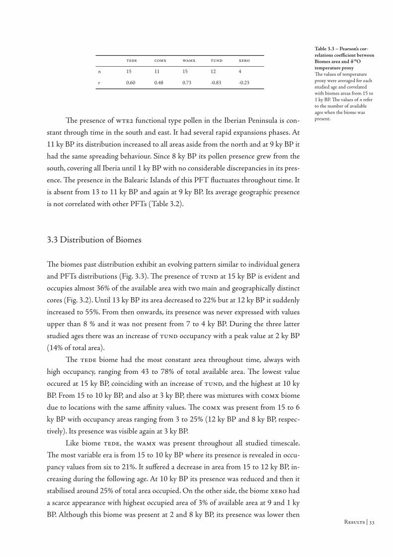
Results |
3.3 Distribution of Biomes
Th e biomes past distribution exhibit an evolving pattern similar to individual genera
and PFTs distributions (Fig. 3.3). Th e presence of tund at 15 ky BP is evident and
occupies almost 36% of the available area with two main and geographically distinct
cores (Fig. 3.2). Until 13 ky BP its area decreased to 22% but at 12 ky BP it suddenly
increased to 55%. From then onwards, its presence was never expressed with values
upper than 8 % and it was not present from 7 to 4 ky BP. During the three latter
studied ages there was an increase of tund occupancy with a peak value at 2 ky BP
(14% of total area).
Th e tede biome had the most constant area throughout time, always with
high occupancy, ranging from 43 to 78% of total available area. Th e lowest value
occured at 15 ky BP, coinciding with an increase of tund, and the highest at 10 ky
BP. From 15 to 10 ky BP, and also at 3 ky BP, there was mixtures with comx biome
due to locations with the same affi nity values. Th e comx was present from 15 to 6
ky BP with occupancy areas ranging from 3 to 25% (12 ky BP and 8 ky BP, respec-
tively). Its presence was visible again at 3 ky BP.
Like biome tede, the wamx was present throughout all studied timescale.
Th e most variable era is from 15 to 10 ky BP where its presence is revealed in occu-
pancy values from six to 21%. It suff ered a decrease in area from 15 to 12 ky BP, in-
creasing during the following age. At 10 ky BP its presence was reduced and then it
stabilised around 25% of total area occupied. On the other side, the biome xero had
a scarce appearance with highest occupied area of 3% of available area at 9 and 1 ky
BP. Although this biome was present at 2 and 8 ky BP, its presence was lower then
tede comx wamx tund xero
n 15 11 15 12 4
r 0.60 0.48 0.73 -0.83 -0.23
Table 3.3 – Pearson’s cor-relations coeffi cient between Biomes area and δ18O temperature proxyTh e values of temperature proxy were averaged for each studied age and correlated with biomes areas from 15 to 1 ky BP. Th e values of n refer to the number of available ages when the biome was present. Th e presence of wte functional type pollen in the Iberian Peninsula is con-
stant through time in the south and east. It had several rapid expansions phases. At
11 ky BP its distribution increased to all areas aside from the north and at 9 ky BP it
had the same spreading behaviour. Since 8 ky BP its pollen presence grew from the
south, covering all Iberia until 1 ky BP with no considerable discrepancies in its pres-
ence. Th e presence in the Balearic Islands of this PFT fl uctuates throughout time. It
is absent from 13 to 11 ky BP and again at 9 ky BP. Its average geographic presence
is not correlated with other PFTs (Table 3.2).

| Results
15 ky BP 14 ky BP 13 ky BP 12 ky BP
clde
clmx
coco
comx
0.26 - 5.07 5.07 - 7.88 7.88 - 9.51 9.51 - 12.32
1.96 - 6.87 6.87 - 9.26 9.26 - 11.65 11.65 - 16.56
1.96 - 6.87 6.87 - 9.26 9.26 - 11.65 11.65 - 16.56
2.98- 10.45 10.45 - 13.31 13.31 - 16.17 16.17 - 23.64
11 ky BP 10 ky BP 9 ky BP 8 ky BP
dese 0 - 0.001 0.001 - 0.045 0.045 - 0.312 0.312 - 1.922
step 7.50 - 11.73 11.73 - 14.35 14.35 - 18.58 18.58 - 25.41
taig 1.87- 6.42 6.42 - 8.92 8.92 - 10.29 10.29 - 12.79
tede 3.10 - 10.90 10.90 - 13.72 13.72 - 16.53 16.53 - 24.33
tund 2.46 - 8.16 8.16 - 11.68 11.68 - 13.86 13.86 - 17.39
wamx 5.00 - 10.26 10.26 - 11.85 11.85 - 13.44 13.44 - 18.71
xero 0.56- 2.22 2.22 - 3.02 3.02 - 4.68 4.68 - 8.08
Fig. 3.3 – Interpolated affi nity surfaces of individual Biomes in the Iberian Peninsula and the Balearic Islands between 15 and 1 ky BP.Individual biomes were mapped with the interpolation of affi nity scores. Each site has an affi nity value to each biome which is spatially interpolated using kriging method to all cells in the Iberian Peninsula and Balearic Islands, creating a surface of affi n-ity values. Th e distribution at time 0 of interpolated affi nity surfaces was not possible to achieve due to a lack of sample sites.
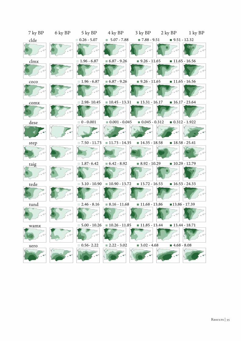
Results |
7 ky BP 6 ky BP 5 ky BP 4 ky BP
clde
clmx
coco
comx
0.26 - 5.07 7.88 - 9.51 9.51 - 12.32
1.96 - 6.87 6.87 - 9.26 9.26 - 11.65 11.65 - 16.56
1.96 - 6.87 6.87 - 9.26 9.26 - 11.65 11.65 - 16.56
2.98- 10.45 10.45 - 13.31 13.31 - 16.17 16.17 - 23.64
3 ky BP 2 ky BP 1 ky BP
dese 0 - 0.001 0.001 - 0.045 0.045 - 0.312 0.312 - 1.922
step 7.50 - 11.73 11.73 - 14.35 14.35 - 18.58 18.58 - 25.41
taig 1.87- 6.42 6.42 - 8.92 8.92 - 10.29 10.29 - 12.79
tede 3.10 - 10.90 10.90 - 13.72 13.72 - 16.53 16.53 - 24.33
tund 2.46 - 8.16 8.16 - 11.68 11.68 - 13.86 13.86 - 17.39
wamx 5.00 - 10.26 10.26 - 11.85 11.85 - 13.44 13.44 - 18.71
xero 0.56- 2.22 2.22 - 3.02 3.02 - 4.68 4.68 - 8.08
5.07 - 7.88
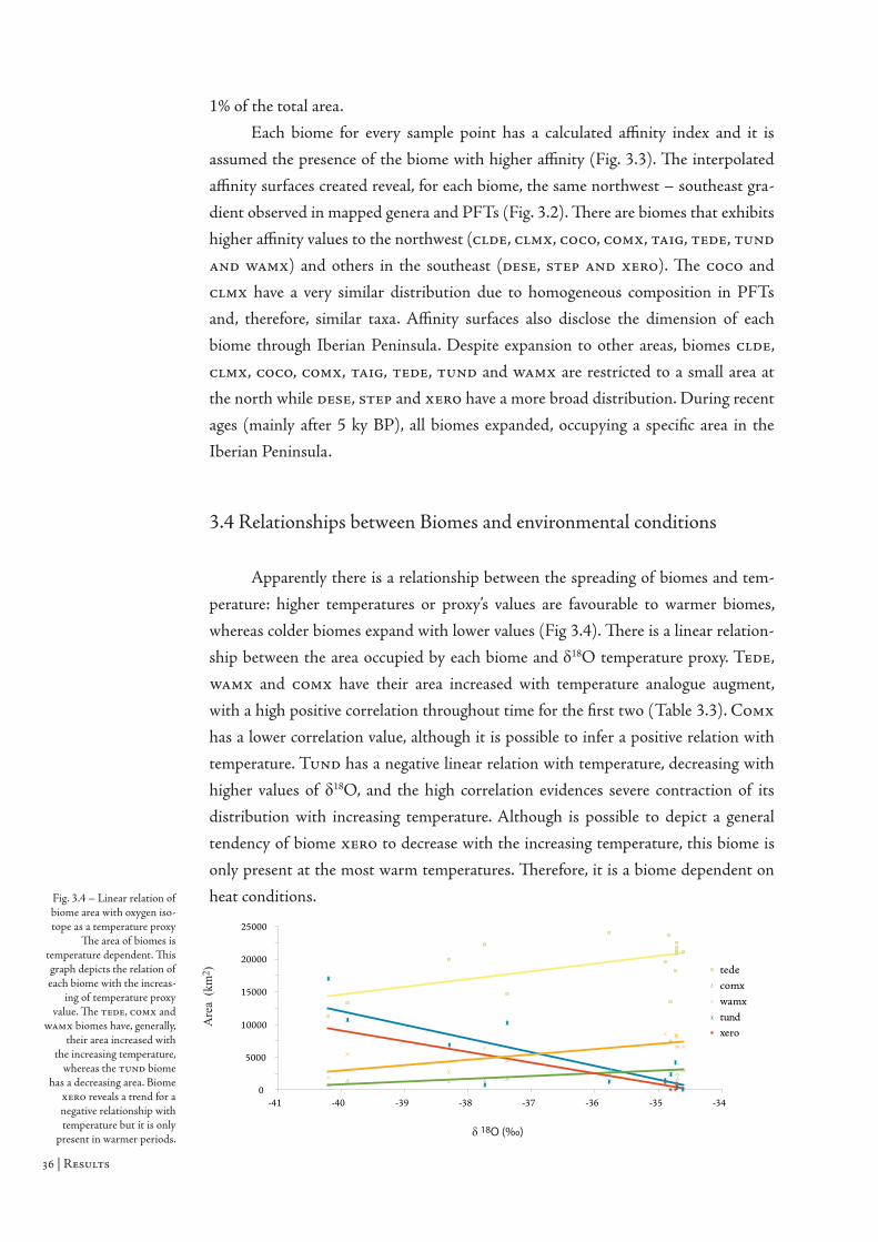
| Results
Apparently there is a relationship between the spreading of biomes and tem-
perature: higher temperatures or proxy’s values are favourable to warmer biomes,
whereas colder biomes expand with lower values (Fig 3.4). Th ere is a linear relation-
ship between the area occupied by each biome and δ18O temperature proxy. Tede,
wamx and comx have their area increased with temperature analogue augment,
with a high positive correlation throughout time for the fi rst two (Table 3.3). Comx
has a lower correlation value, although it is possible to infer a positive relation with
temperature. Tund has a negative linear relation with temperature, decreasing with
higher values of δ18O, and the high correlation evidences severe contraction of its
distribution with increasing temperature. Although is possible to depict a general
tendency of biome xero to decrease with the increasing temperature, this biome is
only present at the most warm temperatures. Th erefore, it is a biome dependent on
heat conditions.
0
5000
10000
15000
20000
25000
-41 -40 -39 -38 -37 -36 -35 -34
tede
comx
wamx
tund
xero
δ 18O (‰)
Are
a (k
m2 )
Fig. 3.4 – Linear relation of biome area with oxygen iso-tope as a temperature proxy
Th e area of biomes is temperature dependent. Th is graph depicts the relation of each biome with the increas-
ing of temperature proxy value. Th e tede, comx and
wamx biomes have, generally, their area increased with
the increasing temperature, whereas the tund biome
has a decreasing area. Biome xero reveals a trend for a negative relationship with temperature but it is only
present in warmer periods.
3.4 Relationships between Biomes and environmental conditions
1% of the total area.
Each biome for every sample point has a calculated affi nity index and it is
assumed the presence of the biome with higher affi nity (Fig. 3.3). Th e interpolated
affi nity surfaces created reveal, for each biome, the same northwest – southeast gra-
dient observed in mapped genera and PFTs (Fig. 3.2). Th ere are biomes that exhibits
higher affi nity values to the northwest (clde, clmx, coco, comx, taig, tede, tund
and wamx) and others in the southeast (dese, step and xero). Th e coco and
clmx have a very similar distribution due to homogeneous composition in PFTs
and, therefore, similar taxa. Affi nity surfaces also disclose the dimension of each
biome through Iberian Peninsula. Despite expansion to other areas, biomes clde,
clmx, coco, comx, taig, tede, tund and wamx are restricted to a small area at
the north while dese, step and xero have a more broad distribution. During recent
ages (mainly after 5 ky BP), all biomes expanded, occupying a specifi c area in the
Iberian Peninsula.

Results |
3.5 Distribution of persistence areas of plant genera
Th e core presence of each genus occurred in distinct locations of the Iberian
Peninsula and the Balearic Islands (Fig. 3.5). Nevertheless, there is a broad pattern
that clusters genus Alnus, Betula, Castanea and evergreen Quercus in the north-
eastern portion of Iberia, while Olea, Pistacia and deciduous Quercus cores dwell in
the south-eastern area. Genus Fagus had the most diff erent location, in the northeast
of Iberian, near the Pyrenees Mountains. In the core of the genus Olea has a noticea-
ble presence in the eastern and southern Iberia, although its presence extends
between those areas. In the Balearic Islands is noticeable the presence of one core of
Olea and, at a lesser extent, Pistacia and deciduous Quercus.
Fig. 3.5 – Stable core areas of each mapped genus.Th e pollen percentage maps of each age were combined together through their aver-age values for each genus. Th e resulting map indicates the constant presence locations of genera from 15 to 1 ky BP. (continues on the next page)

| Results
Fig. 3.5 – Stable core areas of each mapped genus.
continued.

Results |
DiscussionDeglaciation was not a monotonic event (Alley & Clark 1999, Folland et al. 2001).
Th erefore, the shiftable patterns throughout time of vegetation distribution in the
Iberian Peninsula were expected and confi rmed with the present work. In the
Balearic Islands, the distribution of vegetation and range shifts follow the same pat-
terns as south-eastern Iberia. Th ese shifting patterns of vegetation persistence and
migrations during the late-Quaternary exposed in this study are coherent with other
world and European scale reconstructions (Prentice et al. 1996, Elenga et al. 2000),
climate change (Grootes et al. 1997, Heiri 2003), predictions of vegetation presence
(Garzón et al. 2007), historical facts (Conedera at al. 2004) and molecular phyloge-
nies (Belaj et al. 2007, Besnard et al. 2002, 2007, Dumolin-Lapègue et al. 1997,
Fineschi et al. 2000, King & Ferris 1998, Kropf et al. 2006, Lumaret et al. 2004,
Magri et al. 2006, Maliouchenko et al. 2007, Olalde et al. 2002, Palme et al. 2003,
Petit et al. 2002, 2005, Taberlet et al. 1998).
During the late-Quaternary in the Iberian Peninsula, Steppe was a dominant
biome, as previously reported to Mediterranean areas with a probable savannah type
structure like those that can be found nowadays in arid areas of Spain (Elenga et al.
2000). Th is dominance is due to presence of high number of families with low pollen
percentages. As Prentice (1996, 1998) asserted, the square-root included in equation
used to calculate biome affi nity maximize the detection of low abundance taxa.
Th erefore, a high value of affi nity to Steppe was expected, as minor indicator taxa is
valuable to the biomization method. Th is comprises families as Chenopodiacea,
Poaceae and genus like Artemisia that have a high number of species and a widely
distribution in sample points, thus, despite the low pollen percentage values, a high
affi nity is achieved as a consequence of the assignment of numerous vegetation types
to biome Steppe (Elenga et al. 2000). Furthermore, the affi nity scores originated
from digitized data could be biasing the scores for this biome due to lower resolution
of minor taxa pollen. Raw pollen counts should be used to better assess the affi nity
score.
Th e second best affi nity scores reveal that the temperate deciduous and cool
mixed forests were dominants in Iberian Peninsula since 15 ky BP. Extreme winters

| Results
along with arid summers may have reduced the distribution of Mediterreanean ever-
green trees and shrubs, resulting in Steppe arising at high altitude lakes (Elenga et al.
2000, Prentice et al. 1992). For biome mapping, Steppe was excluded to enhance
perception of evolving biomes distribution and area occupied in each time frame.
Elenga et al. (2000) highlighted the important information provided from these
runner-up biomes for the analysis of vegetation dynamics in Western Europe and
suggested a further division or diff erent classifi cation of treeless biomes.
A modern biome map was adapted from literature due to limitations with the
available number of sites with data for present. Moreover, anthropogenic factors have
a strong eff ect in biomes classifi cation, misleading it. Heatlands in southern Europe
are usually misidentifi ed as Tundra due to presence of Ericales, Poaceae and
Cyperacea pollen, which are indistinguishable at a biome scale (Prentice et al. 1996).
Th e number of available data points is a major constrain in this type of re-
constructions. In the present study, this was counterbalanced by a reasonable geo-
graphic distribution of pollen sites. Th is non uniform distribution left a low sampled
area in southwestern Iberian Peninsula. Th is area comprises the southern plateau
and it is topographically homogenous, thus it is not expected great variation in its
vegetation composition at each age, and the available data should allow good predic-
tions. Areas with more heterogeneous terrains have normally a good composition of
sampled points. Th us, small variations due to the presence of more possible natural
barriers to climate and dispersion should be predicted. Another constrain of this
strategy to reconstruct past environments is the non-stability of available points
throughout time. Some data have a higher temporal resolution and extended the
provided information throughout almost all timescale, while others represent just a
small portion. Th ese latter data were used to balance missing data in some locations
and at some ages, otherwise it was used to increase the resolution of the analysis.
Th erefore, it was chosen for analysis a timescale between 1 and 15 ky BP derived
from the limitation of available points, while taking into account their geographic
distribution.
Th e data used to yield distribution maps, the fossil pollen record, has some in-
herent diffi cult issues to deal, such as the unknown relationships between pollen
data and the density of mother plants (Odgaard 1999). Th erefore it is an extremely
complex task to extract densities from pollen records. Nevertheless, fl uctuations in
the amount of pollen found in sampled locations for the same taxa are indicative of
higher or lower presence throughout time. Furthermore, fi nding pollen of one taxon
or assemblage is an incontestable evidence of its presence at some age. Th e rapid
change of tree presence and migrations is perceived within the thousand year interval
as response to climate. Th ose changes were not constant at spatial and temporal di-
mensions (Clark 1998). Using the available paleovegetation data it is possible to vali-
date of the information internally due to the spatial autocorrelation of biological data

Discussion |
throughout time: geographic closer points at certain age have similar pollen compo-
sition. Th is is refl ected in the consistent patterns of paleopollen distribution. Despite
all pollen associated issues, such as accurate calibration and suffi cient density of sites,
this is a valuable source of information for past vegetation composition and histori-
cal factors (Petit et al. 2004).
Ecological information is lost in the transformation of pollen data to biome
maps (Williams et al. 2004) but this method presents several advantages that are
useful to compare between diff erent zones of the world, timescales and methods.
Th e synthetic information provided enlightened areas of congruent climatic and veg-
etation features. Also they not necessarily rely on large data sets of data to yield
results (Prentice et al. 1996, Prentice et al. 1998), like is often the case of paleovege-
tation reconstruction. Th e intermediate stage between the assignments of taxa to
biomes is the classifi cation in PFTs. Th is classifi cation is sensible to changes in vege-
tation and biodiversity as consequence of environmental shifts at diff erent scales
(Rusch et al. 2003) and, taken together, the classifi ed taxa represent a very character-
istic climate range.
4.1 Correlations with climate data
Th e late-Quaternary, as already seen, was a period of intense climatic oscillations,
ranging from the LGM to modern temperatures, with abrupt changes and fl uctua-
tions. Th e analysis of the relationship between temperature abnormalities and the
occupied areas by each biome reveals the major events of the Holocene (Fig. 3.2 and
3.3). Th ese events had an extreme importance in the evolving patterns of vegetation
distribution, producing expansion and retraction phases and the consequent sudden
emergence and extinction of biomes. Imprints of climate shifts are evident and as-
sessable through the distribution maps.
Oldest dryas and Bölling-Alleröd – From LGM to the fi rst warming phase
Th e peak of last glacial maximum was at ~18 ky BP in the Pleistocene, and
the transition to full-interglacial period begun since then to 10 ky BP, which is
known as the Bölling-Alleröd warm period (Folland et al. 2001, Roberts 1998). Th e
contraction of tundra distribution was noticeable during this warming period along
with an expansion of temperate forests (Fig. 3.2). Th e cold mixed forests remained
in the north, with slight shifts in their distributions, mainly with eastern orientated
movement. Th e area occupied by warm mixed forest decreased towards southeast,
being occupied by the temperate forest. During this period, the biome steppe mi-
grated to the southwest (for individual biome surfaces, see Fig. 3.3), indicating a con-

| Discussion
traction of treeless biomes. Plant associations point towards a migration of warmer
assemblages from eastern to southern Iberian Peninsula and a fast reduction of tree-
less PFTs (Fig. 3.2). Th e PFT bs has the most obvious shift: at the maximum age
studied, it had its presence confi ned to northern Iberian Peninsula and at 13 ky BP
expanded throughout almost all peninsula. Th is warming phase was also character-
ized by movements of individual genera (Fig. 3.1). Genus as Betula and Castanea ex-
panded their distribution in the Iberian Peninsula, the latter with a pattern similar
to those achieved with predictive modelling with climatic data for the last glacial
maximum (Garzón et al. 2007). It was not possible to model Fagus at this period due
to limitation of evidences from pollen. Huntley (1989) suggested a restricted distri-
bution of beech during the Holocene, possible in refugia in the Balkanic and the
Italic Peninsulas, expanding and reaching Iberia in recent times (~4 ky BP).
Although it was not possible to achieve a distribution of deciduous Quercus species
at latter times, its expansion is perceptible at 13 ky BP, occupying most of the western
belt of Iberia. Th e comparison of pollen percentages between diff erent genus is
almost impossible due to diff erent pollen production (Odgaard 1999). However, it is
possible to conclude, based on the time-series analysis of the same genus, that ever-
green Quercus had a weak appearance in this period and a slight retraction at 14 ky
BP.
Th e end of Pleistocene marks the beginning of a warmer, although unstable
climate. During the LGM, species found their refugia mainly in the north and south
of the Iberian Peninsula and the warming gave birth to a continuous shift of occu-
pancy by each genus, assemblages and biomes. Th is conspicuous relation of patterns
of migration and climate is assessed through the distribution maps and correlations
between areas and temperature proxies.
Younger Dryas – Return to cold
Th e following event is characterized by a reversal in temperature trend, drop-
ping to very low values and originating cold, dry and windy conditions when com-
pared to the present (Alley & Clark 1999). Th is period known as Younger Dryas ex-
tended from ~12 to 11.5 ky BP (Folland et al. 2001, Isarin 1997), and the main
evidence in fossil pollen is the restoration of Tundra predominance in Iberian
Peninsula while this event occurred (Fig. 3.2). Th e temperate forest was pushed to
northern Iberia and there was a small southern refuge for the warm mixed forest.
Betula species had a minor increase of their distribution area during this period,
being the only genus to expand southwards (Fig. 3.1). Pistacia had a longitudinal
shift, with increased presence of pollen in the south, in the same area of warm mixed
forest. Both evergreen and decidous Quercus have their area decreased to a minimum

Discussion |
expression of pollen, the former in the south and the latter in the northwest. Th ere is
no great impact on bs PFT suggesting a good response to colder climates, as oppo-
site to ts and wte PFT that have a reduction of their areas with a similar pattern
of deciduous and evergreen Quercus, respectively. Th e Castanea species had a large
reduction, occupying during this period a small refugee in northern Iberia.
Th e Younger Dryas is a paradigm of late-Quaternary trend reversal with
abrupt transitions. As seen in the mapped distributions here, it has a major impact
on plant dispersal despite their ephemeral nature when compared to most persistent
climatic trends.
Holocene - Warmer beginning
A warmer period followed the Younger Dryas, characterized by an excep-
tional retraction of Tundra and expansion of warmer biomes (Fig. 3.2). During this
period occurred the fi rst appearance of the hottest biome, Xerophyte, in the south of
Peninsula. It ranged in areas previously occupied by Warm mixed forests and it was
surrounded by this biome. Th e persistence of both these biomes is a clear sign of a
permanently warm region. Th e Cool mixed forest and its co-dominance with
Temperate deciduous forests have the most mutable distribution during this event:
it shifted from a northwestern distribution to a north and eastern cores at 10 ky BP
and with posterior dominance in the east. Between 10.7 and 10.5 ky BP occurred a
fast cooling event, detected in the Swiss alps in inferred July air temperatures (Heiri
et al. 2003), with a perceived eff ect in Iberian Peninsula due to expansion of Tundra
near Serra da Estrela (Portugal) and Valencia (Spain) and decreased area of Warm
mixed forests.
At 9 ky BP there was a evolution of Xerophytic and Tundra biomes with an
improbable proximity. Th is could be due to the nature of interpolations and pollen
analysis: the collection sites are often lakes or peat bogs that collect pollen from a
wide area and may confound regional an local eff ects (Williams et al. 1998).
Th erefore, Tundra composition is possible restricted to high altitude lakes at colder
time and its presence could be extended to other areas by pollen dispersion and in-
terpolations results. Nevertheless, it was notorious the dominance of treeless biomes
in the southeastern area of Iberia. Th e PFT wte is very sensible to temperature
changes: during this cold event it is noticeable a narrowing of its distribution to the
warmer areas of southern Iberia, while during warmer periods it extends throughout
all Iberia. Th e PFTs bs and ts have a distribution pattern similar to the temperate
bioclimatic zone, and the warmer sf and wte PFTs are similar to Mediterranean
bioclimatic zone (Fig. 2.2). Th e main warmer trend of this period caused a retaction
of Betula species from the southeast and an abrupt change in Olea species distribu-
tion during the small cold event, when it spreaded along a narrow area in the

| Discussion
Mediterranean coast (Fig. 3.1). Th e deciduous Quercus species had a noticeable pres-
ence in the northwest, with high percentage of pollen when compared to the
maximum achieved throughout the studied timescale and spreaded southwards
during this period. Evergreen Quercus persisted in the south with low values and
even with undetectable cores during the cold event but has an expansion to almost
all Iberia area at 9 ky BP. With a similar pattern, Castanea had a strong retraction
that resulted in undetectable cores at 10 ky BP. Th e fi rst evidence of genus Fagus suggests a core in the north and further expansion, always with low levels of pollen
percentage. Th e warmer climate of the Holocene should have boosted the dispersion
of these warmer species.
Cold event at 8.2 ky BP - Sudden reversal
As already seen, even fast climatic reversals may have a strong impact in vege-
tation dispersal. At ~8 ky BP a shift in temperature was triggered, producing a
cooling event even faster than the Younger Dryas (Baldini et al. 2002, Rohling &
Palike 2005). Th is event aff ected the distribution of biomes, and Tundra expanded
again along with Cool mixed forests (Fig. 3.2). Warm mixed forest remained with
unnoticeable changes, probably due to the brisk appearance of this event. Th e cooling
climate had a strong infl uence in the treeless biomes as seen in the expansion of
Tundra and in Steppe which has discontinued its reduction drift during this event.
As in previous cooler climates, the wte presence was reduced to the southern
Iberia, while other PFTs did not had considerable shifts in their distribution (Fig.
3.2). Th erefore, the impact of cooler climates shifts, especially in warmer trend ages,
is stronger in the mostly thermophilic species. Th is seems to be the case of Olea,
since it proved to be very sensible to climatic fl uctuations (Fig 3.1). For instance, in
the presence of fast cooling events, its distribution was systematically reduced to
small areas in the Mediterranean coast. Both mapped Quercus were more resilient to
this sudden reversal in climate, maintaining their distribution with slight changes.
Holocene Maximum Warming - Th e current warming phase
Th e Holocene maximum warming phase in Europe extended from 6 to 4.5
ky BP and Temperate deciduous and Warm mixed forests have prevailed during this
time (Fig. 3.2). From 4 ky BP until now, there were temperature shifts that caused
the emergence of cold and arid biomes. At 6 ky BP there was a subtle decrease in
temperature which left imprints in the most sensible distributions: the PFT wte
and the genus Olea distributions had a sudden decrease as already seen in other
cooling events (Fig. 3.1).
Genus Castanea had a drastic decrease from its constant presence in the north-

Discussion |
west to a subtle core. Due to extreme low values of pollen percentage and narrow
presence, the uncertainty in the presence of this core does not diff er from the pres-
ence of the genus during this millennium. Although, it reappears at 5 ky BP in the
same location with high values, suggesting a remaining founder core. Th e strong
presence in the northwest contrast with the broad distribution of Castanea at 2 ky
BP. Th is age marks a new period in the history of Iberian Peninsula: the arrival of
Romans in the southeast coast at 220 BC and successful journey during the second
Punic Wars which led to the control of all Iberia even before 200 BC. Th e spread of
Roman civilization throughout Iberia consequently implied the spread of their agri-
cultural habits as the cultivation of Castanea sativa for medicine, wood and food
(Conedera et al. 2004). Th e knowledge about Castanea sativa fruit eff ects have been
described in the ancient Greek. Athenaeus (translated by Yonge, 1854), citing previ-
ous authors addresses the subject in a humoristic way: “...Mnesitheus the Athenian, in his book on Comestibles, says, ‘ Th e digestion of Eubuean nuts or chestnuts (for they are called by both names) is very diffi cult for the stomach, and is attended with a great deal of fl atulence, and they are apt to thicken the juice, and to make people fat, unless their consti-tution is strong enough to neutralise them’”.Th e long history of human induced distri-
bution of Castanea sativa was confi rmed by historical and genetic analysis (Fineschi
et al. 2000). Th erefore, the vast dispersal of this genus was mostly due to human
factors. Furthermore, the same impact could be expected in other species; for in-
stance, the more subtle changes in species Olea during 1 ky BP.
Th e emergence of Tundra biome at 1 ky BP has a dual interpretation: lower
temperatures and/or anthropogenic factors. Temperature alone does not completely
justify the presence of Tundra in a great area since there was a weak lower tempera-
ture anomaly in a more general warm tendency and Tundra did not aroused as
widely as in other colder periods. Prentice (1996) advanced a possible human factor
in the emergence of biome Tundra during modern times: the presence of Ericales,
Poaceae and Cyperacea pollen is characteristic of anthropogenic heatlands and, al-
though with diff erent compositions, heatlands produce indistinguishable pollen from
Tundra. Heatlands may thus counfound pollen counts and be responsible for an ar-
tifi cial increase of Tundra.
Th e presence of Xerophytic biome at 1 ky BP is indicative of a warmer climate
in the Mediterranean area of the Iberian Peninsula, with the nowadays characteristic
arid zones.
4.2 Comparing independent past landscape reconstructions
One of the main advantages of mapping biomes is the possibility to compare between
several other worldwide or regional biomes from diff erent sources. Th e mapped dis-

| Discussion
tribution of pollen percentage is also an excellent tool to compare with other proba-
ble distributions of species for the late-Quaternary. Th is advantage steams from pat-
terns of biomes, plant associations and individual genus being perceived in the time
series of mapped distributions. A similar outcome was found in North America by
Williams (2004) during a similar time span analysis with emergence and disappear-
ance of biomes. Plant associations and individual genus also responded to climatic
shifts with a constant variation of distribution in North America during late
Quaternary oscillations. Th e vegetation patterns have a dynamic equilibrium with
climate, which is an assumption for modelling pollen distribution. With the fi ner
scales normally used in plant ecology it is diffi cult to assume this equilibrium due to
non equilibrium processes as succession in plants. However, with larger spatial and
temporal scales the main patterns of distribution refl ect the climate driven shifts
(Prentice et al. 1991).
In a biome reconstruction for 6 ky BP in Europe (Prentice et al. 1996) it was
suggested colder winters then present together with wetter conditions at growing
season, accompanied by the replacement of today’s Xerophytic vegetation by temper-
ate forests in the Mediterranean region. Th ese past conditions are supported by the
present study in the Iberian Peninsula. At 6 ky BP, Iberia was characterized by the
dominance of Temperate forests along with Warm mixed forests at a lesser extent,
and with a small appearance of cool forests in the north. Th is combination of biomes
was stable for this warming phase.
At the LGM, it was predicted a dominance of Steppe in Mediterranean region,
including Iberia in a pollen analysis of past biomes for Europe and North Africa
(Elenga et al. 2000). Th is is also supported in this study. As discussed before, the
dominance of Steppe is ambiguous and the biomes with the second highest affi nity
Fig. 4.1 – Geographic per-sistence of taxa
Th e reconstruction of taxa distributions allowed the il-
lustration of areas where they have always occurred. Th ose
areas of persistence, shown in the map with diff erent
colours and line styles, are divided into two main areas: one at the Temperate region and other at the Mediterra-
nean region.
Fagus
AlnusBetulaCastanea
PistaceaQuercus (deciduous)
Quercus (evergreen)
±0 100 200 400
Km
Olea

Discussion |
scores usually provide better information about vegetation changes in Iberia. Tundra
and cool biomes were widespread in central Europe. Nevertheless, in lower latitudes,
there was an increasing supremacy of Temperate forests. Furthermore, in Turkey, at
the same latitude of southern Iberia, there was a clear preponderance of this type of
forests during the LGM at 18 ky BP. Th erefore, at 15 ky BP it were expected in the
Iberian Peninsula the presence of Tundra as in central Europe, Italy and the
Temperate forests of European lower latitudes.
Th e comparison of diff erent data sources is worthy to detect fl aws in past re-
constructions. Th e paleopalynology data is a good benchmark to evaluate simula-
tions (Huntley 2001). Th e relationship between past biomes and vegetation mapping
with independent data of temperature proxies is compared along the present study
with success. Th is comparison allowed the detection of the main patterns of climate
shifts in plant migrations. Th e next step is to compare the present reconstruction
with others built with diff erent climatic modelling approaches. Jost (2005) found
some discrepancies for Western Europe between climate simulations and tempera-
tures obtained by pollen models. Th ose diff erences, although reduced, were found
even with higher resolution simulations. Some reconstructions of past landscapes
use climate simulations to predict distribution of species in the past (Williams et al.
1998). Although the pollen distribution assumes a constant equilibrium with
climate, despite other small scale processes, the predictive approach uses present dis-
tribution to simulate past ranges. Th is implies that the actual spread of species are
human independent. However, some economic valuable species have distributions
extended to their physiologic limits while others have shrunken their potential dis-
tribution. Th e Castanea sativa have an unambiguous human infl uence in its distribu-
tion since 2 ky BP. Th is factor imposes a great eff ort to model correctly the past dis-
tribution. In a predictive modelling approach to the past landscape in Iberian
Peninsula this problem was partially avoided by correlating with the current Iberian
natural forests (Garzón et al. 2007). Th e results found are compatible with the
current work at near the LGM and mid-Holocene.
Garzón et al. (2007) found possible refugia in the northwest and the foothills
of the Pyrenees for trees species. Th ese locations were, in the present study, inditifi ed
also as areas of constant presence throughout time for several tree species (Fig. 4.1),
where the mountain topography is most likely to create a favourable environmental
situation for the maintenance and diff erentiation of genetic structure (Magri et al.
2006). But the present study identifi ed also persistence areas in southern Iberia for
Mediterranean species (Olea and Pistacia) not predicted by Garzón et al. (2007). Th e
higher accuracy of the present study is probable a consequence of the analysis not
being limited to the spatial and temporal resolution of climate simulations.
Biomization procedure and interpolated pollen percentages surfaces have a temporal
sequence that allows discerning migrations.
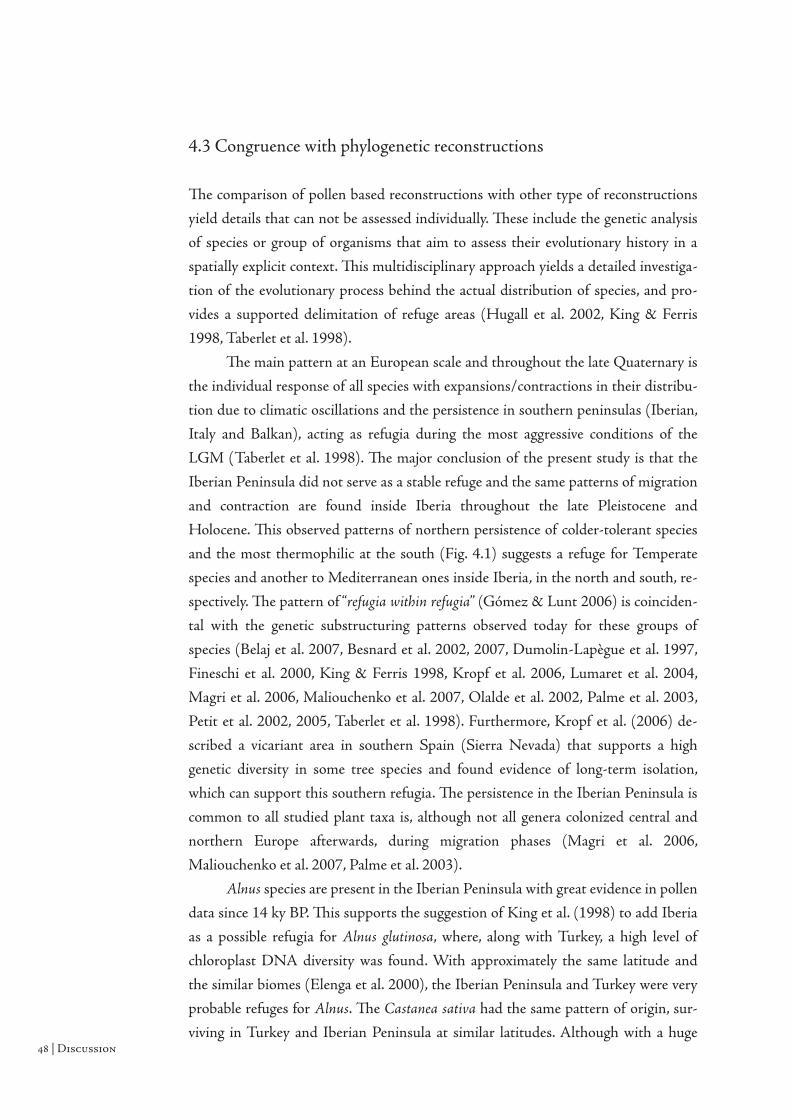
| Discussion
Th e comparison of pollen based reconstructions with other type of reconstructions
yield details that can not be assessed individually. Th ese include the genetic analysis
of species or group of organisms that aim to assess their evolutionary history in a
spatially explicit context. Th is multidisciplinary approach yields a detailed investiga-
tion of the evolutionary process behind the actual distribution of species, and pro-
vides a supported delimitation of refuge areas (Hugall et al. 2002, King & Ferris
1998, Taberlet et al. 1998).
Th e main pattern at an European scale and throughout the late Quaternary is
the individual response of all species with expansions/contractions in their distribu-
tion due to climatic oscillations and the persistence in southern peninsulas (Iberian,
Italy and Balkan), acting as refugia during the most aggressive conditions of the
LGM (Taberlet et al. 1998). Th e major conclusion of the present study is that the
Iberian Peninsula did not serve as a stable refuge and the same patterns of migration
and contraction are found inside Iberia throughout the late Pleistocene and
Holocene. Th is observed patterns of northern persistence of colder-tolerant species
and the most thermophilic at the south (Fig. 4.1) suggests a refuge for Temperate
species and another to Mediterranean ones inside Iberia, in the north and south, re-
spectively. Th e pattern of “refugia within refugia” (Gómez & Lunt 2006) is coinciden-
tal with the genetic substructuring patterns observed today for these groups of
species (Belaj et al. 2007, Besnard et al. 2002, 2007, Dumolin-Lapègue et al. 1997,
Fineschi et al. 2000, King & Ferris 1998, Kropf et al. 2006, Lumaret et al. 2004,
Magri et al. 2006, Maliouchenko et al. 2007, Olalde et al. 2002, Palme et al. 2003,
Petit et al. 2002, 2005, Taberlet et al. 1998). Furthermore, Kropf et al. (2006) de-
scribed a vicariant area in southern Spain (Sierra Nevada) that supports a high
genetic diversity in some tree species and found evidence of long-term isolation,
which can support this southern refugia. Th e persistence in the Iberian Peninsula is
common to all studied plant taxa is, although not all genera colonized central and
northern Europe afterwards, during migration phases (Magri et al. 2006,
Maliouchenko et al. 2007, Palme et al. 2003).
Alnus species are present in the Iberian Peninsula with great evidence in pollen
data since 14 ky BP. Th is supports the suggestion of King et al. (1998) to add Iberia
as a possible refugia for Alnus glutinosa, where, along with Turkey, a high level of
chloroplast DNA diversity was found. With approximately the same latitude and
the similar biomes (Elenga et al. 2000), the Iberian Peninsula and Turkey were very
probable refuges for Alnus. Th e Castanea sativa had the same pattern of origin, sur-
viving in Turkey and Iberian Peninsula at similar latitudes. Although with a huge
4.3 Congruence with phylogenetic reconstructions

Discussion |
human infl uence on its distribution, the historical origin of Castanea sativa is attrib-
uted to Turkey along with other possible refugia in northwestern Iberia, as suggested
by phylogenetic analysis (Fineschi et al. 2000). Th is study provides additional sup-
porting evidence of this northwestern Iberian refuge, very sensible to climate
oscillations.
Th e genus Betula is clearly a case of a cold-tolerant species surviving at lower
latitudes during the LGM, although its main refugia core were at higher latitudes
(Maliouchenko et al. 2007, Palme et al. 2003). Th e proposed refugia for those species
are northern Alps, southern Sweden and areas close to the Ural Mountains (Palme
et al. 2003). Th ere is a strong pollen evidence for a northwestern Iberia persistence
of this genus with posterior expansion during the late Quaternary, even though they
are unlikely to be the source for colonization of central and northern Europe after
the LGM (Maliouchenko et al.).
Molecular studies of Olea species point to a dual origin in the west and east of
the Mediterranean Basin with some degree of separation in the western populations
(Besnard et al. 2002, 2007). Th e complex biogeography history of olive populations
in the Mediterranean, due to environmental factors and human dispersion, contrib-
uted to populations diff erentiation (Besnard et al. 2002). In the present work, it is
possible to notice the constant presence of Olea species in southern Iberia and its
thermophilic characteristic with extensive responses to climate change: expansion
during warmer phases and contraction in colder periods. Besnars et al. (2007) sug-
gested that during the LGM, which was a favourable period for olive in North Africa,
there may have been gene fl ow between these populations and the ones from the
Mediterranean basin.
In an extensive study of Fagus distribution in North America and Europe,
Huntley et al. (1989) suggested a restricted distribution to Italy and Balkans at the
LGM. Th e following expansion from those refuge areas reached Iberian Peninsula
through the Pyrenees Mountains at 4 ky BP. At this age there is an obvious increase
in pollen percentage of Fagus genus near the Pyrenees, indicating a more stable pres-
ence in that area, probably due to expansion from described refuge. Nevertheless,
this genus is constantly present in North Iberia throughout the time span of the
present study. A haplotype found in Cantrabrean Mountains support the evidence
of persistence of Fagus, and there is isozyme evidence of three populations in this
area during the Holocene, although they did not contribute for the colonizing of the
rest of Europe (Magri et al. 2006).
Th e fossil pollen analysis does not often reach higher taxonomic levels for
Quercus than the classifi cation in deciduous or evergreen. As seen, these diff erent as-
semblages have diff erent persistence in Iberian Peninsula since the LGM: the ever-
green residing at the south, whereas the deciduous dwell at the northwest. Th e
Iberian refugia is obvious in molecular analysis of white oaks in Europe, due to the

| Discussion
presence of high chloroplast DNA diversity (Dumolin-Lapègue et al. 1997, Olalde
et al. 2002, Petit et al. 2002). Inside the Îberian Peninsula, however, molecular data
reveals a complex pattern of migrations during the Holocene with diff erent smaller
refugia (Olalde et al. 2002, Petit et al. 2002). Th is is compatible with the present
results, where migrations inside the peninsula have visible patterns in the fossil
pollen presence. Moreover, the suggested routes for lineages migration inside the pe-
ninsula and the migration inwards (Olalde et al. 2002, Petit et al. 2002) are congru-
ent with the pollen evidence: 1) deciduous Quercus have fi rst appearance in central/
south Portugal at 13 ky BP, followed by a migration to north, prevailing in the north-
west with an extension towards the Pyrenees; 2) the evergreen Quercus have a south-
ern dominance, expanding to central Iberia and a slight change of their main core
eastwards, along the Mediterranean coast.
Olalde (2002) suggested that the latitudinal eff ect in the Iberian Peninsula is
overridden by its topography, creating possible refugia both in northern and south-
ern areas.
4.4 Parallelism between fauna and fl ora refugia
Th e glacial refugia areas for fauna and fl ora are obviously related due to a common
vicariant history (Gómez & Lunt 2006). Although there is a lack of geographic reso-
lution when defi ning refugia areas in most studies (Gómez & Lunt 2006), the
Mediterreanean and Temperate refuge described in this study exhibit a parallelism
with the fauna refuge described by several genetic studies (Fig. 4.2). In Northern
Iberia there is evidence for several refugia for fauna species along with the Alnus, Betula, Castanea, Fagus and deciduous Quercus refugia proposed in this study. In
Picos de Europa Mountains there is some genetic evidence for herpetofauna refugia,
including Zootoca vivipara (Guillaume et al. 2000, Surget-Groba et al. 2001) and
Salamandra salamandra (Garcia-Paris et al. 2003, Steinfartz et al. 2000); and
mammals, Lepus castroviejoi (Pérez-Suárez et al. 1994).
Th e Central Mountain System is proposed as a refugia for Lacerta schreiberi (Paulo et al. 2001, 2002), Chioglossa lusitanica (Alexandrino et al. 2000, 2002), Alytes obstetricans boscai (Arntzen & Garcia-Paris 1995, Fonseca et al. 2003) and Microtus agrestis ( Jaarola & Searle 2002). In the present study, this area does not have a con-
tinuous strong presence of pollen data when confronted to both persistence cores in
the north and south (Fig. 4.1). Nevertheless, Betula and Alnus at a lesser extent, are
present it the Central System throughout the late-Quaternary, indicating a possible
continuous presence there. Although their persistence areas have an evident core in
the northern Iberian Peninsula, those are the genus with persistence areas extending
further south, reaching the Central System (Fig. 3.5).

Discussion |
In southern Iberian Peninsula putative refugia for Mediterranean vegetation
was demonstrated in the present work by the continuous presence of evergreen
Quercus, Pistacia and Olea taxa. Th e Baetic Mountains constitute also putative
refugia for several fauna species: Alytes dickilleni (Arntzen & Garcia-Paris 1995),
Discoglossus jeanneae (Garcia-Paris & Jockusch 1999), Salamandra salamandra
(Garcia-Paris et al. 2003, Steinfartz et al. 2000) and Oryctolagus cuniculus (Branco et al. 2000, 2002). Th e latter mammal species has also a possible glacial refugia in the
Ebro basin (Branco et al. 2000, 2002) along with Brachionus plicatilis (Gómez et al. 2000), which is an area with strong presence of Olea species during the
late-Quaternary.
In the Pyreenes, the occurrence of some tree species, as suggested by the dis-
tribution of Olea and Fagus since the LGM, is congruent to other recognized refugia
as indicated for Zootoca vivipara (Guillaume et al. 2000, Surget-Groba et al. 2001).
Th ere is a strong correlation of glacial refugia for fauna described by several
molecular studies and the mapped distribution of vegetation and persistence areas
described in the present study. As Goméz & Lunt (2006) pointed, further studies
are important to delimit and increase the possible refugia areas. Th ese studies may
opt for a molecular approach of several key species in the Iberian Peninsula, or may
be reconstructions based in other evidence as this study demonstrated.
Fig. 3.2 – Glacial refugia for fauna and fl ora in the Iberian PeninsulaTh e climate oscillations force species migrations inside the Iberian Peninsula. Th e arrows indicate possible patterns of migrations for the vegetation, accordingly to pollen data presented in this study. Th e inset boxes indi-cate the putative refugia for several faunal species based on Goméz & Lunt (2006).
Alnus / BetulaAlnus / Castanea / Quercus (dec)
Alnus
Fagus
Olea / Pistacia / Quercus (evr)
Olea
Ole
a
Salamandra salamandraLepus castroviejoiZootoca vivipara
Lacerta schreiberiChioglossa lusitanica
Alytes obstetricans boscaiMicrotus agrestis
Alytes dickilleniDiscoglossus jeanneaeOryctolagus cuniculus
Salamandra salamandra
Brachionus plicatilisOryctolagus cuniculus
Zootoca vivipara
40º
45º
-10º -05º 00º
-05º 00º 05º
40º
35º
Picos de Europa
Central System
Baetic System
Ebro basin
Pyrenees

| Discussion

Conclusions |
ConclusionsIberian Peninsula is usually assumed as one of the southern refugia in Europe for
the adverse conditions of the last glacial epoch. Its low latitude location, when com-
pared to remaining Europe, allowed a more tolerant climate although was aff ected by
the same instability processes, resulting in a dynamic environment throughout the
late Quaternary. Th is makes the Iberian Peninsula a privileged area for analysing the
oscilation processes during the warming since LGM and their infl uences in organ-
isms. As Huntley (2001) suggested, the targets of these analyses should be regions
and times where there is supposed to exist sensible responses to climate shifts. Th e
biomization is a robust method to envisage past vegetation processes through the
fossil pollen data due to high correlation to climate. Moreover, biomization allows
the mapping of distributions of typical taxa and plant assemblages. It was also
stressed the ability of this type of reconstruction to serve as benchmarks for other
methods. Pollen reconstructions and biomization were successfully compared to
direct climate reconstructions as well as with molecular studies identifying probable
refugia. Th e combination of these distinct methods provides a solid understanding
of past processes, mainly when the reconstructions provide a time sequence that
allows visualizing the migrations patterns of taxa.
One of the limitations of the present study is the availability of pollen infor-
mation in digital format. Th e EPD provides a vast database for all Europe with raw
pollen counts which are the best data to reconstruct biomes. Nevertheless, there are
numerous local scale studies that present important pollen data. Th e process of digi-
tizing these data from old and newer pollen cores into general purposes databases
should be encouraged as they constitute important resources providing extremely
useful information to several multidisciplinary studies.
Th e present study also consolidates the usefulness of GIS for the reconstruc-
tions of past environments, as they intrinsically have a spatial content and the display
and analysis in a spatially explicit context provides more detailed information. An
advantage of GIS software is the possibility of developing scripts to automate proc-
esses. Th e eff ort of producing a large number of maps for the present work was
reduced by the development of several scripts that automated cyclic tasks and analy-
sis of results.

| Conclusions

References |
ReferencesAlexandrino, J.; J. W. Arntzen & N. Ferrand (2002). Nested clade analysis and
the genetic evidence for population expansion in the phylogeography of the
golden-striped salamander, Chioglossa lusitanica(Amphibia: Urodela). Heredi-ty, 88(1): 66-74
Alexandrino, J.; E. Froufe; J. W. Arntzen & N. Ferrand (2000). Genetic subdivision,
glacial refugia and postglacial recolonization in the golden-striped salamander,
Chioglossa lusitanica (Amphibia: Urodela). Molecular Ecology, 9(6): 771-781
Alfano, M. J.; E. J. Barron; D. Pollard; B. Huntley & J. R. M. Allen (2003). Com-
parison of climate model results with European vegetation and permafrost
during oxygen isotope stage three. Quaternary Research, 59(1): 97-107
Alley, R. B. & P. U. Clark (1999). Th e deglaciation of the northern hemisphere: A
global perspective. Annual Review of Earth and Planetary Sciences, 27: 149-182
Alley, R. B.; P. A. Mayewski; T. Sowers; M. Stuiver; K. C. Taylor & P. U. Clark
(1997). Holocene climatic instability: A prominent, widespread event 8200 yr
ago. Geology, 25(6): 483-486
Anderson, N. J.; M.-J. Gaillard; H. Bugmann & J. A. Dearing (2006). Linking
palaeoenvironmental data and models to understand the past and to predict
the future. Trends in Ecology & Evolution, 21(12): 696-704
Arntzen, J. W. & M. Garcia-Paris (1995). Morphological and allozyme studies of
midwife toads (genus Alytes), including the description of two new taxa from
Spain. Contributions to Zoology, 65: 5-34
Augustin, L.; C. Barbante; P. R. F. Barnes; J. M. Barnola; M. Bigler; E. Castellano;
O. Cattani; J. Chappellaz; D. Dahl-Jensen; B. Delmonte; G. Dreyfus; G.
Durand; S. Falourd; H. Fischer; J. Flückiger; M. E. Hansson; P. Huybrechts;
G. Jugie; S. J. Johnsen; J. Jouzel; P. Kaufmann; J. Kipfstuhl; F. Lambert; V.
Y. Lipenkov; G. C. Littot; A. Longinelli; R. Lorrain; V. Maggi; V. Masson-
Delmotte; H. Miller; R. Mulvaney; J. Oerlemans; H. Oerter; G. Orombelli; F.
Parrenin; D. A. Peel; J.-R. Petit; D. Raynaud; C. Ritz; U. Ruth; J. Schwander;
U. Siegenthaler; R. Souchez; B. Stauff er; J. P. Steff ensen; B. Stenni; T. F.
Stocker; I. E. Tabacco; R. Udisti; R. S. W. v. d. Wal; M. v. d. Broeke; J. Weiss;

| References
F. Wilhelms; J.-G. Winther; E. W. Wolff & M. Zucchelli (2004). Eight glacial
cycles from an Antarctic ice core. Nature, 429(6992): 623-628
Baldini, J. U. L.; F. McDermott & I. J. Fairchild (2002). Structure of the 8200-
Year Cold Event Revealed by a Speleothem Trace Element Record. Science, 296(5576): 2203-2206
Belaj, A.; C. MunOz-Diez; L. Baldoni; A. Porceddu; D. Barranco & Z. Satovic
(2007). Genetic Diversity and Population Structure of Wild Olives from the
North-western Mediterranean Assessed by SSR Markers. Annals of Botany, Published online
Bernabo, J. C. & T. Webb (1977). Changing patterns in the Holocene pollen record
of northeastern North America: A mapped summary. Quaternary Research, 8(1): 64-96
Besnard; G. Besnard; Khadari; B. Khadari; Baradat; P. Baradat; Bervillé & A. Ber-
villé (2002). Olea europaea (Oleaceae) phylogeography based on chloroplast
DNA polymorphism. Th eoretical and Applied Genetics, 104(8): 1353-1361
Besnard, G.; R. Rubio de Casas & P. Vargas (2007). Plastid and nuclear DNA
polymorphism reveals historical processes of isolation and reticulation in the
olive tree complex (Olea europaea). Journal of Biogeography, 34(4): 736-752
Bradshaw, R. H. W. & T. W. III (1985). Relationships between Contemporary
Pollen and Vegetation Data from Wisconsin and Michigan, USA. Ecology, 66(3): 721-737
Branco, M.; N. Ferrand & M. Monnerot (2000). Phylogeography of the European
rabbit (Oryctolagus cuniculus) in the Iberian Peninsula inferred from RFLP
analysis of the cytochrome b gene. Heredity, 85: 307-17
Branco, M.; M. Monnerot; N. Ferrand & A. R. Templeton (2002). Postglacial
dispersal of the European rabbit (Oryctolagus cuniculus) on the Iberian Penin-
sula reconstructed from nested glade and mismatch analyses of mitochondrial
DNA genetic variation. Evolution, 56(4): 792-803
Brown, J. H.; M. V. Lomolino & B. R. Riddle (2005). Biogeography. Sinauer Asso-
ciates, 845
Burjachs, F.; R. Pérez-Obiol; J. M. Roure & R. Juliá (1994). Dinamica de la vegeta-
tion durante el Holoceno en la isla de Mallorca. X Simposio de Palinologia
(APLE). Valencia, Spain.
Carrion, J. S. (2002). Patterns and processes of Late Quaternary environmental
change in a montane region of southwestern Europe. Quaternary Science Reviews, 21(18-19): 2047-2066
Carrion, J. S.; A. Andrade; K. D. Bennett; C. Navarro & M. Munuera (2001).
Crossing forest thresholds: inertia and collapse in a Holocene sequence from
south-central Spain. Holocene, 11(6): 635-653
Carrion, J. S. & M. Dupre (1996). Late Quaternary Vegetational History at Navar-

References |
res, Eastern Spain. A Two Core Approach New Phytologist, 134(1): 177-191
Cincotta, R. P.; J. Wisnewski & R. Engelman (2000). Human population in the
biodiversity hotspots. Nature, 404(6781): 990-992
Clark, J. S. (1998). Why Trees Migrate So Fast: Confronting Th eory with Dispersal
Biology and the Paleorecord. Th e American naturalist 152(2): 21
COHMAP (1988). Climatic Changes of the Last 18,000 Years: Observations and
Model Simulations. Science, 241: 1043-1052
Conedera, M.; P. Krebs; W. Tinner; M. Pradella & D. Torriani (2004). Th e cultiva-
tion of Castanea sativa (Mill.) in Europe, from its origin to its diff usion on a
continental scale. Vegetation History and Archaeobotany, 13(3): 161-179
Cox, C. B. & P. D. Moore (2005). Biogeography, An Ecological and Evolutionary
Approach. Blachwell Publishing, Oxford, 428
Crowley, T. J. & G. R. North (1988). Abrupt Climate Change and Extinction
Events in Earth History. Science, 240(4855): 996-1002
Davis, M. B. (1994). Ecology and paleoecology begin to merge. Trends in Ecology & Evolution, 9(10): 357-358
Davis, M. B. & R. G. Shaw (2001). Range Shifts and Adaptive Responses to Qua-
ternary Climate Change. Science, 292(5517): 673-679
Desprat, S.; M. F. Sanchez Goni & M.-F. Loutre (2003). Revealing climatic variabi-
lity of the last three millennia in northwestern Iberia using pollen infl ux data.
Earth and Planetary Science Letters, 213(1-2): 63-78
Dumolin-Lapègue, S.; B. Demesure; S. Fineschi; V. L. Corre & R. J. Petit (1997).
Phylogeographic Structure of White Oaks Th roughout the European Conti-
nent. Genetics, 146(4): 1475-1487
Edwards, G. & M.-J. Fortin (2001). A cognitive view of spatial uncertainty. In:
Spatial Uncertainty in Ecology: Implications for Remote Sensing and GIS
Applications [C. T. Hunsaker, M. F. Goodchild, M. A. Friedl and T. J. Case
(eds.)]. Springer-Verlag, New York, 424 p.
Elenga, H.; O. Peyron; R. Bonnefi lle; D. Jolly; R. Cheddadi; J. Guiot; V. Andrieu; S.
Bottema; G. Buchet; J. L. De Beaulieu; A. C. Hamilton; J. Maley; R. Mar-
chant; R. Perez-Obiol; M. Reille; G. Riollet; L. Scott; H. Straka; D. Taylor;
E. Van Campo; A. Vincens; F. Laarif & H. Jonson (2000). Pollen-based
biome reconstruction for southern Europe and Africa 18,000 yr bp. Journal of Biogeography, 27(3): 621-634
ESRI (2006). ArcGis 9.2, Environmental Systems Research Institute, Inc., Redlan-
ds, California.
Fineschi, S.; D. Taurchini; F. Villani & G. G. Vendramin (2000). Chloroplast DNA
polymorphism reveals little geographical structure in Castanea sativa Mill.
(Fagaceae) throughout southern European countries. Molecular Ecology, 9(10): 1495-1503

| References
Folland, C. K.; T. R. Karl; J. R. Christy; R. A. Clarke; G. V. Gruza; J. Jouzel; M. E.
Mann; J. Oerlemans; M. J. Salinger & S. W. Wang (2001). Observed Climate
Variability and Change. In: Climate Change 2001: Th e Scientifi c Basis.
Contribution of Working Group I to the Th ird Assessment Report of the
Intergovernmental Panel on Climate Change [ J. T. Houghton, Y. Ding, D. J.
Griggs, M. Noguer, P. J. v. d. Linden, X. Dai, K. Maskell and C. A. Johnson
(eds.)]. Cambridge University Press, Cambridge, United Kingdom and New
York, NY, USA, 881
Fonseca, A.; J. W. Arntzen; E. Crespo & N. Ferrand (2003). Regional diff erentiation
in the common midwife toad (Alytes obstetricans) in Portugal: a picture from
mitochondrial DNA. Zeitschrift für Feldherpetologie, 10: 83-89
Garcia-Paris, M.; M. Alcobendas; D. Buckley & D. B. Wake (2003). Dispersal of
viviparity across contact zones in iberian populations of fi re salamanders
(Salamandra) inferred from discordance of genetic and morphological traits.
Evolution, 57(1): 129-143
Garcia-Paris, M. & E. L. Jockusch (1999). A mitochondrial DNA perspective on
the evolution of Iberian Discoglossus (Amphibia: Anura). Journal of Zoology, 248: 209-218
Garcia, M. J. G.; M. D. Valino; A. V. Rodriguez & M. B. R. Zapata (2002). Late-
glacial and Holocene palaeoclimatic record from Sierra de Cebollera (nor-
thern Iberian Range, Spain). Quaternary International, 93-4: 13-18
Garzón, M. B.; R. S. d. Dios & H. S. Ollero (2007). Predictive modelling of
tree species distributions on the Iberian Peninsula during the Last Glacial
Maximum and Mid-Holocene. Ecography, 30(1): 120-134
Gómez, A.; G. R. Carvalho & D. H. Lunt (2000). Phylogeography and regional
endemism of a passively dispersing zooplankter: mitochondrial DNA varia-
tion in rotifer resting egg banks. Proceedings of the Royal Society B: Biological Sciences, 267(1458): 2189-2197
Gómez, A. & D. H. Lunt (2006). Refugia within refugia: patterns of phylogeogra-
phic concordance in the Iberian Peninsula. In: Phylogeography of Southern
European Refugia [S. Weiss and N. Ferrand (eds.)]. Springer, 155-188
Goni, M. F. S. & G. E. Hannon (1999). High-altitude vegetational pattern on the
Iberian Mountain Chain (north-central Spain) during the Holocene. Holoce-ne, 9(1): 39-57
Gonzalez-Samperiz, P.; B. L. Valero-Garces; A. Moreno; G. Jalut; J. M. Garcia-Ruiz;
C. Marti-Bono; A. Delgado-Huertas; A. Navas; T. Otto & J. J. Dedoubat
(2006). Climate variability in the Spanish Pyrenees during the last 30,000 yr
revealed by the El Portalet sequence. Quaternary Research, 66(1): 38-52
Grafenstein, U. v.; H. Erlenkeuser; A. Brauer; J. Jouzel & S. J. Johnsen (1999). A
Mid-European Decadal Isotope-Climate Record from 15,500 to 5000 Years
References |
B.P. Science, 284(5420): 1654-1657
Grime, J. P.; K. Th ompson; R. Hunt; J. G. Hodgson; J. H. C. Cornelissen; I. H.
Rorison; G. A. F. Hendry; T. W. Ashenden; A. P. Askew; S. R. Band; R. E.
Booth; C. C. Bossard; B. D. Campbell; J. E. L. Cooper; A. W. Davison; P. L.
Gupta; W. Hall; D. W. Hand; M. A. Hannah; S. H. Hillier; D. J. Hodkinson;
A. Jalili; Z. Liu; J. M. L. Mackey; N. Matthews; M. A. Mowforth; A. M. Neal;
R. J. Reader; K. Reiling; W. Ross-Fraser; R. E. Spencer; F. Sutton; D. E.
Tasker; P. C. Th orpe & J. Whitehouse (1997). Integrated Screening Validates
Primary Axes of Specialisation in Plants. Oikos, 79(2): 259-281
Grootes, P. M. & M. Stuiver (1997). Oxygen 18/16 variability in Greenland snow
and ice with 103 to 105-year time resolution. Journal of Geophysical Research, 102: 26455-26470
Grootes, P. M.; M. Stuiver; J. W. C. White; S. J. Johnsen & J. Jouzel (1993). Com-
parison of oxygen isotope records from the GISP2 and GRIP Greenland ice
cores. Nature, 366: 552-554
Guillaume, C.-P.; B. Heulin; M. J. Arrayago; A. Bea & F. Brana (2000). Refuge areas
and suture zones in the Pyrenean and Cantabrian regions: geographic varia-
tion of the female MPI sex-linked alleles among oviparous populations of the
lizard Lacerta (Zootoca) vivipara. Ecography, 23(1): 3-10
Hannon, G. E. (1985). Late Quaternary vegetation of Sanabria Marsh, North West
Spain. M.Sc. Th esis. Trinity College, Dublin, Ireland.
Heiri, O.; A. F. Lotter; S. Hausmann & F. Kienast (2003). A chironomid-based
Holocene summer air temperature reconstruction from the Swiss Alps. Th e Holocene, 13(4): 477–484
Hewitt, G. (2000). Th e genetic legacy of the Quaternary ice ages. Nature, 405(6789): 907-913
Hewitt, G. (2004a). Th e structure of biodiversity - insights from molecular phyloge-
ography. Frontiers in Zoology, 1(1): 4
Hewitt, G. M. (2004b). Genetic consequences of climatic oscillations in the Quater-
nary. Philosophical Transactions of the Royal Society of London Series B-Biological Sciences, 359(1442): 183-195
Hugall, A.; C. Moritz; A. Moussalli & J. Stanisic (2002). Reconciling paleodistribu-
tion models and comparative phylogeography in the Wet Tropics rainforest
land snail Gnarosophia bellendenkerensis (Brazier 1875). PNAS, 99(9): 6112-
6117
Huntley, B. (2001). Reconstructing past environments from the Quaternary pala-
eovegetation record. Biology and Environment: proceedings of the Royal Irish Academy, 101(1-2): 3-18
Huntley, B.; P. J. Bartlein & I. C. Prentice (1989). Climatic Control of the Distri-
bution and Abundance of Beech (Fagus L) in Europe and North-America.

| References
Journal of Biogeography, 16(6): 551-560
Huntley, B. & T. Webb (1989). Migration - Species Response to Climatic Variations
Caused by Changes in the Earths Orbit. Journal of Biogeography, 16(1): 5-19
Isaaks, E. H. & R. M. Srivastava (1989). Applied Geostatistics. Oxford University
Press, Oxford, 561 pp.
Isarin, R. F. B. (1997). Permafrost Distribution and Temperatures in Europe During
the Younger Dryas. Permafrost and Periglacial Processes, 8(3): 313-333
Jaarola, M. & J. B. Searle (2002). Phylogeography of fi eld voles (Microtus agrestis)
in Eurasia inferred from mitochondrial DNA sequences. Molecular Ecology, 11(12): 2613-2621
Jost, A.; D. Lunt; M. Kageyama; A. Abe-Ouchi; O. Peyron; P. J. Valdes & G. Rams-
tein (2005). High-resolution simulations of the last glacial maximum climate
over Europe: a solution to discrepancies with continental palaeoclimatic
reconstructions? Climate Dynamics, 24(6): 577-590
Judy R. M. Allen, B. H. W. A. W. (1996). Th e vegetation and climate of northwest
Iberia over the last 14,000 years. Journal of Quaternary Science, 11(2): 125-
147
Julià, R.; F. Burjachs; M. J. Dasí; F. Mezquita; M. R. Miracle; J. R. Roca; G. Seret
& E. Vicente (1998). Meromixis origin and recent trophic evolution in the
Spanish mountain lake La Cruz. Aquatic Sciences - Research Across Boundaries, 60(4): 279-299
King, R. A. & C. Ferris (1998). Chloroplast DNA phylogeography of Alnus glutino-sa (L.) Gaertn. Molecular Ecology, 7(9): 1151-1161
Kropf, M.; H. P. Comes & J. W. Kadereit (2006). Long-distance dispersal vs vica-
riance: the origin and genetic diversity of alpine plants in the Spanish Sierra
Nevada. New Phytologist, 172(1): 169-184
Leira, M. & L. Santos (2002). An early Holocene short climatic event in the
northwest Iberian Peninsula inferred from pollen and diatoms. Quaternary International, 93-94: 3-12
Lumaret, R.; N. Ouazzani; H. Michaud; G. Vivier; M. F. Deguilloux & F. d. Giusto
(2004). Allozyme variation of oleaster populations (wild olive tree) (Olea europaea L.) in the Mediterranean Basin. Heredity, 92(4):
Magri, D.; G. G. Vendramin; B. Comps; I. Dupanloup; T. Geburek; D. Gomory;
scaron; an; M. Latalowa; T. Litt; L. Paule; J. M. Roure; I. Tantau; W. O. van
der Knaap; R. J. Petit & J.-L. de Beaulieu (2006). A new scenario for the
Quaternary history of European beech populations: palaeobotanical evidence
and genetic consequences. New Phytologist, 171(1): 199-221
Maliouchenko, O.; A. E. Palme; A. Buonamici; G. G. Vendramin & M. Lascoux
(2007). Comparative phylogeography and population structure of European
Betula species, with particular focus on B. pendula and B. pubescens. Journal of

References |
Biogeography (OnlineEarly Articles), Mariscal, B. (1983). Estudio polinico de la turbera del Cueto de la Avellanosa
polaciones (Cantabria). Cuadernos do laboratorio xeloxico de laxe. 5: 205-226
Mariscal, B. (1986). Analisis polinico de la turbera del Pico del Sertal de la sierra
de Pena Labra. Reconstrucion de la paleofl ora y de la climatologia durante el
Holoceno en la zona oriental de la cordillera cantabria. In: Quaternary climate
in Western Mediterranean (eds.)]. Univ. Auto. de Madrid, 205-220
Mariscal, B. (1989). Comparacion palinologica entre una turbera de la cordillera
central y unas turberas de la cordillera cantabrica. II European Paleobotanical
conference. Univ. Complutense Madrid.
Mariscal, B. (1993). Variacion de la vegetacion Holocena (4300-280 BP) de Can-
tabria a traves del analisis polinico de la turbera del Alsa. Estudios Geologicos, Museo Nacional Ciencias Naturales
McKeever, M. H. (1984). Comparative palynological studies of two lake sites in
western Ireland and northwestern Spain. Th esis. Trinity College, Dublin,
Ireland.
Meese, D. A.; R. B. Alley; R. J. Fiacco; M. S. Germani; A. J. Gow; P. M. Grootes;
M. Illing; P. A. Mayewski; M. C. Morrison; M. Ram; K. C. Taylor; Q. Yang &
G. A. Zielinski. (1994). Preliminary depth-agescale of the GISP2 ice core. .
Series, Preliminary depth-agescale of the GISP2 ice core. US.
Mugica, F. F.; G. Anton; J. M. Ruiz; C. M. Juaristi & H. S. Ollero (2001). Th e
Holocene history of Pinus forests in the Spanish Northern Meseta. Holocene, 11(3): 343-358
Mugica, F. F.; M. G. Anton & H. S. Ollero (1998). Vegetation dynamics and human
impact in the Sierra de Guadarrama, Central System, Spain. Holocene, 8(1):
69-82
Mugica, F. F.; M. Garcia-Anton; J. Maldonado-Ruiz; C. Morla-Juaristi & H. Sainz-
Ollero (2005). Ancient pine forest on inland dunes in the Spanish northern
meseta. Quaternary Research, 63(1): 1-14
Muñoz Sobrino, C.; P. Ramil-Rego; L. Gómez-Orellana & R. Díaz Varela (2005).
Palynological data on major Holocene climatic events in NW Iberia. Boreas, 34(3): 381-400
Myers, N.; R. A. Mittermeier; C. G. Mittermeier; G. A. B. da Fonseca & J. Kent
(2000). Biodiversity hotspots for conservation priorities. Nature, 403(6772):
853-858
Odgaard, B. V. (1999). Fossil pollen as a record of past biodiversity. Journal of Biogeo-graphy, 26(1): 7-17
Olalde, M.; A. Herran; S. Espinel & P. G. Goicoechea (2002). White oaks phyloge-
ography in the Iberian Peninsula. Forest Ecology and Management, 156(1-3):
89-102

| References
Paez, M. M.; F. Schabitz & S. Stutz (2001). Modern pollen-vegetation and isopoll
maps in southern Argentina. Journal of Biogeography, 28(8): 997-1021
Palme, A. E.; Q. Su; A. Rautenberg; F. Manni & M. Lascoux (2003). Postglacial
recolonization and cpDNA variation of silver birch, Betula pendula. Molecular Ecology, 12(1): 201-212
Pantaleon Cano, J. (1997). Estudi palinologic de sediments litorals de la provincia
d’Almeria. Transformacion del paisatge vegetal dins un territori semiarid.
PhD Th esis. Universitat Autònoma de Barcelona, Barcelona, Spain
Paulo, O. S.; C. Dias; M. W. Bruford; W. C. Jordan & R. A. Nichols (2001). Th e
persistence of Pliocene populations through the Pleistocene climatic cycles:
evidence from the phylogeography of an Iberian lizard. Proceedings of the Royal Society B: Biological Sciences, 268(1476): 1625-1630
Paulo, O. S.; W. C. Jordan; M. W. Bruford & R. A. Nichols (2002). Using nested
clade analysis to assess the history of colonization and the persistence of
populations of an Iberian Lizard. Molecular Ecology, 11(4): 809-819
Penalba, C. (1989). Dynamique de vegetation Tardiglaciaire et Holocene du centre-
nord de l’Espagne d’après l’analyse pollinique. PhD Th esis. Université d’Aix-
Marseille, Marseille, France.
Pérez-Obiol, R. & R. Julia (1994). Climatic change on the Iberian Peninsula recor-
ded in a 30,000-year pollen record from Lake Banyoles. Quaternary Research, 41
Pérez-Suárez, G.; F. Palacios & P. Boursot (1994). Speciation and paraphyly in
western mediterranean hares (Lepus castroviejoi, L. europaeus, L. granatensis, and L. capensis) revealed by mitochondrial DNA phylogeny. Biochemical Genetics, 32(11): 423-436
Petit, J. R.; J. Jouzel; D. Raynaud; N. I. Barkov; J. M. Barnola; I. Basile; M. Bender;
J. Chappellaz; M. Davis; G. Delaygue; M. Delmotte; V. M. Kotlyakov; M.
Legrand; V. Y. Lipenkov; C. Lorius; L. Pepin; C. Ritz; E. Saltzman & M.
Stievenard (1999). Climate and atmospheric history of the past 420,000 years
from the Vostok ice core, Antarctica. Nature, 399(6735): 429-436
Petit, R. J.; R. Bialozyt; P. Garnier-Gere & A. Hampe (2004). Ecology and genetics
of tree invasions: from recent introductions to Quaternary migrations. Forest Ecology and Management, 197(1-3): 117-137
Petit, R. J.; S. Brewer; S. Bordacs; K. Burg; R. Cheddadi; E. Coart; J. Cottrell; U.
M. Csaikl; B. van Dam; J. D. Deans; S. Espinel; S. Fineschi; R. Finkeldey; I.
Glaz; P. G. Goicoechea; J. S. Jensen; A. O. Konig; A. J. Lowe; S. F. Madsen; G.
Matyas; R. C. Munro; F. Popescu; D. Slade; H. Tabbener; S. G. M. de Vries;
B. Ziegenhagen; J. L. de Beaulieu & A. Kremer (2002). Identifi cation of
refugia and post-glacial colonisation routes of European white oaks based on
chloroplast DNA and fossil pollen evidence. Forest Ecology and Management,

References |
156: 49-74
Petit, R. J.; A. Hampe & R. Cheddadi (2005). Climate changes and tree phylogeo-
graphy in the Mediterranean. Taxon, 54(4): 877-885
Peyron, O.; J. Guiot; R. Cheddadi; P. Tarasov; M. Reille; J. L. de Beaulieu; S.
Bottema & V. Andrieu (1998). Climatic reconstruction in Europe for 18,000
yr B.P. from pollen data. Quaternary Research, 49(2): 183-196
Prentice, I. C.; P. J. Bartlein & T. Webb (1991). Vegetation and Climate Change in
Eastern North America Since the Last Glacial Maximum. Ecology, 74(4):
2038-2056
Prentice, I. C.; J. Guiot & S. P. Harrison (1992). Mediterranean vegetation, lake
levels and palaeoclimate at the Last Glacial Maximum. Nature, 360(6405):
658-660
Prentice, I. C.; J. Guiot; B. Huntley; D. Jolly & R. Cheddadi (1996). Reconstructing
biomes from palaeoecological data: A general method and its application to
European pollen data at 0 and 6 ka. Climate Dynamics, 12(3): 185-194
Prentice, I. C.; S. P. Harrison; D. Jolly & J. Guiot (1998). Th e climate and biomes of
Europe at 6000 yr BP: Comparison of model simulations and pollen-based
reconstructions. Quaternary Science Reviews, 17(6-7): 659-668
Prentice, I. C. & T. Webb III (1998). BIOME 6000: reconstructing global mid-Ho-
locene vegetation patterns from palaeoecological records. Journal of Biogeogra-phy, 25(6): 997-1005
Ramil-Rego, P.; C. Muñoz-Sobrino; M. Rodríguez-Guitián & L. Gómez-Orellana
(1998). Diff erences in the vegetation of the North Iberian Peninsula during
the last 16,000 years. Plant Ecology, 138(1): 41-62
Ramsey, C. B. (1995). Radiocarbon calibration and analysis of stratigraphy: Th e
OxCal program. Radiocarbon, 37(2): 425-430
Ramsey, C. B. (2001). Development of the radiocarbon calibration program OxCal.
Radiocarbon, 43(2A): 355-363
Reid, W. V. (1998). Biodiversity hotspots. Trends in Ecology and Evolution, 13(275-
280
Reimer, P. J.; M. G. L. Baillie; E. Bard; A. Bayliss; J. W. Beck; C. J. H. Bertrand; P. G.
Blackwell; C. E. Buck; G. S. Burr; K. B. Cutler; P. E. Damon; R. L. Edwards;
R. G. Fairbanks; M. Friedrich; T. P. Guilderson; A. G. Hogg; K. A. Hughen;
B. Kromer; G. McCormac; S. Manning; C. B. Ramsey; R. W. Reimer; S.
Remmele; J. R. Southon; M. Stuiver; S. Talamo; F. W. Taylor; J. van der Plicht
& C. E. Weyhenmeyer (2004). IntCal04 terrestrial radiocarbon age calibra-
tion, 0-26 cal kyr BP. Radiocarbon, 46(3): 1029-1058
Rivas-Martínez, S. (2005). Mapa de Series, Geoseries y Geopermaseries de Vegeta-
ción de España, Parte 1. Memoria del Mapa de Vegetación Potencial de España, 1-28

| References
Rivas-Martínez, S.; A. Penas & T. E. Díaz (2004). Biogeographic Map of Europe.
Cartographic Service. University of León, Spain
Roberts, N. (1998). Th e Holocene: An Environmental History. Blackwell Publi-
shers Ltd, Oxford, 344
Rode, A. L. & B. S. Lieberman (2004). Using GIS to unlock the interactions
between biogeography, environment, and evolution in Middle and Late Devo-
nian brachiopods and bivalves. Palaeogeography, Palaeoclimatology, Palaeoecolo-gy, 211(3-4): 345-359
Rohling, E. J. & H. Palike (2005). Centennial-scale climate cooling with a sudden
cold event around 8,200 years ago. Nature, 434(7036): 975-979
Rusch, G. M.; J. G. Pausas & J. Lepš (2003). Plant Functional Types in relation to
disturbance and land use: Introduction. Journal of Vegetation Science, 14(307-
310
Santos, L. & M. F. S. Goni (2003). Lateglacial and Holocene environmental changes
in Portuguese coastal lagoons 3: vegetation history of the Santo Andre coastal
area. Holocene, 13(3): 459-464
Santos, L.; J. R. V. Romani & G. Jalut (2000). History of vegetation during the Ho-
locene in the Courel and Queixa Sierras, Galicia, northwest Iberian Peninsula.
Journal of Quaternary Science, 15(6): 621-632
Sobrino, C. M.; P. Ramil-Rego & L. Gomez-Orellana (2004). Vegetation of the
Lago de Sanabria area (NW Iberia) since the end of the Pleistocene: a palaeo-
ecological reconstruction on the basis of two new pollen sequences. Vegetation History and Archaeobotany, 13(1): 1-22
Sobrino, C. M.; P. Ramil-Rego & M. A. R. Guitián (2001). Vegetation in the
mountains of northwest Iberia during the last glacial-interglacial transition.
Vegetation History and Archaeobotany, 10(1)
Sobriño, C. M.; P. Ramil-Rego & M. R. Guitián (1997). Upland vegetation in the
north-west Iberian peninsula after the last glaciation: Forest history and
deforestation dynamics. Vegetation History and Archaeobotany, 6(4)
Steig, E. J.; P. M. Grootes & M. Stuiver (1994). Seasonal precipitaion timing and ice
core records. Science, 266: 1885-1886
Steinfartz, S.; M. Veith & D. Tautz (2000). Mitochondrial sequence analysis of
Salamandra taxa suggests old splits of major lineages and postglacial recolo-
nizations of Central Europe from distinct source populations of Salamandra salamandra. Molecular Ecology, 9(4): 397-410
Stevenson, A. C. (1985). Studies in the Vegetational History of S. W. Spain. II.
Palynological Investigations at Laguna de las Madres, S. W. Spain. Journal of Biogeography, 12(4)
Stevenson, A. C. (1988). Studies in the Vegetational History of S. W. Spain. IV.
Palynological Investigations of a Valley Mire at El Acebron, Huelva. Journal of

References |
Biogeography, 15(2)
Stigall, A. L. & B. S. Lieberman (2006). Quantitative palaeobiogeography: GIS,
phylogenetic biogeographical analysis, and conservation insights. Journal of Biogeography, 33(12): 2051-2060
Stuiver, M.; P. M. Grootes & T. F. Braziunas (1995). Th e GISP2 18O climate
record of the past 16,500 years and the role of the sun, ocean and volcanoes.
Quaternary Research, 44: 341-354
Stuiver, M.; P. J. Reimer; E. Bard; J. W. Beck; G. S. Burr; K. A. Hughen; B. Kromer;
G. McCormac; J. V. D. Plicht & M. Spurk (1998). IntCal98 radiocarbon age
calibration, 24,000–0 cal BP. Radiocarbon, 40(3): 43
Surget-Groba, Y.; B. Heulin; C. P. Guillaume; R. S. Th orpe; L. Kupriyanova; N.
Vogrin; R. Maslak; S. Mazzotti; M. Venczel; I. Ghira; G. Odierna; O. Le-
ontyeva; J. C. Monney & N. Smith (2001). Intraspecifi c Phylogeography of
Lacerta vivipara and the Evolution of Viviparity. Molecular Phylogenetics and Evolution, 18: 449-459
Taberlet, P. & R. Cheddadi (2002). Quaternary Refugia and Persistence of Biodiver-
sity. Science, 297(5589): 2009-2010
Taberlet, P.; L. Fumagalli; A.-G. Wust-Saucy & J.-F. Cosson (1998). Comparative
phylogeography and postglacial colonization routes in Europe. Molecular Ecology, 7(4): 453-464
Taylor, D. M.; H. M. Pedley; P. Davies & M. W. Wright (1998). Pollen and mollusc
records for environmental change in central Spain during the mid- and late
Holocene. Th e Holocene, 8(5): 605-612
Tenorio, M. C.; C. M. Juaristi & H. S. Ollero (2001). Los bosques ibéricos. Una
interpretación geobotánica. Planeta, Barcelona, 597
Trenberth, K. E. & B. L. Otto-Bliesner (2003). Toward Integrated Reconstruction
of Past Climates. Science, 300(5619): 589-590
Valero-Garces, B. L.; P. Gonzalez-Samperiz; A. Delgado-Huertas; A. Navas; J.
Machin & K. Kelts (2000). Lateglacial and Late Holocene environmental and
vegetational change in Salada Mediana, central Ebro Basin, Spain. Quaternary International, 73-74: 29-46
Valiño, M. D.; A. V. Rodríguez; M. B. R. Zapata; J. G. García & I. d. B. Gutiérrez
(1999). Evolución climática durante el Holoceno en la cuencaalta del Guadi-
ana (submeseta sur Ibérica). Cuaternario y Geomorfología, 13(1-2):
Valiño, M. D.; A. Valdeolmillos Rodriguez; M. Blanca Ruiz Zapata; M. Jose Gil
Garcia & I. de Bustamante Gutierrez (2002). Climatic changes since the
Late-glacial/Holocene transition in La Mancha Plain (South-central Iberian
Peninsula, Spain) and their incidence on Las Tablas de Daimiel marshlands.
Quaternary International, 93-94
van der Knaap, W. O. & J. F. N. van Leeuwen (1995). Holocene vegetation suc-

| References
cession and degradation as responses to climatic change and human activity
in the Serra de Estrela, Portugal. Review of Palaeobotany and Palynology, 89:
153-211
van der Knaap, W. O. & J. F. N. van Leeuwen (1997). Late Glacial and early
Holocene vegetation succession, altitudinal vegetation zonation, and climatic
change in the Serra da Estrela, Portugal. Review of Palaeobotany and Palynol-ogy, 97: 239-285
Vandenberghe, J.; R. Coope & K. Kasse (1998). Quantitative reconstructions of pal-
aeoclimates during the last interglacial-glacial in western and central Europe:
an introduction. Journal of Quaternary Science, 13(5): 361-366
Weiss, S. J. & N. Ferrand eds. (2006). Phylogeography of European Refugia.
Springer, Amsterdam.
Wick, L. & W. Tinner (1997). Vegetation changes and timberline fl uctuations in the
Central Alps as indicators of holocene climatic oscillations. Arctic and Alpine Research, 29(4): 445-458
Williams, J. W.; B. N. Shuman; T. Webb; P. J. Bartlein & P. L. Leduc (2004).
Late-quaternary vegetation dynamics in north america: Scaling from taxa to
biomes. Ecological Monographs, 74(2): 309-334
Williams, J. W.; R. L. Summers & T. Webb (1998). Applying plant functional types
to construct biome maps from eastern North American pollen data: compari-
sons with model results. Quaternary Science Reviews, 17(6-7): 607-627
Yll, E. I.; R. Perez-Obiol; J. Pantaleon-Cano & J. M. Roure (1997). Palynological
Evidence for Climatic Change and Human Activity during the Holocene on
Minorca (Balearic Islands). Quaternary Research, 48: 339-347
Yonge (1854). Th e Deipnosophists, or, Banquet of the Learned of Athenaeus. Vol. I,
H. G. Bohn eds., http://digital.library.wisc.edu/1711.dl/Literature.Deipno-
Sub
Zachos, J.; M. Pagani; L. Sloan; E. Th omas & K. Billups (2001). Trends, Rhythms,
and Aberrations in Global Climate 65 Ma to Present. Science, 292(5517):
686-693

Appendices |
Appendices

| Appendices

Appendices |
Appendix I - Biome affi nity scores by sampled site
Th e affi nity scores of each biome by sampled site. Th e fi rst and second highest scores
are highlighted in bold and italic, respectively. Th e STEP biome achieves the highest
value several times and has the highest average of all sites. Th is is masking the results
of other biomes and the second highest value comprises a large extent of
information.
Site name CLDE TAIG CLMX COCO TEDE COMX WAMX TUND XERO STEP DESE
Ria de Vigo 8.16 8.16 9.16 9.16 16.22 16.22 13.22 13.36 0.00 5.55 0.00
Sierra de Gádor 2.73 2.73 3.69 3.69 8.69 8.10 10.58 6.50 7.21 9.78 0.35
Rascafria (Sierra de Guadarrama) 5.94 6.10 7.86 7.86 13.99 13.68 9.47 6.81 1.02 13.03 0.00
Laguna Lucenza (Sierra de Courel) 11.34 11.34 12.96 12.96 14.36 14.36 6.02 15.74 0.00 6.85 0.00
Fraga (Sierra de Queixa) 5.74 5.74 8.60 8.60 10.88 10.88 6.86 9.99 0.00 6.16 0.00
Espinosa Cerrato 2.66 3.24 4.40 4.40 7.48 7.36 7.65 5.38 2.61 11.65 0.18
Villaverde 1.55 3.03 3.43 3.43 6.34 6.34 9.36 3.07 6.80 8.17 0.45
Las Pardillas 3.34 3.40 5.44 5.44 9.39 9.39 7.53 5.56 0.96 4.02 0.00
Laguna Lucenza 10.81 10.81 12.78 12.78 28.71 28.71 18.77 13.90 0.00 3.79 0.00
Salada Mediana (Ebro Basin) 0.18 2.36 3.87 3.87 4.05 4.05 5.95 2.09 4.26 6.36 0.00
Lleguna 7.01 12.86 14.41 14.41 21.72 21.63 17.83 11.15 6.91 13.08 0.09
Laguna de las Sanguijuelas 4.22 5.04 5.87 5.87 11.45 11.45 9.17 7.96 1.22 9.89 0.00
Hoyos de Iregua (Sierra de Cebollera) 6.52 7.18 10.05 10.05 12.80 12.80 8.81 10.02 1.37 22.15 0.00
Santo André 4.20 4.20 4.55 4.55 7.94 7.94 7.44 6.34 1.54 5.86 0.00
Lagoa de Marinho 2.53 2.53 2.86 2.86 4.52 4.52 3.79 10.37 0.00 20.32 0.00
Mougás 8.19 10.49 14.30 14.30 20.42 20.14 16.17 13.76 2.30 10.05 0.00
Pena Vella 8.84 10.19 15.41 15.48 22.76 22.38 18.93 12.65 1.29 8.12 0.00
Chan do Lamoso 6.78 9.20 11.99 11.99 19.19 18.65 14.97 11.09 3.30 12.98 0.00
Pozo do Carballal 8.63 12.42 14.18 14.18 23.38 23.00 20.84 12.74 5.58 9.03 0.00
La Piedra 7.52 12.76 14.37 14.37 17.74 17.62 14.46 13.15 6.85 14.98 0.08
Laguna de Lucenza 7.72 11.45 13.56 13.56 20.30 20.02 16.66 11.76 5.41 15.22 0.11
Siles 2.42 10.50 11.41 11.41 13.53 12.93 13.94 6.94 11.16 10.08 0.83
Cañada de la Cruz 0.41 8.31 8.31 8.31 9.66 9.66 9.97 4.64 8.22 14.87 0.52
Charco da CandieiraA 9.90 10.60 10.96 10.96 13.79 13.43 4.95 16.24 0.71 29.45 0.00
Charco da CandieiraB 14.04 14.74 15.45 15.45 19.86 19.39 9.21 21.96 3.54 33.38 0.47
Charco da CandieiraC 14.09 14.80 15.51 15.51 20.78 19.84 10.87 23.92 2.59 36.95 0.00
Charco da CandieiraD 14.12 14.83 15.89 15.89 19.78 18.72 11.89 22.74 2.12 40.82 0.00
Charco da CandieiraE 13.43 14.14 14.85 14.85 16.61 16.26 12.60 17.10 4.02 30.90 0.00
Quintanar de la sierra 4.44 7.29 10.25 10.25 12.65 12.37 10.63 6.27 4.39 11.95 0.10

| Appendices
Site name CLDE TAIG CLMX COCO TEDE COMX WAMX TUND XERO STEP DESE
La Cuenca alta 3.51 3.51 3.57 3.57 6.84 6.84 9.32 9.09 4.88 17.94 0.00
Turbera de pelagallinas 13.47 13.82 14.53 14.53 18.95 18.95 14.28 16.71 2.89 12.97 0.00
Chan do Lamoso 7.24 7.30 12.17 12.17 19.84 19.84 15.76 10.54 0.06 5.49 0.00
Penido Vello 8.94 8.94 11.30 11.30 16.79 16.79 18.60 13.25 3.70 6.67 0.00
Puerto de los Tornos 5.71 5.71 12.05 12.05 18.34 18.34 15.01 9.98 0.71 6.78 0.00
Suárbol 7.57 10.69 13.55 13.55 21.44 21.09 16.81 12.14 4.07 14.12 0.00
A Golada 8.40 9.34 12.81 12.81 19.10 18.16 13.93 14.62 0.94 14.08 0.00
Brañas de Lamela 9.29 10.35 13.66 13.66 19.78 19.43 15.26 13.40 2.65 16.07 0.00
Pozo do Carballal 11.05 12.88 16.19 16.19 22.20 22.02 14.68 13.35 3.60 6.19 0.00
A Cespedosa 10.25 10.61 13.56 13.56 17.40 17.05 13.09 16.17 1.65 14.71 0.00
Porto Ancares 11.26 11.97 15.05 15.05 19.19 18.84 16.19 17.49 2.83 15.20 0.00
LA Mancha plain 2.80 5.30 5.30 5.30 8.06 8.06 10.88 8.36 7.13 16.94 0.00
El Jardin 2.09 2.09 2.21 2.21 2.32 2.32 1.85 6.96 0.00 7.62 0.00
Alcaraz 1.77 1.77 1.94 1.94 1.94 1.94 1.94 5.36 0.00 9.20 0.00
Portalet 2.96 6.04 8.59 8.59 10.84 10.37 8.36 6.95 3.08 25.46 0.66
Charco da Candieira 8.09 8.66 8.66 8.66 10.22 10.07 3.68 13.80 0.85 34.56 0.42
Lagoa Comprida 1 5.66 5.66 6.36 6.36 7.78 7.78 4.24 10.78 0.71 23.51 0.00
Charca dos Cões 4.24 4.95 4.95 4.95 5.66 5.66 4.24 11.94 1.41 29.87 0.00
Lagoa Clareza 3.18 3.54 4.24 3.89 4.95 4.60 3.18 7.33 0.71 23.60 0.71
Laguna de las madres 2 9.94 12.32 12.32 12.32 13.02 13.02 12.32 18.89 6.07 32.59 0.00
El Acebron (Huelva) 15.18 15.18 15.18 15.18 21.40 21.40 15.18 17.30 1.27 5.37 0.00
Pelagallinas 15.00 15.53 16.42 16.42 20.85 20.85 15.63 18.43 2.65 15.45 0.00
La Cruz 0.71 3.79 3.79 3.79 5.20 4.50 9.01 5.12 7.60 12.19 0.00
El Carrizal 2.97 3.68 4.45 4.45 8.57 8.50 8.78 7.27 2.90 21.21 0.00
Albufera Alcudia 1.91 4.02 5.08 5.08 7.79 7.57 9.50 3.93 6.48 9.11 1.29
Algendar 3.38 5.08 6.11 6.11 8.67 6.70 9.54 5.16 4.35 11.58 1.48
Alsa 10.34 10.34 16.33 16.33 20.88 20.41 12.83 12.48 0.00 6.15 0.00
Antas 0.00 0.17 0.26 0.23 0.63 0.60 2.62 2.96 3.75 14.24 0.59
Atxuri01 4.61 4.61 11.16 11.16 17.78 17.78 14.91 7.90 0.00 4.39 0.00
Banyoles 1.18 1.95 2.60 3.00 4.40 4.80 3.35 4.93 0.73 13.81 0.11
Puerto de Belate 5.64 5.64 12.66 12.66 18.62 18.62 15.65 8.61 0.00 5.24 0.00
Cala Galdana 4.11 4.26 5.16 5.16 6.05 6.05 6.14 6.34 3.92 13.12 0.40
Cala’n Porter 1.67 3.10 4.96 4.96 10.69 7.24 11.35 3.54 7.21 10.70 0.68
Cueto de Avellanosa 6.44 6.44 12.42 12.42 13.88 13.88 9.66 8.18 0.00 1.74 0.00
Hort Timoner 0.87 2.13 3.24 3.24 7.48 4.27 8.86 4.13 4.92 13.25 0.36
Lago de Ajo 4.43 4.68 9.13 9.13 9.44 9.35 5.01 6.57 0.25 3.77 0.00
Laguna de la Roya 3.02 3.27 3.63 3.63 3.69 3.69 0.89 6.57 0.25 7.38 0.01
Navarres (core 1) 0.20 0.20 0.20 0.20 0.52 0.52 1.51 3.27 1.04 7.89 0.02
Navarres (core 2) 0.59 0.59 0.60 0.60 0.83 0.83 1.57 3.15 0.95 8.21 0.12
Pico del Sertal 12.63 12.63 16.27 16.27 20.31 20.31 11.92 13.77 0.00 5.36 0.00
Puerto de las Estaces de Trueba 10.01 10.01 14.08 14.08 15.75 15.75 10.60 10.01 0.00 3.77 0.00
Puerto de Los Tornos 6.15 6.15 10.40 10.40 15.61 15.61 11.50 10.22 0.13 6.48 0.00
Quintanar de la Sierra 3.99 4.78 5.75 5.75 8.06 8.06 4.81 7.45 0.86 8.98 0.17
Roquetas de Mar 0.59 0.59 0.59 0.59 0.92 0.92 2.69 1.29 2.79 12.31 0.19
Saldropo 6.69 6.74 11.37 11.42 16.93 16.99 12.62 9.77 0.10 4.92 0.00
San Rafael 0.42 0.59 0.71 0.83 2.04 2.11 4.80 2.40 5.17 16.64 0.63
Sanabria Marsh 2.43 2.77 3.49 3.51 3.96 3.98 2.35 5.30 0.87 5.38 0.00
Sou Bou 0.83 1.57 2.05 2.05 5.42 2.59 6.26 4.31 3.01 14.08 0.12
Average 5.99 7.10 8.93 8.93 12.60 12.30 10.02 9.88 2.66 13.27 0.14

Appendices |
Appendix II – Script for interpolating affi nity surfaces
#######################################################################Exports a raster map of interpolated affi nity surfaces for each ##biome and for available ages. It needs a geodatabase with different ##features representing biomes with affi nity for each age. Ages fi eld ##name must begin with “a” (example: for age 5000 fi eld must be ##”a5000”). “Null” data is interpreted as NoData. A geostatistical ##interpolation model saved as layer fi le is required. #######################################################################
# Create the Geoprocessor object.import arcgisscriptinggp = arcgisscripting.create()
try: begin = int(gp.GetParameterAsText(0)) end = int(gp.GetParameterAsText(1)) step = int(gp.GetParameterAsText(2)) end = end + step anos = range(begin, end, step) biomas = str(gp.GetParameterAsText(3)) biomas = biomas.split(“,”) # Set the input GA layer. inputGALayer = gp.GetParameterAsText(4) # Set input and output parameters inputDir = “’” + gp.GetParameterAsText(5) outputDir = gp.GetParameterAsText(6)
# Check out Geostatistical Analyst extension license. gp.CheckOutExtension(“GeoStats”)
# Write Parameters fi le exportParam = open(outputDir + “/parameters.txt”, ‘w’) for bioma in biomas: exportParam.write(“%s “ % bioma)
Th is script was developed in Python free programming language and implemented
as a toolbox in ArcGIS 9.2 (ESRI 2006). It calculates the interpolated affi nity
surface using a pre-made model of interpolation made in the GeoStatistic Extension.
It will search for data in a GeoDatabase and generate all rasters for needed biomes
and sampled ages.
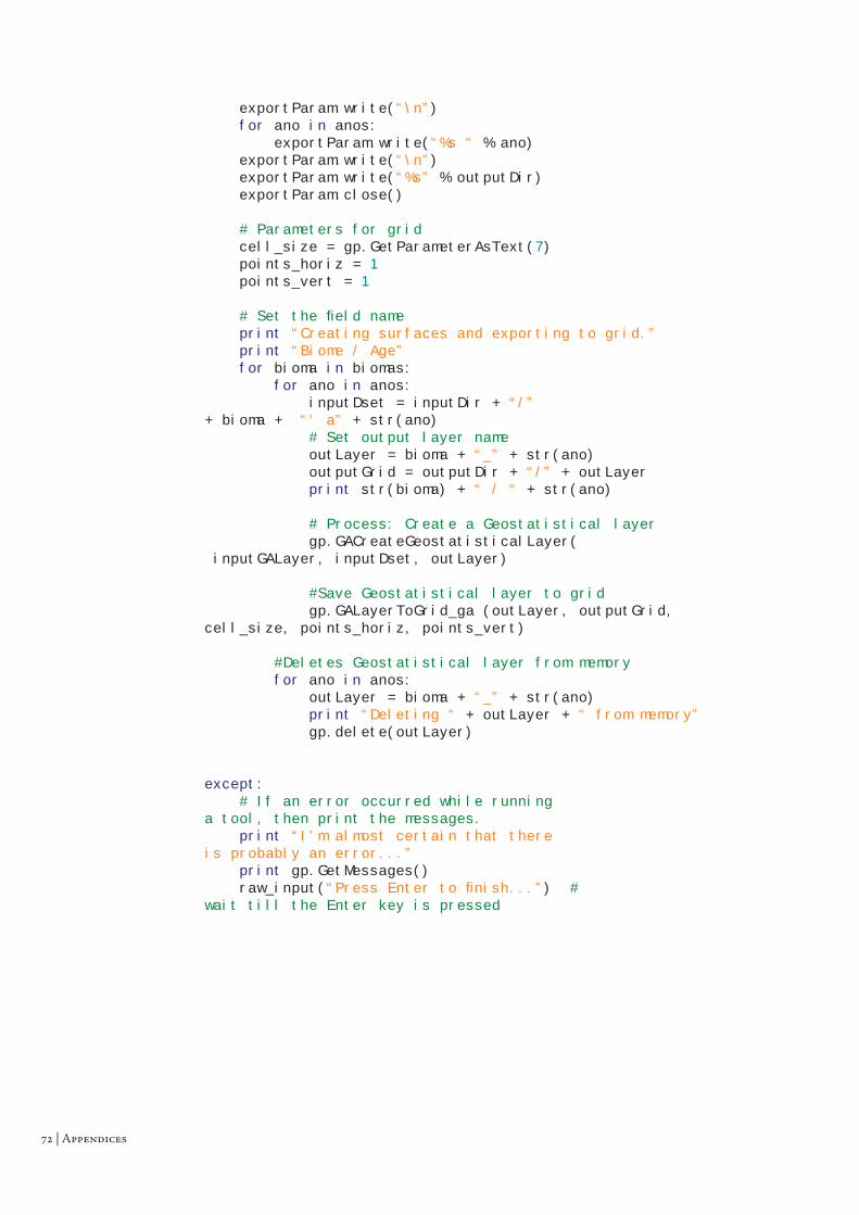
| Appendices
exportParam.write(“\n”) for ano in anos: exportParam.write(“%s “ % ano) exportParam.write(“\n”) exportParam.write(“%s” % outputDir) exportParam.close() # Parameters for grid cell_size = gp.GetParameterAsText(7) points_horiz = 1 points_vert = 1 # Set the fi eld name print “Creating surfaces and exporting to grid.” print “Biome / Age” for bioma in biomas: for ano in anos: inputDset = inputDir + “/” + bioma + “’ a” + str(ano) # Set output layer name outLayer = bioma + “_” + str(ano) outputGrid = outputDir + “/” + outLayer print str(bioma) + “ / “ + str(ano) # Process: Create a Geostatistical layer gp.GACreateGeostatisticalLayer( inputGALayer, inputDset, outLayer) #Save Geostatistical layer to grid gp.GALayerToGrid_ga (outLayer, outputGrid, cell_size, points_horiz, points_vert)
#Deletes Geostatistical layer from memory for ano in anos: outLayer = bioma + “_” + str(ano) print “Deleting “ + outLayer + “ from memory” gp.delete(outLayer)
except: # If an error occurred while running a tool, then print the messages. print “I’m almost certain that there is probably an error...” print gp.GetMessages() raw_input(“Press Enter to fi nish...”) # wait till the Enter key is pressed

Appendices |
Appendix III – Script for classify Biomes
#######################################################################Geoprocessing script to classify Biomes maps based on the maximum ##affi nity values for each cell and for every age available. Uses the ##data of Parameters.txt fi le exported by interpolated Affi nity ##surfaces. Exports a text fi le with legend #######################################################################
# Create the Geoprocessor object.import arcgisscriptinggp = arcgisscripting.create()try: # Reads parameters fi le parametersFile = open(gp.GetParameterAsText(0), “r”) contents = parametersFile.readlines() parametersFile.close() biomas = contents[0].split(“ “) biomas = biomas[0:len(biomas)-1] anos = contents[1].split(“ “) anos = anos[0:len(anos)-1] inputDir = str(contents[2]) print “Biomes available in parameters fi le:” print biomas print “\n” print “Years available in parameters fi le:” print anos print “\n” # Set other variables OutDir = gp.GetParameterAsText(1) # Writes legend.txt to identify biomes legend = open(str(OutDir) + “/legend.txt”, “w”) i = 1 legend.write(“Value - Biome”) for bioma in biomas: legend.write(“\n” + str(i) + “ - “ + str(bioma)) i = i + 2 legend.close()
Th is script was developed in Python free programming language and implemented
as a toolbox in ArcGIS 9.2 (ESRI 2006). It generates the map of the maximum
biome affi nity. It uses the interpolated affi nity scores to search, in a cell by cell basis,
the maximum affi nity value and which biome it represents.
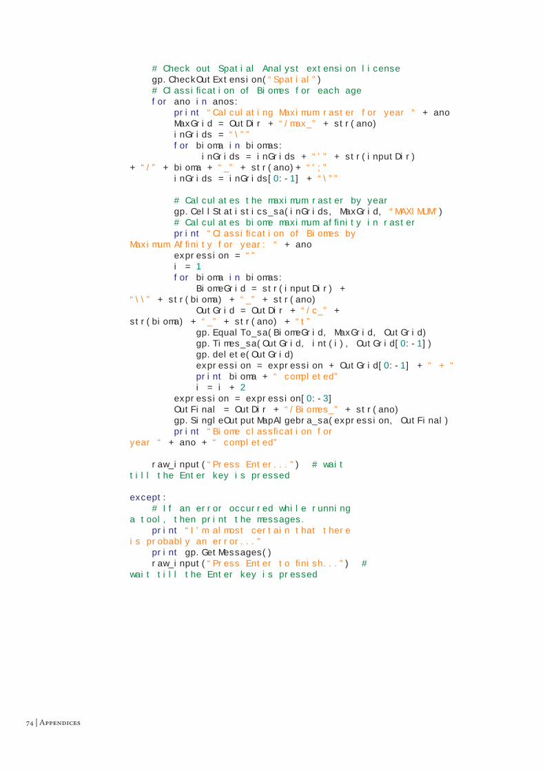
| Appendices
# Check out Spatial Analyst extension license gp.CheckOutExtension(“Spatial”) # Classifi cation of Biomes for each age for ano in anos: print “Calculating Maximum raster for year “ + ano MaxGrid = OutDir + “/max_” + str(ano) inGrids = “\”” for bioma in biomas: inGrids = inGrids + “’” + str(inputDir) + “/” + bioma + “_” + str(ano)+ “’;” inGrids = inGrids[0:-1] + “\”” # Calculates the maximum raster by year gp.CellStatistics_sa(inGrids, MaxGrid, “MAXIMUM”) # Calculates biome maximum affi nity in raster print “Classifi cation of Biomes by Maximum Affi nity for year: “ + ano expression = “” i = 1 for bioma in biomas: BiomeGrid = str(inputDir) + “\\” + str(bioma) + “_” + str(ano) OutGrid = OutDir + “/c_” + str(bioma) + “_” + str(ano) + “t” gp.EqualTo_sa(BiomeGrid, MaxGrid, OutGrid) gp.Times_sa(OutGrid, int(i), OutGrid[0:-1]) gp.delete(OutGrid) expression = expression + OutGrid[0:-1] + “ + “ print bioma + “ completed” i = i + 2 expression = expression[0:-3] OutFinal = OutDir + “/Biomes_” + str(ano) gp.SingleOutputMapAlgebra_sa(expression, OutFinal) print “Biome classfi cation for year “ + ano + “ completed” raw_input(“Press Enter...”) # wait till the Enter key is pressed except: # If an error occurred while running a tool, then print the messages. print “I’m almost certain that there is probably an error...” print gp.GetMessages() raw_input(“Press Enter to fi nish...”) # wait till the Enter key is pressed

Appendices |
Appendix IV – Script for calculating correlations between maps
from pylab import *from numpy import *
# Create the Geoprocessor object.import arcgisscriptinggp = arcgisscripting.create()
###############################################################
def read_ascii(fi lename):#Reads a ascii raster to a numpy array#Doesn’t output the header data try: myfi le = open(fi lename, “r”) contents = myfi le.readlines() myfi le.close()
#reads header and convert data to variables ncols, nrows, xllcorner, yllcorner, cellsize, nodata = int(contents[0][14:]), int(contents[1][14:]), fl oat(contents[2][14:]), fl oat(contents[3][14:]), fl oat(contents[4][14:]), fl oat(contents[5][14:])
#Create a numpy array with data MyArray = zeros([nrows-1, ncols], fl oat) i = 0 for line in contents[7:]: add(MyArray[i], [fl oat(value) for value in line.split()], MyArray[i]) i = i + 1 return MyArray except: print “Error readind ascii fi le”
###############################################################
def graphs(dataX, dataY, subplotDef, labels, **kwargs):#Creates correlation graphs#kwargs may be labely and labelx
Th is script was developed in Python free programming language and implemented as
a toolbox in ArcGIS 9.2 (ESRI 2006). It calculates the correlation value of all pair of
raster cells. Th e output is an image of correlation cloud with the general trend and
correlation value. It outputs also a text fi le with all correlations.

| Appendices
try: lim = [0,25] fontS = int((1.0000/subplotDef[0])*30)
if labels == 0: #sem labels subplot(subplotDef[0],subplotDef[1],subplotDef[2]) m, b = polyfi t(dataX,dataY,1) plot(dataX, dataY, ‘o’, dataX, m*dataX+b, ‘r’, linewidth=1, markersize =0.01) xticks(color = ‘k’, size = fontS) yticks(color = ‘k’, size = fontS)
elif labels == 1: #labels so no eixo dos X subplot(subplotDef[0],subplotDef[1],subplotDef[2]) m, b = polyfi t(dataX,dataY,1) plot(dataX, dataY, ‘o’, dataX, m*dataX+b, ‘r’, linewidth=1, markersize =0.01) xticks(color = ‘k’, size = fontS) yticks(color = ‘k’, size = fontS) xlabel(kwargs[“labely”])
elif labels == 2: #labels so no eixo dos Y subplot(subplotDef[0],subplotDef[1],subplotDef[2]) m, b = polyfi t(dataX,dataY,1) plot(dataX, dataY, ‘o’, dataX, m*dataX+b, ‘r’, linewidth=1, markersize =0.01) xticks(color = ‘k’, size = fontS) yticks(color = ‘k’, size = fontS) ylabel(kwargs[“labely”])
elif labels == 3: #labels em ambos os eixos subplot(subplotDef[0],subplotDef[1],subplotDef[2]) m, b = polyfi t(dataX,dataY,1) plot(dataX, dataY, ‘o’, dataX, m*dataX+b, ‘r’, linewidth=1, markersize =0.01) xticks(color = ‘k’, size = fontS) yticks(color = ‘k’, size = fontS) xlabel(kwargs[“labelx”]) ylabel(kwargs[“labely”])
elif labels == 4: #texto no centro sem labels subplot(subplotDef[0],subplotDef[1],subplotDef[2]) setp(gca(), xticklabels=[], yticklabels=[]) gca().text(0.5,0.5,kwargs[“textgraph”],horizontalalignment= ‘center’,verticalalignment=’center’, fontsize =8) subplots_adjust(wspace=0.4, hspace=0.4) except StandardError, e: print “Error defi ning graphs” print e
################################################################ Reads parameters fi le###############################################################
parametersFile = open(gp.GetParameterAsText(0), “r”) #Parameters fi le

Appendices |
contents = parametersFile.readlines()parametersFile.close()
biomas = contents[0].split(“ “)biomas = biomas[0:len(biomas)-1]anos = contents[1].split(“ “)anos = anos[0:len(anos)-1]#inputDir = str(contents[2])
################################################################ Set other variables###############################################################
InDir = gp.GetParameterAsText(1) #Input folderOutDir = gp.GetParameterAsText(2) #Output folder
#defi ne subplot position matrixposition = arange(power(len(biomas), 2))position = reshape(position, (len(biomas),len(biomas)))
################################################################Creates correlation graphs and matrix for each year###############################################################
try: for ano in anos: myoutfi le = open(OutDir + “\\” + ano + “_cc.txt”, “w”) myoutfi le.write(“Corelation coefi cient for year “ + ano + “\n”) for posX in range(len(biomas)): for posY in range(len(biomas)): subGraph = [len(biomas),len(biomas),(position[posY, posX] + 1)] fi leX = InDir + “\\” + biomas[posX] + “_” + ano + “.txt” coordX = ravel(read_ascii(fi leX)) fi leY = InDir + “\\” + biomas[posY] + “_” + ano + “.txt” coordY = ravel(read_ascii(fi leY)) correCoef = corrcoef(ravel(coordX), ravel(coordY)) myoutfi le.write(biomas[posX] + “ vs “ + biomas[posY] + “ = “ + str(correCoef[1][0]) + “\n”)
if posX == 0 and posY != len(biomas)-1: #na primeira coluna, excepto a ultima linha graphs(coordX, coordY, subGraph, 2, labely=biomas[posY])
elif posX == 0 and posY == len(biomas)-1: #no canto inferior esquerdo graphs(coordX, coordY, subGraph, 3, labely=biomas[posY], labelx=biomas[posX])

| Appendices
elif posX != 0 and posY == len(biomas)-1: #na ultima linha, excepto a primeira coluna graphs(coordX, coordY, subGraph, 1, labely=biomas[posX])
elif posY <= posX: graphs(coordX, coordY, subGraph, 4, textgraph=str(correCoef[1][0].round(4)))
else: graphs(coordX, coordY, subGraph, 0, labely=biomas[posY]) myoutfi le.close() savefi g(OutDir + “\\” + ano + “.svg”, dpi=300) print ano + “.svg saved!” close(‘all’) #show()
except StandardError, e: # If an error occurred while running a tool, then print the messages. print “I’m almost certain that there is probably an error...” print e raw_input(“Press Enter to fi nish...”) # wait till the Enter key is pressed
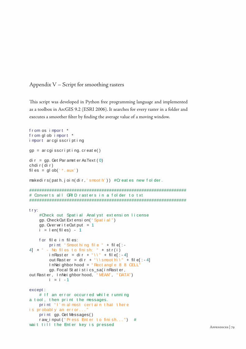
Appendices |
Appendix V – Script for smoothing rasters
from os import *from glob import *import arcgisscripting
gp = arcgisscripting.create()
dir = gp.GetParameterAsText(0)chdir(dir)fi les = glob(‘*.aux’)
makedirs(path.join(dir,’smooth’)) #Creates new folder.
################################################################ Converts all GRID rasters in a folder to txt###############################################################
try: #Check out Spatial Analyst extension license gp.CheckOutExtension(“Spatial”) gp.OverwriteOutput = 1 i = len(fi les) - 1 for fi le in fi les: print “Smoothing fi le “ + fi le[:-4] + “ - No fi les to fi nish: “ + str(i) inRaster = dir + “\\” + fi le[:-4] outRaster = dir + “\\smooth\\” + fi le[:-4] InNeighborhood = “Rectangle 8 8 CELL” gp.FocalStatistics_sa(inRaster, outRaster, InNeighborhood, “MEAN”, “DATA”) i = i -1
except: # If an error occurred while running a tool, then print the messages. print “I’m almost certain that there is probably an error...” print gp.GetMessages() raw_input(“Press Enter to fi nish...”) # wait till the Enter key is pressed
Th is script was developed in Python free programming language and implemented
as a toolbox in ArcGIS 9.2 (ESRI 2006). It searches for every raster in a folder and
executes a smoother fi lter by fi nding the average value of a moving window.

| Appendices

Appendices |
Appendix VI – Script for converting ascii fi les
from os import *from glob import *import arcgisscripting
gp = arcgisscripting.create()dir = gp.GetParameterAsText(0)chdir(dir)fi les = glob(‘*.aux’)
makedirs(path.join(dir,’txt’)) #Creates new folder.################################################################ Converts all GRID rasters in a folder to txt###############################################################
try: # Check out Spatial Analyst extension license #gp.CheckOutExtension(“Spatial”) #gp.OverwriteOutput = 1 i = len(fi les) - 1 for fi le in fi les: print “Converting fi le “ + fi le[:-4] + “ - No fi les to fi nish: “ + str(i) inRaster = dir + “\\” + fi le[:-4] outRaster = dir + “\\txt\\” + fi le[:-4] + “.txt” gp.RasterToASCII_conversion(inRaster, outRaster) i = i -1
except: # If an error occurred while running a tool, then print the messages. print “I’m almost certain that there is probably an error...” print gp.GetMessages() raw_input(“Press Enter to fi nish...”) # wait till the Enter key is pressed
Th is script was developed in Python free programming language and implemented
as a toolbox in ArcGIS 9.2 (ESRI 2006). It searches for grid maps in a folder and
converts them to ASCII fi les.

| Appendices

Appendices |
Appendix VII – Script for masking rasters
from os import *from glob import *import arcgisscripting
gp = arcgisscripting.create()
dir = gp.GetParameterAsText(0)mask = gp.GetParameterAsText(1)chdir(dir)fi les = glob(‘*.aux’)
makedirs(path.join(dir,’mask’)) #Creates new folder.
################################################################ Cuts all GRIDs in a folder by a defi ned mask###############################################################
try: #Check out Spatial Analyst extension license gp.CheckOutExtension(“Spatial”) gp.OverwriteOutput = 1 i = len(fi les) - 1 for fi le in fi les: print “Cuting grid “ + fi le[:-4] + “ - No of grids to fi nish: “ + str(i) inRaster = dir + “\\” + fi le[:-4] outRaster = dir + “\\mask\\” + fi le[:-4] gp.ExtractByMask_sa(inRaster, mask, outRaster)
i = i -1
except: # If an error occurred while running a tool, then print the messages. print “I’m almost certain that there is probably an error...” print gp.GetMessages() raw_input(“Press Enter to fi nish...”) # wait till the Enter key is pressed
Th is script was developed in Python free programming language and implemented
as a toolbox in ArcGIS 9.2 (ESRI 2006). It extracts the masked area defi ned by an
input of all rasters fi les in a folder.

| Appendices

Appendices |
Appendix VIII – Script for classifying rasters
Private Sub CopyRasterRender_Click()
Dim pMxDoc As IMxDocumentDim pMap As IMapDim pInLayer As IRasterLayerDim pOutLayer As IRasterLayer
Set pMxDoc = Application.DocumentSet pMap = pMxDoc.FocusMapSet pFromLayer = pMxDoc.SelectedLayer
Dim pId As New UIDpId = “{6CA416B1-E160-11D2-9F4E-00C04F6BC78E}” ‘datalayers
Dim pEnumLayer As IEnumLayerSet pEnumLayer = pMap.Layers(pId, True)pEnumLayer.Reset
Set pOutLayer = pEnumLayer.Next
Do While Not pOutLayer Is NothingIf TypeOf pOutLayer Is IRasterLayer Then
Set pOutLayer.Renderer = pInLayer.RendererEnd If
Set pOutLayer = pEnumLayer.NextLoop
End Sub
Th is script was developed in Visual Basic for Applications inside ArcGIS 9.2(ESRI
2006). It copies the classifi cation scheme of the selected layer to all other raster layers
in the Table of Contents.

| Appendices

Appendices |
Appendix IX – Script for exporting maps
Private Sub Ligadesliga_Click()
‘*******************************************************‘ Creates the layers list and turns on/off sequentially‘ to export all, with exception of the fi rst‘*******************************************************
Dim pDoc As IMxDocumentSet pDoc = ThisDocument
Dim pMap As IMapSet pMap = pDoc.FocusMap
Dim pLayer As IFeatureLayerDim i As LongDim NumLayer As Long
‘Export defi nitionsDim caminho As StringDim nome As StringDim tipo As StringDim dpi As IntegerDim comp As DoubleDim alt As Double
caminho = “c:\export\”tipo = “.jpg”dpi = 300comp = 4alt = 2.6
For i = 1 To pMap.LayerCount - 1pMap.Layer(i).Visible = Truenome = pMap.Layer(i).nameExporta caminho, nome, tipo, dpi, comp, altpMap.Layer(i).Visible = False
Next i
pDoc.ActiveView.Refresh
Th is script was developed in Visual Basic for Applications inside ArcGIS 9.2 (ESRI
2006). It exports all layers in the Table of Contents to an individual map with a
defi ned resolution.

| Appendices
End Sub
Public Function Exporta(caminho As String, nome As String, tipo As String, dpi As Integer, Comprimento As Double, Altura As Double)
‘**************************************************‘ Exporta o layout defi nido com a resolução‘ defi nida para um fi cheiro de imagem‘**************************************************
Dim pDoc As IMxDocumentSet pDoc = ThisDocument
Dim pActiveView As IActiveViewSet pActiveView = pDoc.ActiveView
Dim pPageLayout As IPageLayoutSet pPageLayout = pDoc.PageLayout
Dim pGC As IGraphicsContainerSet pGC = pPageLayout
Dim pGCS As IGraphicsContainerSelectDim pElement As IElementSet pElement = pGC.FindFrame(pDoc.FocusMap)
Dim pVisibleBounds As IEnvelopeSet pVisibleBounds = pElement.Geometry.Envelope
Dim pPixelBounds As IEnvelopeSet pPixelBounds = pElement.Geometry.Envelope
Dim pExport As IExport
If tipo = “.ai” ThenDim pAi As IExportAISet pAi = New ExportAISet pExport = pai
ElseIf tipo = “.emf” ThenDim pEMF As IExportEMFSet pEMF = New ExportEMFSet pExport = pEMF
ElseIf tipo = “.jpg” ThenDim pJpeg As IExportJPEGSet pJpeg = New ExportJPEGSet pExport = pJpeg
ElseIf tipo = “.pdf” ThenDim pPdf As IExportPDFSet pPdf = New ExportPDFSet pExport = pPdf
ElseIf tipo = “.tif” ThenDim pTiff As IExportTIFFSet pTiff = New ExportTIFF

Appendices |
Set pExport = pTiff
End If
Dim hDc As OLE_HANDLEDim ExportFrame As tagRECT
pExport.ExportFileName = caminho & nome & tipopExport.Resolution = dpiExportFrame.Left = 0ExportFrame.Top = 0ExportFrame.Right = Comprimento * 0.393700787 * dpiExportFrame.bottom = Altura * 0.393700787 * dpipPixelBounds.PutCoords ExportFrame.Left, ExportFrame.Top,ExportFrame.Right, ExportFrame.bottompExport.PixelBounds = pPixelBoundshDc = pExport.StartExportingpActiveView.Output hDc, pExport.Resolution, ExportFrame, pVisibleBounds,NothingpExport.FinishExporting
End Function