Large shocks in the volatility of the Dow Jones

Industrial Average index: 1928-2013

Amélie CHARLES∗

Audencia Nantes, School of Management

Olivier DARNɆ‡

LEMNA, University of Nantes

Abstract

We determine the events that cause large shocks in volatility of the DJIA in-

dex over the period 1928-2013, using a new semi-parametric test based on con-

ditional heteroscedasticity models. We find that these large shocks can be associ-

ated with particular events (financial crashes, elections, wars, monetary policies,

. . . ). We show that some shocks are not identified as extraordinary movements

by the investors due to their occurring during high volatility episodes, especially

the 1929-1934, 1937-1938 and 2007-2011 periods.

Keywords: Large shocks, Volatility, Stock market.

JEL Classification: C12; G01; N22; N42.

∗Audencia Nantes, School of Management, 8 route de la Jonelière, 44312 Nantes, France. Email:

acharles@audencia.com.†Corresponding author: LEMNA, University of Nantes, IEMN–IAE, Chemin de la Censive du Tertre,

BP 52231, 44322 Nantes, France. Tel: +33(0)2 40 14 17 05. Email: olivier.darne@univ-nantes.fr.‡Olivier Darné gratefully acknowledge financial support from the Chaire Finance of the University of

Nantes Research Foundation.

1

1 Introduction

Black Monday, as October 19, 1987, became known, was not just another

day; it was the single worst day (in percentage terms) in the Dow’s history

and therefore unique. (Estrada, 2009).

Indeed, the Dow Jones Industrial Average (DJIA) index sustained a 22.6% loss

on Black Monday. However, large daily swings that are neither unique, unusual nor

as dramatic have a substantial impact on stock market returns. Events such as wars,

terrorism, and bankruptcy are known as “black swans”.1 According to Taleb (2007),

a black swan is an event with three attributes: (i) It is an outlier, lying outside the

realm of regular expectations because nothing in the past can convincingly point to

its occurrence; (ii) it carries an extreme impact; and (iii) despite being an outlier,

plausible explanations for its occurrence can be found after the fact, thus implying

that it is explainable and predictable.

Failing to take explicit account of the fact that such extraordinary movements have

occurred in the past – and will occur in the future – is therefore a serious omission

(Friedman and Laibson, 1989). Several studies analyze the financial market reactions

to major events, by focusing on one type of event. For example, Schwert (1989b,

1990) examine the effect of the 1987 stock market crash, Frey and Kucher (2000)

and Choudhry (2010) study the impact of events during World War II, Amihud and

Wohl (2004), Rigobon and Sack (2005) and Wolfers and Zitzewitz (2009) explore

the impact of the Iraq War, Berkman, Jacobsen and Lee (2011) study the impact of

rare disasters, Schwert (1981), Flannery and Protopapadakis (2002), Bomfim (2003),

Birz and Lott (2011) and Rangel (2011) investigate macroeconomic announcements,

Akhigbe, Martin and Whyte (2005) analyze the effect of the Worldcom bankruptcy,

Chen and Siems (2004) and Chesney, Reshetar and Karaman (2011) study the

impact of terrorism, Nierderhoffer, Gibbs and Bullock (1970), Reilly and Luksetich

(1980), Foerster and Schmitz (1997), Santa-Clara and Valkanov (2003), Bialkowski,1See Taylor and Williams (2009) and Olson et al. (2012) for a discussion of “black swans” in the

money market.

2

Gottschalk and Wisniewski (2008) and Jones and Banning (2009) look at the effect

of presidential elections, and Nierderhoffer (1971) explores the impact of Presidential

illnesses. Most of these studies analyze the effects of events on financial markets where

the dates are known, most often using event study methodology.

Other studies purport to identify major shocks due to “unknown” events that affect the

stock markets before examining their implications. For example, Bloom (2009) uses

the VXO index of implied volatility (1986–2008) as a proxy for uncertainty to show

that uncertainty dramatically increases after major economic and political shocks. He

defines majors shocks as those with volatility more than 1.65 standard deviations above

the Hodrick–Prescott detrended mean of volatility. Wang et al. (2009) investigate

the causes and effects of the eight largest stock market crashes (1962–2007). They

define them as a minimum one-day decrease of 5% in the daily value-weighted market

index returns of stocks included in the Center for Research in Security Prices (CRSP)

database. Barro and Ursúa (2009) define stock-market crashes as cumulative multi-

year returns of -25% or less when studying the relation between stock-market crashes

and depressions on long-term data (1869–2006) from Global Financial Data. They

include the variables in a rare-disaster model to explain the equity premium (Barro,

2006). Cutler et al. (1989) analyze the fifty largest stock movements in the S&P

Composite Stock Index (1947–1987) which are defined as the largest one-day returns

(daily changes).

Another way to identify black swans or (infrequent) large shocks is intervention anal-

ysis, introduced by Box and Tiao (1975) to attempt to statistically appraise these types

of shocks. Intervention analysis is used to assess the impact of a known or unknown

event on the time series. The main focus is to estimate the dynamic effect of such

events on the series.2 No attempt is made here to formally define a black swan. In-

tervention analysis forms the basis for many outlier modelling procedures. A number

of procedures have been developed to identify these outliers on linear models (e.g.,

2Balke and Fomby (1994), Charles and Darné (2006), and Darné and Charles (2011) use intervention

analysis in a linear framework to identify large infrequent shocks in macroeconomic and financial times

series.

3

Tsay, 1986; Chang, Tiao and Chen, 1988; Chen and Liu, 1993). Nevertheless, it is

well known that the world is not linear, and neither are financial data. Such extreme

movements (in returns) are potentially important in finance and financial economics,

especially in modelling volatility of returns, which are an important key to risk man-

agement, derivative pricing and hedging, market making, market timing, portfolio se-

lection, monetary policy making, and many other financial activities. Several authors

consider outliers in nonlinear setting, especially from autoregressive conditionally het-

eroscedastic (ARCH) models introduced by Engle (1982) and extended to generalized

ARCH (GARCH) by Bollerslev (1986) (see, e.g., Sakata and White, 1998; Franses

and Ghijsels, 1999; Franses and van Dijk, 2000; Charles and Darné, 2005; Doornik

and Ooms, 2005; Zhang and King, 2005; Hotta and Tsay, 2012). The GARCH models,

a well-known time-varying variance specification, have been developed to capture the

two most important stylized facts of returns of financial assets, which are heavy-tailed

distribution and volatility clustering.

In this paper, the detection and identification of large shocks in volatility of the

DJIA index spanning October 2, 1928 to August 30, 2013 results from the semi-

parametric procedure to detect additive outliers proposed by Laurent, Lecourt and

Palm (LLP) (2013) based on the GJR model of Glosten, Jagannathan, and Runkle

(1993) that accounts for the so-called leverage effect.3 We determine when these

(positive and negative) large changes in volatility of daily returns occur during the

period. We use a moving subsample (10 years) window to take into account the dif-

ferent volatility levels of the DJIA in the detection of the large shocks, namely periods

with high volatility and periods with low volatility. This approach allows thus to iden-

tify large shocks as extraordinary movements perceived by the investors. The larger

changes in percentage have different consequences and perceptions when the market is

within a high volatility period compared with a low volatility period or a stable period,

3Stock returns exhibit some degree of asymmetry in their conditional variances, i.e. that market

participants overreact to bad news as compared to good news (Black, 1976; Christie, 1982; French,

Schwert and Stambaugh, 1987; Bollerslev, Chow, and Kroner, 1992).

4

especially in a context of uncertainty about the future profitability of equities and their

risk. We try to associate the date of each outlier with a specific (economic, political or

financial) event that occurred near that date, and many of them seem to be associated

with the same event patterns. We find that large shocks in volatility of the DJIA are

principally due to major financial crashes (1929, 1987, and 1997-98), US elections,

wars (e.g., Spanish Civil War, World War II, Korean war, and Gulf war), monetary

policy during recessions, macroeconomic news and declarations about the economic

situation, terrorist attacks, bankruptcy, and regulation. We also find that some negative

and positive high returns experienced by the DJIA are not identified as outliers, namely

as extraordinary (rare) movements, due to the very high volatility of some periods (see,

e.g., Officer, 1973; Schwert, 1989a). This can be explained by differing consequences

and perceptions of the investors on larger changes in percentage when the market is

within a high volatility period compared with a low volatility period or a stable period.

For example, a percentage change of −4% in returns will be not perceived in the same

way by the investors when the market is within a high or a low volatility period. This

percentage change considered as a significant shock under a low volatility regime may

become insignificant under a high volatility regime. Therefore, we use the iterative

cumulative sums of squares (ICSS) algorithm proposed by Inclán and Tiao (1994) and

improved by Sansó et al. (2004) to identify sudden shifts in volatility of the DJIA. We

find different regime changes in volatility (high, medium and low volatility), especially

episodes of high volatility occurring in 1929-1934, 1937-1938 and 2007-2011. Fur-

ther, in contrast to Schwert (2011), we show that the period of the 2007-08 financial

crisis and the related recession (2007-2011) exhibit the same characteristic than the

1929-1934 recession period: very high levels of volatility on prolonged periods (many

years).

The paper is structured as follows: Section 2 describes the methodology

identifying outliers based on a conditional heteroscedasticity model. The empirical

framework is discussed in Section 3, along with the events associated with infrequent

5

large shocks in DJIA volatility. Section 4 presents volatility changes in the DJIA. A

discussion on outliers and risk management is given in Section 5. The conclusion is

drawn in Section 6.

2 Outlier detection in GJR model

Several studies have showed that financial data may be affected by contaminated

observations (Balke and Fomby, 1994; Charles and Darné, 2005). This type of

observations, called outliers, reflects extraordinary, infrequently occurring events or

shocks that have important effects on macroeconomic and financial time series. There

are several methods for detecting outliers in nonlinear setting, such as the method for

additive jumps detection proposed by Franses and Ghijsels (1999) and Franses and van

Dijk (2000). Here we use the semi-parametric procedure to detect additive outliers

proposed by Laurent, Lecourt and Palm (LLP) (2013).4 Their test is similar to the

non-parametric tests for jumps proposed by Lee and Mykland (2008) and Andersen,

Bollerslev, and Dobrev (2007) for daily data. This method allows us to examine the

large shocks that affected the DJIA returns.

Consider the returns series rt , which is defined by rt = logPt − logPt−1, where Pt

is the observed price at time t, and consider the ARMA(p,q)-GARCH(1,1) model

ϕ(L)(rt −µ) = θ(L)εt or rt = µt + εt , (1)

εt = zt

√σ2

t ,

εt ∼ N(0,√

σ2t ), zt ∼ i.i.d.N(0,1),

σ2t = ω+α1ε2

t−1 +β1σ2t−1

where L is the lag operator, ϕ(L) = 1 − ∑pi=1 ϕiLi and θ(L) = 1 − ∑q

i=1 θiLi are

4Laurent et al. (2013) critic the sequential test for outliers proposed by Franses and Ghijsels (1999) in

two ways: (i) the critical values have to be simulated and depend on some unknown parameter values of

the GARCH model and therefore the size of the test can not be controlled; and (ii) the test suffers from

the so-called outlier masking problem because it is based on a Quasi-Maximum Likelihood estimate of

the GARCH model, which is known to be non-robust to additive outliers (Carnero et al., 2007, 2012).

They show that their test does not suffer from those drawbacks.

6

polynomials of orders p and q, respectively, such that µt = µ + ∑∞i=1 λiεt−i is the

conditional mean of rt , where λi’s are the coefficients of λ(L) = ϕ−1(L)θ(L) =

1+∑∞i=1 λiLi, and σ2

t is the conditional variance of rt .

Consider the return series with an independent additive outlier component atIt , with

outlier size at

r∗t = rt +atIt (2)

where r∗t denotes observed financial returns and It is generated by some outlier process

such as a Poisson process. The model for r∗t has the properties that an outlier atIt

will not affect σ2t+1 (the conditional variance of rt+1), and it allows for non-Gaussian

fat-tailed conditional distributions of r∗t .

Let us denote µt and σt estimates of µt and σ2t in equations (1) and (2) that are robust

to the potential presence of the additive outliers atIt (i.e. estimated on r∗t and not

on rt). The robust estimations of µt and σt are based on the bounded innovation

propagation (BIP)-ARMA proposed by Muler, Peña and Yohai (2009) and the BIP-

GARCH(1,1) proposed by Muler and Yohai (2008), respectively.The BIP-ARMA and

BIP-GARCH(1,1) are defined as

µt = µ+∞

∑i=1

λiωMPY (Jt−i) (3)

σ2t = ω+α1σ2

t−1cδωMPYkδ

(Jt−1

)2+β1σ2

t−1, (4)

where ωMPYkδ

(.) is the weight function, and cδ a factor ensuring the conditional

expectation of the weighted squared unexpected shocks to be the conditional variance

of rt in absence of jumps (Boudt et al., 2013). Laurent et al. (2013) extend the BIP-

GARCH to the BIP-GJR(1,1), i.e. the robust version of the GJR(1,1) model of Glosten,

Jagannathan, and Runkle (1993) that accounts for the so-called leverage effect, i.e.

σ2t = ω+α1σ2

t−1cδωMPYkδ

(Jt−1

)2+ γ1Dt−1σ2

t−1cδωMPYkδ

(Jt−1

)2+β1σ2

t−1, (5)

where Dt−1 = 1 if Jt−1 < 0, and 0 otherwise.

Consider the standardized return on day t

Jt =r∗t − µt

σt(6)

7

The outliers detection rule is as follow

It = I(|Jt |> k

)(7)

where I(.) is the indicator function, with It = 1 when an outlier is detected at

observation t and 0 otherwise, and k is a suitable critical value. The critical values

are defined by

k = gT,λ =− log(− log(1−λ))bT + cT , (8)

with bT = 1/√

2logT , and cT = (2logT )1/2 − [logπ + log(logT )]/[2(2logT )1/2].

They show that their test do not suffer from size distortions irrespectively of the

parameter values of the GJR model from Monte Carlo simulations. Following Laurent

et al. (2013) we set λ = 0.5. Given It , detected outliers can be filtered out from r∗t as

follows: rt = r∗t − (r∗t − µt)It .

3 Empirical study

3.1 Data description

In this section, we examine the DJIA stock market5 index spanning the October 2,

1928 to August 30, 2013, namely 21,409 observations. We consider the daily clos-

ing prices as the daily observations. Throughout the study, returns are calculated as

rt = 100× (logPt − logPt−1), with rt the log-return of each day, and Pt the index level

5The DJIA is the most-quoted market indicator in newspapers, on TV and on the Internet, and one

of most important indexes of the NYSE. Because of its longevity, it became the first to be quoted by

other publications. Besides longevity, two other factors play a role in its widespread popularity: It is

understandable to most people, and it reliably indicates the basic market trend. The DJIA is comprised

by 30 companies that are all prominent in their industries. The calculation of the DJIA is weighted price

rather than market capitalization. The component weightings are therefore affected only by changes in

the stock prices, in contrast with other indices (such as Nasdaq 100 and S&P 500), whose weightings

are affected by both changes in price and in the number of shares outstanding. Note that the DJIA can

not be considered as a benchmark of US stock market due to the fact that the DJIA incorporates a small

number of components and is based on large caps. It is more considered as a large caps index. We thank

the referee for this comment.

8

at day t. Figure 1 plots the returns of the DJIA. This approach is justified because

the thrust of the study is an investigation of market volatility. Subperiod analysis is

also appropriate because stock return data may not exhibit stationary covariance over

long periods (see Pagan and Schwert, 1990). Accordingly, in this study we consider a

10-year rolling window (about 2,500 observations).6

We apply the identification procedure of additive outliers in a GJR model for the

series of returns.7 Table 1 gives descriptive statistics for the non-adjusted and outlier-

adjusted return series. The non-adjusted returns are highly non-normal, i.e. showing

evidence of negative excess skewness and excess kurtosis. They are leptokurtic

(i.e., fat-tailed distribution). The variance of the index prices is thus principally

due to infrequent but extreme deviations. The Lagrange Multiplier test for the

presence of the ARCH effect clearly indicates that the prices show strong conditional

heteroscedasticity, which is a common feature of financial data. In other words,

there are quiet periods with small price changes and turbulent periods with large

oscillations. The outlier-adjusted returns also exhibit excess kurtosis and conditional

heteroscedasticity, although the excess kurtosis decreases dramatically. However, the

excess skewness becomes insignificant, suggesting, as shown by Carnero et al. (2001)

and Charles and Darné (2005), that outliers may cause significant skewness.

3.2 A brief history of large shocks in DJIA volatility

All detected outliers are given in Tables 1-4, by timing and t-statistics as well as

point and percent changes. A number of outliers is found in the daily DJIA – 47

outliers – during the whole period. The probability of a large shock is 0.22%, with 33

negative (70%) and 14 positive (30%) large shocks, suggesting that returns are more

affected by negative large shocks than positive large shocks. We also try to associate

the date of each outlier with a specific (economic, political or financial) event that

6We used different window’s lengths and we obtained the same results.7We also applied the Bai-Perron test for detecting structural breaks in returns but we found no break.

9

occurred near that date, presenting the outlier dates in chronological order.8 In the

following subsections, since many of the identified outliers seem to be associated

with the same event patterns we discuss the events using a classification of these

patterns: financial crises, elections, wars, monetary policy during the recessions,

macroeconomic news and declarations on the economic situation, terrorist attacks,

bankruptcy and investigation, regulation, and politico-economic conflicts.

Further, Table 7 displays the 20 largest percentage changes and losses of the DJIA

between October 1928 and June 2009. This table updates and completes the work of

Schwert (1998) who present the 25 largest daily decreases.9 The worst single day in

percentage change is October 19, 1987, at −22.61%. We also find that some negative

and positive high returns experienced by the DJIA are not identified as outliers, namely

as extraordinary (rare) movements, due to the very high volatility of some periods (see,

e.g., Officer, 1973; Schwert, 1989a). This can be explained by differing consequences

and perceptions of the investors on larger changes in percentage when the market is

within a high volatility period compared with a low volatility period or a stable period,

especially in a context of uncertainty about the future profitability of equities and their

risk. A percentage change of −4% in returns is not perceived in the same way by the

investors when the market is within a high or a low volatility period.

3.2.1 Financial crises

1929 Stock Market Crash. The crash of 1929 struck the NYSE between the October

24 and 29, 1929.10 This event marks the start of the Great Depression. On the day

of the crash on October 24, 1929 (Black Thursday), a record-breaking 13 million

8The events associated with outliers are gathered from financial newspapers. Most of them are also

found by Cutler et al. (1989) when analyzing the largest stock movements in the S&P Composite Stock

Index on the 1947–1987 period.9See also the Dow Jones website for a list of the largest daily (point and percentage) changes in the

DJIA: http://www.djaverages.com.10See, e.g., White (1990), Rappoport and White (1993), Galbraith (1997) and Bierman (1998) for a

discussion of the 1929 stock market crash. See also Shachmurove (2012) for a historical overview of

financial crisis in the US.

10

shares were traded, indicating panic. In the afternoon, five banks contributed about

$20 million each to buy stock and restore confidence in the market. However, new

accumulation of sale orders slumped on the market during the weekend, triggering a

severe fall of the DJIA (−13.47%) on October 28, 1929 (Black Monday). This fall was

broad based and did not spare securities of excellent quality (blue chip stocks). During

the meeting, a conference of the bankers was held, yet it soothed the stock market only

momentarily; investors believed thought that the banks were powerless to stop the fall.

On October 29, 1929 (Black Tuesday), the DJIA collapsed by −11.73%. This severe

fall can be explained by the fact that in the middle of the meeting, panic occurred

when the market learned of the failure of the Curb brokerage firm. The major banks

and financial giants continued their efforts to stem the fall by buying large quantities of

stocks to demonstrate their confidence in the market to the public, but their efforts were

futile. In addition, the Morgan Bank and several other establishments announced that

they would charge their customers a cover of only 25%. The wall Street Management

Committee held a meeting during which the possibility of closing the Stock Exchange

(next Saturday) was examined, but finally decided that the Saturday meeting would

take place. The Federal Bank Reserve of New York appeared determined to lower

the rate of the rediscount from 6% to 5% on Thursday. In the interim, it still reduced

the rate of acceptances by 18 %. The general feeling was slightly less pessimistic. The

investors believed that the support actions of the banks would be effective.

Wall Street began to recover from this crisis on October 30, 1929 (+12.34% for the

DJIA), nearly offsetting the fall of the previous day. This recovery is due to massive

purchases carried out by banks, investment trusts and insurance companies. The

governors of the Stock Exchange decided to close on Friday and Saturday to allow

the personnel to rest.

The President Hoover’s announcement that he would sign the Hawley-Smoot Tariff

Act on imported goods on June 16, 1930, involved the fall of the DJIA by −7.87%.

On June 22, 1931, the DJIA rose to 11.90% which can be attributed to President Her-

bert Hoover’s proposal of a one-year moratorium on $250 billion of war debt owed to

11

the US government by foreign powers. This plan was regarded as the most construc-

tive economic development in two years, and was expected to stabilize international

conditions tremendously. A strong rise occurred on October 6, 1931, driven by the

noise of the formation of a powerful banking syndicate whose the aim was to repos-

sess some assets immobilized in several large financial institutions (+14.87% for the

DJIA).

1987 Stock Market Crash. On October 19, 1987, the DJIA sustained a −22.61%

collapse (the largest one-day drop in the history of major stock market indexes from

1928 through the end of 2010), known as “Black Monday”.11 This spectacular fall can

be explained by the declarations of Treasury Secretary James Baker on the week-end,

threatening Germany, which raised its interest rates, that it would decrease the dollar

further. In this case, the Louvre Accord on the stabilization of currency values could

be called into question. Therefore, the investors feared a new fall of the dollar and

that the government did not support the dollar. The situation was worsened by the

Iran-American conflict in the Persian Gulf.

On October 21, 1987, the DJIA rose by +10.15% due to the additional decline of inter-

est rates and President Ronald Reagan’s stated intention to seek, jointly with Congress,

the means of reducing the budget deficit. For investors, this implied the shift from an

anti-inflationary policy to an anti-recession policy.

1997-1998 Asian and Russian Crises. The Asian crisis started in Thailand with the

financial collapse of the Thai baht in July 1997, and spread through the economies of

Southeast Asia. Notably, the Hong Kong Stock Exchange fell steadily (the Hang Seng

index lost 33.4% in eight days). Wall Street suffered accordingly, with a loss of 7.18%

for the DJIA on October 27, 1997. This plunge obliged the NYSE to stop quotations

temporarily; it was the first time in US history that these mechanisms, adopted after

the crash of 1987, were applied.12

11See Schwert (1989b, 1990) and Carlson (2006) for a discussion of the 1987 stock market crash.12In response to the market crisis of October 1987 the NYSE instituted circuit breakers to reduce

12

The Russian crisis (also called the “Ruble crisis”) was triggered by the Asian financial

crisis and entailed a collapse of the Russian currency (ruble) along with a default of

the short-term Russian Government Treasury Bills (the GKO). This caused the Long

Term Capital Management (LTCM) hedge fund to default on several billion dollars of

financial contracts. On August 26, 1998, the Russian Central Bank terminated ruble-

dollar trading on the MICEX (Moscow Interbank Currency Exchange). The strong

fall of the DJIA (-6.37%) on August 31, 1998, can be explained by a combination of

the deterioration of the Russian and Asian crises along with the announcement of bad

economic news, namely the declines of both firm profits and household consumption

in July (-0.2%), which confirmed the slowdown of growth in the US.

3.2.2 Elections

Presidential elections. The rise of the DJIA (+4.37%) on November 7, 1940, can

be attributed to the re-election of the President Franklin Roosevelt, who ran against

Republican Wendell Willkie. The Democrat majority to the Senate and the House of

Representatives was also preserved.

The victory of Democrat Harry Truman over Republican Thomas Dewey on November

3, 1948, caused a decline on Wall Street (-3.85% for the DJIA) because investors

expected a Republican win. The fear of reestablishment of income taxes by the

Democrats can explain the fall of the DJIA (-3.34%) on November 5, 1948.

President’s Health and Assassination. The large movements of the stock market

in September 1955, are due to the illness of President Dwight Eisenhower. The

volatility and promote investor confidence. When the DJIA loses 350 points, quotations are suspended for

half an hour. The suspension is increased to one hour if the loses are of 550 points. These measurements

are supposed to give the operators time to reflect and calm themselves during periods of high market

volatility. The SEC approved amendments to Rule 80B (Trading Halts Due to Extraordinary Market

Volatility) – effective on April 15, 1998 – which revised the halt provisions and the circuit-breaker levels.

The trigger levels for a market-wide trading halt were set at 10%, 20% and 30% of the DJIA, calculated

at the beginning of each calendar quarter, using the average closing value of the DJIA for the prior month,

thereby establishing specific point values for the quarter.

13

announcement of his heart attack prompted a plunge in the DJIA (-6.54%) on

September 26, 1955. In the following days, Wall Street responded strongly to major

news concerning the President’s health: good news on September 27, 1955 (+2.28%

for the DJIA) and bad news on October 10, 1955 (-2.92% for the DJIA).13

The assassination of President John F. Kennedy in Dallas triggered the fall of the DJIA

(-2.89%) on November 22, 1963. The governor of the NYSE closed the market 30

minutes early due to huge selling orders. The arrest of President Kennedy’s assassin

can explain the increase on Wall Street on November 26, 1963 (+4.69% for the DJIA),

coupled with along the confidence in Vice-President Lyndon Johnson.

3.2.3 Wars

Spanish Civil War. The political situation in Europe, especially the civil war in Spain

(the Nationalists marched on Barcelona and conquered Catalonia a few days later),

and the deceleration of industrial activity can explain the fall of the DJIA (-5.52%) on

January 23, 1939.

World War II. On July 26, 1934, the fear of war among some of the important

European powers due to the Austrian situation implied the collapse of Wall Street

(−6.62% for the DJIA). On October 5, 1937, the DJIA plummeted by −5.33%

due to the interpretations of the speech by President Franklin Roosevelt in Chicago

concerning the positions of the US regarding a possible international conflict. Indeed,

the Quarantine Speech given by the President Franklin Roosevelt called for an

international “quarantine of the aggressor nations” as an alternative to the political

climate of American neutrality and isolationism that was prevalent at the time. The

speech was a response to aggressive actions by Italy and Japan, and suggests the use

of economic pressure, a forceful response, but less direct than outright aggression.

After the invasion of Poland by Germany on September 1, 1939, Australia, France,

13Nierderhoffer (1971) studies the relation between Presidential illnesses and stock prices. He shows

that there is a strong and consistent stock price movement in the case of death or serious illness

of a president. Nierderhoffer finds that out of five president’s sickness from 1916 to 1964, Dwight

Eisenhower’s sickness affected securities prices the most.

14

New Zealand and United Kingdom declared war on Germany on September 3, 1939.

Therefore, on September 5, 1939, traders executed a high volume of purchases to

benefit from “war boom” prices, propelling a rise in the DJIA (+9.52%).14 The fall

of the DJIA (-4.06%) on September 17, 1939, was caused by the invasion of Poland

by the Soviet Union (under the pretext of protecting the Ukrainian and Belorussian

minorities). The successive falls of the DJIA (-2.30%, -4.93%, -6.80%, -4.78%, and

-6.78%) between May 10 to 21, 1940, are due to World War II in Europe, notably

the German offensive against France and invasion of the neutral nations of Belgium,

the Netherlands, and Luxembourg, the flight of Queen Wilhelmina of the Netherlands

and her government to London, the surrender of the Dutch army, the flight of the

Belgian government after Brussels fell to German forces and the fact that German

forces reached the English Channel. The declaration of President Franklin Roosevelt

concerning the material help accorded to the Allies prompted a rise in the DJIA

(+4.73%) on June 12, 1940.

Korean War. The falls of the DJIA on June 1950 can be explained by the Korean

War. North Korea attacked South Korea on June 25, 1950, signaling the outbreak of

the Korean War (-4.64% for the DJIA), and North Korean tanks entered Seoul on June

27, 1950 (-3.71% for the DJIA), prompting investors to fear a long war.

Gulf War. The rise of the DJIA (+4.57%) on January 17, 1991, was caused by

Gulf War I, with the launching of the operation Desert Storm, in particular with the

announcement of the success of the US air raids against Iraq.

14Choudhry (2010) investigates the potential effects of the WWII events on the movements of the DJIA

stock price index and returns volatility. Events during a war affect the equity markets in two ways: (i) it

can increase or decrease the price of shares and the returns volatility, (ii) it can alter the uncertainty of the

investors about the future profitability of the equities and their risk.

15

3.2.4 Monetary Policy during Recessions15

1969–1970 Recession. The increase in the DJIA (+3.85%) on August 16, 1971 is

due to the anti-inflationary program of the President Richard Nixon, which specifies

a series of drastic economic measures (tight monetary policy) including a wage-price

freeze, intended to lift the US out of its 1969–1970 recession.

1981–1982 Recession. The rise of the DJIA (+4.05%) on August 17, 1982, can be

explained by the interest rate decline and the debt crisis due to the announcement by

Latin American countries, especially Mexico, that they could not repay their foreign

debt. An expectation of further declines in interest rates to help the economy recover

can explain the rise of the DJIA (+4.09%) on October 6, 1982.

1991-2001 Expansion. The fall of DJIA (-2.43%) on April 02, 1994, can be explained

by the Fed’s surprise announcement that it rises US interest rates for the first time in

five years. The announcement of the surprisingly sharp rise in job numbers, suggesting

no further US interest rate cuts can explained the fall of DJIA (-3.05%) on March 09,

1996.

3.2.5 Macroeconomic News and Declarations on the Economic Situation

1938-1945 Expansion. On April 9, 1943, President Franklin Roosevelt’s anti-inflation

order governing prices and wages can explain the drop in the DJIA (-3.17%).

1946-1948 Expansion. The declines in the DJIA (-5.56%) on September 3, 1946, can

be explained by labor unrest in the maritime and trucking industries. The fall of the

DJIA (-3.89%) on April 14, 1947, can be explained by the worsening of the economic

situation and the fear of new strikes.

1961-1969 Expansion. The large movements in May and June 1962 can be explained

by the economic situation. President John F. Kennedy forced the rollback of a steel

price hike, which may explain the fall of the DJIA (-5.71%) on May 28, 1962, because

investors saw this decision as a rethinking of the principle of free enterprise.

15See Mishkin and White (2002) for a discussion of the implications for monetary policy of the stock

market crashes.

16

1982-1990 Expansion. The fall of DJIA (-3.26%) on July 07, 1986, can be explained

by a fear on the health of the US economy due to negative factors, primarily weak

corporate profits and declines in production, new orders and employment in the

industrial sector during June. The DJIA fell by 2.33% on April 14, 1988, following

the announcement of the increase in the US trade deficit in February ($13.8 billion).

3.2.6 The September 11 Terrorist Attacks

The terrorist attacks in the US on September 11, 2001 affected stock markets around

the world. The US markets remained closed for four days, whereas the European

markets decided to remain open but felt the consequences of the terrorist attacks.

The DJIA fell by “only” 7.13% when the US markets reopened on September 17,

2001. Indeed, the US stock markets were supported by the interventions of the central

banks, in particular the Fed16 and the European Central Bank, which lowered their

interest rates, and by technical provisions on the repurchases of shares by companies.

Such provisions are generally used to prevent a stock market crash. Moreover, the

authorities intervened to dissuade the banks and trust companies from lending their

securities to speculative funds, to discourage short selling transactions, which amplify

market plunges.

3.2.7 Bankruptcy

The major banks’ rejection of the plan to buy out United Airlines can explain the

considerable losses in the DJIA (-6.91%) on October 13, 1989. The crash was

apparently caused by a reaction to a news story about the break-down of a $6.75 billion

leveraged buy-out deal for United Continental Holdings (UAL) Corporation, the parent

16The Fed took steps to provide a high level of liquidity ($100 billion) through the US banking and

financial sector. The Fed policy thus calmed and stabilized the economy (Chen and Siems, 2004). On

September 14, the Fed encouraged the banks to grant appropriations to the solvent borrowers and to

modify the initial terms of the credit terms and other transactions, in particular lengthening the duration

of repayment and reorganization of debt. See Chesney et al. (2011) for a discussion of the impact of

terrorism on financial markets.

17

company of United Airlines. Wall Street (+3.40% for DJIA) rebounds the October 16,

1989, with a very high trading volume (416.29 million shares).

3.2.8 Regulation

After an eleven-day interruption due to National Banking holiday,17 the NYSE re-

opened on March 15, 1933, with a strong rise (+15.34% for the DJIA). It seems that

the measures adopted by President Franklin Roosevelt to solve the banking crisis and

to balance the budget reassured investors, especially the Emergency Banking Act or

the Glass-Steagall Act18 (law to banks from engaging in speculation). These measures

placed the market under governmental control, created restrictions on advances that

brokers could receive and obliged brokers and the members of Stock Exchange to file

daily reports on bank loans.19

3.2.9 Miscellaneous

The fall of the DJIA (-3.29%) on February 27, 2007, can be explained by the

collapse of Shanghai Stock Exchange due to the tightening of monetary policy of

the Chinese government. Further, Alan Greenspan, former Fed’s Chairman, declares

that a recession could affect the US economy. Finally, investors are concerned about

the shortcomings of high-risk loans ("subprime mortgage") granted to households

less creditworthy. The two largest mortgage agencies Freddie Mac and Fannie Mae

17On March 6, 1933, the President Franklin Roosevelt imposes the closing of all the American banks

for four days (banking holiday) which necessarily implies the closing the stock markets. For a discussion

of the National banking holiday see Wigmore (1987), Schwert (1989b) and Butkiewicz (1999), inter alia.18The Glass-Steagall Act, also called Banking Act of 1933, instituted incompatibility between trading

by deposit and investment banks; created the federal system of bank deposit insurance (the Federal

Deposit Insurance Corporation, FDIC); introduced the leveling off of the interest rates on bank deposits

(Regulation Q). The Regulation was repealed in 1980 by the Depository Institutions Deregulation and

Monetary Control Act, and the Glass-Steagall Act was abrogated on November 12, 1999, by the Financial

Services Modernization Act (or Gramm-Leach-Bliley Act). See Moshirian (2011) for a discussion of

regulations and market development.19Thereafter, the Securities and Exchange Commission (SEC) – the federal organization of regulation

and control of the financial markets – was created on June 6, 1934.

18

announced that they would tighten the criteria for this type of refinancing loans. The

US equity markets (-5.55% for DJIA) have fallen quickly in reaction to the Standard

& Poor’s decision to downgrade the US credit rating from AAA to AA+.

4 Volatility changes in the DJIA

We find that some negative and positive high returns experienced by the DJIA are

not identified as outliers, namely as extraordinary (rare) movements, due to the very

high volatility of some periods (see, e.g., Officer, 1973; Schwert, 1989a). This can be

explained by differing consequences and perceptions of the investors when the market

is experiencing high volatility rather than low volatility or stability. Therefore, we

use an appropriate methodology to identify breakpoints and sudden shifts in volatility

of the DJIA. A relatively recent approach to test for volatility shifts is the iterative

cumulative sums of squares (ICSS) algorithm proposed by Inclán and Tiao (1994) and

improves by Sansó et al. (2004). This algorithm allows the detection of multiple

breakpoints in variance and has been used extensively to identify changes in volatility

of financial time series (Fernandez, 2006; Hammoumdeh and Li, 2008; Kasman, 2009,

among others).20 Nevertheless, Rodrigues and Rubia (2011) show that the asymptotic

distribution of the ICSS test statistics varies under additive outliers. The critical

values from this distribution generally prove inadequate for the test, which finds too

many breaks.21 Therefore, using the outlier-adjusted DJIA return series, we apply the

modified ICSS algorithm to detect sudden changes in volatility.

4.1 Sudden change detection

The most popular statistical methods specifically designed to detect breaks in volatil-

ity are CUSUM-type tests. As underlined by Rodrigues and Rubia (2011), the ability

20Haugen et al. (1991) used the methodology developed by Wichern et al. (1976) for identifying

variance change points in the DJIA over the period 1897–1988.21Further, Inclán and Tiao (1994) advised that “it is advisable to complement the search for variance

changes with a procedure for outlier detection”.

19

of the CUSUM tests to identify structural changes depends of the underlying assump-

tions. Financial data display a time varying volatility pattern, known as volatility clus-

tering. Andreou and Ghysels (2002) illustrate the pervasive effect of persistent volatil-

ity on CUSUM-type tests experimentally. Their results indicate that the Kokoszka and

Leipus (2000) test is robust to conditional heteroscedasticity. Sansó et al. (2004) pro-

pose a more general test than that of Kokoszka and Leipus (2000) based on the iterative

cumulative sum of squares (ICSS) algorithm developed by Inclán and Tiao (1994).

Let ri,t = 100 × log(Pi,t/Pi,t−1), where Pi,t is the price of the index i at the time t,

so that rt is the percent return of the index i from period t − 1 to t. rt is then

assumed to be a series of independent observations from a normal distribution with

zero mean and unconditional variance σ2t for t = 1, . . . ,T . Assume that the variance

within each interval is denoted by σ2j , j = 0,1, . . . ,NT , where NT is the total number of

variance changes, and 1 < κ1 < κ2 < · · · < κNT < T are the set of breakpoints. Then

the variances over the NT intervals are defined as

σ2t =

σ20, 1 < t < κ1

σ21, κ1 < t < κ2

. . .

σ2NT, κNT < t < T

The cumulative sum of squares is used to estimate the number of variance changes and

to detect the point in time of each variance shift. The cumulative sum of the squared

observations from the beginning of the series to the kth point in time is expressed as

Ck = ∑kt=1 r2

t for k = 1, . . . ,T . To test the null hypothesis of constant unconditional

variance, the Inclán–Tiao statistic is given by:

IT = supk|√

T/2Dk| (9)

where Dk =(Ck

CT

)−( k

T

), with CT is the sum of the squared residuals from the whole

sample period. The value of k that maximizes |√

T/2Dk| is the estimate of the break

date. The ICSS algorithm systematically looks for breakpoints along the sample. If

20

there are no variance shifts over the whole sample period, Dk will oscillate around

zero. Otherwise, if there are one or more variance shifts, Dk will deviate from

zero. The asymptotic distribution of the IT statistic is given by supr |W ∗(r)|, where

W ∗(r) =W (r)− rW (1) is a Brownian bridge and W (r) is standard Brownian motion.

Finite-sample critical values can be generated by simulation.

The IT statistic is designed for i.i.d. processes, which is a very strong assumption

for financial data, in which there is evidence of conditional heteroscedasticity. Sansó et

al. (2004) show that the size distortions are important for heteroscedastic conditional

variance processes from Monte Carlo simulations. Their results thus invalidate the

practical use of this test for financial time series. To overcome this problem, Sansó et

al. (2004) propose a new test that explicitly consider the fourth moment properties

of the disturbances and the conditional heteroscedasticity.22 They propose a non-

parametric adjustment to the IT statistic that allows rt to obey a wide class of

dependent processes under the null hypothesis. Consistent with Sansó et al. (2004),

we use a non-parametric adjustment based on the Bartlett kernel, and the adjusted

statistic23 is given by:

AIT = supk|T−0.5Gk| (10)

where Gk = λ−0.5[Ck−

( kT

)CT

], λ= γ0+2∑m

l=1[1−l(m+1)−1

]γl , γl =T−1 ∑T

t=l+1(r2t −

σ2)(r2t−l − σ2), σ2 = T−1CT , and the lag truncation parameter m is selected using the

procedure in Newey and West (1994). Under general conditions, the asymptotic dis-

tribution of AIT statistic is also given by supr|W ∗(r)|, and finite-sample critical values

can be generated by simulation.

22Bacmann and Dubois (2002) show that one way to circumvent this problem is by filtering the return

series by a GARCH (1,1) model, and applying the ICSS algorithm developed by Inclán and Tiao (1994)

to the standardized residuals obtained from the estimation. Fernandez (2006) proposes an alternative

approach to testing for variance homogeneity based on wavelet analysis.23This adjusted statistic is equivalent to the non-parametric test proposed by Kokoszka and Leipus

(2000).

21

4.2 Sudden changes in the DJIA

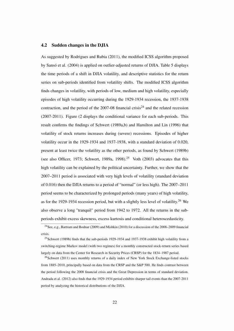
As suggested by Rodrigues and Rubia (2011), the modified ICSS algorithm proposed

by Sansó et al. (2004) is applied on outlier-adjusted returns of DJIA. Table 5 displays

the time periods of a shift in DJIA volatility, and descriptive statistics for the return

series on sub-periods identified from volatility shifts. The modified ICSS algorithm

finds changes in volatility, with periods of low, medium and high volatility, especially

episodes of high volatility occurring during the 1929-1934 recession, the 1937-1938

contraction, and the period of the 2007-08 financial crisis24 and the related recession

(2007-2011). Figure (2 displays the conditional variance for each sub-periods. This

result confirms the findings of Schwert (1989a,b) and Hamilton and Lin (1996) that

volatility of stock returns increases during (severe) recessions. Episodes of higher

volatility occur in the 1929-1934 and 1937-1938, with a standard deviation of 0.020,

present at least twice the volatility as the other periods, as found by Schwert (1989b)

(see also Officer, 1973; Schwert, 1989a, 1998).25 Voth (2003) advocates that this

high volatility can be explained by the political uncertainty. Further, we show that the

2007–2011 period is associated with very high levels of volatility (standard deviation

of 0.016) then the DJIA returns to a period of “normal” (or less high). The 2007–2011

period seems to be characterized by prolonged periods (many years) of high volatility,

as for the 1929-1934 recession period, but with a slightly less level of volatility.26 We

also observe a long "tranquil" period from 1942 to 1972. All the returns in the sub-

periods exhibit excess skewness, excess kurtosis and conditional heteroscedasticity.

24See, e.g., Bartram and Bodnar (2009) and Mishkin (2010) for a discussion of the 2008–2009 financial

crisis.25Schwert (1989b) finds that the sub-periods 1929-1934 and 1937-1938 exhibit high volatility from a

switching-regime Markov model (with two regimes) for a monthly constructed stock-return series based

largely on data from the Center for Research in Security Prices (CRSP) for the 1834–1987 period.26Schwert (2011) uses monthly returns of a daily index of New York Stock Exchange-listed stocks

from 1885–2010, principally based on data from the CRSP and the S&P 500. He finds contrast between

the period following the 2008 financial crisis and the Great Depression in terms of standard deviation.

Andrada et al. (2012) also finds that the 1929-1934 period exhibits sharper tail events than the 2007-2011

period by analyzing the historical distributions of the DJIA.

22

5 Discussion on risk management

Risk management is one of the most important innovations of the latter century. Value-

at-risk (VaR) is the most prominent of a set of risk measurement tools to be developed

in response to a series of huge, widely publicized losses at large financial firms in the

80’s.

From a statistical point of view, VaR is a quantile of the profit-loss distribution, which

can be derived for any specific level of significance (α) and time horizon.27 Financial

managers estimate the quantile of the left lower-sided tail, as a representation of worst

losses for a given (α). Providing an accurate estimate of VaR is crucial. If the underly-

ing risk is not properly estimated, this may lead to a suboptimal capital allocation with

consequences on the profitability or the financial stability of the institutions and if risk

is overestimated, then it may further lead to unnecessary extra capital requirements.

The parametric methods for estimating VaR assume one particular distribution for

the data series. The Gaussian approach implies that the returns follow a Gaussian

distribution. As it is well known that the standard deviation of the returns change over

time, we have to use models that explicitly allow the standard deviation to change of

time that provide better forecasts of variance and by extension better measures of VaR

(Engle, 2011).

Nevertheless, the presence of outliers may have undesirable effects on the estimates

of the parameters of the equation governing volatility dynamics (see, e.g., Friedman

and Laibson, 1989; Van Dijk et al., 1999; Mendes, 2000; Ng and McAleer, 2004;

Charles, 2008), the tests of conditional homoscedasticity (see, e.g., van Dijk et al.,

1999; Carnero et al., 2001, 2007), and the out-of-sample volatility forecasts (see, e.g.,

Franses and Ghijsels, 1999; Carnero et al., 2007; Catalán and Trívez, 2007; Charles,

2008).28

27VaR quantifies the potential loss for a portfolio of assets (rt ) under normal market condition over a

given period of time horizon h with a certain confidence level (1−α), at time t conditionnally on available

information Ωt−1: P(rt ≥VaRt,h(α)|Ωt−1.28Estrada (2009) show that a few outliers have a massive impact on long term performance from the

23

As one of the important steps in the estimation of VaR involves obtaining an estimate

of the volatility, we illustrate the effect of the outliers in estimating VaR. Our in-

sample period runs from October 2, 1928 to December 31, 2011, while the out-of-

sample period runs from January 02, 2013. We estimate one-day-ahead VaR from

(1) original returns, and (2) free-outlier returns, based on GJR-GARCH model29 and

daily squared returns as proxy of daily volatility.30 For comparison we use mean VaR

(VaR), the failure ratio which is the percentage of negative returns smaller than on-

step-ahead VaR, the LR Kupiec and DQ stat are the Kupiec (1995) likelihood ratio

test and the dynamic quantile (DQ) test of Engle and Manganelli (2004), respectively,

for the VaR evaluations (also known as backtests) under 95% and 99% confidence

levels. However, the VaR is not considered as a coherent measure of risk in the sense

of Artzner et al. (1999).31 Expected shortfall is a coherent measure of risk and it is

defined as the expected value of the losses conditional on the loss being larger than

the VaR.32 Hendricks (1996) indicates that two measures can be constructed: (i) the

expected value of loss exceeding the VaR level (ESF1), and (ii) the expected value

of loss exceeding the VaR level, divided by the associated VaR values (ESF2). The

results in Table 2 show that the risk measures based on outlier-free data are better than

those from original data. These results suggest that taking into account the outliers is

important for risk managers with respect to risk measure assessment, such as VaR and

expected shortfall.

We also compare the different sub-periods with some in-sample risk measures

(VaR and ES) under 95% confidence level. Table 6 displays the results and confirms

DJIA over the 1900-2006 period.29We do not search the best volatility models for computing VaR, but this point will be examined in

future research.30Our results are not sensitive to the choice of volatility proxy.31In the properties a coherent measure functional must satisfy on an appropriate probabilistic space,

the sub-additivity property does not hold for all cases. Specific portfolios can be constructed where the

risk of a portfolio with two assets can be greater than the sum of the individual risks therefore, violating

sub-additivity and in general the diversification principle (Scaillet, 2000).32The expected shortfall is defined as: ESFt = E(|Lt |> |VaRt |), where Lt is the expected value of loss

if a VaRt violation occurs.

24

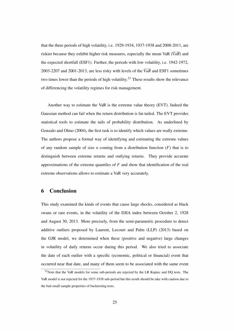
that the three periods of high volatility, i.e. 1929-1934, 1937-1938 and 2008-2011, are

riskier because they exhibit higher risk measures, especially the mean VaR (VaR) and

the expected shortfall (ESF1). Further, the periods with low volatility, i.e. 1942-1972,

2003-2207 and 2001-2013, are less risky with levels of the VaR and ESF1 sometimes

two times lower than the periods of high volatility.33 These results show the relevance

of differencing the volatility regimes for risk management.

Another way to estimate the VaR is the extreme value theory (EVT). Indeed the

Gaussian method can fail when the return distribution is fat-tailed. The EVT provides

statistical tools to estimate the tails of probability distribution. As underlined by

Gonzalo and Olmo (2004), the first task is to identify which values are really extreme.

The authors propose a formal way of identifying and estimating the extreme values

of any random sample of size n coming from a distribution function (F) that is to

distinguish between extreme returns and outlying returns. They provide accurate

approximations of the extreme quantiles of F and show that identification of the real

extreme observations allows to estimate a VaR very accurately.

6 Conclusion

This study examined the kinds of events that cause large shocks, considered as black

swans or rare events, in the volatility of the DJIA index between October 2, 1928

and August 30, 2013. More precisely, from the semi-parametric procedure to detect

additive outliers proposed by Laurent, Lecourt and Palm (LLP) (2013) based on

the GJR model, we determined when these (positive and negative) large changes

in volatility of daily returns occur during this period. We also tried to associate

the date of each outlier with a specific (economic, political or financial) event that

occurred near that date, and many of them seem to be associated with the same event

33Note that the VaR models for some sub-periods are rejected by the LR Kupiec and DQ tests. The

VaR model is not rejected for the 1937-1938 sub-period but this result should be take with caution due to

the bad small sample properties of backtesting tests.

25

patterns. We found that the large volatility shocks are principally due to the major

financial crashes, the US elections, wars, monetary policies during the recessions,

macroeconomic news and declarations on the economic situation, terrorist attacks,

bankruptcy, and regulation. This finding suggests that these large shocks should be

thus taken into account in modelling volatility of returns along with in macro-finance

models.

We also showed that some shocks were not identified as extraordinary movements due

to their occurring during high volatility episodes, especially the 1929-1934, 1937-1938

and 2007-2011 periods, identified from the ICSS algorithm. This can be explained

by differing consequences and perceptions of the investors on larger changes in

percentage when the market is within a high volatility period compared with a low

volatility period or a stable period, especially in a context of uncertainty about the

future profitability of equities and their risk. Further, in contrast to Schwert (2011),

we showed that the period of the 2007-08 financial crisis and the related recession

(2007-2011) exhibit the same characteristic than the 1929-1934 recession period: very

high levels of volatility on prolonged periods (many years). This study focuses on

the events that cause large shocks in the volatility of US stock market. It will be

interesting to study others stock markets and/or financial markets, such as bond and

foreign exchange rate markets, to compare the market’s reactions to such events.

26

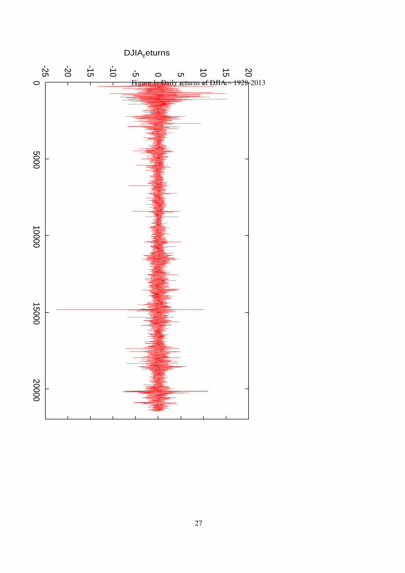
Figure 1: Daily returns of DJIA – 1928-2013

-25

-20

-15

-10 -5 0 5

10

15

20

0 5000

10000 15000

20000

DJIAreturns

27

Table 1: Summary statistics of the DJIA: 1928–2013.

Series Mean (%) St. dev. Min. Max. Skewness Excess Kurtosis LM(10)

Non-adjusted 0.0259 0.012 -0.226 0.153 -0.169∗ 20.87∗ 2738.9∗

Outlier-adjusted 0.0302 0.011 -0.107 0.114 -0.026 9.01∗ 4329.9∗

Notes: ∗ and ∗∗ mean significant at 5% and 10% level, respectively.

Table 2: Out-of-sample results for risk measures.

Series Quantile VaR Failure LR p-value DQ p-value ESF1 ESF2

ratio Kupiec Kupiec stat DQ

Non-adjusted 5% -1.212 0.044 0.382 0.537 0.366 0.545 -1.590 1.440

1% -1.716 0.025 7.213 0.007 10.27 0.001 -1.787 1.172

Outlier-adjusted 5% -1.195 0.048 0.028 0.868 0.027 0.869 -1.532 1.447

1% -1.692 0.025 7.213 0.007 10.27 0.001 -1.787 1.217

Notes: The risk measures are computed under 95% and 99% confidence levels, i.e. 5% and 1% quantiles, on the 2012-

2013 period. VaR denotes the mean on-step-ahead VaR, the failure ratio is the percentage of negative returns smaller

than on-step-ahead VaR, LR Kupiec and DQ stat are the Kupiec (1995) likelihood ratio test and the dynamic quantile

(DQ) test of Engle and Manganelli (2004), respectively, for the VaR evaluations. ESF1 and ESF2 are expected shortfall

measures defined as the expected value of loss exceeding the VaR level and the expected value of loss exceeding the

VaR level, divided by the associated VaR values, respectively.

28

Table 3: Large shocks detected in the DJIA: 1928–1948.

Point Percent

Date t-stat Change Change Events

10/28/1929 5.48 -40.58 -13.47 Black Monday

10/29/1929 4.95 -30.57 -11.73 Black Tuesday

10/30/1929 4.87 28.40 12.34 Massive purchases of stocks

06/16/1930 4.46 -19.64 -7.87 Hoover’s announcement that he would sign

the Hawley-Smoot Tariff Act

06/22/1931 5.52 15.51 11.90 Hoover debt moratorium proposal

10/06/1931 4.79 12.86 14.87 Noise of constitution of banking syndicate

03/15/1933 5.65 8.26 15.34 End of National banking holiday and Glass-Steagall Act

07/26/1934 4.34 -6.06 -6.62 Fear of European conflict

01/23/1939 5.99 -7.79 -5.22 Spanish Civil War

09/05/1939 6.68 12.87 9.52 European conflict

05/10/1940 4.27 -3.40 -2.30 World War II

05/13/1940 7.26 -7.14 -4.93 World War II

05/14/1940 8.16 -9.36 -6.80 World War II

05/17/1940 5.12 -6.23 -4.78 World War II

05/21/1940 5.54 -8.30 -6.78 World War II

11/07/1940 5.41 5.77 4.37 Roosevelt’s reelection

04/09/1943 5.71 -4.30 -3.17 Roosevelt’s anti-inflation order

09/03/1946 5.92 -10.51 -5.56 Labor unrest in maritime and trucking industries

04/14/1947 5.27 -6.74 -3.89 Worsening of economic situation

11/03/1948 6.43 -7.30 -3.85 Truman defeats Dewey

11/05/1948 4.61 -6.16 -3.34 Fear of reestablishment of earning taxes

Notes: The t-statistics are compared to the 5% critical value equal to 4.16 computed by Laurent et al. (2013).

29

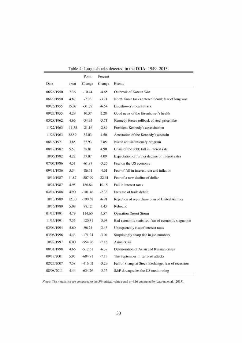
Table 4: Large shocks detected in the DJIA: 1949–2013.

Point Percent

Date t-stat Change Change Events

06/26/1950 7.36 -10.44 -4.65 Outbreak of Korean War

06/29/1950 4.87 -7.96 -3.71 North Korea tanks entered Seoul; fear of long war

09/26/1955 15.07 -31.89 -6.54 Eisenhower’s heart attack

09/27/1955 4.29 10.37 2.28 Good news of the Eisenhower’s health

05/28/1962 4.66 -34.95 -5.71 Kennedy forces rollback of steel price hike

11/22/1963 -11.38 -21.16 -2.89 President Kennedy’s assassination

11/26/1963 22.59 32.03 4.50 Arrestation of the Kennedy’s assassin

08/16/1971 3.85 32.93 3.85 Nixon anti-inflationary program

08/17/1982 5.57 38.81 4.90 Crisis of the debt; fall in interest rate

10/06/1982 4.22 37.07 4.09 Expectation of further decline of interest rates

07/07/1986 4.51 -61.87 -3.26 Fear on the US economy

09/11/1986 5.54 -86.61 -4.61 Fear of fall in interest rate and inflation

10/19/1987 11.87 -507.99 -22.61 Fear of a new decline of dollar

10/21/1987 4.95 186.84 10.15 Fall in interest rates

04/14/1988 4.90 -101.46 -2.33 Increase of trade deficit

10/13/1989 12.30 -190.58 -6.91 Rejection of repurchase plan of United Airlines

10/16/1989 5.08 88.12 3.43 Rebound

01/17/1991 4.79 114.60 4.57 Operation Desert Storm

11/15/1991 7.55 -120.31 -3.93 Bad economic statistics; fear of economic stagnation

02/04/1994 5.60 -96.24 -2.43 Unexpectedly rise of interest rates

03/08/1996 4.43 -171.24 -3.04 Surprisingly sharp rise in job numbers

10/27/1997 6.00 -554.26 -7.18 Asian crisis

08/31/1998 4.66 -512.61 -6.37 Deterioration of Asian and Russian crises

09/17/2001 5.97 -684.81 -7.13 The September 11 terrorist attacks

02/27/2007 7.58 -416.02 -3.29 Fall of Shanghai Stock Exchange; fear of recession

08/08/2011 4.44 -634.76 -5.55 S&P downgrades the US credit rating

Notes: The t-statistics are compared to the 5% critical value equal to 4.16 computed by Laurent et al. (2013).

30

Table 5: Sudden changes in DJIA volatility and summary statistics on sub-periods.

Dates of volatility Mean St. dev. Min. Max. Skewness Excess LM(10)

change breaks regimes (%) Kurtosis

10/02/1928–10/16/1934 high -0.030 0.025 -0.135 0.153 -0.354∗ 4.30∗ 157.1∗

10/17/1934–08/25/1937 medium 0.095 0.010 -0.037 0.029 -0.446∗ 1.13∗ 9.9

08/26/1937–10/05/1938 high -0.052 0.021 -0.072 0.061 -0.217∗ 0.53∗ 16.3∗∗

10/06/1938–07/08/1942 medium -0.028 0.011 -0.068 0.095 -0.031∗ 10.73∗ 48.9∗

07/09/1942–12/27/1972 low 0.032 0.007 -0.065 0.051 -0.422∗ 5.77∗ 595.6∗

12/29/1972–12/15/1995 medium 0.030 0.010 -0.226 0.101 -1.853∗ 49.53∗ 374.2∗

12/18/1995–04/02/2003 medium+ 0.033 0.012 -0.072 0.064 -0.132∗ 3.05∗ 157.8∗

04/03/2003–07/09/2007 low 0.048 0.007 -0.033 0.022 -0.088∗ 0.86∗ 31.3∗

07/10/2007–12/20/2011 high 0.002 0.016 -0.079 0.111 0.197∗ 6.90∗ 189.3∗

12/21/2011–08/30/2013 low 0.048 0.007 -0.024 0.024 -0.097∗ 1.20∗ 15.35∗

Notes: ∗ and ∗∗ mean significant at 5% and 10% level, respectively.

31

Table 6: In-sample results for risk measures on sub-periods.

Sub-periods VaR Failure LR p-value DQ p-value ESF1 ESF2

ratio Kupiec Kupiec stat DQ

10/02/1928–10/16/1934 -4.853 0.061 3.700 0.054 31.53 0.000 -4.445 1.372

10/17/1934–08/25/1937 -2.134 0.059 1.073 0.300 10.22 0.116 -1.971 1.474

08/26/1937–10/05/1938 -4.647 0.061 0.635 0.425 3.174 0.787 -4.459 1.441

10/06/1938–07/08/1942 -2.570 0.079 4.130 0.042 16.86 0.001 -2.349 1.319

07/09/1942–12/27/1972 -1.195 0.064 1.108 0.293 18.29 0.006 -1.223 1.520

12/29/1972–12/15/1995 -2.126 0.054 0.074 0.786 27.88 0.000 -2.157 1.211

12/18/1995–04/02/2003 -1.563 0.064 1.108 0.293 5.134 0.527 -1.477 1.470

04/03/2003–07/09/2007 -1.512 0.064 1.108 0.293 6.202 0.401 -1.436 1.247

07/10/2007–12/20/2011 -2.637 0.075 3.215 0.073 14.62 0.024 -2.353 1.289

12/21/2011–08/30/2013 -1.424 0.061 0.635 0.425 3.174 0.787 -1.450 1.446

Notes: The risk measures are computed under 95% confidence level. VaR denotes the mean on-step-ahead VaR, the

failure ratio is the percentage of negative returns smaller than on-step-ahead VaR, LR Kupiec and DQ stat are the

Kupiec (1995) likelihood ratio test and the dynamic quantile (DQ) test of Engle and Manganelli (2004), respectively,

for the VaR evaluations. ESF1 and ESF2 are expected shortfall measures defined as the expected value of loss

exceeding the VaR level and the expected value of loss exceeding the VaR level, divided by the associated VaR values,

respectively.

32

Figure 2: Conditional volatility of DJIA – 1928-2013

Conditional Variance

0 150 300 450 600 750 900 1050 1200 1350 1500

2.5

5.0

7.5

10.0

12.5

15.0

17.5

20.0 Conditional Variance Conditional Variance

0 100 200 300 400 500 600 700

2.5

5.0

7.5

10.0

12.5

15.0

17.5

20.0 Conditional Variance Conditional Variance

0 50 100 150 200 250

2.5

5.0

7.5

10.0

12.5

15.0

17.5

20.0 Conditional Variance

(a) 1928-1934 (b) 1934-1937 (c) 1937-1938Conditional Variance

0 50 100 150 200 250

2.5

5.0

7.5

10.0

12.5

15.0

17.5

20.0 Conditional Variance Conditional Variance

0 50 100 150 200 250

2.5

5.0

7.5

10.0

12.5

15.0

17.5

20.0 Conditional Variance Conditional Variance

0 50 100 150 200 250

2.5

5.0

7.5

10.0

12.5

15.0

17.5

20.0 Conditional Variance

(d) 1938-1942 (e) 1942-1972 (f) 1972-1995Conditional Variance

0 50 100 150 200 250

2.5

5.0

7.5

10.0

12.5

15.0

17.5

20.0 Conditional Variance Conditional Variance

0 50 100 150 200 250

2.5

5.0

7.5

10.0

12.5

15.0

17.5

20.0 Conditional Variance Conditional Variance

0 50 100 150 200 250

2.5

5.0

7.5

10.0

12.5

15.0

17.5

20.0 Conditional Variance

(g) 1995-2003 (h) 2003-2007 (i) 2007-2011Conditional Variance

0 50 100 150 200 250

2.5

5.0

7.5

10.0

12.5

15.0

17.5

20.0 Conditional Variance

(j) 2011-2013

33

Table 7: Largest daily percentage changes and losses on the DJIA, October 1928 –

December 2010.Largest changes Largest losses

Rank Date % change Date % change

1 19/10/1987 -22.61 19/10/1987 -22.61

2 15/03/1933 +15.34 28/10/1929 -12.82

3 06/10/1931 +14.87 29/10/1929 -11.73

4 28/10/1929 -12.82 10/05/1931 -10.74

5 31/10/1929 +12.34 06/11/1929 -9.92

6 29/10/1929 -11.73 12/08/1932 -8.40

7 21/09/1932 +11.36 26/10/1987 -8.04

8 13/10/2008 +11.08 15/10/2008 -7.87

9 28/10/2008 +10.88 21/07/1933 -7.84

10 10/05/1931 -10.74 01/12/2008 -7.70

10 21/10/1987 +10.15 09/10/2008 -7.33

11 06/11/1929 -9.92 18/10/1937 -7.20

12 03/08/1932 +9.52 27/10/1997 -7.18

13 11/02/1932 +9.47 05/10/1932 -7.15

14 14/11/1929 +9.36 17/09/2001 -7.13

15 18/12/1931 +9.35 24/09/1931 -7.07

16 13/02/1932 +9.19 20/07/1933 -7.07

17 06/05/1932 +9.08 29/09/2008 -6.98

18 19/04/1933 +9.03 13/10/1989 -6.91

19 08/10/1931 +8.70 08/01/1988 -6.85

34

References

[1] Akhigbe A., Martin A.D. and Whyte A.M. (2005). Contagion effects of the

world’s largest bankruptcy: The case of WorldCom. The Quaterly Review of

Economics and Finance, 45, 48-64.

[2] Amihud Y. and Wohl A. (2004). Political news and stock prices: The case of the

Saddam Hussein contracts. Journal of Banking and Finance, 28, 1185-1200.

[3] Andersen T.G., Bollerslev T. and Dobrev D. (2007): Noarbitrage semi-martingale

restrictions for continous-time volatility models subject to leverage effects, jumps

and i.i.d. noise: Theory and testable distributional implications. Journal of

Econometrics, 138, 125-180.

[4] Andrada-Félixa J., Fernández-Rodrígueza F. and Sosvilla-Rivero S. (2012).

Historical financial analogies of the current crisis. Economics Letters, 116, 190-

192.

[5] Artzner P., Delbaen F., Eber J-M. and Heath D. (1999). Coherent measures of

risk. Mathematical Finance, 9, 203-228.

[6] Bacmann J.F. and Dubois M. (2002). Volatility in emerging stock markets

revisited. European Financial Management Association, London Meeting, 26-29

June 2002.

[7] Balke N.S. and Fomby T.B. (1994). Large shocks, small shocks, and economic

fluctuations: Outliers in macroeconomic time series. Journal of Applied

Econometrics, 9, 181-200.

[8] Barro R.J. (2006). Rare disasters and asset markets in the Twentieth Century.

Quarterly Journal of Economics, 121, 823-866.

[9] Barro R.J. and Ursúa J.F. (2009). Stock-market crashes and depressions. Working

Paper No 1470, NBER.

35

[10] Bartram S.M. and Bodnar G.M. (2009). No place to hide: The global crisis in

equity markets in 2008/2009. Journal of International Money and Finance, 28,

1246-1292.

[11] Berkman H., Jacobsen B. and Lee J.B. (2011). Time-varying rare disaster risk

and stock returns. Journal of Financial Economics, 101, 313-332.

[12] Bialkowski J., Gottschalk K. and Wisniewski T.P. (2008). Stock market volatility

around national elections. Journal of Banking and Finance, 3, 1941-1953.

[13] Bierman H. (1998). The Causes of the 1929 Stock Market Crash. Greenwood

Press, Westport.

[14] Birz G. and Lott J.R. (2011). The effect of macroeconomic news on stock returns:

New evidence from newspaper coverage. Journal of Banking and Finance, 35,

2791-2800.

[15] Black F. (1976). Studies of stock price volatility change. Proceedings of the 1976

Meetings of the Business and Economics Statistics Section, American Statistical

Association, 177-181.

[16] Bloom N. (2009). The impact of uncertainty shocks. Econometrica, 77, 623-685.

[17] Bollerslev T. (1986). Generalized autoregressive conditional heteroskedasticity.

Journal of Econometrics, 31, 307-327.

[18] Bollerslev T., Chou R.Y. and Kroner K.F. (1992). ARCH modeling in finance: A

review of the theory and empirical evidence. Journal of Econometrics, 52, 5-59.

[19] Bomfim A.N. (2003). Pre-announcement effects, news effects, and volatility:

Monetary policy and the stock market. Journal of Banking and Finance, 27, 133-

151.

[20] Boudt K., Danielsson J. and Laurent S. (2013). Robust forecasting of dynamic

conditional correlation GARCH Models. International Journal of Forecasting,

29, 244-257.

36

[21] Box G.E.P. and Tiao G.C. (1975). Intervention analysis with applications to

economic and environmental problems. Journal of the American Statistical

Association, 70, 70-79.

[22] Butkiewicz J.L. (1999). The Reconstruction Finance Corporation, the gold

standard, and the banking panic of 1933. Southern Economic Journal, 66, 271-

293.

[23] Carlson M. (2006). A brief history of the 1987 stock market crash. Finance and

Economics Discussion Series No 2007-13, Federal Reserve Board.

[24] Carnero M.A., Peña D. and Ruiz E. (2001). Outliers and conditional autoregres-

sive heteroskedasticity in time series. Revista Estadistica, 53, 143-213.

[25] Carnero M.A., Peña D. and Ruiz E. (2007). Effects of outliers on the

identification and estimation of the GARCH models. Journal of Time Series

Analysis, 28, 471-497.

[26] Carnero M.A., Peña D. and Ruiz E. (2012). Estimating GARCH volatility in the

presence of outliers. Economics Letters, 114, 86-90.

[27] Catalán B. and Trívez F.J. (2007). Forecasting volatility in GARCH models with

additive outliers. Quantitative Finance, 7, 591-596.

[28] Chang I., Tiao G.C. and Chen C. (1988). Estimation of time series parameters in

the presence of outliers. Technometrics, 30, 193-204.

[29] Charles A. (2008). Forecasting volatility with outliers in GARCH models.

Journal of Forecasting, 27, 551-565.

[30] Charles A. and Darné O. (2005). Outliers and GARCH models in financial data.

Economics Letters, 86, 347-352.

[31] Charles A. and Darné O. (2006). Large shocks and the September 11th terrorist

attacks on international stock markets. Economic Modelling, 23, 683-698.

37

[32] Chen C. and Liu L.M. (1993). Joint estimation of model parameters and outlier

effects in time series. Journal of the American Statistical Association, 88, 284-

297.

[33] Chen A. and Siems T. (2004). The effects of terrorism on global capital markets.

European Journal of Political Economy, 20, 349-366.

[34] Chesney M., Reshetar G. and Karaman M. (2011). The impact of terrorism on

financial markets: An empirical study. Journal of Banking and Finance, 35, 253-

267.

[35] Choudhry T. (2010). World War II events and the Dow Jones industrial index.

Journal of Banking and Finance, 34, 1022-1031.

[36] Cutler D.M., Poterba J.M. and Summers L.H. (1989). What moves stock prices.

Journal of Portfolio Management, 15, 4-12.

[37] Darné O. and Charles A. (2011). Large shocks in U.S. macroeconomic time

series: 1860-1988. Cliometrica, 5, 79-100.

[38] Doornik J.A. and Ooms M. (2005). Outlier detection in GARCH models.

Discussion Paper No 2005-092/4, Tinbergen Institute.

[39] Engle R.F. (1982). Autoregressive conditional heteroscedasticity with estimates

of the variance of United Kingdom inflations. Econometrica, 50, 987-1007.

[40] Engle R.F. (2011). Garch 101: The use of ARCH and GARCH models in applied

econometrics. Journal of Economic Perspectives, 15, 157-168.

[41] Engle R.F. and Manganelli S. (2004). CAViaR: Conditional Autoregressive

Value-at-Risk by regression quantiles. Journal of Business and Economic

Statistics, 22, 367-381.

[42] Estrada J. (2009). Black swans, market timing, and the Dow. Applied Economics

Letters, 16, 1117-1121.

38

[43] Fernandez V. (2006). The impact of major global events on volatility shifts:

Evidence from the Asian crisis and 9/11. Economic Systems, 30, 79-97.

[44] Flannery M.J. and Protopapadakis A.A. (2002). Macroeconomic factors do

influence aggregate stock returns. Review of Financial Studies, 15, 751-782.

[45] Foerster S.R. and Schmitz J.J. (1997). The transmission of US election cycles to

international stock returns. Journal of International Business Studies, 28, 1-27.

[46] Franses P.H. and Ghijsels H. (1999). Additive outliers, GARCH and forecasting

volatility. International Journal of Forecasting, 15, 1-9.

[47] Franses P.H. and van Dijk D. (2000). Nonlinear Time Series Models in Empirical

Finance. Cambridge University Press, Cambridge.

[48] Frey B. and Kucher M. (2000). History as reflected in capital markets: The case

of World War II. Journal of Economic History, 60, 468-496.

[49] Friedman B.M. and Laibson D.I. (1989). Economic implications of extraordinary

movements in stock prices. Brookings Papers on Economic Activity, 2, 137-185.

[50] French K.R., Schwert G.W. and Stambaugh R.F. (1987). Expected stock returns

and volatility. Journal of Financial Economics, 19, 3-29.

[51] Galbraith J.K. (1997). The Great Crash of 1929, Boston: Houghton Mifflin.

[52] Gonzalo J. and Olmo J. (2004). Which extreme values are really extreme?

Journal of Financial Econometrics, 2, 349-369.

[53] Hamilton J. and Lin G. (1996). Stock market volatility and the business cycle.

Journal of Applied Econometrics, 5, 573-593.

[54] Hammoudeh S. and Li H. (2008). Sudden changes in volatility in emerging

markets: The case of Gulf Arab stocks markets. International Review of Financial

Analysis, 17, 47-63.

39

[55] Haugen R.A., Talmor E. and Torous W.N. (1991). The effect of volatility changes

on the level of stock prices and subsequent expected returns. The Journal of

Finance, 46, 985–1007.

[56] Hendricks D. (1996). Evaluation of Value-at-Risk models using historical data.

Economic Policy Review, 2, 39-70.

[57] Hotta L.K. and Tsay R.S. (2012). Outliers in GARCH processes. In Bell W.R,

Holan S.H. and McElroy T.S. (eds) Economic Time Series: Modeling and

Seasonality, 337-358, Chapman and Hall.

[58] Inclán C. and Tiao G.C. (1994). Use of cumulative sums of squares for

retrospective detection of changes of variance. Journal of the American Statistical

Association, 89, 913-923.

[59] Jones S.T. and Banning K. (2009). US elections and monthly stock market

returns. Journal of Economic and Finance, 33, 273-287.

[60] Kasman A. (2009). The impact of sudden changes on the persistence of volatility:

Evidence from the BRIC countries. Applied Economics Letters, 16, 759-764.

[61] Kokoszka P. and Leipus R. (2000). Change-point estimation in ARCH models.

Bernoulli, 6, 513-539.

[62] Kupiec P.H. (1995). Techniques for verifying the accuracy of risk measurement

models. Journal of Derivatives, 3, 73-84.

[63] Laurent S, Lecourt C. and Palm F.C. (2013). Testing for jumps in GARCH

models, a robust approach. Working paper.

[64] Lee S.S. and Mykland P.A. (2008). Jumps in financial markets: a new

nonparametric test and jump dynamics. Review of Financial studies, 21, 2535-

2563.

40

[65] Mendes B.V.M. (2000). Assessing the bias of maximum likelihood estimates

of contaminated GARCH models. Journal of Statistical Computation and

Simulation, 67, 359-76.

[66] Mishkin F.S. (2010). Over the cliff: From the subprime to the global financial

crisis. Working Paper No 16609, NBER.

[67] Mishkin F.S. and White E.N. (2002). US stock market crashes and their

aftermath: Implications for monetary policy. Working Paper No 8992, NBER.

[68] Moshirian F. (2011). The global financial crisis and the evolution of markets,

institutions and regulation. Journal of Banking and Finance, 35, 502-511.

[69] Muler N., Peña D. and Yohai V. (2009). Robust estimation for ARMA models.

The Annals of Statistics, 37, 816-840.

[70] Muler N. and Yohai V. (2008). Robust estimates for GARCH models. Journal of

Statistical Planning and Inference, 138, 2918-2940.

[71] Ng H.G. and McAleer M. (2004). Recursive modeling of symmetric volatility in

the presence of extreme observations. International Journal of Forecasting, 20,

115-129.

[72] Nierderhoffer V., Gibbs S. and Bullock J. (1970). Presidential elections and the

stock market. Financial Analysts Journal, 26, 111-113.

[73] Nierderhoffer V. (1971). The analysis of world events and stock prices. Journal

of Business, 44, 193-219.

[74] Officer R.R. (1973). The variability of the market factor of New York Stock

Exchange. Journal of Business, 46, 434-453.

[75] Olson E., Miller S. and Wohar M.E. (2012). “Black swans” before the

“black swan”: Evidence from international LIBOR-OIS spreads. Journal of

International Money and Finance, 31, 1339-1357.

41

[76] Rangel J.G. (2011). Macroeconomic news, announcements, and stock market

jump intensity dynamics. Journal of Banking and Finance, 35, 1263-1276.

[77] Rappoport P. and White E.N. (1993). Was there a bubble in the 1929 stock

market? Journal of Economic History, 53, 549-574.

[78] Reilly W.B. and Lukseitch W.A. (1980). The market prefers republicans: Myth

or reality? Journal of Financial and Quantitative Analysis, 15, 541-59.

[79] Rigobon R. and Sack B. (2005). The effects of war risk on U.S. financial markets.

Journal of Banking and Finance, 29, 1769-1789.

[80] Rodrigues P.M.M. and Rubia A. (2011). The effects of additive outliers and

measurement errors when testing for structural breaks in variance. Oxford

Bulletin of Economics and Statistics, 73, 449-468.

[81] Sakata S. and White H. (1998). High breakdown point conditional dispersion

estimation with application to S&P 500 daily returns volatility. Econometrica,

66, 529-567.

[82] Sansó, A., Aragó V. and Carrion-i-Silvestre J. (2004). Testing for changes in the

unconditional variance of financial time series. Revista de Economía Financiera,

4, 32-53.

[83] Santa-Clara P. and Valkanov R. (2003). The presidential puzzle: Political cycles

and the stock market. Journal of Finance, 58, 1841-72.

[84] Scaillet O. (2000). Nonparametric estimation and sensitivity analysis of expected

shortfall. Mathematical Finance, 14, 115-129.

[85] Schwert G.W. (1981). The adjustment of stock prices to information about

inflation. Journal of Finance, 36, 15-29.

[86] Schwert G.W. (1989a). Why does stock market volatility change over time?

Journal of Finance, 44, 1115-1153.

42

[87] Schwert G.W. (1989b). Business cycles, financial crises, and stock volatility.

Canegie-Rochester Conference Series on Public Policy, 31, 83-126.

[88] Schwert G.W. (1990). Stock volatility and the crash of 87. Review of Financial

Studies, 3, 77-102.

[89] Schwert G.W. (1998). Stock market volatility: Ten years after the crash. Working

Paper No 6381, NBER.

[90] Schwert G.W. (2011). Stock volatility during the recent financial crisis. European

Financial Management, 17, 789-805.

[91] Shachmurove Y. (2012). A historical overview of financial crises in the United

States. Global Finance Journal, 22, 217-231.

[92] Taleb N. (2007). The Black Swan. The Impact of the Highly Improbable. Random

House.

[93] Taylor J.B. and Williams J.C. (2009). A black swan in the money market.

American Economic Journal: Macroeconomics, 1, 58-83.

[94] Tsay R.S. (1986). Time series model specification in the presence of outliers.

Journal of the American Statistical Association, 81, 132-141.

[95] van Dijk D., Franses P.H. and Lucas A. (1999). Testing for ARCH in the presence

of additive outliers. Journal of Applied Econometrics, 14, 539-562.

[96] Voth H-J. (2003). Stock price volatility and political uncertainty: Evidence from

the interwar period. Working Paper No 02-09, MIT.

[97] Wang J., Meric G., Liu Z. and Meric I. (2009). Stock market crashes, firm

characteristics, and stock returns. Journal of Banking and Finance, 33, 1563-

1574.

[98] White E.W. (1990). The stock market boom and crash of 1929 revisited. Journal

of Economic Perspectives, 4, 67-83.

43

[99] Wichern D.W., Miller R.B. and Hsu D.A. (1976). Changes of variance in first-

order autoregressive time series models-With an application. Journal of the Royal

Statistical Society, Series C, 25, 248–256.

[100] Wigmore B.A. (1987). Was the Bank Holiday of 1933 caused by a run on the

dollar? Journal of Economic History, 47, 739-755.

[101] Wolfers J. and Zitzewitz E. (2009). Using markets to inform policy: The case

of the Iraq War. Economica, 76, 225-250.

[102] Zhang X. and King M. (2005). Influence in generalized autoregressive

conditional heteroscedasticity processes. Journal of Business and Economic

Statistics, 23, 118-129.

44