Embed Size (px)
Citation preview
American Economic Review 2015, 105(11): 3352–3384 http://dx.doi.org/10.1257/aer.20121236
3352
Fiscal Volatility Shocks and Economic Activity†
By Jesús Fernández-Villaverde, Pablo Guerrón-Quintana, Keith Kuester, and Juan Rubio-Ramírez*
We study how unexpected changes in uncertainty about fiscal policy affect economic activity. First, we estimate tax and spending pro-cesses for the United States with time-varying volatility to uncover evidence of time-varying volatility. Second, we estimate a VAR for the US economy using the time-varying volatility found in the previous step. Third, we feed the tax and spending processes into an otherwise standard New Keynesian model. Both in the VAR and in the model, we find that unexpected changes in fiscal volatility shocks can have a sizable adverse effect on economic activity. An endogenous increase in markups is a key mechanism. (JEL E12, E23, E32, E52, E62)
The recovery in the United States continues to be held back by a number of other headwinds, including still-tight borrowing conditions for some busi-nesses and households, and—as I will discuss in more detail shortly—the restraining effects of fiscal policy and fiscal uncertainty.
—Ben S. Bernanke1
Policymakers and business leaders alike saw the US economy between 2008 and 2014 as being buffeted by larger-than-usual uncertainty about fiscal policy. As illustrated by a number of prolonged struggles at all levels of government, there
1 Remarks before the Committee on Financial Services, US House of Representatives, July 18, 2012. http://www.federalreserve.gov/newsevents/testimony/bernanke20120717a.htm.
* Fernández-Villaverde: Department of Economics, University of Pennsylvania, 3718 Locust Walk, Philadelphia, PA 19104 (e-mail: [email protected]); Guerrón-Quintana: Research Department, Federal Reserve Bank of Philadelphia, Ten Independence Mall, Philadelphia, PA 19106 (e-mail: [email protected]); Kuester: Department of Economics, University of Bonn, Institute for Macroeconomics and Econometrics, Adenauerallee 24-42, 53113 Bonn, Germany (e-mail: [email protected]); Rubio-Ramírez: Department of Economics, Emory University, Rich Memorial Building, Room 306, Atlanta, GA 30322; Federal Reserve Bank of Atlanta; and BBVA Research (e-mail: [email protected]). We thank participants in seminars at the Atlanta Fed, Bank of Canada, Bank of Hungary, Bank of Spain, BBVA Research, Bonn University, Board of Governors, Central Bank of Chile, Columbia University, Concordia, CREI, Dallas Fed, Drexel, Georgetown, IMF, Maryland, Northwestern, Princeton, the Philadelphia Fed, and Wayne State, and conference presentations at the EFG, Midwest Macro Meetings, the Society for Computational Economics, NBER Universities Conference, SITE, and New York Fed Monetary Conference for comments and discussions, especially Rüdiger Bachmann, Nick Bloom, Eric Leeper, Jim Nason, Giovanni Ricco, and Julia Thomas. Michael Chimowitz and Behzad Kianian provided excellent research assistance. Any views expressed herein are those of the authors and do not necessarily coincide with those of the Federal Reserve Banks of Atlanta and Philadelphia or the Federal Reserve System. Juan F. Rubio-Ramírez also thanks the Institute for Economic Analysis (IAE) and the “Programa de Excelencia en Educación e Investigación” of the Bank of Spain, and the Spanish ministry of science and technology (Ref. ECO2011-30323-c03-01) for support. We also thank the NSF for financial support. The authors declare that they have no relevant or material financial interests that relate to the research described in this paper.
† Go to http://dx.doi.org/10.1257/aer.20121236 to visit the article page for additional materials and author disclosure statement(s).
3353fernÁndez-villaverde et al.: shocks and activityvol. 105 no. 11
was little consensus among policymakers about the fiscal mix and timing going forward.2 In this paper, we investigate whether this increased uncertainty about fiscal policy has a detrimental impact on economic activity (following the litera-ture, we use the term “uncertainty” as shorthand for what would more precisely be referred to as “objective uncertainty” or “risk”). We first estimate fiscal rules for capital and labor income taxes, consumption taxes, and government expenditure in the United States that allow for time-varying volatility in their innovations. We interpret the unexpected changes in the volatility of these innovations as a repre-sentation of unexpected variations in uncertainty about fiscal policy. A key feature of our specification is that we clearly distinguish between fiscal and fiscal volatility shocks. Another important characteristic of our fiscal rules is that the uncertainty is only about temporary changes in fiscal policy. This is a deliberate choice since we know from the work of Bi, Leeper, and Leith (2013) and others that uncertainty about permanent changes in policy has important effects on economic activity. Our goal is to investigate a different question: the response of the economy to an unex-pected and temporary increase in fiscal policy uncertainty.
Next, we estimate a vector autoregression (VAR) of the US economy in the tra-dition of Christiano, Eichenbaum, and Evans (2005) augmented with the fiscal vol-atility shocks that we recovered in the first step, and a measure of markups, and compute impulse response functions (IRFs) to a positive two-standard-deviations innovation to the fiscal volatility shock to the capital income tax. We include mark-ups because they are a mechanism central to our theoretical model.
In the third step, we feed the estimated fiscal rules into a New Keynesian model, variants of which have been demonstrated to capture important properties of US business cycles (Christiano, Eichenbaum, and Evans 2005). We estimate the model to match observations of the US economy and compute its IRFs by employing a third-order perturbation method. By using the estimated rules, we assume that the higher fiscal uncertainty is temporary, but that the processes for taxes, government spending, and uncertainty follow their historical behavior. Motivated by the situ-ation of the United States in the aftermath of the financial crises, we repeat the exercise under the assumption that the economy is already at the zero lower bound (ZLB) of the nominal interest rate when it is hit by the innovation.
Our main results are as follows. First, we find a considerable amount of time-varying volatility in the processes for taxes and government spending in the United States. We show that the smoothed process for fiscal volatility maps into the historical narrative evidence. Second, our estimated VAR points out that, after a pos-itive two-standard-deviations innovation to the fiscal volatility shock to the capital income tax, output, consumption, investment, hours, and the price level fall and stay low for several quarters. Third, our theoretical model replicates these observations
2 A notorious example of increased uncertainty was the October 2013 federal government shutdown. Other cases are the Tax Relief, Unemployment Insurance Reauthorization, and Job Creation Act of 2010, which was signed into law only shortly before the Bush tax cuts and the extension of federal unemployment benefits would have expired; the discussion surrounding the federal debt limit in 2011, which was followed by the US sovereign debt being downgraded by S&P; or the starkly different platforms in the 2012 presidential election. With regard to concerns by businesses, the Philadelphia Fed’s July 2010 Business Outlook Survey reported that, of those firms that saw the demand for their products fall, 52 percent cited “Increased uncertainty about future tax rates or government regulations” as one of the reasons. Fiscal uncertainty is, in recent years, repeatedly mentioned by respondents to the Fed’s Beige Book. Finally, see the indicator constructed by Baker, Bloom, and Davis (2015).
3354 THE AMERICAN ECONOMIC REVIEW NOVEMbER 2015
except that it predicts that inflation increases. But this can be fixed if, in addition, we assume that fiscal volatility shocks enter into the Taylor rule. Fourth, we explain how endogenous markups are central to the mechanism. Fifth, when the economy is at the ZLB, the effects are larger: output drops by 1.5 percent (an effect 15 times larger than when the ZLB is not active). The reason is that, at the ZLB, the real inter-est rate cannot fall to ameliorate the contractionary effect of the unexpected change in fiscal volatility shock, as happens when the economy is outside the ZLB.
Quantitatively, we explore the effects of a positive two-standard-deviations innovation to the fiscal volatility shock. While this innovation is large, it is not an extreme event. In Section I we show evidence documenting that it is likely that we have at least three or four of those events in our sample. We do not think about fiscal volatility shocks as a main source of business cycle fluctuations, but as an important element roughly every decade or so. Furthermore, the size of the innovation is in line with the volatility literature (see, for example, Bloom 2009; and Basu and Bundick 2012).
In this paper, we evaluate one possible incarnation of the notion of fiscal uncer-tainty. We estimate fiscal rules for the United States that allow for temporary and smooth changes in the standard deviation of their innovations while keeping the rest of the fiscal rules’ parameters constant. Other scenarios are possible. First, we could allow for changes in regimes in either the standard deviation of the innovations or the rest of the fiscal rules’ parameters. We believe that the former would provide results similar to the ones reported in the paper. Given the dimensionality of our problem and that we analyze temporary changes, it would be difficult to handle the latter. Bi, Leeper, and Leith (2013) study a world in which the initial level of debt is high and can be permanently consolidated through either future tax increases or spending cuts. They explore how beliefs about the distribution of future realizations of these risks affect economic activity. The main difference is that they consider permanent changes in policy, while we focus on temporary ones. Davig and Leeper (2011) estimate Markov-switching processes for a monetary rule and a (lump-sum) tax policy rule. Using a simple New Keynesian model without capital (a key element in our model), they analyze government spending shocks in different combinations of regimes (see also Davig and Leeper 2007).
To the best of our knowledge, our paper is the first attempt to characterize the dynamic consequences of unexpected changes to fiscal volatility shocks. At the same time, our work is placed in a literature that analyzes how other types of vola-tility shocks interact with aggregate variables. Examples include Basu and Bundick (2012); Bachmann and Bayer (2013); Bloom (2009); Bloom et al. (2012); Justiniano and Primiceri (2008); Nakata (2013); and Fernández-Villaverde et al. (2011). As a novelty with respect to these papers, we consider a monetary business cycle model. After circulating a draft of this paper, we were made aware of related work by Born and Pfeifer (2014), who are also concerned with similar issues. Among several dif-ferences between the two papers, an important distinction of our approach is that our modeling of the ZLB implies much bigger effects.
Our work has connections with other research agendas. First, our paper is related to the literature that assesses how fiscal uncertainty affects the economy through long-run growth risks, such as Croce, Nguyen, and Schmid (2012). Second, there are links with another strand of the literature that focuses on the (lack of) resolution
3355fernÁndez-villaverde et al.: shocks and activityvol. 105 no. 11
of longer-term fiscal uncertainty, such as Davig, Leeper, and Walker (2010). Finally, we also follow the tradition that studies the impact of uncertainty about future prices and demand on investment decisions (see Bloom 2009).
The remainder of the paper is structured as follows. Section I estimates the tax and spending processes that form the basis for our analysis. Section II reports the VAR evidence. Section III discusses the model and Section IV our numerical imple-mentation. Sections V–VIII report the main results. We close with some final com-ments. Several online appendices present further details and additional robustness analyses.
I. Fiscal Rules with Time-Varying Volatility
This section estimates fiscal rules with time-varying volatility using data on taxes, government spending, debt, and output. The estimated rules will discipline our quantitative experiments by assuming that past fiscal behavior is a guide to assessing current behavior. There are, at least, two alternatives to our approach. First is the direct use of agents’ expectations. This would avoid the problem that the timing of uncertainty that we estimate and the actual uncertainty that agents face might be different. But, to the best of our knowledge, there are no surveys that inquire about individuals’ expectations with regard to future fiscal policies (or, as in the Survey of Professional Forecasters, it is limited to short-run forecasts of government consumption). A second alternative would be to estimate a fully fledged business cycle model and to smooth out the time-varying volatility in fiscal rules. The size of the state space in that exercise makes this strategy too onerous. In online Appendix A, we compare our estimated fiscal rules with previous work in the literature.
Data.—We build a sample of average tax rates and spending of the consolidated government sector (federal, state, and local) at quarterly frequency from 1970:I to 2014:II (see online Appendix B for details). The tax data are constructed from national income and product accounts (NIPA) as in Leeper, Plante, and Traum (2010). We use average tax rates rather than marginal tax rates. The latter are employed by Barro and Sahasakul (1983). Since the tax code for income taxes is progressive, we may underestimate the extent to which these taxes are distortion-ary. If the marginal income tax rates display similar persistence and volatility as the average tax rates, we would then undermeasure the effect of fiscal volatility shocks. The update of the Barro-Sahasakul data provided by Barro and Redlick (2011) is, unfortunately, not suitable for our purposes. Table I in Barro and Redlick (2011) reports a marginal income tax rate that weights together labor and capital income taxes. For our exercise, however, we are interested in the evolution of capital income tax rates by themselves. Government spending is government consumption and gross investment, both from NIPA. The debt series is federal debt held by the public recorded in the Federal Reserve Bank of St. Louis’ FRED database. Output comes from NIPA.
The Rules.—Our fiscal rules model the evolution of four policy instruments: government spending as a share of output, g ̃ t , and tax rates on labor income,
3356 THE AMERICAN ECONOMIC REVIEW NOVEMbER 2015
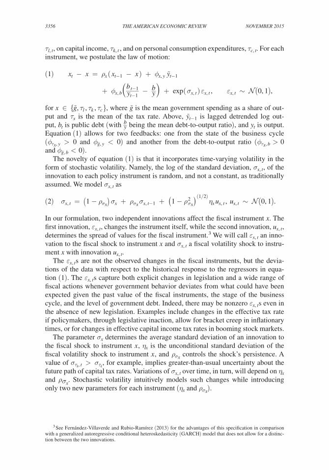
τ l, t , on capital income, τ k, t , and on personal consumption expenditures, τ c, t . For each instrument, we postulate the law of motion:
(1) x t − x = ρ x ( x t−1 − x ) + ϕ x, y y ̃ t−1
+ ϕ x, b ( b t−1 ____ y t−1 − b __ y ) + exp ( σ x, t ) ε x, t , ε x, t ∼ (0, 1) ,
for x ∈ { g ̃ , τ l , τ k , τ c } , where g ̃ is the mean government spending as a share of out-put and τ x is the mean of the tax rate. Above, y ̃ t−1 is lagged detrended log out-put, b t is public debt (with b _ y being the mean debt-to-output ratio), and y t is output. Equation (1) allows for two feedbacks: one from the state of the business cycle ( ϕ τ x , y > 0 and ϕ g ̃ , y < 0 ) and another from the debt-to-output ratio ( ϕ τ x , b > 0 and ϕ g ̃ , b < 0 ).
The novelty of equation (1) is that it incorporates time-varying volatility in the form of stochastic volatility. Namely, the log of the standard deviation, σ x, t , of the innovation to each policy instrument is random, and not a constant, as traditionally assumed. We model σ x, t as
(2) σ x, t = (1 − ρ σ x ) σ x + ρ σ x σ x, t−1 + (1 − ρ σ x 2 )
(1/2) η x u x, t , u x, t ∼ (0, 1) .
In our formulation, two independent innovations affect the fiscal instrument x . The first innovation, ε x, t , changes the instrument itself, while the second innovation, u x, t , determines the spread of values for the fiscal instrument.3 We will call ε x, t an inno-vation to the fiscal shock to instrument x and σ x, t a fiscal volatility shock to instru-ment x with innovation u x, t .
The ε x, t s are not the observed changes in the fiscal instruments, but the devia-tions of the data with respect to the historical response to the regressors in equa-tion (1). The ε x, t s capture both explicit changes in legislation and a wide range of fiscal actions whenever government behavior deviates from what could have been expected given the past value of the fiscal instruments, the stage of the business cycle, and the level of government debt. Indeed, there may be nonzero ε x, t s even in the absence of new legislation. Examples include changes in the effective tax rate if policymakers, through legislative inaction, allow for bracket creep in inflationary times, or for changes in effective capital income tax rates in booming stock markets.
The parameter σ x determines the average standard deviation of an innovation to the fiscal shock to instrument x , η x is the unconditional standard deviation of the fiscal volatility shock to instrument x , and ρ σ x controls the shock’s persistence. A value of σ τ k , t > σ τ k , for example, implies greater-than-usual uncertainty about the future path of capital tax rates. Variations of σ x, t over time, in turn, will depend on η x and ρ σ x . Stochastic volatility intuitively models such changes while introducing only two new parameters for each instrument ( η x and ρ σ x ).
3 See Fernández-Villaverde and Rubio-Ramírez (2013) for the advantages of this specification in comparison with a generalized autoregressive conditional heteroskedasticity (GARCH) model that does not allow for a distinc-tion between the two innovations.
3357fernÁndez-villaverde et al.: shocks and activityvol. 105 no. 11
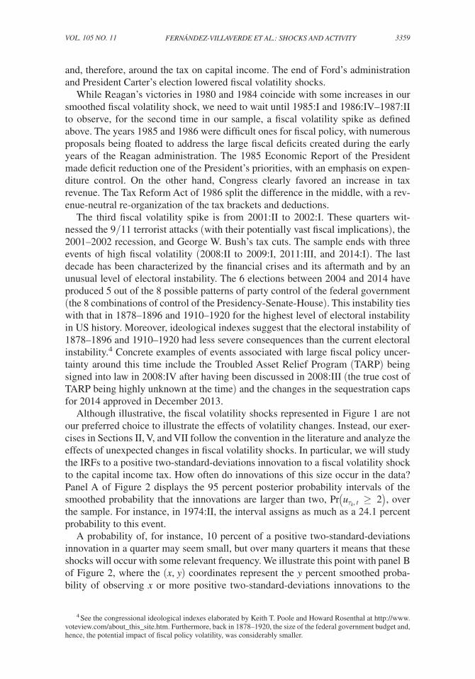
Estimation.—We estimate equations (1) and (2) for each fiscal instrument sep-arately. We set the means in equation (1) to each instrument’s average value. We estimate the rest of the parameters following a Bayesian approach by combin-ing the likelihood function with flat priors and sampling from the posterior with a Markov Chain Monte Carlo. Output is detrended with the Christiano-Fitzgerald band pass filter. The nonlinear interaction between the innovations to fiscal shocks and their volatility shocks is overcome with the particle filter as described in Fernández-Villaverde, Guerrón-Quintana, and Rubio-Ramírez (2010a) (see online Appendix C for details). Table 1 reports the posterior median for the parameters along with 95 percent probability intervals. Both tax rates and government spending as a share of output are persistent. The positive numbers in the row labeled η x pro-vide evidence that time-varying volatility is crucial. Row ρ σ x shows that, except for labor income taxes, deviations from average volatility last for some time (although that persistence is not identified as precisely as the persistence of the fiscal shocks).
Since Section V will study the effects of innovations to the fiscal volatility shocks to the capital income tax rate, u τ k , t , we focus now on the third column in Table 1. The ε τ k , t s have an average standard deviation of 0.75 percentage point ( 100 exp (−4.89) ). A positive one-standard-deviation innovation u τ k , t increases the standard deviation of the innovation to the fiscal shock to about 1 percentage point ( 100 exp (−4.89 + (1 − 0. 65 2 ) 1/2 0.40) ). The half-life of the change to the tax rate is around 34 quarters ( ρ τ k = 0.98 ).
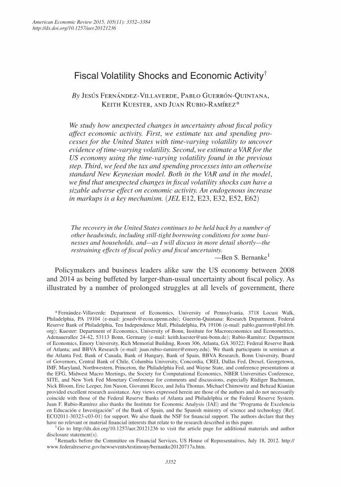
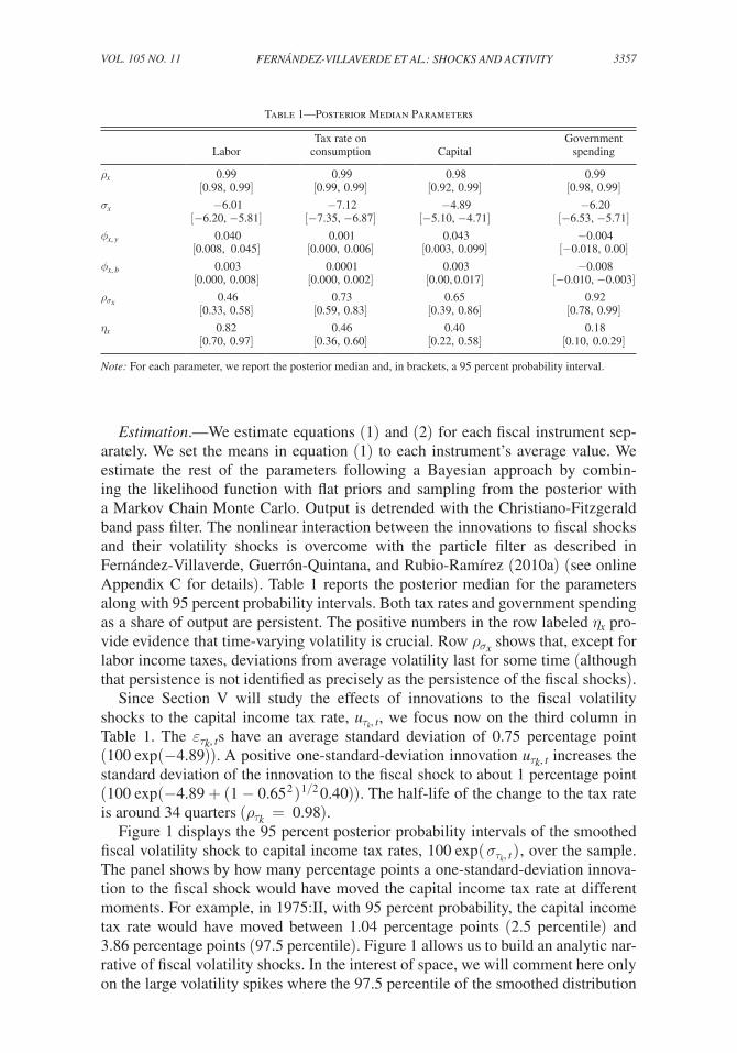
Figure 1 displays the 95 percent posterior probability intervals of the smoothed fiscal volatility shock to capital income tax rates, 100 exp ( σ τ k , t ) , over the sample. The panel shows by how many percentage points a one-standard-deviation innova-tion to the fiscal shock would have moved the capital income tax rate at different moments. For example, in 1975:II, with 95 percent probability, the capital income tax rate would have moved between 1.04 percentage points (2.5 percentile) and 3.86 percentage points (97.5 percentile). Figure 1 allows us to build an analytic nar-rative of fiscal volatility shocks. In the interest of space, we will comment here only on the large volatility spikes where the 97.5 percentile of the smoothed distribution
Table 1—Posterior Median Parameters
Tax rate on GovernmentLabor consumption Capital spending
ρ x 0.99[0.98, 0.99]
0.99[0.99, 0.99]
0.98[0.92, 0.99]
0.99[0.98, 0.99]
σ x −6.01[−6.20, −5.81]
−7.12[−7.35, −6.87]
−4.89[−5.10, −4.71]
−6.20[−6.53, −5.71]
ϕ x, y 0.040[0.008, 0.045]
0.001[0.000, 0.006]
0.043[0.003, 0.099]
−0.004[−0.018, 0.00]
ϕ x, b 0.003[0.000, 0.008]
0.0001[0.000, 0.002]
0.003[0.00, 0.017]
−0.008[−0.010, −0.003]
ρ σ x 0.46[0.33, 0.58]
0.73[0.59, 0.83]
0.65[0.39, 0.86]
0.92[0.78, 0.99]
η x 0.82[0.70, 0.97]
0.46[0.36, 0.60]
0.40[0.22, 0.58]
0.18[0.10, 0.0.29]
Note: For each parameter, we report the posterior median and, in brackets, a 95 percent probability interval.
3358 THE AMERICAN ECONOMIC REVIEW NOVEMbER 2015
of 100 exp ( σ τ k , t ) is within the 2.5 percent right tail of the unconditional distribu-tion of 100 exp ( σ τ k , t ) evaluated at the median of the posterior. Online Appendix D provides additional historical evidence and the formulae for the sets and events used to construct Figure 1.
After starting at around its historical mean, fiscal volatility climbed fast in 1974 and reached the highest point in our sample in 1975:II. The first months of 1974 wit-nessed how the Watergate scandal gathered momentum until it forced Nixon’s resig-nation on August 9, 1974. Well-informed insiders such as Arthur Burns (Chairman of the Federal Reserve Board of Governors) and George Schultz (Secretary of the Treasury until he resigned in May 1974) commented at the time on Nixon’s cavalier attitude toward economic policy and how, lost in the morass of a collapsing admin-istration, fiscal policy was drifting aimlessly, except possibly as a tool to be used to help the President survive his travails (see online Appendix D for references).
The arrival of Gerald Ford solved nothing. Ford’s staff was deeply divided about the direction that federal taxes and expenditures should follow and the President flip-flopped between increasing taxes to balance the budget and lowering them to stimulate the economy. Not only was the Congress elected in the 1974 mid-term more left-leaning than its predecessors (thus making a conflict with the Republican administration more likely), but it was also more unpredictable. In particular, the power of the Ways and Means Committee was severely damaged by the resignation of its long-time chairman Wilbur Mills, by procedural changes, by the approval of the Congressional Budget and Impoundment Control Act of 1974, and by the arrival of a cohort of new congressmen with fewer links to the traditional polit-ical machinery. As our fiscal volatility shocks indicate, 1975 was spent in bitter struggles between the President and the Congress about fiscal policy. Interestingly enough, a key part of those discussions centered around an investment tax credit
100e
xp(σ
τ k,t),
95%
pro
babi
lity
inte
rval
0
0.5
1
1.5
2
2.5
3
3.5
4
1975 1980 1985 1990 1995 2000 2005 2010
Figure 1. Smoothed Fiscal Volatility Shock to Capital Tax Rates
3359fernÁndez-villaverde et al.: shocks and activityvol. 105 no. 11
and, therefore, around the tax on capital income. The end of Ford’s administration and President Carter’s election lowered fiscal volatility shocks.
While Reagan’s victories in 1980 and 1984 coincide with some increases in our smoothed fiscal volatility shock, we need to wait until 1985:I and 1986:IV–1987:II to observe, for the second time in our sample, a fiscal volatility spike as defined above. The years 1985 and 1986 were difficult ones for fiscal policy, with numerous proposals being floated to address the large fiscal deficits created during the early years of the Reagan administration. The 1985 Economic Report of the President made deficit reduction one of the President’s priorities, with an emphasis on expen-diture control. On the other hand, Congress clearly favored an increase in tax revenue. The Tax Reform Act of 1986 split the difference in the middle, with a rev-enue-neutral re-organization of the tax brackets and deductions.
The third fiscal volatility spike is from 2001:II to 2002:I. These quarters wit-nessed the 9/11 terrorist attacks (with their potentially vast fiscal implications), the 2001–2002 recession, and George W. Bush’s tax cuts. The sample ends with three events of high fiscal volatility (2008:II to 2009:I, 2011:III, and 2014:I). The last decade has been characterized by the financial crises and its aftermath and by an unusual level of electoral instability. The 6 elections between 2004 and 2014 have produced 5 out of the 8 possible patterns of party control of the federal government (the 8 combinations of control of the Presidency-Senate-House). This instability ties with that in 1878–1896 and 1910–1920 for the highest level of electoral instability in US history. Moreover, ideological indexes suggest that the electoral instability of 1878–1896 and 1910–1920 had less severe consequences than the current electoral instability.4 Concrete examples of events associated with large fiscal policy uncer-tainty around this time include the Troubled Asset Relief Program (TARP) being signed into law in 2008:IV after having been discussed in 2008:III (the true cost of TARP being highly unknown at the time) and the changes in the sequestration caps for 2014 approved in December 2013.
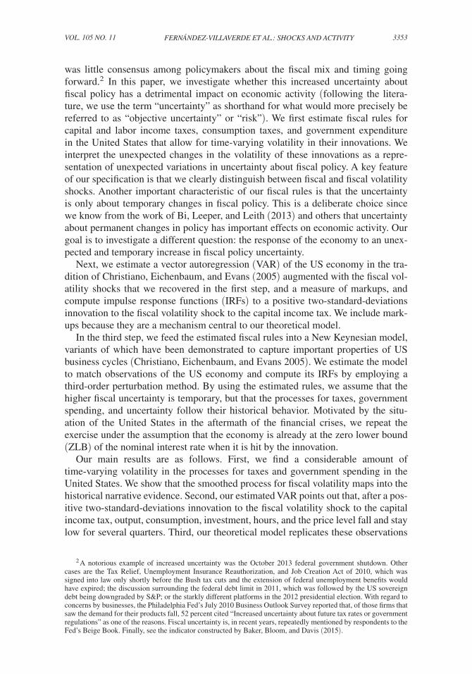
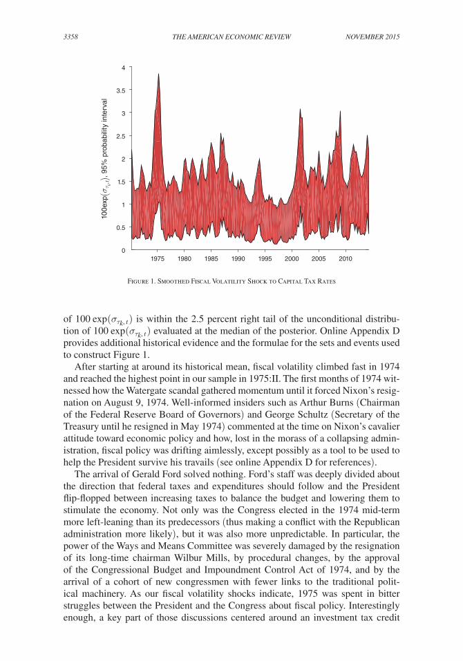
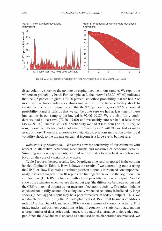
Although illustrative, the fiscal volatility shocks represented in Figure 1 are not our preferred choice to illustrate the effects of volatility changes. Instead, our exer-cises in Sections II, V, and VII follow the convention in the literature and analyze the effects of unexpected changes in fiscal volatility shocks. In particular, we will study the IRFs to a positive two-standard-deviations innovation to a fiscal volatility shock to the capital income tax. How often do innovations of this size occur in the data? Panel A of Figure 2 displays the 95 percent posterior probability intervals of the smoothed probability that the innovations are larger than two, Pr ( u τ k , t ≥ 2) , over the sample. For instance, in 1974:II, the interval assigns as much as a 24.1 percent probability to this event.
A probability of, for instance, 10 percent of a positive two-standard-deviations innovation in a quarter may seem small, but over many quarters it means that these shocks will occur with some relevant frequency. We illustrate this point with panel B of Figure 2, where the (x, y) coordinates represent the y percent smoothed proba-bility of observing x or more positive two-standard-deviations innovations to the
4 See the congressional ideological indexes elaborated by Keith T. Poole and Howard Rosenthal at http://www.voteview.com/about_this_site.htm. Furthermore, back in 1878–1920, the size of the federal government budget and, hence, the potential impact of fiscal policy volatility, was considerably smaller.
3360 THE AMERICAN ECONOMIC REVIEW NOVEMbER 2015
fiscal volatility shock to the tax rate on capital income in our sample. We report the 95 percent probability band. For example, at 2, the interval (72.20–97.60) indicates that the 2.5 percentile gives a 72.20 percent smoothed probability that we had 2 or more positive two-standard-deviations innovations to the fiscal volatility shock to capital income taxes in a quarter and that the 97.5 percentile gives a 97.60 smoothed probability. Panel B tells us that we can be quite sure we had at least one of these innovations in our sample: the interval is 92.00–99.85. We are also fairly confi-dent we had at least two (72.20–97.60) and reasonably sure we had at least three (45.44–91.60). There is still a fair probability we had at least four (22.85–77.65), or roughly one per decade, and a not small probability (2.71–40.91) we had as many as six or more. Therefore, a positive two-standard-deviations innovation to the fiscal volatility shock to the tax rate on capital income is a large event, but not rare.
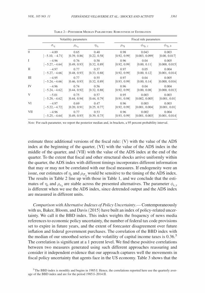
Robustness of Estimation.—We assess now the sensitivity of our estimates with respect to alternative detrending mechanisms and measures of economic activity. Summing up these experiments, we find our estimates to be robust. As before, we focus on the case of capital income taxes.
Table 2 reports the new results. Row 0 replicates the results reported in the column labeled Capital in Table 1. Row I shows the results if we detrend log output using the HP filter. Row II contains our findings when output is introduced contemporane-ously instead of lagged. Row III reports the findings when we use the log of civilian employment (CE160V) detrended with a band pass filter in lieu of output. Row IV shows the estimates when we use the output gap (the difference between output and the CBO’s potential output) as our measure of economic activity. The rules might be expected not to fully account for endogeneity when the economy is buffeted by large shocks (since lagged output may be a poor forecaster of today’s output). Thus, we reestimate our rules using the Philadelphia Fed’s ADS current business conditions index (Aruoba, Diebold, and Scotti 2009) as our measure of economic activity. This index tracks real business conditions at high frequency by statistically aggregating a large number of data series and, hence, it is a natural alternative to detrended out-put. Since the ADS index is updated as data used on its elaboration are released, we
Figure 2. Smoothed Innovations to Fiscal Volatility Shock to Capital Tax Rates
Panel B. Probability of two-standard-deviations innovations
0
5
10
15
20
25
30
01 2 3 4 5 6
10
20
30
40
50
60
70
80
90
100
1975 1980 1985 1990 1995 2000 2005 2010
≥ 2
, 95%
pro
babi
lity
inte
rval
u τk,
tPanel A. Two-standard-deviations innovations
3361fernÁndez-villaverde et al.: shocks and activityvol. 105 no. 11
estimate three additional versions of the fiscal rule: (V) with the value of the ADS index at the beginning of the quarter, (VI) with the value of the ADS index in the middle of the quarter, and (VII) with the value of the ADS index at the end of the quarter. To the extent that fiscal and other structural shocks arrive uniformly within the quarter, the ADS index with different timings incorporates different information that may or may not be correlated with our fiscal measures. If endogeneity were an issue, our estimates of η x and ρ σ x would be sensitive to the timing of the ADS index. The results in Table 2 line up with those in Table 1, and we conclude that the esti-mates of η x and ρ σ x are stable across the presented alternatives. The parameter ϕ x, y is different when we use the ADS index, since detrended output and the ADS index are measured in different units.
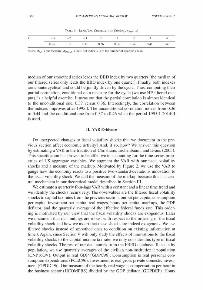
Comparison with Alternative Indexes of Policy Uncertainty.— Contemporaneously with us, Baker, Bloom, and Davis (2015) have built an index of policy-related uncer-tainty. We call it the BBD index. This index weights the frequency of news media references to economic policy uncertainty, the number of federal tax code provisions set to expire in future years, and the extent of forecaster disagreement over future inflation and federal government purchases. The correlation of the BBD index with the median of our smoothed series of the volatility of capital income taxes is 0.36.5 The correlation is significant at a 1 percent level. We find these positive correlations between two measures generated using such different approaches reassuring and consider it independent evidence that our approach captures well the movements in fiscal policy uncertainty that agents face in the US economy. Table 3 shows that the
5 The BBD index is monthly and begins in 1985:I. Hence, the correlations reported here use the quarterly aver-age of the BBD index and are for the period 1985:I–2014:II.
Table 2—Posterior Median Parameters: Robustness of Estimation
Volatility parameters Fiscal rule parameters
σ τ k ρ σ τ k η τ k ρ τ k ϕ τ k , y ϕ τ k , b
0 −4.89[−5.10, −4.71]
0.65[0.39, 0.86]
0.40[0.22, 0.58]
0.98[0.92, 0.99]
0.043[0.003, 0.099]
0.003[0.00, 0.017]
I −4.96[−5.27,−4.64]
0.76[0.49, 0.93]
0.58[0.32, 0.89]
0.96[0.92, 0.99]
0.04[0.00, 0.11]
0.005[0.000, 0.015]
II −4.97[−5.27,−4.66]
0.77[0.48, 0.93]
0.57[0.33, 0.88]
0.97[0.92, 0.99]
0.05[0.00, 0.12]
0.004[0.001, 0.014]
III −4.95[−5.24,−4.66]
0.77[0.46, 0.93]
0.55[0.32, 0.89]
0.97[0.93, 0.99]
0.04[0.00, 0.14]
0.005[0.000, 0.016]
IV −4.96[−5.24,−4.62]
0.74[0.44, 0.92]
0.56[0.32, 0.88]
0.96[0.92, 0.99]
0.04[0.00, 0.08]
0.004[0.000, 0.013]
V −5.01[−5.29,−4.62]
0.75[0.44, 0.94]
0.57[0.44, 0.79]
0.95[0.91, 0.98]
0.003[0.002, 0.005]
0.003[0.001, 0.01]
VI −4.97[−5.22,−4.72]
0.69[0.20, 0.91]
0.47[0.25, 0.77]
0.96[0.92, 0.99]
0.003[0.001, 0.004]
0.003[0.001, 0.01]
VII −4.96[−5.25,−4.64]
0.77[0.49, 0.93]
0.53[0.39, 0.75]
0.96[0.93, 0.99]
0.002[0.001, 0.003]
0.004[0.001, 0.014]
Note: For each parameter, we report the posterior median and, in brackets, a 95 percent probability interval.
3362 THE AMERICAN ECONOMIC REVIEW NOVEMbER 2015
median of our smoothed series leads the BBD index by two quarters (the median of our filtered series only leads the BBD index by one quarter). Finally, both indexes are countercyclical and could be jointly driven by the cycle. Thus, computing their partial correlation, conditional on a measure for the cycle (we use HP-filtered out-put), is a helpful exercise. It turns out that the partial correlation is almost identical to the unconditional one, 0.37 versus 0.36. Interestingly, the correlation between the indexes improves after 1995:I. The unconditional correlation moves from 0.36 to 0.44 and the conditional one from 0.37 to 0.46 when the period 1995:I–2014:II is used.
II. VAR Evidence
Do unexpected changes to fiscal volatility shocks that we document in the pre-vious section affect economic activity? And, if so, how? We answer this question by estimating a VAR in the tradition of Christiano, Eichenbaum, and Evans (2005). This specification has proven to be effective in accounting for the time-series prop-erties of US aggregate variables. We augment the VAR with our fiscal volatility shocks and a measure of the markup. Motivated by Figure 2, we use the VAR to gauge how the economy reacts to a positive two-standard-deviations innovation to the fiscal volatility shock. We add the measure of the markup because this is a cen-tral mechanism in our theoretical model described in Section III.
We estimate a quarterly four-lags VAR with a constant and a linear time trend and we identify the shocks recursively. The observables are the filtered fiscal volatility shocks to capital tax rates from the previous section, output per capita, consumption per capita, investment per capita, real wages, hours per capita, markups, the GDP deflator, and the quarterly average of the effective federal funds rate. This order-ing is motivated by our view that the fiscal volatility shocks are exogenous. Later we document that our findings are robust with respect to the ordering of the fiscal volatility shock and how we assert that these shocks are indeed exogenous. We use filtered shocks instead of smoothed ones to condition on existing information at time t . Again, since Section V will only study the effects of innovations to the fiscal volatility shocks to the capital income tax rate, we only consider this type of fiscal volatility shocks. The rest of our data comes from the FRED database. To scale by population, we use quarterly averages of the civilian non-institutional population (CNP16OV). Output is real GDP (GDPC96). Consumption is real personal con-sumption expenditures (PCEC96). Investment is real gross private domestic invest-ment (GPDIC96). Our measure of the hourly real wage is compensation per hour in the business sector (HCOMPBS) divided by the GDP deflator (GDPDEF). Hours
Table 3—Lead/Lag Correlation: Corr( σ k,t , σ BBD, t+k )
k − 3 − 2 − 1 0 1 2 3 4
0.26 0.33 0.38 0.36 0.36 0.42 0.41 0.40
Notes: σ k, t is our measure. σ BBD, t is the BBD index. k is to the number of quarters ahead.
3363fernÁndez-villaverde et al.: shocks and activityvol. 105 no. 11
per capita are measured by hours of all persons in the business sector (HOABS). The markup is measured by the inverse of the labor share in the business sector (PRS84006173). We select this measure of markup because it corresponds to the equivalent measure in our theoretical model in Section III. Inflation is based on the GDP deflator (GDPDEF). The short-term interest rate corresponds to the quarterly average of the effective federal funds rate (FEDFUNDS).
Our initial sample is from 1970:II to 2008:III. The first observation is dictated by the start of our fiscal volatility shocks. We trim the end of the sample from 2008:III to 2014:II to reserve the observations of the recent ZLB episode for an exercise where we re-estimate the VAR with those observations. Since the ZLB is a highly nonlinear event, one should be concerned about its effects in a time series linear representation such as a VAR. It is advisable, thus, to first estimate the VAR without those observations and, next, to repeat the estimation including 2008:IV to 2014:II.
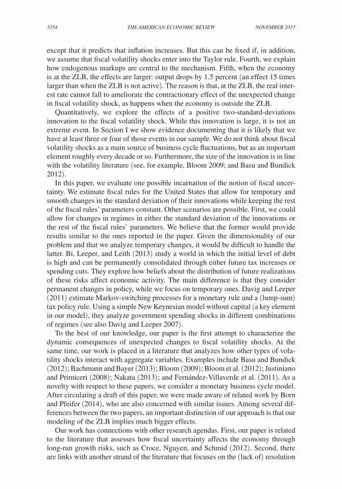
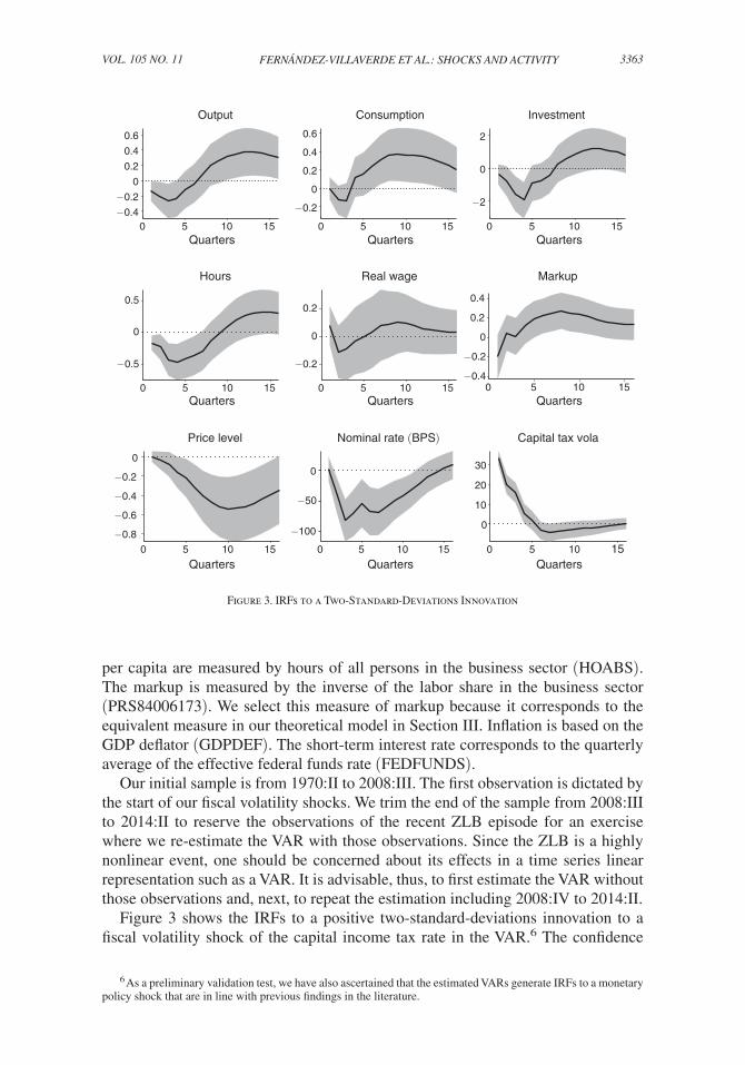
Figure 3 shows the IRFs to a positive two-standard-deviations innovation to a fiscal volatility shock of the capital income tax rate in the VAR.6 The confidence
6 As a preliminary validation test, we have also ascertained that the estimated VARs generate IRFs to a monetary policy shock that are in line with previous findings in the literature.
0 5 10 15−0.4
−0.2
0
0.2
0.4
0.6
Output
Quarters0 5 10 15
−0.2
0
0.2
0.4
0.6
Consumption
Quarters0 5 10 15
−2
0
2
Investment
Quarters
0 5 10 15
−0.5
0
0.5
Hours
0 5 10 15
−0.2
0
0.2
Real wage Markup
0 5 10 15−0.8
−0.6
−0.4
−0.2
0
Price level
0 5 10 15
−100
−50
0
Nominal rate (BPS)
0 5 10 15
0
10
20
30
Capital tax vola
Quarters Quarters Quarters
Quarters Quarters Quarters
0 5 10 15−0.4
−0.2
0
0.2
0.4
Figure 3. IRFs to a Two-Standard-Deviations Innovation
3364 THE AMERICAN ECONOMIC REVIEW NOVEMbER 2015
areas are bootstrapped, symmetric 90 percent bands. All entries are in percent, with the exception of the federal funds rate, which is in annualized basis points. Output, consumption, investment, hours, prices, the federal funds rate, and the real wage significantly fall while markups increase. This increase in markups will be a central mechanism in the theoretical model to be introduced.7
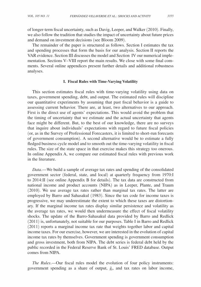
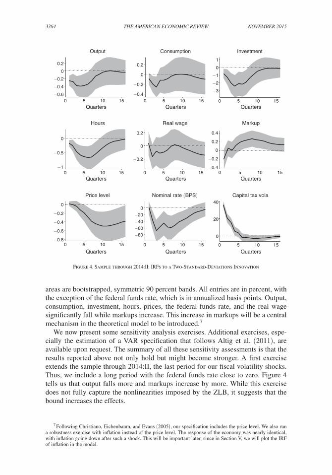
We now present some sensitivity analysis exercises. Additional exercises, espe-cially the estimation of a VAR specification that follows Altig et al. (2011), are available upon request. The summary of all these sensitivity assessments is that the results reported above not only hold but might become stronger. A first exercise extends the sample through 2014:II, the last period for our fiscal volatility shocks. Thus, we include a long period with the federal funds rate close to zero. Figure 4 tells us that output falls more and markups increase by more. While this exercise does not fully capture the nonlinearities imposed by the ZLB, it suggests that the bound increases the effects.
7 Following Christiano, Eichenbaum, and Evans (2005), our specification includes the price level. We also run a robustness exercise with inflation instead of the price level. The response of the economy was nearly identical, with inflation going down after such a shock. This will be important later, since in Section V, we will plot the IRF of inflation in the model.
Output
Quarters
Consumption
Quarters
Investment
Quarters
Hours Real wage Markup
Price level Nominal rate (BPS) Capital tax vola
Quarters Quarters Quarters
Quarters Quarters Quarters
0 5 10 15−0.6
−0.4
−0.2
0
0.2
0 5 10 15−0.4
−0.2
0
0.2
0 5 10 15
−3
−2
−1
0
1
0 5 10 15−1
−0.5
0
0 5 10 15
−0.2
0
0.2
0 5 10 15−0.8
−0.6
−0.4
−0.2
0
0 5 10 15
−80
−60
−40
−20
0
0 5 10 15
0
20
40
0 5 10 15−0.4
−0.2
0
0.2
0.4
Figure 4. Sample through 2014:II: IRFs to a Two-Standard-Deviations Innovation
3365fernÁndez-villaverde et al.: shocks and activityvol. 105 no. 11
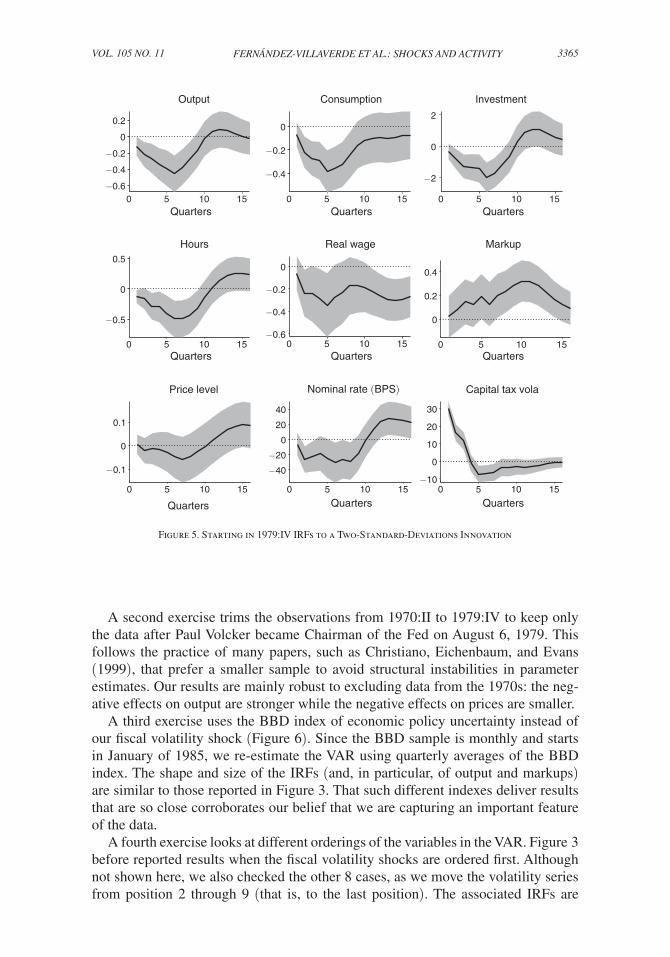
A second exercise trims the observations from 1970:II to 1979:IV to keep only the data after Paul Volcker became Chairman of the Fed on August 6, 1979. This follows the practice of many papers, such as Christiano, Eichenbaum, and Evans (1999), that prefer a smaller sample to avoid structural instabilities in parameter estimates. Our results are mainly robust to excluding data from the 1970s: the neg-ative effects on output are stronger while the negative effects on prices are smaller.
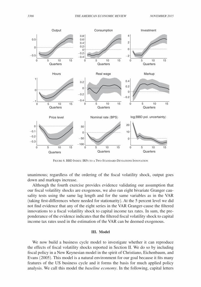
A third exercise uses the BBD index of economic policy uncertainty instead of our fiscal volatility shock (Figure 6). Since the BBD sample is monthly and starts in January of 1985, we re-estimate the VAR using quarterly averages of the BBD index. The shape and size of the IRFs (and, in particular, of output and markups) are similar to those reported in Figure 3. That such different indexes deliver results that are so close corroborates our belief that we are capturing an important feature of the data.
A fourth exercise looks at different orderings of the variables in the VAR. Figure 3 before reported results when the fiscal volatility shocks are ordered first. Although not shown here, we also checked the other 8 cases, as we move the volatility series from position 2 through 9 (that is, to the last position). The associated IRFs are
0 5 10 15−0.6
−0.4
−0.2
0
0.2
0 5 10 15
−0.4
−0.2
0
0 5 10 15
−2
0
2
0 5 10 15
−0.5
0
0.5
0 5 10 15−0.6
−0.4
−0.2
0
0 5 10 15
0
0.2
0.4
0 5 10 15
−0.1
0
0.1
0 5 10 15
−40
−20
0
20
40
0 5 10 15−10
0
10
20
30
Output Consumption Investment
Hours Real wage
Price level Nominal rate (BPS) Capital tax vola
Markup
Quarters Quarters Quarters
Quarters Quarters Quarters
Quarters Quarters Quarters
Figure 5. Starting in 1979:IV IRFs to a Two-Standard-Deviations Innovation
3366 THE AMERICAN ECONOMIC REVIEW NOVEMbER 2015
unanimous; regardless of the ordering of the fiscal volatility shock, output goes down and markups increase.
Although the fourth exercise provides evidence validating our assumption that our fiscal volatility shocks are exogenous, we also ran eight bivariate Granger cau-sality tests using the same lag length and for the same variables as in the VAR ( taking first-differences where needed for stationarity). At the 5 percent level we did not find evidence that any of the eight series in the VAR Granger-cause the filtered innovations to a fiscal volatility shock to capital income tax rates. In sum, the pre-ponderance of the evidence indicates that the filtered fiscal volatility shock to capital income tax rates used in the estimation of the VAR can be deemed exogenous.
III. Model
We now build a business cycle model to investigate whether it can reproduce the effects of fiscal volatility shocks reported in Section II. We do so by including fiscal policy in a New Keynesian model in the spirit of Christiano, Eichenbaum, and Evans (2005). This model is a natural environment for our goal because it fits many features of the US business cycle and it forms the basis for much applied policy analysis. We call this model the baseline economy. In the following, capital letters
0 5 10 15
−0.5
0
0.5
0 5 10 15−0.4−0.2
00.20.40.60.8
0 5 10 15
−2
0
2
4
0 5 10 15−1
0
1
0 5 10 15−0.4
−0.2
0
0.2
0 5 10 15
−0.2
0
0.2
0.4
0 5 10 15
−0.3
−0.2
−0.1
0
0 5 10 15−100
−50
0
50
0 5 10 15
0
10
20
log(BBD pol. uncertainty)
Output Consumption Investment
Hours Real wage
Price level Nominal rate (BPS)
Markup
Quarters Quarters Quarters
Quarters Quarters Quarters
Quarters Quarters Quarters
Figure 6. BBD Index: IRFs to a Two-Standard-Deviations Innovation
3367fernÁndez-villaverde et al.: shocks and activityvol. 105 no. 11
refer to nominal variables and small letters to real variables. Letters without a time subscript indicate steady-state values.
The Representative Household.—There is a representative household with a unit mass of members who supply differentiated types of labor l j, t and whose preferences are separable in consumption, c t , government expenditure, and labor:
E 0 ∑ t=0
∞
β t d t { ( c t − b h c t−1 ) 1−ω ____________ 1 − ω + v ( g t ) − ψ A t 1−ω ∫
0 1
l j, t 1+ϑ ____
1 + ϑ dj} .
Here, E 0 is the conditional expectation operator, β is the discount factor, ϑ is the inverse of the Frisch elasticity of labor supply, b h governs habit forma-tion, g t = g ̃ t y t is government spending, and v (⋅) is an increasing, concave, and bounded from above function. Preferences are subject to an intertemporal shock d t that follows log d t = ρ d log d t−1 + σ d ε dt , where ε dt ∼ (0, 1 ) and to a labor-augmenting unit root productivity shock A t that we will introduce below. The presence of A t in the utility function ensures the existence of a balanced growth path.
The household can invest, i t , in capital and hold government bonds, B t . The latter pay a nominal gross interest rate of R t in period t + 1 . The real value of the bonds at the end of the period is b t = B t / P t , where P t is the price level. The real value of
the bonds at the start of period t is b t−1 R t−1 ___ Π t
, where Π t = P t ___ P t−1 is inflation between
t − 1 and t . The household pays consumption taxes τ c, t , labor income taxes τ l, t , capital income taxes τ k, t and lump-sum taxes Ω t . The capital tax is levied on capital income, which is given by the product of the amount of capital owned by the house-hold k t−1 , the rate of utilization of capital u t , and the rental rate of capital r k, t . There is a depreciation allowance for the book value of capital, k t−1 b . Finally, the household receives the profits of the firms in the economy Ϝ t . The real wage for labor of type
j , w j, t , is subject to an adjustment cost A C j, t w = ϕ w __ 2 ( w j, t ____ w j, t−1 − g A )
2 y t , scaled by aggre-
gate output y t . Here, g A is the steady-state growth rate of the economy to be defined momentarily.8 Hence, the household’s budget constraint is
(3)
(1 + τ c, t ) c t + i t + b t + Ω t + ∫ 0 1 A C j, t w dj
= (1 − τ l, t ) ∫
0 1 w j, t l j, t dj + (1 − τ k, t ) r k, t u t k t−1 + τ k, t δ k t−1 b + b t−1
R t−1 ___ Π t + Ϝ t .
A perfectly competitive labor packer aggregates the different types of labor l j, t into
homogeneous labor l t with the production function l t = ( ∫ 0 1 l j, t ϵ w −1
____ ϵ w dj) ϵ w ____ ϵ w −1
where ϵ w is
the elasticity of substitution among labor types. The homogeneous labor is rented by intermediate good producers at real wage w t . The labor packer takes the wages w j, t and w t as given.
8 We also solved the model using a Calvo setting for nominal rigidities (since the solution is nonlinear, quadratic adjustment costs and Calvo settings are not equivalent) and we obtained similar results.
3368 THE AMERICAN ECONOMIC REVIEW NOVEMbER 2015
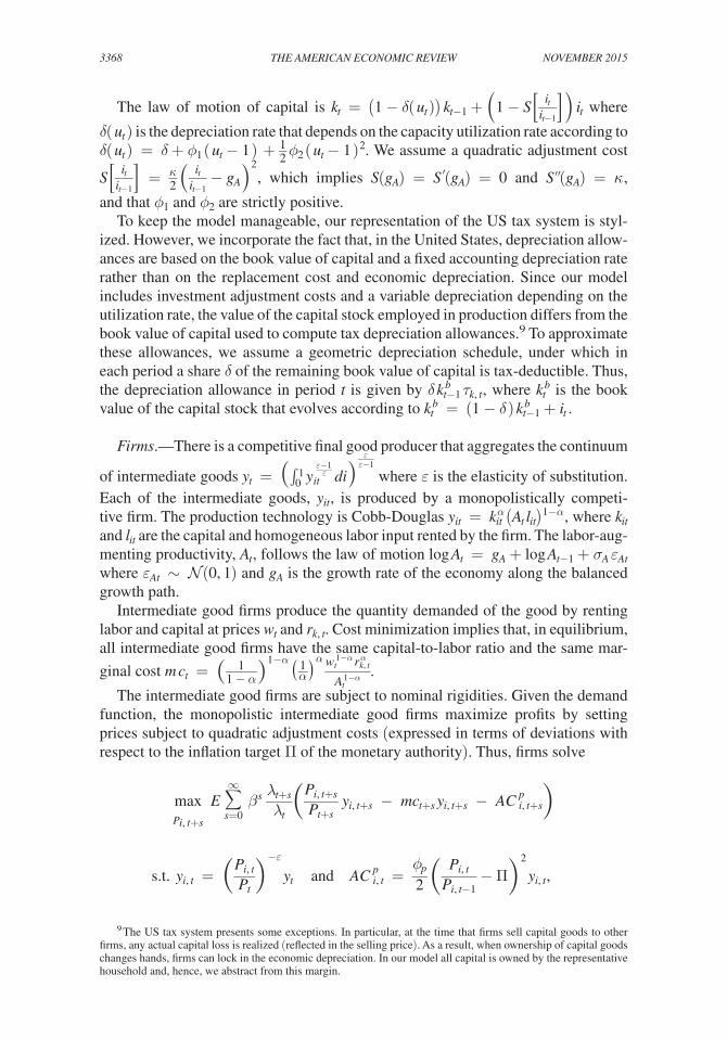
The law of motion of capital is k t = (1 − δ( u t )) k t−1 + (1 − S [ i t ___ i t−1
] ) i t where
δ( u t ) is the depreciation rate that depends on the capacity utilization rate according to δ( u t ) = δ + ϕ 1 ( u t − 1 ) + 1 _ 2 ϕ 2 ( u t − 1 ) 2 . We assume a quadratic adjustment cost
S [ i t ___ i t−1
] = κ _ 2 ( i t ___ i t−1 − g A )
2 , which implies S( g A ) = S ′ ( g A ) = 0 and S′′( g A ) = κ ,
and that ϕ 1 and ϕ 2 are strictly positive.To keep the model manageable, our representation of the US tax system is styl-
ized. However, we incorporate the fact that, in the United States, depreciation allow-ances are based on the book value of capital and a fixed accounting depreciation rate rather than on the replacement cost and economic depreciation. Since our model includes investment adjustment costs and a variable depreciation depending on the utilization rate, the value of the capital stock employed in production differs from the book value of capital used to compute tax depreciation allowances.9 To approximate these allowances, we assume a geometric depreciation schedule, under which in each period a share δ of the remaining book value of capital is tax-deductible. Thus, the depreciation allowance in period t is given by δ k t−1 b τ k, t , where k t b is the book value of the capital stock that evolves according to k t b = (1 − δ ) k t−1 b + i t .
Firms.—There is a competitive final good producer that aggregates the continuum
of intermediate goods y t = ( ∫ 0 1 y it ε−1 ___ ε di)
ε ___ ε−1 where ε is the elasticity of substitution.
Each of the intermediate goods, y it , is produced by a monopolistically competi-tive firm. The production technology is Cobb-Douglas y it = k it α ( A t l it ) 1−α , where k it and l it are the capital and homogeneous labor input rented by the firm. The labor-aug-menting productivity, A t , follows the law of motion log A t = g A + log A t−1 + σ A ε At where ε At ∼ (0, 1) and g A is the growth rate of the economy along the balanced growth path.
Intermediate good firms produce the quantity demanded of the good by renting labor and capital at prices w t and r k, t . Cost minimization implies that, in equilibrium, all intermediate good firms have the same capital-to-labor ratio and the same mar-
ginal cost m c t = ( 1 ___ 1 − α ) 1−α
( 1 __ α ) α w t 1−α r k, t α ______
A t 1−α .
The intermediate good firms are subject to nominal rigidities. Given the demand function, the monopolistic intermediate good firms maximize profits by setting prices subject to quadratic adjustment costs (expressed in terms of deviations with respect to the inflation target Π of the monetary authority). Thus, firms solve
max
P i, t+s E ∑
s=0
∞ β s λ t+s ___ λ t
( P i, t+s _____ P t+s
y i, t+s − m c t+s y i, t+s − A C i, t+s p )
s.t. y i, t = ( P i, t ___ P t
) −ε
y t and A C i, t p =
ϕ p ___ 2 (
P i, t _____ P i, t−1 − Π)
2
y i, t ,
9 The US tax system presents some exceptions. In particular, at the time that firms sell capital goods to other firms, any actual capital loss is realized (reflected in the selling price). As a result, when ownership of capital goods changes hands, firms can lock in the economic depreciation. In our model all capital is owned by the representative household and, hence, we abstract from this margin.
3369fernÁndez-villaverde et al.: shocks and activityvol. 105 no. 11
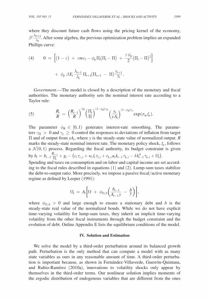
where they discount future cash flows using the pricing kernel of the economy,
β s λ t+s ___ λ t . After some algebra, the previous optimization problem implies an expanded
Phillips curve:
(4) 0 = [ (1 − ε) + εm c t − ϕ p Π t ( Π t − Π) + ε ϕ p ___ 2 ( Π t − Π) 2 ]
+ ϕ p β E t λ t+1 ____ λ t
Π t+1 ( Π t+1 − Π) y t+1 ____ y t .
Government.—The model is closed by a description of the monetary and fiscal authorities. The monetary authority sets the nominal interest rate according to a Taylor rule:
(5) R t __ R = ( R t−1 ____
R ) ϕ R
( Π t ___ Π ) (1− ϕ R ) γ Π
( y t ____ y A t
) (1− ϕ R ) γ y
exp ( σ m ξ t ).
The parameter ϕ R ∈ [0, 1) generates interest-rate smoothing. The parame-ters γ Π > 0 and γ y ≥ 0 control the responses to deviations of inflation from target Π and of output from y A t , where y is the steady-state value of normalized output. R marks the steady-state nominal interest rate. The monetary policy shock, ξ t , follows a (0, 1) process. Regarding the fiscal authority, its budget constraint is given
by b t = b t−1 R t−1 ___ Π t
+ g t − ( c t τ c, t + w t l t τ l, t + r k, t u t k t−1 τ k, t − δ k t−1 b τ k, t + Ω t ) .Spending and taxes on consumption and on labor and capital income are set accord-ing to the fiscal rules described in equations (1) and (2). Lump-sum taxes stabilize the debt-to-output ratio. More precisely, we impose a passive fiscal/active monetary regime as defined by Leeper (1991):
Ω t = A t [Ω + ϕ Ω, b ( b t−1 _____ A t−1 y − b __ y ) ] ,
where ϕ Ω, b > 0 and large enough to ensure a stationary debt and b is the steady-state real value of the normalized bonds. While we do not have explicit time-varying volatility for lump-sum taxes, they inherit an implicit time-varying volatility from the other fiscal instruments through the budget constraint and the evolution of debt. Online Appendix E lists the equilibrium conditions of the model.
IV. Solution and Estimation
We solve the model by a third-order perturbation around its balanced growth path. Perturbation is the only method that can compute a model with as many state variables as ours in any reasonable amount of time. A third-order perturba-tion is important because, as shown in Fernández-Villaverde, Guerrón-Quintana, and Rubio-Ramírez (2010a), innovations to volatility shocks only appear by themselves in the third-order terms. Our nonlinear solution implies moments of the ergodic distribution of endogenous variables that are different from the ones
3370 THE AMERICAN ECONOMIC REVIEW NOVEMbER 2015
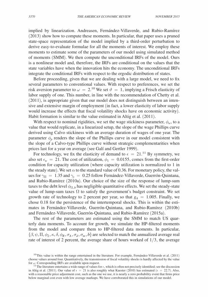
implied by linearization. Andreasen, Fernández-Villaverde, and Rubio-Ramírez (2013) show how to compute these moments. In particular, that paper uses a pruned state-space representation of the model implied by a third-order perturbation to derive easy-to-evaluate formulae for all the moments of interest. We employ these moments to estimate some of the parameters of our model using simulated method of moments (SMM). We then compute the unconditional IRFs of the model. Ours is a nonlinear model and, therefore, the IRFs are conditional on the values that the state variables have when the innovation hits the economy. The unconditional IRFs integrate the conditional IRFs with respect to the ergodic distribution of states.
Before proceeding, given that we are dealing with a large model, we need to fix several parameters to conventional values. With respect to preferences, we set the risk aversion parameter to ω = 2 .10 We set ϑ = 1 , implying a Frisch elasticity of labor supply of one. This number, in line with the recommendation of Chetty et al. (2011), is appropriate given that our model does not distinguish between an inten-sive and extensive margin of employment (in fact, a lower elasticity of labor supply would increase the effects that fiscal volatility shocks have on economic activity). Habit formation is similar to the value estimated in Altig et al. (2011).
With respect to nominal rigidities, we set the wage stickiness parameter, ϕ w , to a value that would replicate, in a linearized setup, the slope of the wage Phillips curve derived using Calvo stickiness with an average duration of wages of one year. The parameter ϕ p renders the slope of the Phillips curve in our model consistent with the slope of a Calvo-type Phillips curve without strategic complementarities when prices last for a year on average (see Galí and Gertler 1999).
For technology, we fix the elasticity of demand to ϵ = 21 .11 By symmetry, we also set ϵ w = 21 . The cost of utilization, ϕ 1 = 0.0155 , comes from the first-order condition for capacity utilization (where capacity utilization is normalized to 1 in the steady state). We set α to the standard value of 0.36 . For monetary policy, the val-ues for γ Π = 1.35 and γ y = 0.25 follow Fernández-Villaverde, Guerrón-Quintana, and Rubio-Ramírez (2010a). Our choice of the size of the response of lump-sum taxes to the debt level ϕ Ω, b has negligible quantitative effects. We set the steady-state value of lump-sum taxes Ω to satisfy the government’s budget constraint. We set growth rate of technology to 2 percent per year, so that g A = 1.005 . Finally, we chose 0.18 for the persistence of the intertemporal shocks. This is within the esti-mates in Fernández-Villaverde, Guerrón-Quintana, and Rubio-Ramírez (2010b) and Fernández-Villaverde, Guerrón-Quintana, and Rubio-Ramírez (2015a).
The rest of the parameters are estimated using the SMM to match US quar-terly data moments. To account for growth, we simulate the HP-filtered moments from the model and compare them to HP-filtered data moments. In particular, { β, ψ, Π, ϕ 2 , κ, δ, ϕ R , σ A , σ d , σ m , b} are selected to match the annualized average real rate of interest of 2 percent, the average share of hours worked of 1/3 , the average
10 This value is within the range entertained in the literature. For example, Fernández-Villaverde et al. (2011) choose values around four. Quantitatively, the transmission of fiscal volatility shocks is hardly affected by the value for ω . Corresponding IRFs are available upon request.
11 The literature entertains a wide range of values for ϵ , which is often not precisely identified; see the discussion in Altig et al. (2011). Our value of ϵ = 21 is also roughly what Kuester (2010) has estimated ( ϵ = 22.7 ). Also, with a reasonable price adjustment cost, such as the one we use, it is nearly a zero probability event that firms price below marginal cost even with low average markups. We have corroborated this in simulations of our model.
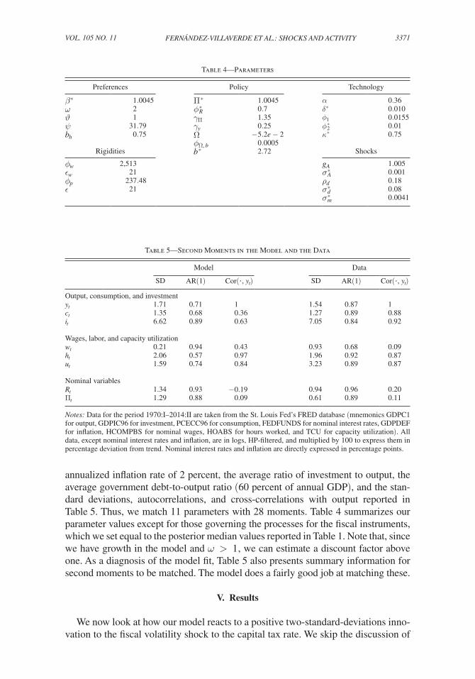
3371fernÁndez-villaverde et al.: shocks and activityvol. 105 no. 11
annualized inflation rate of 2 percent, the average ratio of investment to output, the average government debt-to-output ratio (60 percent of annual GDP), and the stan-dard deviations, autocorrelations, and cross-correlations with output reported in Table 5. Thus, we match 11 parameters with 28 moments. Table 4 summarizes our parameter values except for those governing the processes for the fiscal instruments, which we set equal to the posterior median values reported in Table 1. Note that, since we have growth in the model and ω > 1 , we can estimate a discount factor above one. As a diagnosis of the model fit, Table 5 also presents summary information for second moments to be matched. The model does a fairly good job at matching these.
V. Results
We now look at how our model reacts to a positive two-standard-deviations inno-vation to the fiscal volatility shock to the capital tax rate. We skip the discussion of
Table 4—Parameters
Preferences Policy Technology
β ∗ 1.0045 Π ∗ 1.0045 α 0.36 ω 2 ϕ R ∗ 0.7 δ ∗ 0.010 ϑ 1 γ Π 1.35 ϕ 1 0.0155 ψ 31.79 γ y 0.25 ϕ 2 ∗ 0.01 b h 0.75 Ω − 5.2e − 2 κ ∗ 0.75
ϕ Ω, b 0.0005 Rigidities b ∗ 2.72 Shocks
ϕ w 2,513 g A 1.005 ϵ w 21 σ A ∗ 0.001 ϕ p 237.48 ρ d 0.18 ϵ 21 σ d ∗ 0.08
σ m ∗ 0.0041
Table 5—Second Moments in the Model and the Data
Model Data
SD AR(1) Cor( · , y t ) SD AR(1) Cor( · , y t )
Output, consumption, and investment y t 1.71 0.71 1 1.54 0.87 1 c t 1.35 0.68 0.36 1.27 0.89 0.88 i t 6.62 0.89 0.63 7.05 0.84 0.92
Wages, labor, and capacity utilization w t 0.21 0.94 0.43 0.93 0.68 0.09 h t 2.06 0.57 0.97 1.96 0.92 0.87 u t 1.59 0.74 0.84 3.23 0.89 0.87
Nominal variables R t 1.34 0.93 −0.19 0.94 0.96 0.20 Π t 1.29 0.88 0.09 0.61 0.89 0.11
Notes: Data for the period 1970:I–2014:II are taken from the St. Louis Fed’s FRED database (mnemonics GDPC1 for output, GDPIC96 for investment, PCECC96 for consumption, FEDFUNDS for nominal interest rates, GDPDEF for inflation, HCOMPBS for nominal wages, HOABS for hours worked, and TCU for capacity utilization). All data, except nominal interest rates and inflation, are in logs, HP-filtered, and multiplied by 100 to express them in percentage deviation from trend. Nominal interest rates and inflation are directly expressed in percentage points.
3372 THE AMERICAN ECONOMIC REVIEW NOVEMbER 2015
other instruments because, in preliminary work, we ascertained that their effects were smaller.
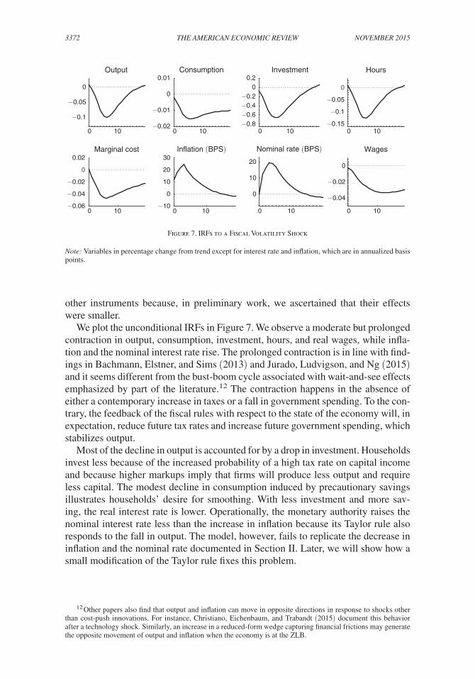
We plot the unconditional IRFs in Figure 7. We observe a moderate but prolonged contraction in output, consumption, investment, hours, and real wages, while infla-tion and the nominal interest rate rise. The prolonged contraction is in line with find-ings in Bachmann, Elstner, and Sims (2013) and Jurado, Ludvigson, and Ng (2015) and it seems different from the bust-boom cycle associated with wait-and-see effects emphasized by part of the literature.12 The contraction happens in the absence of either a contemporary increase in taxes or a fall in government spending. To the con-trary, the feedback of the fiscal rules with respect to the state of the economy will, in expectation, reduce future tax rates and increase future government spending, which stabilizes output.
Most of the decline in output is accounted for by a drop in investment. Households invest less because of the increased probability of a high tax rate on capital income and because higher markups imply that firms will produce less output and require less capital. The modest decline in consumption induced by precautionary savings illustrates households’ desire for smoothing. With less investment and more sav-ing, the real interest rate is lower. Operationally, the monetary authority raises the nominal interest rate less than the increase in inflation because its Taylor rule also responds to the fall in output. The model, however, fails to replicate the decrease in inflation and the nominal rate documented in Section II. Later, we will show how a small modification of the Taylor rule fixes this problem.
12 Other papers also find that output and inflation can move in opposite directions in response to shocks other than cost-push innovations. For instance, Christiano, Eichenbaum, and Trabandt (2015) document this behavior after a technology shock. Similarly, an increase in a reduced-form wedge capturing financial frictions may generate the opposite movement of output and inflation when the economy is at the ZLB.
Hours
0 10
−0.1
−0.05
0
0 10−0.02
−0.01
0
0.01
0 10−0.8−0.6−0.4−0.2
00.2
0 10−0.15
−0.1
−0.05
0
0 10−0.06
−0.04
−0.02
0
0.02
0 10−10
0
10
20
30
0 10
0
10
20
0 10
−0.04
−0.02
0
Output Consumption Investment
WagesMarginal cost In�ation (BPS) Nominal rate (BPS)
Figure 7. IRFs to a Fiscal Volatility Shock
Note: Variables in percentage change from trend except for interest rate and inflation, which are in annualized basis points.
3373fernÁndez-villaverde et al.: shocks and activityvol. 105 no. 11
In online Appendix F, we document that the effects reported in Figure 7 are roughly equivalent to the effects of an unexpected 30-basis-point (annualized) increase in the nominal interest rate implied by our VAR in Section II and by Altig et al.’s (2011) VAR. We picked a 30-basis-point increase in the federal funds rate because it corresponds to a monetary policy shock as typically identified in empirical studies.
A central transmission mechanism, which we will discuss below in detail, is a rise in markups. This is illustrated by the first panel of the bottom row in Figure 7, which shows that real marginal costs fall. With Rotemberg pricing, the gross markup equals the inverse of real marginal costs. Thus, the model matches the results of rais-ing markups documented in Section II. Markups work like a distortionary wedge that reduces labor supply. A higher wedge generates a positive co-movement between consumption and output that was difficult to deliver in Bloom (2009).
An Alternative Taylor Rule.—The baseline economy fails to replicate one of the features of the VAR presented in Section II, namely, the decrease in inflation and the nominal rate. Yet, a small modification of the Taylor rule reconciles the model with the VAR evidence. In particular, let us now consider that the monetary authority reacts to fiscal volatility shocks and, instead of following equation (5), it sets the nominal interest rate according to
(6) R t __ R = ( R t−1 ____
R ) ϕ R
( Π t ___ Π ) (1− ϕ R ) γ Π
( y t ____ y A t
) (1− ϕ R ) γ y
( e σ τ k, t ____ e σ τ k )
γ σ (1− ϕ R ) exp ( σ m ξ t ) .
We are motivated in our choice of equation (6) by the observation that the minutes of the FOMC have, on many occasions both before and after the recent financial crisis, explicitly mentioned fiscal policy uncertainty and its impact on consumption and investment as a consideration for monetary policymaking. For example, on January 30–31, 1996, the concerns that the FOMC members expressed about fiscal policy volatility (“The outlook for fiscal policy was uncertain”) may account for an easing of monetary policy that was smaller than the one expected by the futures market or the one that a simple Taylor rule would have dictated (see Dueker and Fischer 1997 for details.)13 We call the model with the new Taylor rule the extended economy.
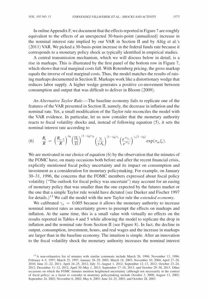
We calibrated γ σ = 0.005 because it allows the monetary authority to increase nominal interest rates as uncertainty grows to preempt the effects on markups and inflation. At the same time, this is a small value with virtually no effects on the results reported in Tables 4 and 5 while allowing the model to replicate the drop in inflation and the nominal rate from Section II (see Figure 8). In fact, the decline in output, consumption, investment, hours, and real wages and the increase in markups are larger than in the baseline economy. The intuition is simple. After an innovation to the fiscal volatility shock the monetary authority increases the nominal interest
13 A non-exhaustive list of minutes with similar comments include March 26, 1996; November 13, 1996; February 4–5, 1997; March 25, 1997; January 28–29, 2003; March 18, 2003; November 10, 2004; April 27–28, 2010; June 21–22, 2011; April 24–25, 2012; July 31–August 1, 2012; September 12–13, 2012; October 23–24, 2012; December 11–12, 2012; April 30–May 1, 2013; September 17–18, 2013; and October 29–30, 2013. Other occasions on which the FOMC minutes mention heightened uncertainty (although not necessarily in the context of fiscal policy) as a factor to consider in monetary policymaking include October 3, 2000; August 13, 2002; September 24, 2002; November 6, 2002; May 6, 2003; June 24–25, 2003; and October 28, 2003.
3374 THE AMERICAN ECONOMIC REVIEW NOVEMbER 2015
rate more than it would otherwise do. This increase further depresses aggregate demand and the marginal cost. The lower marginal cost is translated into a fall in inflation. The higher nominal interest rate and lower inflation mean a higher real interest rate and, with it, the larger contraction in output.
VI. Accounting for the Rise in Markups
Why do markups increase after a fiscal volatility shock? Because of two chan-nels: an aggregate demand channel and an upward pricing bias channel. Both of these are related to nominal rigidities. We start with the fall in aggregate demand. As we argued before, faced with higher uncertainty, households want to consume and invest less. In the absence of nominal rigidities, the effect of the scramble to lower consumption and investment would be small. With rigidities, however, prices do not fully accommodate the lower demand. Thus, markups rise and output falls.
The upward pricing bias channel leads firms, after a fiscal volatility shock, to set prices higher than they would otherwise do. With Rotemberg adjustment costs, the price that the firm sets today determines how costly it will be to change to a new price tomorrow. But because the profit function is asymmetric (it is more costly for the firm to set too low a price relative to its competitors, rather than setting it too high), firms bias their pricing decision today upward.
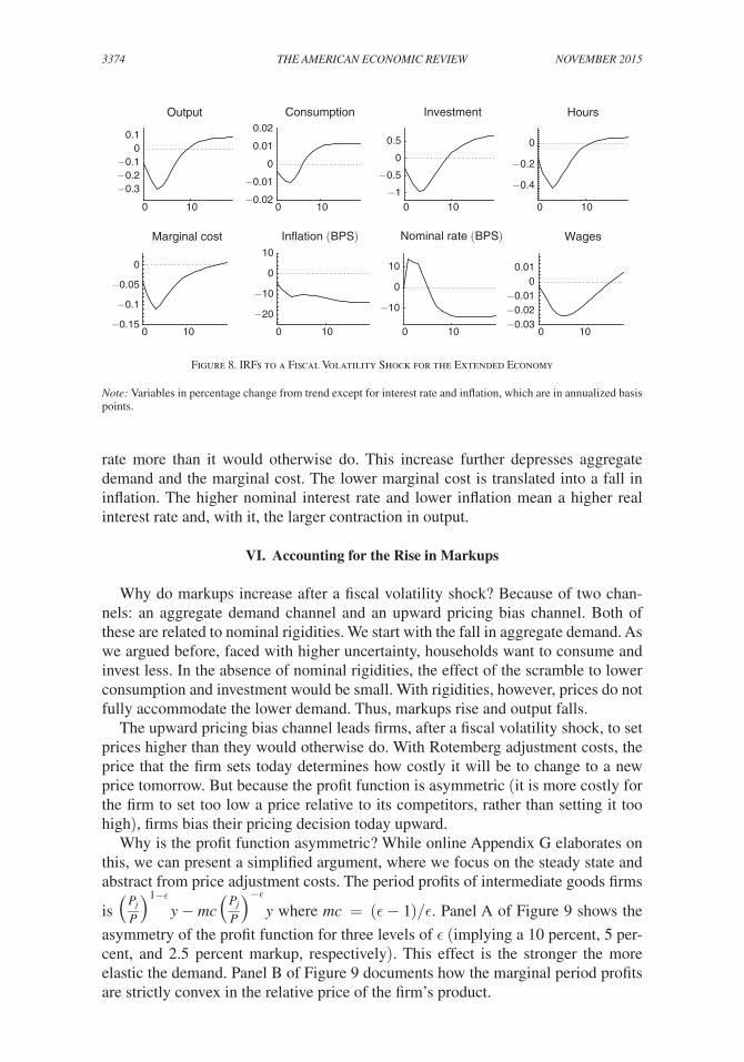
Why is the profit function asymmetric? While online Appendix G elaborates on this, we can present a simplified argument, where we focus on the steady state and abstract from price adjustment costs. The period profits of intermediate goods firms
is ( P j __ P )
1−ϵ y − mc (
P j __ P ) −ϵ
y where mc = (ϵ − 1)/ϵ . Panel A of Figure 9 shows the
asymmetry of the profit function for three levels of ϵ (implying a 10 percent, 5 per-cent, and 2.5 percent markup, respectively). This effect is the stronger the more elastic the demand. Panel B of Figure 9 documents how the marginal period profits are strictly convex in the relative price of the firm’s product.
0 10
−0.3−0.2−0.1
00.1
0 10−0.02
−0.01
0
0.01
0.02
0 10−1
−0.5
0
0.5
0 10
−0.4
−0.2
0
0 10−0.15
−0.1
−0.05
0
0 10
−20
−10
0
10
0 10
−10
0
10
0 10−0.03−0.02−0.01
00.01
HoursOutput Consumption Investment
WagesMarginal cost In�ation (BPS) Nominal rate (BPS)
Figure 8. IRFs to a Fiscal Volatility Shock for the Extended Economy
Note: Variables in percentage change from trend except for interest rate and inflation, which are in annualized basis points.
3375fernÁndez-villaverde et al.: shocks and activityvol. 105 no. 11
A fiscal volatility shock increases the dispersion of future capital income tax rates and with them, the dispersion of future marginal costs and the probable range for the optimal price tomorrow. Firms respond by biasing their pricing decision upward more than they would do otherwise. Realized marginal costs fall because firms, given the fall in output, rent less capital and this lowers the rental rates. Wages, subject to rigidities, barely move and the labor market clears through a reduction in hours worked. Higher prices and lower marginal costs produce a rise in markups.
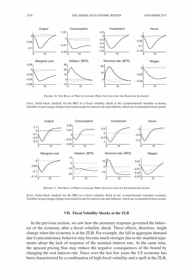
Figure 10 gauges how important the upward pricing bias channel is by compar-ing the IRFs to a fiscal volatility shock in the baseline economy (solid line) and in a counterfactual one (dashed line). All the equilibrium conditions of the counter-factual economy are the same as in the baseline economy except that now inflation evolves according to the linearized version of the Phillips curve (4) that eliminates the nonlinear terms that induce the upward pricing bias:
(7) Π t − Π = β E t ( Π t+1 − Π) + ϵ ____ ϕ p Π (m c t − mc) .
However, since we solve the rest of the model through a third-order expansion, the demand channel of fiscal volatility shocks is still present. Figure 10 underlines the importance of the upward pricing bias on the baseline economy. When the bias is not present, output rises marginally due to an increase in hours. Precautionary behavior leads households to supply more hours when fiscal volatility is high. In comparison, when the upward pricing bias is present, the wedge caused by higher markups overcomes this precautionary behavior and hours worked fall on impact.
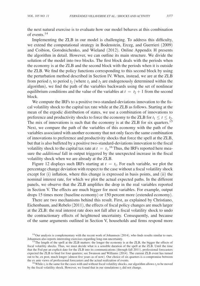
In comparison, the aggregate demand channel is more important in the extended economy (see Figure 11). The fact that the monetary authority reacts directly to fiscal volatility shocks ameliorates the upward pricing bias channel. And, at the same time, the increase in the real interest rate considerably strengthens the fall in aggregate demand.
0.95 1 1.05−0.2
−0.15
−0.1
−0.05
0
0.05
11
21
41
0.95 1 1.050
5
10
15
41
21
11
Relative price (Pj/P) Relative price (Pj/P)
Panel A. Period pro�ts Panel B. Marginal period pro�ts
Figure 9. Properties of the Profit Function
Note: Profit function and marginal period profits for different demand elasticities as functions of the relative price.
3376 THE AMERICAN ECONOMIC REVIEW NOVEMbER 2015
VII. Fiscal Volatility Shocks at the ZLB
In the previous section, we saw how the monetary response governed the behav-ior of the economy after a fiscal volatility shock. These effects, therefore, might change when the economy is at the ZLB. For example, the fall in aggregate demand due to precautionary behavior may become much stronger due to the standard argu-ments about the lack of response of the nominal interest rate. At the same time, the upward pricing bias may reduce the negative consequences of the bound by changing the real interest rate. Since over the last few years the US economy has been characterized by a combination of high fiscal volatility and a spell at the ZLB,
0 10
−0.1
−0.05
0
0 10−0.02
−0.01
0
0.01
0 10−0.8−0.6−0.4−0.2
00.2
0 10−0.15
−0.1
−0.05
0
0 10−0.06
−0.04
−0.02
0
0.02
0 10−10
0
10
20
30
0 10
0
10
20
0 10
−0.04
−0.02
0
HoursOutput Consumption Investment
WagesMarginal cost In�ation (BPS) Nominal rate (BPS)
Figure 10. The Role of Precautionary Price Setting for the Baseline Economy
Notes: Solid black (dashed) for the IRFs to a fiscal volatility shock in the (counterfactual) baseline economy. Variables in percentage change from trend except for interest rate and inflation, which are in annualized basis points.
0 10
−0.3−0.2−0.1
00.1
0 10−0.02
−0.01
0
0.01
0.02
0 10−1
−0.5
0
0.5
0 10
−0.4
−0.2
0
0 10−0.15
−0.1
−0.05
0
0 10
−20
−10
0
10
0 10
−10
0
10
0 10−0.03−0.02−0.01
00.01
HoursOutput Consumption Investment
WagesMarginal cost In�ation (BPS) Nominal rate (BPS)
Figure 11. The Role of Precautionary Price Setting for the Extended Economy
Notes: Solid black (dashed) for the IRFs to a fiscal volatility shock in the (counterfactual) extended economy. Variables in percentage change from trend except for interest rate and inflation, which are in annualized basis points.
3377fernÁndez-villaverde et al.: shocks and activityvol. 105 no. 11
the next natural exercise is to evaluate how our model behaves at this combination of events.14
Implementing the ZLB in our model is challenging. To address this difficulty, we extend the computational strategy in Bodenstein, Erceg, and Guerrieri (2009) and Coibion, Gorodnichenko, and Wieland (2012). Online Appendix H presents the algorithm in detail. However, we can outline its main structure. We divide the solution of the model into two blocks. The first block deals with the periods when the economy is at the ZLB and the second block with the periods when it is outside the ZLB. We find the policy functions corresponding to this second block by using the perturbation method described in Section IV. When, instead, we are at the ZLB from period t 1 to period t 2 (where t 1 and t 2 are endogenously determined within the algorithm), we find the path of the variables backwards using the set of nonlinear equilibrium conditions and the value of the variables at t = t 2 + 1 from the second block.
We compute the IRFs to a positive two-standard-deviations innovation to the fis-cal volatility shock to the capital tax rate while at the ZLB as follows. Starting at the mean of the ergodic distribution of states, we use a combination of innovations to preference and productivity shocks to force the economy to the ZLB for t 1 ≤ t ≤ t 2 . The mix of innovations is such that the economy is at the ZLB for six quarters.15 Next, we compare the path of the variables of this economy with the path of the variables associated with another economy that not only faces the same combination of innovations to preference and productivity shocks that force the spell at the ZLB, but that is also buffeted by a positive two-standard-deviations innovation to the fiscal volatility shock to the capital tax rate at t = t 1 .16 Thus, the IRFs reported here mea-sure the additional fall in output triggered by the unexpected increase in the fiscal volatility shock when we are already at the ZLB.
Figure 12 displays such IRFs starting at t = t 1 . For each variable, we plot the percentage change deviation with respect to the case without a fiscal volatility shock except for (i) inflation, where this change is expressed in basis points, and (ii) the nominal interest rate, for which we plot the actual expected paths. In the different panels, we observe that the ZLB amplifies the drop in the real variables reported in Section V. The effects are much bigger for most variables. For example, output drops 15 times more (baseline economy) or 150 percent more (extended economy).
There are two mechanisms behind this result. First, as explained by Christiano, Eichenbaum, and Rebelo (2011), the effects of fiscal policy changes are much larger at the ZLB: the real interest rate does not fall after a fiscal volatility shock to undo the contractionary effects of heightened uncertainty. Consequently, and because of the same arguments outlined in Section V, households and firms respond more
14 Our analysis is complementary with the recent work of Johannsen (2014), who finds results similar to ours. Johannsen also reports interesting exercises regarding long-run uncertainty.
15 The length of the spell at the ZLB matters: the longer the economy is at the ZLB, the bigger the effects of fiscal volatility shocks. Thus, we must decide what is a sensible duration of the spell at the ZLB. Until the time that the Fed put an explicit date for the ZLB into its communications (through fall 2011), professional forecasters expected the ZLB to bind for four quarters; see Swanson and Williams (2014). The current ZLB event has turned out to be, ex post, much longer (almost five years as of now). Our choice of six quarters is a compromise between the ex ante views of professional forecasters and the actual realization of events.
16 While t 1 is the same for the cases with and without fiscal volatility shocks, our algorithm allows t 2 to be moved by the fiscal volatility shock. However, we found that in our simulations t 2 did not change.
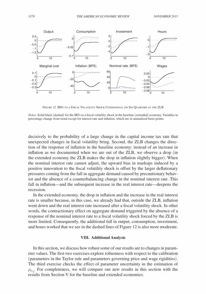
3378 THE AMERICAN ECONOMIC REVIEW NOVEMbER 2015
decisively to the probability of a large change in the capital income tax rate that unexpected changes in fiscal volatility bring. Second, the ZLB changes the direc-tion of the response of inflation in the baseline economy: instead of an increase in inflation as we documented when we are out of the ZLB, we observe a drop (in the extended economy the ZLB makes the drop in inflation slightly bigger). When the nominal interest rate cannot adjust, the upward bias in markups induced by a positive innovation to the fiscal volatility shock is offset by the larger deflationary pressures coming from the fall in aggregate demand caused by precautionary behav-ior and the absence of a counterbalancing change in the nominal interest rate. This fall in inflation—and the subsequent increase in the real interest rate—deepens the recession.
In the extended economy, the drop in inflation and the increase in the real interest rate is smaller because, in this case, we already had that, outside the ZLB, inflation went down and the real interest rate increased after a fiscal volatility shock. In other words, the contractionary effect on aggregate demand triggered by the absence of a response of the nominal interest rate to a fiscal volatility shock forced by the ZLB is more limited. Consequently, the additional fall in output, consumption, investment, and hours worked that we see in the dashed lines of Figure 12 is also more moderate.
VIII. Additional Analysis
In this section, we discuss how robust some of our results are to changes in param-eter values. The first two exercises explore robustness with respect to the calibration (parameters in the Taylor rule and parameters governing price and wage rigidities). The third exercise checks the effect of parameter uncertainty in the estimation of ρ σ τ k . For completeness, we will compare our new results in this section with the results from Section V for the baseline and extended economies.
0 10
−1.5−1
−0.50
0.5
0 10−0.1
−0.05
0
0 10
−4
−2
0
2
0 10−2
−1
0
0 10
−0.3−0.2−0.1
00.1
0 10
−40
−20
0
0 10
0
20
40
60
0 10−0.08−0.06−0.04−0.02
00.02
HoursOutput Consumption Investment
WagesMarginal cost In�ation (BPS) Nominal rate (BPS)
Figure 12. IRFs to a Fiscal Volatility Shock Conditional on Six Quarters at the ZLB
Notes: Solid black (dashed) for the IRFs to a fiscal volatility shock in the baseline (extended) economy. Variables in percentage change from trend except for interest rate and inflation, which are in annualized basis points.
3379fernÁndez-villaverde et al.: shocks and activityvol. 105 no. 11
A. The Role of Monetary Policy
How should policymakers respond to unexpected changes in fiscal volatility shocks? While a full optimal policy design exercise is beyond the scope of this paper, we can at least evaluate the response of the economy under different values of the parameters on the Taylor rule. In that way, we can start understanding some of the choices faced by the monetary authority.
The IRFs in Figures 13 and 14 show two alternative scenarios for the baseline and extended economies, respectively. In the first scenario, the monetary authority reacts more strongly to output (a value of γ y = 0.5 instead of γ y = 0.25 , dashed lines). In the second scenario, the monetary authority reacts more aggressively to inflation (a value of γ Π = 1.5 instead of γ Π = 1.25, dotted lines). When the response to output in the Taylor rule ( γ y ) is high in the baseline economy, firms anticipate that inflation will be tolerated. To counterbalance declining profits, firms aggressively increase prices with a view toward higher markups. Firms’ anticipation of a loose stance of monetary policy results in higher inflation and lower output. An accom-modative monetary policy, then, exacerbates the effects. In contrast, if the central bank assigns less weight to stabilizing output, firms consider future inflation less likely, which reduces the upward pricing bias. The smaller the monetary response to output, the more moderate is the inflation response and the contraction in output. An analogous argument explains why a stronger focus of monetary policy on infla-tion alleviates the negative outcomes on output and stabilizes inflation. Therefore, unexpected changes in fiscal volatility shocks do not create a trade-off between stabilizing output and inflation, as we would have, for instance, with markup shocks.
In the extended economy, since the monetary authority is already reacting to fis-cal policy volatility, the differences among the three cases are smaller for the real variables. A fiscal volatility shock translates, ceteris paribus, into a higher nom-inal interest rate at impact regardless of the values of γ y and γ Π . The increase in nominal interest rates lowers the upward pricing bias of firms and with it, inflation and the contractionary effects of fiscal volatility shocks. The variations in the level of γ y and γ Π lead to variations in how fast the nominal rate falls after its increase at impact. When γ y is high, the nominal interest rate falls faster and, when γ Π is high, it falls more slowly. Given the small change in consumption levels, and through a Fisher-equation type of argument, how fast inflation falls is closely linked with the speed of the fall in the nominal interest rate.
B. The Role of Price and Wage Rigidities
Section V highlighted the importance of rigidities in accounting for the effects of unexpected changes in fiscal volatility shocks. Figures 15 and 16 illustrate this point for the baseline and extended economy, respectively. The dashed line plots the IRFs when we reduce price stickiness to the one equivalent to a Calvo model with an average price duration of about one quarter. The response is less pronounced and shorter-lived. The dotted line in turn plots the IRFs when we reduce wage stickiness to an equivalent Calvo model with an average wage duration of about one quarter. As with more flexible prices, the response is less pronounced. Finally, the squared line reduces both price and wage stickiness to the low values mentioned above. In
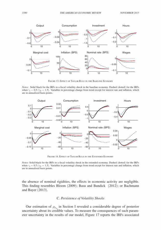
3380 THE AMERICAN ECONOMIC REVIEW NOVEMbER 2015
the absence of nominal rigidities, the effects in economic activity are negligible. This finding resembles Bloom (2009); Basu and Bundick (2012); or Bachmann and Bayer (2013).
C. Persistence of Volatility Shocks
Our estimation of ρ σ τ k in Section I revealed a considerable degree of posterior uncertainty about its credible values. To measure the consequences of such param-eter uncertainty in the results of our model, Figure 17 reports the IRFs associated
0 10−0.2
−0.1
0
0 10
−0.04
−0.02
0
0 10
−1.5
−1
−0.5
0
0 10
−0.2
−0.1
0
0 10−0.1
−0.05
0
0 10
0
50
100
0 10
020406080
0 10−0.1
−0.05
0
HoursOutput Consumption Investment
WagesMarginal cost In�ation (BPS) Nominal rate (BPS)
0 10
−0.3−0.2−0.1
00.1
0 10−0.02
−0.01
0
0.01
0.02
0 10
−1
−0.5
0
0.5
0 10
−0.4
−0.2
0
0 10−0.15
−0.1
−0.05
0
0 10−60
−40
−20
0
0 10−60
−40
−20
0
0 10
−0.02
0
0.02
0.04
HoursOutput Consumption Investment
WagesMarginal cost In�ation (BPS) Nominal rate (BPS)
Figure 13. Effect of Taylor Rule in the Baseline Economy
Notes: Solid black for the IRFs to a fiscal volatility shock in the baseline economy. Dashed (dotted) for the IRFs when γ y = 0.5 ( γ Π = 1.5). Variables in percentage change from trend except for interest rate and inflation, which are in annualized basis points.
Figure 14. Effect of Taylor Rule in the Extended Economy
Notes: Solid black for the IRFs to a fiscal volatility shock in the extended economy. Dashed (dotted) for the IRFs when γ y = 0.5 ( γ Π = 1.5). Variables in percentage change from trend except for interest rate and inflation, which are in annualized basis points.
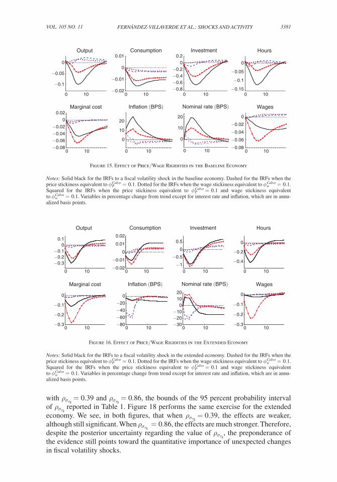
3381fernÁndez-villaverde et al.: shocks and activityvol. 105 no. 11
with ρ σ τ k = 0.39 and ρ σ τ k = 0.86, the bounds of the 95 percent probability interval of ρ σ τ k reported in Table 1. Figure 18 performs the same exercise for the extended economy. We see, in both figures, that when ρ σ τ k = 0.39, the effects are weaker, although still significant. When ρ σ τ k = 0.86, the effects are much stronger. Therefore, despite the posterior uncertainty regarding the value of ρ σ τ k , the preponderance of the evidence still points toward the quantitative importance of unexpected changes in fiscal volatility shocks.
0 10
−0.1
−0.05
0
0 10−0.02
−0.01
0
0.01
0 10−0.8−0.6−0.4−0.2
00.2
0 10−0.15
−0.1
−0.05
0
0 10−0.08
−0.06
−0.04
−0.02
0
0.02
0 10
0
10
20
0 10
0
10
20
0 10−0.08
−0.06
−0.04
−0.02
0
HoursOutput Consumption Investment
WagesMarginal cost In�ation (BPS) Nominal rate (BPS)
0 10
−0.3−0.2−0.1
00.1
0 10−0.02
−0.01
0
0.01
0.02
0 10−1
−0.5
0
0.5
0 10
−0.4
−0.2
0
0 10−0.3
−0.2
−0.1
0
0 10−80
−60
−40
−20
0
0 10−30−20−10
01020
0 10−0.3
−0.2
−0.1
0
HoursOutput Consumption Investment
WagesMarginal cost In�ation (BPS) Nominal rate (BPS)
Figure 15. Effect of Price/Wage Rigidities in the Baseline Economy
Notes: Solid black for the IRFs to a fiscal volatility shock in the baseline economy. Dashed for the IRFs when the price stickiness equivalent to ϕ P Calvo = 0.1. Dotted for the IRFs when the wage stickiness equivalent to ϕ w Calvo = 0.1. Squared for the IRFs when the price stickiness equivalent to ϕ P Calvo = 0.1 and wage stickiness equivalent to ϕ w Calvo = 0.1. Variables in percentage change from trend except for interest rate and inflation, which are in annu-alized basis points.
Figure 16. Effect of Price/Wage Rigidities in the Extended Economy
Notes: Solid black for the IRFs to a fiscal volatility shock in the extended economy. Dashed for the IRFs when the price stickiness equivalent to ϕ P Calvo = 0.1. Dotted for the IRFs when the wage stickiness equivalent to ϕ w Calvo = 0.1. Squared for the IRFs when the price stickiness equivalent to ϕ P Calvo = 0.1 and wage stickiness equivalent to ϕ w Calvo = 0.1. Variables in percentage change from trend except for interest rate and inflation, which are in annu-alized basis points.
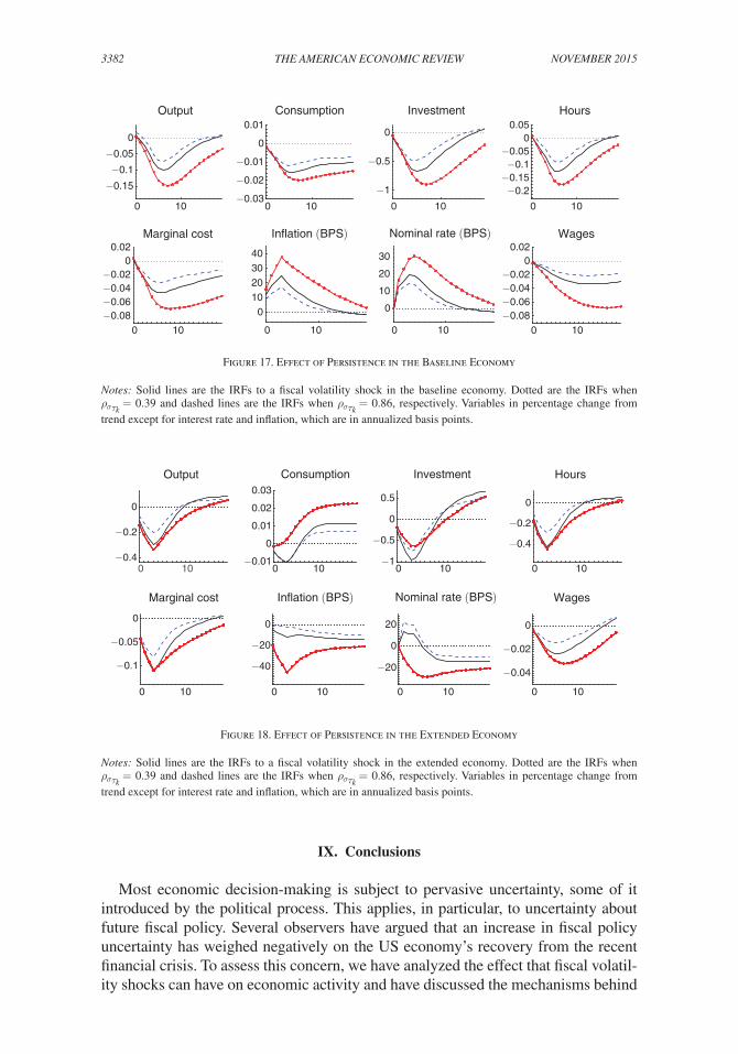
3382 THE AMERICAN ECONOMIC REVIEW NOVEMbER 2015
IX. Conclusions
Most economic decision-making is subject to pervasive uncertainty, some of it introduced by the political process. This applies, in particular, to uncertainty about future fiscal policy. Several observers have argued that an increase in fiscal policy uncertainty has weighed negatively on the US economy’s recovery from the recent financial crisis. To assess this concern, we have analyzed the effect that fiscal volatil-ity shocks can have on economic activity and have discussed the mechanisms behind
0 10
−0.15
−0.1
−0.05
0
0 10−0.03
−0.02
−0.01
0
0.01
0 10
−1
−0.5
0
0 10
−0.2−0.15−0.1
−0.050
0.05
0 10−0.08−0.06−0.04−0.02
00.02
0 10
010203040
0 10
0
10
20
30
0 10−0.08−0.06−0.04−0.02
00.02
HoursOutput Consumption Investment
WagesMarginal cost In�ation (BPS) Nominal rate (BPS)
0 10−0.4
−0.2
0
0 10−0.01
0
0.01
0.02
0.03
0 10−1
−0.5
0
0.5
0 10
−0.4
−0.2
0
0 10
−0.1
−0.05
0
0 10
−40
−20
0
0 10
−20
0
20
0 10
−0.04
−0.02
0
HoursOutput Consumption Investment
WagesMarginal cost In�ation (BPS) Nominal rate (BPS)
Figure 17. Effect of Persistence in the Baseline Economy
Notes: Solid lines are the IRFs to a fiscal volatility shock in the baseline economy. Dotted are the IRFs when ρ σ τ k = 0.39 and dashed lines are the IRFs when ρ σ τ k = 0.86 , respectively. Variables in percentage change from trend except for interest rate and inflation, which are in annualized basis points.
Figure 18. Effect of Persistence in the Extended Economy
Notes: Solid lines are the IRFs to a fiscal volatility shock in the extended economy. Dotted are the IRFs when ρ σ τ k = 0.39 and dashed lines are the IRFs when ρ σ τ k = 0.86 , respectively. Variables in percentage change from trend except for interest rate and inflation, which are in annualized basis points.
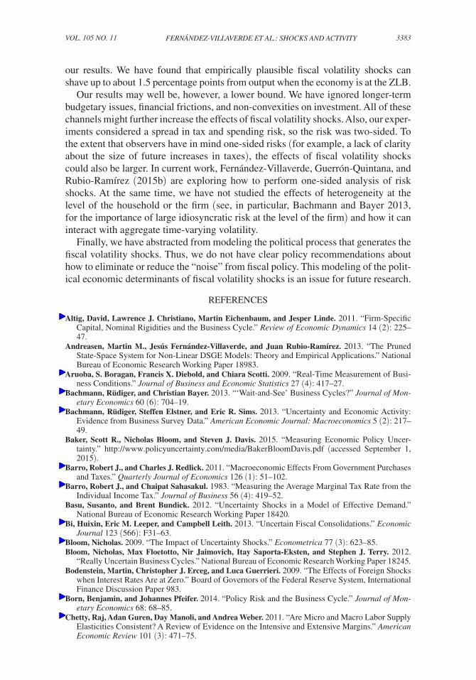
3383fernÁndez-villaverde et al.: shocks and activityvol. 105 no. 11
our results. We have found that empirically plausible fiscal volatility shocks can shave up to about 1.5 percentage points from output when the economy is at the ZLB.
Our results may well be, however, a lower bound. We have ignored longer-term budgetary issues, financial frictions, and non-convexities on investment. All of these channels might further increase the effects of fiscal volatility shocks. Also, our exper-iments considered a spread in tax and spending risk, so the risk was two-sided. To the extent that observers have in mind one-sided risks (for example, a lack of clarity about the size of future increases in taxes), the effects of fiscal volatility shocks could also be larger. In current work, Fernández-Villaverde, Guerrón-Quintana, and Rubio-Ramírez (2015b) are exploring how to perform one-sided analysis of risk shocks. At the same time, we have not studied the effects of heterogeneity at the level of the household or the firm (see, in particular, Bachmann and Bayer 2013, for the importance of large idiosyncratic risk at the level of the firm) and how it can interact with aggregate time-varying volatility.
Finally, we have abstracted from modeling the political process that generates the fiscal volatility shocks. Thus, we do not have clear policy recommendations about how to eliminate or reduce the “noise” from fiscal policy. This modeling of the polit-ical economic determinants of fiscal volatility shocks is an issue for future research.
REFERENCES
Altig, David, Lawrence J. Christiano, Martin Eichenbaum, and Jesper Linde. 2011. “Firm-Specific Capital, Nominal Rigidities and the Business Cycle.” Review of Economic Dynamics 14 (2): 225–47.
Andreasen, Martin M., Jesús Fernández-Villaverde, and Juan Rubio-Ramírez. 2013. “The Pruned State-Space System for Non-Linear DSGE Models: Theory and Empirical Applications.” National Bureau of Economic Research Working Paper 18983.
Aruoba, S. Boragan, Francis X. Diebold, and Chiara Scotti. 2009. “Real-Time Measurement of Busi-ness Conditions.” Journal of Business and Economic Statistics 27 (4): 417–27.
Bachmann, Rüdiger, and Christian Bayer. 2013. “‘Wait-and-See’ Business Cycles?” Journal of Mon-etary Economics 60 (6): 704–19.
Bachmann, Rüdiger, Steffen Elstner, and Eric R. Sims. 2013. “Uncertainty and Economic Activity: Evidence from Business Survey Data.” American Economic Journal: Macroeconomics 5 (2): 217–49.
Baker, Scott R., Nicholas Bloom, and Steven J. Davis. 2015. “Measuring Economic Policy Uncer-tainty.” http://www.policyuncertainty.com/media/BakerBloomDavis.pdf (accessed September 1, 2015).
Barro, Robert J., and Charles J. Redlick. 2011. “Macroeconomic Effects From Government Purchases and Taxes.” Quarterly Journal of Economics 126 (1): 51–102.
Barro, Robert J., and Chaipat Sahasakul. 1983. “Measuring the Average Marginal Tax Rate from the Individual Income Tax.” Journal of Business 56 (4): 419–52.
Basu, Susanto, and Brent Bundick. 2012. “Uncertainty Shocks in a Model of Effective Demand.” National Bureau of Economic Research Working Paper 18420.
Bi, Huixin, Eric M. Leeper, and Campbell Leith. 2013. “Uncertain Fiscal Consolidations.” Economic Journal 123 (566): F31–63.
Bloom, Nicholas. 2009. “The Impact of Uncertainty Shocks.” Econometrica 77 (3): 623–85.Bloom, Nicholas, Max Floetotto, Nir Jaimovich, Itay Saporta-Eksten, and Stephen J. Terry. 2012.
“Really Uncertain Business Cycles.” National Bureau of Economic Research Working Paper 18245.Bodenstein, Martin, Christopher J. Erceg, and Luca Guerrieri. 2009. “The Effects of Foreign Shocks
when Interest Rates Are at Zero.” Board of Governors of the Federal Reserve System, International Finance Discussion Paper 983.
Born, Benjamin, and Johannes Pfeifer. 2014. “Policy Risk and the Business Cycle.” Journal of Mon-etary Economics 68: 68–85.
Chetty, Raj, Adan Guren, Day Manoli, and Andrea Weber. 2011. “Are Micro and Macro Labor Supply Elasticities Consistent? A Review of Evidence on the Intensive and Extensive Margins.” American Economic Review 101 (3): 471–75.
3384 THE AMERICAN ECONOMIC REVIEW NOVEMbER 2015
Christiano, Lawrence J., Martin Eichenbaum, and Charles L. Evans. 1999. “Monetary Policy Shocks: What Have We Learned and to What End?” In Handbook of Macroeconomics, Vol. 1A, edited by John B. Taylor and Michael Woodford, 65–148. Amsterdam: Elsevier.
Christiano, Lawrence J., Martin Eichenbaum, and Charles L. Evans. 2005. “Nominal Rigidities and the Dynamic Effects of a Shock to Monetary Policy.” Journal of Political Economy 113 (1): 1–45.
Christiano, Lawrence, Martin Eichenbaum, and Sergio Rebelo. 2011. “When Is the Government Spending Multiplier Large?” Journal of Political Economy 119 (1): 78–121.
Christiano, Lawrence J., Martin S. Eichenbaum, and Mathias Trabandt. 2015. “Understanding the Great Recession.” American Economic Journal: Macroeconomics 7 (1): 110–67.
Coibion, Olivier, Yuriy Gorodnichenko, and Johannes Wieland. 2012. “The Optimal Inflation Rate in New Keynesian Models: Should Central Banks Raise Their Inflation Targets in Light of the Zero Lower Bound?” Review of Economic Studies 79 (4): 1371–1406.
Croce, Mariano M., Thien T. Nguyen, and Lukas Schmid. 2012. “The Market Price of Fiscal Uncer-tainty.” Journal of Monetary Economics 59 (5): 401–16.
Davig, Troy, and Eric M. Leeper. 2007. “Fluctuating Macro Policies and the Fiscal Theory.” In NBER Macroeconomics Annual 2006, Vol. 21, edited by Daron Acemoglu, Kenneth Rogoff, and Michael Woodford, 247–316. Cambridge, MA: MIT Press.
Davig, Troy, and Eric M. Leeper. 2011. “Monetary-Fiscal Policy Interactions and Fiscal Stimulus.” European Economic Review 55 (2): 211–27.
Davig, Troy, Eric M. Leeper, and Todd B. Walker. 2010. “‘Unfunded Liabilities’ and Uncertain Fiscal Financing.” Journal of Monetary Economics 57 (5): 600–619.
Dueker, Michael J., and Andreas M. Fischer. 1997. “The FOMC in 1996: ‘Watchful Waiting.’” Federal Reserve Bank of St. Louis Review 79 (4): 7–20.
Fernández-Villaverde, Jesús, Pablo Guerrón-Quintana, Keith Kuester, and Juan Rubio-Ramírez. 2015. “Fiscal Volatility Shocks and Economic Activity: Dataset.” American Economic Review. http://dx.doi.org/10.1257/aer.20121236.
Fernández-Villaverde, Jesús, Pablo Guerrón-Quintana, and Juan F. Rubio-Ramírez. 2010a. “Fortune or Virtue: Time-Variant Volatilities versus Parameter Drifting.” Federal Reserve Bank of Philadel-phia Working Paper 10-14.
Fernández-Villaverde, Jesús, Pablo Guerrón-Quintana, and Juan F. Rubio-Ramírez. 2010b. “The New Macroeconometrics: A Bayesian Approach.” In The Oxford Handbook of Applied Bayesian Analysis, Vol. 1, edited by Anthony O’Hagan and Mike West, 366–99. Oxford, UK: Oxford University Press.
Fernández-Villaverde, Jesús, Pablo Guerrón-Quintana, and Juan F. Rubio-Ramírez. 2015a. “Estimating Dynamic Equilibrium Models with Stochastic Volatility.” Journal of Econometrics 185 (1): 216–29.
Fernández-Villaverde, Jesús, Pablo Guerrón-Quintana, and Juan F. Rubio-Ramírez. 2015b. “One-Sided Risk Shocks.” Unpublished.
Fernández-Villaverde, Jesús, Pablo Guerrón-Quintana, Juan F. Rubio-Ramírez, and Martín Uribe. 2011. “Risk Matters: The Real Effects of Volatility Shocks.” American Economic Review 101 (6): 2530–61.
Fernández-Villaverde, Jesús, and Juan F. Rubio-Ramírez. 2013. “Macroeconomics and Volatility: Data, Models, and Estimation.” Advances in Economics and Econometrics: Tenth World Congress, Vol. 3, edited by Daron Acemoglu, Manuel Arellano, and Eddie Dekel, 137–83. Cambridge, UK: Cambridge University Press.
Galí, Jordi, and Mark Gertler. 1999. “Inflation Dynamics: A Structural Econometric Analysis.” Jour-nal of Monetary Economics 44 (2): 195–222.
Johannsen, Benjamin K. 2014. “When are the Effects of Fiscal Policy Uncertainty Large?” Board of Governors FEDS Working Paper 2014-40.
Jurado, Kyle, Sydney C. Ludvigson, and Serena Ng. 2015. “Measuring Uncertainty.” American Eco-nomic Review 105 (3): 1177–1216.
Justiniano, Alejandro, and Giorgio E. Primiceri. 2008. “The Time-Varying Volatility of Macroeco-nomic Fluctuations.” American Economic Review 98 (3): 604–41.
Kuester, Keith. 2010. “Real Price and Wage Rigidities with Matching Frictions.” Journal of Monetary Economics 57 (4): 466–77.
Leeper, Eric M. 1991. “Equilibria under ‘Active’ and ‘Passive’ Monetary and Fiscal Policies.” Journal of Monetary Economics 27 (1): 129–47.
Leeper, Eric, Michael Plante, and Nora Traum. 2010. “Dynamics of Fiscal Financing in the United States.” Journal of Econometrics 156 (2): 304–21.
Nakata, Taisuke. 2013. “Uncertainty at the Zero Lower Bound.” Board of Governors FEDS Working Paper 2013-09.
Swanson, Eric T., and John C. Williams. 2014. “Measuring the Effect of the Zero Lower Bound on Medium- and Longer-Term Interest Rates.” American Economic Review 104 (10): 3154–85.