Embed Size (px)
Citation preview

N° d’ordre : 2009-ISAL-0070
Large Scale Particle Tracking Velocimetry for 3-Dimensional Indoor Airflow Study
By
Pascal Henry BIWOLE
A dissertation submitted to the/ Thèse presentée devant l’
National Institute of Applied Sciences of Lyon
Institut National des Sciences Appliquées de Lyon
for the degree of /pour l’obtention du grade de :
Doctor of Civil Engineering / Docteur en Génie Civil
Doctoral School/ Ecole Doctorale :
Mecanics, Energetics, Civil Engineering and Acoustics / Mécanique, Energétique, Génie Civil et Acoustique
Laboratory/Laboratoire:
Thermal Sciences Research Center of Lyon/Centre de Thermique de Lyon
Doctoral Committee/Membres du Jury:
Professor Francis ALLARD Referee
Professor Yanhui ZHANG Referee
Professor Jean-Jacques ROUX Supervisor
Professor Bernard LAGET Examiner
Associate Professor Eric FAVIER Supervisor
Associate Professor Frédéric KUZNIK Examiner
September 2009

ii

iii
“I know nothing except the fact of my ignorance”
Socrates, 469 BC -399 BC

iv

v
Acknowledgements
I would like to specially thank Professor Jean-Jacques Roux for his confidence in me and his availability throughout my Masters and my PhD studies. Working under his supervision has been a pleasure and he has created bonds that go beyond simple scientific collaboration.
I would also like to thank Associate Professor Eric Favier. I was warmly welcomed by his research team in St-Etienne where I stayed an entire month. He is the one who introduced me to scientific image processing. I could not have gotten this far in this work without his help.
I am grateful to my other co-supervisor Associate Professor Gerard Krauss. In moments of doubt when the outcome was uncertain, he has always believed that we could achieve this project. He has never spared his time to make things go forward.
I am deeply grateful to Professor Yanhui Zhang of the Bioenvironmental Engineering Division at the University of Illinois at Urbana-Champaign, USA. He is the sort of Professor who is friends to all his students. He warmly welcomed me into his laboratory and many experiments described in this paper were carried out in his lab facilities. I would like to thank all members of his research group, especially Dr. Yigang Sun, Steve Ford, and Dr. Aijun Wang for their warm-hearted assistance. I especially valued and I am grateful for my collaboration with the PhD. student Yan Wei. A substantial part of this work is the result of our working together.
I would like to express my gratitude to Associate Professor Frederic Kuznik. Talking with him has always been fruitful. I want to also thank Associate Professor Gilles Rusaouen for his deep involvement in the project.
I am honored to be a member of the Thermal Sciences Research Center of Lyon (CETHIL), one of the top heat transfer laboratories in the country. Therefore, I would like to thank its head, Professor Dany Escudie for her leadership and encouragements.
I should also thank student Catia Godinho from the Faculty of Sciences and Technology at the New University of Lisbon for testing parts of my temporal tracking algorithm and Dr. Michel Dursapt for his advice regarding the estimation of measurement uncertainties. I want to also extend my thanks to my fellow Ph.D student at the Cethil Noël Jabbour and my friend Peter Dowbor for helping me to shape this document.
Last but not least, I am grateful to Irene Mendes Da Costa and to my parents Michel and Virginie Nguélé for their love and encouragement. My parents made me the person I am today.
I am deeply grateful to our Lord Jesus-Christ for his attention to my humble person.

vi

vii
Résumé
Le suivi Lagrangien d’images de particules (en anglais Particle Tracking Velocimetry ou PTV) a jusqu’à présent été principalement employé à la compréhension de la structure 2D et 3D des écoulements de petites échelles allant typiquement de longueurs de Kolmogorov à quelques centimètres. Le présent exposé décrit un système PTV adapté à la mesure tridimensionnelle de l’air à l’intérieur des bâtiments. Les traceurs utilisés sont des bulles de savon gonflées à l’hélium de 2mm de diamètre et de densité neutre par rapport à l’air. Ces particules sont éclairées par des moyens classiques de type lumière blanche continue et leur mouvement est suivi par plusieurs caméras rapides et synchrones.
La calibration préalable des caméras permet de connaître leurs paramètres internes et de définir les matrices de rotation et de translation les reliant à un repère réel 3D commun. Cette calibration se fait par des méthodes connues (Heikkilä and Silven 1997, Zhang 1999).
Une procédure spéciale ôte des images les tâches créées par les particules se rapprochant des capteurs. Ce phénomène est fréquemment rencontré lorsque l’on dispose de peu de recul pour les caméras, comme c’est le cas dans le bâtiment. Plusieurs pics de luminance pouvant être créés par une même particule, le centre de chaque particule est calculé comme étant le centre de masse de l’ensemble des pixels constituant une bulle.
En fonction de la densité d’ensemencement et du temps de suivi, deux méthodes de tracking temporel sont utilisées : La première est basée sur l’inter corrélation de l’image de chaque particule en fonction de sa forme et de sa luminance. Une extrapolation Lagrangienne de sa position à partir des positions précédemment calculées permet de lever les ambiguïtés. Cette méthode a donné de bons résultats sur des trajectoires courtes à fort ensemencement. La seconde utilise les positions antérieures du centroide pour définir une position probable par régression polynomiale. Un critère de qualité basé sur la minimisation des changements d’accélération des particules est ensuite appliqué pour résoudre les ambiguïtés. Cette méthode s’est avérée de meilleure précision sur les trajectoires plus longues mais nécessite un ensemencement modéré.
Les trajectoires 2D issues du tracking temporel sont appariées sur la base de la contrainte épipolaire (Maas, 1992). Cet appariement peut se faire dès qu’une particule est vue par au moins deux cameras, ce qui augmente le nombre de trajectoires et le volume mesuré. Le calcul des coordonnées 3D se fait par triangulation suivant une optimisation par moindres carrés.
L’algorithme de suivi Lagangien 3D a été testé dans une pièce de dimensions 3.1mx3.1mx2.5m à murs gris, à l'intérieur d’une cellule d’essais de dimensions 5.5mx3.7mx2.4m munie de parois noires, et à l'intérieur d'une maquette d’avion reproduite à l’échelle 1. La possibilité d’utiliser cette technique au dessus de sources de

viii
chaleur et en milieu liquide a également été testée. Pour chaque cas expérimental, le positionnement optimal obtenu pour les caméras et les sources de lumière est décrit.
Les résultats montrent que l'algorithme est capable de suivre plus de 1400 traceurs dans des volumes allant jusqu'à 3mx3mx1.2m. Après chaque expérience, la validation des trajectoires 3D obtenues a été faite en comparant les trajectoires réelles 2D obtenues par simple addition d’images, avec les trajectoires 2D obtenues par projection des trajectoires 3D sur le plan image de chaque caméra.
Une automatisation complète du processus de suivi 3D a été mise en place à travers le développement d’une interface graphique sous Matlab. Cette interface comprend également des outils d’estimation des erreurs de mesure et de visualisation des trajectoires.
Mots clés : Mesure des écoulements d’air, Suivi Lagrangien tridimensionnel de particules, bulles gonflées à l’hélium gazeux, qualité de l’air

ix
Abstract
While particle tracking velocimetry (PTV) is mostly devoted to the understanding of the structure of 2D and small scale 3D flows, the present work describes a complete PTV procedure for the quantitative measurement of large scale tri-dimensional indoor airflow. The tracers used are 2-mm large neutrally buoyant helium filled soap bubbles. The particles are illuminated by continuous white light and their motion is recorded by three rapid and time synchronous digital video cameras.
The multi-camera calibration technique used does not require a full 3D calibration object but only a 2D planar checkerboard which is moved on several locations. The method for the initial estimation of planar homographies and the final maximum likelihood estimation is the one proposed by Zhang (1999). The closed-form estimation of camera intrinsic parameters explicitly uses the orthogonality of vanishing points. Tangential distortion coefficients are also estimated following the camera model proposed by Heikkilä and Silvén (1997).
A procedure to remove blobs suppresses too-close particle images created when experimenting PTV with small distance of the cameras from the measuring volume, as is the case in many standard rooms. Due to multiple local maxima of luminance for a single particle image, a weight averaged method is used to calculate bubble images centers.
Two temporal tracking schemes are used. The first one is based on fast normalized cross-correlation with Lagrangian extrapolation in image space to solve ambiguities. The second uses polynomial regression from up to five previous particle locations to find an estimate position and applies a quality criterion based on a minimization of changes in particle acceleration. The first scheme is used for short trajectories, while the second yields lesser coverage but better accuracy on longer trajectories.
The 2D trajectories created are spatially matched based on the epipolar constraint (Maas 1992). To increase the measurement area and the number of trajectories, our new procedure involves fundamental matrixes using both three and two cameras at a time. 3D triangulation is done by a least squares method.
Applications of the algorithm include Lagrangian tracking in a light-gray walled 3.1mx3.1mx2.5m high test-room, inside a black walled 5.5mx3.7mx2.4m high test-room, over a heat source, and inside an experimental aircraft cabin. The algorithm was also tested in aqueous medium with continuous light and 10µm-large hollow particles. Some guidelines are given in terms of camera and light positioning for each experimental case.
Results show that the algorithm is capable of tracking more than 1400 tracers in volumes up to 3mx3mx1.2m high. For each experiment, final estimation of the overall 3D tracking accuracy was made by comparing real 2D trajectories obtained by image

x
addition and calculated 2D trajectories obtained by backprojection of 3D trajectories onto each camera image plane.
A complete automation of this work is implemented through a 3D PTV toolbox for Matlab and its graphical user interface.
Keywords: airflow measurement, 3D particle tracking velocimetry, helium filled bubbles, air quality engineering.

xi
Contents
Table of Figures .............................................................................................................. xv
List of Tables ................................................................................................................. xix
1 Introduction............................................................................................................. 20
2 Airflow measurement techniques ........................................................................... 24
2.1 Eulerian methods.............................................................................................. 24
2.1.1 Pitot static tube (1732)..............................................................................24
2.1.2 Hot wire/film anemometry (1914)............................................................ 25
2.1.3 Pulsed wire anemometry (1965) /Ion anemometry (1949)....................... 26
2.1.4 Sonic anemometry (1970)......................................................................... 27
2.1.5 Laser Doppler anemometry (1964)........................................................... 27
2.1.6 Laser induced fluorescence velocimetry (1975)....................................... 29
2.1.7 Laser 2-Focus anemometry (1977) ........................................................... 29
2.1.8 Magnetic resonance velocimetry (1973)................................................... 30
2.1.9 Particle image velocimetry (1983)............................................................ 30
2.2 Lagrangian methods ......................................................................................... 33
2.2.1 Particle streak velocimetry (1981)............................................................ 33
2.2.2 Particle tracking velocimetry (1980) ........................................................ 34
2.3 Discussion ........................................................................................................ 35
3 Physics of helium filled soap bubbles..................................................................... 38
3.1 Choice of the tracer .......................................................................................... 38
3.2 Theoretical study of helium filled bubbles motion .......................................... 39
3.2.1 Mathematical model ................................................................................. 39
3.2.2 Assumptions of the model ........................................................................ 41
3.2.3 Conclusions on the theoretical model ....................................................... 42
3.3 Experimental validation of Kerho and Bragg .................................................. 43
4 Choice of camera and light source.......................................................................... 46

xii
4.1 Camera requirements........................................................................................46
4.2 Light source requirements ................................................................................47
5 Camera calibration ..................................................................................................50
5.1 Camera model...................................................................................................50
5.2 Camera calibration............................................................................................52
5.2.1 Estimating planar homography between camera image plane and calibration target......................................................................................................53
5.2.2 Estimating intrinsic parameters by using the orthogonality of vanishing points 54
5.2.3 Estimating extrinsic parameters ................................................................57
5.2.4 Estimating distortion coefficients..............................................................57
5.2.5 Final maximum likelihood estimation.......................................................57
5.3 Multi-camera calibration ..................................................................................58
6 Particle detection .....................................................................................................60
6.1 Creation and subtraction of background...........................................................60
6.2 Removal of noise and over large particles images ...........................................60
6.3 Calculation of particle centers pixel coordinates..............................................64
7 Temporal tracking ...................................................................................................66
7.1 Existing heuristics.............................................................................................66
7.2 Modified fast normalized cross-correlation tracking........................................68
7.2.1 The algorithm ............................................................................................68
7.2.2 Validation ..................................................................................................69
7.2.3 Validation based on simulation data .........................................................70
7.2.4 Validation based on experimental data .....................................................73
7.3 Temporal tracking by polynomial regression...................................................74
7.3.1 The algorithm ............................................................................................74
7.3.2 Validation ..................................................................................................75
7.4 Comparison.......................................................................................................76

xiii
8 3D reconstruction.................................................................................................... 80
8.1 Correspondence problem ................................................................................. 80
8.1.1 Using the epipolar constraint .................................................................... 80
8.1.2 Spatial matching by calculating the 3D coordinates................................. 82
8.2 Triangulation .................................................................................................... 83
9 Validation of the overall algorithm......................................................................... 88
9.1 Sources of errors and estimation of the measurement uncertainty .................. 88
9.2 Estimation of the measurement uncertainty..................................................... 89
9.3 Validation based on simulated data.................................................................. 95
9.4 Validation based on back-projection of experimental data.............................. 99
10 Applications .......................................................................................................... 100
10.1 3D PTV in a light-gray walled room, low density seeding............................ 100
10.2 3D PTV in a black-walled room, high density seeding................................. 103
10.3 Velocity distribution over a heat source......................................................... 107
10.4 Velocity distribution in an experimental aircraft cabin.................................. 112
10.5 3D PTV in a aqueous medium ....................................................................... 115
10.5.1 Context.................................................................................................... 115
10.5.2 Experimental hardware ........................................................................... 117
10.5.3 Results and discussion ............................................................................ 119
11 Conclusion ............................................................................................................ 122
11.1 Overview of the achievements ....................................................................... 122
11.2 Limitations of the method .............................................................................. 124
11.3 Recommendations .......................................................................................... 125
11.4 Perspectives.................................................................................................... 125
References..................................................................................................................... 128
A. Recording hardware ................................................................................................. 138
A.1. Camera DALSA 4M60 ..................................................................................... 138

xiv
A.2. Recording computer ..........................................................................................138
B. Light source ..............................................................................................................140
B.1. Specifications.....................................................................................................140
B.2. Description.........................................................................................................140
C. Short lexical on image digitalisation ........................................................................143
D. Particle simulation toolbox for Matlab.....................................................................144
D.1. Overview ...........................................................................................................144
D.2. Getting started ...................................................................................................144
E. 3D Particle tracking velocimetry toolbox for Matlab...............................................149
E.1. Overview............................................................................................................149
E.2. Getting started....................................................................................................149
F. Résumé substantiel en français .................................................................................164
1. Introduction ...........................................................................................................164
2. Détection des particules ........................................................................................165
3. Tracking temporel .................................................................................................166
4. Appariement des trajectoires 2D obtenues............................................................167
5. Reconstruction 3D.................................................................................................168
6. Validation ..............................................................................................................170
7. Applications ..........................................................................................................171
xv
Table of Figures
Figure 2-1 : Pitot Static tube scheme................................................................................ 1
Figure 2-2 : Circuit diagram of a constant temperature anemometer ............................... 1
Figure 2-3 : Pulsed wire anemometer ............................................................................. 26
Figure 2-4 : Circuit diagram of an ion anemometer ......................................................... 1
Figure 2-5 : Apparatus of a Laser Doppler Anemometry system in forward scatter mode........................................................................................................................................ 29
Figure 2-6 : L2F velocity measurement scheme............................................................. 30
Figure 2-7 : Basic PIV ...................................................................................................... 1
Figure 2-8 : Stereo-PIV 3D geometric reconstruction of a particle displacement (from Kuznik 2002) .................................................................................................................. 32
Figure 3-1 : Bright spot on a single helium filled soap bubble....................................... 39
Figure 3-2 : Three particles on a gray background (MINIBAT). Magnification x 800 . 39
Figure 3-3 : Helium filled bubbles trajectories versus flow field streamlines (from Kehro and Bragg 1994)................................................................................................... 43
Figure 4-1 : Continuous light source unit (without its grid-spot) used for indoor 3D PTV measurement in the test-room MINIBAT. Thermal Sciences Research Center of Lyon (CETHIL), France........................................................................................................... 48
Figure 5-1 : Image plane coordinate system (cc,x,y) and camera coordinate system (C,Xc,Yc,Zc) in the pinhole camera model. Coordinates of point P(X,Y,Z) are given in a real world 3D coordinate system which origin is not represented............................... 51
Figure 5-2 : Homography between image plane and calibration target (for the sake of convenience, the optical center C of the system is placed behind the image plane) ...... 54
Figure 5-3 : Ideal and vanishing points and lines ........................................................... 55
Figure 5-4 : An additional vanishing point V3 is computed to find the focal length ..... 56
Figure 5-5 : The calibration target must be viewed simultaneously by all cameras when computing the common real world reference frame.......................................................58
Figure 6-1 : Particle image before and after background and noise removal (the processed image is inverted for better clarity)................................................................ 61
Figure 6-2 : (a) Binarized particle image before blob removal (the image is inverted for clarity). (b) Standard over-large particle (blob). Blobs create many centroids leading to false detections................................................................................................................ 62

xvi
Figure 6-3 : Over-large particle image after standard image opening with an 8-pixel large disk-shaped structuring element. Bubble’s shell is still visible .............................63
Figure 6-4 : Proposed procedure for blob removal: (a) Blob filled and bridged. The displayed blob covers a 28x27 pixel region. (b) Same blob after an erosion with an 8-pixel square-shaped structuring element (16x15 pixel region). (c) Same blob after dilatation with a 16-pixel square-shaped structuring element (31x30 pixel region).......63
Figure 6-5 : Example of output image after the blob removal procedure. The image only contains particles of diameter less than 9 pixels .............................................................63
Figure 6-6 : Output of the center of mass calculation by weight averaging on three particles of the same image. Far left and center particles yield one centroid whereas far right particle displays two disconnected local maximum and therefore yields two centroids ..........................................................................................................................65
Figure 7-1 : Number of particles vs. correct tracking index for the modified normalized fast cross-correlation scheme ..........................................................................................71
Figure 7-2 : Tracking density index vs. correct tracking index for the modified normalized fast cross-correlation scheme .......................................................................71
Figure 7-3 : Temporal tracking of 240 particles on 10 frames by the modified fast normalized cross-correlation scheme. Blue crosses represent tracked positions while white tracks represent actual input trajectories (zoomed-in image)................................72
Figure 7-4 : CPU elapsed time vs. correct tracking index for the modified normalized fast cross-correlation scheme ..........................................................................................72
Figure 7-5 : Temporal instability of the modified fast normalized cross-correlation scheme. Blue crosses in the zoomed image represent tracked positions while white tracks represent actual input trajectories. n=960, trajectory length=20 frames, γ2D = 0.46.........................................................................................................................................73
Figure 7-6 : Tracking of real bubbles with the modified fast normalized cross-correlation scheme. Blue crosses represent tracked positions while white tracks represent actual input trajectories....................................................................................74
Figure 7-7 : Red crosses in the zoomed image represent tracked positions using temporal tracking by polynomial regression while white tracks represent actual input trajectories. n=960, trajectory length=20 frames, γ2D = 0.97, E2D=0.96. This figure is to be compared with Figure 7-5 ..........................................................................................76
Figure 7-8 : Polynomial regression scheme (a,c) vs modified cross-correlation scheme (b,d) over six frames of real bubbles displacement. Comparison of real and tracked trajectories shows a better coverage of the cross-correlation scheme.............................78

xvii
Figure 8-1 : Epipolar geometry with two viewpoints. The image of P must lie on epipolar lines (p1,e1) and (p2,e2)........................................................................................ 1
Figure 8-2 : Epipolar geometry with three viewpoints. Matching ambiguities in the determination of the image of P are lifted by the intersection of epipolar lines............... 1
Figure 8-3 : Comparing deviation of 3D coordinates given by least squares, Svoboda and Bouguet triangulation methods ................................................................................ 86
Figure 9-1 : The image point (+) and the reprojected grid point (o) before (a) and after (b) recomputing image corners. The standard deviation of the reprojection error in pixel in x and y directions is curbed from [0.453 0.389] to [0.127 0.126]. (From the Error Analysis tool of the Camera Calibration Toolbox for Matlab by Bouguet 2002) .......... 89
Figure 9-2 : 3D velocity of a table tennis ball moved on 11 precise locations using three cameras ........................................................................................................................... 92
Figure 9-2 : Low-speed tailpipe inside experimental room MINIBAT, Lyon, France .. 93
Figure 9-3 : Comparison of velocity measurement results with PIV, PTV and HWA on a low-speed tailpipe ........................................................................................................... 94
Figure 9-4 : Comparison of velocity measurement results with PIV and PTV on a low-speed tailpipe. The dotted line represents perfect similarity .......................................... 95
Figure 9-5 : 2000 particles trajectories obtained after back-projection of a linear 3D displacement onto two cameras image plane. Trajectories are colored from blue (trajectory start) to red (trajectory end)........................................................................... 97
Figure 9-6 : 2000 particles trajectories obtained after back-projection of a helix 3D displacement onto two cameras image plane. Trajectories are colored from blue (trajectory start) to red (trajectory end)........................................................................... 98
Figure 10-1: Mock-up of the test-room MINIBAT. Lights were situated behind the glass (4) in the climatic chamber (3), cameras were situated in the experimental room (6) and the recording computer in experimental room (7) ........................................................ 100
Figure 10-2 : Calibration target viewed from camera 2................................................ 101
Figure 10-3 : Camera positioning for 3D PTV on an ascendant free flow................... 101
Figure 10-4: 3D path (mm) of tracked particles. The orientation of axes is given by the calibration target ........................................................................................................... 102
Figure 10-5 : Comparison of real 2D trajectories (white) versus back-projected 3D trajectories (blue) on camera 1. Completely white tracks are particle trajectories that are seen by only one camera and therefore are not traceable in 3D space ......................... 103
Figure 10-7 : Calibration target reference frame from camera 3 viewpoint ................. 104

xviii
Figure 10-6 : Cameras and light positioning for 3DPTV in a black-walled room............1
Figure 10-8 : Particles images from a region of camera 1 after image processing (inverted and 100% zoomed in image) .........................................................................105
Figure 10-9 : 3D path of bubbles over 40 frames in high density case.........................105
Figure 10-10 : 3D path of bubble 120 over 10 frames..................................................106
Figure 10-11 : Comparison of real 2D trajectories (white) versus back-projected 3D trajectories (blue) on camera 1. Completely white tracks are particle trajectories that are seen by only one camera and therefore are not traceable in 3D space..........................106
Figure 10-12 : Camera and light positioning for 3D PTV over a heater ....................108
Figure 10-13 : Calibration target reference frame from camera 3 viewpoint ...............108
Figure 10-14 : 3D path of bubbles above the heater throughout 30 frames..................109
Figure 10-15 : Comparison of real 2D trajectories (white) versus back-projected 3D trajectories (blue) on camera 1. Completely white tracks are particle trajectories that are seen by only one camera and therefore are not traceable in 3D space. The measured area is approximately 1.5m x 0.9m x 1.5m high...................................................................109
Figure 10-16 : Bubbles 3D paths projected on image plane of cameras 1, 2 and 3 (respectively figures 10-14a, 10-14b and 10-14c). The measured area is approximately 1.5mx0.9mx1.5m high ..................................................................................................110
Figure 10-17 : 3D particle streaks from high-velocity particles ...................................111
Figure 10-18 : Experimental aircraft cabin. Cameras positions are marked by white circles. The two ventilation inlets are marked by white arrows....................................113
Figure 10-19 : Calibration target reference frame from camera 1 viewpoint ...............113
Figure 10-20 : Instantaneous 3D velocity of bubbles in the experimental aircraft cabin using the fast normalized cross-correlation temporal tracking scheme ........................114
Figure 10-21 : Instantaneous 2D velocity in the aircraft cabin using the fast normalized cross-correlation temporal tracking scheme. Vortices due to recirculation of the air in the cabin can be seen over the aisles. University of Illinois at Urbana-Champaign, Department of Agricultural and Biological Enginneering, Bioengineering Research Laboratory, USA ...........................................................................................................114
Figure 10-22 : The figure shows one side of the 200mmx100mmx100 mm high Plexiglas containers. The index of the aqueous solution makes the included Plexiglas cylinder invisible. Its actual position is showed by white arrows.................................117
Figure 10-23 : Camera and light positioning. Only two cameras can be seen in the figure. The third camera faces the right side of the container.......................................118

xix
Figure 10-24 : Calibration target used for 3DPTV in an aqueous calcium chloride solution. Due to the smallness of the targeted area, the checkerboard is composed of 5mm squares. The target is placed onto the magnetic plate where the cylinder will later be installed .................................................................................................................... 119
Figure 10-25 : Sample particle image after image processing (the image is binarized and inverted for clarity sake). Particles are introduced from the top right angle of the image. An imperfection on the container wall can be seen in the center of the picture in the form of a black elliptical shape..................................................................................... 120
Figure 10-26 : Result of the 2D tracking. Trajectories are colored from blue (trajectory start) to red (trajectory end). Imperfections in the container wall can still be seen in the lower half of the image ................................................................................................. 120
List of Tables
Table 2-1 : Comparison of velocimetry methods ........................................................... 37
Table 7-1 : Temporal tracking performances of the modified normalized fast cross-correlation scheme .......................................................................................................... 70
Table 8-1 : Illustration of the identification algorithm to solve the correspondence problem ........................................................................................................................... 83
1. Introduction
20
1 Introduction
More than 90% of our current knowledge of fluid dynamics has been built from Eulerian measurement techniques. They involve probes designed to measure flow characteristics such as velocity or temperature at one point at a time, as a man on a bridge measures the velocity a water stream going by below him. Over the past 20 years, scientists have tried to build Lagrangian measurement techniques: instead of measuring fluid properties from a fixed measurement point, the new goal is to actually ride the flow as on a boat, thanks to neutral particles, and monitor the flow’s fluctuations. The more particles we have in the fluid, the finer our understanding of its structure. This is the main idea of 3D Particle Tracking Velocimetry (3D PTV).
3D PTV is a measurement technique where neutrally buoyant particles are introduced in the flow. Particle displacement is simultaneously recorded from several viewpoints and the 3D trajectory of each particle is determined. The principal objective of this work was to build a reliable 3D PTV system for large airflow volumes, typically above 1 cubic meter, to gain access to Lagrangian displacement data of indoor air.
Large scale 3D PTV is a key asset when studying large scale turbulent thermal convection in rooms. Local properties of velocity and temperature fields around heat sources are still poorly known, in spite of the widespread occurrence of the phenomenon. The lack of a reliable and accurate 3D quantitative measurement technique has been a basic and long-standing problem in indoor air quality and environmental research. Hot-wire anemometers often used are intrusive and give a point-wise measurement with large errors for low ascendant airflows since the probes create their own convection. Stereoscopic PIV yields instantaneous field-wise 3D velocity vectors only inside thin laser sheets. The experimental data retrieved from large scale 3D PTV is crucial for air quality engineering when designing ventilation strategies or monitoring airborne pollutants dispersion in inhabited spaces as well as in livestock compounds. It also helps validate and improve CFD codes dedicated to indoor airflow simulation.
Literature shows that over the past 15 years, most research on 3D PTV has been dedicated to volumes from Kolmogorov scales (Sang and Seok 2005) to centimetric scales (Suziki and Kasagi 2000). Small scale 3D PTV can track more than 1000 particles. 3D PTV in volumes over 1m3 has barely been done. It raises new challenges in terms of illumination and cameras positioning, but also in terms of particle size and localization. Pulsed lasers used in small scale PTV (Adrian 1991, Willneff 2002, Ouellette et al. 2006) cannot be used on larger volumes because the energy density of the light decreases rapidly when the beam is expanded. Nanometric and micronic particles used in small scale PTV are extremely hard to track in big volumes with a reasonable density. Contrary to small scale PTV, particle size and brilliance vary a lot since they are free of movement. Some get close to the cameras and create large blobs.

1. Introduction
21
The layout of this expose will be as follows: Section Two will present some other techniques of airflow measurement, though briefly, and explain why PTV was preferred as our way to explore large scale fluid motion. But before even trying to use particles movement as a representation of fluid motion, we have got to make sure that those tracers are actually of the same density as the searched fluid. This is the reason why Section Three discusses the choice and the relevancy of our seeders which are millimetric helium filled soap bubbles. Based on a theoretical and experimental study of the physics of their motion in the air from literature sources, the neutrality of their buoyancy is discussed.
Once we have made sure that the tracers are more or less of the same weight as the air, we have to be able to see and track each of them. That is the point of Section Four, which explores the reasons for our choices of cameras and light source devices.
Section five introduce the camera mathematical model retained and fully describes the calibration procedure used. Calibration allows finding the correspondence between 2D image coordinates of a particle, and 3D real world coordinates of the same particle. Much of the 3D tracking reliability rests on the accuracy of the calibration process. In Section six, a particle center detection procedure specially adapted to the physical characteristics of neutrally buoyant helium filled soap bubbles is described. The retained method is compared to some other ways of calculating particles center on background-cluttered and noisy 2D image.
Section five introduces the camera mathematical model retained and fully describes the calibration procedure used. Calibration allows finding the correlation between 2D image coordinates of a particle and 3D real world coordinates of the same particle. Much of the 3D tracking reliability rests on the accuracy of the calibration process. In Section Six, a particle center detection procedure especially adapted to the physical characteristics of neutrally buoyant helium filled soap bubbles is described. The retained method is compared to other ways of calculating the particle centers on a background-cluttered and noisy 2D image.
Once particles have been detected on each image, they have to be tracked. Section Seven presents our methods of finding individual particle trajectories on successive 2D particle images. This step is called temporal tracking. Validation of the proposed algorithms and comparison with other existing methods are done.
Section Eight unveils the 3D reconstruction schemes used. First, the following question is answered: how can we identify an individual particle or a particle trajectory among hundreds of similar trajectories from several different but time synchronous viewpoints? This is the spatial matching problem, also called correspondence problem. After identifying particles, the procedure for the final calculation of real 3D coordinates from 2D pixel coordinates is exposed.

1. Introduction
22
Section Nine tries to evaluate the error committed throughout the overall particle tracking process. In this chapter, we propose a few methods to assess the validity of the 3D trajectories obtained. Validation is made based on simulation and experimental data.
In Section Ten, the tracking algorithm is tested on several experimental set-ups. They include Lagrangian tracking inside a 3.1mx3.1mx2.5m high light-gray walled test-room with low particle density, inside a 5.5mx3.7mx2.4m high black walled test-room with high particle density, 3D PTV over a heat source, and in a 4mx3mx2m high Boeing 767-300 cabin with mannequins to simulate passengers. For each experimental case, light and camera positioning are fully described and can serve as a guideline.
To facilitate the handling of our 3D PTV procedure, we developed a Particle Tracking Velocimetry Toolbox for Matlab and its user interface. They are described in Appendices D and E. To help further research in the area, our synthetic particle images simulation tool is also described.

1. Introduction
23

2. Airflow measurement techniques
24
2 Airflow measurement techniques
2.1 Eulerian methods
Eulerian measurement techniques yield fluid velocity vr
as a function of position x and time t.
dt
xdv
rr = (2-1)
Depending on the technique, vr
can be a one, two or three-dimension vector. Eulerian methods give access to either point-wise velocity or instantaneous velocity fields measurements.
2.1.1 Pitot static tube (1732)
This technique is based on Bernoulli’s equation for incompressible and inviscid flows:
constpgzv =++ ρρ 2
2
1
(2-2)
whereρ is the fluid density, g the acceleration due to gravity, z the elevation, p the
pressure, and v the velocity at the measurement point. In Pitot tubes, pressure and velocity are sampled from at least two points. One opening (A) is at ambient pressure, also called static pressure and gives the fluid velocity. The other measuring point (B) is situated inside the tube where the air is at rest. It gives the total pressure, also called stagnation pressure and is at zero velocity. Therefore, if we neglect elevation, Eq. 2-2 gives:
ABA ppv −=2
2
1 ρ
(2-3)
The first term of the above equation is called dynamic pressure which is calculated by a differential manometer as shown in Figure 2-1.
Pitot tubes have many limitations. If the velocity is very low, the pressure difference is very small and hard to measure accurately. This limitation gives room to very large error of measurement. On the other hand, for supersonic flows, we are no longer within the assumptions of the Bernoulli’s equation because viscosity can no longer be neglected. Figure 2-1 : Pitot Static tube scheme

2. Airflow measurement techniques
25
Pitot tubes work well in aviation and in industry for point-wise measurements of fluid velocity in hard-to-reach bended areas or very hot areas. Modern Pitot tubes have a velocity accuracy of ±0.75% and some can measure 2D velocities. They are generally reliable down to 1.5m/s.
2.1.2 Hot wire/film anemometry (1914)
Hot wire anemometers consist of a very thin wire (or a cylindrical film in hot film anemometers), generally made of tungsten or platinum-alloy around 1mm long and 5µm large. The wire is held on a fork against the flow. It is heated and controlled at about 250°K above ambient temperature. Since the electrical resistance of most metals depends on their temperature, the cooling effect of the flow can be detected. This heat loss is balanced by Joule effect heating. Depending on the strategy, the wire is brought back to its initial temperature by increasing the voltage (constant voltage anemometers) or the current (constant current anemometers).
Let us define the wire resistance R and its operative resistance Rop. The wire is linked to a Wheatstone bridge as shown in Figure 2-2 with:
V- = R/(R+R2)Vo V+=Rc/(Rc + R1) Vo (2-4)
Since the error amplifier gives
Vo=A(V+-V-) (2-5)
with A very large (assumed to be infinity), R thus can be maintained to Rop by shifting Rc:
R=RcR2/R1 (2-6)
This relation is linked to the air velocity through:
R=Ro(1+ α(T-To)) (2-7)
Where Ro, α and To are given by the manufacturer. The power dissipated by joule effect reads:
P = (V-)2/Rop = Area . Q (2-8)
Figure 2-2 : Circuit diagram of a constant temperature anemometer

2. Airflow measurement techniques
26
where the convective heat flux Q = h(u) (Top-Ta) and h(u) = a + b (v)½ .
Due to the minute heat capacity of the wire material, hot wire anemometers have a very large temporal resolution, typically above 1 kHz, which is useful when studying turbulence. They can measure velocities from 10cm/s to well above the speed of sound. All three velocity components can be derived by using 3 wires mounted on a single probe. Air speed can be measured down to 10cm/s for hot wire anemometers and to 2cm/s for hot film anemometers. Hot wire anemometers and hot film anemometers are limited by the size of the sensor which only allows a point-wise measurement. Both methods are intrusive.
2.1.3 Pulsed wire anemometry (1965) /Ion anemometry (1949)
Both techniques use 3 wires, one active and two passive. In pulsed wire anemometry, the central wire emits a minute heated area which is carried with the flow. This hot spot is sensed by one of the two other wires placed on either direction of the flow (see Figure 2-3). Dividing the distance between wires by the time between the pulse and the sensing yields the velocity. In ionic anemometry, the central wire is submitted to a high voltage pulse (around 6000V) while the other two are connected to the ground. The electric field creates an ionization of the fluid and two currents I1 and I2 of the order of 1.5A are derived from the central wire to the other two (see Figure 2-4). I1 equals I2 when fluid velocity is zero. Otherwise, the difference of I1-I2 is proportional to the fluid velocity while the sum I1+I2 remains constant. The ionization of the fluid can also be done by nuclear radiation (Nathan 1969).
Figure 2-4 : Pulsed wire anemometer
Both techniques are well suited to velocities from less than 1cm/s to 12m/s. Both methods are single axis sensitive and deliver a point-wise measurement. Temporal resolution of pulsed wire anemometry is typically 5-10 Hz.
Figure 2-3 : Circuit diagram of an ion anemometer

2. Airflow measurement techniques
27
2.1.4 Sonic anemometry (1970)
Sonic anemometry is based on the fact that with respect to fixed axes, the group velocity of sound in a moving air is the vector sum of the sound velocity in still air plus the intrinsic velocity of the conveying air. Fluid velocity is extracted from the travelling time of sound to two known points in opposite directions. The sound velocity in still air is given by:
2/1
0
067,20 TP
c atm ⋅==ρ
γ
(2-9)
Where 405,1==v
p
C
Cγ is the isentropic coefficient (ratio of specific heats at constant
pressure and constant volume), Patm is the atmospheric pressure, 0ρ the air density and
T(K) the air temperature.
On sonic anemometers, the emitting probe is equally situated between the receiving probes (typically piezoelectric transducers). Let t1 and t2 be the time for the pulse of ultrasound to travel from the emitter to the receivers situated respectively in opposite directions at the distance d from the emitter.
)(1 uc
dt
−= and
)(2 uc
dt
+=
(2-10)
then
udtt
211
12
=− and cdtt
211
12
=+
(2-11)
Using three receiving probes and one emitter allows calculating 2D velocity vectors. As shown in Eq. 2-9, sonic anemometers can also yield temperature. Adding three extra probes can yield full 3D velocity but the system then becomes highly intrusive. Some modern sonic anemometers have a wind speed range from a few mm/s to less than 100 m/s (Wasiolek et al 1999). Their temporal resolution is generally between 20 and 60 Hz.
2.1.5 Laser Doppler anemometry (1964)
Laser Doppler Anemometry (LDA) and Ultrasonic Doppler Velocimetry are based on the fact that the observed frequency (light or acoustic) of a moving particle depends on its velocity. Let us consider a monochromatic light source, say from laser of wave length λ and of frequency at rest f. The speed of light c is:

2. Airflow measurement techniques
28
fc ⋅= λ (2-12)
For the observer, the wavelength of the moving particle is compressed by a ratio u/c (Doppler Effect) and the observer wavelength becomes:
λλ ⋅−= )/1( cur (2-13)
Since the speed of light is constant, rr ff ⋅=⋅ λλ and the observer frequency is:
c
uf
f r
−=
1
(Doppler formula) (2-14)
LDA uses light scattered from particles of diameter ~ 0.5 to 5µm in air and ~1 to 20µm in water which are naturally present or seeded in the fluid. The measurement area is the intersection volume created by two beams from a single laser crossing in the fluid. From Eq.2-14, we derive the “observer” frequency for each of the two beams:
)( 11 ee
uff p
rrr
−⋅+=λ
)( 22 ee
uff p
rrr
−⋅+=λ
(2-15)
Where 1er
and 2er
are the direction vectors of the two incident beams. The Doppler
frequency is:
)( 1221 eeu
fffD
rrr
−⋅=−=λ
(2-16)
Therefore, measuring the Doppler frequency Df yields the velocity component in the
plane perpendicular to the bisector ),( 12 eerr
as shown in Figure 2-5. When the angle α
between 1er
and 2er
is known, the norm of velocity is simply given by:
( )2/sin2 αλDfu =
(2-17)

2. Airflow measurement techniques
29
Figure 2-5 : Apparatus of a Laser Doppler Anemometry system in forward scatter mode
LDA is a point-wise non-intrusive technique which features a very high temporal resolution (typically over 100 kHz) with less than 1% error. The measurable speeds go well above the speed of sound. This measurement tool is useful when studying low scale turbulence.
2.1.6 Laser induced fluorescence velocimetry (1975)
Laser induced fluorescence (LIF) means that particles respond to a selected laser excitation wavelength by reemitting light at a usually larger wavelength than the excitation wavelength. After proper calibration, this fact can be used to calculate particles velocity based on (2-13). The technique has many advantages. First, all the scattered light at the laser wavelength can be eliminated by using a filter. The particle-to-background ratio is thus improved and allows close to surface studies, for example in boundary layers. Second, particles initially present in the flow can be sorted from the dyed added particles. This is useful when studying mixing processes. Last, fluorescent emission is spatially isotropic and unpolarized. Thus, the light coming from the particles has equal spatial amplitude which allows better measurements (Stevenson et al. 1975). LIF velocimetry has the same range of speed, temporal and spatial resolution as LDA.
2.1.7 Laser 2-Focus anemometry (1977)
L2F measures the time of flight of particles crossing two laser beams separated by a known distance and yields the velocity in the plane perpendicular to the optical axis of the laser. The distance between the two laser beams is usually 100 to 300pm. The light scattered by particles is detected by two photo detectors attached to each beam. The arrival beam (also called Stop focus) is rotated around the start beam in order to capture the in-plane direction of the flow (see Figure 2-6). To avoid measurement errors from detection of two different particles crossing each beam, a single 2D velocity vector is yielded as statistical mean from thousands of point-wise measurements. Measurement

2. Airflow measurement techniques
30
errors then appear as a statistical background that can be subtracted, which is useful in non-stationary or turbulent cases.
3D velocities can be measured by combining LDA and L2F on the same system or by using two separated L2F systems on the same crossing beam volume (Foster et al. 2000). Light intensity focus in L2F is much higher than in LDA, thus allowing detection of the velocity of extremely small particles (down to 0.2 µm). Such particles are usually already contained in the fluid. L2F is especially useful when the solid angle of view of the measurement volume is very small.
Figure 2-6 : L2F velocity measurement scheme
2.1.8 Magnetic resonance velocimetry (1973)
Magnetic resonance velocimetry (MRV) is based on the same magnetic resonance imaging technique (Lauterbur 1973) as in the medical field and uses the same magnets. Basically, the presence of a powerful magnetic field causes nuclei with a non-zero magnetic moment to align in the direction of the field. The atoms excited at an oscillating frequency (called Larmor frequency) create a transverse magnetic field. This latter field induces voltage detected by the MR system. Magnetic field gradients are used to tag and track parts of the volume, thus producing a dark and bright gridline that deforms with the motion of the underlying volume. Knowledge of the sampling rate of the MR receiver allows calculating velocity. Quantitative velocity information can also be derived by using the phase of the MR signal (Elkins and Alley 2007).
Measurable velocities with MRV range from 1cm/day to around 10m/s. MRV can still be used in turbulent regimes, multiphase and non-isothermal flows. The technique produces 3D velocity fields in complex 3D geometries for objects up to 30cm in diameter (Elkins and Alley 2007). Spatial resolution of the technique varies from 10µm to 1cm while its temporal maximum temporal resolution is of the order of hundreds of KHz. While most applications of MRV are for liquids, some measurements have been conducted for human air channels or in pipes.
2.1.9 Particle image velocimetry (1983)
Particle image velocimetry (PIV) refers to the accurate and simultaneous quantitative measurement of the velocity field in a flow seeded with neutrally buoyant particles, without any limitation in the velocity range (Adrian 2005). As in other tracer methods,

2. Airflow measurement techniques
31
optimum size of particles is calculated using Rayleigh and Mie scattering theories. Lasers are usually used because of their strong light density and uniformity. It allows minute particles to be visible and easily separated from the background. Pulsed laser used in PIV yield images of better quality for micrometric particles in the air and 10 to 30µm-sized particles in water.
In classical PIV, particles are captured on two successive images by using either 6-10ns long pulsed laser or 0.1 to 100ns exposure cameras in order to freeze the particles motion. The time between two captures is usually very short, around 100ns. The use of 0.5 to 5mm-deep laser plans allows imaging only objects present in the plane with very strong light intensity.
Particle displacement is generally calculated by direct cross-correlation of the pattern formed by a group of particles. As shown in Figure 2-7, the image at time t is divided into interrogation windows while the next image (time t+∆t) is divided into larger windows generally called research windows and having the same central position as interrogation windows. The cross-correlation function strolls around the interrogation pattern in the research window and locates the position giving the strongest correlation intensity. A mathematical expression of the cross-correlation function is:
∫∫ ++= ∆+ dudvyvxuIvuIyxIC ttt ),(),(),(
(2-18)
where I is the pixel intensity distribution in the interrogation and research windows, (u,v) the coordinates system base vectors of interrogation and research windows and (x,y) the displacement vector. In the Fourier space, this function reads:
)]()([),( 1ttt ITFITFTFyxIC ∆+
−= (2-19)
While this basic principle is shared by most PIV methods, they differ by particle recording scheme and spatial and temporal resolution.
Most existing or currently searched 3D PIV methods are based on stereographic PIV, holographic PIV and tomographic PIV. Stereo PIV is widely perceived as a 3D extension of PIV (David and Gicquel 2006) and is a geometrical reconstruction of the third velocity component from the particles’ displacement within a thin laser sheet a few
Figure 2-7 : Basic PIV

2. Airflow measurement techniques
32
millimeter wide (see Figure 2-8) viewed from two different angles (Prasad 2000, Lecerf et al 1999). Holographic PIV (HPIV) is based on the recording of the seeded flow on a hologram and the interrogation of the reconstructed image at many different times to determine the flow velocity (Schnars and Juptner 1994). In Tomographic PIV, tracer particles within the measurement volume are illuminated by a pulsed light source and the scattered light pattern is recorded simultaneously from several viewing directions using CCD cameras. The 3D particle distribution is then reconstructed as a 3D light intensity distribution from its projections on the CCD arrays (Elsinga et al. 2005). Holo-PIV and tomo-PIV can yield velocity fields in full 3D volumes.
PIV has a speed range from zero to well above supersonic velocities. The technique yields instantaneous velocity fields. It allows measuring flow velocity with high seeding density. With cameras and lasers in constant evolution, time resolved PIV allows temporal resolution over 30 KHz (Dantec).
Figure 2-8 : Stereo-PIV 3D geometric reconstruction of a particle displacement (from Kuznik 2002)

2. Airflow measurement techniques
33
2.2 Lagrangian methods
In Lagrangian methods, the observer actually follows each seeded particle through time, thus getting a better spatial resolution than in Eulerian methods. Fluid velocity is a result of the following differential equation:
dt
xdttxv
rr =)),((
(2-20)
Lagrangian methods yield individual particle trajectories.
2.2.1 Particle streak velocimetry (1981)
2D Particle streak velocimetry (PSV) uses the same experimental set-up as PIV. Particle streaks are acquired by setting a long camera exposure time (Dimotakis et al. 1981). Trajectories are yielded when the dead time between two exposures is very short, depending on the flow velocity. Otherwise, only instantaneous velocity fields are obtained. Each streak’s pixel length and orientation can be calculated as the length and orientation of the major axis of the ellipse that has the same normalized second central moments as the streak region. Dividing the streak length by the exposure time gives the velocity.
Most researchers have resorted to particle streak velocimetry (PSV) to track airflow in large volumes. Scholzen and Moser (1996) developed a 3-dimensional PSV system. In their study, three photographic cameras, a 120mm thick white light sheet and a digital image processing program were employed to acquire the streaks images and extract particles displacement information. One of the three cameras with a shorter exposure time setting was used to determine the particle streak direction. The other two cameras, which had the same settings, formed stereoscopic photographs to obtain the three components of the velocity vectors. One measurement with three images resulted in large size data files and long data processing times. Good results were presented and showed that the method is still promising for indoor airflow studies. They tracked particles in ventilated spaces up to 2.5m (L) x1.7m (H) but the depth of the processed field was limited to 12cm.
A 3-dimensional large scale PSV system for wind tunnels, also based on helium filled soap bubbles and streak velocimetry, was reported by Machacek (2002). 2000W Halogen spot lamps along with two CCD cameras with a rate of 120 frames per second were used. His temporal tracking scheme was based on the assumption that the endpoint of each streak in a current frame is connected to the beginning of the same path streak on the following frame. The path center line was approximated by a cubic spline and the correspondence problem was addressed by applying the epipolar condition to the endpoints of each path. The velocity and the flow characteristics were derived respectively from known exposure time and the shape of the streaks. Three velocity

2. Airflow measurement techniques
34
components were measured in a volume of approximately 1.5m3 large. However, the spatial resolution was insufficient as the particle seeding density was lower than that of classical 3D PTV methods. This was due to the fact that the crossing of particle path segments is more likely to occur than the overlapping of discrete particle locations.
Sun and Zhang (2003) used PSV to measure the airflow field in a 5.5m wide, 2.4m high and 3.7m deep test-room. They used helium filled soap bubbles of 2-3mm diameter as tracers (see Anonymous 1988). A total of 7200W of light was used to illuminate the tracers. Particles were captured by two CCD digital cameras placed on the same plane with an angle of 90° between the two optical axes. With a specially designed algorithm, they measured a particle’s streak. Knowing the time of exposure, the velocity was calculated. By geometrical reconstruction, they calculated the third component of the particle’s velocity. Their method gave good results but many problems had yet to be tackled. First of all, the light sheet created by halogen lamps, though 5.5m wide and 2.4m high, was only 6.5cm deep which means that the full-scale flow field was not really measured. Another problem was that many particle streaks are bowed, especially where turbulence takes place. Therefore, soIn PSV, flow velocity has to be high enough to create a streak on image planes. For very high-speed flows exposure time can inversely be diminished to force streaks to fit onto the image plane. This is why PSV has a speed range from a few meters per second (around 5m/s depending on the sensor) to tens of meters per second. PSV features a high spatial resolution (though somewhat lower than PIV resolution). Its temporal resolution is relatively low, depending on the flow velocity and the speed and size of the sensors.
2.2.2 Particle tracking velocimetry (1980)
In PTV, particles are detected as single points on each image by setting a very short camera exposure time. Velocity is derived by dividing the displacement on image or object planes by the time between two exposures. PTV yields 3D trajectories by using at least two cameras. Depending on the methods, either particles are first identified (spatial matching) then individually tracked (temporal tracking) or inversely 2D trajectories are first searched then matched on different camera views. The various ways to achieve temporal tracking and spatial matching are explained in Sections Seven and Eight. 3D PTV is becoming a well-known asset for Lagrangian tracking in small scale liquid flows. Very few reports of the technique for large scale air flows are available in the literature.
Resagk et al. (2006) investigated a 3D PTV algorithm to look for coherent large-scale airflow structures in turbulent and Rayleigh-Bénard convection. They used helium filled soap bubbles as tracers and white continuous light sources to illuminate a 4.2mx3mx3.6m high test-room. The flow was recorded by four high resolution synchronized CCD cameras mounted on one wall. The stereoscopic correspondence of particles was based on the geometric criteria of the epipolar lines exposed by Maas (1992). The Lagrangian tracking was successful on a forced convection flow created by

2. Airflow measurement techniques
35
a fan. Bubble paths were generated on 50 successive images with a rate of five frames per second.
Biwole et al. (2008) used eight 1000W compact fluorescent lamps to illuminate millimetric helium filled soap bubbles in a 1m3 volume. Their spatial matching scheme was based on an algorithm comparing the 3D coordinates calculated by two cameras at a time. The speed of their cameras allowed the use of fast normalized cross-correlation for temporal tracking. The conflicts were resolved by minimizing the Euclidian distance from an extrapolated 2D position created from three previous frames through linear regression. 3D reconstruction was performed after each time-step using a least square method on the set of equations generated by the multiple views. Their method gave good results in low density cases, but many trajectories where mixed in high density cases for mean particle spacing to mean displacement ratios ξ ≤ 3.75. Moreover, 3D trajectories could not be started unless the particle was seen by at least three cameras, thus reducing the initial field of measurement.
The main drawback of 3D PTV is the difficulty of finding and tracking particles which overlap when the densities of sowing are strong. Therefore, densities need to be maintained low, typically about 0.005 particles per pixel for a system with three cameras (Maas et al. 1993). Other drawbacks of PTV are the limited number of suitable tracers and the fact that precisely measured 3D positions cannot be prescribed in advance. PTV temporal resolution depends on the frame speed of a camera. PTV allows 3D velocity calculations from 0m/s to a maximum speed depending on the speed of the recording camera. Some modern cameras go over tens of KHz but a very powerful light source is then needed to capture particles images.
2.3 Discussion
First, let us acknowledge that not all anemometry and velocimetry methods have been described here. Cup propellers, windmill anemometers, plate anemometers, and wind vanes have not been described since most of them are restricted to meteorological use. Ultrasonic Doppler velocimetry is mainly restricted to measurement of velocities in liquids. The reason for this is that attenuation of ultrasonic waves in the air is very strong in the range of the frequencies used in most velocimeters. Besides, very few air neutrally buoyant particles have dimensions compatible to those frequencies.
As stated in the introduction, our goal is to implement a quantitative method that yields successive velocity vector fields over a large 3D volume with high spatial and temporal resolution. Table 2-1 summarizes the main features of the velocimetry methods previously presented. Pitot tubes, thermal anemometry methods (HWA, HFA and PWA), ion and sonic anemometry, LDA, and L2F anemometry could not have been used because they are point-wise methods.
Though widely used in indoor air research, hot wire anemometry cannot achieve quantitative measurements of air speeds lower than 10cm/s. Unfortunately, in the

2. Airflow measurement techniques
36
majority of actual configurations, air speed in rooms is lower than 10cm/s. Hot-films can reach 2cm/s, but velocity orientation is then unavailable. Moreover, measurement of low-speed ascendant flows with hot wire anemometry can produce a 100% error because the hot probe creates its own convection, which becomes predominant. In spite of a bigger measurement field, LIF and PIV are only planar methods. MRV is promising for 3D velocity calculation, but only for volumes up to 30cm3.
Stereo PIV could not have been used because velocity of particles situated outside of the 3 to 10mm laser sheet is not calculated. Tomo-PIV features two major disadvantages: first, the reconstruction problem is not straightforward and it is in general underdetermined meaning that a single set of projections can result from many different 3D objects. Second, the laser light sheet is only a few mm wide (Elsinga et al. 2005), which is not suitable for our application. The manipulation and calibration of the optical equipment required by holo-PIV (lenses, lasers and polarisers) is very delicate. Furthermore, the holograms have to be chemically treated before the 3D reconstruction. Their manipulation is another source of error. This is the reason why it is very difficult to produce enough holograms within a time short enough to yield turbulence statistics or even to adapt HPIV to industry (Schnars and Juptner 1994).
Particle streak velocimetry has yielded promising results in large volume 3D tracking but PSV has a lower spatial and temporal resolution than PTV. This is due to the fact that in 3D PSV, velocity is calculated as a mean over the streak length. In addition, some approximation is unavoidable when streaks are bowed. This is why 3D PTV was our choice. However, as shown later, we resorted to 3D PSV only when fluid velocity was too high to capture frozen particle images.
The choice of PTV to study large airflow structures leads to inherent limitations: a too high density of tracers leads to problems in particle identification and tracking due to the overlapping of seeders images. In large volumes, this problem combined with the size of tracers prevents us from observing micro-scale turbulence eddies. This is why the choice of the tracers is fundamental.
The choice and the relevancy of our seeders are investigated in Section Three. A theoretical and experimental study of the physics of their motion in the air is carried out based on literature sources. A final assessment of their density with respect to air density is done.

2. Airflow measurement techniques
37
Method Type Intrusive Results type Spatial
resolution Temporal resolution
Adapted to building
Pitot tube Mechanical Yes Pointwise
1D-2D vector
Very low Very low No
HWA/ HFA
Thermo-electric
Yes Pointwise
1D-3D vector
Low Very high Yes
PWA/Ion A
Thermo-electric
Yes Pointwise
1D-3D vector
Low Low Yes
Sonic A Sonic Yes Pointwise
2D-3D vector
Low Low No
LDA Optical No Pointwise
1D-3D vector
Low Very high Yes
L2F Optical No Pointwise
1D-3D vector
Low High Yes
LIF Optical No 2D vector
field Very high High No
MRV Magnetic No Instantaneous
3D vector field
Very high Very high No
PIV Optical No Instantaneous
2D vector field
Very high High Yes
SPIV Optical No Instantaneous
3D vector field
High High Yes
Holo-PIV/ Tomo-PIV
Optical No Instantaneous
3D vector field
Mean High Yes
PSV Optical No 1D-3D
trajectories Mean
Mean to high
Yes
PTV Optical No 1D-3D
trajectories Mean
Mean to high
Yes
Table 2-1 : Comparison of velocimetry methods

3. Physics of helium filled soap bubbles
38
3 Physics of helium filled soap bubbles
3.1 Choice of the tracer
The three major parameters for choosing a fluid tracer are:
1. A neutral density with respect to the fluid.
2. A good visibility
3. A size and lifetime that suits the scale and duration of the physical flow characteristics to be measured.
Other minor requirements are a low environmental impact (health hazards, corrosion on equipment, waste disposal) and an easy storage and manipulation. An extensive list of possible tracers for PIV tests is given by Melling 1997. For gaseous flows he proposes particles from olive oil, wheat oil, oil fumes, glass, polycrystalline, AL2O3, TiO2, and ZrO2. Adamcyzyk and Rimai (1988) also used nylon microballoons for 3D PTV in the air in a 5cmx5cmx5cm section. The size of those tracers range from less than 1µm to 30 µm. This is the reason why they are always used with pulsed laser light for visibility. In spite of their good size for turbulence patterns visualization, the use of such minute particles is impossible in volumes as large as ours.
In large scale air volumes with feeble pressure gradient, most researchers use helium filled soap bubble (Kessler and Leith 1991, Okuno et al. 1993, Müller and Renz 1996, Sholzen and Mozer 1996, Suziki and Kazagi 1999, Zhao et al. 1999, Sun and Zhang 2003, and Machacek 2002). The underlying idea is that a liquid film inflated with a lighter than air gas can produce a neutrally buoyant particle. Those particles fulfill most requirements mentioned above, except when studying small scale turbulence patterns because of their size (from 1.3mm to 3.8mm, Anonymous 1988). The diameter of the bubbles is assumed to remain constant throughout its lifetime (we did not locate any research article supporting the opposite idea). This is a reasonable assumption given the weak temperature and pressure gradients usually observed indoors.
A single particle is usually seen as two or even one bright spots that form on the particle shell as shown in
and 3-2. Those spots are usually symmetric relatively to the center of the sphere. This fact makes relevant the use of weight-averaged methods to calculate the mass center of each particle. Machacek 2002 tested different ways to enhance bubbles visibility. Adding light scattering micron-sized particles into the soap solution proved to be very difficult because of the sub-micron thickness of the bubble shell which is 0.1µm. to 0.3µm. He tried different dyes but could not achieve a strong enough contrast in the wind tunnel with his UV lamps. He also tried to mix helium with light scattering nano-

3. Physics of helium filled soap bubbles
39
particles. Visibility was enhanced, but the mixing was highly toxic and eventually clogged the bubble generator pipes. In our study, soap bubbles were kept unchanged.
.
Figure 3-1 : Bright spot on a single helium filled soap bubble
Figure 3-2 : Three particles on a gray background (MINIBAT). Magnification x 800
3.2 Theoretical study of helium filled bubbles motion
3.2.1 Mathematical model
The equation of the movement of a sphere subjected only to its own weight in a fluid at rest was first studied by Basset (1888) and later by Boussinesq (1903) and Oseen (1927). Tchen (1947) extended this work to non-stationary and uniform flows (the velocity components vary with time but not with space), then to non-stationary and non-uniform flows. Regarding the latter flow type, the equations of Tchen were successively corrected, especially by Corrsin and Lumley (1956). The equation of the movement of a small rigid sphere in a non-uniform flow most commonly accepted is the one from Maxey and Riley (1983):

3. Physics of helium filled soap bubbles
40
[ ] −
∇−−−+−=
)(
22
)(10
1),()(
2
1)(
tYffpf
tY
ffvfp
pp vattYvtv
dt
dm
Dt
Dvmgmm
dt
dvm
[ ][ ]
[ ]∫
−
∇−−
−
∇−−
τ
πνµπµπ
t
tYffp
tYffp dttt
vattYvtvdtd
avattYvtva ')'(
6
1)'),'()'('/
66
1)),()(6
2/1
)'(
22
2
)(
22
(3-1)
with mp being the bubble mass, mf the mass of fluid displaced by the sphere, vp the speed of the bubble, gv the acceleration due to gravity, vf the speed of the fluid, Y (T) the center of the sphere at time t, a the radius of the sphere, µ and ν respectively dynamic and kinematic viscosities of the fluid. For a potential and incompressible flow, Eq. 3-1 can be read as:
Inertia Force = Buoyancy Force + Force of pressure + added Mass + Drag +Basset Force (3-2)
(Inertia force is acceleration)
With:
Inertia Forcedt
dvm p
p= (3-3)
Buoyancy force vfp gmm )( −= (3-4)
Pressure ForceDt
Dvm f
f= (3-5)
Added mass
−−=
Dt
Dv
dt
dvm fp
f2
1 (3-6)
Drag ( )pfpfD vvvvSC −−= ρ2
1 (from Schlichting 1968 and Maxey and Riley
1983) (3-7)
Basset Force( )
''
'/9
022
dttt
vvdtd
Dm
tpf
p ∫ −
−=
σπµρ
(3-8)
where D represents the diameter of a bubble, ρ the density of the air, σ the density of the bubble, CD the coefficient of drag of the bubble, and S the apparent surface (half sphere surface).
The drag is the resistance of the fluid to the displacement of the bubble. The added mass is the force used to communicate acceleration to the fluid particles surrounding the bubble. This understanding justifies the use of the Lagrangian derivative. Inversely, this
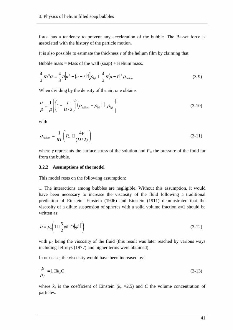
3. Physics of helium filled soap bubbles
41
force has a tendency to prevent any acceleration of the bubble. The Basset force is associated with the history of the particle motion.
It is also possible to estimate the thickness τ of the helium film by claiming that
Bubble mass = Mass of the wall (soap) + Helium mass.
( )[ ] ( ) heliumbfs aaaa ρτπρτπσπ 3333
3
4
3
4
3
4 −+−−= (3-9)
When dividing by the density of the air, one obtains
( )
+−
−= bfsbfsheliumDρρρτ
ρρσ 3
2/1
1 (3-10)
with
+= ∞ )2/(
41
DP
RThelium
γρ (3-11)
where γ represents the surface stress of the solution and P∞ the pressure of the fluid far from the bubble.
3.2.2 Assumptions of the model
This model rests on the following assumption:
1. The interactions among bubbles are negligible. Without this assumption, it would have been necessary to increase the viscosity of the fluid following a traditional prediction of Einstein: Einstein (1906) and Einstein (1911) demonstrated that the viscosity of a dilute suspension of spheres with a solid volume fraction φ«1 should be written as:
( )
++= 20 2
51 φφµµ O (3-12)
with µ0 being the viscosity of the fluid (this result was later reached by various ways including Jeffreys (1977) and higher terms were obtained).
In our case, the viscosity would have been increased by:
Ckef
+= 1µµ
(3-13)
where ke is the coefficient of Einstein (ke =2,5) and C the volume concentration of particles.

3. Physics of helium filled soap bubbles
42
2. The helium bubble reacts like a water bubble in the air and not like a bubble of air in water. In the latter case, it would have been necessary to change the value of ρ.
3. The bubbles remain spherical throughout their life. If the bubbles are deformed under the effect of strong pressure and acceleration gradients, then the expressions of the trail and the added mass are false, in particular for bubbles of which the density with respect to the flow is not neutral (most studies on accelerated particles deformation deal with air bubbles in water or water droplets in the air). Stokes (1851) showed that in the absence of inertia forces, the drag due to the flowing of a Newtonian fluid around a sphere is:
)(6 pf vvaDrag −−= πµ (3-14)
Barber and Emerson (2001) showed that a third of this force is due to the distribution of pressure around the sphere (drag due to the form), and the two remaining thirds to the friction against the wall of the sphere (drag due to friction). The Drag coefficient of the bubble can be derived by supposing that the drag is connected to the dynamic pressure and the apparent surface, as proposed by Schlichting (1968).
( )22
2
1pfD vvaCDrag −= ρπ (3-15)
From Eq. 3-14 and 3-15, one deduces the expression of CD :
)(
12
pfD vva
C−
=ρ
µ (3-16)
4. The flow is incompressible and irrotational, hence the fv2∇ terms disappear.
5. In the equation of the model Eq. 3-2, all the right-hand side terms are related to the slip velocity or to the slip acceleration, except for the forces of pressure and buoyancy. An important assumption of the model is that the slip between the bubble and the air is considered as negligible.
3.2.3 Conclusions on the theoretical model
Under the conditions of the assumptions above, the movement of a small particle in a flow depends primarily on the forces of pressure, inertia and gravitation.
For a particle with neutral density with respect to the fluid, mp = mf. In this case, pressure forces are balanced by inertia forces. Therefore, a neutral particle reliably follows the flow, provided the changes of properties of the fluid are negligible with respect to its diameter. For a particle lighter than the fluid, we have mp < mF. The bubble will tend to deviate and to be elevated from the real streamlines.
Therefore, it seems that more than the diameter of the bubble, the ratio (fluid density)/(bubble density) is the major parameter of the movement of the bubble.

3. Physics of helium filled soap bubbles
43
3.3 Experimental validation of Kerho and Bragg
Kerho and Bragg (1994) used a bubble generator of the same type as ours to test the aptitude of the bubbles to follow the flow. The experiment took place in a subsonic wind tunnel at the University of Illinois at Urbana-Champaign, Department of Aeronautical and Astronautical Engineering. Bubbles were introduced into a rectangular cross-section 90cm x 120cm tunnel containing a 53cm NACA 0012 airfoil. The light sheet was a 2mm thick laser plan and visualization was done thanks to a camera recording at the rate of 1000fps. A flow of 18m/s (Re = 640) was imposed in the wind tunnel. The result obtained while following about 50 bubbles is shown in Figure 3-3.
Figure 3-3 : Helium filled bubbles trajectories versus flow field streamlines (from Kehro and Bragg 1994)
One can notice that the trajectory of the bubbles deviates from the streamlines. The bubbles tend to cross the real streamlines and move upwards from the obstacle. No bubble cuts the flow downwards. One can thus conclude that the bubble generator produce either neutral bubbles or lighter-than-air bubbles, with a prevalence of lighter bubbles. This assumption is confirmed by the study of the bubble production process in a bubble generator. Within the “mini-vortex” filter (Anonymous 1988), only the bubbles which manage to follow the cyclonic movement of the air produced by the compressed air group make it outside of the generator. One can demonstrate that they have to be less heavy than the air:
Within the filter and for almost neutral bubbles, Eq. 3-2 is simplified into:

3. Physics of helium filled soap bubbles
44
pdt
dvp ∇=σ1
(3-17)
For an irrotational vortex,
avp π2
Γ= (3-18)
In addition, the equation of Bernoulli ensures that
−−= gh
vcsteP p
2
2
ρ (3-19)
From where
3
21
2 ap
Γ=∇π
ρ (3-20)
From where
3
21
2 adt
dvp
Γ=πσ
ρ (3-21)
For a mass of air moving around an irrotational vortex, the inertia due to centripetal acceleration balances the pressure forces and maintains the trajectory circular. The centrifugal acceleration produced by the vortex is written:
3
2221
2
1
2 aaaa
va p
c
Γ=
Γ==ππ (3-22)
From where finally,
cp a
dt
dv
σρ= (3-23)
The latter equation shows that
- If σ = ρ, inertia and centrifugal forces balance and the movement is circular.
- If σ > ρ, i.e. if the particle is heavier than the air, the centrifugal force prevails and the particle is crushed against the wall of the mini-vortex filter.
- If σ < ρ, inertia dominates and the particle is attracted towards the center of the mini-vortex without being destroyed and then goes up towards the outside with the neutral particles.

3. Physics of helium filled soap bubbles
45
Kerho and Bragg (1994) also built a numerical model based on the Eq. 3-2 in order to conduct a comparative study of the weight of the various terms in the equation. They showed in particular, that when approaching an obstacle under an angle initial of 0°, the bubbles move away from the obstacle if the pressure term is higher than the inertia term whereas they come closer to the obstacle in the opposite case.
By varying the density ratio σ/ρ and by comparing the trajectories obtained with real streamlines, they derived the error produced by non-neutral particles. For a density ratio of 0.8, which is 20% from neutral, they observed deviations of 12.8% to 17.7% for local gradients of pressures ranging respectively from 1.49Pa to 6.47Pa. On the other hand, a density ratio of 1.2, which is also 20% from neutral, gives a deviation between -13.6% and -10.4% respectively for the most and least severe pressure gradients. Last, for a given pressure gradient, the deviation was larger for a neutral bubble than for a heavier bubble.
They checked the fact that the ratio σ/ρ and the gradients of pressure in the flow are the dominant factors influencing the trajectory of a bubble. To a lesser extent, they observed that when the diameter of the bubble decreases, a smaller ratio of density makes it possible to follow the trajectory of the flow. In Eq. 3-2, when one decreases the diameter of the particle, the terms of pressure and inertia decrease proportionally to the radius cubed while the drag decreases only according to the radius squared. A lighter bubble is thus necessary to compensate for the increase in the relative weight of the drag term.
To conclude, commercial bubble generators destroy only bubbles that are heavier than air. Fortunately, most lighter than air particles go up and pop on the ceiling. When a bubble is neutral or lighter than air, its ability to follow the flow depends initially on the ratio σ/ρ and on the local gradients of pressure. In environments with weak gradients of pressure as is the case for free displacements in rooms, even not perfectly neutral particles follow the flow.
Making a particle visible depends on its own physical properties (size, light scattering ability) but also on the light source and the recording sensor. The next chapter explains the reasons of our choice for camera and illumination systems.
4. Choice of camera and light source
46
4 Choice of camera and light source
4.1 Camera requirements
Two main factors have to be taken into account when choosing a camera for flow visualization:
- The maximum frame rate: Frame rate is primarily chosen relatively to the maximum flow velocity. The quicker the flow, the higher the frame rate must be. In traditional PIV, time between two frames is calculated so that the fluid displacement is less than a quarter of the size of research windows:
max
max
V
dt
∆≤∆ (4-1)
where
4max
Ld =∆ (4-2)
with 22max yx ddd += (4-3)
where dx and dy are the pixel coordinates of the displacement on the image plane and L the pixel size of the research window. 3D PTV globally follows the same rule. For supersonic or highly turbulent flows, the frame rate must be over 1 KHz. In our case, maximum indoor speeds were found to be around 10m/s. Therefore, a 100fps camera allows restricting the inter frame real world displacement of a particle to less than 1cm.
Frame rate also has to be adjusted depending on the particles density in order to help minimize tracking ambiguities. So, the denser the seeding, the quicker the camera must be.
- The camera resolution: It is chosen depending on the size of the particles employed, the size of the field to be visualized (the larger it is, the higher the resolution must be), the illumination employed, and the background. Basically, particles must be seen. The field of observation of a sensor is given by Agui and Jimenez (1986):
Field of observation = Surface of the detector/M (4-4)
where M is the enlargement of the optical system. The diameter of a particle on the digital image is roughly given by the formula:
( ) 2/12222rdp dddMd ++=
(4-5)

4. Choice of camera and light source
47
with dp the real diameter of the particle, dr the size of the pixel or grain in the case of a photographic film, and dd the minimal diameter due to the refraction. dd is given by Adrian (1991):
( )MNOdd +⋅⋅⋅= 144,2 λ (4-6)
where NO is the aperture of the lens and λ the wavelength of the light used.
The observable depth of field where particles are seen accurately is given by Adrian (1991):
22 1
14
+⋅⋅⋅=M
NOz λδ (4-7)
Beyond the length δz, particles appear blurred. In the case of a traditional illumination by laser plan, δz is thus to compare with the thickness of the illuminated plan. A 2mm large particle seen with a 2000x2000 resolution sensor when using a 15mm focal length creates a 4 pixel large blob.
In a case of poor contrast with the background or when the light sheet is very large, sensors featuring a high number of gray levels should be preferred, typically at least 8 bits (which means 28 levels of gray). Lastly, a large size pixel offers a better sensitivity but a poorer resolution than a pixel of smaller size. Color images are generally useless in PTV. Our PTV experiments were never done on color images.
To conclude, tests in situ in presence of particles are always necessary before choosing the better camera. At the CETHIL, after testing we chose a 2352x1728-pixel, 30 to 300 fps, 8 to 10 bits sensor. Full details on camera hardware are given in Appendix A.
4.2 Light source requirements
Light source has to be strong and homogeneous enough for the cameras to see light reflected on tracers in every part of the measurement field. Especially in 3D PTV in large volumes, this must be true even for particles situated outside of the sensors object plane. Besides, the wavelength reemitted has to fit the spectral sensitivity of the recording sensor. Finally, light devices must produce low convective heat in order to keep the flow undisturbed. Unfortunately, pulsed lasers used in small scale PTV (Adrian 1991, Willneff 2002) cannot be used on larger volumes because the energy density of the light decreases rapidly when the beam is expanded.
In PTV as in PIV, the light sources can be either continuous or pulsed. In the latter case, they have to be synchronized with the cameras. After acquiring our camera system, we tested different light sources. Bubbles are not seen when using regular home light bulbs. When testing conventional stroboscopic light sources, we found that the light intensity

4. Choice of camera and light source
48
decreased rapidly when light frequency was increased. Helium filled bubbles could no longer be seen over about 50 Hz.
Sholzen and Moser (1996) used an arc lamp equipped with a cylindrical lens to create 2.5mx1.7mx0.12m large light sheet for helium filled bubbles visualization. Muller and Renz (1996) also used a cylindrical lens to expand the depth of a laser light sheet to a few centimeters. Machacek (2002) used 2000W regular halogen spot lamps to light up a 4mx2.1mx3m large wind tunnel. Sun and Zhang 2003 created a 5.5mx2.4mx0.065m large light sheet thanks to halogen lamps arranged vertically on the side of their test room. The total electrical power used was 7000W.
The selected light sources at the CETHIL are halogen lamps that produce 1000W power light each with very low convective heat generated thanks to fluorescent technology. Each lamp is equipped with eight mobile mirror reflectors and a tilted grid can be placed in front of the bulbs to uniformly diffuse light towards any chosen direction (see Figure 4-1). To further reduce heat generation, the lights sources were placed outside of the test room behind a glass panel whenever possible. Full details on the light sources are given in Appendix B.
Figure 4-1 : Continuous light source unit (without its grid-spot) used for indoor 3D PTV measurement in the test-room MINIBAT. Thermal Sciences Research Center of Lyon
(CETHIL), France
After choosing cameras and light sources, the next step is to build the correspondence between camera 2D image coordinates and object space 3D coordinates. This is camera calibration.

4. Choice of camera and light source
49
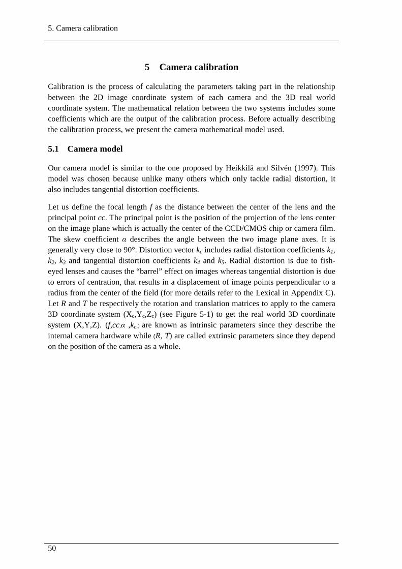
5. Camera calibration
50
5 Camera calibration
Calibration is the process of calculating the parameters taking part in the relationship between the 2D image coordinate system of each camera and the 3D real world coordinate system. The mathematical relation between the two systems includes some coefficients which are the output of the calibration process. Before actually describing the calibration process, we present the camera mathematical model used.
5.1 Camera model
Our camera model is similar to the one proposed by Heikkilä and Silvén (1997). This model was chosen because unlike many others which only tackle radial distortion, it also includes tangential distortion coefficients.
Let us define the focal length f as the distance between the center of the lens and the principal point cc. The principal point is the position of the projection of the lens center on the image plane which is actually the center of the CCD/CMOS chip or camera film. The skew coefficient α describes the angle between the two image plane axes. It is generally very close to 90°. Distortion vector kc includes radial distortion coefficients k1, k2, k3 and tangential distortion coefficients k4 and k5. Radial distortion is due to fish-eyed lenses and causes the “barrel” effect on images whereas tangential distortion is due to errors of centration, that results in a displacement of image points perpendicular to a radius from the center of the field (for more details refer to the Lexical in Appendix C). Let R and T be respectively the rotation and translation matrices to apply to the camera 3D coordinate system (Xc,Yc,Zc) (see Figure 5-1) to get the real world 3D coordinate system (X,Y,Z). (f,cc,α ,kc,) are known as intrinsic parameters since they describe the internal camera hardware while (R, T) are called extrinsic parameters since they depend on the position of the camera as a whole.
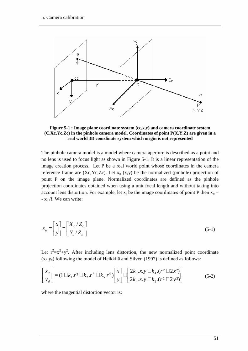
5. Camera calibration
51
Figure 5-1 : Image plane coordinate system (cc,x,y) and camera coordinate system (C,Xc,Yc,Zc) in the pinhole camera model. Coordinates of point P(X,Y,Z) are given in a
real world 3D coordinate system which origin is not represented
The pinhole camera model is a model where camera aperture is described as a point and no lens is used to focus light as shown in Figure 5-1. It is a linear representation of the image creation process. Let P be a real world point whose coordinates in the camera reference frame are (Xc,Yc,Zc). Let xn (x,y) be the normalized (pinhole) projection of point P on the image plane. Normalized coordinates are defined as the pinhole projection coordinates obtained when using a unit focal length and without taking into account lens distortion. For example, let xr be the image coordinates of point P then xn = - xr /f. We can write:
=
=
cc
ccn ZY
ZX
y
xx
/
/ (5-1)
Let r2=x2+y2. After including lens distortion, the new normalized point coordinate (xd,yd) following the model of Heikkilä and Silvén (1997) is defined as follows:
++++
+
+++=
²)2².(..2
²)2².(..2)..².1(
34
4365
421 yrkyxk
xrkyxk
y
xrkrkrk
y
x
d
d (5-2)
where the tangential distortion vector is:

5. Camera calibration
52
++
++=
²)2².(..2
²)2².(..2
34
43
yrkyxk
xrkyxkdx (5-3)
After applying the distortion, the final pixel coordinates xpixel of the projection of P on the image plane reads:
+++
=
=
22
11
.
)..(
ccyfc
ccyxfc
y
xx
d
dd
p
p
pixel
α
(5-4)
Eq. 5-4 can be rewritten as:
=
111
1
d
d
p
p
y
x
KKy
x
(5-5)
Where KK is called the camera matrix:
=100
0 22
111
ccfc
ccfcfc
KK
α (5-6)
This camera model is widely used in the computer vision community (Bouguet 2002, Favier and Dursapt 2005). The model can handle non-square CCD pixels thanks to the calculation of the aspect ratio fc2/fc1. This ratio must equal one whenever the pixels are square. The model can even handle non-rectangular pixels thanks to the calculation of the skew coefficient α. All those coefficient calculations are done through the calibration step.
5.2 Camera calibration
There are roughly two different camera calibration methods (Zhang 1999): Photogrammetric calibration and self-calibration. In photogrammetric calibration, a 3D object with precisely known features is observed. The calibration object generally consists of two or three perpendicular planes with square or round black and white patterns. Photogrammetric calibration can be done very accurately (Faugeras 1993) but requires a very precise and expensive calibration set-up.
Self-calibration doesn’t require any calibration object. The calibration parameters are derived (Hartley 1994, Luong and Faugeras 1997, Maybank and Faugeras 1992) by observing a static scene from a moving camera. Yet flexible, this method is not yet mature (Bougnoux 1998) and results obtained are not always reliable. Other calibration methods exist, including vanishing points for orthogonal directions (Caprile and Torre

5. Camera calibration
53
1990, Liebowitz and Zisserman 1998) and pure rotation calibration (Hartley 1994, Stein 1995).
The calibration technique used is halfway between photogrammetric calibration and self-calibration. Instead of a 3D calibration object, a 2D planar checkerboard is observed either by moving a camera or by moving the calibration board itself to at least two different locations. This technique was chosen because of its flexibility and its proven accuracy (Zhang 1999). Furthermore, its handling has been made easy thanks to its implementation in a Matlab toolbox by Bouyguet (2002.)
The calibration procedure can be described as follows:
1. Estimation of the planar homography between image plane and calibration target.
2. Estimation of all intrinsic parameters except distortion coefficients by using the orthogonality of vanishing points.
3. Estimation of extrinsic parameters.
4. Estimation of distortion coefficients following Heikkilä and Silvèn (1997) model.
5. Refining of all results by maximum likelihood estimation.
5.2.1 Estimating planar homography between camera image plane and calibration target
The camera model is first estimated without including distortion. Therefore, in the pinhole camera model, a point p(x,y) on the image plane is related to a 3D point P(X,Y,Z) by the matrix relation as shown in Section 5.1:
[ ]PTRKKps =. (5-7)
where s is a scale factor, and by abuse of language, p=[x,y,1]T and P=[X,Y,Z,1]T. On the calibration target, we assume Z=0. Therefore, r i being the i th columns of R,
[ ] [ ] PHY
X
TrrKKY
X
TrrrKKy
x
s~
11
01
. 21321 =
⋅⋅=
⋅⋅=
(5-8)
Eq. 5-8 shows that p and P are related by a homography noted H. H can be regarded as a bijective operator that changes coordinate frames, as shown in Figure 5-2. For each

5. Camera calibration
54
pixel coordinates p corresponds a unique point P on a given target plane which verifies P=Hp and p=H-1P.
Figure 5-2 : Homography between image plane and calibration target (for the sake of convenience, the optical center C of the system is placed behind the image plane)
H is a 3x3 matrix estimated by a maximum likelihood method. Assuming that the relationship between the marker points Pi on the calibration target and their respective 2D images pi is corrupted by a Gaussian noise of mean 0 and of covariance matrix Λpi, the following relation is minimized to obtain the columns hi of H:
)ˆ()ˆ( 1ii
im
Tii pppp
i−Λ−∑ − (5-9)
where
=
iT
iT
iTi
Ph
Ph
Php
2
1
3
1ˆ (5-10)
All points being extracted independently using the same procedure, value of Λpi is generally assumed to be σ2I where σ is the standard deviation. Eq. 5-9 thus becomes a non-linear least square minimization problem which is resolved with a Levenberg-Marquardt algorithm as presented by More (1977). The way of finding the initial guess required by the algorithm is presented by Zhang (1999).
5.2.2 Estimating intrinsic parameters by using the orthogonality of vanishing points
First, let us define key words used in projective geometry. An ideal point is a point where parallel lines meet at infinity, just as two railways meet when fading away in the horizon. A vanishing point is the image of an ideal point on the camera image plane. Practically, it is the image of the ideal point created by parallel lines of the calibration
5. Camera calibration
55
target after applying the homography H-1 (see Figure 5-2). A set of ideal points forms an ideal line.
An important result from projective geometry is that the corresponding vanishing line can be obtained by applying HT to the ideal line (see Semple and Kneebone 1952 for demonstration). Another standard result is that the line going through the focal point C and a vanishing point is parallel to the set of lines that gave rise to the corresponding ideal point (see Figure 5-3).
Figure 5-3 : Ideal and vanishing points and lines
The coordinates of the principal point are first determined. Figure 5-3 shows a case where vanishing points are seen on the image plane. However, in most actual cases, vanishing points are found outside of the physical image. Actually, they are found at infinity on the image plane. Therefore, the calculation of the principal points is done by the following procedure, as described by Beardsley and Murray (1992):
- HT is applied on the coordinates of the ideal line to obtain the coordinates of the vanishing line L.
- The vanishing point V1 is calculated as the intersection between L and the ideal line.
- 3D coordinates of the corresponding ideal point I1 are calculated by I1=H V1.

5. Camera calibration
56
- 3D coordinates of I2 are calculated using the constraint that I1 and I2 are associated to perpendicular directions on the projective plane. For example, an ideal point I1(a,b,0) gives an opposed ideal point I2(-b,a,0).
- 2D coordinates of V2 are calculated by V2=H-1I2.
Finding the principal point rests on the important property that is the line perpendicular to L at point V2 passes through the principal point P (see Beardsley and Murray 1992 for the proof). Therefore, applying the above mentioned procedure for at least two positions of the calibration target yields the position of the point principal point as the intersection of the lines passing through V2.
If the aspect ratio has not been corrected before starting the procedure, the line through V2 and the principal point cannot be perpendicular to L since perpendicularity is not preserved under changes of aspect ratio. The aspect ratio is changed iteratively, starting from a probable value (for example the one given by the camera manufacturer) until the lines through V2 are close to concurrency. The concurrent point of constraint lines can be found using orthogonal regression. The process yields the aspect ratio.
To calculate the focal length, one additional vanishing point V3 on L has to be found. V3 is such that the angle V2CV3 is 45° as shown in Figure 5-4. V3 is found the same way as V2: V2 is used to compute the ideal point I2. I2 is used to compute the ideal point I3 with the constraint that the angle between the two directions is 45°. Then I3 is used to compute V3. Simple trigonometry shows that distance CV2 is equal to distance V2V3, the latter being known. Then the focal length CQ is computed as a side of the right-angle triangle CQV2 which sides CV2 and QV2 are already known.
Figure 5-4 : An additional vanishing point V3 is computed to find the focal length
An experimental example and a discussion on the accuracy of this way of computing intrinsic parameters are found in Beardsley and Murray (1992).

5. Camera calibration
57
5.2.3 Estimating extrinsic parameters
Eq. 1-8 defines H up to a scale factor λ:
[ ] [ ]TrrKKhhhH 21321 ⋅== λ (5-11)
Once H is known, the computation of extrinsic parameters is straightforward:
31
21321
211
1 ;;; hKKTrrrhKKrhKKr −−− =×=== λλλ (5-12)
where
21
11
11
hKKhKK −−==λ (5-13)
Because of experimental and computational approximation, R has to be fitted to fulfill the requirements of a rotation matrix. Estimating the best rotation matrix from a 3x3 matrix is done by minimizing the Frobenius norm of the difference R-Q as shown in Zhang (1998).
5.2.4 Estimating distortion coefficients
Following Heikkilä and Silvén (1997) model, Eq. 5-2 can be rewritten as:
−−
=
++
yy
xx
k
k
k
k
k
yrxyyryryr
xrxrxyxrxr
d
d
5
4
3
2
1
62242
62242
22
22 (5-14)
where xd and yd are the distorted pixel coordinates that can be computed from pixel coordinates using Eq. 5-4, and (x,y) are distortion-free normalized (pinhole) coordinates. Unknowns coefficients (k1,k2,k3,k4,k5) are found by using a least squares method from at least three different points.
5.2.5 Final maximum likelihood estimation
The purpose of this step is to refine all the parameters found using experimental calibration data. The method used is the same as Zhang 1999. The following functional is minimized:
( )2
1 154321 ,,,,,,,,~∑∑
= =
−n
i
m
jjiiijij PTRkkkkkKKpp (5-15)

5. Camera calibration
58
where m is the number of calibration points, n the number of images, and
( )jiiij PTRkkkkkKKp ,,,,,,,,~54321 the projection of point Pj of image i according to Eq.
5-8 followed by distortion and pi its pixel image. This non-linear minimization problem is also solved with a Levenberg-Marquardt algorithm implemented in More (1977). Initial guesses required by the algorithm are provided by using the results of the previous sub-sections (some parameters like skewness and distortion can be set to 0 as an initial guess). Rotation R is parameterized by a 3x1 vector obtained by applying the Rodrigues formula presented in Faugeras (1993).
5.3 Multi-camera calibration
The procedure described in sections 5.2.1 to 5.2.5 is repeated for each camera separately. Intrinsic parameters yielded by the process are kept. Then, correspondence to the common 3D coordinate system is calculated by recomputing the extrinsic parameters of all cameras from a single position of the calibration target as shown in Figure 5-5.
Figure 5-5 : The calibration target must be viewed simultaneously by all cameras when computing the common real world reference frame

5. Camera calibration
59
After calibration, the cameras must not be moved during the whole recording session. This would cause a change in the value of the extrinsic parameters. It is worth noticing that calibration can also be made after recording particle images, provided the cameras are not moved.
After flow recording, the images are supplied to the tracking algorithm which proceeds to the particle detection step.

6. Particle detection
60
6 Particle detection
The aim of the particle detection procedure is to compute the pixel coordinates of each particle center. Unlike traditional 3DPTV, PTV algorithm for large volumes must include a step where oversized particles are removed from the images. Those over large speckles are created by images of particles getting close to the cameras, since particles are not constrained to remain inside a small delimited volume. Particles creating those blobs are generally out of the common field of vision. The particle detection process includes the following steps:
1. Creation and subtraction of background from images. 2. Removal of noise and over large particle images. 3. Calculation of pixel coordinates.
6.1 Creation and subtraction of background
The purpose of this step is to feed the tracking algorithm with grey level images of particles over a totally black background. Creation of the background is generally made by averaging a certain amount of images. Averaging the background is used to cope with the variations of continuous light intensity. It can be made in the presence of particles but conducting this process before introducing particles (or after all particles are gone) gives better subtraction results.
When averaging the background in the presence of particles, it is worth averaging the whole set of particle images to be treated by the tracking algorithm. When averaging without particles, one should not use more than about 10 images otherwise the resulting image gradually becomes saturated. After being created, the background is subtracted from each image. However, the result of the process generally does not permit separation of particles from residual noise.
6.2 Removal of noise and over large particles images
The main image processing functions usually used to get clear images of particles are:
- Contrast enhancement: This step is not compulsory, depending on the quality of the particle images. It can be performed efficiently by high-pass filtering to suppress the variations of background level due to noise and light intensity variations.
- Thresholding: This operation consists in retaining only the pixels which luminance is above a certain value determined empirically. Since noise has generally a luminance lower than particles, thresholding permits getting good images of particles. Finding the appropriate threshold was made experimentally (the operation is rather quick) but it can also be implemented automatically for instance by minimizing the interclass-variance of the segmented black and white pixels (Otsu 1979).

6. Particle detection
61
- Removal of isolated pixels: Helium filled soap bubbles generally cover more than one pixel. Typically they create speckles of diameter three to six pixels. Therefore, isolated pixels can more than often be assimilated to remaining noise. They can be removed by eroding the image with structuring elements of 2-pixel lengths.
Figure 6-1 : Particle image before and after background and noise removal (the processed image is inverted for better clarity)
The above list is not exhaustive. We only mentioned the operations that worked best when dealing with helium filled bubbles as shown in Figure 6-1. Depending on the images quality, one may need to use additional image processing operations such as image filtering to enhance contrast.
As previously said, whenever the cameras are situated in the same room as the seeded flow, some over large speckles may be created by images of particles getting close to the cameras (see Figure 6-2). Removing blobs of a certain diameter from an image is a standard procedure in image processing called opening.
An opening is an erosion followed by a dilation using the same structuring element for both operations. However, this operation generally gives poor results with images of helium filled bubbles. Since the particle images are neither perfectly round nor perfectly filled, the bubble shells can generally be seen after the processing (see Figure 6-3).
After removing the averaged background, images of overlarge helium filled bubbles can be removed efficiently by the following procedure:
- Binarize the image. The binary threshold level can be assigned empirically, or automatically calculated from iterative algorithms (Otsu 1979, Crouser et al 1997).

6. Particle detection
62
- Fill-up and bridge all particle images in order to get homogeneous blobs (see Figure 6-4a). This filling-up and bridging may be made by iteratively dilating the image with structuring elements [1,1] and [1,1]T.
- Erode the output image with a square structuring element of size the maximum diameter of a particle in the common camera’s field of vision (see Figure 6-4b). Here particles of diameter equal or less than the maximum allowed are removed from the image. This maximum diameter value is determined empirically.
- Dilate the resulting image with a square structuring element larger than the one previously used. Good results were achieved with a structuring element twice the size of the first one used (see Figure 6-4c).
- Subtract the output image from the original unbinarized particle image (image before applying the first step of the procedure) to keep the Gaussian profile of the bubble images. The resulting image only contains particles of diameter equal or less than the size of the structuring element in step 3 (see figure 6-5).
(a) (b)
Figure 6-2 : (a) Binarized particle image before blob removal (the image is inverted for clarity) . (b) Standard over-large particle (blob). Blobs create many centroids leading to
false detections

6. Particle detection
63
Figure 6-3 : Over-large particle image after standard image opening with an 8-pixel large disk-shaped structuring element. Bubble’s shell is still visible
(a) (b) (c)
Figure 6-4 : Proposed procedure for blob removal: (a) Blob filled and bridged. The displayed blob covers a 28x27 pixel region. (b) Same blob after an erosion with an 8-pixel
square-shaped structuring element (16x15 pixel region). (c) Same blob after dilatation with a 16-pixel square-shaped structuring element (31x30 pixel region)
Figure 6-5 : Example of output image after the blob removal procedure. The image only contains particles of diameter less than 9 pixels

6. Particle detection
64
6.3 Calculation of particle centers pixel coordinates
Most particles center detection methods found in literature attempt dissociating individual particles form overlapping particles images. Template matching (Gruen and Baltsavias 1988, Guezennec et al. 1994) gives poor results with soap bubbles because of the wide range of particle shapes and sizes after image processing. Hough transform (Hough, 1962) is ill-adapted to the smallness of the pixel area covered by average particles which varies from 2x2 to 8x8 pixels, depending on the distance from the cameras. Invariant second order grey moments method (Teh and Chin, 1988) works well when only two particle images are overlapping but fail when three particles create a larger speckle. Higher order moments are very noise sensitive. 2D Gaussian fitting (Mann et al. 1999, Nobach and Honkanen 2005) works well when particles intensity profile can be approximated by a Gaussian. In our case, a single particle often features two intensity peaks. In addition, Gaussian fitting is computationally costly and gives better results on large particle images. The same drawbacks work for neural network methods (Carosone et al. 1995) though those methods are robust in case of noisy images.
As shown in Section 3.1, particles are seen as two (or only one) bright spots on the particle shell symmetric relative to the center of the sphere (see Figure 3-1). This fact makes relevant the use of weight averaged methods to calculate the center of mass of each particle. For each particle, the coordinates (xc,yc) of the center or mass are given by:
∑∑=
),(
),(
yxI
yxxIxc
;
∑∑=
),(
),(
yxI
yxyIyc
(6-1)
where (x,y) are the pixel coordinates of each pixel belonging to the particle and I(x,y) the pixel luminance.
This method also used by Machacek (2003) allows recognizing two connected bright spots as a single particle. Unfortunately, although weight averaging has some overlapping handling capabilities, two centroids are generally created whenever the two bright spots are not connected as shown in Figure 6-6. We deliberately chose not to bridge those particles by applying a one or two pixel dilatation. Such an operation would have resulted in reducing the spatial resolution of the overall 3D tracking by making partially overlapping or very close particles appear as a unique particle.

6. Particle detection
65
Figure 6-6 : Output of the center of mass calculation by weight averaging on three particles of the same image. Far left and center particles yield one centroid whereas far
right particle displays two disconnected local maximum and therefore yields two centroids
As shown be Ouellette et al. (2006), the weight averaging method may be less accurate than Gaussian fitting and neural network methods whenever particles are far enough from the camera to feature a single local maximum. Nevertheless, this method is efficient, readily implemented and rapid. Particle centers are given with sub-pixel accuracy (down to 1e-01) with derisive computation time. Furthermore, in large volumes (over 1m3), overlapping cases where estimated to less than 5% of particle images for camera resolutions over 1024x1024 pixels.
Once we can accurately detect particle centers on each image, the next step is to establish their 2D trajectory from successive images. That is temporal tracking.

7. Temporal tracking
66
7 Temporal tracking
Temporal tracking is the research of particle trajectories on successive 2D particle images. There is no attempt to match particles in 3D (unless needed to resolve ambiguities) at this time of the process. Therefore, temporal tracking can be made separately, one camera at a time.
7.1 Existing heuristics
Tracking many particles over many time frames is known to be a NP-hard problem
(Veenman et al. 2003). Therefore, only a few frames at a time are used to solve the ambiguities. Traditional temporal tracking heuristics include nearest neighbor heuristic, 3-frame minimum acceleration heuristic and 4-frame minimum changes in acceleration heuristic. Most of these methods proceed in two steps. First, the center of a search region is calculated using a constraint on velocity or acceleration. Then, all particles within the search region are tested using a cost function that has to be minimized. Depending on the heuristic, the cost function accounts for constraints on the amplitude and direction of velocity or acceleration.
- Nearest neighbor heuristic: Particle i at instant n is linked with particle j at instant n+1 which is closest to the position xi
n+1. Therefore, the following cost function is minimized:
ni
nj
nij xx −= +1φ (7-1)
This is the simplest, but also the less accurate tracking scheme.
- 3-frame minimum acceleration heuristic: The center of the search region is calculated assuming a somewhat constant velocity over three consecutive frames:
11 2 −+ −=∆+= ni
ni
ni
ni
ni xxtuxx (7-2)
Then in the cost function applied to particles falling inside the search region can be:
2
11
)(2
2
t
xxx ni
ni
njn
ij ∆
+−=
−+
φ (Malik et al. 1993; Dracos 1996) (7-3)
Or

7. Temporal tracking
67
+
⋅−+
⋅
⋅−=
+−
+−
+−
+−
11
11
211
11
1 211nk
ni
ni
nj
nk
ni
ni
nj
nk
ni
ni
nj
nk
ni
ni
njn
ijkxxxx
xxxxw
xxxx
xxxxwφ (7-4)
(Chetverikov and Verestoy 1998)
where w1 and w2 are weights (w1 =0.1, w2 =0.9) which penalize respectively changes in velocity direction and velocity magnitude.
- The 4-frame minimum changes in acceleration heuristic: The center of the search region is determined as in the 3-frame minimum acceleration scheme. However, for each particle in the search region at instant n+1, a second search region is created at frame n+2 using:
( ) ( )22 22 tatuxx ni
ni
ni
ni ∆+∆+=+ (7-5)
Then the cost function can be:
2
1112
)(2
22
t
xxxxxx ni
ni
nj
ni
nj
njn
ij ∆
+−−+−=
−+++
φ (Malik et al. 1993, Dracos 1996)
(7-6) Or
22 ++ −= ni
nj
nij xxφ (Ouellette et al 2006) (7-7)
It is important to note that the estimation of the search region center can be made either in 2D image space or in 3D object space. The latter scheme generally permits avoiding ambiguities caused by particles with equal cost functions, especially in case of overlapping particles.
Two novel particle tracking schemes where developed at the CETHIL and at the University of Illinois at Urbana-Champaign, Department of Agricultural and Biological Engineering, Bioenvironmental Engineering Laboratory.
- Temporal tracking by modified fast normalized cross-correlation.
- Temporal tracking by polynomial regression.

7. Temporal tracking
68
7.2 Modified fast normalized cross-correlation tracking
7.2.1 The algorithm
This temporal tracking method is partly inspired from traditional PIV cross-correlation methods. However, instead of looking at the next frame for a pattern composed of a group of particles, the pattern is a single particle. Besides, there is a procedure to solve ambiguities. The template matching criteria taken into account are size, shape and luminance of the particle.
The implementation of normalized cross-correlation follows the formula from Lewis (1995):
( )[ ] ( )[ ]( )[ ] ( )[ ]∑ ∑ −−−−
−−−−=
yx yxvu
vu
tvyuxtfyxf
tvyuxtfyxfvu
,
2
,
2
,
,
,,
,,),(γ (7-8)
where f is the research window, t is the mean of the template (interrogation window)
and vuf , is the mean of f(x,y) in the region under the template. Cross-correlation is done
in the spatial or frequency domain, depending on the size of particles. Local sums are first pre-computed. Then they are used to normalize the cross-correlation function and get correlation coefficients.
Tracking ambiguities arise when there are more than one correlation peak. The ambiguity solving procedure is launched whenever the difference between the two maximum cross-correlation coefficients is less than 10%. Ambiguities solving is done by the Lagrangian extrapolation of an estimate position using the last three positions of the particle or last two, when ambiguity solving is needed at the third frame:
cbtatxn ++=+2
1 (7-9)
where xn+1 is the estimate position, t the frame number, and a,b,c the coefficients determined by polynomial curve fitting in a least square sense. The physical meaning of the extrapolation is a minimization of changes in particle acceleration. The particle closest to the estimated position is chosen. Finding the estimate position can be done either in 2D space or in 3D space, provided 3D matching of particles has already been done.
The main inputs of the temporal tracking algorithm are the size of the interrogation window and the size of the research window. The templates (interrogation windows) sampled at instant t consist of square matrices framing each bubble. The pixel length of those matrices is 2r where r is the maximum pixel radius of a bubble. The research windows sampled on image at instant t+1 consist of a matrices centered on the previous location of the bubble at instant t. The length of each research window must include the

7. Temporal tracking
69
maximum possible displacement of a particle between two frames. It can be quickly chosen by visually inspecting the flow. Its radius α can also be computed by:
rn
tV+=
.maxα (7-10)
where Vmax is the estimated maximum velocity of a bubble, t the time interval between two successive images, n the pixel length (m/pixel).
In order to account for changes in particle image size due to motion in large volume and particle speed due to the characteristics of the flow, interrogation and research windows are deformable.
This method heavily relies upon the high speed of cameras. If the particle goes out of the research window, a correlation peak will be found. The detailed procedure of this temporal tracking scheme is as follows:
1. On the first image, frame each particle with a matrix whose size is the average size of particles in the common field of vision. If some particles do not fit in the frame, those interrogation windows may grow up to the maximum size allowed for a particle in the common field of vision.
2. On the second image, create matrices centered on the previous location of bubbles at first image. Size of those matrices is the maximum allowable displacement between two frames. However, if there is no particle framed into those research windows, they iteratively grow up to 1.5 of the maximum allowed displacement.
3. Apply fast normalized cross-correlation.
4. In order to avoid the “slipping” effect of a particle progressively going out of the template, recompute the centroid of the candidate particle and go back to step 1 starting from the second image. Use first order polynomial approximation to solve ambiguities in frame Three and second order polynomial approximation to solve ambiguities from fourth frame on.
7.2.2 Validation
Validation of the modified normalized fast cross-correlation has been done using both simulated and experimental data. Four indexes were used to assess temporal tracking efficiency:
- The “tracking density” ratio ξ measures the ratio of mean particle spacing (in a nearest neighbor sense) to mean displacement of particles between two consecutive frames. It is an indicator of the tracking difficulty (Malik et al. 1993).

7. Temporal tracking
70
- The “correct tracking” ratio γ2D is the number of tracked positions which are identical to input particle positions from the simulation tool divided by the total number of tracked positions. This ratio only deals with tracked trajectories. It is an indicator of the tracking accuracy (Li 2008).
- The “tracking efficiency” ratio E2Dtrack (Malik et al. 1993) is the number of correctly tracked 2D trajectories divided by the total number of trajectories. This ratio deals with all trajectories. It is an indicator of the overall tracking efficiency.
- The maximum number of tracked particles in 2D space. It is a standard indicator of tracking limits.
For the last three indexes, we consider a tracked position “correct” when it is either identical to the actual particle position or its deviation from the latter position is less than the radius of the particle. This condition physically means that the tracked centroid is “inside” the actual particle.
7.2.3 Validation based on simulation data
Simulated particle images where generated by our particle images generation tool described in Appendix D. Our simulation tool in its temporal tracking assessment part works as follow: First a set of particles is created with chosen density and number but random positioning in 2D image space. Particles are disk or square shaped white patterns in 3x3 matrices with random luminance. Images consist of black matrices of chosen rectangular size and resolution where particles are generated. Several types of noise can be added to the resulting images (see Appendix D). Second, all the particles are given a linear or helix 2D displacement of chosen inter frame pixel displacement. The resulting images are fed as input of the temporal tracking algorithm and tracked positions are compared to virtual input positions.
n particles were given a linear displacement over ten frames with a three pixels per frame displacement. Virtual image resolution was 2000 x 2000 pixels and no noise was added. The initial size of the interrogation windows was set to three while the initial size of the research windows was set to six. For each value of n, indexes ξ, γ2D and elapsed CPU time were calculated and are shown in Table 7-1.
n 20 30 60 120 240 480 960 1920 3840
ξ 75,7 62,1 40,5 30,2 22,3 16,4 10,8 7,77 5,63
γ2D 0,99 0,95 0,94 0,925 0,89 0,82 0,7 0,6 0,55
CPU time
(s) 3,6 5,3 10,6 17 33 59,5 111,3 179,7 310
Table 7-1 : Temporal tracking performances of the modified normalized fast cross-correlation scheme

7. Temporal tracking
71
Graphs of tracking density and number of particles versus “correct tracking” ratio γ2D and CPU elapsed time were also drawn. Results show that the algorithm performs extremely well up to 240 particle images. Then performances gently decrease as shown in Figure 7-1 and Figure 7-2 but remain over 50% even for dense particle images (γ2D = 0.55 for n=13840 and ξ < 5.63. This tracking density ratio was calculated over the whole domain of the image. On certain image regions, ξ was 2.5. All particles were tracked.
The performances shown in Table 7-1 have to be decreased by 20% when the particle linear trajectories are crossing each other.
Figure 7-1 : Number of particles vs. correct tracking index for the modified normalized fast cross-correlation scheme
Figure 7-2 : Tracking density index vs. correct tracking index for the modified normalized fast cross-correlation scheme

7. Temporal tracking
72
By drawing tracked positions on the same figure as input particle trajectories, the tracking accuracy can be visually assessed, as shown in Figure 7-3.
Temporal tracking by fast normalized cross-correlation is quicker than most other tracking heuristics. The elapsed CPU time is quasi proportional to the number of particles for fixed trajectory lengths as shown in Figure 7-4.
Figure 7-3 : Temporal tracking of 240 particles on 10 frames by the modified fast normalized cross-correlation scheme. Blue crosses represent tracked positions while white
tracks represent actual input trajectories (zoomed-in image)
Figure 7-4 : CPU elapsed time vs. correct tracking index for the modified normalized fast cross-correlation scheme

7. Temporal tracking
73
The decrease in the algorithm performances is strong when the trajectory length increases beyond 10 frames. With n=960 and ξ =10.8, we found γ2D = 0.56 for a 15-frame long trajectory and γ2D = 0.46 for a 20-frame long trajectory. This time-dependant instability does not depend on the implementation hardware. The same drawback was observed when trying to implement fast normalized cross-correlation on graphic processor units (GPU). It was observed that the first ten frames are correctly tracked and then the tracking becomes erroneous on certain trajectories as shown in Figure 7-5.
Figure 7-5 : Temporal instability of the modified fast normalized cross-correlation scheme. Blue crosses in the zoomed image represent tracked positions while white tracks
represent actual input trajectories. n=960, trajectory length=20 frames, γ2D = 0.46
The elapsed CPU time for temporal tracking is also more sensitive to trajectory length than to the number of particles. It was found that for 960 particles, the CPU time was 111.26s over 10 frames, 246s over 15 frames and 398.3s over 20 frames.
7.2.4 Validation based on experimental data
Modified fast normalized cross-correlation was also validated using experimental data. Helium filled soap bubbles were emitted in the 3.1mx3.1mx2.5m high test-room MINIBAT of the Thermal Sciences Research Center of Lyon (CETHIL). For density ξ =42.9 and n=51, tracking yielded γ2D = 0.8 and E2Dtrack=0.72. Five trajectories were not tracked at all as shown in Figure 7-6.
To conclude, modified fast normalized cross-correlation is suited to temporal tracking of dense particle images provided trajectory length does not exceed 10 to 15 frames.

7. Temporal tracking
74
Figure 7-6 : Tracking of real bubbles with the modified fast normalized cross-correlation scheme. Blue crosses represent tracked positions while white tracks represent actual input
trajectories
7.3 Temporal tracking by polynomial regression
7.3.1 The algorithm
This tracking scheme utilizes a second order polynomial regression method to predict the center of the search region:
cbtatx iii ++= 2
(7-11)
where xi stands for the pixel coordinates vector and i for as much as five previously linked trajectories not necessarily on consecutive frames. Constants a, b, and c are acquired by least square fitting. As previously said, the physical meaning of the regression is also aimed at minimizing the change in the particle acceleration.
The cost function used to resolve conflicts within the search area is:
∑
∑
=
=−−
=3
0
2
3
0
2
k k
k kk
D
HGD τφ
(7-12)
where Dk is the particle displacement between previously linked frames k and k+1:

7. Temporal tracking
75
1+−= kkk xxD (7-13)
Let τk be the half time between frames k and k+1, and G and H the constant vectors resulting from the linear regression of order 1 fitting D over frames 0 to 3:
HGD kk += τ (7-14)
The cost function thus appears as a regression residual normalized by a geometrical mean displacement. Its physical meaning is also to minimize the changes in particle acceleration since linear regression of Eq. (7-14 assumes zero acceleration.
The radius of the search area reads:
( )21
21111 tt
xxttr nn −
−−= ++ α (7-15)
where α is a preset parameter, ti and xi respectively time and position at linked frame i.
The tracking scheme includes four additional features. First, a “cross-gap” strategy accounts for particles undetected in a single frame. Whenever a particle is absent from the search region at frame n+1, the regression and the search is extended to frame n+2 and the trajectory goes on if a suitable particle is found. If a suitable particle is not found, the trajectory is ended. Second, recomputing particles centroids at each frame (instead of doing it once and tracking them in 2D space) allows starting new trajectories for new particles entering the field of vision. Third, a false trajectory detection step only keeps the longest one of two trajectories having the same coordinates. This is done to compensate for the extra trajectories created by the previous step. Finally, particles shared by two trajectories are removed. Let Te be a trajectory ending at frame t and Ts a trajectory starting at frame t or t+1. The cost function of a new trajectory composed of the last three positions of Te and first three positions of Ts is calculated according to Eq. 7-12. If the cost function is less than a preset parameter β (around 0.2), the bridge is validated. This tracking strategy is designed to yield longer trajectories than traditional ones (Li 2008).
Going through this process with a spatial matching at each time step would have been computationally costly and error prone. As will be shown in Section 8, doing temporal tracking first also allows us to check the 3D matching several times throughout the trajectory. This is why temporal tracking is done before spatial matching.
7.3.2 Validation
The polynomial regression scheme was validated using simulation data from Okamoto et al. (2000). The 2D displacement of a jet flow impinging on a wall was observed over 90 frames on 256x256 pixel images. Tracking difficulty index ξ was 3.4 over the

7. Temporal tracking
76
domain of the whole image. Mean length of trajectories yielded was 37 frames on noiseless images and 32 frames on noisy images. E2Dtrack was around 0.95 and γ2D was always over 0.97 which means that long input trajectories were broken into several correctly tracked shorter trajectories.
The algorithm was compared to a three frames minimum acceleration scheme (Eq. 7-3) with a nearest neighbor cost function (Eq. 7-1). It was shown that, thanks to its gap-crossing strategy, the algorithm yields longer trajectories and is more robust against noise than the described scheme. Full details on validation are given in Li (2008.) However, the computational time of the polynomial regression scheme is higher than that of traditional schemes since more operations are done.
7.4 Comparison
The polynomial regression and modified fast normalized cross-correlation heuristics were compared using simulated and experimental data. First, using our particles simulation tool, 960 particles were given a three pixel per frame linear displacement over 20 frames. Image resolution was 2000x2000 pixels. Tracking difficulty was ξ≈10.8 over the whole image domain. As previously indicated, the size of interrogation windows was three while the size of research windows was six. Temporal tracking by modified normalized cross-correlation yielded γ2D = 0.46, E2D=0.46 as shown in Figure 7-5 while temporal tracking by polynomial regression yielded γ2D = 0.97, E2D=0.96 as show in Figure 7-7. Computational time was 398.3s for the cross-correlation scheme and 406.8s for the polynomial regression scheme.
Figure 7-7 : Red crosses in the zoomed image represent tracked positions using temporal tracking by polynomial regression while white tracks represent actual input trajectories.

7. Temporal tracking
77
n=960, trajectory length=20 frames, γ2D = 0.97, E2D=0.96. This figure is to be compared with Figure 7-5
Secondly, 2D trajectories of helium filled bubbles moving over a heater (see full details on that experiment in Section 10-3) were calculated using both methods. Trajectory length was only six frames. For both methods, initial interrogation windows were 6-pixel sized and research windows 10-pixel sized. The modified cross-correlation scheme gave better results as shown in Figure 7-8. It shows that the polynomial regression tracking scheme needs at least six frames to better reject false candidate trajectories.
(a)
(b)

7. Temporal tracking
78
(c)
(d)
Figure 7-8 : Polynomial regression scheme (a,c) vs modified cross-correlation scheme (b,d) over six frames of real bubbles displacement. Comparison of real and tracked trajectories
shows a better coverage of the cross-correlation scheme
To conclude, we can say that the modified cross-correlation scheme features higher performances for trajectories that are less than 10 frames. Beyond 10 frames, cross-correlation becomes instable, probably due to the very small pixel area covered by the tracked patterns (as suggested by Maas et al. 1993) and temporal tracking by

7. Temporal tracking
79
polynomial regression yields less numerous but more accurate trajectories. This latter fact was also confirmed by experimental data (see Section 10).
Once trajectories have been found on each camera images sequence, they have to be 3D matched before calculating final 3D coordinates. That is the purpose of the 3D reconstruction step.

8. 3D reconstruction
80
8 3D reconstruction
8.1 Correspondence problem
This section presents the method used to 3D match the trajectories provided by the temporal matching step. The correspondence problem (also called spatial matching problem) can be enunciated as follows: All the particles are exactly the same and there is no physical characteristic to identify each of them. Therefore, how can we identify a particular particle or a particle trajectory among hundreds of similar particles in a seeded area viewed by three cameras at the same time? Two strategies to solve the correspondence problem will be presented here.
8.1.1 Using the epipolar constraint
This is a standard and well known method (Maas 1992). For convenience, we used the camera pinhole model (see Section 5.1). The epipolar geometry with two viewpoints is described in Figure 8.1. The epipolar constraint can be enunciated as follows: If the pixel image p1 of a real point P is known on one camera, the image p2 of the same point on the second camera image plane must lie on a line called the epipolar line (p2,e2) where e2 is where camera 1 is seen from camera 2; e2 is called an epipole. The correspondence between p1 and the epipolar line (p2,e2) is described by the fundamental matrix F12:
0~~2121 =pFpT (8-1)
where 1~p and 2
~p are normalized (pinhole) pixel coordinates of p1 and p2 with a third
coordinate equal to 1 (see Eq. 8-5).
Figure 8-1 : Epipolar geometry with two viewpoints. The image of P
must lie on epipolar lines (p1,e1) and (p2,e2)

8. 3D reconstruction
81
Epipolar lines are the traces of the plane (C1,P,C2) on each camera image plane and all epipolar lines on camera i cross the epipole ei. When using three or four cameras, ambiguities in the spatial matching on a camera image plane are lifted by the intersection of epipolar lines, as shown in Figure 8-2.
Our implemented spatial matching procedure is as follows:
First, the fundamental matrix of each pair of cameras is calculated. For two cameras 1 and 2, the fundamental matrix reads:
[ ] TT RRTRRTF 21221112 ⋅⋅⋅−= × (8-2)
with Ti and Ri respectively the 3x1 translation vector and the 3x3 rotation vector which transform camera i 3D coordinates system XXc into the calibration target 3D coordinates system XX:
TXXRXXc +⋅= (8-3)
Figure 8-2 : Epipolar geometry with three viewpoints. Matching ambiguities in the determination of the image of P are lifted by the intersection of epipolar lines

8. 3D reconstruction
82
Matrices Ri and Ti are extrinsic parameters given by the camera calibration process. The cross-product [ ]x is defined as:
[ ]
−−
−=×
0
0
0
12
13
23
uu
uu
uu
u
(8-4)
Two trajectories are considered matched if there exists in each trajectory at least 6 points chosen evenly throughout the entire length of the trajectory (i.e. same particle on 6 different frames) which normalized pixel coordinates verify:
[ ] sy
x
Fyx p
1
1 2
2
1211
(8-5)
where (x1,y1) and (x2,y2) are two time synchronous (i.e., pixel coordinates of a particle on two cameras at the same instant time) normalized pixel coordinates and s is a threshold value. Ideally, the left term of Eq. 8-5 should equal zero but it never does, due to experimental and computational errors. This is why s is generally given the value 1. Because of the possible high length of the trajectories, this strategy brings additional reliability by comparison with some traditional PTV algorithms where spatial matching is done only once before starting temporal tracking.
At first, each trajectory is matched using all three fundamental matrixes. The remaining unmatched trajectories are then matched using only one fundamental matrix. Those trajectories come from particles whose displacement is seen by only two cameras. After these two processes, the remaining unmatched trajectories are discarded.
8.1.2 Spatial matching by calculating the 3D coordinates
Another way of matching particles is to sort the centroids based on their real world 3D coordinates from many combinatory possible solutions. 3D coordinates are calculated by triangulation using 2 cameras at a time (see Section 8-2). Let us consider Table 8-1 as an example:

8. 3D reconstruction
83
Table 8-1 : Illustration of the identification algorithm to solve the correspondence problem
If real world coordinates calculated with a couple of centroids (1,3) and a couple (1,5) are ‘‘similar’’ then centroids 3, 1 and 5 are images of the same bubble. The similarity criterion is defined as the minimum of Euclidian distance among every other 3D coordinates. Ai(xa,ya,za) and Bj(xb,yb,zb) being two real world coordinates, we look for:
( )
−+−+−=− 222
,2,minmin bababa
jiji
jizzyyxxBA
(8-6)
where 2 is the 2-norm. The remaining unmatched particles are discarded.
The main advantage of this procedure is that it avoids the explicit calculation of fundamental matrices and it uses the high accuracy provided by least squares 3D triangulation. Besides, this scheme spares the use of a threshold. Correspondence can be made before starting the tracking as in Biwole (2008), or spatial matching can be checked several times as in the first mentioned procedure. Its principal disadvantage is that it requires that all trajectories starting points must be seen by at least three cameras. This is why the first described scheme was preferred to solve the correspondence problem.
8.2 Triangulation
This is the final step to finding 3D coordinates of a point from multiple 2D views. Let R and T be again respectively the rotation and translation matrix which transform camera frame coordinates XXc = (Xc,Yc,Zc) into real world coordinates XX = (X,Y,Z) which are coordinates given according to the calibration target reference frame (see Figure 5-1). Matrices R and T have been given by the computation of extrinsic camera parameters. When fully developed, Eq. 8-3 gives:
=
1
*
100013333231
2232221
1131211
Z
Y
X
TRRR
TRRR
TRRR
Z
Y
X
c
c
c
(8-7)

8. 3D reconstruction
84
Camera coordinates (Xc,Yc,Zc) are related to normalized (pinhole) coordinates (x,y) by Eq. 5-1. Therefore, Eqs. 1-1 and 8-7 give for a 3D point P(X,Y,Z) seen by camera i:
iiii
iiiii
TZRYRXR
TZRYRXRx
3333231
1131211
++++++
=
iiii
iiiii
TZRYRXR
TZRYRXRy
3333231
2232221
++++++
=
(8-8)
which can be rewritten as:
iiiiiiiiiii xTTZRRxYRRxXRRx 31133312321131 )()()( −=−+−+−
iiiiiiiiiiii TyTZRRyYRRyXRRy 32233322322131 )()()( −=−+−+− (8-9)
Eq. 8-9 is applied to each camera of the multiple vision system, every parameter varying from one camera to another, including matrices R and T. Normalized coordinates (x,y) are related to real pixel coordinates by Eqs. 5-2, 5-3 and 5-4 of the camera model. Thus, it provided an over determinated system of n equations (n is the number of cameras) for three unknowns (X,Y,Z), which is solved by a least squares method. In our case, n = 2 whenever particles are simultaneously seen by only two cameras and n = 3 when they are seen by three cameras.
Whenever the calibration target 3D coordinate system is different from the final coordinate system XXo = (Xo,Yo,Zo), the previous Eq. (8-9 reads for each camera:
( ) ( )[ ] +++−++ 0311321121111313321321131 XURURURURURURx
( ) ( )[ ] +++−++ 0321322121211323322321231 YURURURURURURx
( ) ( )[ ] 0331323121311333323321331 ZURURURURURURx ++−++
( ) ( )13132121113333232131 TVRVRVRTVRVRVRx +++++++−=
( ) ( )[ ] +++−++ 0312321221121313321321131 XURURURURURURy
( ) ( )[ ] +++−++ 0322322221221323322321231 YURURURURURURy
( ) ( )[ ] 0332323221321333323321331 ZURURURURURURy ++−++
( ) ( )23232221213333232131 TVRVRVRTVRVRVRy +++++++−= (8-10)

8. 3D reconstruction
85
where U and V are respectively the matrixes of rotation and translation to go from reference frame XX to reference frame XXo:
VXXUXX += 0. (8-11)
Before being chosen, this 3D reconstruction method was compared to those given by Bouguet (2002) and Svoboda et al (2005). Bouguet’s triangulation method is based on the knowledge of the translation and rotation matrixes between only two cameras 3D reference frame systems. Svoboda’s method is based on the singular value decomposition of the data matrix according to Hartley and Zisserman (2000).
To compare the three stereo triangulation methods, eleven points were chosen on a calibration target serving as 3D reference frame and their 3D coordinates were calculated from multiple views of the target according to each method. All the points chosen belonged to the main diagonal of the calibration target. The calibration target was a planar checkerboard with 60cm large squares with ten squares on x and y directions. The difference between the coordinates given by each method and the real 3D coordinates in the target reference frame is plotted in Figure 8-3.
Figures 8-3 show that results from Bouguet’s triangulation method are similar to the least squares method when using two cameras. However, the least square method was preferred because of the following disadvantages of Bouguet’s method: First, one of the two cameras has to be chosen as reference without any clear criterion about which one to choose. Second, the output is in the reference camera coordinates frame. The result has to be converted into the calibration target 3D coordinate system. Last, the process involves only two cameras at a time. The deviation observed in Svoboda’s method is due to the fact that the distortion model of the cameras is not implemented into the projection matrices used in the data matrix..
Our implemented least squares method is more straightforward and even more precise when using four cameras.

8. 3D reconstruction
86
Figure 8-3 : Comparing deviation of 3D coordinates given by least squares, Svoboda and Bouguet triangulation methods

8. 3D reconstruction
87

9. Validation of the overall algorithm
88
9 Validation of the overall algorithm
9.1 Sources of errors and estimation of the measurement uncertainty
Errors in determination of 3D coordinates of particles in PTV come from three main causes:
- Inaccuracy in the recording hardware.
- Computational approximation, especially during calibration.
- Errors due to algorithm internal design (accuracy of the particle center detection strategy, accuracy of the temporal tracking and spatial matching schemes).
Inaccuracies in the recording hardware include radial and tangential distortions, misalignment of lenses center with respect to sensor center, and changes of refractive index through the camera’s glass window according to Snell’s law. For example, figures of misalignment given by the manufacturer of our video camera’s 4M60’lenses are ±0.1mm for x and y directions and ±0.25mm for z direction with a tilt angle of 0.2°. While distortion and misalignment can be corrected by the calibration process, the remaining error due to the refractive index changes can hardly be helped and the error is difficult to estimate since the camera window glass index is not available.
Inaccuracies in the recording hardware also include the total number of cameras. Two- camera systems have poor in-depth resolution and spatial matching accuracy. Three- camera systems allow good 3D tracking but only four-camera systems permit removing all ambiguities, especially when solving the correspondence problem (Maas 1992). It is also essential to observe the flow field from widely separated points (Kasagi and Nishino 1991).
An accurate calibration is essential to the accuracy of any PTV algorithm. Our calibration procedure does not require a perfectly flat calibration target. In addition to computing estimates for the intrinsic parameters (focal length, principal point, skewness, and tangential and radial distortions) the calibration process also returns estimates of the uncertainties on each of those parameters. Those estimates are approximately three times the standard deviations of the errors of estimation. One way to diminish the errors of calibration is to reproject the checkerboard grids onto original images of the calibration target after the first optimization of the internal parameters. If the difference between projection and real position of the corners is too large, the corners of the concerned image have to be recomputed, thus improving the optimization of the intrinsic parameters (see Figure 9-1). The value of those parameters generally varies by about 1% after recomputing the corners, depending on the accuracy of the initial corner extraction.

9. Validation of the overall algorithm
89
The last source of error comes from the internal design of the PTV algorithms. The chosen particles center detection strategy must be robust against image noise and should be able to handle overlapping particles. Whatever the scheme used, it is generally better to provide the particle center detection algorithms with non-homogeneous intensity profile particles image. For the latter requirement, one should avoid calculating centers from binarised, bridged or filled particle images. As shown in Section 6, particle centers are calculated with sub-pixel accuracy by weight averaging methods. Accuracy of temporal tracking is mainly affected either by noisy images with missing or fake particles images or by a too high number of particles which results in a too low ξ index (mean particle spacing to mean displacement of particles between two consecutive frames ratio). Full experimental and numerical assessment of the tracking error in the temporal tracking step is presented in Section 7. Spatial matching and 3D triangulation are especially sensitive to the number of cameras. When doing the 3D reconstruction, the accuracy of the epipolar constraint strategy and the accuracy of the least squares methods are optimized when the flow field is observed from four viewpoints.
a b
Figure 9-1 : The image point (+) and the reprojected grid point (o) before (a) and after (b) recomputing image corners. The standard deviation of the reprojection error in pixel in x and y directions is curbed from [0.453 0.389] to [0.127 0.126]. (From the Error Analysis
tool of the Camera Calibration Toolbox for Matlab by Bouguet 2002)
9.2 Estimation of the measurement uncertainty
- Uncertainty related to the calculation of the centroid: The calculation of the centre of mass of each particle is done through the following equations:
∑∑=
),(
),(
yxI
yxxIxc
;
∑∑=
),(
),(
yxI
yxyIyc
(9-1)

9. Validation of the overall algorithm
90
where (x,y) are the pixel coordinates of each pixel belonging to the particle and I(x,y) the pixel luminance (I =[0..255]). This calculation yields results with a precision down to 10e-3. However, the smallest unit of the image is the pixel. Therefore, we retain an uncertainty of e1= ±0.5 pixels. If we assume a rectangular law of probability, the standard deviation of the errors of measurement is given by:
31
1
e=σ (9-2)
- Uncertainty related to calibration: The calibration algorithm indicates a pixel error for each intrinsic parameter (focal distance, principal point, distortion coefficients, and skew coefficient). A total uncertainty noted e2 and related to these parameters is calculated as three times the standard deviation of the errors of reprojection of each corner of the calibration target. Such a calculation assumes a normal distribution of the probability density function with a confidence interval of 99.7%:
( )
13 1
2
2 −
−⋅=∑
=
Ne
N
ii εε
(9-3)
where εi is the error at point i and ε the average error of reprojection. We note that e2 is given as a 1x2 matrix by the algorithm of calibration (variable name err_std). Let σ2 be the standard deviation related to e2:
32
2
e=σ (9-4)
Pixel error on the extrinsic parameters, i.e., on the positioning of each camera relatively to the others is also provided by the calibration algorithm (variable err_std2). This uncertainty is also calculated as three times the standard deviation of the errors in estimation. Let us note e3 this uncertainty and σ3 its standard deviation.
Uncertainties e1, e2 and e3 being uncorrelated, the theory on the analysis of the variance indicates a calculation of the standard deviation for the total uncertainty as:
23
22
21 σσσσ ++= (9-5)
The assumption of non-correlation between intrinsic and extrinsic camera parameters is reasonable since intrinsic parameters depend on a camera’s hardware while extrinsic parameters depend on the position of each camera relative to the others. If we assume a normal distribution of the probability density function associated to the real position of each bubble centroid, the total uncertainty is given in pixels with an index of confidence of 99.73% by:
σ3=e (9-6)

9. Validation of the overall algorithm
91
One will note that e is a 1x2 vector which is different for each camera.
- Uncertainty related to the calculation of 3D coordinates:
Real world coordinates (X,Y,Z) are calculated by resolving Eqs. System 8-9. In the system of equations, we made vary for each camera the pixel coordinates of the origin of the calibration target (xo, yo). We chose eleven points evenly separated from xo – ex to xo – ex (respectively yo – ey to yo + ey). Eqs. System 8-9 was then solved for each of the 113 triplets of possible pixel co-ordinates. We calculated the standard deviation of the sample of 3D coordinates obtained. The result was multiplied by three to get the uncertainty on the 3D positioning with confidence interval of 99.73%.
Our choice of the origin of the calibration target to create the sample of 3D data is due to the fact that its 3D coordinates are known beforehand and equal (0,0,0). The pixel coordinates (xo,yo) of this special point can thus be calculated automatically by the algorithm by projection on each camera image plane.
Following the above-mentioned steps generally leads, within the limit of common errors of calibration, to total camera pixel uncertainties e of 2-norm 1 to 3 pixels and to 3D uncertainties Ip < 2 mm in position and Iv < 4 mm in speed.
To confirm the above calculation a single table tennis ball was moved on eleven precisely located spots separated by precisely measured distances. The background was black and the ball was plain white. The positions of the ball were recorded by three calibrated cameras located convergently with one looking downwards at the ball and the two other looking from the ball sides. The average difference of 3D positions between algorithm and measurement was +1.556mm, -1.533mm, and + 1.662mm respectively for the x, y and z coordinates.

9. Validation of the overall algorithm
92
Figure 9-2 : 3D velocity of a table tennis ball moved on 11 precise locations using three cameras
It is worth mentioning that the overall tracking algorithm is of perfect fidelity which means that repeating the tracking process on the same set of particle images will always yield the same exact set of 3D trajectories.
- Uncertainty related to the tracer: The ratio tracer density to air density does not exactly equal 1. To evaluate the induced uncertainty, we measured the 1D speed of a laminar airflow at the exit of a low-speed tailpipe by using three different methods: Traditional PIV, PTV and hot wire velocimetry. Measurements were made at 5mm from the tailpipe nozzle in a transverse plan for speeds ranging from 0.24 m/s to approximately 2m/s and the results obtained were compared.
The tailpipe is a 378mm-long cylindrical unit equipped with a motored centrifugal fan at the back. The diameter of the nozzle is 68.8mm. Nozzle air velocity depends on the voltage applied on the fan engine terminals. PIV measurements were made using an NdYag pulsed laser. The PIV camera was equipped with a sensor of resolution 1370x1040 pixels. The time between two double recordings was 1/10s and the tracer employed was incense (Kuznik 2005). The 1D hot wire velocimeter used was a KIMO AFL mobile anemometer. For PTV measurements, the pipe coming from the bubble generator was tied to the tailpipe as shown on Figure 9-2.

9. Validation of the overall algorithm
93
Figure 9-2 : Low-speed tailpipe inside experimental room MINIBAT, Lyon, France
Kuznik (2005) estimated that the error on the velocity measurement at the tailpipe nozzle with the PIV system is ±0.03m/s with an interval of confidence of 95%. The precision of the hot-wire probe is given by the manufacturer and is equals 0.1m/s.
In order to estimate the fidelity of the measurement by 3DPTV on the tailpipe, we carried out 10 measurements at constant input voltage of Ueff = 43.7 V. We obtained an uncertainty of ±0.02m/s with a degree of confidence of 95%. This error is due to the fact that the measurement point cannot be prescribed in 3DPTV. Therefore, most bubbles were not located at exactly 5mm from the nozzle.
Figure 9-3 compares the results obtained by the three methods when varying the voltage at the fan engine terminals from 18.4V (air velocity ≈ 0.24m/s) to 82.4 V (air velocity ≈ 2m/s). Results of each method are represented with the corresponding bars of error. The figure shows that results by HWA were generally higher than those by PIV and PTV. PIV was unable to correctly measure low speeds of the order of 0.24m/s (Ueff = 18.4 V). There is generally good agreement between PTV and the HWV results at low speeds and between PTV and PIV at high speeds.

9. Validation of the overall algorithm
94
Figure 9-3 : Comparison of velocity measurement results with PIV, PTV and HWA on a low-speed tailpipe
Figure 9-4 compares PTV and PIV results. The standard deviation σJ of the error between the two set of results was calculated according to Dursapt (2009):
b
RJ =σ (9-7)
where
6
6
1∑ =−
= i ii PIVPTVR (9-8)
and b is given by the statistics theory regarding small samples (Husson 1979). For n = 6, it gives b = 2.534. Thus we obtain σJ = 0.0247.

9. Validation of the overall algorithm
95
Figure 9-4 : Comparison of velocity measurement results with PIV and PTV on a low-speed tailpipe. The dotted line represents perfect similarity
- Uncertainties due to experimental environment: Uncertainty related to the experience of the experimenter regarding image processing and camera calibration is hard to quantify. In the same way, the impact of the ambient temperature on the reliability of measurement was not evaluated.
After addressing the precision and accuracy of the 3D positioning, the following section discusses the accuracy of the trajectory tracking process based on simulated and experimental data.
9.3 Validation based on simulated data
Our simulation tool works as follow: First a set of particles is created with chosen density and number, but random positioning in 3D object space. Particles are disk or square-shaped white patterns in 3x3 matrices with random luminance. Second, all particles are given either a linear or a helix displacement in object space throughout a chosen number of frames. Last, each frame is back-projected on the 2D image space of three virtual cameras according to a real 3-camera calibration.
3D tracking performances were measured using the following indexes:
- The “correct tracking” ratio γ3D is the number of 3D tracked positions which are identical to input 3D particle positions from the simulation tool divided by the total number of tracked positions. This ratio only deals with tracked trajectories.

9. Validation of the overall algorithm
96
- The “total tracking” ratio E3Dtrack (a variation of the 2D version proposed by Malik et al. 1993) is the number of correctly tracked 3D trajectories divided by the total number of input 3D trajectories. A particle tracked position was considered “correct” when it was either identical to the input particle position or its deviation from the latter position was less than the radius of the actual particle.
First, a linear displacement of 3 pixels per frame was imposed to 2000 particles over 25 frames. After back-projection, camera 1 only saw 1716 of those particles while cameras 2 and 3 respectively saw 1894 and 1933 particles. The resulting densities in 2D images were around ξ=3.7 per camera. Temporal tracking yielded 1841 correctly tracked particles on third camera 2D image space while 1278 particles were correctly tracked in 3D space with a correct ratio γ3D near 1 on noiseless images. Figure 9-5 shows the trajectory of the particles on images plane of two cameras.
Second, a helix displacement of 5 pixels per frame over 25 frames was given to the 2000 particles. After back-projection, most 2D trajectories would cross. Camera 1, 2 and 3 saw 1716, 1894 and 1933 particles respectively with ξ1=3.32, ξ2=2.2 and ξ3=2.88. Figure 9-6 shows the trajectory of the particles on images plane of two cameras.
Temporal tracking yielded respectively 1623, 1984 and 1176 correct trajectories. A number of 2D trajectories higher than the number of input particles in camera 2 is explained by the high tracking density which causes many ambiguities and therefore, many trajectories break into 2 or 3 smaller trajectories. Eventually, 1659 correct 3D trajectories were found, but with an index γ3D = 0.8. A number of 3D trajectories higher than the number of 2D trajectories on some cameras can be readily explained by the fact that some particles that are seen by only two cameras are still correctly matched and tracked as described in Section 8.

9. Validation of the overall algorithm
97
(a)
(b)
Figure 9-5 : 2000 particles trajectories obtained after back-projection of a linear 3D displacement onto two cameras image plane. Trajectories are colored from blue
(trajectory start) to red (trajectory end)

9. Validation of the overall algorithm
98
(a)
(b)
Figure 9-6 : 2000 particles trajectories obtained after back-projection of a helix 3D displacement onto two cameras image plane. Trajectories are colored from blue
(trajectory start) to red (trajectory end)

9. Validation of the overall algorithm
99
9.4 Validation based on back-projection of experimental data
The overall accuracy of the 3D tracking process can be assessed in situ by the back-projection method. It consists of projecting the 3D trajectories onto the cameras image planes according to their calibration. The resulting 2D trajectories are then compared to raw particle trajectories obtained by simply adding up all particle images. This is a very useful way to assess the accuracy of the 3D tracking. Examples of its utilization are shown in the Applications Section.
The next Section describes the testing of the overall 3D PTV algorithm on several experimental set-ups.

10. Applications
100
10 Applications
10.1 3D PTV in a light-gray walled room, low density seeding
The test-room MINIBAT of the National Institute for Applied Sciences of Lyon, France, has two experimental cells of dimensions 3.1mx3.1m and 2.5m high each (see Figure 10-1). The 3D PTV set-up included three cameras Dalsa 4M60 set at 1024x1024 pixels and 100 fps each. The 15mm Canon lens on each camera had a 4.8 aperture. Complete description of cameras and recording system is given in Appendix A. All cameras were placed in experimental room noted (6) on Figure 10-1. The recording computer was located in the other experimental room (7) and the door between the two rooms was closed to prevent heating up of the flow. Camera 3 was fixed onto the ceiling while cameras 1 and 2 were fixed on the walls as shown in Figure 10-3.
Figure 10-1: Mock-up of the test-room MINIBAT. Lights were situated behind the glass (4) in the climatic chamber (3), cameras were situated in the experimental room (6) and
the recording computer in experimental room (7)
Light was provided by four 1000W compact fluorescent lamps situated in the climatic chamber (3) and separated from the airflow by the simple glass partition (4) to prevent heating up the flow. All lights were set at full power, with not shading grid. Walls of the test room are not black but light gray; consequently, it was found that better contrast

10. Applications
101
between particles and background was achieved by directing the lights towards the walls and not directly towards the particles; therefore, helium filled soap bubbles were indirectly illuminated by reflection of the light from walls and ceiling.
The calibration target consisted of a planar checkerboard composed of black and white 30mm-large squares. The checkerboard had 12 horizontal squares and 8 vertical squares as shown in Figure 10-2. Bubbles were released upward as shown in Figure 10-3. Index ξ (mean particle spacing to mean displacement of particles between two consecutive frames ratio) equaled 3.9, 8.1 and 6.3 respectively for cameras 1, 2 and 3, which corresponds to a low density seeding.
Figure 10-2 : Calibration target viewed from camera 2
Figure 10-3 : Camera positioning for 3D PTV on an ascendant free flow

10. Applications
102
Full 3D displacement of particles over 10 frames is shown in Figure 10-4. The average E2Dtrack was 82% over the three cameras with γ2D = 1. We found E3Dtrack= 88% with γ3D = 0.9. Having E3Dtrack > E2Dtrack is readily explainable by the fact that some extra 3D trajectories were produced from particles seen by only two cameras at a time. It is also normal to have γ3D < γ2D because of additional errors due to computational approximations when calculating the 3D coordinates.
For validation purpose, all 3D trajectories were projected back onto each camera image plane and compared with the real 2D bubbles trajectories obtained by adding up the original images. The resulting images for one camera are shown on Figure 10-5. On the Figure, untracked white streaks are trajectories from particles seen by only one camera.
From 3D data, the calculated bubbles mean velocity was 0.375m/s with a minimum at 0.206m/s for bubbles far from the pipe nozzle, and a maximum at 0.651m/s.
Figure 10-4: 3D path (mm) of tracked particles. The orientation of axes is given by the calibration target

10. Applications
103
Figure 10-5 : Comparison of real 2D trajectories (white) versus back-projected 3D trajectories (blue) on camera 1. Completely white tracks are particle trajectories that are
seen by only one camera and therefore are not traceable in 3D space
10.2 3D PTV in a black-walled room, high density seeding
Helium filled soap bubbles were released in the 5.5mx3.7x2.4m high Room Ventilation Simulator at the Bio environmental engineering laboratory, University of Illinois at Urbana-Champaign, USA. The bubbles were released from two converging pipes and the production was stopped 10s before the recording. To increase the measurement area, camera 3 was not situated directly above the measurement volume but at an angle of 45° as shown in Figure 10-6. The planar angle between each camera was approximately 120° with six 500W spotlights situated onto the horizontal bisectors. To prevent heating, the spotlights were turned on only for the two seconds of recording. Cameras were set at 30 fps. Calibration was done using the same calibration target as in Section 10-1 (see Figure 10-7).
Index ξ equalled 3.3, 2.2, and 2.5 respectively for cameras 1, 2 and 3 (see Figure 10-8). The temporal tracking process yielded E2Dtrack = 670/1566 for camera 1, 314/889 for camera 2 and 581/1635 for camera 3 with an average γ2D = 0.9. We found E3Dtrack ≈ 714/1800 with γ3D = 0.75. Whereas the common view area was only 1.5mx1.5mx1m, the actual measured area was approximately 3mx3mx1.2m as shown on Figure 10-9. This is due to the fact that 3D coordinates are still calculated if the particles are seen by only two cameras. Figure 10-10 shows the individual path of a bubble and validation by back-projection is shown in Figure 10-11. From the 3D data, the calculated bubbles

10. Applications
104
mean velocity was found equal to 0.107m/s with a minimum at 0.015m/s and a maximum at 0.521m/s.
Figure 10-7 : Calibration target reference frame from camera 3 viewpoint
Camera 3
Camera 1
Camera 2
Bubble supply pipes
Spot lights
Figure 10-6 : Cameras and light positioning for 3DPTV in a black-walled room

10. Applications
105
Figure 10-8 : Particles images from a region of camera 1 after image processing (inverted and 100% zoomed in image)
Figure 10-9 : 3D path of bubbles over 40 frames in high density case
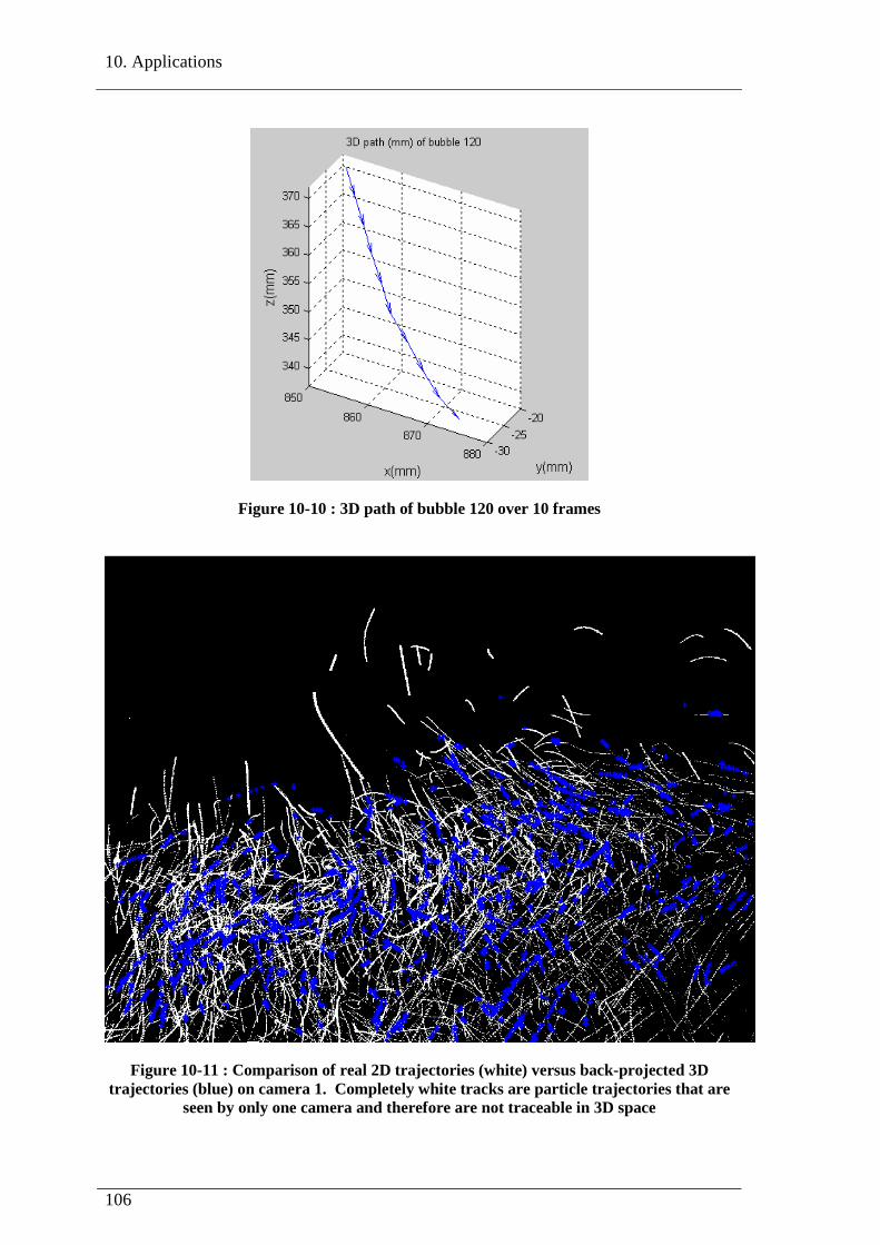
10. Applications
106
Figure 10-10 : 3D path of bubble 120 over 10 frames
Figure 10-11 : Comparison of real 2D trajectories (white) versus back-projected 3D trajectories (blue) on camera 1. Completely white tracks are particle trajectories that are
seen by only one camera and therefore are not traceable in 3D space

10. Applications
107
10.3 Velocity distribution over a heat source
An electric heater was placed against one wall of the Room Ventilation Simulator. Helium filled bubbles were emitted from two pipes situated on either side of the radiator. The bubble generation was not stopped during the recording to prevent their rarefaction due to the upward convection flow. In order to avoid any impact of the bubble initial velocity (5.33m/s) on the measured flow, the pipes nozzles were facing downwards. Therefore, the tracers were recorded from the radiator height (90cm) after rebounding on the floor.
One camera was placed parallel to the wall and looking downward at the field. The other two were facing the wall at a symmetrical angle of 45°. To avoid illuminating the background (wall), the spotlights were also placed parallel to the wall on both sides of the heater (see
Figure 10-13 : Calibration target reference frame from camera 3 viewpoint). The targeted measurement field was the area above the heater. The calibration target was placed over the heater as shown in Figure 10-13.
The heating power was set at 600W. Eight T type thermocouples were set to record the temperature of the wall and of the air above the heater (10cm from the wall). The temperature distribution was 28.5°C on the wall, 29.8°C above the heater and 29.2°C at the center of the room six feet from the wall and three feet from the floor.
Due to the chimney effect, many particles were driven off the measurement field. Therefore, the tracking was performed as in low density cases. Index ξ equalled 3.3, 3.9, and 4.8 respectively for cameras 1, 2 and 3. Results of 3D PTV over the heater are shown in Figure 10-14, 10-13 and 10-14. Tracking indexes were E2Dtrack = 95/138 for camera 1, 73/90 for camera 2 and 61/65 for camera 3 with γ2D = 1. We found E3Dtrack ≈ 106/140 with γ3D = 0.95.
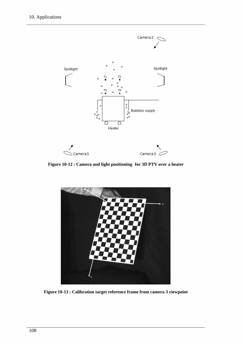
10. Applications
108
Figure 10-12 : Camera and light positioning for 3D PTV over a heater
Figure 10-13 : Calibration target reference frame from camera 3 viewpoint

10. Applications
109
Figure 10-14 : 3D path of bubbles above the heater throughout 30 frames
Figure 10-15 : Comparison of real 2D trajectories (white) versus back-projected 3D trajectories (blue) on camera 1. Completely white tracks are particle trajectories that are seen by only one camera and therefore are not traceable in 3D space. The measured area
is approximately 1.5m x 0.9m x 1.5m high

10. Applications
110
(a)
(b)
(c)
Figure 10-16 : Bubbles 3D paths projected on image plane of cameras 1, 2 and 3 (respectively figures 10-14a, 10-14b and 10-14c). The measured area is approximately
1.5mx0.9mx1.5m high

10. Applications
111
High velocity particles could be captured as dots by the cameras but their inter frame displacement did not allow reliable tracking. Therefore, we resorted to particle streak velocimetry. Particle streaks were obtained by increasing the exposure time of the recording cameras. Low speed particles were still seen as dots but image processing allowed removing them from the images. Streaks pixel length and orientation were calculated as the length and orientation of the major axis of the ellipse that has the same normalized second central moments as the streak’s region. Spatial matching was done as in Section 8 with each streak considered as a trajectory. Streak direction was determined empirically. A precise method to derive the flow direction from the exposure time of each camera has been addressed by Scholzen and Moser (1996). The velocity was given by dividing the length of each streak by the time of exposure. The results of particle streak velocimetry are shown in Figure 10-15.
From the 3D data, the maximum bubbles velocity was found to equal 0.851m/s above the heater while the minimum equaled 0.1m/s.
(a) (b)
(c)
Figure 10-17 : 3D particle streaks from high-velocity particles

10. Applications
112
10.4 Velocity distribution in an experimental aircraft cabin
The experimental aircraft cabin used is a full-scale, fully equipped five row section of a Boeing 767-300 with mannequins to simulate passengers (see Figure 10-16). The cabin is 4mx3mx2m high.
Helium filled bubbles were introduced from two pipes situated at the sides of the ceiling middle section. The aircraft ventilation system was on. The air came from two ventilation inlets located on two sides of the ceiling mid-section (see Figure 10-16). Three cameras were placed outside of the cabin in a triangular pattern. They were directed convergently, with a large triangular base. The calibration target was composed of a checkerboard with 6cm-large black and white squares as shown in Figure 10-17.
Light was provided by eight out of thirty-six 120W light bulbs. Two extra 500W spots were facing the cabin from the external side of the glass wall. Index ξ equalled 2.1, 2.3, and 2.3 respectively for cameras 1, 2 and 3. Due to these very hard tracking conditions, we used the modified fast normalized cross-correlation 2D tracking scheme over 10 frames. E2Dtrack averaged 0.4 over the three cameras with γ2D = 1 and a total of 1083 particles were 3D tracked. E3Dtrack averaged 0.63 with index γ3D = 0.7. Instantaneous 2D velocity profiles obtained and shown on Figure 10-21 were similar to those obtained by Wang et al. (2005) on the same setup. Especially, the same vortices due to recirculation of the air over the two aisles could be observed and 3D tracked.
The mean velocity equaled 0.48m/s over the cabin, with a minimum at 0.018m/s which means quasi static air far from the ventilation nozzles. The 3D data enabled the precise identification of areas of minimum displacement of the air.
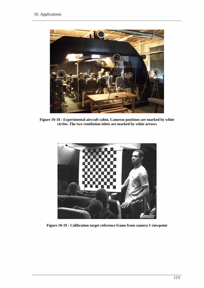
10. Applications
113
Figure 10-18 : Experimental aircraft cabin. Cameras positions are marked by white circles. The two ventilation inlets are marked by white arrows
Figure 10-19 : Calibration target reference frame from camera 1 viewpoint

10. Applications
114
Figure 10-20 : Instantaneous 3D velocity of bubbles in the experimental aircraft cabin using the fast normalized cross-correlation temporal tracking scheme
Figure 10-21 : Instantaneous 2D velocity in the aircraft cabin using the fast normalized cross-correlation temporal tracking scheme. Vortices due to recirculation of the air in the cabin can be seen over the aisles. University of Illinois at Urbana-Champaign, Department of Agricultural and Biological Enginneering, Bioengineering Research Laboratory, USA

10. Applications
115
10.5 3D PTV in a aqueous medium
10.5.1 Context
The turbulent flow of the coolant or neutron moderator liquid past fuel rods usually causes vibrations, and with time, reduces the rigidity of the fuel bundle in Boiled Water Reactors (BWR) and causes wear of the pressure tubes. To increase the safety and efficiency of existing and future nuclear plants, it is important to understand this wear process and minimize the vibrations. In this regard, information about the spatio-temporal velocity distribution around each fuel rod is crucial. This may eventually lead to optimizing the diameter of the pressure tubes, the number of bearing pads and of the spacers between the fuel rods. Numerical models of fuel rod vibration (Chen 1973, Zdravkovich 1973, Chen 1975, Abbasian et al. 2009) are generally regarded as inaccurate and need to be improved and validated by experimental data.
Experimental measurement of rods vibration in test rigs is usually done using pressure measuring transducers. The pressure tabs must feature a wide-band dynamic pressures capability, have a very small pressure sensing area to increase their spatial resolution, and they need to be waterproof in highly pressurized environments (generally on the order of 200KPa). Transducers which meet these requirements are generally of the piezoelectric type, or made of piezoresistive semiconductor material. Savkar and So (1978) used piezoelectric transducers to measure the buffeting forces on a cylinder submitted to cross axial flow. Curling and Papadoussis (1992) used pressure transducers and accelerometers to measure the turbulent wall pressure fluctuations in a square array of 5.72cm-large cylinders in axial flow. Dynamic pressure transducers were also placed along the flow by Meher and Rao (2006) to optimize the number of spacers in a nuclear fuel. Pressure transducers may also serve to separate the noisy vibrations caused by the coolant pumping system from the vibration due to the actual flow (Mulcahy et al. 1980, Wambsganss and Zaleski 1970, Smith and Derksen 1988). To achieve this, they are placed at diametrically opposed locations on the fuel bundle walls.
In spite of their relatively high precision, pressure tabs suffer from two main shortcomings. First, to meet the requirements above mentioned, they generally have to be upgraded, individualized and carefully calibrated for each experimental environment. Second, when mounted on the fuel rod, surface pressure transducers must be highly flushed and aligned with the rod surface in order to avoid disturbances of the flow by eddies at the transducer surface. Such disturbances cannot totally be avoided. Besides, piezoelectric transducers mounted in the rod wall perform poorly on flexible rods because of strain effects from the rod interfering with the pressure effect of the fluid (Mulcahy et al. 1980).
Non-intrusive optical techniques have also been used to measure rod vibration. Among them, laser Doppler velocimetry (LDV) uses two laser beams to create a measuring volume inside the fluid. The velocity of the particles crossing the volume is derived from their observed variation of frequency (Doppler Effect). The measurement is

10. Applications
116
usually conducted through glass windows set on the test rig. LDV measurements in experimental fuel rod bundles include the works of Creer et al. (1979, 7x7 rod array, eight inches squared section, water 85°F, Remax=5.8e4), Neti et al. (1982), Simonin and Barcouda (1988), Yang and Chung (1998), Ikeda and Hoshi 2006 (5x5 rod array, 65mm square section, water 300K, Remax=5.7e4), Chang et al. (2008).
Though LDV provides a very high time resolution (typically over 100 kHz), it suffers from two main limitations: First, it yields only point-wise velocity data. In order to measure a full cross section, the measuring volume has to be moved successively to precisely located positions (Creer et al. 1979) thus generating an error when dealing with unsteady flow. This is a standard limitation of the LDV technique. Second, some parts of the measured section generally remain uncovered due to the opacity of the fuel rods (Chang et al. 2008).
The latter limitation has been partly overcome by the most recent use of particle image velocimetry (PIV) combined with the matched index-of-refraction (MIR) approach in test fuel bundles (Hassan and Dominguez-Ontiveros 2008). In standard PIV, neutrally buoyant seeded particles are captured on images by using either a 6 to10ns-long pulsed laser or a 0.1 to 100ns-long exposure camera in order to freeze the particle motion. The time between two captures is usually very short, around 100ns. The use of lasers allows imaging only objects present in the laser plane, with a very strong light intensity. Particle velocity is generally calculated by direct cross-correlation of the pattern formed by a group of particles between two frames. The MIR approach consists in making the test-rig optically transparent by the use of a flow liquid whose index of refraction matches the index of refraction of the rig walls at the illumination source wavelength. In the meantime, the non-transparent seeded particles remain always visible.
Dominguez-Ontiveros and Hassan (2009) used the MIR approach to carry out PIV measurements in a 5x5 square array of 10.25mm-large plastic rods with spacer grids. Their test section, including the rods, was made of fluorinated ethylene propylene plastic. Each rod was shallow and filled with a water and chlorine solution to increase its rigidity. Water was used as working fluid. Tracers were 6 to 9µm-large polymer particles with a specific density of 1.05. Their motion was recorded by 120 KHz high speed cameras. Valuable velocity statistics were obtained for axial and cross flows on 2D planes ranging from 5mmx4mm to 70mmx60mm. Although accurate, their method suffers from two natural limitations of PIV: firstly, only 2D velocity vectors are yielded. Even stereoscopic PIV only yields field-wise 3D velocity vectors inside thin laser sheets. The particles situated outside of the 0.5 to 5mm-deep laser sheet are not viewed. Secondly, only instantaneous velocity fields are acquired by PIV. Particles trajectories are not recovered.
In the following, we propose a method combining 3D particle tracking velocimetry (3DPTV) and the MIR approach. Unlike PIV, 3DPTV yields particle 3D trajectories in full 3D volumes. The simultaneous use of at least three calibrated and time–

10. Applications
117
synchronous cameras gives access to the 3D positioning of each particle through 3D triangulation. Depending on the flow velocity, the camera frame rate (typically from 30 to 120fps) is adjusted to catch the displacement of each particle, thus yielding its 3D trajectory. In our research work, continuous white light is used instead of pulsed lasers in order to increase the measuring volume.
10.5.2 Experimental hardware
A feasibility study was conducted on a simplified test section whose set-up closely follows the MIR approach. The test-rig consisted of a 200x100x100mm high Plexiglas container. A vertical Plexiglas bar with a diameter of 17mm crossed the tank from top to bottom. The container was filled with an aqueous calcium chloride solution. The refraction index of the solution was very close to the one of the Plexiglas so that the bar would progressively disappear as the container was filled. To create fluid motion, a magnetic shaker was placed inside the tank. The test-rig is shown in Figure 10.22.
Figure 10-22 : The figure shows one side of the 200mmx100mmx100 mm high Plexiglas containers. The index of the aqueous solution makes the included Plexiglas cylinder
invisible. Its actual position is showed by white arrows
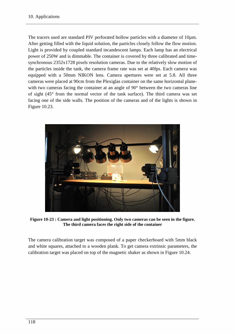
10. Applications
118
The tracers used are standard PIV perforated hollow particles with a diameter of 10µm. After getting filled with the liquid solution, the particles closely follow the flow motion. Light is provided by coupled standard incandescent lamps. Each lamp has an electrical power of 250W and is dimmable. The container is covered by three calibrated and time-synchronous 2352x1728 pixels resolution cameras. Due to the relatively slow motion of the particles inside the tank, the camera frame rate was set at 40fps. Each camera was equipped with a 50mm NIKON lens. Camera apertures were set at 5.8. All three cameras were placed at 90cm from the Plexiglas container on the same horizontal plane- with two cameras facing the container at an angle of 90° between the two cameras line of sight (45° from the normal vector of the tank surface). The third camera was set facing one of the side walls. The position of the cameras and of the lights is shown in Figure 10.23.
Figure 10-23 : Camera and light positioning. Only two cameras can be seen in the figure. The third camera faces the right side of the container
The camera calibration target was composed of a paper checkerboard with 5mm black and white squares, attached to a wooden plank. To get camera extrinsic parameters, the calibration target was placed on top of the magnetic shaker as shown in Figure 10.24.

10. Applications
119
Figure 10-24 : Calibration target used for 3DPTV in an aqueous calcium chloride solution. Due to the smallness of the targeted area, the checkerboard is composed of 5mm squares.
The target is placed onto the magnetic plate where the cylinder will later be installed
10.5.3 Results and discussion
The data from the particle detection step show that a perfect optical transparency of the rig wall is crucial to avoid false centroid detection. After image processing, the particle center calculation algorithm detected 842, 300 and 741 centroids for cameras 1, 2 and 3. However, a close examination and comparison of centroid images to raw particle images showed that around 30% of the calculated centroids were actually tiny imperfections in the rig wall (see Figure 10.25). Those imperfections were barely visible with the human eye but were revealed and enhanced by the image processing step. Some of the fake centroids were removed by thresholding or blackening some areas of the images. The actual number of particle centers was around 590, 210 and 593 for cameras 1, 2 and 3.

10. Applications
120
Figure 10-25 : Sample particle image after image processing (the image is binarized and inverted for clarity sake). Particles are introduced from the top right angle of the image. An imperfection on the container wall can be seen in the center of the picture in the form
of a black elliptical shape
Figure 10-26 : Result of the 2D tracking. Trajectories are colored from blue (trajectory start) to red (trajectory end). Imperfections in the container wall can still be seen in the
lower half of the image

10. Applications
121
Index ξ (ratio of mean particle spacing to mean particle displacement between two consecutive frames) was 3.7, 9.8 and 4.6 for cameras 1, 2 and 3. Such values of ξ mean relatively easy 2D tracking conditions. The temporal tracking over a 30-frame displacement yielded E2Dtrack = 365/590 for camera 1, 161/200 for camera 2 and 188/518 for camera 3 with γ2D = 1. Figure 10.26 shows a sample image from the 2D tracking step.
The spatial matching and triangulation steps allowed recovering 140 correct 3D trajectories. The overall 3D tracking performance was E3Dtrack = 0.25% with γ3D > 0.95. The latter values mean that only one fourth of the particles initially present in the container were correctly 3D tracked. This is due to a poor overlapping of the cameras fields of vision. Basically, each camera individually saw many particles, but those particles were not the same one observed by the other two cameras. Therefore, the stereo matching step of the algorithm discarded many 2D trajectories. This observation makes crucial the use of at least four cameras in the full-scale test-rig to ensure that every part of the measuring volume is being seen by at least two cameras. From the 3D data, the maximum velocity in the tank was found to be 1.9mm/s with a mean value at 0.3mm/s.
This research work showed that 3DPTV combined with the MIR approach is a promising way of getting Lagrangian statistics of the coolant flow around the fuel rods. In order to increase the measuring volume, continuous white light can be used instead of lasers, provided a high transparency of the test-rig walls and rods, and a very good matching with the coolant index of refraction have been secured. Then, seeded particles can easily be detected after background subtraction. Many 3D particle trajectories can be recovered after 3D reconstruction provided all parts of the measuring volume are covered by at least two cameras. For a 100mmx100mmx200mm targeted volume, a four-camera arrangement is optimal. The 3DPTV procedure described here might be used in existing full scale and optically transparent fuel bundle test-rigs.
Acknowledgement: This research work was partly supported by a grant from the AREVA Group.

11. Conclusion
122
11 Conclusion
11.1 Overview of the achievements
First, we investigated several experimental velocimetry procedures, namely: Pitot static tubes, hot wire and hot film anemometry, pulsed wire and ion anemometry, sonic anemometry, laser Doppler anemometry, laser induced fluorescence velocimetry, laser 2-focus velocimetry, magnetic resonance velocimetry, particle image velocimetry, particle streak velocimetry and particle tracking velocimetry. It was determined that 3D PTV is among the best tools when measuring large scale indoor air motion. This is due to its capability to measure both the 3D instantaneous distribution and the 3D trajectories of airflow regions with satisfactory spatial and temporal resolution and with virtually no speed limit (except the limit on the speed of modern cameras).
Among the tracers used in the air, helium filled soap bubbles are well suited for measurements in volumes over 1m3 and are used by scientists worldwide for this type of application. They provide a spatial resolution of 3mm. It was shown that along with neutrally buoyant bubbles, some lighter than air particles are produced by commercially available generators. By ensuring the elimination of the particles lighter than the air in environments with weak gradients of pressure as is the case for free displacements in rooms, even not perfectly neutral particles do follow the flow. A set-up to remove lighter-than-air particles was proposed.
Our testing of various types of light sources demonstrated that continuous white light is both a valid and flexible solution for 3D PTV in large volumes.
The multi-camera calibration technique used is halfway between photogrammetric calibration and self-calibration. Instead of a full 3D calibration object, a 2D planar checkerboard is moved to about 10 different locations. The method for the initial estimation of planar homographies and the final maximum likelihood estimation is the one proposed by Zhang (1999). The closed-form estimation of camera intrinsic parameters explicitly uses the orthogonality of vanishing points as presented in Beardsley and Murray (1992). Tangential distortion coefficients are also estimated following the camera model proposed by Heikkilä and Silvén (1997).
Our procedure to remove blobs suppresses untraceable particle images when 3D PTV is conducted with a small distance of the cameras from the measuring volume. Such a situation is
likely to occur in many standard rooms. We demonstrated that due to multiple local maxima for a single particle image, weight averaged methods are best suited to calculate the centers of helium filled bubbles.
Two temporal tracking schemes are used. The first one is based on fast normalized cross-correlation with Lagrangian extrapolation in image space to solve ambiguities. The second uses polynomial regression to find an estimated position and applies a quality criterion based on a minimization of changes in particle acceleration; it also

11. Conclusion
123
includes a cross gap strategy which permits finding a trajectory even if there is a one frame gap in the particle’s temporal detection. By recalculating particle centroids at each time step, the algorithm detects and creates a new trajectory for any new particle entering the field of vision. This scheme allows backward temporal tracking. While the first scheme gives better results for short trajectories, the second scheme has proven more robust against noise and yields longer trajectories than most traditional algorithms (Li 2008). The computational cost of the two algorithms in terms of space and time is higher than the cost incurred by most traditional algorithms.
The spatial matching of the 2D trajectories obtained can be addressed by the well known epipolar constraint (Maas 1992) or by directly sorting the 3D coordinates of particles calculated by two cameras at a time. But unlike most traditional algorithm, our algorithm checks spatial matching at several points throughout the entire length of the trajectory instead of doing it once before the tracking in object space (Willneff 2002, Kasagi and Nishino 1991). This novel scheme yields more reliable correspondences. To increase the number and length of trajectories, the correspondence problem is resolved by only two cameras whenever particles are not seen by all three cameras at the same time. Calculation of bubbles 3D coordinates is done by resolving the over-determinated system of equations generated by the multiple viewpoints using a least squares method.
We showed successful applications of the algorithm on four experimental indoor set-ups. The experiments included Lagrangian tracking inside a 3.1mx3.1mx2.5m high light-gray walled test-room with low particle density, in a 5.5mx3.7mx2.4m high black walled test-room with high particle density, over a heat source, and in a 4mx3mx2m high Boeing 767-300 cabin with mannequins to simulate passengers. The algorithm was also tested in an aqueous medium with continuous light and 10µm-large hollow particles. For each experimental case, light and camera positioning are fully described. This positioning is actually the longest part of the 3D PTV set-up process, especially in large volumes because all particles must be homogeneously lit with good background contrast.
Estimation of accuracy is made by comparing 3D paths to raw experimental particle trajectories. For tracked particles, the 2D distance between real trajectories (obtained by image addition) and calculated trajectories (obtained after back-projection of 3D data on 2D camera image planes) was less than the particles pixel diameter which is 2 to 6 pixels depending on the experimental case.
Up to 1083 bubbles were tracked in volumes up to 3mx3mx1.2m high. However, from simulation data, we found that the proposed algorithm can track in 2D more than 1800 particles in 2000x2000 pixels images and around 1400 particles after 3D matching. For tracked trajectories, the ratio of number of tracked positions which were identical to real 2D particle positions divided by the total number of tracked positions γ was always over 0.97 after temporal tracking and above 0.7 after 3D triangulation. The overall ratio of

11. Conclusion
124
number of correctly tracked 3D trajectories divided by the total number of trajectories E3Dtrack would vary between 0.25 and 0.88, depending on the particle density. It shows that even in difficult tracking circumstances where the ratio of mean particle spacing (in a nearest neighbor sense) to mean displacement of particles between two consecutive frames ξ was smaller than 3, the few particles tracked in 2D and 3D spaces are correctly tracked.
Finally, we proposed a particle images simulation toolbox and a complete 3D PTV toolbox for Matlab. The 3D PTV toolbox uses particle images from three calibrated viewpoints and a few experimental parameters as inputs. It yields 3D trajectories, successive 3D velocities and accelerations as well as image plane trajectory of each particle. The toolbox processing closely follows the steps and methods mentioned above. Several post-processing options are included in the toolbox such as displaying of 3D trajectories and the representation of instantaneous 2D velocity fields. An Error Analysis tool permits checking of the overall 3D tracking process accuracy.
The complete algorithm for 3D particle tracking in rooms is the result of a joint research conducted in the Thermal Sciences Research center of Lyon (CETHIL), France, and in the Bio Environmental Engineering Laboratory of the University of Illinois at Urbana-Champaign, USA. Our work is a step forward in exploring the requirements and capabilities of 3D PTV applied to indoor air. Along with the novel temporal tracking and spatial matching procedures searched, we applied the method on a wide range of indoor situations. Complete description of light and camera positioning are given for each experimental case. Such guidelines are rarely found in literature on 3D PTV for indoor applications.
11.2 Limitations of the method
The first and main limitation of our 3D PTV procedure comes from particle density. As shown in the experimental results section, a too high density of tracers leads to problems both in particle identification due to the overlapping of bubble images and in temporal tracking. This is a standard limitation of 3D PTV. The second limitation is due to the tracers used. The diameter of the bubbles does not allow the study of turbulence from Kolmogorov to millimetric scales. Besides, the current lifetime of the bubbles does not permit a Lagrangian tracking process over two minutes. Some measures have been searched to expand the bubbles’ lifetime (Machacek 2002) but with insufficient assessment of the resultant buoyancy. The last limitation comes from current camera lenses which have a finite object field depth. Due to that limitation, the extension of the measurement to very large volumes is difficult when using a single multi-vision system of three or four cameras.

11. Conclusion
125
11.3 Recommendations
- Bubble generation: Bubble production should be stopped a few seconds before starting the recording in order to keep the flow undisturbed by the air velocity at the bubble generator pipe nozzle. A cold soap liquid dramatically increases the number of bubbles produced. Consequently, bubble film liquids must always be kept in a nearby refrigerator.
- Choice of devices: Four cameras is an optimal number to remove ambiguities when doing 3D PTV. Powerful continuous white light is adapted to tracking in large volumes. To prevent heating, light sources should be situated outside of the room behind a glass partition when possible. Otherwise, they must be turned on only for the few seconds of recording.
- Particle detection: Particles should be lighted up by indirect reflection on walls when doing 3D PTV in a non-white room. In a black room, light can be focused directly onto the particles. It is generally better to provide the particle center detection algorithms with non-homogeneous intensity profile particles image. So, one should avoid calculating particle centers from binarised, bridged or filled-up particle images.
- Temporal tracking: The modified cross-correlation scheme gives better results in cases of short trajectories (< 10 frames). In other circumstances, the polynomial regression scheme is more appropriate.
- 3D reconstruction: Widely separated and convergent viewpoints help improve the accuracy of spatial matching and the accuracy of the in-depth coordinate.
11.4 Perspectives
- Further improvements in the algorithm: From temporal tracking data, the creation of artificial trajectories by grid extrapolation should be possible in appropriately dense images. By projecting those artificial particles in 3D space, we should have access to a more complete image of the velocity distribution in rooms. The algorithm should be rethought and rewritten to include a fourth camera. The measurement area can be increased by juxtaposing several multi-camera PTV systems so that every part of the volume is covered by at least two cameras.
- Building applications: Our 3D PTV system already provides CETHIL with a new tool of Lagrangian motion measurement. There are plenty of short term applications of the current algorithm for energy efficient buildings research. For example, the impact of free heat loads could be assessed by finding the velocity distribution over a solar beam. It is worth mentioning that the 3D PTV algorithm can be used in media other than air, provided suitable light source and tracers are used. Our application of 3D

11. Conclusion
126
PTV in a Plexiglas tank containing an aqueous calcium chloride solution confirms this assertion.
- Particle image thermometry: Combining particles Lagrangian velocity with particles Lagrangian temperature would be a great achievement. When trying to get fluid temperature from particle images, three approaches are possible. First, one could try to link changes in temperature to changes in particle density and thus in particle radius. This first approach is not valid because of the following rationale: Let V0 be the initial volume of a particle and β is the coefficient of volumetric thermal expansion of helium at constant usual pressure. We can write:
TV
V ∆=∆ β0
(11-1)
Then, if V1 is the new volume of the particle, we obtain:
( )101 +∆= TVV β (11-2)
If we assume that the coefficient of volumetric thermal expansion of helium at 20°C and usual pressure is close to the one of the air, i.e., 3.43x10⁻³K-1, we conclude that in most cases:
01 VV ≈ (11-3)
Actually, it would require a temperature difference on the order of 103K to make a change of particle size apparent. Besides, this change would have to be compensated with respect to the displacement of the particle towards or away from the camera.
A second approach is to directly link an upward acceleration of the particle to a local change in temperature. But this would require preliminary calibration and a completely sealed experimental room to prevent air motion from an external source, which is almost impossible to obtain in practice.
The last and most realistic approach is to create heat-sensitive fluorescent bubble shells that visually and reversibly change colors at predetermined temperatures. In this regard, the use of thermochromic liquid crystals (Koch 1993, Kowalewski 2009) or of polythiophene films (Lucht et al. 2002) could be of some interest. However, this approach would require camera sensors that are highly sensitive to color change. Much research is still ahead!

11. Conclusion
127

References
128
References
Abbasian F., Yu S.D. and Cao J. (2009) Experimental and numerical investigations of three-dimensional turbulent flow of water surrounding a CANDU simulation fuel bundle structure inside a channel, Nuclear Engineering and Design, In Press
Adrian R.J. (1991) Particle-imaging techniques for experimental fluid mechanics, Annual Review of Fluid Mechanics 23, pp. 261–304
Adrian R.J. (2005) Twenty years of particle image velocimetry, Experiments in Fluids 39, pp. 159-169
Adamczyk A.A, Rimai L. (1988) Reconstruction of a 3-dimensional flow field from orthogonal views of seed track video images, Experiments in Fluids 6, pp. 380-386
Agui, Jimenez J.C. (1986) On the performance of particle tracking. Journal of Fluid Mechanics 185, pp. 447-468
Anonymous (1988) SAI Bubble Generator: Description and Operating Instructions. Sage Action, Inc., New-York; Available on website http://www.sageaction.com/ (consulted on November 20, 2006)
Barber R.W., Emerson D.R. (2001) Numerical Simulation of Low Reynolds Number Slip Flow Past a Confined Microsphere Centre for Microfluidics, Department of Computational Science and Engineering, CLRC Daresbury Laboratory, Technical Report DL-TR-01-001
Basset A.B. (1888) Treatise on hydrodynamics, London: Deighton Bell and Co, vol. 2, chap.22, pp. 285-297
Beardsley P., Murray D. (1992) Camera calibration using vanishing points, Department of Engineering Science, University of Oxford, Oxford OX1 3PJ, UK
Biwole P.H., Krauss G., Favier E. Rusaouen G., Roux J.-J. (2008) Non-stereoscopic 3D particle tracking velocimetry for full scale rooms, Proceedings of Advanced building ventilation and environmental technology for addressing climate change issues, Kyoto, Japan, October 2008
Bougnoux S. (1998) From projective to Euclidean space under practical situation, a criticism of self calibration, Proc. 6th European conference on computer vision, pp. 790-796, January 1998
Bouguet Jean-Yves (2002), Camera Calibration Toolbox for Matlab, Available on website http://www.vision.caltech.edu/bouguetj/calib_doc/ (consulted on October 8, 2007)
References
129
Boussinesq J. (1903) Théorie analytique de la chaleur, Ecole Polytechnique, Paris, vol. 2, pp. 224
Carosone F., Cenedese A., Querzoli G. (1995) Recognition of partially overlapped particle images using the Kohonen neural network, Experiments in Fluids 19, pp. 225–232
Caprile B., Torre V. (1990) using vanishing points for camera calibration, The International Journal of Computer Vision 4 (2), pp. 127-140
Chang S.K., Moon S.K., Baek W.P., Choi Y.D. (2008) Phenomenological investigations on the turbulent flow structures in a rod bundle array with mixing devices, Nuclear Engineering and Design 238, pp. 600–609
Chen S.S. (1975) Vibration of nuclear fuel bundles, Nuclear Engineering and Design 35, pp. 399-422
Chen Y.N. (1973) Fluctuating lift forces of the Karman vortex streets on single circular cylinders and in tube bundles, Part 2 - criterion for the fluid elastic orbital vibration of tube arrays, ASME Paper No. 73-Det-146
Chetverikov D., Verestoy J. (1998) Tracking feature points: A new algorithm, Computer and Automation Research Institute Budapest, Kende u.13-17, H-1111 Hungary Corrsin S., Lumley J. (1956) On the equation of motion for a particle in turbulent fluid, Applied Science Research A 6, pp. 114-116
Creer J.M., Bates J.M., Sutey A.M., Rowe D.S. (1979) Turbulent flow in a model nuclear fuel rod bundle containing partial flow blockages, Nuclear Engineering and Design 52, pp. 15-33
Curling L.R., Paidoussis M.P. (1992) Measurements and characterization of wall-pressure fluctuations on cylinders in a bundle in turbulent axial flow; part 1: spectral characteristics, Journal of Sound and Vibration 157(3), pp. 405-433
Dantec Dynamics. Available on website <http://www.dantecdynamics.com> (consulted on November 6, 2008)
David L., Gicquel P. (2006) Évolution de la technique PIV à travers quelques conférences internationales de 2000 à aujourd'hui, Congrès Francophone de Techniques Laser, Toulouse, september 2006.
Dimotakis P.E., Debussy F.D., Koochesfahani M.M. (1981) Particle streak velocity field in two-dimensional mixing layer, Physics of Fluids 24, p. 995

References
130
Dominguez-Ontiveros E.E. and Hassan Y.A. (2008) Non-intrusive experimental investigation of flow behaviour inside a 5×5 rod bundle with spacer grids using PIV and MIR, Nuclear Engineering and Design 239, pp. 888–898
Dracos Th. (1996) Particle tracking in three-dimensional space, In: Three-dimensional velocity and vorticity measuring and image analysis techniques, Dracos Th (ed) Kluwer, Dordrecht
Dursapt M. (2009) Aide mémoire, Métrologie dimensionnelle, Dunod, Paris, 2009, p. 49
Elkins C.J., Alley M.T. (2007) Magnetic resonance velocimetry: applications of magnetic resonance imaging in the measurement of fluid motion, Experiments in Fluids 43, pp. 823-858
Elsinga G., Van Oudheusden B., Scarano F. (2005) Assessment of Tomo-PIV for three dimensional flows, 6th International Symposium on Particle Image Velocimetry, Pasadena, USA
Einstein A. (1906), Eine neue Bestimmung der Moleküdimensionen, Annalen der Physik 19, pp. 289–306
Einstein A. (1911) Berichtigung zu meiner Arbeit: Eine neue Bestimmung der Moleküdimensionen, Annalen der Physik 34, pp. 591–592
Faugeras O. (1993) Three-dimensionl computer vision: a geometric viewpoint, London: MIT press, 1993, 663 p.
Favier E., Dursapt M. (2005) Mesures de formes bidimensionnelles. Etude d’un moyen de mesure par vision numérique, In : Lavoisier, Métrologie, science transversale : De la mécanique à la physico-chimie (Instrumentation Mesure Métrologie RS série I2M - Vol. 5 N° 3-4/2005), pp. 59-74
Föster W., Karpinsky G., Krain H., Röhle I, Schodl R. (2000) 3-component-Doppler-laser focus velocimetry applied to transonic centrifugal compressor, In Adrian, R.J., Durao D.F.G., Heitor, M.V. Laser techniques for fluid Mechanics, Selected Papers from the 10th International Symposium Lisbon, Portugal July 10-13, 2000. Germany: Institute of Propulsion Technology, 12 p.
Gruen A., Baltsavias E. (1988) Geometrically constrained multi-photo matching, Photogrammetric Engineering 54, pp. 633-641
Guezennec Y.G., Brodkey R.S., Trigui N., Kent J.C. (1994) Algorithms for fully automated three-dimensional particle tracking velocimetry, Experiments in Fluids 17, pp. 209–219

References
131
Hartley R. (1994), Self calibration from multiple views with a rotating camera, Proceedings of 3rd European Conference on Computer Vision, Stockholm, Sweden May 1994, pp. 471-478
Hartley R., Zisserman A. (2000) Multiple View Geometry in Computer Vision, Cambridge: Cambridge University Press, pp 297-298, ISBN: 0521623049
Hassan Y.A. and Dominguez-Ontiveros E.E. (2008) Flow visualization in a pebble bed reactor experiment using PIV and refractive index matching techniques, Nuclear Engineering and Design 238, pp. 3080–3085
Heikkilä J., Silvén O. (1997) A Four step camera calibration procedure with implicit image correction, Conference on Computer Vision and Pattern Recognition (CVPR’97), San Juan, Puerto Rico
Hough P. (1962) Method and means for recognizing complex patterns, U.S. Patent 3069654
Husson J. (1979) Le contrôle statistique de la qualité, Paris: PYC Edition-Desforges, 1979, p. 24
Ikeda K., Hoshi M. (2006) Development of rod-embedded fiber LDV to measure velocity in fuel rod bundles, Journal of Nuclear Science and Technology 43, pp. 150–158
Jeffrey D.J. (1977) The physical significance of non-convergent integrals in expressions for effective transport properties. In: Continuum Models of Discrete Systems, Proceedings of the Second International Symposium, Provan, J.W. (Ed.), University of Waterloo Press, Waterloo, Canada, pp. 653–674
Kasagi N., Nishino K. (1991) Probing turbulence with three-dimensional particle tracking velocimetry, Experimental Thermal and Fluid Science 4, pp. 601-610
Kerho M.F., Bragg M.B. (1994) Neutrally buoyant bubbles used as flow tracers in air, Experiments in Fluids 6, pp. 393-400
Kessler M., Leith D. (1991) Flow measurement and efficiency modeling of cyclones for particle collection, Aerosol Science and Technology 15, pp. 8-18
Koch S. (1993) Non-intrusive measurement of temperature and velocity in free convection (Berührungslose Messung von Temperatur und Geschwindigkeit in freier Konvektion). Ph.D.Thesis in Mitteilungen aus dem MPI 108, Göttingen
Kowalewski T.A. (2009) Particle image velocimetry and thermometry using thermochromic liquid crystals. IPPT PAN, Polish Academy of Sciences Center of Mechanics and Information Technology Swietokrzyska 21, PL - 00049 Warszawa

References
132
Kuznik F. (2002) Vélocimétrie par images de particules ; Application aux grandes cavités fermées. Rapport de stage de DEA. Villeurbanne : Centre de Thermique de Lyon, Institut National des Sciences Appliquées de Lyon, 2002
Kuznik F. (2005) Etude expérimentale des jets axisymétriques anisothermes horizontaux se développant près d’une paroi. Application à la modélisation numérique des cavités ventilées. PhD Thesis, Villeurbanne : Institut National des Sciences Appliquées de Lyon, 2005, 190 p.
Lauterbur P.C. (1973) Image formation by induced local interactions: examples employing nuclear magnetic-resonance, Nature 242 (5394), pp. 190–191
Lercef A., Renou B., Allano D., Boukhalfa A., Trinite M. (1999) Stereoscopic PIV: validation and application to an isotropic turbulent flow, Experiments in Fluids 26, pp. 107-115
Lewis J.P. (1995) Fast Template Matching, Vision Interface, pp. 120-123
Li D., Zhang Y., Sun Y., Yan W. (2008) A multi-frame particle tracking algorithm robust against input noise, Measurement Science and Technology 19, 105401 (11pp)
Liebowitz D., Zisserman A. (1998) Metric rectification for perspective images of planes. Proceedings of IEEE conference on computer vision and pattern recognition, Santa Barbara, California, June 1998, pp. 482-488
Lucht B.L., Euler W.B., Gregory O.J. (2002) Investigation of the thermochromic properties of polythiophenes dispersed in host polymers. Departments of Chemistry and Chemical Engineering, University of Rhode Island Kingston, RI 02881
Luong Q.T., Faugeras O. (1997) Self-calibration of a moving camera from point corespondances and fundamental matrices, The International Journal of Computer Vision 22 (3), pp. 261-289
Maas H.G. (1992) Complexity analysis for the establishment of image correspondences of dense spatial target fields, International Advances of Photogrammetry and Remote Sensing, XXIX (B5), pp. 102-107
Maas H.G., Gruen A., Papantonious D. (1993) Particle tracking velocimetry in three-dimensional flows, Experiments in Fluids 15, pp. 133-146
Machacek M. (2002) A Quantitative Visualization Tool for Large Wind Tunnel Experiments. PhD Thesis, Zurich: Swiss Federal Institute of Technology
Malik N.A., Dracos Th., Papantoniou D.A. (1993) Particle tracking velocimetry in three-dimensional flows—part 2: Particle tracking, Experiments in Fluids 15, pp. 279–294

References
133
Mann J., Ott S., Andersen J.S. (1999) Experimental study of relative, turbulent diffusion. Risø National Laboratory Report Risø-R-1036 (EN)
Maybank S.J., Faugeras O. (1992) A theory of self-calibration of a moving camera, The International Journal of Computer Vision 8(2), pp. 123-152
Maxey M.R., Riley J.J. (1983) Equation of motion of a small rigid sphere in a nonuniform flow, Physics of Fluids 26 (4), pp. 883-889
Meher Kishor K. and Rama Rao A. (2006) Optimization of the number of spacers in a nuclear fuel bundle with respect to flow-induced vibration, Nuclear Engineering and Design 236, pp.2348–2355
Melling A. (1997) Tracer particles and seeding for particle image velocimetry, Measurement Science and Technology 8, pp. 1406-1416
More J. (1977) The Levenberg-Marquardt algorithm, implementation and theory, In Numerical Analysis, Berlin: Springer-Verlag, pp. 105-116 (lecture Notes in Mathematics 630)
Mulcahy T.M., Lawrence W., Wambsganss M.W. (1980). Dynamic surface-pressure instrumentation for rods in parallel flow, Fourth SESA International Congress on Experimental Mechanics Boston, MA, May 25-30
Muller D., Renz U. (1996) Determination of all airflow velocity components by a particle-image-velocimetry system, ROOMVENT 96, pp. 413-419
Nathan A.M., Bennet L., Cytter M. (1969) Ion anemometer, NY Univ. Bronx Geophysical Sc. Lab. Report number 0444168, 70 p.
Neti S., Eichhorn R., Hahn O.J. (1982) Laser Doppler measurements of flow in a rod bundle, Nuclear Engineering and Design 74, 105–116
Nobach H.,Honkanen M. (2005) Two-dimensional Gaussian regression for sub-pixel displacement estimation in particle image velocimetry or particle position estimation in particle tracking velocimetry, Experiments in Fluids 38 (4), pp. 511-515
Okamoto K., Nishino S., Saga T. and Kobayashi T. (2000) Standard images for particle-image velocimetry Measurement Science and Technology 11, pp. 685–691
Okuno Y., Fukuda T., Miwata Y., and Kobayashi T. (1993) Development of three-dimensional air flow measuring method using soap bubbles. Japanese Society of Automotive Engineers (JSAE) Review 14 (4), pp. 50-55
Oseen C. W. (1927) Hydrodynamik, Leipzig: Akad. Verlagsgesellschaft, 132 p.
Otsu N. (1979) A threshold selection method from gray-level histogram, IEEE Transactions on Systems, Man, and Cybernetics 9, 1, pp. 62-66

References
134
Ouellette N.T., Xu H., Bodenschatz E. (2006) A quantitative study of three-dimensional Lagrangian particle tracking algorithms, Experiments in Fluids 40, pp. 301–313
Prasad A.K. (2000) Stereoscopic particle image velocimetry, Experiments in Fluids 29, pp. 103-116
Resagk C., Lobutova E., Rank R., Müller D., Putze T., Maas H.G. (2006) Tracking of large-scale flow structures in air applying a novel 3D particle tracking velocimetry technique, Proceedings of 13th International Symposium on Application of Laser Techniques to Fluid Mechanics, June 26-29, Lisbon
Sang Joon L., Seok K. (2005) Simultaneous measurement of size and velocity of microbubbles in opaque tube using X-ray particle tracking velocimetry technique, Experiments in Fluids 39 (3), pp. 492-497
Savkar S.D. and So R.M.C. (1978) Buffeting in single cylinders, Proceedings of the Keswick International Conference on vibration in Nuclear Plant,UK, pp. 189-204
Schlichting H. (1968) Boundary-Layer Theory, 3rd English Ed., New-York: McGraw-Hill, 748 p.
Schnars U., Juptner W. (1994) Direct recording of holograms by a CCD target and numerical reconstruction, Applied Optics 33 (2), p. 179
Scholzen F., Moser A. (1996) Three-dimensional particle streak velocimetry for room air flows with automatic stereo-photogrammetric image processing, ROOMVENT 96, Yokohama, Japan, pp. 555-562
Semple J.G., Kneebone G.T. (1952) Algebraic projective geometry, Oxford: Oxford University Press, 1952
Simonin O., Barcouda M. (1988) Measurements and prediction of turbulent flow entering a staggered tube bundle, Proceedings of the 4th international symposium on applications of laser anemometry to fluid mechanics, Lisbon, Portugal, July 1988
Smith B.A. and Derksen D. (1998) Measurement of steady and unsteady hydrodynamic loads on a nuclear fuel bundle, Journal of Fluids and Structures 12, pp. 475-489
Stein G. (1995) Accurate internal camera calibration using rotation, with analysis of sources of errors. Proceedings of the 5th International Conference on Computer Vision, Cambridge, Massachusetts, June 1995, pp. 230-236
Stevenson W.H., Dos Santos R., Mettler S.C. (1975) A laser velocimeter utilizing laser-induced fluorescence, Applied Physics Letters 27 (7), p. 375
Stokes G.G. (1851) On the effect of the internal friction of fluids on the motion of pendulums, Transactions of Cambridge Philosophical Society 9, pp. 8-106

References
135
Svoboda T., Martinec D., and Pajdla T. (2005) A convenient multi-camera self-calibration for virtual environments, PRESENCE: Teleoperators and Virtual Environments, pp 407-422, 14 (4)
Sun Y., Zhang Y. (2003) Development of a stereoscopic particle image velocimetry system for full-scale room airflow studies, Part II: experimental setup. Transaction of the American society of Heating, Refrigerating and Air-Conditioning Engineers (ASHRAE) 09 (2), pp. 540-548
Suzuki Y., Kasagi N. (1999) Turbulent air-flow measurement with the aid of 3-D particle tracking velocimetry in a curved square bend, Flow, Turbulence and Combustion 63, pp. 415-442
Tchen C.M. (1947) Mean value and correlation problems connected with the motion of small particles suspended in a turbulent fluid. Ph.D. Thesis, The Hague: University of Delft, Martinus Nijhoff
Teh Ch., Chin R. (1988) On image analysis by the method of moments, IEEE Pattern Analysis and Machine Intelligence 10 (6), pp. 496-513
Veenman C.J., Reinders M.J., Backer E. (2003) Establishing motion correspondence using extended temporal scope, Artificial Intelligence 145, pp. 227–243
Wambsganss M.W. and Zaleski P.L. (1970) Measurement, interpretation and characterization of near field flow noise, Proceedings of the Conference on Flow Induced Vibrations in Reactor Components, Argonne National Laboratory Report ANL-7685, pp. 112-137
Wasiolek P.T., Whicker J., Gong H., Rodgers J.C. (1999) Room airflow studies using sonic anemometry, Indoor Air 9, pp. 125-133
Willneff J., Gruen, A. (2002) A new spatio-temporal matching algorithm for 3D-ParticleTracking Velocimetry, Proceeding of The 9th International Symposium on Transport Phenomena and Dynamics of Rotating Machinery, Feb 10-14, Honolulu, Hawaii, USA
Yang S.K., Chung M.K. (1998) Turbulent flow through spacer grids in rod bundles, Journal of Fluids Engineering ASME 120, pp. 786–791
Zdravkovich M.M. (1973), Flow induced vibrations in irregularly staggered tube bundles, and their suppression, Proceedings of the International Symposium on Vibration Problems in Industry, Apr. 1973, Paper 413
Zhao L., Zhang Y., Wang X., Riskowski G.L., and Christianson L.L. (1999) Measurement of airflow pattern in ventilated spaces using particle image velocimetry, ASAE/CSAE Annual International Meeting, Toronto, Ontario Canada, paper #994156

References
136
Zhang Zhengyou (1998) A flexible new technique for camera calibration, Technical report MSR-TR-98-71, Microsoft Research, December 1998
Zhang Zhengyou (1999) Flexible camera calibration by viewing a plane from unknown orientations, Proceedings of the International Conference on Computer Vision (ICCV’99), Corfu, Greece, September 1999, IEEE 0-7695-0164-8/99, pp. 666-673

137

A. Recording hardware
138
A. Recording hardware
A.1. Camera DALSA 4M60
• 4 Megapixels, 2352 (Horizontal) x 1728 (Vertical) resolution
• 62 frames per second at full resolution. More at smaller resolution (up to ~400fps).
• Stop Action shutter (non rolling shutter) for crisp images
• 7.4µm x 7.4µm pixel pitch
• Dynamic range: 57dB
• 4 x 80 MHz data transfer rate
• 8 or 10 bit selectable
• CMOS sensor
• Medium Camera Link interface
• Back focal distance: 6.56 mm
• Sensor misalignment: x:±10mm, y:±10mm, z:±25mm, θz=±0.2°.
• Camera size : 94 x 94 x 48 mm. Mass: 550g
• Input voltage: +12 to +15
• Lens used for indoor 3DPTV: NIKON 15mm (fisheye)
A.2. Recording computer
The system was specially designed for the simultaneous and real time recording of 3 video fluxes (3 cameras) of 2352 x 90 pixels resolution, 8 bits, 120 Hz each during 9seconds.
• CPU: Intel Core Xeon 5140, 2.33 GHz LGA 771, L2 4MB
• 6 hard disks Fiber Channel Seagate Cheetah 15K5, 74 GB of memory each.
• 6Camera Link cables 5m each
• 6 HSSDC2-PTP cables
• 3 acquisition cards DVR Express CLFC-Dual Base

A. Recording hardware
139
• System: Windows XP. Memory (X2):PC2-5300, DDR2, 512 MB RAM, 667 MHz ECC
• Video card: PNY Geforce 7300 GS 256MB DDRII PCIe; DVD+/- RW 16/16/12 internal IDE
• Seagate Barracuda 250 GB SATA 8MB. Seagate Barracuda 750 GB SATA
• Motherboard: Supermicro X7 DAE, 3PCI-X, 16PCIe, 1 PCI, DDR2 667 Dual Core 64 bits Xeon
• Chassis: Supermicro SC 942i-550, 9 bays, 550 Watts
• Recording and visualization software: Stream 5
The whole recording system was purchased in April 2007 for 48 849, 73 Euros (tax free). Each camera was 4460 Euros.

B. Light source
140
B. Light source
B.1. Specifications
A total of 8 Balcar Quadlite lamps were purchased to provide continuous white light for indoor 3D Particle tracking velocimetry. Here are the specifications for one lamp.
• Designation: Balcar Quadlite Basic 230V
• Input voltage: AC 230V
• Electrical Power: 250 Watts
• Light intensity: 8300 Candelas
• Mass: 9kg/20lbs
• Dimmable phase
• Light color: “daylight”
B.2. Description
Each lamp includes four 55W light bulbs. Due to fluorescence technology, each bulb produces four times the light intensity of a standard 55W light bulb. Each lamp is equipped with 4 rectangular mirror flaps and 4 triangular corner mirror flaps. Each flap is removable. Grid-spots can be used to narrow the angle lit and to create a spot effect. The light effect is more directional and contrast is increased. 20°, 30°, 40°, and 60° tilted grid-spots can be found. The grids were never used for our 3D PTV experiments.
Front view (without grid-spot) Side view

B. Light source
141
Rear view
The complete illumination system was purchased in January 2007 for 14144 Euros (tax free). Each Balcar Quadlite lamp was 1350 Euros.
Front view of 6 Balcar Quadlite lamps mounted behind the glass wall of the test room MINIBAT. Thermal Sciences Research Center of Lyon (CETHIL), France.

B. Light source
142
Rear view of the set-up

C. Short lexical on image digitalisation
143
C. Short lexical on image digitalisation
Camera sensors: Similarly to lines of buckets collecting of rainwater, digital sensors consist of a table of pixels collecting photons, the elementary particles of energy of which the light is made up. The brighter the filmed scene, the greater is the number of collected photons. Each pixel captures only one color in a traditional sensor. The many photons collected in each pixel are converted into electric charge using a photodiode. This signal is converted into voltage, then amplified, and finally converted into a numerical value using an Analog to DIGITAL Converter. That numerical value is used by the camera to create the final digital image. Here are the main properties of the two principal types of digital sensors:
- CCD (Charge-Coupled Devices) sensors: high sensitivity, low frame speed; low read out speeds. Typical applications: astronomy, fluorescence, spectroscopy, nanotechnology, Raman spectroscopy.
- CMOS (Complimentary Metal-Oxide Semiconductor) sensors: low sensitivity, high speed, low wire factor. Typical applications: industrial imaging. Some state of the art CMOS sensors also feature a high sensitivity.
Tangential distortion: An image defect, usually caused by errors of centration, which result in the displacement of image points perpendicularly to a radius from the center of the field.
Radial distortion: An alteration in magnification from the center of the field to any point in the field, measured in a radial direction from the center of the field. Radial distortions are usually classified into two main types:
- Barrel distortion: image magnification decreases with distance from the optical axis. The apparent effect is that of an image which has been mapped around a sphere. Fisheye lenses, which take hemispherical views, utilize this type of distortion as a way to map an infinitely wide object plane into a finite image area.
- Pincushion distortion: image magnification increases with the distance from the optical axis. The visible effect is that lines that do not go through the centre of the image are bowed inwards, towards the centre of the image. In photography, this aberration is often seen in older or low-end telephoto lenses.

D. Particle simulation toolbox for Matlab
144
D. Particle simulation toolbox for Matlab
D.1. Overview
Our particles image simulation toolbox creates either a sequence of 2D particles images for a one camera temporal tracking, or three sequences of 2D particles images for a full 3-camera 3D particle tracking velocimetry.
The temporal tracking assessment part of the simulation tool works as follow: First a set of particles is created with chosen density and number, but random positioning in 2D image space. Particles are disk or square shaped white patterns in 3x3 matrices with random luminance. Images consist of black matrices of chosen rectangular size and resolution where particles are generated. Several types of noise can be added to the resulting images. Second, all the particles are given a linear or helix 2D displacement of chosen inter frame pixel displacement. The resulting images are fed as input of the temporal tracking algorithm and tracked positions are compared to virtual input positions.
The full 3-camera 3D PTV assessment part of the simulation tool works as follow: First a set of particles is created with chosen density and number but random positioning in 3D object space. Particles are also disk or square shaped white patterns in 3x3 matrices with random luminance. Second, all particles are given either a linear or a helix displacement in object space throughout a chosen number of frames. Last, each frame is backprojected on the 2D image space of three virtual cameras according to a real 3-camera calibration. Several types of noise can be added to the resulting images.
D.2. Getting started
System requirements: This toolbox was built with Matlab 2007b. The Image Processing Toolbox needs to be installed. The toolbox works woth Windows, Linux, and Unix systems.
• Run Matlab and add the location of the folder Simulation to the main matlab path. This procedure will let the user call any of the matlab toolbox functions from anywhere. Under Windows, this may be easily done by using the path editing menu. Under Unix or Linux, one may use the command path or addpath (use the help command for function description).
• From the command window of Matlab, type: particles_images_gui. The following window appears:

D. Particle simulation toolbox for Matlab
145
The Pre-processing mandatory steps on the first line buttons must be checked for the algorithm to proceed. There is no compulsory order.
• Defining images: Click on Define images specifics. The first window that appears prompts the user to choose a destination directory where the simulated images will be stored. The second window allows choosing images specifics such as names, type, number of frames wanted and pixel size. If the Name line of a camera is blank, no image will be created for that camera. That is useful when testing temporal tracking schemes because a set of images for a single camera can be created.
• Defining particles specifics: Click on Define particles specifics. The window that appears allows choosing the size and the shape (square or disk) and the number of particles. The user must also decide for the range of the real world particles coordinates. For example, entering 100 will create random particles with 3D coordinates between 0 and 100 in all three directions. So, the smaller the range, the denser the seeding. Last, enter an inter frame pixel displacement number. This displacement will be valid only for 2D tracking testing. When testing full 3D tracking, the inter frame displacement will be imposed by the camera calibration data.
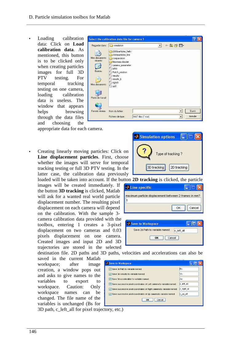
D. Particle simulation toolbox for Matlab
146
• Loading calibration data: Click on Load calibration data. As mentioned, this button is to be clicked only when creating particles images for full 3D PTV testing. For temporal tracking testing on one camera, loading calibration data is useless. The window that appears helps browsing through the data files and choosing the appropriate data for each camera.
• Creating linearly moving particles: Click on Line displacement particles. First, choose whether the images will serve for temporal tracking testing or full 3D PTV testing. In the latter case, the calibration data previously loaded will be taken into account. If the button 2D tracking is clicked, the particle images will be created immediately. If the button 3D tracking is clicked, Matlab will ask for a wanted real world particle displacement number. The resulting pixel displacement on each camera will depend on the calibration. With the sample 3-camera calibration data provided with the toolbox, entering 1 creates a 3-pixel displacement on two cameras and 0.03 pixels displacement on one camera. Created images and input 2D and 3D trajectories are stored in the selected destination file. 2D paths and 3D paths, velocities and accelerations can also be saved in the current Matlab workspace; after image creation, a window pops out and asks to give names to the variables to export to workspace. Caution: Only workspace names can be changed. The file name of the variables is unchanged (Bs for 3D path, c_left_all for pixel trajectory, etc.)

D. Particle simulation toolbox for Matlab
147
• Creating a helix displacement of particles: Click on Helix displacement particles. Again, choose either the images for temporal tracking testing or for full 3D PTV testing. In the first case, images of a sine-wave shaped displacement are created immediately. In the second case, enter the diameter of the helix, the linear distance between two points separated by one period points (interloop step) and the number of periods (number of revolutions). The images that are created and the input 2D and 3D trajectories are stored in the selected destination file.
• Adding noise: Click on Add Noise. Three types of noise are proposed on the window that pops out: A salt and pepper noise, a Gaussian noise and a speckle noise. Since one may want to add that noise on images from only one virtual camera, a second window lets re-entering the names of the designated camera. Then, depending on the type chosen, enter a few type-related specifics must be entered on the last window. For example, for “salt and pepper” noise, enter the noise density. For “Gaussian” noise, enter the mean and variance. For “speckle” noise, enter the variance. Some values are pre-entered as default values.
• Showing ideal particle trajectories: Click on Show ideal trajectories. A window allows choosing between Matlab and Tecplot graphics. An example of Tecplot ideal trajectory for 50 simulated particles is shown on the figure below:

D. Particle simulation toolbox for Matlab
148

E. 3D Particle tracking velocimetry toolbox for Matlab
149
E. 3D Particle tracking velocimetry toolbox for Matlab
E.1. Overview
Our 3D PTV toolbox for Matlab closely follows the steps and methods of the algorithm described in the main Thesis document. Only the camera calibration step is not included since it has been developed by Bouguet (2002) in his Camera calibration toolbox for Matlab. Our toolbox is designed for 3D tracking of particles from three viewpoints. The toolbox is divided into three main parts:
- Preprocessing: This mandatory step allows loading calibration data, defining images specifics such as names, size, type and number, defining particles specifics such as size of interrogation and research windows, maximum growth ratio, and defining cameras speed.
- Processing: its includes background averaging, particles centers detection after a short image processing by a weight averaging method, temporal tracking either by the polynomial regression scheme or by the modified fast-normalized cross-correlation scheme, spatial matching by the epipolar constraint method and triangulation by a least squares method.
- Post-processing: Among other features, 2D or 3D paths and velocities of groups or single particles can be displayed. Moving particles can be watched. An error analysis tool compares real 2D trajectories obtained by addition of raw particles images to 2D trajectories obtained by backprojection of the 3D trajectories data onto each camera image plane.
E.2. Getting started
System requirements: This toolbox was built with Matlab 2007b. The Image Processing Toolbox needs to be installed. The toolbox works with Windows, Linux, and Unix systems.
• Run Matlab and add the location of the folder 3DPTV_toolbox to the main matlab path. This procedure will let call any of the matlab toolbox functions from anywhere. Under Windows, this may be easily done by using the path editing menu. Under Unix or Linux, use the command path or addpath (use the help command for function description).
• From the command window of Matlab, type: PTV_toolbox The following window appears on the screen:

E. 3D Particle tracking velocimetry toolbox for Matlab
150
Start by the pre-processing steps:
• Loading calibration data: click on Load calibration data. The window that appears helps browsing through the data files and choosing the appropriate data successively for each camera. When it is done, it is asked whether the 3D reference frame where the 3D coordinates will be calculated is different from the 3D frame of the calibration target. If the user click on Yes, he will be prompted to enter in the Matlab command window, the 3x1 translation and 3x3 rotation matrices that turn the 3D calibration target frame into the work 3D reference frame.

E. 3D Particle tracking velocimetry toolbox for Matlab
151
• Defining images: Click on Define images. On the first window that appears, select the directory where the particles images are stored. The second window allows choosing images specifics: names, type, start number, end number, and number of background images that will be averaged.
• Defining particles specifics: Click on Define particles specifics. Enter the size of interrogation and research windows, as well as the maximum growth ratio for the research windows. If there is no particle in a research window, its size will be automatically expanded iteratively up the allowed ratio.
• Defining camera speed: Click on Define camera speed. Enter the cameras frame rate. The skip count permits skipping some images when performing the tracking. For example, if the frames start number is 1 and the skip count 2, tracking will be done based on images 1, 3, 5…

E. 3D Particle tracking velocimetry toolbox for Matlab
152
Now, proceed to the main processing steps:
• Averaging the background: Click on Average background. The averaging is done based on the number of background images entered when defining images specifics. The resulting background image for each camera is stored in the images file with the extension number 0. The remaining image processing steps (background subtraction, noise removal) are to be conducted by the user and are not included in the toolbox since they highly depend on the images quality.
• Detecting particle centers. As previously mentioned, a preliminary image processing to make particle visible after background subtraction must be conducted before this step. This task is not included in the toolbox. Click on Detect particles centers. The user is asked to enter a threshold level in the Matlab command window. All pixels with luminance under the threshold will be set to 0 while the other pixels will remain unchanged. Remaining noise from background is thus subtracted while keeping the Gaussian profiles of particles images at the same time. Pixel coordinates of particles centers in each image are stored in the image file under *.text format. Real particles 2D trajectories are created by adding up clean particle images and are shown on three images stored with the extension *_total. Each particle trajectory has colors ranging from blue (start of trajectory) to red (end of trajectory).
• Performing temporal tracking: Click on Temporal Tracking. By checking the radio buttons, choose on which camera images the tracking will be conducted. By pressing the button Polynomial Regression or the button Modified Cross-Correlation, the 2D tracking is launched with the desired tracking scheme. Each scheme is fully described in the main document of the Thesis. When the tracking is completed, images comparing real 2D trajectories with tracked 2D trajectories are automatically displayed for each camera. Real trajectories are colored in white while tracked trajectories are red or blue-colored, thus allowing a visual checking of the temporal tracking accuracy.

E. 3D Particle tracking velocimetry toolbox for Matlab
153
• 3D reconstruction: Click on 3D Reconstruction. In the Matlab Command window, enter a match threshold s for the fundamental matrix relation:
[ ] sy
x
Fyx p
1
1 2
2
1211
where (x1,y1) and (x2,y2) are two time synchronous (i.e. pixel coordinates of a particle on two cameras at the same instant time) normalized pixel coordinates. Ideally, the left term of the equation should equal zero but it never does, due to experimental and computational errors. s is given the default value 1.
A text file named Traj_3D.txt is automatically created in the images file. A Matlab data file named Results.mat is also created. It contains the 3D path under the variable B of each particle, the 3D successive velocities under the variable V, the 3D acceleration under the variable A, and the tracked 2D trajectories for cameras 1, 2 and 3 respectively under the variables cent_left_all, cent_right_all and cent_up_all. The format of those matrices is:
- For B, V and A: lines correspond to time frames. First three columns correspond to coordinates x, y and z for particle 1, second three columns are coordinates x, y, and z for particle 2, etc. in the calibration target 3D reference frame.
- For cent_left_all, cent_right_all and cent_up_all: First two columns correspond to coordinates x and y for particle 1, second two columns are coordinates x, and y for particle 2, etc. in the image plane 2D reference frame (pixels).
After 3D reconstruction, a window pops out and proposes to export those variables to the Matlab workspace under chosen names. Caution: Only workspace names can be changed. The file names of the variables remain unchanged (B for 3D path, cent_left_all for 2D trajectory, etc.)
What follows is an overview on some post-processing functions.
• Viewing 3D trajectories: Click on Show trajectories (PTV mode). First, one must decide whether Matlab or Tecplot graphics are desired. In the following example, Matlab graphics are used. The created graphics are:
- One plot for the 3D paths of all tracked particles - One plot for the successive 3D velocities

E. 3D Particle tracking velocimetry toolbox for Matlab
154
- For each camera: One plot of the 2D trajectories in the camera pixel reference frame and one plot of the same 2D trajectories using the camera averaged background (more realistic). Tip: Make sure the real averaged background image has the number 0 in the images files.

E. 3D Particle tracking velocimetry toolbox for Matlab
155

E. 3D Particle tracking velocimetry toolbox for Matlab
156
• Viewing 2D velocity fields: Click on Instantaneous velocity (PIV mode). Again, one must decide whether Matlab or Tecplot graphics are desired. In the following example, Tecplot graphics are used. In the window that appears, enter the frame number which is the instant time when the map of the 2D velocity vectors is wanted. The created graphs are:
- 3D velocity field at the chosen instant time. - For each camera, the 2D velocity field from image plane reference frame
Caution: When using Tecplot, one needs to be in vector mode to see the velocity field. The vector variables are U, V and W for 3D visualization and U, V for 2D visualization. One can also display the 2D velocity field with the chosen frame as background but then, Matlab graphics must be used. This scheme allows checking that all velocity vectors start points are real particle images.

E. 3D Particle tracking velocimetry toolbox for Matlab
157

E. 3D Particle tracking velocimetry toolbox for Matlab
158
• Viewing a single particle trajectory: Click on View single particle trajectory. After choosing the type of graphic, enter the chosen particle identification number in the Matlab Command window. This number is the particle position among matrix B (matrix of 3D positions) columns. Particle 1 data has first three columns of B (respectively first two columns of cent_left_all, cent_right_all and cent_up_all); Particle 2 data has second three columns of B (respectively first two columns of cent_left_all, cent_right_all and cent_up_all), etc. The created graphs edited with Matlab are:
- One graph for the 3D path of the particle - One plot for the successive 3D velocities of the particle - For each camera: One plot of the particle’s 2D trajectory in the camera pixel
reference frame and one plot of the same 2D trajectories using the camera averaged background (more realistic). Tip: Make sure the real averaged background image has the number 0 in the images files.

E. 3D Particle tracking velocimetry toolbox for Matlab
159

E. 3D Particle tracking velocimetry toolbox for Matlab
160
• Watching particles moving: Click on Play movie. The following window appears:
Clinking on Successive velocity field allows watching the displacement of a single particle or a group of particles on each camera image plane. To do so, enter the particles identification number in the Matlab Command window.
Clicking on Watch trajectories growing does the same thing as previously but with all particles at the same time.
Clicking on Raw particles images creates a movie from raw particle of each camera. This is particularly useful if clean particles images (after background subtraction and image processing) are used as inputs.
• Analysis error: Click on Analyze error. Two tasks are conducted by Matlab:

E. 3D Particle tracking velocimetry toolbox for Matlab
161
- First, it compares the real 2D trajectories obtained by addition of raw particles images, with 2D trajectories obtained by backprojection of the 3D trajectories data onto each camera’s image plane. Real images trajectories are plain white, while backprojected trajectories are blue. This is an important way to visually assess the efficiency of the overall 3D PTV process.
- Second, the position and velocity errors are computed along with the total pixel error on each camera. The ratio of mean particle spacing (in a nearest neighbor sense) to mean displacement of particles between two consecutive frames ξ is calculated for each camera based on the first two frames. For each camera, a few numbers are calculated and displayed: The number of real 2D trajectories is calculated as the number of detected centroids on the first particles image. The number of tracked 2D trajectories is calculated from the 2D trajectory matrices issued by the temporal tracking step (cent_left_all, cent_right_all and cent_up_all) without any assumption on the accuracy of the 2D trajectories. The number of real 3D trajectories is calculated as the maximum among the number of centroids detected on each camera image plane. Therefore, it is a minimum value. The number of tracked 3D trajectories is calculated from the matrix of particles 3D paths.
Here is an example of the displaying of the error data.

E. 3D Particle tracking velocimetry toolbox for Matlab
162
• Drawing velocity contours: Click on Velocity contours. This function needs dense particle seeding to yield relevant results. The 3D and 2D velocities isolines are generated respectively from the matrix of 3D particles positions B and from the matrices of 2D trajectories yielded by the temporal tracking step.
• Loading 3D PTV tracking results from previous calcuation: This function is particularly useful when the user wants to post-process results from a previous 3D PTV calculation without having to go over the whole process again. To do so, click on Load. Just like in the pre-processing step, load the calibration data files and define the images specifics. When it is done, the last window that appears helps browsing through the data files and selecting the tracking result file to be used. Select the file containing matrices B (successive 3D positions), V (successive 3D velocities), cent_left_all (2D trajectories for camera 1), cent_right_all (2D trajectories for camera 2) and cent_up_all (2D trajectories for camera 3). This file was automatically created and stored in the user’s image file under the default name Results.mat.

E. 3D Particle tracking velocimetry toolbox for Matlab
163

F. Résumé substantiel en français
164
F. Résumé substantiel en français
1. Introduction
Le suivi Lagrangien tridimensionnel de particules (en anglais 3D particle tracking velocimetry, 3D PTV dans la suite) dans les grands volumes est un moyen clé de l’étude des structures d’écoulements liés à la convection naturelle turbulente dans les pièces d’habitation. Les propriétés locales des champs de vitesse et de température autour des sources de chaleur sont encore mal connues, en dépit du fait que ce phénomène est très répandu. Les anémomètres à fil chaud généralement employés dans le bâtiment sont intrusifs et donnent une mesure ponctuelle avec de grandes incertitudes pour les flux d'air lents ascendants car les sondes créent leur propre convection. De plus, ils sont limités à 10cm/s alors que l’air intérieur est généralement plus lent. La vélocimétrie par images de particules stéréoscopique (en anglais particle image velocimetry, PIV dans la suite) produit des champs 3D de vitesse instantanée, mais uniquement à l’intérieur de minces couches laser.
La littérature montre qu'au cours des 15 dernières années, la grande majorité des recherches sur la 3D PTV ont été consacrées à des volumes allant des échelles de Kolmogorov (Virant et Dracos 1997, Sang et Seok 2005) à quelques centimètres (Suziki et Kasagi 2000). Les données expérimentales que pourrait fournir la 3D PTV de grande échelle sont cruciales pour l’amélioration de la qualité de l’air intérieur des bâtiments par l’élaboration de nouvelles stratégies de ventilation et l’étude de la propagation des polluants dans les espaces habités. La validation et l’amélioration des codes CFD (Computational Fluid Dynamics) est également l’un des buts visés.
Cependant, la 3D PTV sur des volumes supérieurs au mètre cube soulève de nouveau
défis en terme d'éclairage, de positionnement des caméras et de choix des traceurs. Les lasers pulsés utilisés dans la PTV à petite échelle (Adrian 1991, Willneff 2002, Ouellette et al. 2006) ne peuvent pas être employés sur de plus grands volumes car la densité d'énergie de la lumière diminue rapidement quand le faisceau est agrandi. Il est extrêmement difficile de suivre dans les grands volumes les particules nanométriques et microniques couramment utilisées dans la PTV à petite échelle.
La section 2 de ce résumé décrit les particules employées ainsi qu’une méthode de détection de leurs centres. La section 3 présente la méthode de suivi temporel des images de particules. La section 4 expose la procédure d’appariement 3D des trajectoires obtenues. La section 5 présente la méthode de triangulation 3D. La section 6 présente le processus de validation du système de mesure et l’estimation des incertitudes de mesure. Les résultats de plusieurs expériences avec le système de mesure sont indiqués dans la section 7.

F. Résumé substantiel en français
165
2. Détection des particules
Les traceurs utilisés sont des bulles de savon remplies d'hélium de 2 à 3mm large. Leur durée de vie est 2 mn et elles n'explosent pas lors de la collision sur le matériel expérimental ou les murs. Les générateurs de bulles commerciaux produisent environ 300 bulles/s (Anonymous 1988). En raison de leur bonne visibilité, Ces traceurs sont largement utilisés pour les d’applications dans l’air (Kessler et Leith 1991, Okuno et al. 1993, Müller et Renz 1996, Sholzen et Mozer 1996, Suziki et Kazagi 1999, Zhao et al. 1999, Sun et Zhang 2003, Machacek 2002).
Leur densité par rapport à l’air a été évaluée par Kerho et Bragg 1994. Ils ont montré que les bulles plus denses que l'air sont détruites par les bulleurs usuels tandis que des bulles de densité neutre et des bulles plus légères que l'air sont produites. Pour éliminer ces dernières nous avons introduit un cylindre à surface rugueuse au sein l’unité de production de notre bulleur car les bulles plus légères que l’air sont attirées vers le centre de l’unité par la force centripète. Kerho et Bragg 1994 ont également démontré que, après élimination des particules plus légères que l'air, les particules restantes, même imparfaitement neutres, peuvent suivre l’écoulement dans des milieux à faibles gradients de pression. C'est le cas dans le bâtiment.
Comme le montre la Figure 1, les bulles sont généralement vues sous la forme de deux (ou seulement une, en fonction du recul des caméras) taches lumineuses qui se forment à leur surface. Cela justifie l'utilisation des méthodes de calcul du de centre de masse pour déterminer les coordonnées pixels des centres des particules après suppression du fond et du bruit. Pour chaque particule, les coordonnées (xc, yc) du centre de masse sont données par :
∑∑=
),(
),(
yxI
yxxIxc
; ∑∑=
),(
),(
yxI
yxxIyc
(1)
où (x, y) sont les coordonnées du pixel et I (x, y) sa luminance.
a- b-
Figure 1 : (a)- Points lumineux à la surface d’une bulle (D’après Machacek 2002). (b)- Résultat du calcul du centre de masse sur trois particules différentes. Celles à gauche et au centre de l’image produisent un centroïde unique tandis que celle de droite en produit deux. Agrandissement x 800.

F. Résumé substantiel en français
166
3. Tracking temporel
Le tracking temporel consiste à suivre une même particule sur plusieurs images successives. En fonction de la densité d’ensemencement et de la longueur des trajectoires, deux méthodes sont employées :
- Tracking temporel par inter corrélation normée modifiée (méthode développée au CETHIL)
Centrée sur la position précédente de la particule, une zone de recherche est ouverte dans l’image suivante. Cette fenêtre a pour taille :
rn
tV+=
.maxα (2)
où Vmax est la vitesse maximale du fluide, t l’intervalle de temps entre deux images, r le rayon de la bulle et n la valeur du pixel (en m/pixel). La fonction d’inter corrélation normée s’écrit:
( )[ ] ( )[ ]( )[ ] ( )[ ]∑ ∑ −−−−
−−−−=
yx yxvu
vu
tvyuxtfyxf
tvyuxtfyxfvu
,
2
,
2
,
,
,,
,,),(γ (3)
Où f est la fenêtre de recherche, t la moyenne de la luminosité des pixels de la bulle et
vuf , est la moyenne de f(x,y) sur une région de la bulle. Les critères de recherche par
inter corrélation sont la forme et la luminosité de la bulle. En cas d’ambiguïté de tracking (pics d’inter corrélation de tailles voisines), la position probable de la bulle est calculée par extrapolation Lagrangienne à partir des positions précédentes. La bulle la plus proche de la position calculée est alors choisie.
- Tracking temporel par régression polynomiale (méthode développée à l’Université d’Illinois à Urbana-Champaign, Bio Engineering Laboratory, USA)
L’algorithme utilise un polynôme de régression du second degré pour prévoir le centre de la région de recherche :
cbtatx iii ++= 2
(4)
Où x représente le vecteur des coordonnées pixels à l’instant ti pour i allant de 1 à 5 (5 instants précédents mais pas nécessairement consécutifs). Les constantes a, b, et c sont obtenues par des méthodes de moindres carrés. La signification physique de la régression est la minimisation des changements d'accélération de la particule.
Une fonction de coût est ensuite appliquée aux particules se trouvant dans le secteur de recherche :

F. Résumé substantiel en français
167
∑
∑
=
=−−
=3
0
2
3
0
2
k k
k kk
D
HGD τφ
(5)
où Dk est le déplacement de la particule entre les images k et k+1, τk le temps entre les images k et k+1 divisé par 2, et G et H les vecteurs (1x2) constants résultant de la régression linéaire de D entre les images 1 et 4. La fonction de coût apparaît comme le résidu de la régression normalisé par un déplacement géométrique moyen. Sa signification physique est également de réduire au minimum les changements de l'accélération des particules. Ainsi, la particule ayant la valeur de fonction coût minimale est retenue.
L’inter corrélation normée modifiée est employée pour des densités d’ensemencement fortes et de courtes trajectoires temporelles (environ 10 images, en fonction de la densité d’ensemencement). La méthode par régression polynomiale a donné des résultats plus précis dans les cas de trajectoires plus longues mais pour des densités d’ensemencement plus modérées.
4. Appariement des trajectoires 2D obtenues
Cette section présente la méthode employée pour identifier dans l’espace les trajectoires vues par chaque caméra séparément. Cette méthode est basée sur le principe de la contrainte épipolaire (Mass 1992). D'abord, la matrice fondamentale liant les caméras deux à deux doit être calculée. Par exemple pour les caméras 1 et 2, elle s’écrit :
[ ] TT RRTRRTF 21221112 ⋅⋅⋅−= × (6)
avec Ti et le Ri respectivement le vecteur (3x1) de translation et le vecteur (3x3) de rotation liant le repère 3D intrinsèque (XXc) de la caméra i au repère 3D réel de travail (XX).
TXXRXXc +⋅= (7)
Les matrices Ri et le Ti sont des paramètres extrinsèques donnés par la calibration des caméras. Le produit croisé [ ]X se défini comme :
[ ]
−−
−=×
0
0
0
12
13
23
uu
uu
uu
u (8)
Suivant notre procédure, deux trajectoires sont considérées appariées s’il existe dans chaque trajectoire au moins 6 points choisis régulièrement tels que leurs coordonnées pixel synchrones vérifient :

F. Résumé substantiel en français
168
[ ] sy
x
Fyx p
1
1 2
2
1211 (9)
où (x1, y1) et (x2, y2) sont des coordonnées de pixel synchrones c’est-à-dire provenant d’images prises au même instant suivant 2 angles de vue différents ; s est une valeur seuil qui en principe vaut zéro. Cependant, en raison des erreurs expérimentales et des approximations de calcul, s n’atteint jamais cette valeur. Les tests de validations ont donnés de très bons résultats avec s ≤ 3. Par défaut s =1. Par comparaison avec les procédures traditionnelles, cette stratégie apporte un surplus de fiabilité dans la procédure d’appariement, notamment pour des trajectoires longues.
5. Reconstruction 3D
La calibration des caméras est le procédé qui permet d’obtenir leurs paramètres intrinsèques (distance focale, point principal, coefficients de distorsion et angle entre les axes des coordonnées pixels) et extrinsèques (matrices de rotation et de translation liant le repère 3D de chaque caméra au repère 3D de travail). En pratique, la calibration se fait en photographiant de différents endroits une mire de calibration plane en damier. Sur chaque image, un carré de la mire est sélectionné par l’expérimentateur. Il entre également dans l’algorithme de calibration la taille réelle des carreaux contenus dans le carré. La calibration consiste alors à minimiser l’écart entre le croisement réel des carreaux et leur croisement théorique établit suivant un modèle mathématique de la caméra.
Le modèle mathématique de caméra employé est celui proposé par Heikkilä et Silvén (1997). Il inclut des coefficients de distorsion tangentielle. La méthode d’évaluation initiale des homographies planes et l'évaluation finale du maximum de vraisemblance est celle proposée par Zhang (1999). L'évaluation des paramètres intrinsèques se fait par la méthode de l'orthogonalité des points de disparition comme présenté par Beardsley et Murray (1992).
Pour une caméra donnée, soit f la distance focale en pixels (vecteur 2x1), cc les coordonnées du point principal (vecteur 2x1), β (scalaire) l'angle entre les axes des coordonnées pixels, et k le vecteur des coefficients de distorsion radiale et tangentielle (vecteur 5x1). Soit P un point réel dont les coordonnées dans le repère 3D intrinsèque à la caméra sont (Xc, Yc, Zc). Soit xn=(x, y) les coordonnées normalisées de la projection de P sur le plan image de la caméra. Les coordonnées normalisées sont définies comme le résultat de la projection de P suivant le modèle sténopé (pinhole camera model an anglais) en supposant une distance focale unité. On peut donc écrire :
=
cc
cc
ZY
ZX
y
x
/
/
(10)
F. Résumé substantiel en français
169
En prenant en compte les paramètres extrinsèques (Equation 7), l’équation 10 devient :
iiii
iiii
i TZRYRXR
TZRYRXRx
3333231
1131211
++++++
=
iiii
iiii
iTZRYRXR
TZRYRXRy
3333231
2232221
++++++
= (11)
Nous avons donc un lien entre les coordonnées pixels normalisées et le point réel P pour chaque caméra i.
Posons r2=x2+y2. En prenant en compte la déformation due à l’objectif, les coordonnées de la projection de P deviennent :
dxxrkrkrkx nd ++++= )..².1( 65
421 (12)
où le dx est le vecteur de distorsion tangentielle de l’image :
++
++=
²)2².(..2
²)2².(..2
34
43
yrkyxk
xrkyxkdx
(13)
Après prise en compte de la distance focale et du point principal, les coordonnées pixels xPixel de la projection de P sur le plan image s’écrivent finalement :
+++
=
=
222
1211
.
)..(
ccxfc
ccxxfc
y
xx
d
dd
p
p
pixel
β
(14)
L’équation précédente peut être réécrite en:
=
111
1
d
d
p
p
y
x
KKy
x
(15)
Cette équation fait le lien entre les coordonnées pixels réelles et les coordonnées pixels normalisées.
L’équation 11 définit le calcul des coordonnées réelles par triangulation. Chaque point P du champ objet commun donne naissance à un système surdéterminé de 2n équations

F. Résumé substantiel en français
170
pour seulement 3 inconnues où n est le nombre de caméras qui voient simultanément le point P. Ce système est résolu par une méthode de moindres carrés.
6. Validation
Les capacités et la précision de l’algorithme ont été testées grâce à notre algorithme de simulation qui fonctionne comme suit : Premièrement, un ensemble de particules est créé avec une densité et un nombre choisis mais un positionnement et une luminance aléatoire dans l'espace objet 3D. Ensuite, on confère à ces particules un mouvement linéaire ou hélicoïdal dans l'espace 3D suivant des trajectoires de longueur choisie. Enfin, chaque trajectoire 3D est projetée sur le plan image 2D de trois caméras virtuelles à l’aide de données de calibration réelles. Chaque pas de temps crée ainsi une image de particules.
Premièrement un déplacement linéaire de 3 pixels par image été imposé à 2000 particules. Le ratio écart moyen entre les particules sur déplacement moyen des particules entre 2 images était en moyenne de ξ=3.7 sur les images 2D résultantes. 1841 trajectoires 2D ont été correctement restituées par l’algorithme de tracking temporel tandis que 1278 particules étaient correctement traquées dans l'espace 3D sur 40 images successives.
Deuxièmement, un déplacement hélicoïdal 3D de 5 pixels par image sur un total de 25 images a été donné aux 2000 particules, ceci afin de forcer le croisement des trajectoires 2D. Le ratio précédent était respectivement de ξ1=3.32, ξ2=2.2 et ξ3=2.88. En moyenne 1580 trajectoires 2D ont été correctement restituées par l’algorithme de tracking temporel tandis que 1659 trajectoires 3D correctes ont été trouvées. Un nombre de trajectoires 3D plus important que le nombre de trajectoires 2D s’explique par le fait que certaines trajectoires proviennent de particules vues uniquement par 2 caméras.
Dans le cas d’expériences réelles, la validation de la précision du tracking 3D s’est faite systématiquement par comparaison des trajectoires 2D réelles obtenues par simple addition d’images, avec les trajectoires 2D obtenues par projection des trajectoires 3D calculées sur le plan image de chaque caméra.
Des mesures comparatives de vitesse ont été effectuées sur une tuyère basse vitesse à l’aide de notre système de PTV 3D, d’un système PIV classique utilisant de l’encens comme traceur et un laser pulsé comme source lumineuse, et d’une sonde à fil chaud. La comparaison s’est faite sur 6 valeurs différentes de la vitesse à la sortie de la tuyère, s’échelonnant de 0.24m/s à environ 2m/s. Les résultats montrent un écart moyen de 0.062m/s entre les mesures par 3D PTV et les mesures PIV, de 0.166m/s entre les mesures par 3D PTV et la sonde à fil chaud et de 0.229m/s entre les mesures par PIV et la sonde à fil chaud.
Enfin, par des méthodes statistiques, les incertitudes du système PTV 3D ont été estimées à ±2 mm en position et ±4mm/s en vitesse avec un indice de confiance de

F. Résumé substantiel en français
171
99.7% en supposant une densité parfaite des traceurs. Ces valeurs ont été confirmées expérimentalement en déplaçant une balle de tennis de table sur des positions 3D précisément connues à l’avance.
7. Applications
L’algorithme de suivi Lagangien 3D a été testé dans une pièce de dimensions 3.1mx3.1mx2.5m à murs gris, à l'intérieur d’une cellule d’essais de dimensions 5.5mx3.7mx2.4m munie de parois noires, et à l'intérieur d'une maquette d’avion reproduite à l’échelle 1. La possibilité d’utiliser cette technique au dessus de sources de chaleur et en milieu liquide a également été testée. Pour chaque cas expérimental, le positionnement optimal obtenu pour les caméras et les sources de lumière est décrit. Il a notamment été montré que lorsque les parois du local ne sont pas noires, un éclairement indirect des particules après réflexion de la lumière sur les murs donne de meilleurs résultats de visibilité des bulles et donc des mesures plus précises.
Les résultats montrent que l'algorithme est capable de suivre plus de 1400 traceurs dans des volumes allant jusqu'à 3mx3mx1.2m. Après chaque expérience, la validation des trajectoires 3D obtenues a été faite en comparant les trajectoires réelles 2D obtenues par simple addition d’images, avec les trajectoires 2D obtenues par projection des trajectoires 3D sur le plan image de chaque caméra.
Une automatisation complète du processus de suivi 3D a été mise en place à travers le développement d’une interface graphique sous Matlab. Cette interface comprend également des outils d’estimation des erreurs et de visualisation des trajectoires.
FOLIO ADMINISTRATIF
THESE SOUTENUE DEVANT L'INSTITUT NATIONAL DES SCIENCES APPLIQUEES DE LYON
NOM : BIWOLE DATE de SOUTENANCE : 30 Septembre 2009 Prénoms : Pascal Henry TITRE : LARGE SCALE PARTICLE TRACKING VELOCIMETRY FOR 3-DIMENSIONAL INDOOR AIRFLOW STUDY NATURE : Doctorat Numéro d'ordre : 2009-ISAL-0070 Ecole doctorale : Mécanique, Energétique, Génie Civil, Acoustique (MEGA) Spécialité : Génie Civil Cote B.I.U. - Lyon : T 50/210/19 / et bis CLASSE : RESUME :
Le suivi Lagrangien d’images de particules (en anglais Particle Tracking Velocimetry ou PTV) a jusqu’à présent été principalement employé à la compréhension de la structure 2D et 3D des écoulements de petites échelles allant typiquement de longueurs de Kolmogorov à quelques centimètres. Le présent exposé décrit un système PTV adapté à la mesure tridimensionnelle de l’air à l’intérieur des bâtiments. Les traceurs utilisés sont des bulles de savon gonflées à l’hélium de 2mm de diamètre et de densité neutre par rapport à l’air. Ces particules sont éclairées par des moyens classiques de type lumière blanche continue et leur mouvement est suivi par plusieurs caméras rapides et synchrones.
La calibration préalable des caméras permet de connaître leurs paramètres internes et de définir les matrices de rotation et de translation les reliant à un repère réel 3D commun. Cette calibration se fait par des méthodes connues. Une procédure spéciale ôte des images les tâches créées par les particules se rapprochant des capteurs. Ce phénomène est fréquemment rencontré lorsque l’on dispose de peu de recul pour les caméras, comme c’est le cas dans le bâtiment. Plusieurs pics de luminance pouvant être créés par une même particule, le centre de chaque particule est calculé comme étant le centre de masse de l’ensemble des pixels constituant une bulle. En fonction de la densité d’ensemencement et du temps de suivi, deux méthodes de tracking temporel sont utilisées : La première est basée sur l’inter corrélation de l’image de chaque particule en fonction de sa forme et de sa luminance. Une extrapolation Lagrangienne de sa position à partir des positions précédemment calculées permet de lever les ambiguïtés. Cette méthode a donné de bons résultats sur des trajectoires courtes à fort ensemencement. La seconde utilise les positions antérieures du centroide pour définir une position probable par régression polynomiale. Un critère de qualité basé sur la minimisation des changements d’accélération des particules est ensuite appliqué pour résoudre les ambiguïtés. Cette méthode s’est avérée de meilleure précision sur les trajectoires plus longues mais nécessite un ensemencement modéré. Les trajectoires 2D issues du tracking temporel sont appariées sur la base de la contrainte épipolaire. Cet appariement peut se faire dès qu’une particule est vue par au moins deux cameras, ce qui augmente le nombre de trajectoires et le volume mesuré. Le calcul des coordonnées 3D se fait par triangulation suivant une optimisation par moindres carrés.
L’algorithme de suivi Lagrangien 3D a été testé dans une pièce de dimensions 3.1mx3.1mx2.5m à murs gris, à l'intérieur d’une cellule d’essais de dimensions 5.5mx3.7mx2.4m munie de parois noires, et à l'intérieur d'une maquette d’avion reproduite à l’échelle 1. La possibilité d’utiliser cette technique au dessus de sources de chaleur et en milieu liquide a également été testée. Pour chaque cas expérimental, le positionnement optimal obtenu pour les caméras et les sources de lumière est décrit. Les résultats montrent que l'algorithme est capable de suivre plus de 1400 traceurs dans des volumes allant jusqu'à 3mx3mx1.2m. Après chaque expérience, la validation des trajectoires 3D obtenues a été faite en comparant les trajectoires réelles 2D obtenues par simple addition d’images, avec les trajectoires 2D obtenues par projection des trajectoires 3D sur le plan image de chaque caméra. Une automatisation complète du processus de suivi 3D a été mise en place à travers le développement d’une interface graphique sous Matlab. Cette interface comprend également des outils d’estimation des erreurs de mesure et de visualisation des trajectoires. MOTS-CLES : Mesure des écoulements d’air, Suivi Lagrangien tridimensionnel de particules, bulles gonflées à l’hélium gazeux, qualité de l’air Laboratoire (s) de recherche : Centre de Thermique de Lyon (CETHIL) Directeur de thèse: MM. Jean-Jacques ROUX, Gérard KRAUSS, Eric FAVIER Président de jury : M. Francis ALLARD Composition du jury : MM. Francis ALLARD, Yanhui ZHANG, Jean-Jacques ROUX, Bernard LAGET, Eric FAVIER, Frédéric KUZNIK