m

NASA Contractor Report 201665

Analysis of Particle Image Velocimetry(PIV) Data for Application to Subsonic JetNoise Studies

James L. Blackshire

ViGYAN, Inc., Hampton, Virginia

Contract NAS1-19505

January 1997

National Aeronautics and

Space Administration

Langley Research Center

Hampton, Virginia 23681-0001

https://ntrs.nasa.gov/search.jsp?R=19970014309 2018-06-27T10:55:12+00:00Z

Analysis of Particle Image Velocimetry (PIV)

Data for Application to Subsonic Jet Noise Studies

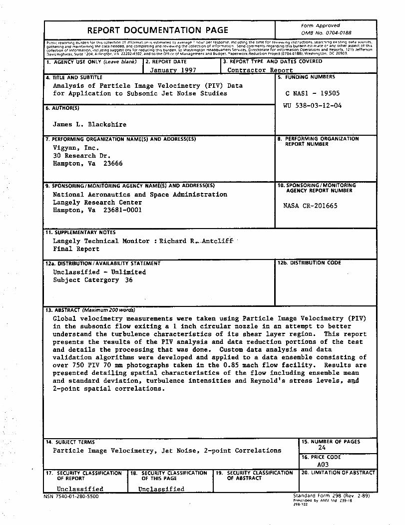
Abstract

Global velocimetry measurements were taken using Particle Image Velocimetry (PIV) in

the subsonic flow exiting a 1" circular nozzle in an attempt to better understand the turbulence

characteristics of its shear layer regions. This report presents the restllts of the PIV analysis and

data reduction portions of the test and details the processing that was done. Custom data analysis

and data validation algorithms were developed and applied to a data ensemble consisting of over

750 PIV 70mm photographs taken in the 0.85 mach flow facility. Results are presented detailing

spatial characteristics of the flow including ensemble mean and standard deviation, turbulence

intensities and Reynold's stress levels, and 2-point spatial correlations.

Analysis of Particle Image Velocimetry (PLY)

Data for Application to Subsonic Jet Noise Studies

Introduction

Global vel0cimetry measurements were recently taken as part of the Advanced Subsonic

Technology (AST) program at NASA Langley Research Center. In these measurements, Particle

Image Velocimetry (PIV) was used to measure the flow exiting a heated 1-inch circularly-

symmetric subsonic jet. The PIV technique provided spatially resolved velocity measurements in

the shear region of the expanding jet that were used to study turbulence and length scale

interaction, and their involvement in the jet-noise production process. Data was taken along a

plane intercepting the jet centerline, and included instantaneous, fluctuating, and ensemble mean

velocity, as well as ensemble standard deviation levels, turbulence intensities, Reynold's stress,

and 2-point correlations.

The specific goal of this effort was to test the feasibility of making in-situ global velocity

measurements with the PIV technique in the very harsh environment of a subsonic/transonic jet

combustor where temperatures are typically in excess of 500 degrees Farenheit, velocities range

from near zero in the entrainment regions to 1.2 mach in the jet core, and vibration and image

degradation levels can be severe. Consequently, the PIV analysis processing for this test involved

not only evaluation of the basic flow parameters, but determination of image quality levels,

measurement accuracy estimates, and data convergence evaluations.

Particle Image Velocimetry (PIV) System Description

The basic PIV measurement process involves taking an instantaneous, double exposure

record of seed particles entrained in a flow of interest.1 Two overlapping laser light sheets are

used to illuminate a measurement plane in the flow which has been seeded with neutrally buoyant

particles. Digital or photographic records of the tracer seed are then taken, where a delay is

introduced between the two laser pulses to allow the particles to move within the exposure The

local velocity, u, can then be determined from the particle image displacement measurements jn

the film recording using2:AA_

u = M (i)

where AX is the local measured particle displacement, Az is the laser pulse separation time, and M

is the system magnification.

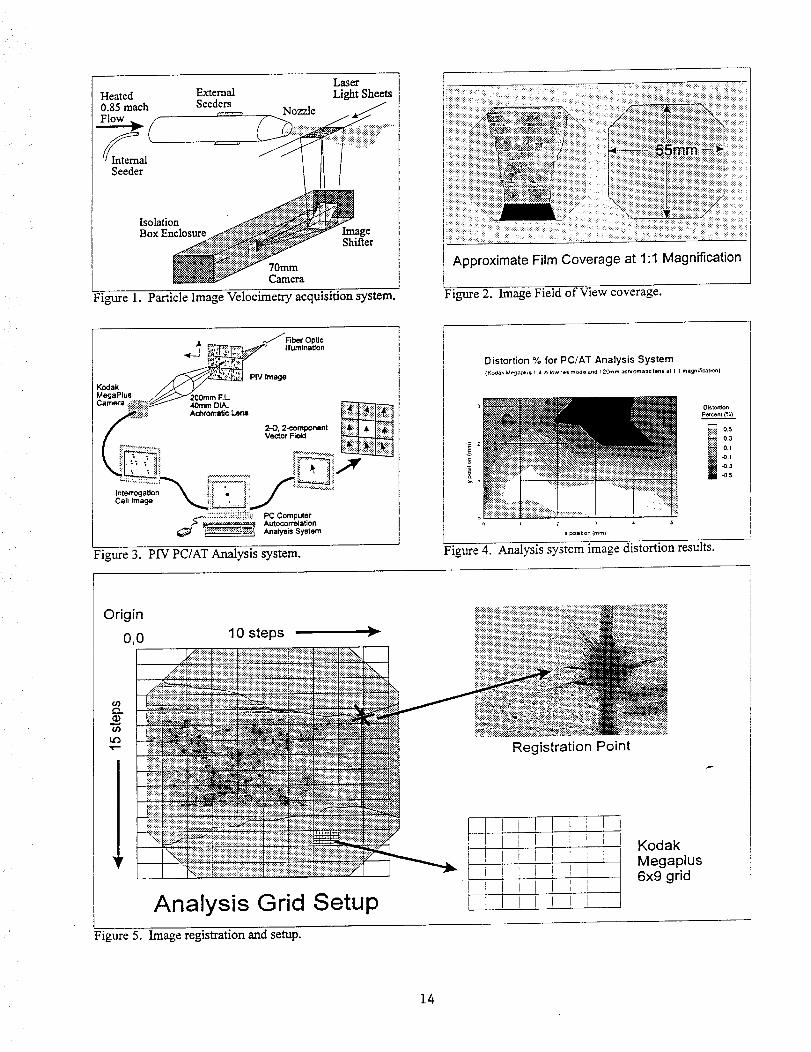
The PIV acquisition system used in this effort is depicted in Figure 1 It uses two

frequency doubled Nd:YAG lasers each operating at a wavelength of 532nm, energy of 580mj,

and 10Hz repetition rates. A 70mm Hassalblad camera system using Kodak Tri-X film was used

2

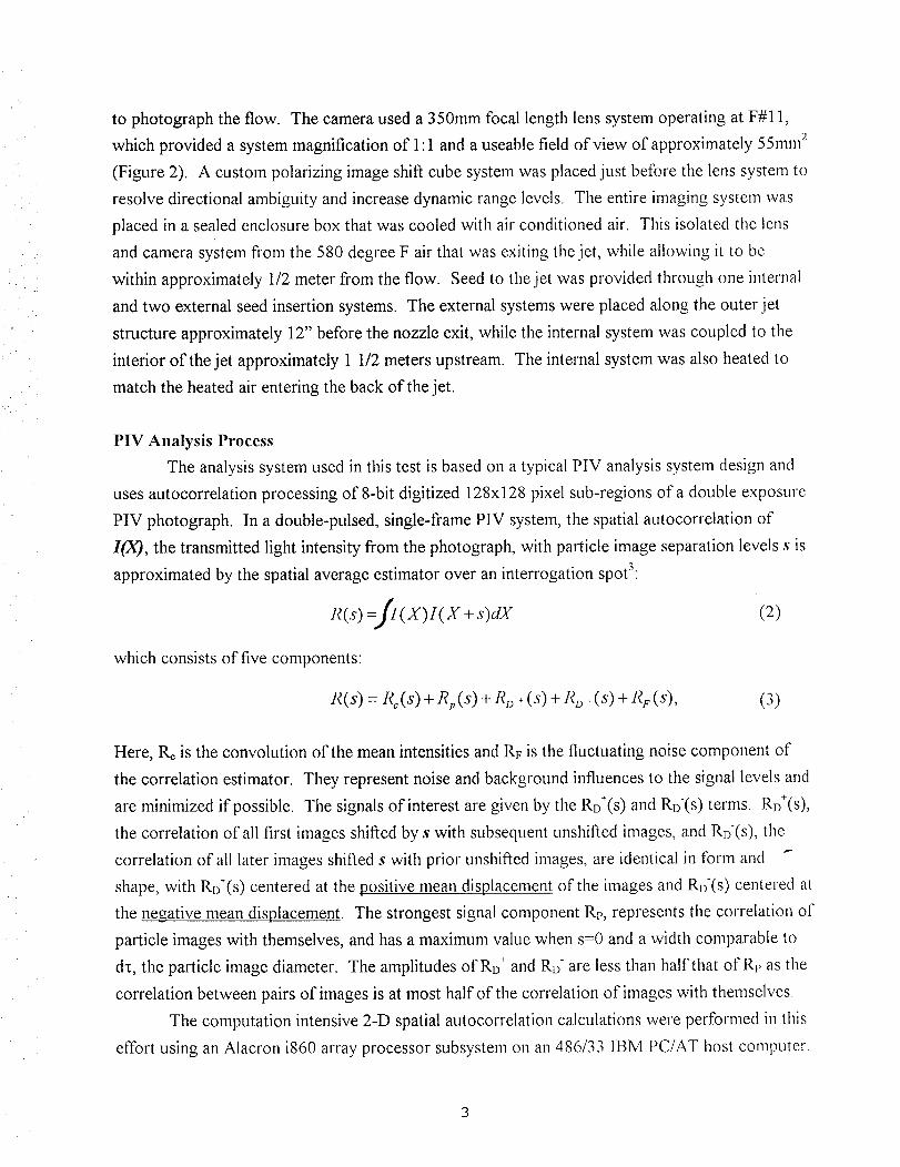
to photographtheflow. Thecamerauseda350mmfocal lengthlenssystemoperatingat F#11,

whichprovidedasystemmagnificationof 1:1andauseablefield of view of approximately55ram2

(Figure2). A custompolarizingimageshiftcubesystemwasplacedjust beforethelenssystemtoresolvedirectionalambiguityandincreasedynamicrangelevels. Theentireimagingsystemwas

placedin a sealedenclosurebox thatwascooledwith air conditionedair. This isolatedthelens

andcamerasystemfrom the 580degreeF air that wasexitingthejet, whileallowing it to be

within approximately1/2meterfrom theflow. Seedto thejet wasprovidedthroughoneinternal

andtwo externalseedinsertionsystems.Theexternalsystemswereplacedalongtheouterjet

structureapproximately12" beforethenozzleexit, while the internalsystemwascoupledto the

interior of thejet approximately1 1/2metersupstream.Theinternalsystemwasalsoheatedto

matchtheheatedair enteringthebackof thejet.

PIV Analysis Process

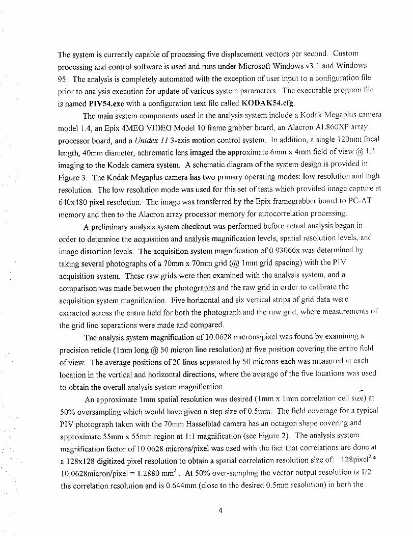
The analysis system used in this test is based on a typical PIV analysis system design and

uses autocorrelation processing of 8-bit digitized 128xl 28 pixel sub-regions of a double exposure

PIV photograph. In a double-pulsed, single-frame PIV system, the spatial autocorrelation of

I00, the transmitted light intensity from the photograph, with particle image separation levels s is

approximated by the spatial average estimator over an interrogation spot3:

R(s) =.fI(x)I(x + s)dX (2)

which consists of five components:

l (s) = IUs) + Rp(s) + +(s) + .(s) + RF(s), (3)

Here, R_ is the convolution of the mean intensities and Rv is the fluctuating noise component of

the correlation estimator. They represent noise and background influences to the signal levels and

are minimized if possible. The signals of interest are given by the RD*(s) and RD(s) terms. RD÷(s),

the correlation of all first images shifted by s with subsequent unshifted images, and RD-(s), the

correlation of all later images shifted s with prior unshifted images, are identical in form and

shape, with RD*(s) centered at the positive mean displacement of the images and RD-(s) centered at

the negative mean displacement. The strongest signal component Rp, represents the correlation of

particle images with themselves, and has a maximum value when s--0 and a width comparable to

d_, the particle image diameter. The amplitudes of Rj and RIS are less than half that of Rp as the

correlation between pairs of images is at most half of the correlation of images with themselves.

The computation intensive 2-D spatial autocorrelation calculations were performed in this

effort using an Alacron i860 array processor subsystem on an 486/33 IBM PC/AT host computer.

Thesystemis currentlycapableof processingfive displacementvectorspersecond.Custom

processingandcontrol softwareisusedandrunsunderMicrosoftWindowsv3.1 andWindows95. Theanalysisis completelyautomatedwith theexceptionof userinputto a configurationfile

prior to analysisexecutionfor updateof varioussystemparameters.Theexecutableprogramfile

is namedPIV54.exewith aconfigurationtext file calledKODAK54.efg.

Themainsystemcomponentsusedin theanalysissystemincludea KodakMegapluscamera

model1.4,anEpix 4MEG VIDEO Model 10framegrabberboard,anAlacronAL860XP arras,

processorboard,anda Unidex 11 3-axis motion control system. In addition, a single 120ram focal

length, 40mm diameter, achromatic lens imaged the approximate 6mm x 4ram field of view @ 1:1

imaging to the Kodak camera system. A schematic diagram of the system design is provided in

Figure 3. The Kodak Megaplus camera has two primary operating modes: low resolution and high

resolution. The low resolution mode was used for this set of tests which provided image capture at

640x480 pixel resolution. The image was transferred by the Epix framegrabber board to PC-AT

memory and then to the Alacron array processor memory for autocorrelation processing

A preliminary analysis system checkout was performed before actual analysis began in

order to determine the acquisition and analysis magnification levels, spatial resolution levels, and

image distortion levels. The acquisition system magnification of 0.93066x was determined by

taking several photographs of a 70mm x 70mm grid (@ 1mm grid spacing) with the PIV

acquisition system. These raw grids were then examined with the analysis system, and a

comparison was made between the photographs and the raw grid in order to calibrate the

acquisition system magnification. Five horizontal and six vertical strips of grid data were

extracted across the entire field for both the photograph and the raw grid, where measurements of

the grid line separations were made and compared.

The analysis system magnification of 10.0628 microns/pixel was found by examining a

precision reticle (lmm long @ 50 micron line resolution) at five position covering the entire field

of view. The average positions of 20 lines separated by 50 microns each was measured at each

location in the vertical and horizontal directions, where the average of the five locations was used

to obtain the overall analysis system magnification.

An approximate lmm spatial resolution was desired (lmm x lmm correlation cell size) at

50% oversampling which would have given a step size of 0.5mm. The field coverage for a typical

PIV photograph taken with the 70mm Hasselblad camera has an octagon shape covering and

approximate 55mm x 55mm region at 1:1 magnification (see Figure 2). The analysis system

magnification factor of 10.0628 microns/pixel was used with the fact that correlations are done at

a 128x128 digitized pixel resolution to obtain a spatial correlation resolution size of: 128pixel 2 *

10.0628micron/pixel = 1.2880 mm 2 . At 50% over-sampling the vector output resolution is 1/2

the correlation resolution and is 0.644mm (close to the desired 0.5mm resolution) in both the

4

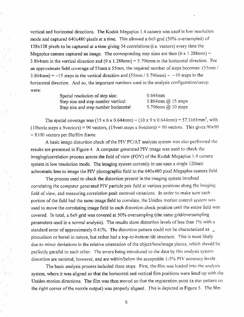
verticalandhorizontaldirections. TheKodak Megaplus1.4camerawasusedin low resolution

modeandcaptured640x480pixelsat a time. Thisalloweda6x9grid (50%oversampled)of

128x128pixelsto becapturedat atimegiving54correlations(i.e.vectors)everytime the

Megapluscameracapturedanimage. Thecorrespondingstepsizesarethen(6 x 1.288mm)=

3.864mmin theverticaldirectionand(9 x 1.288mm)= 5.796mmin thehorizontaldirection. For

anapproximatefield coverageof 55mmx 55mm,therequirednumberof stepsbecomes:(55ram/

3.864mm) -- -15 steps in the vertical direction and (55mm / 5.796mm) = -10 steps in the

horizontal direction. And so, the important numbers used in the analysis configuration/setup

were:

Spatial resolution of step size: 0.644mm

Step size and step number vertical: 3.864mm @ 15 steps

Step size and step number horizontal: 5.796mm @ 10 steps

The spatial coverage was (15 x 6 x 0.644mm) = (10 x 9 x 0.644mm) = 57.3161mm 2, with

(10horiz.steps x 9vectors) = 90 vectors, (15vert.steps x 6vectors) = 90 vectors. This gives 90x90

= 8100 vectors per file/film frame.

A basic image distortion check of the PIV PC/AT analysis system was also performed the

results are presented in Figure 4. A computer generated PIV image was used to check the

imaging/correlation process across the field of view (FOV) of the Kodak Megaplus 1.4 camera

system in low resolution mode. The imaging system currently in use uses a single 120mm

achromatic lens to image the PIV photographic field to the 640x480 pixel Megaplus camera field.

The process used to check the distortion present in the imaging system involved

correlating the computer generated PIV particle pair field at various positions along the imaging

field of view, and measuring correlation peak centroid variations. In order to make sure each

portion of the field had the same image field to correlate, the Unidex motion control system was

used to move the correlating image field to each distortion check position until the entire field was

covered. In total, a 6x9 grid was covered at 50% oversampling (the same grid/oversampling

parameters used in a normal analysis). The results show distortion levels of Jess than 1% with a

standard error of approximately 0.41%. The distortion pattern could not be characterized as p

pincushion or barrel in nature, but rather had a top-to-bottom tilt structure. This is most likely

due to minor deviations in the relative orientation of the object/lens/image planes, which should be

perfectly parallel to each other. The errors being introduced to the data by this analysis system

distortion are minimal, however, and are within/below the acceptable 1-5% PIV accuracy levels.

The basic analysis process included three steps. First, the film was loaded into the analysis

system, where it was aligned so that the horizontal and vertical film positions were lined up with the

Unidex motion directions. The film was then moved so that the registration point (a star pattern on

the right corner of the nozzle output) was properly aligned. This is depicted in Figure 5. The fihn

wasfinallymovedto the0,0 analysispositionby moving-45ramin thehorizontaldirectionand+15mmin theverticaldirection.

Thenextstepinvolvedsettingup theconfigurationfile which isdescribedin moredetail

below. Oncetheconfigurationfile wasproperlysetup,theanalysissystemprogramwas run. This

processstartedanautomatedautocorrelationanalysisroutinethat movedthefilm in a stepwise

manner10positionsin thehorizontaldirection(5.796mmeachstep),and 15positionsin thevertical

direction(3.864mmeachstep). A low resolution(640x480)KodakMegaplusimagewascaptured

at eachpositionwhere50%oversamplingprovideda9x6vector field @ a 128xl28pixel resolution

(i.e. correlation)size. Theoutputvector field includedanASCII listingof 11float numbers

representing,thehorizontalandverticalpositionof thevector,andthecentroidpositionsandpeak

valuesfor thetop threecentroidpositionsin the searchbox region.

Theautocorrelationalgorithmusedin thissetof testswasoriginallydevelopedin 1993with

two minorupgrades/revisionsoccurringin 1994and1995,respectively.Theprocessinginvolves

eightsequentialstepsandinclude:1) imagethresholding,2) defaultimagepair inclusion,3)

autocorrelationcalculation,4) zeroout DC peak,5) applysearchbox restriction,6) applycentroid

threshold,7) computecentroids,and8) write datato file.

Step1involvesthresholdingtheraw imageaccordingto aweightedmeanof the image

intensitylevel,wheretheweightingvalueis providedbytheuserin theconfigurationfile. The

valuesusedin this test variedbetween0.9and 1.05,whereraw imagevaluesabovethe productof

theaverageimageintensityandtheweightingvalueweresetto 255(themaximumbackground

imagevaluewherethePIV imagesarerecordedasblackdotsonawhite background).A setof

threevery-weakintensityparticleimageswerethenincludedin step2 in theraw imagedataarray

for discerningsaturatedor totally blackimageregionson theframe. Thisstepwasincludedto

allow void,non-seeded,andobstructedregionsof theframeto beeasilydeletedin thevalidation

processandhasno impacton regionswith adequateseedinglevelspresent.A standard

autocorrelationprocessingstepwasthenappliedto thedatain step3. TheautocorrelationDC

peakwasthenzeroedout of thecorrelationimagein step4 giventheuser'sconfigurationvaluefor

its extent. Thesevaluestypicallyrangedfrom 4-12pixelsextendingradiallyout from the centerofthe image. Step5 involvedtheapplicationof arestrictedsearchbox regiongivenuser

configurationinputvaluesfor its positioningandextent. Carefulconsiderationandtestingwas

providedin this stepto ensure1) thattheboxwasproperlyplaced,and2) that its extentsallowed

for dynamicmovementof the particlepositionsacrosstheentirefield of view. Typicalsearchbox

extentsrangedfrom +/-25 pixelsin theaxialdirectionand+/-15 pixelsin thetransversedirection,

whichcorrespondsto velocity dynamicrangesof +600m/sto -200m/sin theaxialdirectionand

+/-200m/sin thetransversedirection. Step6 involvedapplicationof auserdefinedcentroid

thresholdlevelwherevaluesbelowthedesignatedlevelweresetto zero. This levelwas typically

240 (out of a maximum level of 255). In step 7, a weighted mean centoid computation was then

applied to all the remaining correlation peaks in the search box, where correlation patterns with

areas > 100 pixels were discarded, and the top three weighted mean centroids were written to file in

step 8.

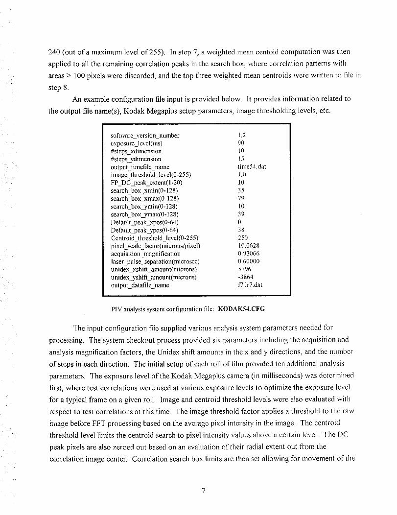
An example configuration file input is provided below. It provides information related to

the output file name(s), Kodak Megaplus setup parameters, image thresholding levels, etc.

i/

software version number

exposure_level(ms)

#steps_xdimension

#steps_ydimension

output_timefile_name

image_threshold_level(0-255)

FP_DC_peak_extent(1-20)

search box xmin(0-128)

search box xmax(0-128)

search_box_ymin(0-128)

search_box_ymax(0-128)

Default_peak_xpos(0-64)

Default_peak_ypos(0-64)

Centroid_threshold_level(0-255)

pixel_scale_factor(microns/pixel)

acquisition_magnification

laser_pulse separation(microsec)

unidex_xshift_amount(microns)

unidex yshift_amount(microns)

output_datafile_name

1.2

90

10

15

time54.dat

1.0

l0

35

79

10

39

0

38

25O

10.0628

0.93066

0.60000

5796

-3864

_ir7.dat

PIV analysis system configuration fle: KODAK54.CFG

The input configuration file supplied various analysis system parameters needed for

processing. The system checkout process provided six parameters including the acquisition and

analysis magnification factors, the Unidex shift amounts in the x and y directions, and the number

of steps in each direction. The initial setup of each roll of film provided ten additional analysis

parameters. The exposure level of the Kodak Megaplus camera (in milliseconds) was determi1_ed

first, where test correlations were used at various exposure levels to optimize the exposure level

for a typical frame on a given roll. Image and centroid threshold levels were also evaluated with

respect to test correlations at this time. The image threshold factor applies a threshold to the raw

image before FFT processing based on the average pixel intensity in the image. The centroid

threshold level limits the centroid search to pixel intensity values above a certain level. The DC

peak pixels are also zeroed out based on an evaluation of their radial extent out from the

correlation image center. Correlation search box limits are then set allowing for movement of the

7

correlation peak at various positions across the field. And finally, a default peak correlation

position is inserted in the event of a totally black or totally white image field.

PIV Data Validation

Following the analysis of all the PIV film frames, a semi-automated PIV vector validation

process was performed. These data validation efforts involved two different types of validation

processes - individual roll validation and ensemble validation. The individual roll validation

processing was done first, and involved several different types ofvalidator algorithms. Two

additional ensemble validation steps were then applied to the data that took into account the

ensemble mean and standard deviation level at each point in the flow.

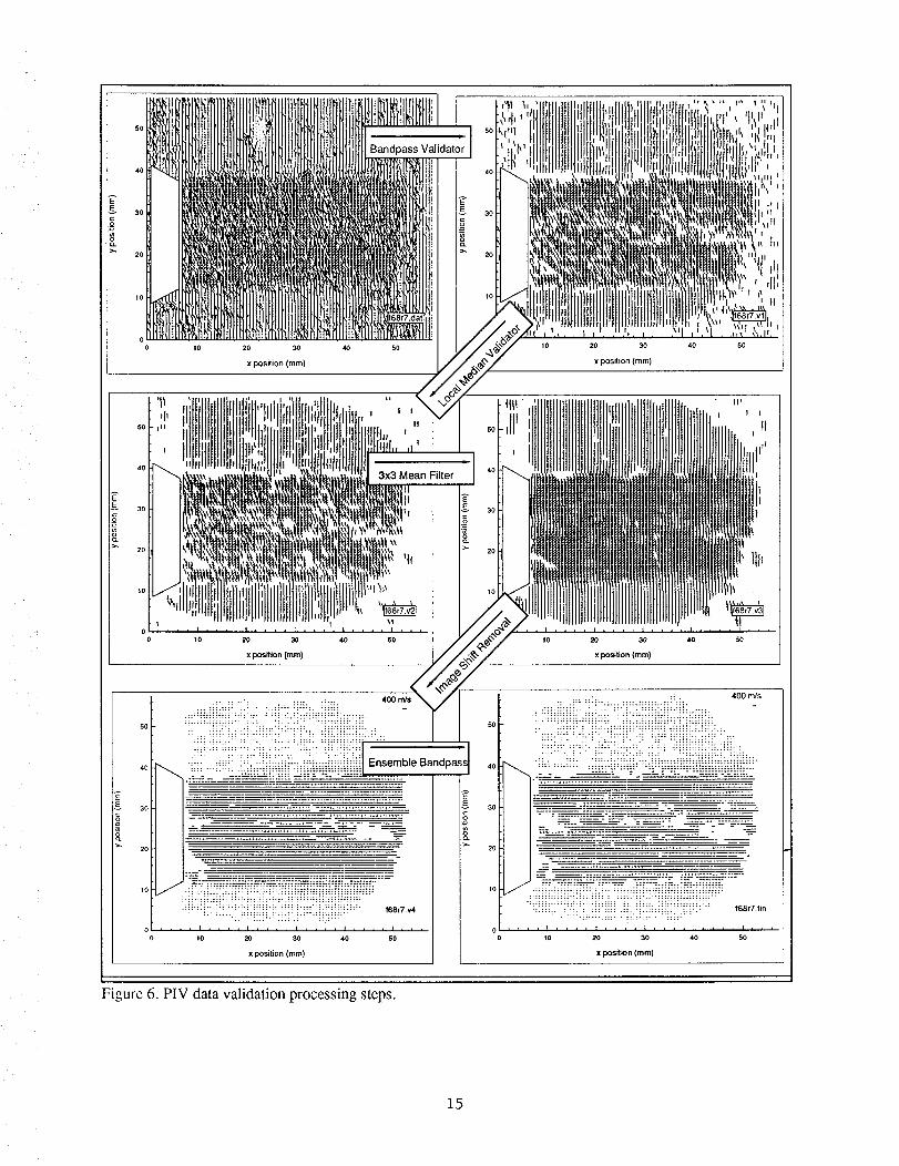
The individual roll validation involved 5 steps for the image-shift calibration fiames, and 4

steps for the actual data frames. Both the calibration and data files included a ban@ass validator, a

local median validator, and a 3x3 mean filter processor. An additional ensemble average and

manual vector validator step was then applied to the calibration files, while an additional image-shift

removal step was applied to the data files. The vector plots in Figure 6 provide a step-by-step

example of the results of each validation step from a raw data file input to the final validated file

output.

The bandpass validator was applied first, and was used to remove vectors that were

obviously bad. A set of high and low threshold levels were chosen for both the u and v components,

and if a vector was outside of these high/low threshold ranges, it was zeroed out. Unfortunately,

this step required a considerable amount of user input and judgment, and because of this, very

liberal limits were chosen for each roll of film. The executable validation program for this step was

HILO.EXE with the threshold levels being provided by the configuration file VALIDATE.CFG.

A local median validator was then applied to the data. In this processing step, a given

vector position was compared with the median value of its 8 nearest neighbors. If the absolute

value of the difference between the local median and the vector was greater than three times the

standard deviation of the 8 nearest neighbors, it was zeroed out. No user input was required for

this step. The executable validation program for this step was LOCMED.EXE. p

A 3x3 mean filter operation was then applied to the data, which involved evaluating the

mean of a vector position and its eight nearest neighbors and replacing that vector position with the

mean. This step provided a limited amount of smoothing and interpolation to the data, and like the

median validator, required no user input. The executable for this step was 3X3MEAN.EXE

An ensemble average program was then applied to each roll's image-shift calibration file to

obtain an average image shift file for that roll. The executable program for this step was

ENSEMBLE.EXE, with file name inputs being provided by the file VALADD.CFG.

8

A final manual vector extraction validation step was applied to each ensemble averaged

calibration file to remove obvious outlying vectors. The resulting calibration files were then

subtracted from each data file in an image shift bias removal step. The executable program for this

step was UNSHIFT.EXE, with file name inputs being provided by VALIDATE.CFG

Following the individual roll validation, an ensemble bandpass vatidator was applied to all

the data files, which removed vectors outside a given u and v range relative to a preliminary

ensemble mean value at each point. The determination of the threshold u and v ranges required

user input, and were ultimately chosen to be +/-125m/s for u and +/-75m/s for v. The final

ensemble mean validator compared a given vector position to a new preliminary ensemble mean

value, and if the absolute value of the difference between the ensemble median and the vector was

greater than three times the ensemble standard deviation, it was zeroed out. The executable

programs for these two steps were ENS_HILO.EXE and ENS_MEAN.EXE, respectively.

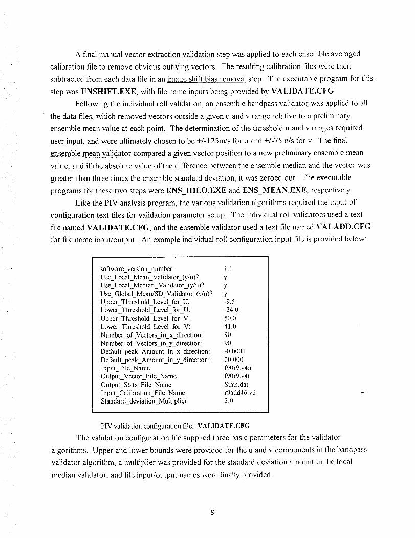
Like the PIV analysis program, the various validation algorithms required the input of

configuration text files for validation parameter setup. The individual roll validators used a text

file named VALIDATE.CFG, and the ensemble validator used a text file named VALADD.CFG

for file name input/output. An example individual roll configuration input file is provided below:

software version number 1.1

Use_Local_Mea n_Validator_(y/n)? yUse_Local_Median_Validator_(y/n)? yUse_Global_Mean/SD_Validator_(y/n)? yUpper_Threshold_Level for U: -9.5Lower Threshold Level for U: -34.0

Upper_Threshold_Level for V: 50.0Lower Threshold Level for V: 41.0

Number of Vectors in x direction: 90Number of Vectors in v direction: 90

Default_peak_Amount in x direction: -0.0001Default_peak_Amount_in_y_direction: 20.000Input_File_Name f90r9.v4nOutput_Vector_File_Name f90r9.v4tOutput_Stats_File_Name Stats.datInput_Calibration_File_Name r9add46.v6Standard_deviation_Multiplier: 3.0

PIV validation comfiguration file: VALIDATE.CFG

The validation configuration file supplied three basic parameters for the validator

algorithms. Upper and lower bounds were provided for the u and v components in the bandpass

validator algorithm, a multiplier was provided for the standard deviation amount in the local

median validator, and file input/output names were finally provided.

9

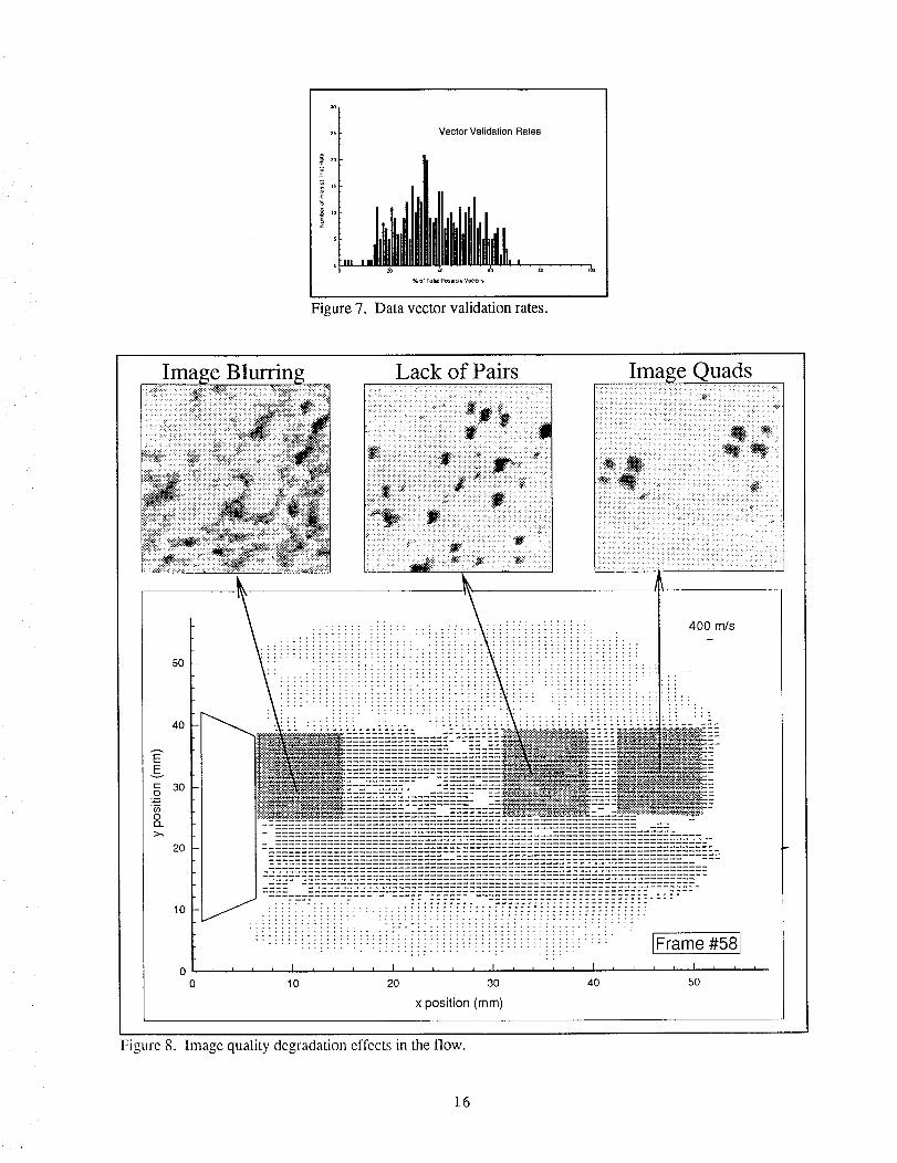
A final part of the data validation processing involved determining vector validation rates

(the percentage of actual good vectors extracted from the data relative to the maximum possible

that could be extracted). As previously mentioned, a 90x90 vector grid was analyzed for each

frame of film, which gives a total possible vector number of 8100 vectors per file. Because the

analysis grid setup (see Figure 2) was slightly bigger than the octagonal frame exposure, the

maximum vector number was actually limited to only 6935. The plot presented in Figure 7

reflects this maximum vector rate, where a 100% vector rate indicates all possible analyzed

positions produced a validated vector (6935 total vectors). Validation rates ranged from -10-

70% per file, with the majority of files falling between 40-50%, and an overall vector rate of

approximately 45%.

Results

As previously mentioned, an evaluation of image and autocorrelation signal qualities was

performed as part of this test. An initial set of low speed/cold flow PIV photographs produced

images of good to excellent quality across the entire field of view. The introduction of heat and

increased flow speeds tended to degrade the image quality, however. Some of these effects are

depicted in Figure 8. In particular, a blurring of the particle images was noticed just past the

nozzle exit, a lack of image pairs was notices in certain regions of the field, and image 'quads'

were recorded in certain regions of the downstream flow. These were most likely due to thermal

gradient, light sheet overlap, and light sheet polarization problems, respectively. The image

blurring near the nozzle exit was noticed on all of the hot/high speed flow photographs and was

consistent in its position, coverage, and effect. A lack of image pairs was noticed in approximately

1/2 of the hot/high speed photographs and 1/4 of the cold/low speed photos, and tended to be

present downstream of the nozzle. Image quads were present in about 1/2 of the hot/high speed

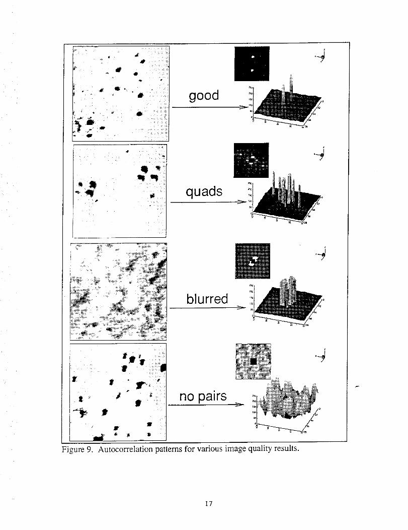
photographs and tended to be sporadically placed downstream in the main jet core. Examples of

the auto-correlation patterns produced by these various particle image qualities are provided in

Figure 9. The images with quads produced multiple correlation peaks, the blurred images

produced correlations with increased size and lowered SNRs, and the images with no pairs

produced uncorrelated results.

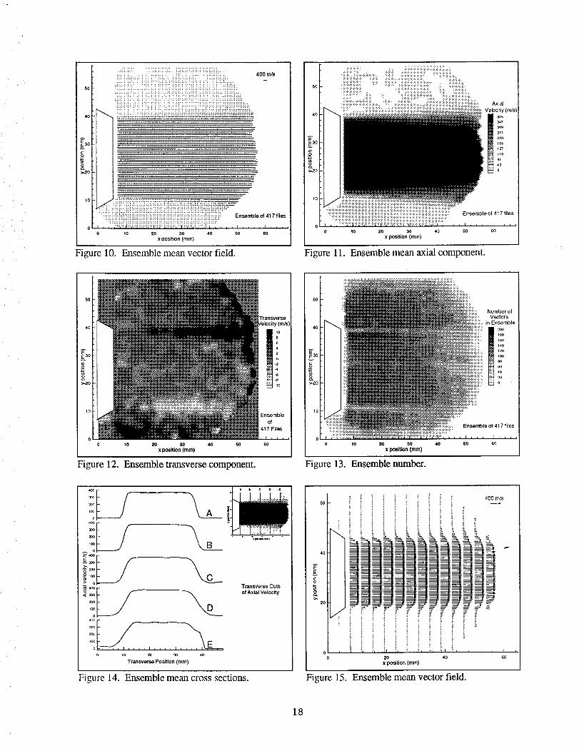
A total of 417 data files were available for ensemble and turbulence statistics calculations.

Plots depicting the ensemble mean vector field are provided in Figures 10-15. Transverse and

axial vector component contour plots are provided in two of the plots, as well as a contour plot of

the number of vectors available for the ensemble at each field point. The executable program

used in this processing step was ENSEMBLE.EXE, with filename inputs being provided by the

configuration file VALADD.CFG.

10

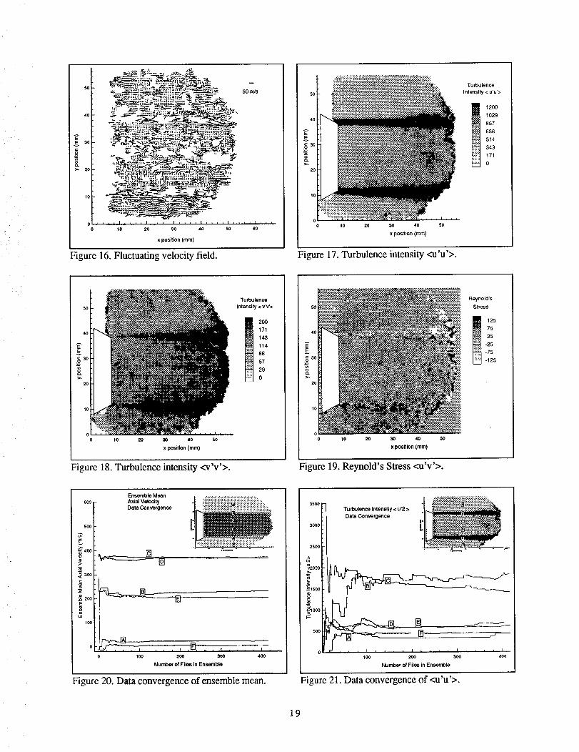
Theensembleaveragevelocityat eachpointwasthensubtractedawayfrom the

instantaneousvelocityin eachfile to produceafluctuatingvelocityat that point. Theinvolved

applyingtheexecutableprogramFLUCT.EXE to eachvalidateddatafile to produceanew

fluctuatingvelocityfile with thenewextension*.fie. An exampleof the fluctuationvelocity

output vector field is presentedinFigure 16.Severalturbulencestatisticscalculationswerethencalculatedusingthefluctuating

velocityfiles, theresultsof whicharepresentedinFigures17-19. Theyincludeplotsof axialand

transverseturbulenceintensitylevels<u'u'> and<v'v'>, Reynold'sstress<u'v'>, andthenumber

of vectorsusedin theensemblefor eachpoint in thefield. Theexecutableprogramfor this

processingwasnamedTURBSTAT.EXE.Two dataconvergencetestswerealsoappliedto theensembleaverageddata. These

includedconvergenceof the ensembleaxialvelocitymeanandconvergenceof theturbulence

intensity<u'u'>. Dataconvergencewasdeterminedfor flow pointsin the 1)entrainmentregion,2)

theshearregion,and3) thejet coreregion. Resultsarepresentedin Figures20 and21.

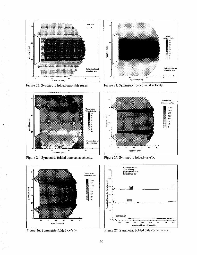
Becausethedatawastakenfrom a planethroughthejet axiscenterline,andbecauseof the

natureof thecircularnozzleconfiguration,theflow exitingthejet wasnearlysymmetricaboutthe

jet axis. Thisallowedtheensembleaverageof thedatato beincreasedby folding thedataaboutthe

jet axis. Resultsfor this increaseddataensembleareprovidedin Figures22 thin 26. In anattempt

to increasethemaximumnumberof datapointsavailablefor thefinal ensembleaverage,a slightlydifferentvalidateddatasetwasusedfor thesymmetricfoldeddatasetensemble.Thisvalidateddata

setexcludedthefinal ensemblemeanvalidationstep,thusconcludingwith the ensemblebandpass

validationstep. By doingthis,the maximumensemblenumberwasincreasedto over580in some

locations(versusonly -350 availablefor theensemblemeanvalidationstep). An additionalsetof

fluctuatingvelocityfileswerecomputedbasedon thisalternateensembleaveragefile, whichwereusedto calculateturbulencestatisticsdata. An additionaldataconvergencetestalsowasperformed

for theensemblemeanof thisnew datasetandis providedin Figure27.

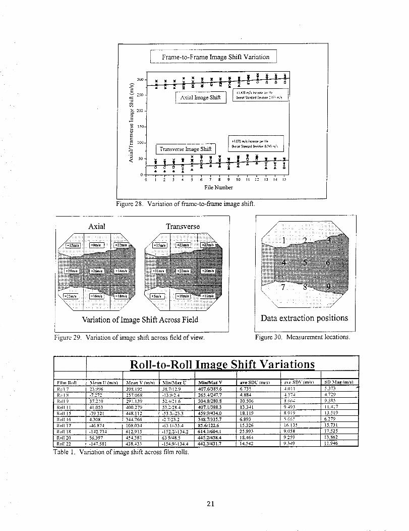
Somefluctuationsof the imageshiftbiasbeingintroducedinto thedatawerealsonoticedfrom film roll to roll, andfilm frameto frame,whichcouldhaveaneffectondataquality. A study

p

of the amount of fluctuations present, and their effect on the data was consequently done the

results of which are presented in Figures 28 thru 30 and Table 1. The Frame-to-Frame variation

is depicted in Figure 28 for film Roll #9 which had 15 calibration shots to work with. The axial

and transverse image shift values are shown for 9 positions (see Figure 30 for the relative position

locations) and showed a positive linear relationship as the frame number increased An

approximate 1.5m/s increase was noticed from frame to frame. A study of the variation of image

shift across the field of view using the same 9 points (Figure 29) indicated absolute variations

ranging from +5 m/s increase in the lower left corner position for lhe transverse component, to +

11

28 m/s for the left axial component position. No real patterns could be discerned. Roll-to-Roll

variations are shown in Table 1 where the average standard deviation of each roll was computed.

These standard deviation values ranged from 4.88m/s-25.9m/s for the axial component and

4.01m/s to 16.14m/s for the transverse component. Average standard deviations of 13.48m/s and

8.5 l m/s were computed from these values, respectively. This gives an average standard deviation

magnitude of" sqrt(13.482 + 8.512) = 15.94m/s, which gives an indication of the errors being

introduced by the image shift, in that the ensemble mean of these calibration frames were used for

data reduction, and deviations away from this mean were also present in the data sets. This

provides an error estimate due to the image shift variations of 15.94/385 = 4.14% relative to the

maximum velocity range of 385m/s in the flow.

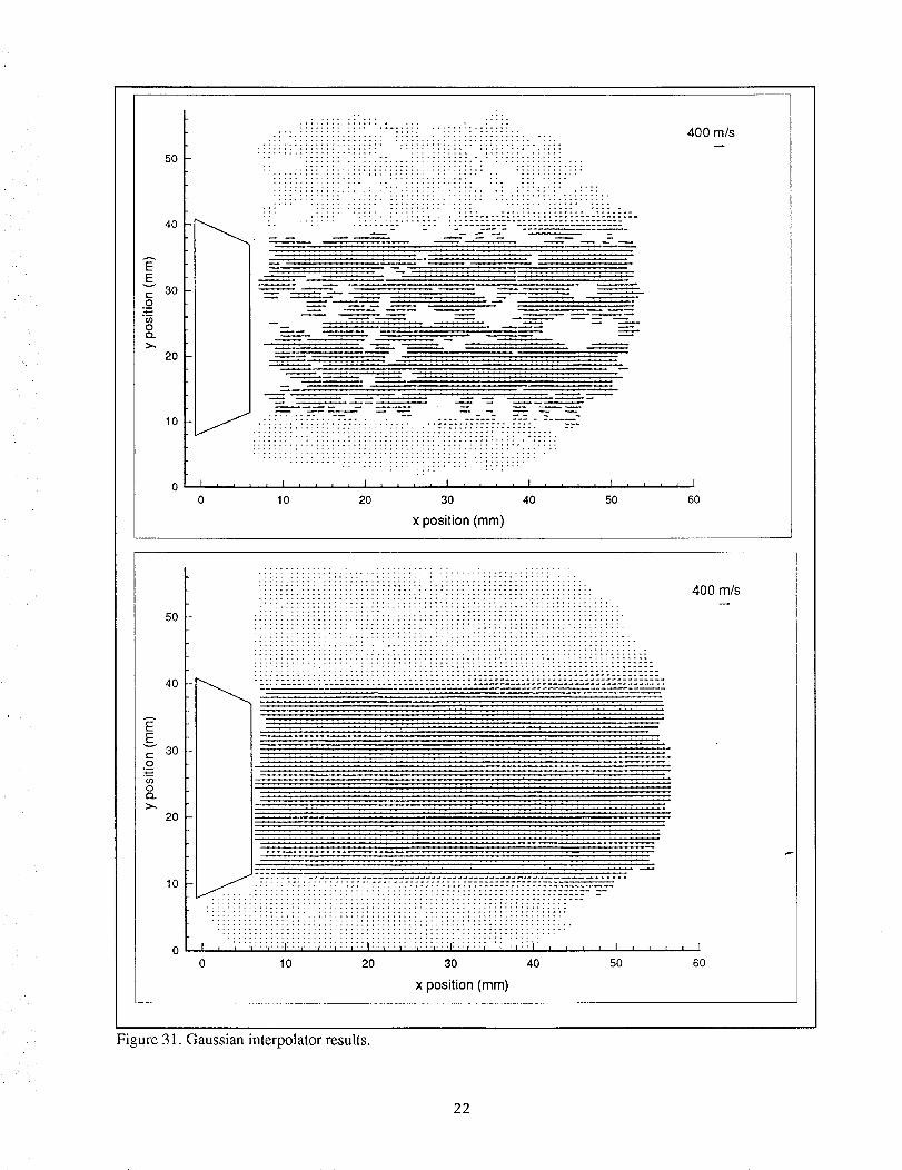
Because vector validation rates were only 40-50%, a gaussian filter/interpolation algorithm

was developed and applied to the available 417 data files. The algorithm applies a gaussian

weighting function for positions in the vector field that do not have vectors present, and uses the I0

nearest neighbors for interpolation. The gaussian weighting gives vector positions close to the

center position strong weighting in the interpolation process and positions further away less and less

weighting according to a gaussian profile. Vector positions that have valid vectors are not su[!iected

to the interpolation/filtering operation and are left unchanged. The program took the final validated

data set (*.fin) as input and output the results in files with the extension *.gfn. A new set of

fluctuating velocity files was evaluated using these new interpolated files and were given the file

extensions *.gfl. An example of the gaussian interpolator is presented in Figure 31 where the

original *.fin file is shown at the top of the figure and the gaussian filter/interpolator output is shown

on the bottom.

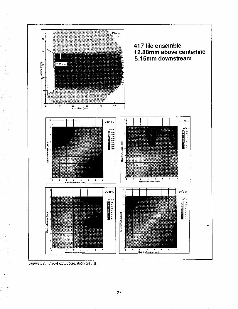
A 2-point correlator algorithm was finally developed and applied to the gaussian

interpolated fluctuating velocity files for several positions in the shear region of the flow. The

algorithm calculates 5 NxN matrices according to <u'i u'j>, <u'_ v'j>, <v'i u'j>, <v'i v'j>, and <ij>,

where i and j go from 0 -o> N, u' and v' represent the fluctuating velocities at neighboring

positions in the flow, and < > represents the ensemble averaging process. The algorithm takes the

input from a configuration file named 2PTCOR.CFG, and has an executable file name of

2PT_COR.EXE. The 2-point correlations were calculated for a position in the upper shear

region of the flow corresponding to 12.88mm above the jet centerline and 5.15ram downstream of

the nozzle. Results are presented in Figure 32.

Summary

Over 750 70mm PIV photos were analyzed in the subsonic flow exiting a 1" circular

nozzle in an attempt to better understand the turbulence characteristics of its shear layer regions.

Custom data analysis and data validation algorithms were developed and applied to a data

3_2

ensemble.Resultsarepresenteddetailingspatialcharacteristicsof theflow includingensemble

meanandstandarddeviation,turbulenceintensitiesandReynold'sstresslevels,and2-pointspatialcorrelations.

AcknowledgementsTheauthorwishesto thankW.M. HumphreysandS.M. Bartramof theMeasurement

ScienceandTechnologyBranchfor providingthePIV 70ramphotographs,andfor assistanceand

guidancein developmentof thevariousalgorithmsusedin thiseffort. Thanksarealsoextendedto Dr. J.Seiner&the Aero Acoustics Branch, and Dr. M. Glauser of Clarkson University for

their guidance and assistance with the nozzle, flow characteristics, and development of turbulent

statistics software.

References

[1] Adriane, R. J., "Scattering Particle Characteristics and Their Effect on Pulsed Laser

Measurements of Fluid Flow: Speckle Velocimetry vs Particle Image Velocimetry," Appl.

Opt. 23, 1690 (1984).

[2] Liu, Z., Landreth, C.C., Adriane, R.J., and Hanratty, T.J., "High Resolution Measurements of

Turbulent Structure in a Channel with Particle Image Velocimetry," Exp. Fluids, 10, 1991,

301-312.

[3] Keane, R.D., and Adriane, R.J., "Theory and Simulation &Particle Image Velocimetry,"

SPIE Vol. 2052 Laser Anemometry Advances and Applications, (1993), p477.

[4] Yao, C., and Paschal K., "PIV Measurements of Airfoil Wake-Flow Turbulence Statistics and

Turbulent Structures," 32nd Aerospace Sciences Meeting and Exhibit, Reno, NV, January 10-

13, 1994.

[5] Humphreys, W.M., Bartram, S.M., and Blackshire, J.L., <<ASurvey of Particle Image

Velocimetry Applications in Langley Aerospace Facilities," 31st Aerospace Scie,ces Meetin L,

& Exhibit, AIAA 93-0411, Reno, NV, January 11-14, 1993.

13

Heated0.85 roach

Seeder

Laser

External Light SheetsSeeders /Nozzle

/

Isolation

Box E_ e

_ Camera

Figure 1. Particle Image Velocimetry acquisition system.

::i:_ i:i:! !:!:i:!?i:L:::i:

Approximate Film Coverage at 1:1 Magnification

Figure 2. Image Field of View coverage.

.,_ /Fiber Optic

,.,,:¢7 _ Illumination

Kodak _IV Im

M_;aF'_us.J_'_..-_2OO,,mF.t_uame_ :_.?.__-_ 40ram DIA.

.............Si?_i!.. Actl¢omatic Lens 2-O, 2-component __::::::_ tilVectJo t Field t

!il ..'.." _|ii ii__.ii_

ii. /" ................,_--_ PC Coml_uterAutocorr_ation

Figure 3. PIV PC/AT Analysis system.

Distortion % for PC/AT Analysis System(Kodak M ,,_aplu s i 4 _ low res mode and 120mm acrwomatlc lens al 1:1magni_catm¢_)

"i ::':::::::::::::::::5:

11• position {ram}

DistortionPercent (_)

_ 0.5

0.3

0.1

-11.1

-0.3

-_L5

Figure 4. Analysis system image distortion results.

Origin

0,0 10 steps

(1"6,

_r

Analysis Grid Setup

Registration Point

KodakMegaplus6x9 grid

Figure 5. Image regisla'ation and setup.

14

..=.

/.:_iTi:_iiii!i_;i!7'!_,71i_!_Tii!i!;_i!i!ili!!i!ili!i!!!iii_===========================================================

:_!!!!:i2572!i!_iil;iiii?ii;!!i!il;i_aiZi_)2iiiii;s:_-_rT._,.... I_**lJll,lJtlllJllll[,ll

10 20 30 40 50

x position (mm)

5o

4O

3O

2O

00

.--.--_.__

J :-;'_i'_i::!!iii',!!i!i:;;i!:;:_!!_ii_iiii!_ii!!i!iiiiiiiiii!!_!__,i!iii:::i:!!iiii;iiii:ilili_,!i!i!ili:.iiii}i!,iii_i_:_ ,_r,.,o

1 I , , I r * , * _ .... I .... I .... I * , ,

tO 20 30 40 50

X position (mm)

Figure 6. PIV data validation processing steps.

15

Vector Validation Rates

Figure 7. Data vector validation rates.

Image Blurring _

ii ! !!iil............Lack of Pairs Image Quads

ii!:!_iiiiiiii!!!!!ii:i!:iii_iii!i_iiiiiiiiiii!ii!ii!i;iiiii!:i_!ii:iii!!!ili!i!iiiiiiiii!iiiiiiiiiiiiiiiii!iii!i!iiiiiii!iii

i_:,!!!iiiii_iii!iiiiiiii!iiiiiiiiiiiiiiiiil/iiii!i_ili!iiiiiliiiiii!i_iiiii_ii%i

i_ii:!!!'i::_!iiii'_::_:i!:'_:::_i_i!iii:_i_iii!ii_!!%ii'::,;iilNiil

.... iiii:::::::: i!}i::.:::::!il iimiii)i{!ii ..: i.].... i 00m/s

: :!:_._.: "_"_-: _-_" "---- ................ _ ...:.:.:-...:.:.:.:.:.:.:.:.:.:_._.:.... _._.,-_,m ._--" :::_'.'._. ._." ".'"'" , ..................... ._._..,_. :::::::::.:::&.::._.:_..-_-_._----_,,'z..,_._>:*:.,_.._..'_._-

E...... ......................... ............... _.................. _.,. _,_,_._.._...,,,_-.- - - - _ ..............:'-:er-" 30 _ :_::::"_"_":_'_ -- - ----- - -" -" _ " - - -- -_X -- - -" - ---_ _,_:::: "-'_-""_-_-'_:'_'_ ::::_ " - ----- _'_'_'_'_" "_'_ _

/ ]_.._._:._ .................. -,._-_-_::_:_+÷._: ::::-_-,+..... ÷:,_._+._:_ -

__°_O_o_N__-----------------==----------_:_:_:_j_-__----___:_ ........_-"_-_:

::iii!i!::!i::i::!::!iiiiiiiiiil)iiii!}i)ili:::::: ::iiil)il ! ii: [Frame #58

0 , , , , I , , , , I , , , , I , , , , I , , , , I , , ,0 10 20 30 40 50

X position (mm)

Figure 8. Image quality degradation effects in the flow.

16

L

G

i Q • A

J

•"_:'...... .f:. _*:..... =====================.II:I"-,;T_J :i)i.i ::_?_::_!i:--.:_::ii!!i_i,._

_"_!i!_.... :ii_: _:_,/:;':

....:":_i_:...". .... .i_:: ...: _!.: ;.;:_i_::::i:!_:_..._:

_!_! ....._ .... .:_!!_,.._£_?..--..:...,_:_!.

_:ii:':':"::_:Eiii.: " . ..@:: "':_:":':"" _:_"" .-.: ..-;_. .:..:...:::..... "::_:.-. • _::::..... • " ..._.. "::i"_:!" :_:"

:..,::::'- +..,_,..... -::_.'.'::::_:.:::'"-'-'-" . _:.:::._-'.,

_ _- %*_:_:...::.;....:_,..-_ ...f_:....._:: "%

..........._: ..........." ..i.;b.!:N:!: •..........i_:_:i" ..,.-!.........._.

T "_:

i .t

BJr

._j_

quads

blurred

no pairs

4

4

Figure 9. Autocorrelation patterns for various image quality results.

17

5o

4O I-

_30 _-

o

.:EiEEi:_,ZT!:EE!!!!iLiiiii_i:EEiliE'iEiiii6i:.:.::..::: : :::..:::::::: .-::::::::::::.:-:::::::::: 4oom/sEi,iiii!_:i:.i.il i.:.Eiii.i..EEiiiiiiiiEEi.i....iE:i6iiE_S:.

!))):_:):)))L))):):):)):)_)))))i)_)))ii))))i))i)))i)))))i))iiiii)ii)))_L....................................................................

II

i

================================================================

<::)_iiiii.)ii)i))iiii)ili)!iiiiiii)gggiiiiiiiiggggiiii_iigii_gg_=-===================================================================En_mble of 417 fil_

::::::::::::::::::::::::::::::::::::::::::::::::::::::::::::::::=============================================================

O 10 20 30 40 50 60

xposition (mm)

Figure 10. Ensemble mean vector field.

't_'•

so _ )L

,o \ m__lthyelocity(m/s)

_30 2

_ .4

>-20 -io

l°LI __E' ....... '"'"< _)" _i_ Ensemble

0 •10 20 IN) 40 _ 60

x position(mm)

Figure 12. Ensemble transverse component.

50 k-

4O _-

_o

IOF

iiiiiiiiiiiiiiiiiiiii_:'.............,::_?i!iiiiiliiiiiiiiiiiiiiiiiiiiil:ii_:=::_iiiiiii!iiiii....

iiiiiiiiii,, ,, ii•

o I

Figure 11. Ensemble mean axial component.

Axial

Velocity (m/s)

I 3e5

3O9

195

81

43

J......

:::::::::: :::::::::::::::::::::::::::::::::.:::::::5::::::::::::::::::::::::::::::::::::::::::::::::::::::::::::::::::::5::. Ensemble of 417 files• ::::::::::::::::::::::::::::::::::::::::::::::::::::::::::::::::::::::::::::::::::::::::::::::::::::::::::::::::::::::::

I , _":;:::,:;i:,:i::,i;:!:_:_:_:!;!:!:::._:_:_:!_!:!_:!:!_:_:_:!:!:_.::_:_:_:_:_:!::.i+::_!:_T_ ,, , _ .... ' ....0 I0 20 30 40 50 60

X position (rnm)

i-

,_ )::_);iiii'::::_"_ :::::::::::::::::::::::::::::::::::...................._:_!it-_%_L.:._i:_:!:i:_:_....

i :_i_:_ _ _!_:._:_:_:_:_:_:i ....

so _:i_ _ _._,_,_i-:i:i:i:i:i:i:i::i::::i:::::::_.....

__-_._!_ii:;:i:i ..... Numberof

J _ __(..i:_:i:i:S:;:_:i:i:.. in Ensemble

=========================_so

= _ - _:_ "::_::::::E:E:i:i:i:i:::.. _o

.............i.ii::::.::U!i.:-:-_: ":':"""::_i:'-:i:::!:!:!:?: _o'"_ ._iE.:Ei:i:i:i

o , , , .,, ....i,.....,.....,................_._!_i_;_i;_;.:::_i_:_::,:_:_7.............0 10 20 30 40 50 60

xposition(ram)

Figure 13. Ensemble number.

6200

1oo

o

3o0

loo

o

_oo Transverse Cuts

_oO_,o__ _D of Axial Velocity

4oo_

o . , ) .... t .

o 1o 2o 3o 40

Transverse Position (mm)

Figure 14. Ensemble mean cross sections.

o_

2

6}!i_!;i)i 400m/s

::::::::::

:::::::::::

iiti Litikk

iiiiiiiiii):

! " _' _' "' _' "' "' !_ :' ' s_o2O 40

x position (mm)

Figure 15. Ensemble mean vector field.

18

_" 40

3o_

"°IE:_ 20

10

0

0

,,.';,33-_;,:=-_._ =

.... I .... I,,

_,L_=,_-_ _'__.__::_,.:a-_ _.__ 50 m/s

===:", : . ,.a...-.r:..'._

30 40 50 60

x position (mm)

Figure 16. Fluctuating velocity field.

5°I,o

_ 3°l

20

10

0

0

i_!_!_:!:!:[_i_!_!:!:i.:i?:...:....::.::_:::;_$!_!:_$_$i._i_.:.:.::_::.:.._:_.'::!._:_.._..._:__.*:.:%%..._..:.:..-..-..-....:.:.:.:......*:':_%'%ii..-..-..-....:..-_::%i,..-..:..::..:._J_:ii._i_:_.:.'._:. .:-i-_ii_i_ii_i-.-:'.::'.:.-'_!!!_i.:".._i_i!i_!_,:.'.'_ii_i_i_:.__::':_:_:!-:'-:':_:i:_:!:_-:.:_:-:i!_!!_:.:_gi;.:ii:i:i:F.:_:_:_:_:!:_:i:__!!._

i'10 20 30 40 50

X position (mr'n)

Turbu_nce

Intensiff < u'u'>

I 1200

1029

857

686

514

343

171

0

Figure 17. Turbulence intensity <u'u'>.

I- ..i:!._.-'._ "._'_s _,.,_..._ _._:.I. ....... Turbulence

so [-- Intensity < v'v'>

,°[_-- i "'

143

=" 114

g 30 57

o_ _ 29:_ t o

20 i

_o__.:

xposition(mm)

Figure 18. Turbulence intensity <v'v'>.

.':::::.y.._::::::: ._.<.-::::_:;-'E_:k¢_..:. _..<-:::_:_!-?-?-!_::.:_:!:

..................... _,:.- • .:... ................_....:................::::::::::::::::::::: _ ._._. .. . _.::_:_.:.:::::::::::::::::::::::::::-:<-:-:-:-:-:-:¥:-:-:-.._._--'::-:_:':4:.. • :-: " _." _"_,:::::'2:_:::.'.._..: Reynold's........-..:::.:::..._.:::.:::..:_-__ _..':_..'................

50 ":::":'::::':::- :'::: ";::_ _ :'::::::" _':'::_!:'::_.":-:_ _'_:'::':_:::::':::--'::_:+'.':'.'."._'.- _ _ _F,-Y'::::.<: _-.'_: :::::,'::'_::::::.'::::::::: ". "::_:i:_:!:.::':_

" ":':-:" " .@_ _" ._-'.-'.':'_:::_"_.:_i

_ _,. .......c 30 .:::::.::. e-:.. : _ _:_....:i:i:i -125

o :_:i_ .:',:-..:::"._:..:iio. ._. _.. :-: • :::_:_:_

:>"20 " ":':" " _'_ii:.ii

10 _:i_i

-_..-.._:..."_.:.:/._]_i-i_0 :";;:_ '

0 10 20 30 40 50

x position (mm)

Figure 19. Reynold's Stress <u'v'>.

Ensemble Mean

6oo Axial Velocity

I Data Convergence

500

3oc

_ •_ -

E

. .-:-;.;-;-;.;..:...:.:.:.;.:.:.:.:.:.:.:.:.:.:.:.:.:.:..

1 "

Number of Files in Ensemble

, i , ,

4oo

Figure 20. Data convergence of ensemble mean.

i Data Convergence3000 I"

-- _$..-¢_$..

p-

100 200 300 400

Number of Files in Ensemble

Figure 21. Data convergence of <u'u'>.

19

400 m/a

E

Foldad data sol

about jet axis

J.

0 20 40 60

x position (ram)

Figure 22. Symmetric folded ensemble mean.

60-_i_iiiiiiiiiii:i::ili_i_iiiii_i_iiiiiiiiiii_ii_ii!iiiiiiiiiiiiiiiiiiiiiiiii_i:iiiiiiii_:_i_:

iiiiiiiiiiiiiiiii!i! ii!!i iii iiiiiiiiiii i iiiii iiiiiiiiiiiiiiiii!i!ii!!iii iiiiiiiiiiiiiii i ! .....

4O

E?_o

>,2o

Axial

Velocity (mls)

i s7

4_

s

..... _iii!iiiiiiiiiii!iii_iiiiiiiiii_iiii_iiiiiiiiiiiiiiiiiii_iiiiiiiiiiiiiiiii_i_iii_i_i_!_i_i_i_i_i_i_i_i_i_!_!_i_!!i!i!i_i_i_i?.

about jet axis

- _:_i_:_:_i_iiiii_iii!ii::iiiiiiiiiiiiiiiiiiiiiiii_:_::iii_i_i_::::i_i_i_i_i_:_::

o

0 20 40 60

X position (rnm)

Figure 23. Symmetric folded axial velocity.

60 . ,_"

Transverse

voio=ty(m/s)

li°p,

_ ._,:_

_0 ..................-,#i!N ,o

• _:!:...:.:$!:;....-_$_$_:.::_$!:...:.:::.i:_:_:x-...::!:;:..-:i:::..-..::T_::,

t ___':: ._ Foldad data se

.-:_iii;::ii_ii_'::i_:i:;ii;i-:ii::i::iiii::::'..:.:_':_ .... about jet axis

0 20 40 60

x position (ram)

Figure 24. Symmetric folded transverse velocity.

6O

50

_- 40

g

20

10

10 20 30 40 50

X position (ram)

Turbulence

Intons_y < u'u'>

I 1200

1029

857

686

514

343

171

0

6O

Figure 25. Symmetric folded <u'u'>.

60

Turbulence

Intensity < v'v'>

171

143

t14

86

57

tO 20 30 40 50 60

x position (ram)

Figure 26. Symmetric folded <v'v'>.

SO

o

30

_ _o

ul

lO

Ensemble Mean

Axial Velocity

Data Convergence

Folded Data Set

[]

.... ,,,, ,,, .....................

100 200 300 400 500 600 700 800

Numl_er of Fite_ in Ensemble

Figure 27. Symmetric folded data convergence.

2O

I Frame-to-Frame Image Shift Variation

300.

250.

.=

_-0 200

,_ 150

e"

"_ 50-

Axial Image Shift e,e_o, slo_o,d 0_,,_, :177 _/_

*-1.670m/s hcteose_ file

[ Transverse Image Shift ] 0vcf_ Stondofd0_'ot_ 8.745 m/_

0I i I i I I 1 I

. ll3 ll4 i[50 l " 3 4 5 6 _ $ 9 llO 11 1'2

File Number

Figure 28. Variation of frame-to-frame image shift.

Axial Transverse

Variation of Image Shift Across Field

Figure 29. Variation of image shift across field of view.

Data extraction positions

Figure 30. Measurement locations.

Fihn r.II ] Mean U (m/s)

Roll 17

Roll-to-Roll Image Shift Variations

,Mean V On/s) .Min/Max U Min/Max V

-46.874

ave SDt; (.,/s'_

6.735

ave SDV (m/s) SD Ma_ (nv's)

5.373Roll 7 23.996 398.195 38.7/12.9 407.6/385.6 4.011

Roll 8 -7.272 257.068 -13.9/2.4 265.4/247.7 4.884 4.574 4.729

Roll 9 37.210 29 I. 139 52.4/21.6 304.8/280.8 10.506 8.664 9.585

Roll I I 41.053 400.279 53.2,28.4 407.1/388.3 13.341 9.493 11.417

Roll 15 -39.321 448.112 -53.3i-23.3 459.9/434.0 18. I 19 R.919 13.519

Roll 16 4.308 344.766 -2.7/23.2 348.7/335.7 6.893 5.665 6.279

15.326 16.135 15.731t08.034

612.915

454.381

438.433

Roll I8

-63.1/-35.4

-152.2/-134.2

63.9/48.5

-154.9/-134.4

-142.734

85.6/122.6

614.1/604.1

445.2/458.4

442.3/431.7

56.397

25.993

18.464

14.542-147.581

9.058

9.259

9.349

Roll 20

Roll 22

17.525

13.862

11.946

Table I. Variation of image shift across film rolls.

21

50I

40 I-

E

c 30 I-.o

¢,3

0

2O

:: .... ::i?!:!;i!iii:i!iiii_ii:: ;!i::;;i!:. :!;i;!i!i:!!:::::: :::::::'::: • ::::::::::::. ::. ::: ::.

i!: iiii: :i_i: i:i!!!ill .'i_: .... ::::ii:::iiiii::.i!_i:?::_

400 m/s

.:::;::''': :::::::::::::::::::::::::::::::::::::: .':::::

..... :::::'::: ii:::i_i.!iiii:i:iii:i!i ::!;iiiii:'"

O_ I _ _ _ f I , , , _ t _ , L _ I _ _ _ _ I _ _ _ _ I , _ _ _ I0 10 20 30 40 50 60

x position (ram)

5O

40

EE

v

t- 30._o

0

Cb

2O

10

.:::::::::::::..: ..... 11::::::t': :: ..... : ...... :.::::: ....

400 m/s

i!!iiii!iii!Z! i! !iii[[!iiii[ !iiiiiiiiiiii! ! - -- - -

I _" ::::::::::::::::::::::::::::::::::::::::::::::::::::::::::: "[ "_::i" _ r _ _ I = _ _ = I

0 10 20 30 40 50 60

x position (mm)

Figure 31. Gaussian interpolator results.

22

f _:_iiiiiiiiiiiiiiii!_ii_ii_iiii_iii_i_i_iiiiiiiiiiiii_!iiiiiiiiiii_iiiiiiii!iiiiiiiiii!iiiiiiiiiii_iii!_i_iiiiiiiii_i_iiiiii_iii_ii_..::_i:i:i:i:i:i:i:i:i:!:i:i:i:i:i:i:i:i:i:i:i:i:i:i:i:i:i:i:i:i:!:i:i:i:i:i:i:i:_:!:_:i_:i:_:i:i:_:i:_:_:!:_:!_:;:i:i:i:i:i:i:_i:!ii_i_i_i.40(3 ms

•.... _,

so !:!:i:i_:

40 5o

, 5

4

0 1 2 3 4 5 6 7

Reladve Posll_on (mm)

< J'>

i'u'>

5

0 1 2 3 4 5 6 7

RelaSve Position (ram)

<::_ I'>

u'>

Iss

1177o414

417 file ensemble12.88mm above centerline5.15mm downstream

<U'V'>

<u*v'>

23t

t_3

7_

0 1 2 3 4 5 6 7

Relalive Position {mm)

o 1 2 3 4 5 6 7

Re_tive Posidon (mm)

Figure 32. Two-Point correlation results.

23

Form Approved

REPORT DOCUMENTATION PAGE OMaNo 07o_.0,88

PUDhC reoortmg burden for this collechon of information is estimated to average t hOUr Der resPonse, Ifl(luCtiflO the time for reviewing instructions, searcnmg exlstmg data sources.; gathering and maintaining the data neeclecl, and comlDietlng and reviewing ti_e collection of information, Send-comments regarding this burden esttmate or any other asPect Of thLs

coIlectfon of information, incluchng $ugge_tlons for reducing th_s burden, to Washlngton Headcluarters Se_'vices. directorate for Information Operations and Reports, 1215 Jefferson

Daws Highway, Suite 1204. Arlington, VA 22202-4302. and to the Office of Management and Budget. Paperwork Reduction Project (0704-0188), Washington, DC 20503.

1. AGENCY USE ONLY (Leave blank) I 2. REPORT DATE 3. REPORT TYPE AND DATES COVERED

I January 1997 Contractor Report4. TITLE AND SUBTITLE 5. FUNDING NUMBERS

Analysis of Particle Image Veloclmetry (PIV) Data

for Application to Subsonic Jet Noise Studies C NASI - 19505

6. AUTHOR(S)

James L. Blackshire

7. PERFORMINGORGANIZATIONNAME(S)AND ADDRESS(ES)

Vigyan, Inc.

30 Research Dr.

Hampton, Va 23666

9. SPONSORING/MONITORINGAGENCYNAME(S) AND ADDRESS(ES)

National Aeronautics and Space Administration

Langely Research Center

Hampton, Va 23681-0001

WU 538-03-12-04

8. PERFORMING ORGANIZATIONREPORT NUMBER

10. SPONSORING / MONITORINGAGENCY REPORT NUMBER

NASA CR-201665

11. SUPPLEMENTARY NOTES

Langely Technical Monitor : Richard R_Antclif_

Final Report

12a. DISTRIBUTION/AVAILABILITY STATEMENT

Unclassified - Unlimited

Subject Catergory 36

12b. DISTRIBUTION CODE

13. ABSTRACT(Maximum200words)

Global veloclmetry measurements were taken using Particle Image Veloclmetry (PIV)

in the subsonic flow exiting a 1 inch circular nozzle in an attempt to better

understand the turbulence characteristics of its shear layer region. This report

presents the results of the PIV analysis and data reduction portions of the test

and details the processing that was done. Custom data analysis and data

validation algorithms were developed and applied to a data ensemble consisting of

over 750 PIV 70 mm photographs taken in the 0.85 mach flow facility. Results are

presented detailing spatial characteristics of the flow including ensemble mean

and standard deviation, turbulence intensities and Reynold's stress levels, a_d

2-point spatial correlations.

14. SUBJECTTERMS

Particle Image Veloclmetry, Jet Noise, 2-point Correlations

17. SECURITY CLASSIFICATIONOF REPORT

Unclassified

NSN 7540-01-280-5500

18. SECURITY CLASSIFICATIONOF THIS PAGE

Unclassified

19. SECURITY CLASSIFICATIONOF ABSTRACT

15. NUMBER OF PAGES

24

16. PRICE CODE

A03

20. LIMITATION OF ABSTRACT

Standard Form 298 (Rev 2-89)Prescrd:)ed by ANSi Std Z39-18298-102

r _