Embed Size (px)
Citation preview

Aalborg Universitet
Particle Image Velocimetry
User Guide
Zhang, Chen; Vasilevskis, Sandijs; Kozlowski, Bartosz
Publication date:2018
Document VersionPublisher's PDF, also known as Version of record
Link to publication from Aalborg University
Citation for published version (APA):Zhang, C., Vasilevskis, S., & Kozlowski, B. (2018). Particle Image Velocimetry: User Guide. Department of CivilEngineering, Aalborg University. DCE Technical reports No. 237
General rightsCopyright and moral rights for the publications made accessible in the public portal are retained by the authors and/or other copyright ownersand it is a condition of accessing publications that users recognise and abide by the legal requirements associated with these rights.
- Users may download and print one copy of any publication from the public portal for the purpose of private study or research. - You may not further distribute the material or use it for any profit-making activity or commercial gain - You may freely distribute the URL identifying the publication in the public portal -
Take down policyIf you believe that this document breaches copyright please contact us at [email protected] providing details, and we will remove access tothe work immediately and investigate your claim.
Downloaded from vbn.aau.dk on: April 02, 2022

ISSN 1901-726X DCE Technical Report No. 237
Particle Image Velocimetry - User Guide
Chen Zhang Sandijs Vasilevskis Bartosz Kozlowski


DCE Technical Report No. 237
Particle Image Velocimetry - User guide
by
Chen Zhang Sandijs Vasilevskis Bartosz Kozlowski
Jan 2018
© Aalborg University
Aalborg University Department of Civil Engineering
Group Name

Scientific Publications at the Department of Civil Engineering Technical Reports are published for timely dissemination of research results and scientific work carried out at the Department of Civil Engineering (DCE) at Aalborg University. This medium allows publication of more detailed explanations and results than typically allowed in scientific journals. Technical Memoranda are produced to enable the preliminary dissemination of scientific work by the personnel of the DCE where such release is deemed to be appropriate. Documents of this kind may be incomplete or temporary versions of papers—or part of continuing work. This should be kept in mind when references are given to publications of this kind. Contract Reports are produced to report scientific work carried out under contract. Publications of this kind contain confidential matter and are reserved for the sponsors and the DCE. Therefore, Contract Reports are generally not available for public circulation. Lecture Notes contain material produced by the lecturers at the DCE for educational purposes. This may be scientific notes, lecture books, example problems or manuals for laboratory work, or computer programs developed at the DCE. Theses are monograms or collections of papers published to report the scientific work carried out at the DCE to obtain a degree as either PhD or Doctor of Technology. The thesis is publicly available after the defence of the degree. Latest News is published to enable rapid communication of information about scientific work carried out at the DCE. This includes the status of research projects, developments in the laboratories, information about collaborative work and recent research results.
Published 2018 by Aalborg University Department of Civil Engineering Thomas Manns Vej 23, DK-9220 Aalborg Ø, Denmark Printed in Aalborg at Aalborg University ISSN 1901-726X DCE Technical Report No. 237

Contents 1. Principle of Particle Image Velocimetry (PIV) ............................................................................................ 1
1. Components of PIV .................................................................................................................................... 1
2.1 Illumination system ................................................................................................................................. 2
2.2 Image acquisition unit ............................................................................................................................. 3
2.3 Seed generation ....................................................................................................................................... 4
2.4 Data acquisition/processing .................................................................................................................... 6
2.5 Accessories .............................................................................................................................................. 7
2.5.1 Traverse system ................................................................................................................................ 7
2.5.2 Stereoscopic PIV calibration tools .................................................................................................... 8
2. Hardware installation ................................................................................................................................ 8
3.1 Laser system ............................................................................................................................................ 9
3.2 Light sheet optical, mirror arm and base .............................................................................................. 11
3.3 CCD Camera ........................................................................................................................................... 12
3.4 Timer box/Synchronizer ........................................................................................................................ 13
3.5 3-D traverse ........................................................................................................................................... 13
3. Measurement procedure ........................................................................................................................ 15
4.1 Laser light sheet alignment ................................................................................................................... 15
4.2 Camera setup and calibration ............................................................................................................... 16
4.3 Data acquisition ..................................................................................................................................... 18
4.4 Data Processing ..................................................................................................................................... 20
4. Image evaluation method for PIV ............................................................................................................ 22
5.1 Cross-correlation ................................................................................................................................... 22
5.2 Adaptive correlation .............................................................................................................................. 23
5. Three component PIV measurement ...................................................................................................... 24
6.1 Hardware set-up .................................................................................................................................... 24
6.1.1 Light sheet set up ........................................................................................................................... 24
6.1.2 Camera set up ................................................................................................................................. 24
6.1.3 Calibration target ............................................................................................................................ 26
6.2 Camera calibration ................................................................................................................................ 27
Reference ........................................................................................................................................................ 29
Appendix 1: Laser Specifications ..................................................................................................................... 31
Appendix 2: CCD Camera Specifications .......................................................................................................... 35

1
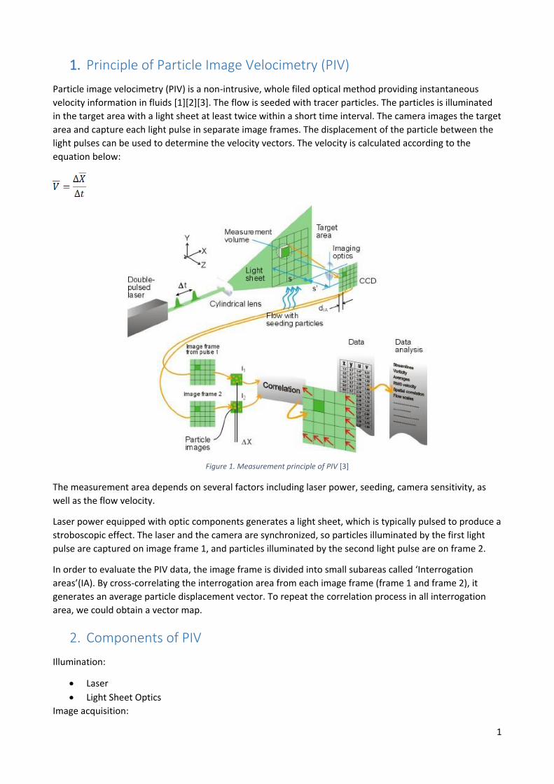
1. Principle of Particle Image Velocimetry (PIV)
Particle image velocimetry (PIV) is a non-intrusive, whole filed optical method providing instantaneous
velocity information in fluids [1][2][3]. The flow is seeded with tracer particles. The particles is illuminated
in the target area with a light sheet at least twice within a short time interval. The camera images the target
area and capture each light pulse in separate image frames. The displacement of the particle between the
light pulses can be used to determine the velocity vectors. The velocity is calculated according to the
equation below:
Figure 1. Measurement principle of PIV [3]
The measurement area depends on several factors including laser power, seeding, camera sensitivity, as
well as the flow velocity.
Laser power equipped with optic components generates a light sheet, which is typically pulsed to produce a
stroboscopic effect. The laser and the camera are synchronized, so particles illuminated by the first light
pulse are captured on image frame 1, and particles illuminated by the second light pulse are on frame 2.
In order to evaluate the PIV data, the image frame is divided into small subareas called ‘Interrogation
areas’(IA). By cross-correlating the interrogation area from each image frame (frame 1 and frame 2), it
generates an average particle displacement vector. To repeat the correlation process in all interrogation
area, we could obtain a vector map.
2. Components of PIV
Illumination:
Laser
Light Sheet Optics
Image acquisition:
2
Camera
Lenses & Filters
Data acquisition/ processing:
Synchronization
Software: DynamicStudio
Seed generation:
Seed generator
Seeding material
Accessories
3D PIV calibration tools 200*200 mm and 450*450 mm
Scheimpflug Camera Mounts
Traverse Systems and controller
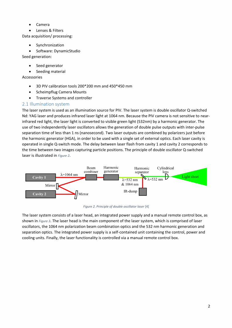
2.1 Illumination system The laser system is used as an illumination source for PIV. The laser system is double oscillator Q-switched
Nd: YAG laser and produces infrared laser light at 1064 nm. Because the PIV camera is not sensitive to near-
infrared red light, the laser light is converted to visible green light (532nm) by a harmonic generator. The
use of two independently laser oscillators allows the generation of double pulse outputs with inter-pulse
separation time of less than 1 ns (nanosecond). Two laser outputs are combined by polarizers just before
the harmonic generator (HGA), in order to be used with a single set of external optics. Each laser cavity is
operated in single Q-switch mode. The delay between laser flash from cavity 1 and cavity 2 corresponds to
the time between two images capturing particle positions. The principle of double oscillator Q-switched
laser is illustrated in Figure 2.
Figure 2. Principle of double oscillator laser [4]
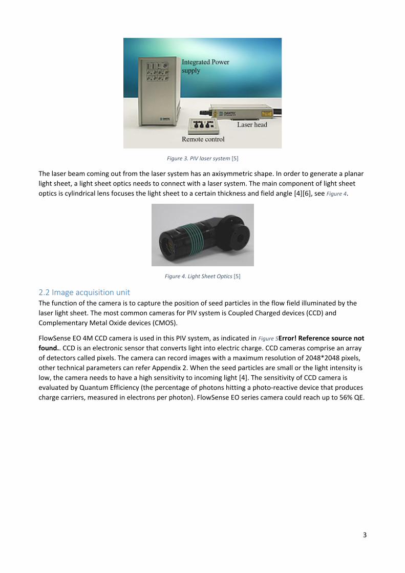
The laser system consists of a laser head, an integrated power supply and a manual remote control box, as
shown in Figure 3. The laser head is the main component of the laser system, which is comprised of laser
oscillators, the 1064 nm polarization beam combination optics and the 532 nm harmonic generation and
separation optics. The integrated power supply is a self-contained unit containing the control, power and
cooling units. Finally, the laser functionality is controlled via a manual remote control box.
3
Figure 3. PIV laser system [5]
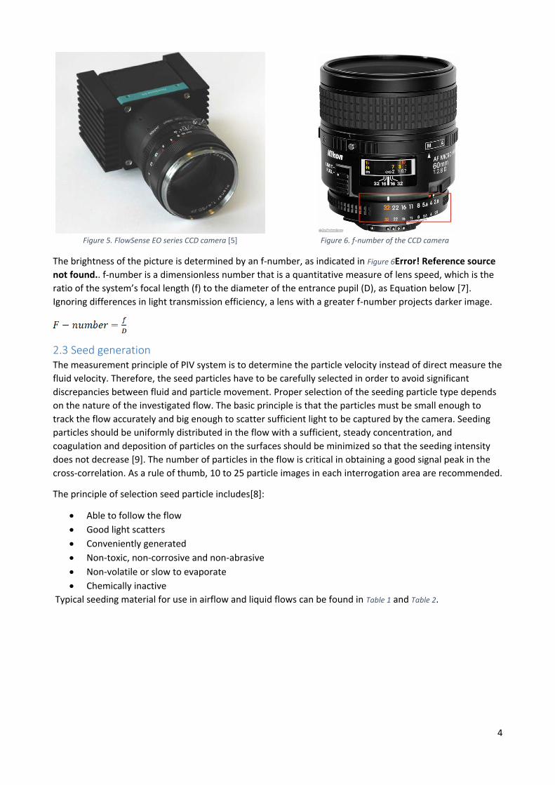
The laser beam coming out from the laser system has an axisymmetric shape. In order to generate a planar
light sheet, a light sheet optics needs to connect with a laser system. The main component of light sheet
optics is cylindrical lens focuses the light sheet to a certain thickness and field angle [4][6], see Figure 4.
Figure 4. Light Sheet Optics [5]
2.2 Image acquisition unit The function of the camera is to capture the position of seed particles in the flow field illuminated by the
laser light sheet. The most common cameras for PIV system is Coupled Charged devices (CCD) and
Complementary Metal Oxide devices (CMOS).
FlowSense EO 4M CCD camera is used in this PIV system, as indicated in Figure 5Error! Reference source not
found.. CCD is an electronic sensor that converts light into electric charge. CCD cameras comprise an array
of detectors called pixels. The camera can record images with a maximum resolution of 2048*2048 pixels,
other technical parameters can refer Appendix 2. When the seed particles are small or the light intensity is
low, the camera needs to have a high sensitivity to incoming light [4]. The sensitivity of CCD camera is
evaluated by Quantum Efficiency (the percentage of photons hitting a photo-reactive device that produces
charge carriers, measured in electrons per photon). FlowSense EO series camera could reach up to 56% QE.
4
Figure 5. FlowSense EO series CCD camera [5] Figure 6. f-number of the CCD camera
The brightness of the picture is determined by an f-number, as indicated in Figure 6Error! Reference source
not found.. f-number is a dimensionless number that is a quantitative measure of lens speed, which is the
ratio of the system’s focal length (f) to the diameter of the entrance pupil (D), as Equation below [7].
Ignoring differences in light transmission efficiency, a lens with a greater f-number projects darker image.
2.3 Seed generation The measurement principle of PIV system is to determine the particle velocity instead of direct measure the
fluid velocity. Therefore, the seed particles have to be carefully selected in order to avoid significant
discrepancies between fluid and particle movement. Proper selection of the seeding particle type depends
on the nature of the investigated flow. The basic principle is that the particles must be small enough to
track the flow accurately and big enough to scatter sufficient light to be captured by the camera. Seeding
particles should be uniformly distributed in the flow with a sufficient, steady concentration, and
coagulation and deposition of particles on the surfaces should be minimized so that the seeding intensity
does not decrease [9]. The number of particles in the flow is critical in obtaining a good signal peak in the
cross-correlation. As a rule of thumb, 10 to 25 particle images in each interrogation area are recommended.
The principle of selection seed particle includes[8]:
Able to follow the flow
Good light scatters
Conveniently generated
Non-toxic, non-corrosive and non-abrasive
Non-volatile or slow to evaporate
Chemically inactive
Typical seeding material for use in airflow and liquid flows can be found in Table 1 and Table 2.

5
Table 1. Typical seeding materials for use in airflow [2]
Material Particle diameter (μm)
Comments
Al2O3 < 8 Generated by fluidization (Useful for seeding flames on account of a high melting point)
Glycerine 0.1 - 5 Generated by atomization
Silicone oil 1 - 3 Generated by atomization (very satisfactory results)
SiO2 particles 1 - 5 (Spherical particles with a very narrow size distribution and better light scatter than TiO2)
TiO2 power from submicrometer to micrometer
(Good light scatter and stable in flames up to 2500 oC but very wide size distribution and lumped particle shapes)
Water 1 - 2 Generated by atomization (Evaporation is avoided by the addition of evaporation-inhibitor)
MgO Generated by the combustion of magnesium powder (Gives a dirty unsteady supply of seeding)
Table 2. Typical seeding materials for use in liquid flows [2]
Material Particle diameter (μm)
Comments
Aluminum powder < 10 Preserves polarization by scattering
Bubbles 5 to 500 Can only be used when the two-phase flow is acceptable. The bubbles must be in the spherical Re-Eo regime and the terminal rising velocity must be negligible to the fluid velocity
Glass spheres 10 to 150
Latex beads 0.5 to 90 Delivered with narrow size distribution but expensive
Milk 0.3 to 3 Cheap and efficient but not popular
Pine pollen 30 to 50 Excellent marker with regard to relative particle density (Egg-shaped and swell somewhat after some time in water
In the indoor environment measurement, PIV is mainly used to investigate indoor airflow. Haze machine
(Stairville Hz-200 Compact Hazer DMX) is used in the PIV system to generate haze by evaporation and
condensation of water-based haze liquid (Stairville PHF Pro Haze Fluid), see Figure 7. The haze is non-irritant
and non-flammable. The mean particle size is around 1-5 µm and the haze's durability can be controlled
through the timer remote control. The limitation of the haze machine is that the generation tends to be
unsteady and discontinuous due to the limit of heating capability.

6
Figure 7. Fog generator and seeding material [9]
2.4 Data acquisition/processing DynamicStudio is the software platform used to process PIV data measured from different flows. It a multi-
function package, which contains tools for configuration, acquisition, analysis, post-processing of acquired
data [10].
Figure 8. DynamicStudio [5]
On the other hand, the software needs to cooperate with a synchronization unit, as indicated in Figure 9. The
camera and the laser cavities need be synchronous to capture PIV images with a specified time difference.
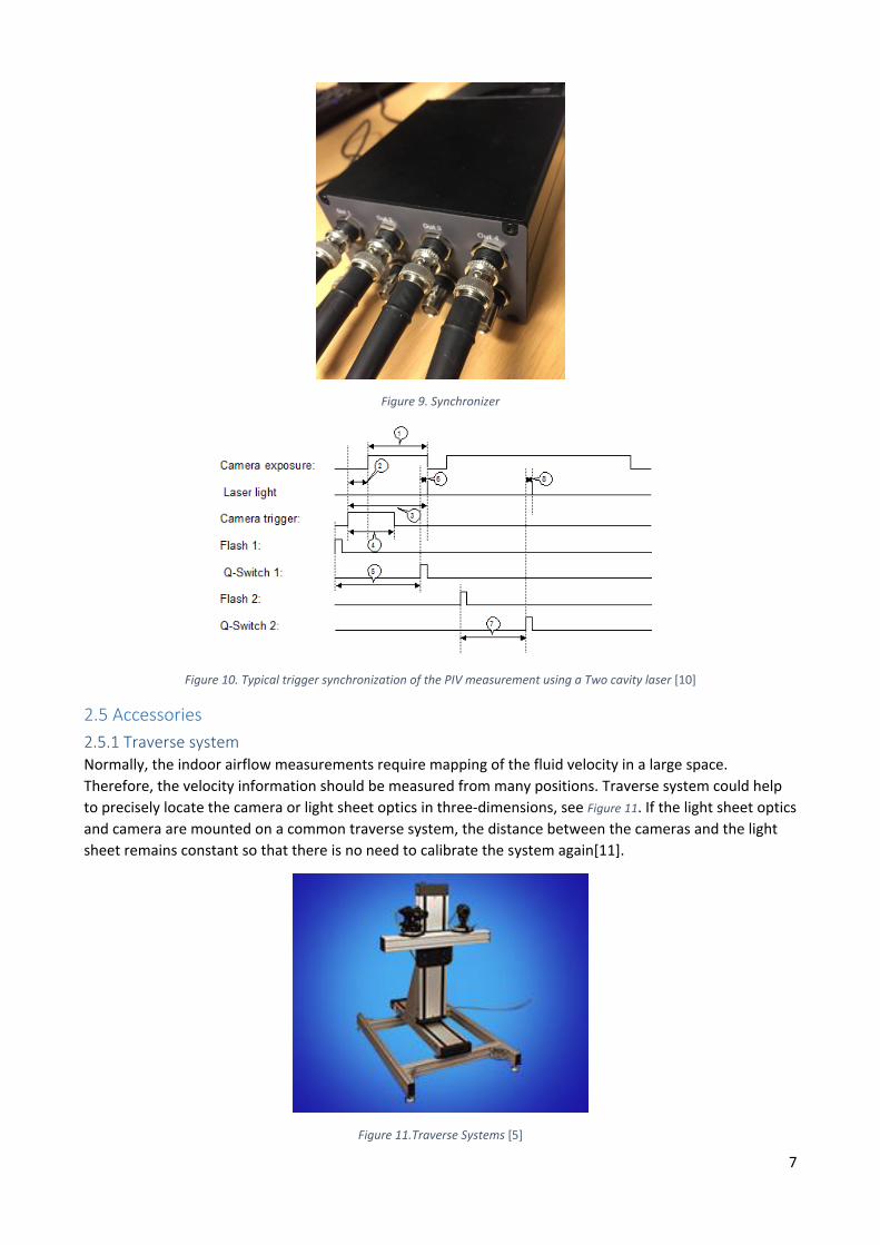
7
Figure 9. Synchronizer
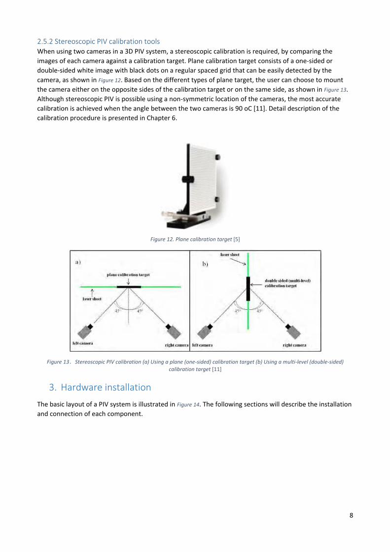
Figure 10. Typical trigger synchronization of the PIV measurement using a Two cavity laser [10]
2.5 Accessories
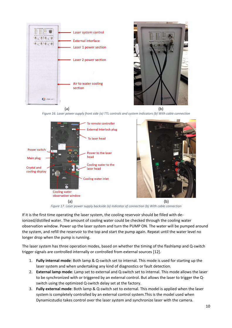
2.5.1 Traverse system Normally, the indoor airflow measurements require mapping of the fluid velocity in a large space.
Therefore, the velocity information should be measured from many positions. Traverse system could help
to precisely locate the camera or light sheet optics in three-dimensions, see Figure 11. If the light sheet optics
and camera are mounted on a common traverse system, the distance between the cameras and the light
sheet remains constant so that there is no need to calibrate the system again[11].
Figure 11.Traverse Systems [5]
8
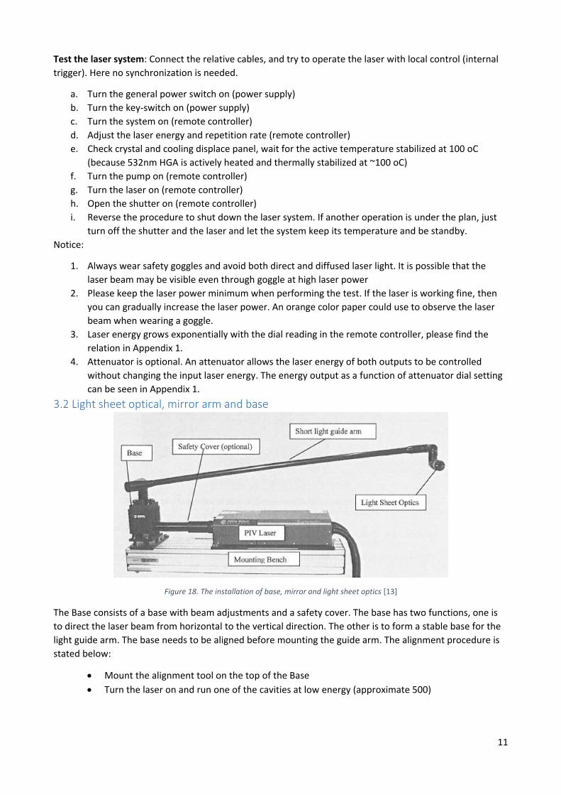
2.5.2 Stereoscopic PIV calibration tools When using two cameras in a 3D PIV system, a stereoscopic calibration is required, by comparing the
images of each camera against a calibration target. Plane calibration target consists of a one-sided or
double-sided white image with black dots on a regular spaced grid that can be easily detected by the
camera, as shown in Figure 12. Based on the different types of plane target, the user can choose to mount
the camera either on the opposite sides of the calibration target or on the same side, as shown in Figure 13.
Although stereoscopic PIV is possible using a non-symmetric location of the cameras, the most accurate
calibration is achieved when the angle between the two cameras is 90 oC [11]. Detail description of the
calibration procedure is presented in Chapter 6.
Figure 12. Plane calibration target [5]
Figure 13.Stereoscopic PIV calibration (a) Using a plane (one-sided) calibration target (b) Using a multi-level (double-sided) calibration target [11]
3. Hardware installation
The basic layout of a PIV system is illustrated in Figure 14. The following sections will describe the installation
and connection of each component.

9
Figure 14. Layout of PIV measurement
3.1 Laser system The laser system is composed of a laser head, power supply unit and laser system control, as shown in Figure
15. The laser head should be placed on a secure optical table for mounting rig and fixed down using the
mounting feet provided. The power supply unit should be located in the free space that allows the cooling
air circulation. The laser head should be installed in a place that the light sheet can pass the measurement
object.
(a) (b) (c)
Figure 15. Laser system (a) Laser head (b) Power supply (c) Remote controller
The main connection panel of the laser system is shown in Figure 16 and Figure 17.
10
(a) (b)
Figure 16. Laser power supply front side (a) TTL controls and system indicators (b) With cable connection
(a) (b)
Figure 17. Laser power supply backside (a) Indicator of connection (b) With cable connection
If it is the first time operating the laser system, the cooling reservoir should be filled with de-
ionized/distilled water. The amount of cooling water could be checked through the cooling water
observation window. Power up the laser system and turn the PUMP ON. The water will be pumped around
the system, and refill the reservoir to the top and start the pump again. Repeat until the water level no
longer drop when the pump is running.
The laser system has three operation modes, based on whether the timing of the flashlamp and Q-switch
trigger signals are controlled internally or controlled from external sources [12].
1. Fully internal mode: Both lamp & Q-switch set to internal. This mode is used for starting up the
laser system and when undertaking any kind of diagnostics or fault detection.
2. External lamp mode: Lamp set to external and Q-switch set to internal. This mode allows the laser
to be synchronized with or triggered by an external control. But allows the laser to trigger the Q-
switch using the optimized Q-switch delay set at the factory.
3. Fully external mode: Both lamp & Q-switch set to external. This model is applied when the laser
system is completely controlled by an external control system.This is the model used when
Dynamicstudio takes control over the laser system and synchronize laser with the camera.
11
Test the laser system: Connect the relative cables, and try to operate the laser with local control (internal
trigger). Here no synchronization is needed.
a. Turn the general power switch on (power supply)
b. Turn the key-switch on (power supply)
c. Turn the system on (remote controller)
d. Adjust the laser energy and repetition rate (remote controller)
e. Check crystal and cooling displace panel, wait for the active temperature stabilized at 100 oC
(because 532nm HGA is actively heated and thermally stabilized at ~100 oC)
f. Turn the pump on (remote controller)
g. Turn the laser on (remote controller)
h. Open the shutter on (remote controller)
i. Reverse the procedure to shut down the laser system. If another operation is under the plan, just
turn off the shutter and the laser and let the system keep its temperature and be standby.
Notice:
1. Always wear safety goggles and avoid both direct and diffused laser light. It is possible that the
laser beam may be visible even through goggle at high laser power
2. Please keep the laser power minimum when performing the test. If the laser is working fine, then
you can gradually increase the laser power. An orange color paper could use to observe the laser
beam when wearing a goggle.
3. Laser energy grows exponentially with the dial reading in the remote controller, please find the
relation in Appendix 1.
4. Attenuator is optional. An attenuator allows the laser energy of both outputs to be controlled
without changing the input laser energy. The energy output as a function of attenuator dial setting
can be seen in Appendix 1.
3.2 Light sheet optical, mirror arm and base
Figure 18. The installation of base, mirror and light sheet optics [13]
The Base consists of a base with beam adjustments and a safety cover. The base has two functions, one is
to direct the laser beam from horizontal to the vertical direction. The other is to form a stable base for the
light guide arm. The base needs to be aligned before mounting the guide arm. The alignment procedure is
stated below:
Mount the alignment tool on the top of the Base
Turn the laser on and run one of the cavities at low energy (approximate 500)

12
Check the laser beam whether on the center of the small knob of the alignment tool. If not, the
four top screws can be loosened and the top plate with the cover can be moved until the beam
is centered
Lock the 4 screws in this position and remove the alignment tool.
Figure 19. Alignment of the Base [13]
After the alignment of the Base, the light guide arm can be mounted. The light guides arm allows a flexible
delivery of the laser beam. The light guides are articulated arms with 5 or 6 mirrors, and the mirrors are
pre-aligned to keep the laser beam centered in the aperture regardless of movement of the light guide.
The light sheet optics converts the pulsing beam from an ND: YAG laser into a pulsing laser light sheet. The
optics produce a light-sheet with fixed or adjustable thickness, enabling the user to generate light-sheets
for almost any flow illumination application.
3.3 CCD Camera
Figure 20. CCD camera and its connections
The camera has three connections: power, synchronization signal, and data output. The synchronization
sign connects to timer box, see Figure 20. The data output connects to PC, and power connects to the power
supply. After the camera is connected, power is on and the DynamicStudio will detect the camera
automatically if it is open.
After DynamicStudio detects the camera, remove the cap of the lens, operate the camera with Free Run
mode. Detail information regarding how to operate the camera is in Section 4.2. It is important to notice
that always protect the camera from the direct illumination of laser light. This is the most common type of
damage.

13
3.4 Timer box/Synchronizer The timer box works together with DynamicStudio to synchronize the camera, the laser and the flow to be
measured. The connection of the timer is shown in Figure 21 and Figure 22.
Figure 21. Connection of the timer with laser and camera [10]
Figure 22. Synchronizer output channels connected with laser power and camera
If two cameras are used for 3D measurement, use a three-way connection to connect the two cameras and
the time box, as shown in Figure 23Error! Reference source not found..
Figure 23. Three way valve
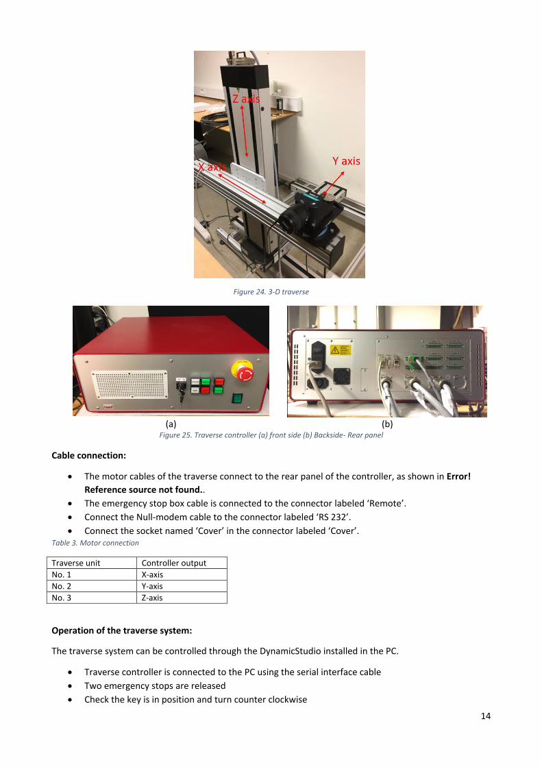
3.5 3-D traverse The system contains X, Y, Z traverse, a traverse controller and an emergency stop box.
14
Figure 24. 3-D traverse
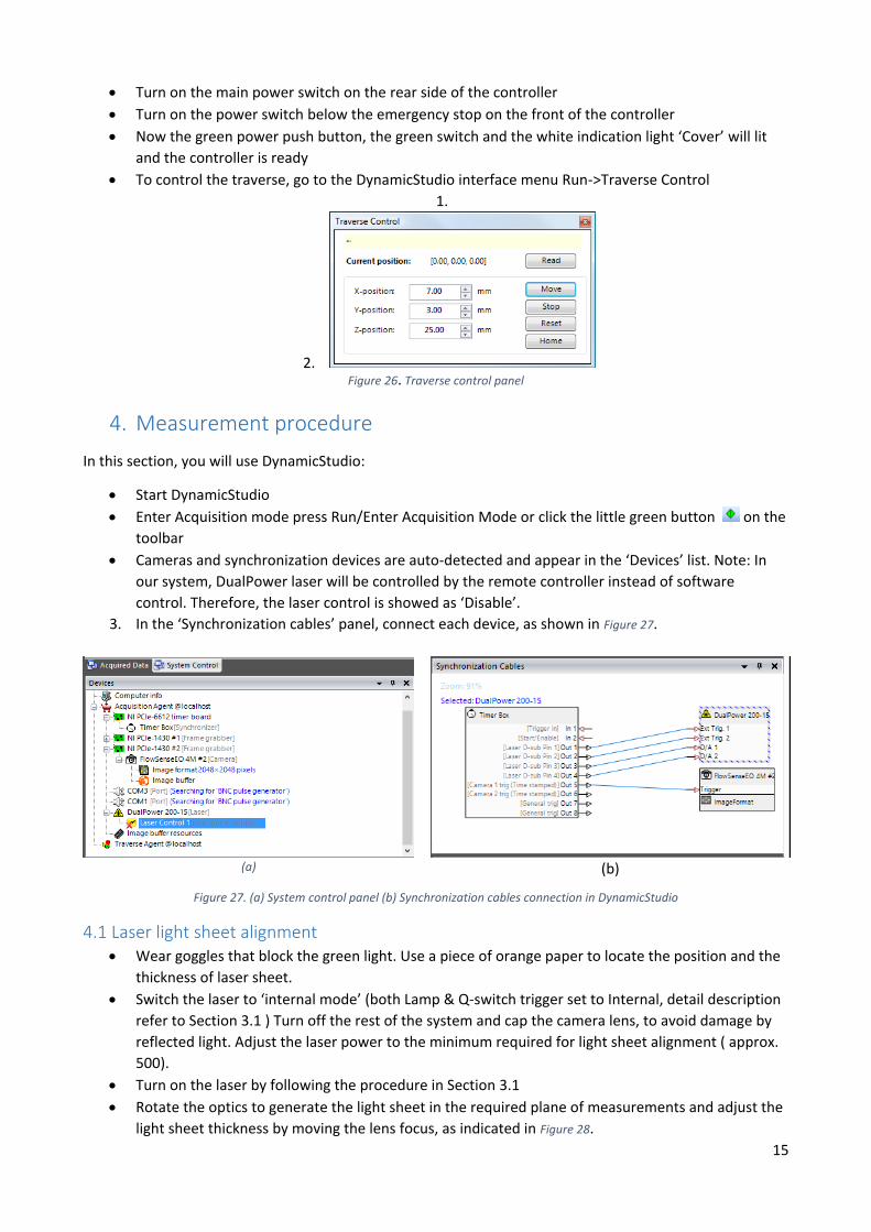
(a) (b)
Figure 25. Traverse controller (a) front side (b) Backside- Rear panel
Cable connection:
The motor cables of the traverse connect to the rear panel of the controller, as shown in Error!
Reference source not found..
The emergency stop box cable is connected to the connector labeled ‘Remote’.
Connect the Null-modem cable to the connector labeled ‘RS 232’.
Connect the socket named ‘Cover’ in the connector labeled ‘Cover’. Table 3. Motor connection
Traverse unit Controller output
No. 1 X-axis
No. 2 Y-axis
No. 3 Z-axis
Operation of the traverse system:
The traverse system can be controlled through the DynamicStudio installed in the PC.
Traverse controller is connected to the PC using the serial interface cable
Two emergency stops are released
Check the key is in position and turn counter clockwise
15
Turn on the main power switch on the rear side of the controller
Turn on the power switch below the emergency stop on the front of the controller
Now the green power push button, the green switch and the white indication light ‘Cover’ will lit
and the controller is ready
To control the traverse, go to the DynamicStudio interface menu Run->Traverse Control
1.
2. Figure 26. Traverse control panel
4. Measurement procedure
In this section, you will use DynamicStudio:
Start DynamicStudio
Enter Acquisition mode press Run/Enter Acquisition Mode or click the little green button on the
toolbar
Cameras and synchronization devices are auto-detected and appear in the ‘Devices’ list. Note: In
our system, DualPower laser will be controlled by the remote controller instead of software
control. Therefore, the laser control is showed as ‘Disable’.
3. In the ‘Synchronization cables’ panel, connect each device, as shown in Figure 27.
(a) (b)
Figure 27. (a) System control panel (b) Synchronization cables connection in DynamicStudio
4.1 Laser light sheet alignment Wear goggles that block the green light. Use a piece of orange paper to locate the position and the
thickness of laser sheet.
Switch the laser to ‘internal mode’ (both Lamp & Q-switch trigger set to Internal, detail description
refer to Section 3.1 ) Turn off the rest of the system and cap the camera lens, to avoid damage by
reflected light. Adjust the laser power to the minimum required for light sheet alignment ( approx.
500).
Turn on the laser by following the procedure in Section 3.1
Rotate the optics to generate the light sheet in the required plane of measurements and adjust the
light sheet thickness by moving the lens focus, as indicated in Figure 28.

16
Select a suitable height of light sheet based on the distance between sheet optics and the field of
view and the size of the field of view.
Minimize surface reflection light and check that none hits the camera lens.
Switch the laser off and set back the laser to ‘External mode’.
Figure 28. Images of slightly misaligned light sheets [2]
Note: The main velocity component of flow should be parallel to the light sheet, in order to minimize
systematic errors and out-of-plane loss of particles.
4.2 Camera setup and calibration Camera alignment:
Switch off the laser or keep the laser in internal trigger mode
Put the plane target in the measurement area.
Enter the acquisition mode and set up the acquisition parameters in ‘System control’ panel. ‘Single
frame mode’ should be selected, as shown in Figure 29.
Long exposure time is required for the camera to capture enough illumination, since no laser
illumination. The exposure time can be set in the Devices Properties panel, corresponding to the
selected camera. A long exposure time, such as 10000 µs or longer is suggested.
Click Free Run in System Control panel to start acquiring image
Refine the position or the attitude of the camera as well as its focus
You can use ‘Online Focus Assist’ to tune the focus of the camera (right click the ‘Image Format’
device and select ‘Add Online Analysis’, then select ‘Online Focus Assist’, detail refer to [10])
Figure 29. Acquisition setup in System Control Panel
There are three different ways of acquiring images with DynamicStudio, corresponding to the three
topmost buttons in the right-hand side of the system control window:
17
Free Run: In free run, the camera is running freely and not synchronized with other hardware
devices. The laser is not activated in this mode.
Preview: In preview mode, all devices are synchronized, the laser is flashing and the camera is
triggered to acquire images at the rate specified in the System Control panel. It will not stop
acquiring images until you press Stop.
Acquire: Acquire does exactly the same as Preview with the one exception that it stops when the
requested number of images have been acquired.
Calibration of the camera:
The purpose of capture the calibration image is to provide dimensional information to the measurement
field. The calibration procedure is based on following steps:
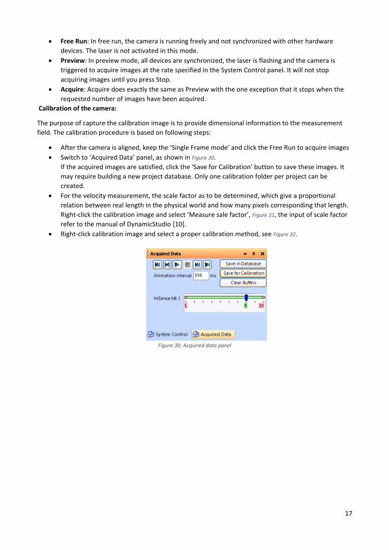
After the camera is aligned, keep the ‘Single Frame mode’ and click the Free Run to acquire images
Switch to ‘Acquired Data’ panel, as shown in Figure 30.
If the acquired images are satisfied, click the ‘Save for Calibration’ button to save these images. It
may require building a new project database. Only one calibration folder per project can be
created.
For the velocity measurement, the scale factor as to be determined, which give a proportional
relation between real length in the physical world and how many pixels corresponding that length.
Right-click the calibration image and select ‘Measure sale factor’, Figure 31, the input of scale factor
refer to the manual of DynamicStudio [10].
Right-click calibration image and select a proper calibration method, see Figure 32.
Figure 30. Acquired data panel

18
Figure 31. Measure scale factor
Figure 32. Select calibration method
4.3 Data acquisition The data acquisition procedure is similar to that of the capture of the calibration image. But the following
different steps should be awarded:
Select ‘ Double Frame mode’ in the System Control panel
Adjust the ‘Time between pulses’. The time between pulses should be long enough to determine
the displacement of the particles between two pulses, also need to be short enough to avoid
particles leaving out of the interrogation area. PIV Setup Assistant could help to calculate a suitable
value of ∆t based on provided information, see Figure 33.
Check all the connections and verify the laser is prepared for illumination (connection is correct,
the laser is pre-warmed, both flash lamp and Q-switch are set to ‘External’ trigger, the laser power
is optimized, etc.)
Specify the number of images to acquire and trigger rate

19
Camera exposure time should be reduced, due to laser will be used for illumination. Start from the
minimum exposure time 10-15 µs based on camera series.
Start the ‘Acquire mode’
Click ‘ Save in Database’ if the image quality is acceptable. The quality of image could be check by
observing the cross-correlation map immediately. Right-click the acquired image, select ‘Cross-
Correlation Map’, the cross-correlation map to each interrogation area can be observed (Figure 34).
It is better to repeat each measurement several times to achieve accuracy results (for example
repeat each measurement 5 times and use the average value)
Figure 33. PIV Setup Assistant
(a) (b)
Figure 34. Cross-correlation map [10]

20
4.4 Data Processing After saving the acquired images, select ‘Database’ from ‘View’ on the top of DynamicStudio.
Select the images would like to be processed, right-click one of them, select ‘Analyze’. Then choose
suitable analysis method in the ‘Select Analysis Method’ panel, see Figure 35. Detail description
regarding analysis method refers to DynamicStudio manual [10].
4.
5.
(a) (b) Figure 35. Data processing (a) Entrance of image analyze mode (b) Window of select Analysis Method
The correlation signal is strongly affected by the variation in image intensity. The non-uniform
illumination of particle image intensity, due to light-sheet non-uniformities or pulse-to-pulse
variation, or irregular particle shape, out-of-plane motion, etc., create noise in the correlation
signal [1]. Therefore, pre-processing of particle image is often very necessary, Select the proper
image process method, in the image processing library. Several commonly used functions are
described below:
o ‘ROI Extract’ is to extract interest region from the original acquired image. Therefore, time
to processing the images will be shorter.
o ‘Image masking’ is another method to remove areas of no interest from an acquired image.
o ‘Background subtraction’ from the PIV recordings reduces the background noise. The
background image can either be recorded in the absence of seeding, or through ‘Image
mean’ to calculate the average intensity of corresponding pixels in all the selected images.
A minimum selection of two images is required. Then the background image could be
removed using ‘Image Arithmetic’, as shown in Figure 36.
21
Figure 36. Background subtraction
After pre-processing image, the image evaluation method need be applied to convert pairs of
particle images into velocity field. Select the calibration results, and then select the images to be
analyzed by right click the image and select ‘Analyze’ option. Select the proper image evaluation
method, in the PIV Signal library. Note: Read and study the instruction of each process algorithm
carefully. The most suitable analysis method may be different depending on the measurement. It is
recommended to try different PIV process method or different parameters to compare the results
and understand the influence of the algorithm on the results.
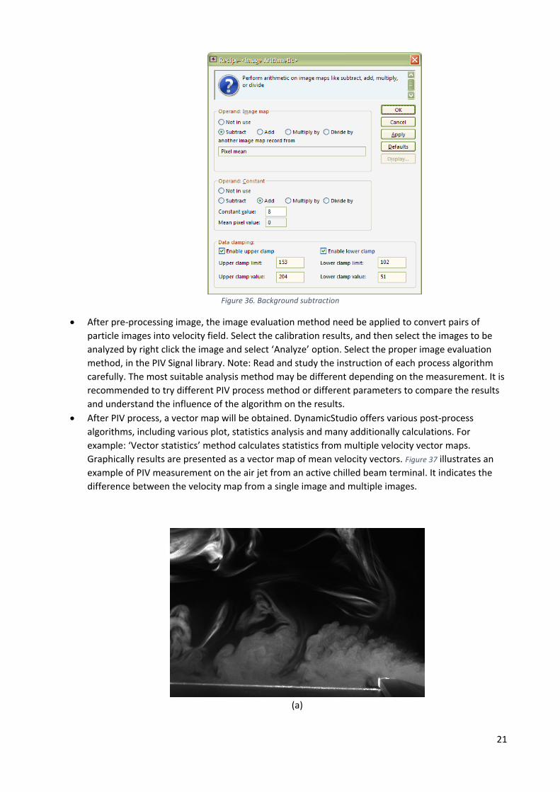
After PIV process, a vector map will be obtained. DynamicStudio offers various post-process
algorithms, including various plot, statistics analysis and many additionally calculations. For
example: ‘Vector statistics’ method calculates statistics from multiple velocity vector maps.
Graphically results are presented as a vector map of mean velocity vectors. Figure 37 illustrates an
example of PIV measurement on the air jet from an active chilled beam terminal. It indicates the
difference between the velocity map from a single image and multiple images.
(a)

22
(b)
(c)
Figure 37. PIV measurement of air jet from an active chilled beam terminal (a) Acquired particle image (b) Instantaneous velocity vector field (single image) (c) Averaged velocity vector field (200 images) [14]
5. Image evaluation method for PIV
The statistical PIV evaluation will be used to calculate the velocity field from pairs of particle images.
5.1 Cross-correlation
Figure 38. The cross-correlation method [1]
Two sequential images describing the spatial positions of particles are recorded at time t and time t+∆t. The
velocity field is not directly calculated on the whole images but on the small subareas called interrogation
areas (IA). Within each interrogation area, an average displacement of particles is determined from one
sample to its pair in the second image. The displacement is directly related to the flow and the time
23
between two images and it can be calculated by the statistical algorithm of cross-correlation. High cross-
correlation values are observed where many particles match up with their corresponding partners.
Therefore, the position of the peak corresponds to the average particles displacement in the IA.
The direct calculation of cross-correlation is very time-consuming and expensive to apply due to a large
number of particles to be analyzed. Fast Fourier Transform (FFT) is a more efficient way to calculate cross-
correlation which reduces the computation from O[N4] operations to O[N2 log2 N] operations [1] [4]. The
most common FFT implementation requires the input data to have a base-2 dimension (i.e. 32 × 32 pixel or
64 × 64 pixel samples). FFT also assumes the sampled regions to be periodic in space. The consequence of
the mathematical simplification of FFT is a dramatical increase of the noise along the edges of the IA. This is
compensated by applying window or filter functions to the PIV calculations.
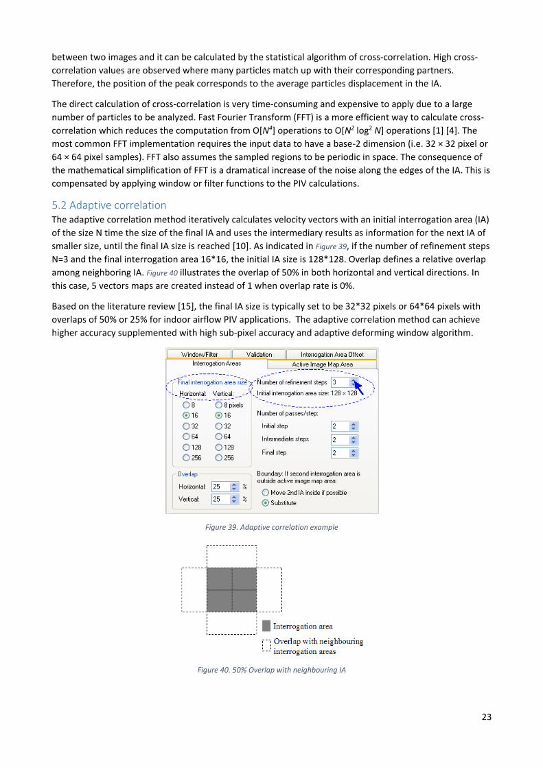
5.2 Adaptive correlation The adaptive correlation method iteratively calculates velocity vectors with an initial interrogation area (IA)
of the size N time the size of the final IA and uses the intermediary results as information for the next IA of
smaller size, until the final IA size is reached [10]. As indicated in Figure 39, if the number of refinement steps
N=3 and the final interrogation area 16*16, the initial IA size is 128*128. Overlap defines a relative overlap
among neighboring IA. Figure 40 illustrates the overlap of 50% in both horizontal and vertical directions. In
this case, 5 vectors maps are created instead of 1 when overlap rate is 0%.
Based on the literature review [15], the final IA size is typically set to be 32*32 pixels or 64*64 pixels with
overlaps of 50% or 25% for indoor airflow PIV applications. The adaptive correlation method can achieve
higher accuracy supplemented with high sub-pixel accuracy and adaptive deforming window algorithm.
Figure 39. Adaptive correlation example
Figure 40. 50% Overlap with neighbouring IA
24
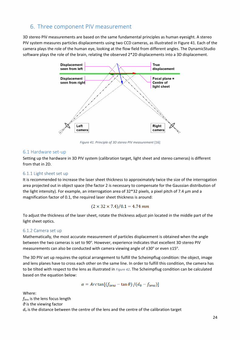
6. Three component PIV measurement
3D stereo PIV measurements are based on the same fundamental principles as human eyesight. A stereo
PIV system measures particles displacements using two CCD cameras, as illustrated in Figure 41. Each of the
camera plays the role of the human eye, looking at the flow field from different angles. The DynamicStudio
software plays the role of the brain, relating the observed 2*2D displacements into a 3D displacement.
Figure 41. Principle of 3D stereo PIV measurement [16]
6.1 Hardware set-up Setting up the hardware in 3D PIV system (calibration target, light sheet and stereo cameras) is different
from that in 2D.
6.1.1 Light sheet set up It is recommended to increase the laser sheet thickness to approximately twice the size of the interrogation
area projected out in object space (the factor 2 is necessary to compensate for the Gaussian distribution of
the light intensity). For example, an interrogation area of 32*32 pixels, a pixel pitch of 7.4 µm and a
magnification factor of 0.1, the required laser sheet thickness is around:
To adjust the thickness of the laser sheet, rotate the thickness adjust pin located in the middle part of the
light sheet optics.
6.1.2 Camera set up Mathematically, the most accurate measurement of particles displacement is obtained when the angle
between the two cameras is set to 90o. However, experience indicates that excellent 3D stereo PIV
measurements can also be conducted with camera viewing angle of ±30o or even ±15o.
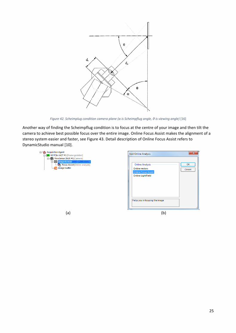
The 3D PIV set up requires the optical arrangement to fulfill the Scheimpflug condition: the object, image
and lens planes have to cross each other on the same line. In order to fulfill this condition, the camera has
to be tilted with respect to the lens as illustrated in Figure 42. The Scheimpflug condition can be calculated
based on the equation below:
Where: flens is the lens focus length θ is the viewing factor do is the distance between the centre of the lens and the centre of the calibration target
25
Figure 42. Scheimplug condition camera plane (󠄀α is Scheimpflug angle, θ is viewing angle) [16]
Another way of finding the Scheimpflug condition is to focus at the centre of your image and then tilt the
camera to achieve best possible focus over the entire image. Online Focus Assist makes the alignment of a
stereo system easier and faster, see Figure 43. Detail description of Online Focus Assist refers to
DynamicStudio manual [10].
(a) (b)

26
(c)
Figure 43. Using Online Focus Assist to set up a stereo PIV system [10]
6.1.3 Calibration target Before conducting calibration, it is necessary to define how large the flow field of interest is and select
appropriate calibration target. The standard calibration target is 200 mm*200 mm. If the flow field area is
larger, a larger calibration target is required. If the flow field area is smaller than 50 mm*50 mm, the
number of dots will be too small. A target with a smaller dot pitch is needed. In order to achieve best
calibration, each calibration image has to have at least 100 visible dots.
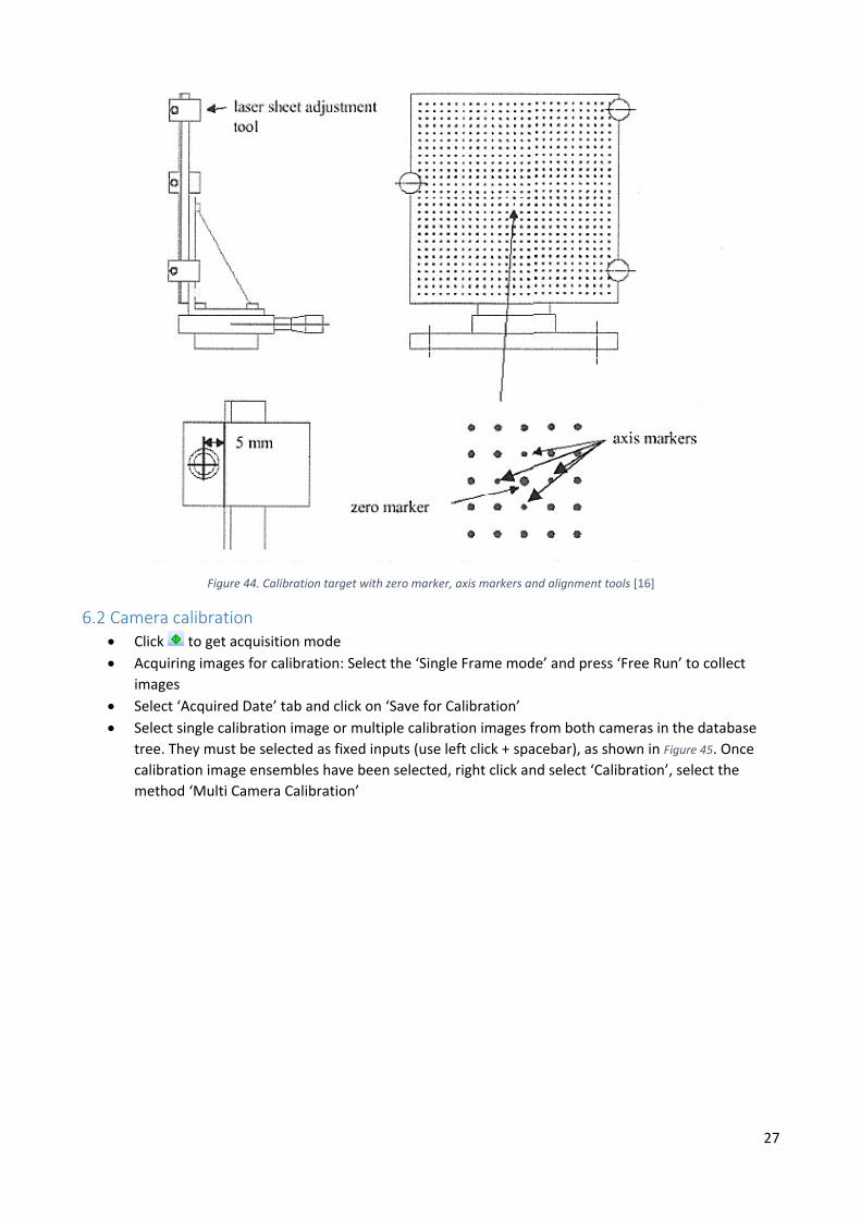
Align the calibration target with the light sheet and install it in the centre of the flow field. Alignment tools
could be applied to align the light sheet with the calibration target. The tool includes three small units with
hole allowing laser light to pass through. The center of the holes are exactly 5 mm from the front of the
calibration target, so during alignment the target should be traversed 5 mm away from the position where
calibration images are acquired.
27
Figure 44. Calibration target with zero marker, axis markers and alignment tools [16]
6.2 Camera calibration Click to get acquisition mode
Acquiring images for calibration: Select the ‘Single Frame mode’ and press ‘Free Run’ to collect
images
Select ‘Acquired Date’ tab and click on ‘Save for Calibration’
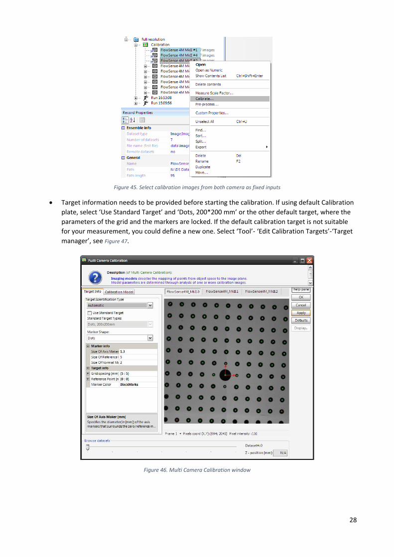
Select single calibration image or multiple calibration images from both cameras in the database
tree. They must be selected as fixed inputs (use left click + spacebar), as shown in Figure 45. Once
calibration image ensembles have been selected, right click and select ‘Calibration’, select the
method ‘Multi Camera Calibration’
28
Figure 45. Select calibration images from both camera as fixed inputs
Target information needs to be provided before starting the calibration. If using default Calibration
plate, select ‘Use Standard Target’ and ‘Dots, 200*200 mm’ or the other default target, where the
parameters of the grid and the markers are locked. If the default calibration target is not suitable
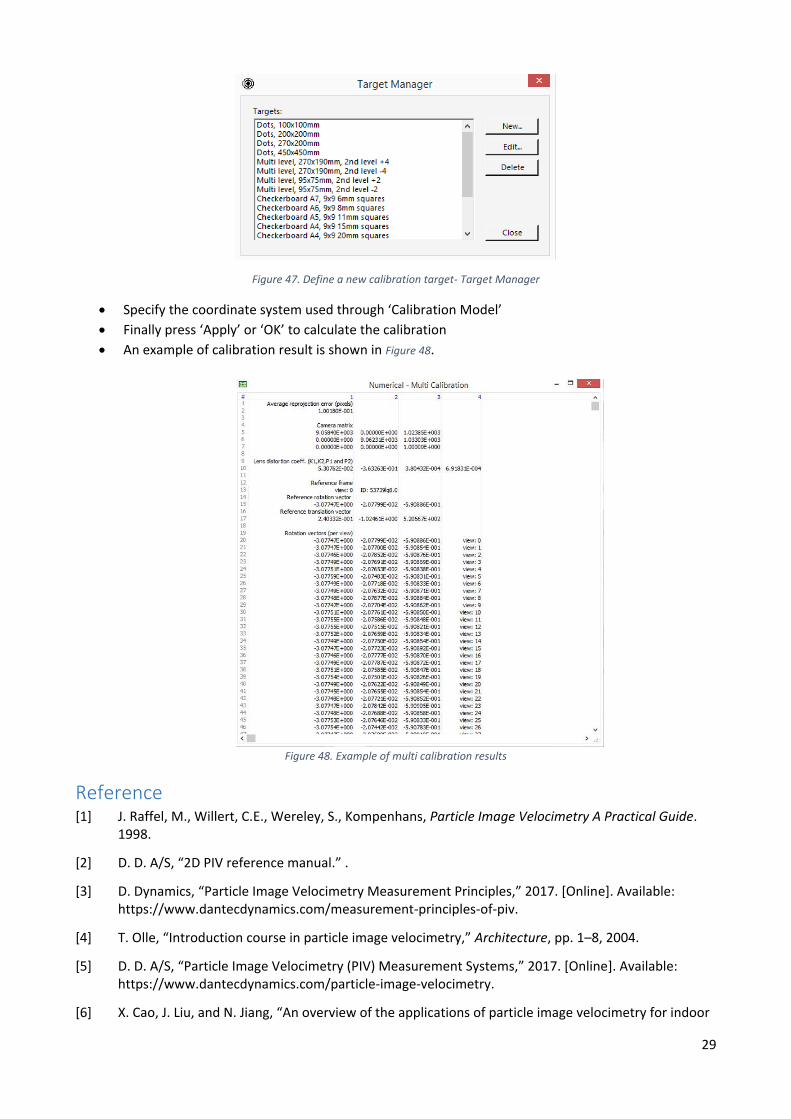
for your measurement, you could define a new one. Select ‘Tool’- ‘Edit Calibration Targets’-‘Target
manager’, see Figure 47.
Figure 46. Multi Camera Calibration window
29
Figure 47. Define a new calibration target- Target Manager
Specify the coordinate system used through ‘Calibration Model’
Finally press ‘Apply’ or ‘OK’ to calculate the calibration
An example of calibration result is shown in Figure 48.
Figure 48. Example of multi calibration results
Reference [1] J. Raffel, M., Willert, C.E., Wereley, S., Kompenhans, Particle Image Velocimetry A Practical Guide.
1998.
[2] D. D. A/S, “2D PIV reference manual.” .
[3] D. Dynamics, “Particle Image Velocimetry Measurement Principles,” 2017. [Online]. Available: https://www.dantecdynamics.com/measurement-principles-of-piv.
[4] T. Olle, “Introduction course in particle image velocimetry,” Architecture, pp. 1–8, 2004.
[5] D. D. A/S, “Particle Image Velocimetry (PIV) Measurement Systems,” 2017. [Online]. Available: https://www.dantecdynamics.com/particle-image-velocimetry.
[6] X. Cao, J. Liu, and N. Jiang, “An overview of the applications of particle image velocimetry for indoor

30
airflow field measurement,” Lect. Notes Electr. Eng., vol. 263 LNEE, no. VOL. 3, pp. 223–231, 2014.
[7] F. Wikipedia, “f-number - Wikipedia.” [Online]. Available: https://en.wikipedia.org/wiki/F-number. [Accessed: 14-May-2017].
[8] A. M. and J. H. W. R. Durst, Principles and practice of laser-Doppler anemometry, 2nd ed. Academic Press Inc, 1981.
[9] “Stairville HZ-200 COMPACT HAZER DM BUNDLE - Skylark,” 2018. .
[10] “DynamicStudio Manual.pdf.” .
[11] S. A. Jones, Advanced Methods for Pratical Applications in Fluid Mechanics. InTech, 2012.
[12] “Laser system user manual.pdf.” .
[13] D. D. A/S, “Mirror arm and base for Pulsed lasers- Installation & User’s guide,” 2003.
[14] S. V. B. Kozlowski, “Active chilled beams - Air distribution and efficiency,” Aalborg University, 2017.
[15] X. Cao, J. Liu, N. Jiang, and Q. Chen, “Particle image velocimetry measurement of indoor airflow field : A review of the technologies and applications,” Energy Build., vol. 69, pp. 367–380, 2014.
[16] D. D. A/S, 3D Stereoscopic PIV Reference Manual.pdf. 2006.

31
Appendix 1: Laser Specifications

32
33
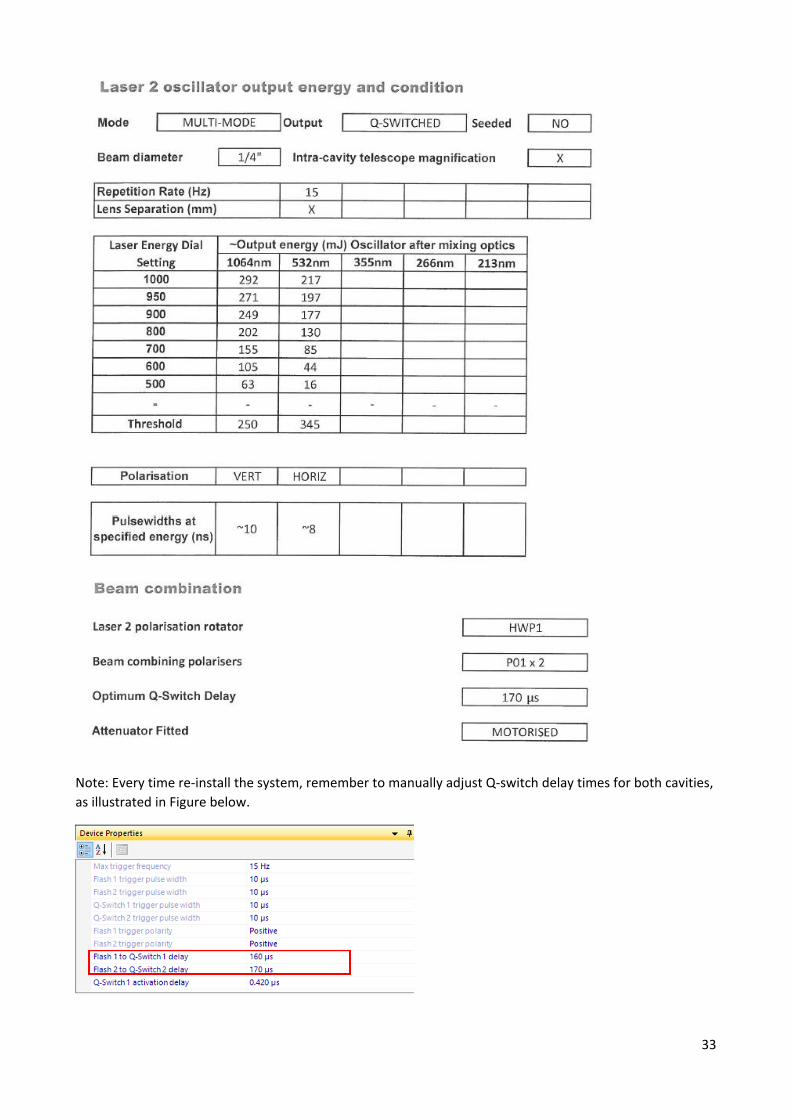
Note: Every time re-install the system, remember to manually adjust Q-switch delay times for both cavities,
as illustrated in Figure below.

34
35
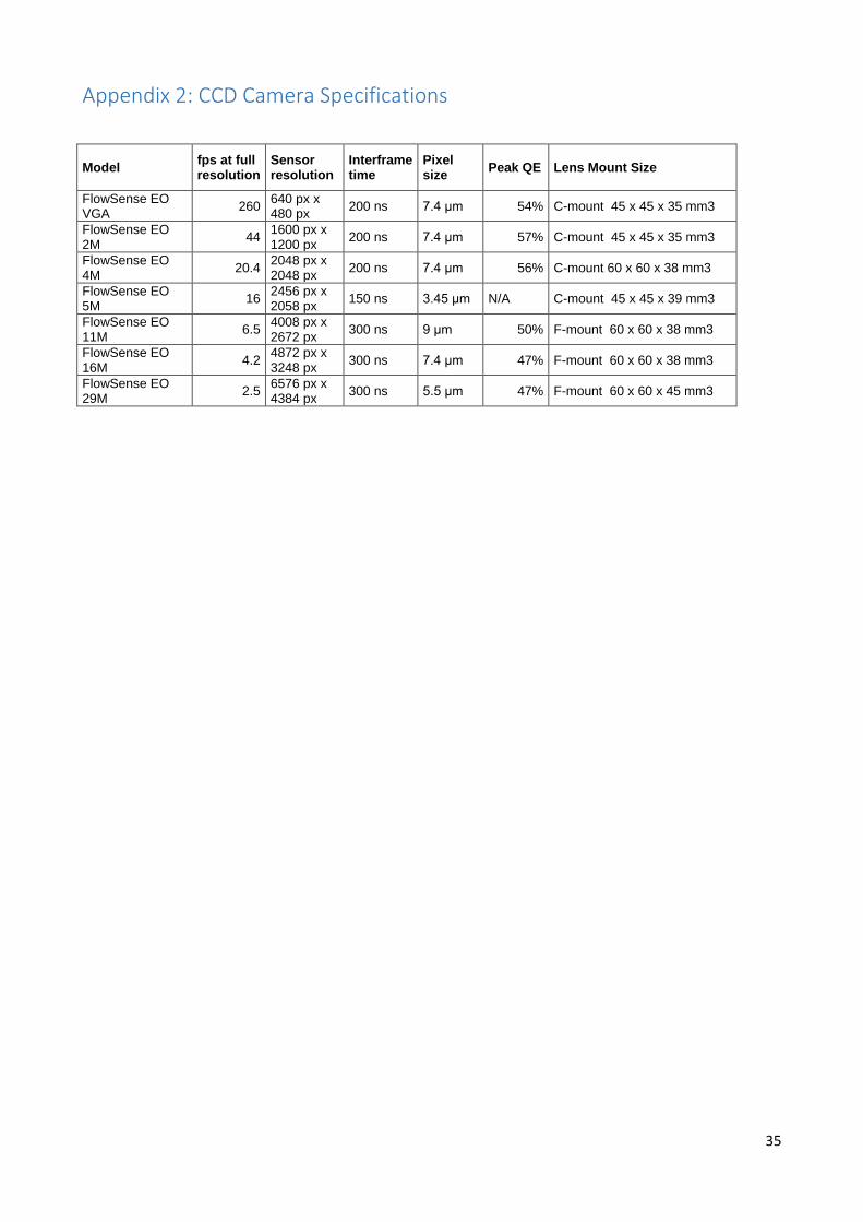
Appendix 2: CCD Camera Specifications
Model fps at full resolution
Sensor resolution
Interframe time
Pixel size
Peak QE Lens Mount Size
FlowSense EO VGA
260 640 px x 480 px
200 ns 7.4 μm 54% C-mount 45 x 45 x 35 mm3
FlowSense EO 2M
44 1600 px x 1200 px
200 ns 7.4 μm 57% C-mount 45 x 45 x 35 mm3
FlowSense EO 4M
20.4 2048 px x 2048 px
200 ns 7.4 μm 56% C-mount 60 x 60 x 38 mm3
FlowSense EO 5M
16 2456 px x 2058 px
150 ns 3.45 μm N/A C-mount 45 x 45 x 39 mm3
FlowSense EO 11M
6.5 4008 px x 2672 px
300 ns 9 μm 50% F-mount 60 x 60 x 38 mm3
FlowSense EO 16M
4.2 4872 px x 3248 px
300 ns 7.4 μm 47% F-mount 60 x 60 x 38 mm3
FlowSense EO 29M
2.5 6576 px x 4384 px
300 ns 5.5 μm 47% F-mount 60 x 60 x 45 mm3

ISSN 1901-726X DCE Technical Report No. 237