Embed Size (px)
Citation preview
Language Engineering for Information Extraction
Von der Fakultat fur Mathematik und Informatik
der Universitat Leipzig
angenommene
D I S S E R T A T I O N
zur Erlangung des akademischen Grades
DOCTOR rerum naturalium
(Dr. rer. nat.)
im Fachgebiet
Informatik
vorgelegt
von Dipl.-Inf. Martin Schierle
geboren am 03.02.1981 in Boblingen
Redwood City, den 26.12.2011
Die Annahme der Dissertation wurde empfohlen von:
1. Prof. Dr. Gerhard Heyer, Universitat Leipzig
2. Prof. Dr. Stefan Wrobel, Universitat Bonn
Die Verleihung des akademischen Grades erfolgt mit Bestehen der Verteidigung
am 07. Dezember 2011 mit dem Gesamtpradikat magna cum laude.


Hiermit erklare ich, die vorliegende Dissertation selbstandig und ohne unzulassige fremde
Hilfe angefertigt zu haben. Ich habe keine anderen als die angefuhrten Quellen und Hilfsmit-
tel benutzt und samtliche Textstellen, die wortlich oder sinngemaß aus veroffentlichten oder
unveroffentlichten Schriften entnommen wurden, und alle Angaben, die auf mundlichen
Auskunften beruhen, als solche kenntlich gemacht. Ebenfalls sind alle von anderen Per-
sonen bereitgestellten Materialen oder erbrachten Dienstleistungen als solche gekennzeich-
net.
Redwood City, den 26.12.2011
..........................................
(Unterschrift)

Preface
This thesis was initiated by the department of quality analysis at Daimler AG in Ulm,
Germany. Confronted with a huge amount of textual repair orders, having at least dis-
putable quality, a cooperation with Leipzig University was instantiated to analyze and
use this data for quality management. The research, implementation and evaluation was
done at Daimler using company data and the thesis was created as a corporate research
project. The university’s department of language processing (ASV) supervised this work,
and supported it from the first simple steps to the development of a fairly complex system
consisting of linguistic and statistical modules, knowledge bases and infrastructure. The
knowledge, discussions and suggestions provided by ASV made it possible to unlock the
textual potential for the quality processes of one of the leading car manufacturers of the world.
Without the support of many dear friends and colleagues this work would not have
been possible.

Contents
1 Introduction 1
1.1 Motivation . . . . . . . . . . . . . . . . . . . . . . . . . . . . . . . . . . . . . . . . 2
1.2 Scientific Contribution . . . . . . . . . . . . . . . . . . . . . . . . . . . . . . . . . . 3
1.3 Related Work . . . . . . . . . . . . . . . . . . . . . . . . . . . . . . . . . . . . . . . 4
1.4 Chapter Overview . . . . . . . . . . . . . . . . . . . . . . . . . . . . . . . . . . . . 6
I Language Engineering for Information Extraction 9
2 About Language Engineering 11
2.1 Related Work . . . . . . . . . . . . . . . . . . . . . . . . . . . . . . . . . . . . . . . 12
3 Language Engineering Architectures 13
3.1 Architecture Requirements . . . . . . . . . . . . . . . . . . . . . . . . . . . . . . . 13
3.1.1 General Requirements . . . . . . . . . . . . . . . . . . . . . . . . . . . . 13
3.1.2 Language Processing Requirements . . . . . . . . . . . . . . . . . . . . 15
3.2 Frameworks and Architectures . . . . . . . . . . . . . . . . . . . . . . . . . . . . . 20
3.2.1 Mallet . . . . . . . . . . . . . . . . . . . . . . . . . . . . . . . . . . . . . 20
3.2.2 TIPSTER . . . . . . . . . . . . . . . . . . . . . . . . . . . . . . . . . . . . 21
3.2.3 Ellogon . . . . . . . . . . . . . . . . . . . . . . . . . . . . . . . . . . . . . 22
3.2.4 GATE . . . . . . . . . . . . . . . . . . . . . . . . . . . . . . . . . . . . . . 23
3.2.5 UIMA . . . . . . . . . . . . . . . . . . . . . . . . . . . . . . . . . . . . . 26
3.2.6 Heart of Gold . . . . . . . . . . . . . . . . . . . . . . . . . . . . . . . . . 29
i
Contents
3.2.7 Other Architectures . . . . . . . . . . . . . . . . . . . . . . . . . . . . . . 31
3.2.8 Overview . . . . . . . . . . . . . . . . . . . . . . . . . . . . . . . . . . . 32
3.2.9 Impact on Language Engineering . . . . . . . . . . . . . . . . . . . . . 32
4 Language Characteristics 35
4.1 Lexical Statistics . . . . . . . . . . . . . . . . . . . . . . . . . . . . . . . . . . . . . 36
4.2 Grammatical Statistics . . . . . . . . . . . . . . . . . . . . . . . . . . . . . . . . . . 38
4.3 Semantic Statistics . . . . . . . . . . . . . . . . . . . . . . . . . . . . . . . . . . . . 40
4.4 Impact on Language Engineering . . . . . . . . . . . . . . . . . . . . . . . . . . . 41
5 Machine Learning for Language Engineering 45
5.1 Naive Bayes Classifier . . . . . . . . . . . . . . . . . . . . . . . . . . . . . . . . . . 45
5.2 Support Vector Machine . . . . . . . . . . . . . . . . . . . . . . . . . . . . . . . . . 46
5.3 Neural Networks . . . . . . . . . . . . . . . . . . . . . . . . . . . . . . . . . . . . . 50
5.4 Decision Trees . . . . . . . . . . . . . . . . . . . . . . . . . . . . . . . . . . . . . . . 53
5.5 Cluster Analysis . . . . . . . . . . . . . . . . . . . . . . . . . . . . . . . . . . . . . 55
6 Processing Resources 59
6.1 Language Identification . . . . . . . . . . . . . . . . . . . . . . . . . . . . . . . . . 61
6.2 Tokenization . . . . . . . . . . . . . . . . . . . . . . . . . . . . . . . . . . . . . . . 65
6.3 Spelling Correction . . . . . . . . . . . . . . . . . . . . . . . . . . . . . . . . . . . . 70
6.3.1 Error Detection . . . . . . . . . . . . . . . . . . . . . . . . . . . . . . . . 71
6.3.2 Candidate Generation . . . . . . . . . . . . . . . . . . . . . . . . . . . . 73
6.3.3 Candidate Ranking . . . . . . . . . . . . . . . . . . . . . . . . . . . . . . 74
6.3.4 Impact on Language Engineering . . . . . . . . . . . . . . . . . . . . . 75
6.4 Part of Speech Tagging . . . . . . . . . . . . . . . . . . . . . . . . . . . . . . . . . . 77
6.5 Parsing . . . . . . . . . . . . . . . . . . . . . . . . . . . . . . . . . . . . . . . . . . . 83
6.6 Information Extraction . . . . . . . . . . . . . . . . . . . . . . . . . . . . . . . . . . 88
6.6.1 Named Entity Recognition . . . . . . . . . . . . . . . . . . . . . . . . . 89
6.6.2 Relation Extraction . . . . . . . . . . . . . . . . . . . . . . . . . . . . . . 94
ii
Contents
7 Language Resources 99
7.1 Collocations and Co-occurrences . . . . . . . . . . . . . . . . . . . . . . . . . . . . 99
7.1.1 t-Score . . . . . . . . . . . . . . . . . . . . . . . . . . . . . . . . . . . . . 100
7.1.2 Likelihood Ratios . . . . . . . . . . . . . . . . . . . . . . . . . . . . . . . 100
7.1.3 Mutual Information . . . . . . . . . . . . . . . . . . . . . . . . . . . . . 101
7.1.4 Co-occurrences and Language Engineering . . . . . . . . . . . . . . . . 102
7.2 Language Models . . . . . . . . . . . . . . . . . . . . . . . . . . . . . . . . . . . . 102
7.3 Thesauri . . . . . . . . . . . . . . . . . . . . . . . . . . . . . . . . . . . . . . . . . . 104
7.3.1 WordNet . . . . . . . . . . . . . . . . . . . . . . . . . . . . . . . . . . . . 105
7.3.2 EuroWordNet . . . . . . . . . . . . . . . . . . . . . . . . . . . . . . . . . 106
8 Building a System 111
8.1 Best Practices . . . . . . . . . . . . . . . . . . . . . . . . . . . . . . . . . . . . . . . 111
8.2 Mutual Dependencies . . . . . . . . . . . . . . . . . . . . . . . . . . . . . . . . . . 114
8.3 A Proposal for System Building . . . . . . . . . . . . . . . . . . . . . . . . . . . . 116
II Language Engineering for Automotive Quality Analysis 121
9 Quality Analysis on Automotive Domain Language 123
9.1 Automotive Quality Analysis . . . . . . . . . . . . . . . . . . . . . . . . . . . . . . 123
9.1.1 Structured Quality Data . . . . . . . . . . . . . . . . . . . . . . . . . . . 124
9.1.2 Unstructured Quality Data . . . . . . . . . . . . . . . . . . . . . . . . . 125
9.1.3 Quality Analysis Tasks . . . . . . . . . . . . . . . . . . . . . . . . . . . . 126
9.2 Domain Requirements . . . . . . . . . . . . . . . . . . . . . . . . . . . . . . . . . . 127
9.3 Textual Data . . . . . . . . . . . . . . . . . . . . . . . . . . . . . . . . . . . . . . . . 128
9.4 Outlining the System . . . . . . . . . . . . . . . . . . . . . . . . . . . . . . . . . . . 130
9.5 The Architecture . . . . . . . . . . . . . . . . . . . . . . . . . . . . . . . . . . . . . 131
10 Processing and Language Resources 133
10.1 Language Identification . . . . . . . . . . . . . . . . . . . . . . . . . . . . . . . . . 133
iii
Contents
10.2 Tokenization . . . . . . . . . . . . . . . . . . . . . . . . . . . . . . . . . . . . . . . 134
10.3 Spelling Correction . . . . . . . . . . . . . . . . . . . . . . . . . . . . . . . . . . . . 135
10.3.1 Baseline Named Entity Detection . . . . . . . . . . . . . . . . . . . . . . 136
10.3.2 Replacements . . . . . . . . . . . . . . . . . . . . . . . . . . . . . . . . . 137
10.3.3 Merging . . . . . . . . . . . . . . . . . . . . . . . . . . . . . . . . . . . . 137
10.3.4 Splitting and Spelling Correction . . . . . . . . . . . . . . . . . . . . . . 138
10.3.5 Experimental Results . . . . . . . . . . . . . . . . . . . . . . . . . . . . . 139
10.4 Part of Speech Tagger . . . . . . . . . . . . . . . . . . . . . . . . . . . . . . . . . . 142
10.5 Language Resources . . . . . . . . . . . . . . . . . . . . . . . . . . . . . . . . . . . 146
10.5.1 Terminology Extraction . . . . . . . . . . . . . . . . . . . . . . . . . . . 147
10.5.2 Multi-Word Units . . . . . . . . . . . . . . . . . . . . . . . . . . . . . . . 149
10.5.3 Domain Thesaurus . . . . . . . . . . . . . . . . . . . . . . . . . . . . . . 150
10.6 Concept Recognition . . . . . . . . . . . . . . . . . . . . . . . . . . . . . . . . . . . 155
10.6.1 Taxonomy Expansion . . . . . . . . . . . . . . . . . . . . . . . . . . . . 155
10.6.2 Matching Process . . . . . . . . . . . . . . . . . . . . . . . . . . . . . . . 156
10.6.3 Evaluation of Concept Recognition . . . . . . . . . . . . . . . . . . . . . 157
10.7 Unsupervised Syntactic Parsing . . . . . . . . . . . . . . . . . . . . . . . . . . . . 158
10.8 Statistical Relation Extraction . . . . . . . . . . . . . . . . . . . . . . . . . . . . . . 160
10.8.1 Workflow . . . . . . . . . . . . . . . . . . . . . . . . . . . . . . . . . . . 161
10.8.2 Small World Property . . . . . . . . . . . . . . . . . . . . . . . . . . . . 163
10.8.3 Graph Clustering . . . . . . . . . . . . . . . . . . . . . . . . . . . . . . . 164
10.8.4 Markov Cluster Algorithm . . . . . . . . . . . . . . . . . . . . . . . . . 164
10.8.5 Chinese Whispers . . . . . . . . . . . . . . . . . . . . . . . . . . . . . . . 165
10.8.6 Geometric MST Clustering . . . . . . . . . . . . . . . . . . . . . . . . . 165
10.8.7 Evaluation and Experimental Results . . . . . . . . . . . . . . . . . . . 166
10.9 Bootstrapping for Information Extraction . . . . . . . . . . . . . . . . . . . . . . . 169
10.9.1 Confidence Measures . . . . . . . . . . . . . . . . . . . . . . . . . . . . 170
10.9.2 Evaluation . . . . . . . . . . . . . . . . . . . . . . . . . . . . . . . . . . . 171
10.10 Syntactic Relation Extraction . . . . . . . . . . . . . . . . . . . . . . . . . . . . . . 175
iv
Contents
10.11 System Overview . . . . . . . . . . . . . . . . . . . . . . . . . . . . . . . . . . . . . 177
11 Application 183
11.1 Root Cause Analysis . . . . . . . . . . . . . . . . . . . . . . . . . . . . . . . . . . . 183
11.2 Early Warning . . . . . . . . . . . . . . . . . . . . . . . . . . . . . . . . . . . . . . 185
III Conclusion 193
12 Conclusion 195
12.1 Summary . . . . . . . . . . . . . . . . . . . . . . . . . . . . . . . . . . . . . . . . . 195
12.2 Open Questions . . . . . . . . . . . . . . . . . . . . . . . . . . . . . . . . . . . . . 197
12.3 Application of this Work . . . . . . . . . . . . . . . . . . . . . . . . . . . . . . . . 198
Bibliography 199
v

vi
List of Figures
3.1 The Unstructured Information Management Architecture . . . . . . . . . . . . . 30
3.2 The Heart of Gold Middleware . . . . . . . . . . . . . . . . . . . . . . . . . . . . 31
4.1 Characteristics of different corpora . . . . . . . . . . . . . . . . . . . . . . . . . . 42
5.1 Separating hyperplane of a SVM in two dimensional space . . . . . . . . . . . . 47
5.2 Decision tree example . . . . . . . . . . . . . . . . . . . . . . . . . . . . . . . . . . 54
7.1 The inter-lingual index of EuroWordNet . . . . . . . . . . . . . . . . . . . . . . . 107
9.1 Example of a repair order text . . . . . . . . . . . . . . . . . . . . . . . . . . . . . 125
9.2 Characteristics of different corpora . . . . . . . . . . . . . . . . . . . . . . . . . . 129
9.3 Distribution of different part of speech tags . . . . . . . . . . . . . . . . . . . . . 129
10.1 Confusion matrix for word- based language identification . . . . . . . . . . . . 133
10.2 Confusion matrix for n-gram-based language identification . . . . . . . . . . . . 133
10.3 Spelling correction example . . . . . . . . . . . . . . . . . . . . . . . . . . . . . . 138
10.4 Evaluation of spellchecking algorithms on repair order texts . . . . . . . . . . . 140
10.5 Entire text cleaning workflow . . . . . . . . . . . . . . . . . . . . . . . . . . . . . 141
10.6 Characteristics of cleaned and uncleaned corpora . . . . . . . . . . . . . . . . . . 142
10.7 Evaluation of different part of speech taggers . . . . . . . . . . . . . . . . . . . . 144
10.8 Evaluation of different part of speech taggers on ambiguous words . . . . . . . 145
10.9 Evaluation of term extraction based on reference corpus . . . . . . . . . . . . . . 148
10.10 Evaluation of term extraction based on tf-idf measure . . . . . . . . . . . . . . . 148
vii
List of Figures
10.11 Multi-word unit extraction using co-occurrences . . . . . . . . . . . . . . . . . . 149
10.12 Example for a multi-lingual concept . . . . . . . . . . . . . . . . . . . . . . . . . 152
10.13 Exemplary part of the automotive concept hierarchy . . . . . . . . . . . . . . . . 154
10.14 Influence of the context size for word sense disambiguation . . . . . . . . . . . 158
10.15 Unsupervised tagging of automotive repair order text . . . . . . . . . . . . . . . 159
10.16 Unsupervised syntactic parse tree . . . . . . . . . . . . . . . . . . . . . . . . . . . 160
10.17 Workflow for statistical relation extraction . . . . . . . . . . . . . . . . . . . . . . 163
10.18 Clustering coefficient of co-occurrence graph . . . . . . . . . . . . . . . . . . . . 167
10.19 Coverage of graph clustering algorithms . . . . . . . . . . . . . . . . . . . . . . . 168
10.20 Performance of graph clustering algorithms . . . . . . . . . . . . . . . . . . . . . 169
10.21 Comparison of bootstrapping on uncleaned and cleaned documents. . . . . . . 172
10.22 Bootstrapping with different confidence measures . . . . . . . . . . . . . . . . . 173
10.23 Bootstrapping with additional filtering . . . . . . . . . . . . . . . . . . . . . . . . 174
10.24 Bootstrapping for relation extraction . . . . . . . . . . . . . . . . . . . . . . . . . 174
10.25 An example for syntactic relation extraction . . . . . . . . . . . . . . . . . . . . . 176
10.26 System overview . . . . . . . . . . . . . . . . . . . . . . . . . . . . . . . . . . . . 177
10.27 Workflow for resource generation . . . . . . . . . . . . . . . . . . . . . . . . . . . 178
10.28 Preprocessing workflow for text cleaning . . . . . . . . . . . . . . . . . . . . . . 178
10.29 Spellchecking workflow to correct misspellings . . . . . . . . . . . . . . . . . . . 179
10.30 Bootstrapping workflow for iterative relation extraction . . . . . . . . . . . . . . 180
10.31 Workflow for syntactic relation extraction . . . . . . . . . . . . . . . . . . . . . . 180
11.1 Cigarette lighter problems . . . . . . . . . . . . . . . . . . . . . . . . . . . . . . . 184
11.2 Brake problems . . . . . . . . . . . . . . . . . . . . . . . . . . . . . . . . . . . . . 184
11.3 Crankshaft problems . . . . . . . . . . . . . . . . . . . . . . . . . . . . . . . . . . 185
11.4 Seasonal behavior of structured AC/power relation . . . . . . . . . . . . . . . . . 190
11.5 Seasonal behavior of AC/temperature relation . . . . . . . . . . . . . . . . . . . 190
11.6 Warning generated from structured data for shock absorbers . . . . . . . . . . . 190
11.7 Warning generated from text for struts . . . . . . . . . . . . . . . . . . . . . . . . 190
viii
List of Tables
3.1 Comparison of NLP architectures . . . . . . . . . . . . . . . . . . . . . . . . . . 33
6.1 Accuracy of selected spelling correction algorithms . . . . . . . . . . . . . . . 75
7.1 Relations modelled in WordNet . . . . . . . . . . . . . . . . . . . . . . . . . . . 107
7.2 Relations within one part of speech in Euro WordNet . . . . . . . . . . . . . . 108
7.3 Relations between different parts of speech in Euro WordNet . . . . . . . . . . 108
10.1 Basic tagset developed for automotive information extraction . . . . . . . . . 143
10.2 Domain examples for word sense disambiguation . . . . . . . . . . . . . . . . 152
10.3 Relation extraction rules for the automotive quality analysis . . . . . . . . . . 175
10.4 Evaluation of syntactic relation extraction . . . . . . . . . . . . . . . . . . . . . 176
11.1 Agreement of calculated seasonalities and warnings . . . . . . . . . . . . . . . 189
ix

1 Introduction
Accompanied by the cultural development to an information society and knowledge econ-
omy, driven by the rapid growth of the World Wide Web and decreasing prices for technology
and disk space, the worlds knowledge is evolving fast, and humans are challenged with keep-
ing up.
Despite all efforts on data structuring, a large part of this human knowledge is still hidden
behind the ambiguities and fuzziness of natural language. Especially domain language poses
new challenges by having specific syntax, terminology and morphology. Companies willing
to exploit the information contained in such corpora are often required to build specialized
systems instead of being able to rely on off the shelf software libraries and data resources.
The engineering of language processing systems is however cumbersome, and the creation
of language resources, annotated training data and composition of modules is often enough
rather an art than a science. The scientific field of Language Engineering aims to provide reli-
able information, approaches and guidelines of how to design, implement, test and evaluate
language processing systems.
This thesis was initiated by the Daimler AG to prepare and analyze unstructured information
as a basis for corporate quality analysis. It is therefore concerned with language engineering
in the area of Information Extraction, which targets the detection and extraction of specific facts
from textual data. While other work in the field of information extraction is mainly concerned
with the extraction of location or person names, this work deals with automotive components,
failure symptoms, corrective measures and their relations in arbitrary arity. The correspond-
ing usecase is given by quality analysis processes like early warning on repair order texts
1
1 Introduction
from the automotive domain. The following work will evaluate language processing com-
ponents as well as architectures with respect to their implications for actual system creation
to develop an improved theory of language engineering. The ideas and solutions presented
in this work will be applied to the automotive usecase, and the performance of the system is
demonstrated with respect to quality analysis methods.
1.1 Motivation
For a long time the retrieval of interesting documents for a specific user from a huge docu-
ment collection was one of the major tasks of Natural Language Processing (NLP). The so called
Information Retrieval (IR) gained a lot of public attention through internet search engines like
Google or Yahoo. In recent years however, it became more important to retrieve the intrinsic
information from documents, rather than the documents themselves.
Information Extraction (IE) aims at the detection and extraction of the specific facts and rela-
tions a user is interested in, without trying to achieve an exhaustive language understanding.
The majority of the scientific community concentrated on the extraction of very specific enti-
ties (like person names, organization names or location names) from very similar text sources
(normally news corpora). Although the solutions and approaches developed for this pur-
pose show good results on the given corpora, they are not easily applicable to real world
problems. Companies are confronted with corpora having different syntax, morphology and
terminology and their experts are interested in other facts than only names. The characteris-
tics of domain language have been neglected scientifically, even though they reveal a special
potential for information extraction, carrying a lot of specific information. The analysis of
such corpora demands the implementation of specialized or adapted systems, which requires
the usage of sophisticated software architectures.
Language engineering architectures have been a subject of scientific work for the last two
decades and aim at building universal systems of easily reusable components. Although
current systems offer comprehensive features and rely on an architectural sound basis, there
2
1.2 Scientific Contribution
is still little documented knowledge about how to really build an information extraction appli-
cation. Selection of modules, methods and resources for a distinct usecase requires a detailed
understanding of state of the art technology, application demands and characteristics of the
input text. The main assumption underlying this work is the thesis that a new application
can only occasionally be created by reusing standard components from different repositories.
This work will recapitulate existing literature about language resources, processing resources
and language engineering architectures to derive a theory about how to engineer a new sys-
tem for information extraction from a (domain) corpus.
1.2 Scientific Contribution
Over the last few decades the pool of methods, approaches and algorithms to work with
natural language grew rapidly. But not all these methods can be integrated with each other
as they have different characteristics, interfaces, requirements and outputs — making it sub-
stantially harder to engineer a complete system from scratch. This thesis will deal with the
challenges of creating a modular, efficient, comprehensive system offering high performance
and dealing with various inputs. It will examine state of the art algorithms for different kinds
of modules, compare architectures for their orchestration and provide insight into how to en-
gineer an information extraction system given specific requirements. The following chapters
offer new ideas on how to improve existing architectures and disclose problems which might
arise between interfacing modules. It will be explored how mutual ties can be resolved and
how a corpus can be statistically analyzed to pick the right modules for its analysis.
The main contributions of this work are the systematic and comprehensive analysis of auto-
motive domain language, the development of a sophisticated context aware preprocessing
workflow and a specialized relation extraction methodology. The comprehensive evaluation
of state of the art methods with respect to language engineering can be seen as a counterstone
for an evolving theory of how to design and implement language processing systems.
The ideas presented in this work will be applied, evaluated and demonstrated on a real
world application dealing with quality analysis on automotive domain language. To achieve
3
1 Introduction
this goal, the underlying corpus is examined and scientifically characterized, algorithms are
picked with respect to the derived requirements and evaluated where necessary. The system
comprises language identification, tokenization, spelling correction, part of speech tagging,
syntax parsing and a final relation extraction step. The extracted information is used as an
input to data mining methods such as an early warning system and a graph based visualiza-
tion for interactive root cause analysis. It is finally investigated how the unstructured data
facilitates those quality analysis methods in comparison to structured data. The acceptance
of these text based methods in the company’s processes further proofs the usefulness of the
created information extraction system.
Extracts of this work were presented and published within several international confer-
ences in Germany and the USA. The final paper (see [82]), which summarizes the ap-
plication usecases and the corresponding evaluations, has received the best paper award
at the International Conference on Machine Learning and Data Analysis in San Fran-
cisco.
1.3 Related Work
As this work deals with the creation of complex language processing systems from different
modules, it naturally touches a broad range of other scientific work. While the bulk of related
work is mentioned in the appropriate parts of the following chapters and sections, a brief
overview will be given here.
Corpus statistics have been widely investigated in the past, with Zipf’s Law (see [176]) be-
ing one of the most popular regularities found. Besides the laws of Zipf there are various
other statistical measures and regularities, of which most are comprehensively covered in
[156]. These corpus statistics are frequently used to understand and characterize different
languages, to create dictionaries or even to teach foreign languages — usage of the results to
provide a set of requirements for language processing systems has not been considered up to
now. In fact, the bulk of scientific work dealing with language processing methods normally
does not even mention or emphasize the characteristics of the corpus they are working on.
4
1.3 Related Work
This is especially a problem for all of those methods evaluated or used on web data, which
is completely different from classic news corpora and contains countless sublanguages on its
own.
Language engineering architectures were always of interest for the scientific community,
although many works rather present a proprietary architecture or system developed specif-
ically for the author’s own means (e.g. [9], [87] or [172]). Despite the fact that these works
contain some interesting ideas and approaches (e.g. the preference for shallow parsing and
the regular expression language over annotations in [172]), they do normally not provide a
general purpose architecture for language processing. The basic theoretical ideas for such an
architecture were described by Ralph Grishman within the Tipster architecture (see [65]). Es-
pecially the document model with its stand-off annotations was very successful and adapted
by many other architectures like GATE (see [45]). While Tipster itself still had some short-
comings (especially in the specification of processing and language resources), its successors
tried to be more sophisticated and comprehensive. The two architectures with the largest
impact on the scientific community are given by Cunningham’s GATE (see [44]) and UIMA
(see [54]), which was originally developed by IBM. Although all these architectures pro-
vide great means for language processing, this work will list some shortcomings from an
end user’s perspective and suggests possible extensions. The biggest lack is probably that
engineering of language processing systems is still cumbersome due to the large amount of
different possible methods and modules. While the architectures are a great help for anybody
who already knows which methods and workflows to apply on his data, there is still little
support for a (perhaps unexperienced) language engineer on how to properly design such a
system from scratch. This work will therefore take a closer look on processing and language
resources and their interaction with the architecture and the corpus to analyze.
Regarding the final goal of automotive quality analysis on textual data, there is also some
related work to mention. The two big parts of the proposed language processing workflow
are a preprocessing step containing language identification, tokenization and spelling cor-
rection and a relation extraction step using different approaches. The preprocessing of data
uses several priorly described ideas like language detection on character n-grams (see [37]),
5
1 Introduction
rule based tokenization (see e.g. [68]) and elements of the ASpell1 algorithm (see [167]).
Some custom extensions of these methods are context sensitivity of the ASpell algorithm,
the correction of split and merged words and hierarchical annotation types for tokenization.
For the relation extraction step several different methods like bootstrapping algorithms (see
[31], [7] or [135]) or clustering of co-occurrence graphs (see [16] or [115]) were employed and
evaluated. The best results yielded a custom relation extraction step based on unsupervised
part of speech tagging (see [17]) and unsupervised syntactic parsing (see [80]). For each step
of the workflow exhaustive evaluations and results on automotive domain data is given in
this work and related publications.
With respect to the automotive quality analysis on unstructured data, there is hardly any
related work available. General strategies to improve quality of processes and products can
however be found in the well-known Six Sigma (see [132]) and Kaizen (see [86]) strategies,
which are widely adopted in the automotive industry. Especially Six Sigma emphasizes the
usage of data given by the Voice of the Customer (cp. [132, chapter 2 ff]), which is often only
available in text form. Related work about quality analysis on structured data can be found
for example in [24] or [123]. Some of the few publications dealing with quality analysis on
unstructured data are [95] or [108].
1.4 Chapter Overview
This work is divided into two parts. Part I starts in chapter 2 with a quick overview of the
goals and methods of language engineering before going on to chapter 3, which comprises
an overview and evaluation of current architectures. Chapter 4 deals with quantitative lin-
guistics and how measures can be derived and utilized to select appropriate language and
processing resources. As a majority of language processing methods can be led back to a set
of machine learning algorithms, these are described in chapter 5. A general knowledge of
these methods is required by any language engineer to pick the best processing resources,
1http://aspell.net/
6
1.4 Chapter Overview
which are described in more detail in chapter 6. This chapter serves as a central point of
this thesis by linking together the chapters about machine learning, language statistics and
infrastructures. It furthermore serves as a basis for the later usecase. Chapter 7 describes
some commonly used language resources for language processing applications. The first
part closes with some common guidelines and best practices for building actual systems in
chapter 8.
Part II describes the usecase from the automotive domain in which an application is built
based on the findings of part I. Chapter 9 starts with sketching the domain and the charac-
teristics of the corpus, thereby defining first requirements for the application itself. Chapter
10 deals with different kinds of processing and language resources which were selected,
implemented and evaluated with respect to the domain language. It describes all steps
beginning with language identification continuing with part of speech tagging and parsing
and concluding with a relation extraction step. Chapter 11 demonstrates how the extracted
information is exploited for the domain by using it in an early warning system and a graph
based visualization tool for root cause analysis. A third usecase dealing with repeat repair
detection is described in [82] and shows that data extracted using this system is even superior
to structured data in some usecases. The data preprocessing step of the system and the graph
based root cause analysis have been part of Daimler’s quality assurance processes for several
years now and are considered valuable tools. A paper presenting these application usecases
and their evaluation has received the best paper award at the International Conference on
Machine Learning and Data Analysis.
Finally chapter 12 outlines the results of this thesis and tries to give a comprehensive summary
as well as an outlook for future work.
7

8
Part I
Language Engineering for
Information Extraction
9

2 About Language Engineering
Throughout the years there was a lot of progress in the scientific community about information
extraction (IE) and natural language processing (NLP) methods in general. Besides the work
on linguistic approaches there were also great efforts to reach the same goals using statisti-
cal methods. The field of IE furthermore profited from the progress in Machine Learning,
due to the fact that information extraction problems can often be reduced to classification
problems. Those methods can be applied in a supervised fashion by providing training data,
or even unsupervised or semi-supervised. Independent of the degree of supervision is the
incorporation of background knowledge, which may range from simple lists to sophisticated
word-nets, topic maps or ontologies.
Taking into account all these different or even overlapping methods from distinct scientific
areas, there is a nearly overwhelming amount of approaches and algorithms to deal with
natural language today — ranging from unsupervised to supervised, knowledge-poor to
knowledge-intense and statistic to linguistic methods and all possible combinations and
mixtures. Every approach differs in requirements, applicability, robustness, runtime and
implementation effort, making it hard to craft a complex system out of these modules.
There is a lot of consensus in the scientific society that an information extraction system needs
to contain several different algorithms, for example for language identification (LI), spelling cor-
rection, tokenization, part-of-speech-tagging and syntactic parsing. Up to now there was however
little help in engineering those systems (besides frameworks for the pure implementation).
The scientific field of Language Engineering tries to close this gap, in providing helpful infor-
mation about how to plan those systems, how to implement them and finally how to test and
evaluate them.
11
2 About Language Engineering
2.1 Related Work
Other work about language engineering is especially found in the publications of Cunning-
ham (see e.g. [43], [44] or [45]). Although [122] traces the term of language engineering back
to the COLING conference in 1988, it can be said that Cunningham made the scientific area
as well popular as defined some of the underlying basics. His thesis Software Architecture
for Language Engineering describes the background and scientific ideas implemented in the
perhaps widest used architecture: GATE. He describes comprehensively the requirements
for language engineering architectures, common processing and language resources and the
implementation of GATE. Although his work can be seen as foundation of the scientific field,
he concentrates on the architecture itself, neglecting how a system can be build regarding
the different methods with their different characteristics.
A definition and history of language engineering can be found in [43].
12

3 Language Engineering Architectures
This chapter will outline some of the most essential requirements posed to language engi-
neering systems from an information extraction point of view, and present some common
architectures. The terms framework and architecture are used rather loosely in the following
sections, without implying certain characteristics.
3.1 Architecture Requirements
The engineering of a language engineering system is concerned with a diversity of different
questions and design decisions. But before understanding the text to analyze with its char-
acteristics and selecting methods which are adequate for reaching the specific application
goals, it is important to choose the right programming environment. This section will try to
formulate a set of requirements to language engineering architectures, with the focus on the
needs of an application developer. General requirements and requirements from a software
engineering point of view are sketched briefly as they are also described in literature like [44]
or [85].
3.1.1 General Requirements
Although this work is focused on information extraction, some general requirements for (lan-
guage processing) frameworks should be noted. An exhaustive overview is given in [44, chap-
ter 6.6], of which the most important thoughts are as follows:
13
3 Language Engineering Architectures
1. Documentation. The framework should be well documented and maintained.
2. Localization. The framework, its documentation and its outputs should be localized
in familiar and widespread languages.
3. Efficiency. The framework should be implemented as efficient as possible, and enable
the user to do so as well by offering efficient data structures, indices and API capabilities.
This also includes infrastructural prerequisites for the parallelization and distribution
of code.
4. Data Exchange. Import and export of data structures in common data formats like
SGML/XML or XMI1. Another requirement which can be seen as similar is the demand
for persistence of data structures.
5. User Interface. Provision of tools to edit, view and maintain data structures, preferably
using graphical user interfaces.
While these requirements can be seen as quite obvious for the success of any software
architecture, [44, chapter 6.6] defines some more requirements for language engineering
frameworks, which can be regarded as controversial:
1. The requirement for format-independent document processing expresses the advan-
tages of a language engineering architecture which is able to analyze all kinds of doc-
uments regardless of their data format. But with regard to the variety of data formats
today (and upcoming) no framework can work with all of them. Even by converting
them to an internal data format, it would be impossible to provide wrappers to all
formats. The framework should rather offer interfaces which allow the addition of
custom-build wrappers.
2. [44, chapter 6.2] states that a language engineering framework should support the
creation and maintenance of data resources like thesauri or dictionaries. Although this
would be an advantageous feature for every user, it is infeasible to provide tools for any
1http://www.omg.org/spec/XMI/2.1.1/
14
3.1 Architecture Requirements
kind of data resource. Even if the format of all kinds of language resources is completely
standardized, there will always be data resources not complying to the standards.
3. Cunningham also recommends that a language engineering framework should provide
a library of well-known algorithms over native data structures (cp. [44, chapter 6.3]).
Although being an interesting nice-to-have feature for every user, practical consider-
ations often lead to the usage of external libraries. Specialized toolboxes offered by
universities, companies and communities tend to be more efficient and comprehensive
than any baseline implementation could be. Therefore it is very likely that most users
would not rely on the build-in data structures. Although it still would be an additional
value appreciated by many users, it cannot be seen as a hard requirement for a language
engineering architecture.
4. Cunningham further states that every language engineering architecture should be
flexible enough to be used in diverse contexts (for example as application or as library)
and that they should offer tools for the comparison of data structures (for example to
measure recall and precision of algorithms). Although these are positive features for
every user, they should not be considered as strict framework requirements.
3.1.2 Language Processing Requirements
In contrast to the work of Cunningham (see [44]) some additional requirements are defined
here, which are more specific to language engineering and the creation of language processing
systems.
1. Preserve the source data. No processing resource is allowed to change the original data,
as following resources might depend on it. Within language engineering the enrichment
of the original data with additional information is considered a standard. Besides
adding markup directly to the analyzed data, stand-off annotations are preferred, which
are stored separately, and point to the data using for example offsets ([84], [85]). This
solves three problems (cp. [118]):
15
3 Language Engineering Architectures
a) Some documents may be read-only and too large to copy them for markup inser-
tion.
b) The annotations may be organized in form of multiple overlapping hierarchies.
c) Confidentiality or security reasons may prohibit the distribution of the source
document.
2. Modular design. With respect to software engineering, software should be built in
modules or components, each assigned with a specific task. The separation of differ-
ent behaviors in different modules eases maintenance, reusability, documentation and
extensibility. It is sensible that a language engineering architecture needs to provide
means to encapsulate different behaviors like tokenization or part of speech tagging in
different modules. The framework must furthermore provide the necessary infrastruc-
ture to route data through the modules, to maintain the analysis results and to manage
module workflow, parameters and configuration.
3. Separation of resources. Language processing systems are built using up to four
kinds of resources. These are pure data resources like dictionaries, access structures
for the data resources, algorithms doing the analysis and finally visual resources like
(graphical) user interfaces for system building and maintenance. These resources are
developed and created independently of each another — e.g. by linguists creating
grammars, knowledge engineers developing ontologies and computer scientists writ-
ing the algorithms. Furthermore these resources rely on each other in manifold ways,
like algorithms using several data resources or one data resource used by many al-
gorithms. Therefore all of these resources must be separated to facilitate reusability,
maintenance, interchangeability and to reduce error sources. This work will partly stick
to the terminology used by [44, chapter 1.2]: Language resources (LE) for the combination
of pure data with according access structures, processing resources (PR) for the algorithms
and visual resources denoting GUI elements, graphical exports, visualizations etc.
16
3.1 Architecture Requirements
4. Common interface. Processing resources need to have a standardized interface. It
is insufficient to demand a common interface for every type of language processing
module (i.e. all tokenizers have one interface, and all part of speech taggers have
another interface), because modules can rarely be completely separated from each
other. While there might be systems lacking the use of a named entity recognition
module, there are other systems in which syntactic parser and part of speech tagger are
implemented in one module. Therefore a really universal and interchangeable design
can only be given by equal interfaces for all processing resources.
5. Workflow Management. The creation of a rather complex language engineering system
implies the usage of different processing resources. Depending on the type of applica-
tion they might be executed in serial or parallel and even more complex behaviors like
conditional, iterative, nested or cascaded flows are imaginable. A language engineering
architecture must support the formal definition of complex workflows and their exe-
cution. Processing resources need to support parallel execution by being implemented
thread-safe, and language resources need to support distribution to different machines
and remote access.
6. Pre- and postconditions. As most processing resources depend on other modules,
the language engineering framework must allow the definition of preconditions in
a machine-readable formal way. Together with the specification of postconditions
the workflow management can perform validity checks of systems and errors can be
detected automatically.
7. Parameter Management. Interchangeability of modules is only given if every module
defines its own parameters — as only the module itself knows what settings it needs
to perform its task. The management of these parameters on the other hand must
be performed by the architecture to facilitate global override policies and a single
point of truth. Unified and common parameter definitions of all modules not only
increase usability, maintenance and system engineering, but allow the framework to
automatically override parameters for several modules at once using global settings. It
17
3 Language Engineering Architectures
would for example be very inconvenient, if a user had to change the parameter for the
encoding in every module of his system just to process another data source.
8. Resource Management. Every processing resource must specify the resources needed
in a formal way. This ensures the interchangeability of language resources by the frame-
work without touching the processing resources. Furthermore it eases the distribution
of LRs and PRs to remote systems and an efficient resource handling like singleton
access structures. By defining the language resource dependencies in an analysis aware
way (see below), the architecture is able to load resources only once per language and
domain.
9. Analysis Awareness. Language processing systems designed to work on a specific
language and a specific domain are sooner or later required to work in another en-
vironment. Although most algorithms are capable of handling several languages or
domains, they require other language resources and parameter settings to do so, and
perhaps even workflow changes. Therefore the declarative metadata (parameters, re-
sources, pre- and postconditions) must be defined using analysis specific constraints.
In an annotation based system all these properties may be defined with respect to
constraints based on annotation types and attribute values.
10. Alternative Annotations. Most processing resources have the ability to create different
outputs with associated probabilities. Considering part of speech taggers or spelling
correctors it is common that several tags or corrections are created, and usually only the
one with highest probability is added to the document as annotation. The alternative
outputs are however of big interest and may be used and even resolved by succeeding
processing resources. A syntax parser for example might switch back to a part of speech
tag with inferior probability if the parse of the sentence is not possible otherwise. A
scientific exchange of modules will not be possible, if every module encodes alternative
solutions and their certainties in different ways — or even skips them completely. A
more satisfactory option is to store all possible annotations according to their probability.
A following analysis resource is able to use this information to judge on its own, which
18
3.1 Architecture Requirements
annotation is probably the best with respect to its task. The definition of such annotation
groups containing alternative annotations marked with distinct probabilities allows
more powerful workflows by changing and reweighting annotations in later steps.
In this way, the architecture could also provide fast access structures and efficient
annotation management. Modules which do not need alternative annotations would
just use (and maybe only see) the representative of each group — the one with the
currently highest certainty.
11. Document and collection level processing. Language processing systems must be
capable of processing documents in two ways: Document-level and collection-level
processing. While a part of speech tagger or a parser are document centric approaches
working on single documents without any need to be aware of the collection at all,
the calculation of co-occurrences for example is based on statistical information on the
whole collection. It is important to bear in mind that collection level processing can be
done at the end of a workflow of document level modules, but if any module needs the
output of a collection level component, the processing of the whole collection needs to
be continued after the collection level processing resource. This requirement can also
be considered to be part of the general workflow requirements.
12. Usage of standards. All resources as well as the data exchanged needs to rely on
standards. Otherwise no interchangeability is given for data resources like dictionaries,
access resources like topic map APIs and processing resources like tokenizers. Common
standards for data resources are for example given by ISO (TC37 SC4, [3]), EAGLES2 or
ISLE ([170]). Standards for annotations are for example given by the CES ([83]) or TEI
([1]). It has to be mentioned that a language engineering architecture cannot always
rely on standards. Sometimes there are no applicable standards available (e.g. for LR
access structures) and sometimes no existing standard may be broad enough to cover all
applications and domains. The UIMA specification states with respect to a standardized
annotation type system ([2, chapter 3.2]): ”A goal for the UIMA community, however,
2http://www.ilc.cnr.it/EAGLES96/browse.html
19
3 Language Engineering Architectures
would be to develop a common set of type-systems for different domains or industry
verticals”. It has to be mentioned that the usage of standards may also lead to a higher
learning curve, which might lead to lower acceptance of the architecture.
3.2 Frameworks and Architectures
This section will present, sketch and compare some of the architectures having had the
strongest impact on research and which are commonly used. With respect to scientific is-
sues this section will focus on architectures which are well documented and freely available,
which excludes commercial software. Furthermore it will focus on infrastructural capabil-
ities rather than included libraries and GUI tools. These can always be supplemented and
some of the architectures and frameworks are evolving fast, so that every survey would be
outdated soon. The underlying infrastructural ideas and theories however represent the
current scientific state of the art in language engineering and show limitations as well as
opportunities.
3.2.1 Mallet
The MAchine Learning for LanguagE Toolkit (MALLET3) is a collection of Java code for
machine learning applications on textual data. It can be used for document classification,
clustering and information extraction.
Although MALLET is merely a toolbox for machine learning for natural language processing
(containing methods like naive Bayes, Maximum Entropy or Hidden Markov Models), it
also provides some infrastructure for language engineering applications. The rather basic
approach understands processing resources as pipes, which can be concatenated to form a
pipe-list for simple sequential processing. Documents are modeled as Java objects which
contain the data as well as information about source, target and name of the instance. All
3http://mallet.cs.umass.edu
20
3.2 Frameworks and Architectures
these fields are defined by using the Java class Object, thereby lacking any declarative de-
scription or typed interface. Every pipe is forced to have hard-coded information about
how the document and its metadata is modeled, leading to a loss of modularity and inter-
changeability. Despite of being able to specify preconditions for a pipe, there is no structured
and machine readable declaration of parameters, postconditions or resource management.
Furthermore MALLET does neither specify any kind of annotation model nor if the source
data is allowed to be modified directly instead of being enriched using stand-off annota-
tions.
3.2.2 TIPSTER
TIPSTER describes a common architecture developed to provide means for efficient informa-
tion retrieval and information extraction to government agencies and general research ([65,
chapter 1.0]).
TIPSTER was not only designed for multilingual applications in a wide range of software and
hardware environments, but also introduced the thought of interchangeable modules from
different sources. While being defined in an abstract (yet object-oriented) way, the TIPSTER
architecture is implemented in a number of programming languages like C, Tcl and Common
Lisp.
The TIPSTER architecture can be seen as document centric — documents may be contained in
one or more collections, are the atomic unit of information retrieval, and are considered as the
repository of information about a text, given as attributes and annotations. It is even possible
to derive documents from other documents, thereby forming logical documents. Import
and export of documents (or exchange between TIPSTER systems in different programming
languages) is achieved by using SGML (although without the definition of a specific DTD).
The annotation of a document respectively a whole collection is done by calling its annotate
operation and pass the name of the annotator to use. The annotations can be defined by
the system engineer and are allowed to have arbitrary (untyped) attributes. Annotations are
required to define a type declaration, which is merely used for documentation but intended
21
3 Language Engineering Architectures
to serve as a base for formal verifications. Each annotation accords to one or more spans of
text in the document. Attributes allow primitive data types as values as well as references to
other annotations or documents, thereby allowing even hierarchical structures such as parse
trees. Some annotation types and general annotation attributes are predefined according to
the Corpus Encoding Standard (CES, [83]) to facilitate the interchangeability of modules and
the usage of the architecture. Annotations are managed and indexed to ensure efficient access
for different usecase scenarios.
TIPSTER’s strength is the sophisticated typed annotation model – adopted by as well
UIMA ([54]), GATE ([45]) and Ellogon ([128]) – and the integration of existing standards
like CES. The main shortcoming is the sparse specification of processing resources. Be-
sides being able to work with the Tipster document model no further characteristics are
defined. There is no parameter or resource management provided by the architecture,
and no sophisticated workflow management. This makes the parallelization and distri-
bution of processing resources impossible and hinders the interchangeability of language
resources.
3.2.3 Ellogon
The Ellogon platform [128] is intended to be a multi-lingual and general purpose language
engineering environment aiming to help researchers as well as companies to produce natural
language processing systems. In comparison to other language engineering architectures at
the time of creation, Ellogon was designed to support a wide range of languages by using
Unicode to work under the major operating systems and to be more efficient with respect
to hardware requirements (cp. [128]). Being based on the Tipster data model, Ellogon
incorporates a referential data model using stand-off annotations. The architecture is build
around three basic subsystems (cp. [128]):
1. The Collection and Document Manager (CDM), which is developed in C++ and imple-
mented according to the TIPSTER architecture. Beside the storage of the textual data
and its annotations it can also be seen as a well-defined programming interface to
22
3.2 Frameworks and Architectures
all processing resources. The central element is a collection of documents, each con-
sisting of textual data and linguistic information stored as annotations and attributes.
Annotations as well as attributes are typed using user-defined textual identifiers.
2. An internationalized graphical user interface to edit processing and language resources
as well as managing collections, documents and workflows (called systems in Ellogon).
3. A modular and pluggable component system to load and integrate processing resources
(called modules in Ellogon) at runtime. Modules comprise the implementation part
doing the analysis and the interface part declaring metadata for the framework. The
interface describes pre- and postconditions, parameters and GUI elements to provide
user access to the component. Conditions are specified using annotation types and
attributes of the documents or the collection, parameters are restrained to a small set of
predefined types. Modules can be written in C++ and TCL ([6, chapter 3.6]).
The Ellogon architecture enables the integration of preexisting GATE modules, as long as they
are written in C++. An interesting feature allows the publication of Ellogon components or
systems respectively in a web service, offering the ability to access them through a web
browser or the HTTP protocol.
One shortcoming of Ellogon is the rudimentary sequential workflow management (although
systems are created automatically based on pre- and postconditions) and which prohibits
parallelization and distribution of processing and language resources. Furthermore there is
no resource management, parameterization is very basic and not analysis aware (see section
3.1.2) and Ellogon does not provide collection level processing capabilities. Accessing and
using Ellogon without the UI as an API is neither encouraged nor mentioned in the user
manual.
3.2.4 GATE
The General Architecture for Text Engineering (GATE) was developed by Hamish Cunningham
[44] to provide an infrastructure for a wide range of language engineering activities that also
23
3 Language Engineering Architectures
considers the prior infrastructural findings of the scientific community.
The GATE architecture comprises three central elements (cp. [44, chapter 7]) in its first
version, which was released 1996:
1. The GATE Document Manager (GDM) which is implemented according to the TIPSTER
specifications about document management (see section 3.2.2). Therefore the core of
the manager is given by a collection of documents containing text and annotations.
With the GDM being the common interface to all processing resources it is also the
central data repository. All processing resources obtain the annotated documents from
the GDM, and return them for later processing steps.
2. The GATE Graphical Interface (GGI) which provides a graphical aid for resource man-
agement, workflow creation, visualization and debugging (cp. [44, chapter 7.3]). A
user can for example graphically connect several processing resources to an executable
program chain (called a task graph) and execute it on arbitrary documents. The creation,
concatenation and execution of task graphs is accomplished according to the process-
ing resources’ interface definitions given in their metadata. Annotations resulting from
single processing resources or complete task graphs can be evaluated and visualized
using generic or specialized annotation viewers. The GGI further provides tools for the
editing of annotations and their manual creation.
3. A Collection of REusable Objects for Language Engineering (CREOLE), which can be seen
as a library of processing resources, language resources and data structures for gen-
eral usage (cp. [44, chapter 7.2]). Users can extend the CREOLE objects by their own
implementations using the CREOLE API, and initialize and run them on collections
or documents using the GGI or programmatic access. All necessary information for
the processing resource is provided by the GDM in form of documents with text and
annotations. Results from the component are written back respectively. CREOLE com-
ponents are dynamically discovered and loaded at startup. Every CREOLE component
must specify its configuration in a metdadata file to facilitate workflow creation, ac-
cessibility by the GGI and interchangeability. The metadata comprises preconditions
24
3.2 Frameworks and Architectures
and postconditions (on annotations and attributes), parameters and information for the
GGI.
Unfortunately the first version of GATE was missing means for distributed or parallel process-
ing and was considered to be space and time inefficient because of the database backend (cp.
[44, chapter 8.6]). The second version of GATE was completely redesigned and rewritten and
was released in 2002 ([26, 45]). By keeping the infrastructural core of the first version, GATE 2
offers a lot of additional capabilities and the integration of up-to-date standards like XML. The
most interesting changes of the following GATE versions are:
1. The architecture is implemented in Java.
2. Metadata of processing resources is expressed in XML. Visual resources (VR) need to be
defined by metadata. Therefore VRs can be located, loaded and integrated automati-
cally. The most recent version of GATE ([46]) allows the definition of metadata using
Java Annotations, which simplifies inheritance of processing resources significantly.
3. Annotations on documents are now organized in so-called annotation graphs ([22]).
The vertices of the graph can be seen as pointers into the document content, while
the annotations are considered as arcs between those vertices. Except the information
about start and end node, every annotation defines an identifier, a type declaration
and additional attributes. Annotation schemes similar to TIPSTER define common
annotations with their attributes (cp. [26]). Although one annotation is determined
to refer to only one span of text (in contrast to GATE v1), the architecture offers the
possibility to create multiple annotation graphs per document.
4. There are filters for the analysis of common document formats by wrapping them to
the annotation graph model.
5. Unicode is used as the default encoding.
6. The analysis of audio-visual content is made possible.
25
3 Language Engineering Architectures
7. GATE v2 offers capabilities for finite state processing over annotations based on regular
expressions. This Java Annotation Pattern Engine (JAPE) operates on given pattern/action
rules which define a pattern of annotations and their features in the input document,
and a corresponding action to perform if the pattern is matched. Corresponding actions
may also include the creation of new annotations or the modification of the matched
ones.
8. An improved workflow management offers possibilities for conditional, cascaded and
collection level processing. Although language resources may be distributed and ap-
plications may run on different machines, there is still no sophisticated workflow man-
agement allowing iterative or parallel processing ([26], [46]).
9. Additional library objects for the integration of machine learning algorithms and the
incorporation of widespread language resources like thesauri, ontologies and lexicons.
Regarding the requirements defined in section 3.1.2, GATE can be seen as quite exhaustive.
Resources are separated and described using metadata and can be composed in workflows.
Inheritance of modules is facilitated using Java Annotations, collection level processing is
possible and the document model with typed annotations is comprehensive and well de-
fined.
Shortcomings of GATE are the lack of a sophisticated workflow management (especially
with respect to parallelization) and that the formal declarations of resources are not analy-
sis aware — neither pre- or postconditions nor parameters can be defined with respect to
annotations and attributes. There is furthermore no resource management provided by the
architecture.
3.2.5 UIMA
The Unstructured Information Management Architecture (UIMA) was originally developed and
published by IBM to facility the analysis of unstructured information like natural language
text, speech, images or even video (see [103]). The Java based framework was accepted as
26
3.2 Frameworks and Architectures
Apache Incubator project in 2006 and has been standardized by OASIS in 2009 (see [2]) as the
first language engineering architecture. As the framework explicitly targets different kinds
of data, it uses the term artifact to denote the subject of analysis in contrast to document, which
is used in other architectures.
The UIMA standard specifies seven central elements, thereby defining the architecture and
its usage as well (cp. [103, chapter 3 ff.]):
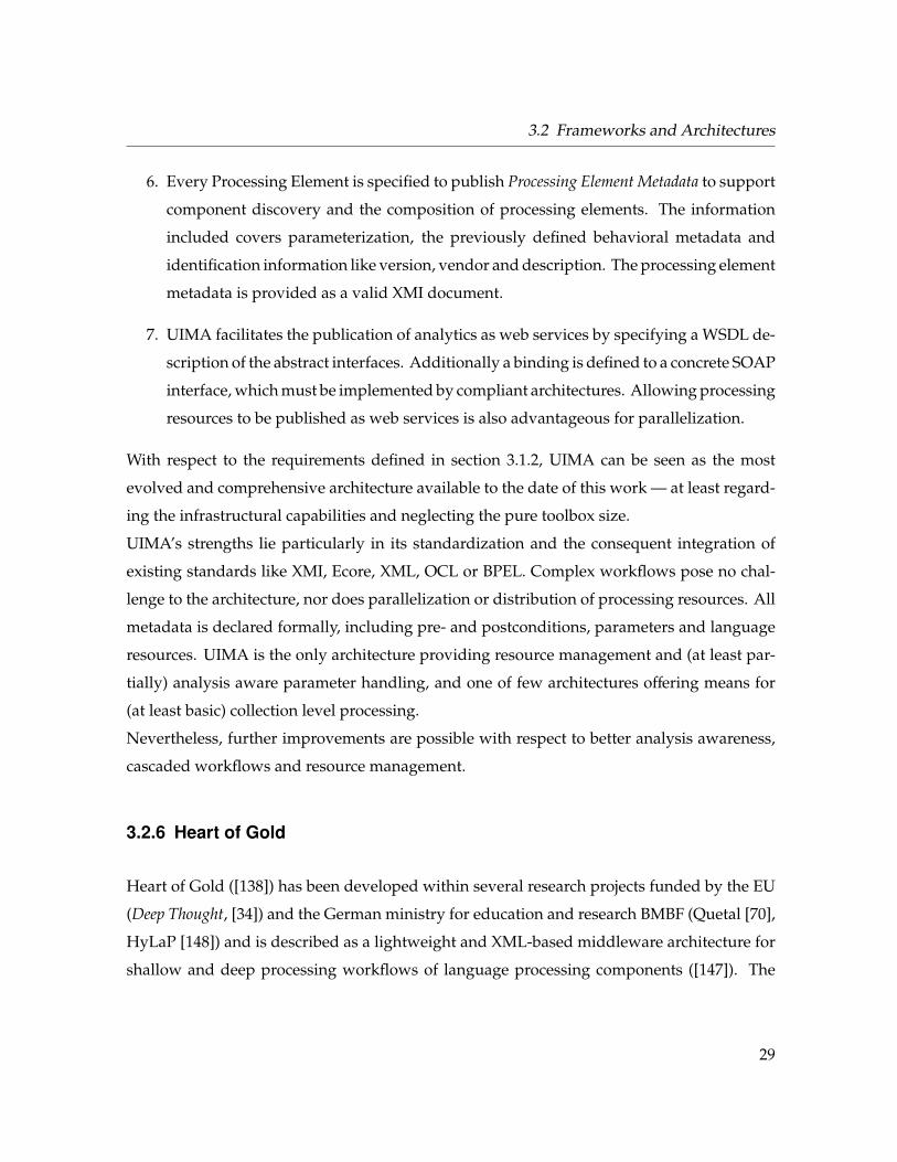
1. The Common Analysis Structure (CAS) is the common data structure shared by all UIMA
processing resources to represent the artifact as well as the corresponding annotations
(or metadata in general). The artifact is encapsulated in one or even more Subjects of
Analysis (Sofas). Similar to the GATE document model the CAS can be considered the
common interface for sharing data between all analytics with all contained objects being
modelled using the UIMA Type System (see below). Annotations are allowed to refer-
ence other annotations or objects in general, thereby allowing hierarchical structures
such as parse trees. According to the specification annotations may be enriched with
metadata about themselves such as confidence or provenance values and it is possible
to create views on the sofas. Import and export of CAS objects is achieved by using the
XML Metadata Interchange specification (XMI4). XMI was chosen because of being a
widespread standard and being aligned with object-oriented programming and UML.
2. Every CAS must conform to a user-defined type system, which is described within the
Type System Model. The design goal of data modeling and interchange is achieved by
specifying the used object model by the type system language. It is important to mention
that the UIMA framework does not include a particular set of types that developers
must use. The standard however mentions the need for a common set of type systems
([103, page 12]) for different domains or industrial usecases. The modeling language
used to define the Type System Model is the Ecore standard of the Eclipse Modeling
Framework (EMF5).
4http://www.omg.org/spec/XMI/5http://www.eclipse.org/modeling/emf/
27
3 Language Engineering Architectures
3. Although UIMA does not define specific type systems for analytics, it does define a Base
Type System containing some commonly used and domain independent types, thereby
allowing a fundamental level of interoperability between different modules. The Base
Type System contains among others primitive types as defined by Ecore, views and
general source document information like an URI pointing to the source document.
4. Abstract Interfaces are provided to define the standard component types and operations.
The supertype of all components is the Processing Element (PE) which basically provides
operations dealing with the component’s metadata and configuration parameters. This
supertype is inherited by three subtypes: Analyzers, CAS Multiplier and Flow Controllers.
Analyzers process the CAS and update its content with new or modified annotations
(similar to processing resources in GATE), while CAS multipliers are able to map a set of
input CASes to a set of output CASes by creating new ones or merging existent ones. An
important feature is the possibility of an analyzer to process a batch of CASes, thereby
providing the capability to do collection level processing. Flow Controllers determine
the route CASes take through a workflow of multiple analytics. By describing the
desired flow in a flow language like BPEL6 this results in a powerful, flexible and
reusable workflow management.
5. Every analytic describes its processing characteristics using Behavioral Metadata. This
metadata declaratively describes in terms of type system definitions prerequisites to
the CAS, which elements in the CAS are analyzed and in which way the CAS contents
are altered or modified. Using this information UIMA can automatically discover
required analytics and their composition can be supported by an automated process.
Additionally the metadata helps in facilitating efficient sharing of CAS content among
processing elements working together. Behavioral Metadata specifies required inputs
and the types of objects which may be created, modified or deleted. Although the UIMA
specification allows implementations to use any expression language to represent these
conditions, the specification defines a mapping to the Object Constraint Language (OCL7)
6http://docs.oasis-open.org/wsbpel/2.0/wsbpel-v2.0.html7http://www.omg.org/spec/OCL/2.2/
28
3.2 Frameworks and Architectures
6. Every Processing Element is specified to publish Processing Element Metadata to support
component discovery and the composition of processing elements. The information
included covers parameterization, the previously defined behavioral metadata and
identification information like version, vendor and description. The processing element
metadata is provided as a valid XMI document.
7. UIMA facilitates the publication of analytics as web services by specifying a WSDL de-
scription of the abstract interfaces. Additionally a binding is defined to a concrete SOAP
interface, which must be implemented by compliant architectures. Allowing processing
resources to be published as web services is also advantageous for parallelization.
With respect to the requirements defined in section 3.1.2, UIMA can be seen as the most
evolved and comprehensive architecture available to the date of this work — at least regard-
ing the infrastructural capabilities and neglecting the pure toolbox size.
UIMA’s strengths lie particularly in its standardization and the consequent integration of
existing standards like XMI, Ecore, XML, OCL or BPEL. Complex workflows pose no chal-
lenge to the architecture, nor does parallelization or distribution of processing resources. All
metadata is declared formally, including pre- and postconditions, parameters and language
resources. UIMA is the only architecture providing resource management and (at least par-
tially) analysis aware parameter handling, and one of few architectures offering means for
(at least basic) collection level processing.
Nevertheless, further improvements are possible with respect to better analysis awareness,
cascaded workflows and resource management.
3.2.6 Heart of Gold
Heart of Gold ([138]) has been developed within several research projects funded by the EU
(Deep Thought, [34]) and the German ministry for education and research BMBF (Quetal [70],
HyLaP [148]) and is described as a lightweight and XML-based middleware architecture for
shallow and deep processing workflows of language processing components ([147]). The
29
3 Language Engineering Architectures
Collection Processing Engine
CAS ConsumerCAS ConsumerText,
Video,Audio
CollectionReader
Aggregate Analysis Engine
Analysis Engine
Analysis Engine
Analysis Engine
Ontologies
Indices
Databases
KnowledgeBases
CAS Consumer
CASCAS CAS
Figure 3.1: The Unstructured Information Management Architecture (cp. [10, chapter 2.5.2])
Java based open source software is also contained in the OpenNLP8 toolbox.
The main architectural design principle behind Heart of Gold is the use of open XML stand-off
markup to represent the input and output of all components as it is easily exchangeable and
transformable using for example XSLT9. Furthermore unicode handling is directly provided
by the XML standard.
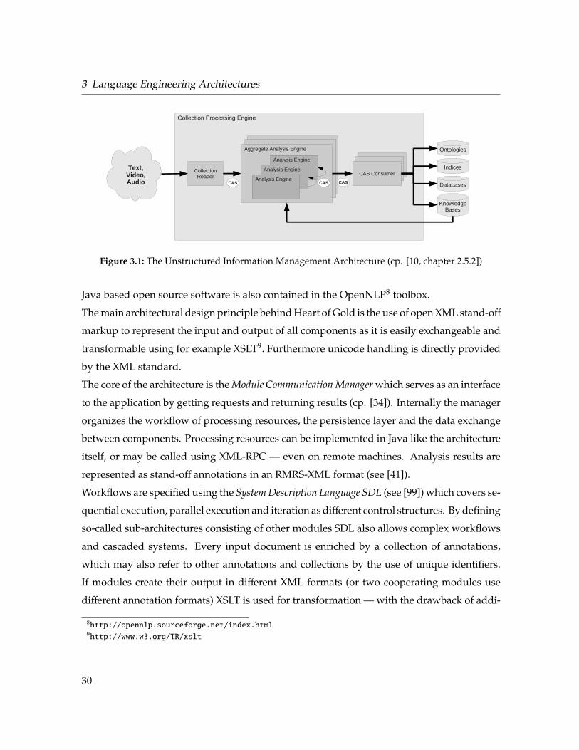
The core of the architecture is the Module Communication Manager which serves as an interface
to the application by getting requests and returning results (cp. [34]). Internally the manager
organizes the workflow of processing resources, the persistence layer and the data exchange
between components. Processing resources can be implemented in Java like the architecture
itself, or may be called using XML-RPC — even on remote machines. Analysis results are
represented as stand-off annotations in an RMRS-XML format (see [41]).
Workflows are specified using the System Description Language SDL (see [99]) which covers se-
quential execution, parallel execution and iteration as different control structures. By defining
so-called sub-architectures consisting of other modules SDL also allows complex workflows
and cascaded systems. Every input document is enriched by a collection of annotations,
which may also refer to other annotations and collections by the use of unique identifiers.
If modules create their output in different XML formats (or two cooperating modules use
different annotation formats) XSLT is used for transformation — with the drawback of addi-
8http://opennlp.sourceforge.net/index.html9http://www.w3.org/TR/xslt
30
3.2 Frameworks and Architectures
tional runtime. XSLT can also be utilized to combine and query annotations. The architecture
in general is depicted in figure 3.2.
Unfortunately Heart of Gold offers no capabilities for the definition of pre- and postconditions
and there is no parameter or resource management. Furthermore conditional workflows are
not supported by the architecture.
Application
XMLPersistenceFiles,
Database
ExternalProcessing Resources
ResultsQueries
SDL Workflow
InternalProcessing Resources
Module Communication Manager
AnnotationsXML, RMRS
XSLT
Figure 3.2: The Heart of Gold Middleware (cp. [147])
3.2.7 Other Architectures
A widespread and common toolbox is OpenNLP10, which considers itself to be "an umbrella
for various open source NLP projects to work with greater awareness and (potentially) greater
interoperability" (see [4]). With respect to this work OpenNLP is of minor importance, as it
does not define any infrastructural base, but is just a collection of perhaps even completely
different language processing tools.
10http://opennlp.sourceforge.net/index.html
31
3 Language Engineering Architectures
Another toolbox widely used is LingPipe, which sees itself as a "suite of Java libraries for
the linguistic analysis of human language" (see [8]. The Java based software includes a wide
range of machine learning algorithms for classification and clustering like k-means, SVM or
naive Bayes, but unfortunately does not provide an infrastructural architecture.
Other toolboxes and libraries which are freely available for research purposes but do not
provide sophisticated infrastructure capabilities beyond simple pipelines are FreeLing ([14]),
the UCLA NLP toolkit11, MontyLingua ([105]) and NLTK ([107]). Another toolkit which
provides more complex workflows and stand-off annotations is LinguaStream ([21]). A nice
set of information retrieval algorithms and tools can also be found in the Apache Lucene
project12.
3.2.8 Overview
An overview over a set of features selected with respect to application development is
presented in table 3.1.
3.2.9 Impact on Language Engineering
This chapter presented requirements for language engineering architectures and some of the
best known and wide-spread frameworks. The most promising infrastructures are based
on the TIPSTER document model, which allows flexible and structured enrichment of doc-
uments using typed stand-off annotations. Differences are especially given by the formal
declaration of resources. Definition of analysis aware conditions, parameters and resources
allow complex workflows, formal verifications and support to the user. Distributed and
parallel processing facilitates efficient applications, while the usage of standards enhances
the acceptance of the infrastructure itself.
While GATE is especially suitable for end-users because of the comprehensive toolbox and
11http://www.mii.ucla.edu/nlp/12http://lucene.apache.org/java/docs/index.html
32
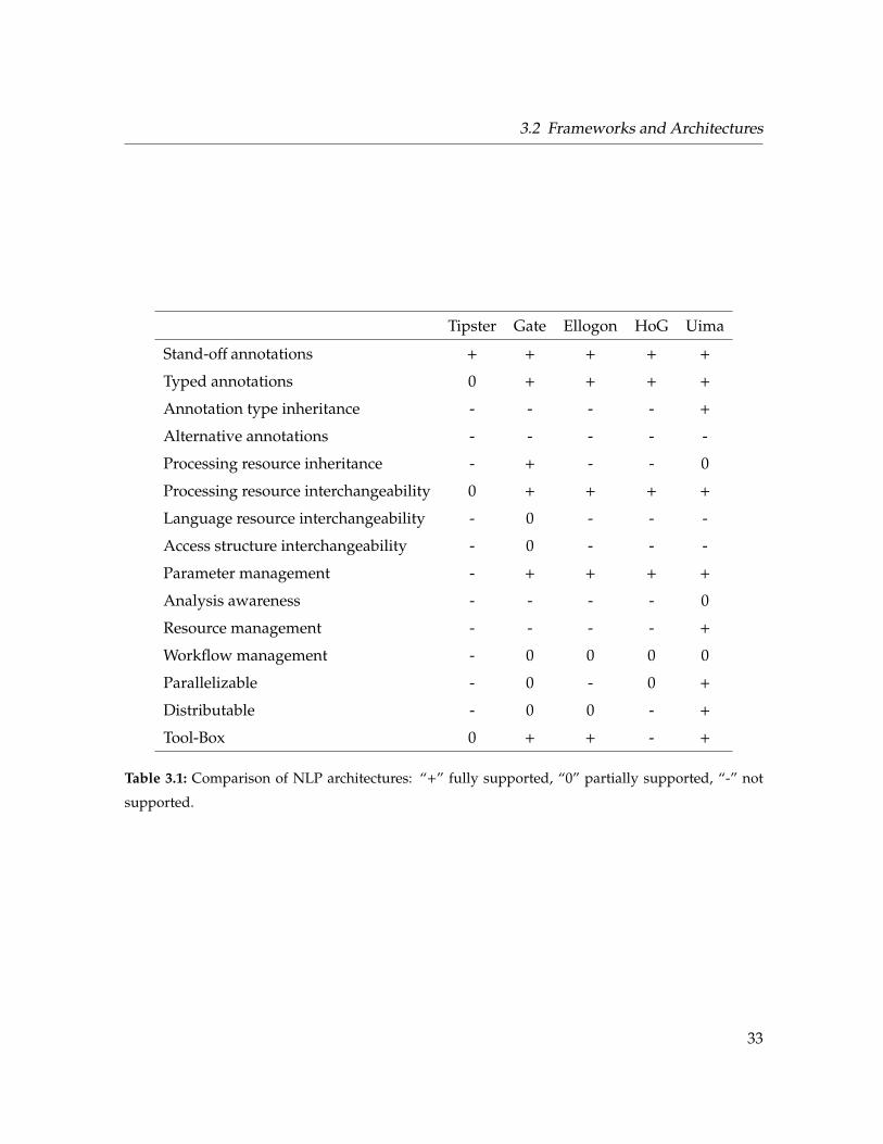
3.2 Frameworks and Architectures
Tipster Gate Ellogon HoG Uima
Stand-off annotations + + + + +
Typed annotations 0 + + + +
Annotation type inheritance - - - - +
Alternative annotations - - - - -
Processing resource inheritance - + - - 0
Processing resource interchangeability 0 + + + +
Language resource interchangeability - 0 - - -
Access structure interchangeability - 0 - - -
Parameter management - + + + +
Analysis awareness - - - - 0
Resource management - - - - +
Workflow management - 0 0 0 0
Parallelizable - 0 - 0 +
Distributable - 0 0 - +
Tool-Box 0 + + - +
Table 3.1: Comparison of NLP architectures: “+” fully supported, “0” partially supported, “-” not
supported.
33
3 Language Engineering Architectures
GUI tools, UIMA is the most promising architecture with respect to infrastructural capa-
bilities and performance concerns. This is due to the sophisticated workflow manage-
ment, resource distribution, resource parallelization and analysis aware metadata hand-
ling.
34
4 Language Characteristics
This chapter tries to define which language characteristics are of importance for the construc-
tion of information extraction systems and how they can be obtained and utilized. A text
understanding step should be performed as a first step of building such a system, and should
therefore be accomplished without the help of untrained language processing technologies.
The focus of this part is on simple measurements which can be calculated automatically or
with reasonable human effort, yet characterizing the domain language to an extend sufficient
for building an adequate information extraction system.
Language Statistics are used to measure and quantify certain characteristics of natural lan-
guage with statistical methods. This is in general useful to understand texts, corpora or
languages, but can also be interesting with respect to certain applications. Statistical data
regarding letter, word or syllable frequencies can be used to identify a particular author’s
style (e.g. [76]) or to measure the readability of text (using e.g. the Gunning fox index [69]).
In this chapter some general language statistics and laws obtained by quantitative lin-
guistics will be presented and considered with respect to domain language. Furthermore
some additional measurements will be introduced, which are of special interest regard-
ing information extraction and domain language. In contrast to other works dealing with
language statistics, this chapter will focus on simple measurements describing the char-
acteristics of a corpus, instead of analyzing specific terms, or comparing different cor-
pora.
35
4 Language Characteristics
4.1 Lexical Statistics
Lexical statistics belong to the most basic areas of language statistics, dealing with frequency
and distribution of words or collocations, their usage in text and language, and the regularities
of their occurrences (see [156, chapter 1.1]).
A large extend of works in lexical statistics are based on frequency lists, which are a very
simple, yet effective and useful language statistic. All distinct tokens ti of the corpus (or
just the tokens contained in a suitable dictionary) are listed with their according occurrence
frequency f (ti). By ordering the tokens with regards to decreasing f (ti), the rank r(ti) of a
token in the frequency list can be obtained. Besides frequency lists for the actual tokens
one can also create frequency lists for their stemmed form or their roots. The corpus size is
denoted with N and the vocabulary of the corpus with V.
Frequency lists are considered useful for different tasks like spelling correction (e.g. [140]),
calculation of co-occurrence significances (see [32]) or even stopword identification. Due to
the open character of a language L, a complete vocabulary listing is impossible to create.
By splitting a frequency list in ranges of high, medium and low frequency tokens, it uncovers
a more detailed view on the language and its syntax. Especially the area of very frequent
words (normally the ten most frequent words), consists mainly of so called function words
like prepositions, pronouns, auxiliary verbs, conjunctions, grammatical articles or particles.
Those words have no or little lexical meaning, and serve mainly for the syntax of the sentence
by expressing grammatical relationships (see [156, chapter 1.2.2.1]). Therefore their fraction
of the total amount of words contained in the corpus is of special interest, stating how much
effort the speaker or writer made to express grammar and syntax.
The zone of words with medium frequency are defined as words with r(ti) > 10 and f (ti) > 10,
and contains less frequent grammatical words like conjunctions or prepositions, frequent
verbs as well as adjectives and nouns. The zone of words with lower and lowest frequency
( f (ti) < 10) is mostly made up of adjectives, verbs, nouns and adverbs (see [156, chapter
1.2.2.3]).
According to [176] the product of the rank of a token and its frequency is approximately
36
4.1 Lexical Statistics
constant, and given by
r(ti) f (ti) ≈ k (4.1)
This is called the First Zipf Law. Although there are two more laws of Zipf, they will be
discarded here, as they are without impact on the following work.
The entropy as defined by Shannon (cp. [112, chapter 2.2.1]) measures the average amount of
information as given by the result of a random experiment. Applied to language statistics it
gives the mean amount of information of a token in the corpus. The formula given here is
normalized to the vocabulary size |V|:
H = −∑ti ∈ V
p(ti) log|V| p(ti) (4.2)
One measure which is of special interest with regard to methods based on word n-grams
is the Richness of vocabulary, which influences the size of language models (see section 7.2).
According to [156, chapter 1.2.3.3] this measure should be evaluated based on three distinct
corpus properties. These are partly based on meaningful words, which specifies the tokens
expressing meaning (nouns, adjectives, pronouns, verbs etc.) in contrast to function words
(conjunctions, prepositions etc.). The first measure is the size of vocabulary RVoc, which is given
by normalizing the vocabulary size |V| by the total text length Nm with respect to meaningful
words:
RVoc =|V|Nm
(4.3)
The second measure is the dispersion of vocabulary, which expresses the relative
amount of low frequency tokens (Vlow = {t|t ∈ V ∧ f (t) < 10}) in the vocabulary
V:
DVoc =|Vlow|
|V|(4.4)
The last measure which is part of the richness of vocabulary is the concentration of vocabulary
(see [156, chapter 1.2.3.3]), which is defined by the ratio between the length of the text Ntop
with respect to the most frequent tokens (Vtop = {t|t ∈ V ∧ r(t) < 10}) and the total length of
the corpus N:
CVoc =Ntop
N(4.5)
37
4 Language Characteristics
A last lexical statistic needs to be mentioned, which is of special interest with regard to
domain specific corpora like internet texts. This measure is the spelling accuracy SAVoc and
is defined by the amount of correctly spelled words NCor with respect to the corpus length
N:
SAVoc =NCor
N(4.6)
This measure can furthermore be divided with respect to realword errors and nonword
errors (see section 6.3) and influences crucially which kind of spellchecking method needs to
be employed.
4.2 Grammatical Statistics
Lexical statistics are focused on information about token frequencies or ratios with respect to
vocabulary or text length, thereby ignoring the syntax of words completely. To cover the
structure (resp. syntax) of a corpus, several measures dealing with part of speech tags, word
order and sentence length are now introduced.
Morphological statistics are interested in the frequency, distribution and relations of word forms
through their morphological categories (see [156, chapter 2.3.1]). For the sake of simplicity
this work will only consider a very basic and related statistic: Calculating the frequencies
fpos of the different parts of speech. As the text understanding step should be performed
initially on a new corpus, there will often be no reliable part of speech tagger available for an
automatic analysis. According to [156, chapter 2.3.1.2.2] it is however possible to create this
statistic on a sample of 500 to 1.500 words.
A second grammatical statistic is the corpus predictability, for which the entropy of a first order
Markov source is needed:
H(S) = −∑
i
pi
∑j
pi( j) log pi( j) (4.7)
38
4.2 Grammatical Statistics
The corpus predictability CP is calculated by normalizing the first order entropy with the
maximum possible entropy, and subtracting the result from 1:
CP = 1 −H(S)
Hmax(S)(4.8)
A high value of CP indicates a very straight-forward writing style with words often followed
by the same successors. This is an advantageous behavior for Hidden Markow Models, the
calculation of neighborhood co-occurrences and further language processing approaches.
A measure which is concerned with stating a (admittedly rudimentary) gram-
matical complexity GC is the ratio of function words N f to meaningful words
Nm:
GC =N f
Nm(4.9)
Although this rather basic approach cannot state a real level of grammatical structure of the
corpus, it still provides a good evidence for the amount of effort put into expressing syntax.
Together with the average length of sentences this measure may influence in which manner
(e.g. deep or shallow) the text needs to be processed.
Especially in very restricted domain languages words tend to be syntactically less ambiguous
than in more general languages, making it therefore easier to assign part of speech tags to
them. This is represented by calculating the syntactic ambiguity SA of a corpus by calculating
the average entropy of a token’s part of speech tags POS. A token ti occurring with only
one tag s j has an entropy (and therefore ambiguity) of zero, and gets higher values for more
syntactic classes being assigned to it with lesser probabilities:
SA = −1|V|
∑ti∈V
∑s j∈POS
p(s j|ti) log p(s j|ti) (4.10)
A high value of SA indicates possible problems for part of speech tagging, while low values
stand for easy (or even trivial) part of speech tagging.
The last grammatical statistic is concerned with sentence lengths, which influences parsing
as well as deep methods. The length |Si| of a sentence Si is defined by the amount of
contained tokens, and the average sentence length over all sentences S is used as an indica-
39
4 Language Characteristics
tor:
L(Si) =1|S|
∑Si∈S
|Si| (4.11)
4.3 Semantic Statistics
Semantic statistics as for example introduced in [156, chapter 3.1] study the frequencies and
distributions of meanings of units at different language levels, e.g. the lexical meanings and
the grammatical semantics. In contrast to this work the following measures are defined with
special respect to the task of information extraction. One drawback of these measures is that
there is up to now no reliable method available for automatic calculation.
The first measure to mention is the lexical ambiguity LA. It is defined correspondingly
to the syntactic ambiguity above by calculating the entropy of a token’s meanings M.
The lexical ambiguity LA of a corpus is defined as the average lexical ambiguity per to-
ken:
LA = −1|V|
∑ti∈V
∑m j∈M
p(m j|ti) log p(m j|ti) (4.12)
Intuitively it is clear that a high ratio of highly ambiguous tokens in the text complicates
the extraction of information out of the text massively. Corpora with only a few ambiguous
words having few meanings are much easier to process and handle. Unfortunately there
is no way to calculate this measure automatically, but even a rough manual estimate of the
value can be considered useful.
Entities, which needs to be extracted from text might occur redundantly. A high information
redundancy is advantageous by making it possible to use high precision algorithms with low
recall. The information redundancy is calculated as the average count of appearances f (in) of
every information fact in. What kind of information is relevant for this measure depends
on the application and may be Named Entities as well as relational tuples such as <Person,
Organization>.
Whenever one is concerned with developing a system for information extraction, one of the
first steps should be the research of how dense the information to be extracted is contained in
40
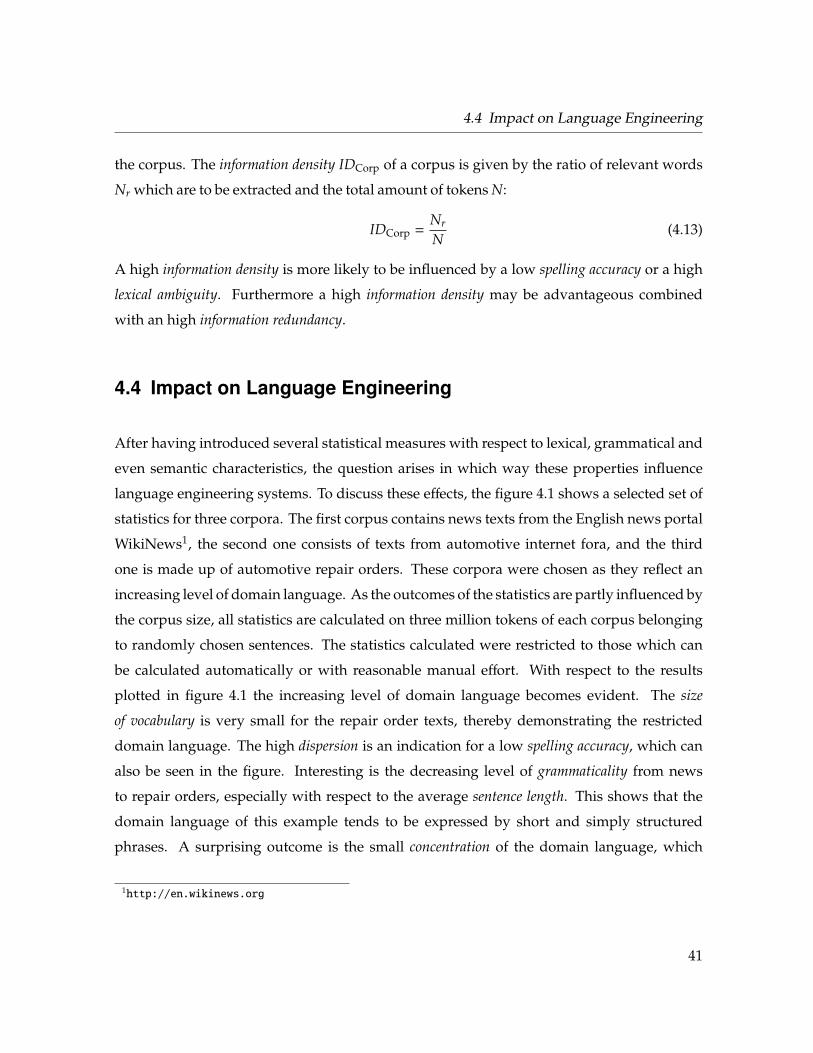
4.4 Impact on Language Engineering
the corpus. The information density IDCorp of a corpus is given by the ratio of relevant words
Nr which are to be extracted and the total amount of tokens N:
IDCorp =Nr
N(4.13)
A high information density is more likely to be influenced by a low spelling accuracy or a high
lexical ambiguity. Furthermore a high information density may be advantageous combined
with an high information redundancy.
4.4 Impact on Language Engineering
After having introduced several statistical measures with respect to lexical, grammatical and
even semantic characteristics, the question arises in which way these properties influence
language engineering systems. To discuss these effects, the figure 4.1 shows a selected set of
statistics for three corpora. The first corpus contains news texts from the English news portal
WikiNews1, the second one consists of texts from automotive internet fora, and the third
one is made up of automotive repair orders. These corpora were chosen as they reflect an
increasing level of domain language. As the outcomes of the statistics are partly influenced by
the corpus size, all statistics are calculated on three million tokens of each corpus belonging
to randomly chosen sentences. The statistics calculated were restricted to those which can
be calculated automatically or with reasonable manual effort. With respect to the results
plotted in figure 4.1 the increasing level of domain language becomes evident. The size
of vocabulary is very small for the repair order texts, thereby demonstrating the restricted
domain language. The high dispersion is an indication for a low spelling accuracy, which can
also be seen in the figure. Interesting is the decreasing level of grammaticality from news
to repair orders, especially with respect to the average sentence length. This shows that the
domain language of this example tends to be expressed by short and simply structured
phrases. A surprising outcome is the small concentration of the domain language, which
1http://en.wikinews.org
41
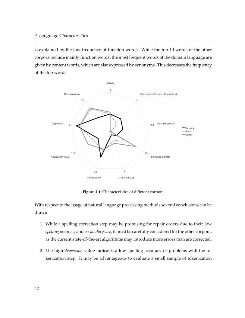
4 Language Characteristics
is explained by the low frequency of function words. While the top-10 words of the other
corpora include mainly function words, the most frequent words of the domain language are
given by content words, which are also expressed by synonyms. This decreases the frequency
of the top words.
Entropy
Concentration
Dispersion
Vocabulary Size
Predictability Grammaticality
Sentence Length
Misspelling Ratio
Information Density (Automotive)
RepairsForaNews
1
1
1
0.3
25
1
0.3
0.05
0.5
Figure 4.1: Characteristics of different corpora
With respect to the usage of natural language processing methods several conclusions can be
drawn:
1. While a spelling correction step may be promising for repair orders due to their low
spelling accuracy and vocabulary size, it must be carefully considered for the other corpora,
as the current state-of-the-art algorithms may introduce more errors than are corrected.
2. The high dispersion value indicates a low spelling accuracy or problems with the to-
kenization step. It may be advantageous to evaluate a small sample of tokenization
42
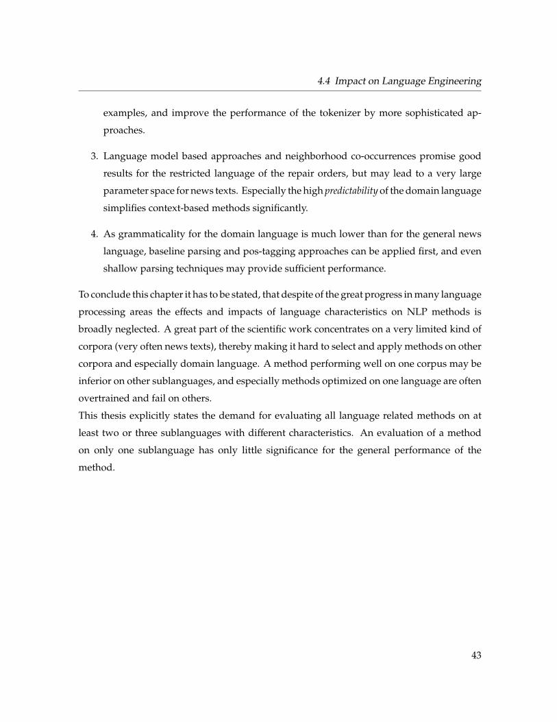
4.4 Impact on Language Engineering
examples, and improve the performance of the tokenizer by more sophisticated ap-
proaches.
3. Language model based approaches and neighborhood co-occurrences promise good
results for the restricted language of the repair orders, but may lead to a very large
parameter space for news texts. Especially the high predictability of the domain language
simplifies context-based methods significantly.
4. As grammaticality for the domain language is much lower than for the general news
language, baseline parsing and pos-tagging approaches can be applied first, and even
shallow parsing techniques may provide sufficient performance.
To conclude this chapter it has to be stated, that despite of the great progress in many language
processing areas the effects and impacts of language characteristics on NLP methods is
broadly neglected. A great part of the scientific work concentrates on a very limited kind of
corpora (very often news texts), thereby making it hard to select and apply methods on other
corpora and especially domain language. A method performing well on one corpus may be
inferior on other sublanguages, and especially methods optimized on one language are often
overtrained and fail on others.
This thesis explicitly states the demand for evaluating all language related methods on at
least two or three sublanguages with different characteristics. An evaluation of a method
on only one sublanguage has only little significance for the general performance of the
method.
43

44
5 Machine Learning for Language
Engineering
This chapter will present and outline some of the machine learning algorithms, which are
used widely for language engineering. As the same algorithm may be used for different
processing resources like sentence boundary detectors or named entity extractors, the baseline
algorithms with their advantages and shortcomings with respect to language engineering
will be discussed on their own. Chapter 6 about processing resources will refer to this
chapter.
5.1 Naive Bayes Classifier
The Naive Bayes Classifier is a Bayesian learning method which can be used to learn a target
function f (x) for a given instance x defined by a tuple of attribute values < a1, a2 . . . an > (cp.
[121, chapter 6.9]). After training the classifier on given training data it will be able to predict
the most probable target value VMAP (MAP stands for maximum a posteriori) of a finite set V
for a newly given instance xi:
VMAP = argmaxv j∈V
P(v j| a1, a2 . . . an) (5.1)
This equation can be transformed using Bayes’ Theorem, which provides means to calculate
a posterior probability P(h|D) of an hypothesis h and data D from a prior probability P(h) and
45
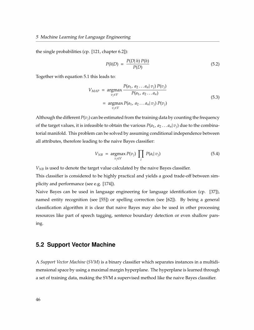
5 Machine Learning for Language Engineering
the single probabilities (cp. [121, chapter 6.2]):
P(h|D) =P(D| h) P(h)
P(D)(5.2)
Together with equation 5.1 this leads to:
VMAP = argmaxv j∈V
P(a1, a2 . . . an| v j) P(v j)P(a1, a2 . . . an)
= argmaxv j∈V
P(a1, a2 . . . an| v j) P(v j)(5.3)
Although the different P(v j) can be estimated from the training data by counting the frequency
of the target values, it is infeasible to obtain the various P(a1, a2 . . . an| v j) due to the combina-
torial manifold. This problem can be solved by assuming conditional independence between
all attributes, therefore leading to the naive Bayes classifier:
VNB = argmaxv j∈V
P(v j)∏
i
P(ai| v j) (5.4)
VNB is used to denote the target value calculated by the naive Bayes classifier.
This classifier is considered to be highly practical and yields a good trade-off between sim-
plicity and performance (see e.g. [174]).
Naive Bayes can be used in language engineering for language identification (cp. [37]),
named entity recognition (see [55]) or spelling correction (see [62]). By being a general
classification algorithm it is clear that naive Bayes may also be used in other processing
resources like part of speech tagging, sentence boundary detection or even shallow pars-
ing.
5.2 Support Vector Machine
A Support Vector Machine (SVM) is a binary classifier which separates instances in a multidi-
mensional space by using a maximal margin hyperplane. The hyperplane is learned through
a set of training data, making the SVM a supervised method like the naive Bayes classifier.
46
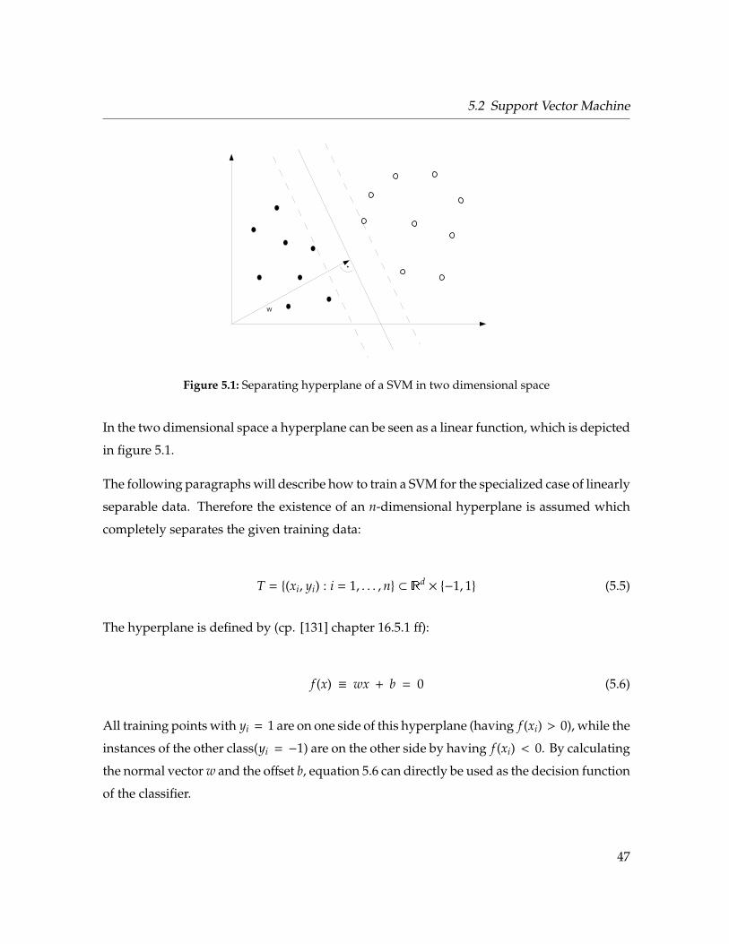
5.2 Support Vector Machine
w
Figure 5.1: Separating hyperplane of a SVM in two dimensional space
In the two dimensional space a hyperplane can be seen as a linear function, which is depicted
in figure 5.1.
The following paragraphs will describe how to train a SVM for the specialized case of linearly
separable data. Therefore the existence of an n-dimensional hyperplane is assumed which
completely separates the given training data:
T = {(xi, yi) : i = 1, . . . ,n} ⊂ Rd× {−1, 1} (5.5)
The hyperplane is defined by (cp. [131] chapter 16.5.1 ff):
f (x) ≡ wx + b = 0 (5.6)
All training points with yi = 1 are on one side of this hyperplane (having f (xi) > 0), while the
instances of the other class(yi = −1) are on the other side by having f (xi) < 0. By calculating
the normal vector w and the offset b, equation 5.6 can directly be used as the decision function
of the classifier.
47
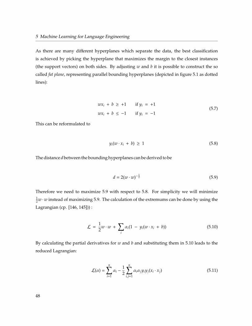
5 Machine Learning for Language Engineering
As there are many different hyperplanes which separate the data, the best classification
is achieved by picking the hyperplane that maximizes the margin to the closest instances
(the support vectors) on both sides. By adjusting w and b it is possible to construct the so
called fat plane, representing parallel bounding hyperplanes (depicted in figure 5.1 as dotted
lines):
wxi + b ≥ +1 if yi = +1
wxi + b ≤ −1 if yi = −1(5.7)
This can be reformulated to
yi(w · xi + b) ≥ 1 (5.8)
The distance d between the bounding hyperplanes can be derived to be
d = 2(w · w)−12 (5.9)
Therefore we need to maximize 5.9 with respect to 5.8. For simplicity we will minimize12 w ·w instead of maximizing 5.9. The calculation of the extremums can be done by using the
Lagrangian (cp. [146, 145])) :
L =12
w · w +∑
i
αi(1 − yi(w · xi + b)) (5.10)
By calculating the partial derivatives for w and b and substituting them in 5.10 leads to the
reduced Lagrangian:
L(α) =
n∑i=1
αi −12
n∑i, j=1
αiα jyiy j(xi · x j) (5.11)
48
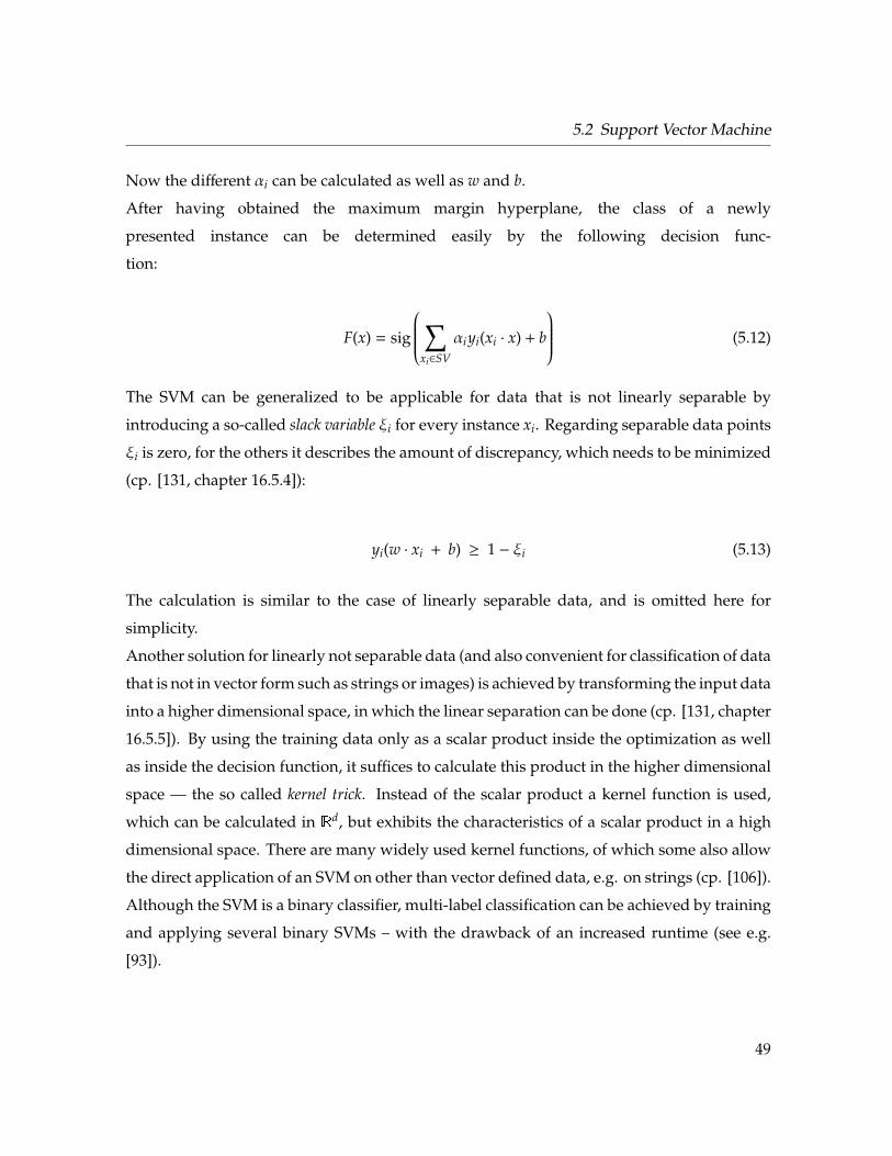
5.2 Support Vector Machine
Now the different αi can be calculated as well as w and b.
After having obtained the maximum margin hyperplane, the class of a newly
presented instance can be determined easily by the following decision func-
tion:
F(x) = sig
∑xi∈SV
αiyi(xi · x) + b
(5.12)
The SVM can be generalized to be applicable for data that is not linearly separable by
introducing a so-called slack variable ξi for every instance xi. Regarding separable data points
ξi is zero, for the others it describes the amount of discrepancy, which needs to be minimized
(cp. [131, chapter 16.5.4]):
yi(w · xi + b) ≥ 1 − ξi (5.13)
The calculation is similar to the case of linearly separable data, and is omitted here for
simplicity.
Another solution for linearly not separable data (and also convenient for classification of data
that is not in vector form such as strings or images) is achieved by transforming the input data
into a higher dimensional space, in which the linear separation can be done (cp. [131, chapter
16.5.5]). By using the training data only as a scalar product inside the optimization as well
as inside the decision function, it suffices to calculate this product in the higher dimensional
space — the so called kernel trick. Instead of the scalar product a kernel function is used,
which can be calculated in Rd, but exhibits the characteristics of a scalar product in a high
dimensional space. There are many widely used kernel functions, of which some also allow
the direct application of an SVM on other than vector defined data, e.g. on strings (cp. [106]).
Although the SVM is a binary classifier, multi-label classification can be achieved by training
and applying several binary SVMs – with the drawback of an increased runtime (see e.g.
[93]).
49
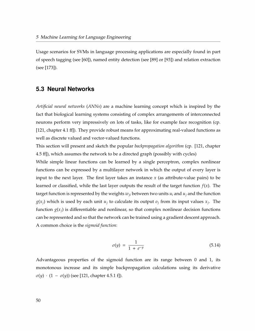
5 Machine Learning for Language Engineering
Usage scenarios for SVMs in language processing applications are especially found in part
of speech tagging (see [60]), named entity detection (see [89] or [93]) and relation extraction
(see [173]).
5.3 Neural Networks
Artificial neural networks (ANNs) are a machine learning concept which is inspired by the
fact that biological learning systems consisting of complex arrangements of interconnected
neurons perform very impressively on lots of tasks, like for example face recognition (cp.
[121, chapter 4.1 ff]). They provide robust means for approximating real-valued functions as
well as discrete valued and vector-valued functions.
This section will present and sketch the popular backpropagation algorithm (cp. [121, chapter
4.5 ff]), which assumes the network to be a directed graph (possibly with cycles)
While simple linear functions can be learned by a single perceptron, complex nonlinear
functions can be expressed by a multilayer network in which the output of every layer is
input to the next layer. The first layer takes an instance x (as attribute-value pairs) to be
learned or classified, while the last layer outputs the result of the target function f (x). The
target function is represented by the weights w ji between two units ui and u j and the function
g(x j) which is used by each unit u j to calculate its output o j from its input values x j. The
function g(x j) is differentiable and nonlinear, so that complex nonlinear decision functions
can be represented and so that the network can be trained using a gradient descent approach.
A common choice is the sigmoid function:
σ(y) =1
1 + e−y (5.14)
Advantageous properties of the sigmoid function are its range between 0 and 1, its
monotonous increase and its simple backpropagation calculations using its derivative
σ(y) · (1 − σ(y)) (see [121, chapter 4.5.1 f]).
50
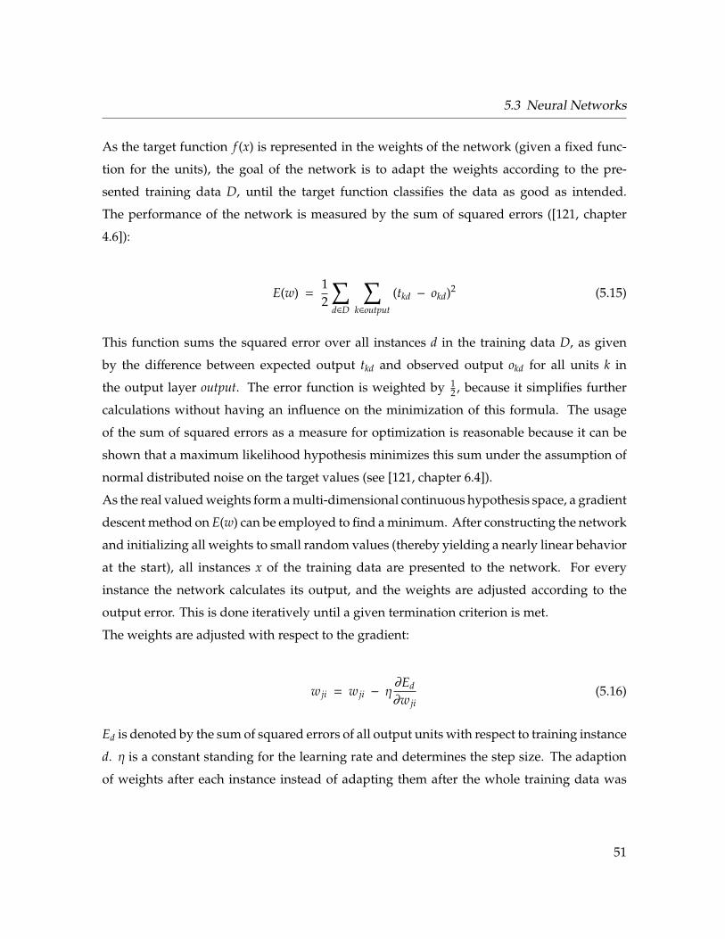
5.3 Neural Networks
As the target function f (x) is represented in the weights of the network (given a fixed func-
tion for the units), the goal of the network is to adapt the weights according to the pre-
sented training data D, until the target function classifies the data as good as intended.
The performance of the network is measured by the sum of squared errors ([121, chapter
4.6]):
E(w) =12
∑d∈D
∑k∈output
(tkd − okd)2 (5.15)
This function sums the squared error over all instances d in the training data D, as given
by the difference between expected output tkd and observed output okd for all units k in
the output layer output. The error function is weighted by 12 , because it simplifies further
calculations without having an influence on the minimization of this formula. The usage
of the sum of squared errors as a measure for optimization is reasonable because it can be
shown that a maximum likelihood hypothesis minimizes this sum under the assumption of
normal distributed noise on the target values (see [121, chapter 6.4]).
As the real valued weights form a multi-dimensional continuous hypothesis space, a gradient
descent method on E(w) can be employed to find a minimum. After constructing the network
and initializing all weights to small random values (thereby yielding a nearly linear behavior
at the start), all instances x of the training data are presented to the network. For every
instance the network calculates its output, and the weights are adjusted according to the
output error. This is done iteratively until a given termination criterion is met.
The weights are adjusted with respect to the gradient:
w ji = w ji − η∂Ed
∂w ji(5.16)
Ed is denoted by the sum of squared errors of all output units with respect to training instance
d. η is a constant standing for the learning rate and determines the step size. The adaption
of weights after each instance instead of adapting them after the whole training data was
51
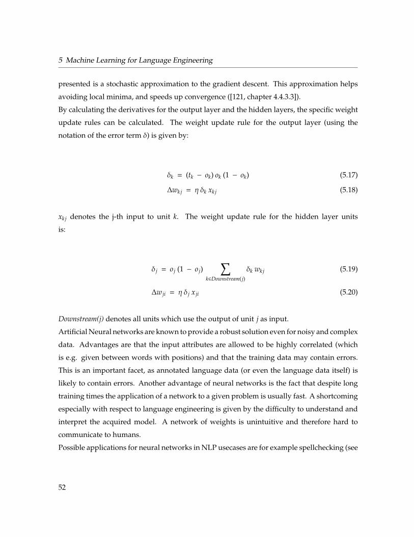
5 Machine Learning for Language Engineering
presented is a stochastic approximation to the gradient descent. This approximation helps
avoiding local minima, and speeds up convergence ([121, chapter 4.4.3.3]).
By calculating the derivatives for the output layer and the hidden layers, the specific weight
update rules can be calculated. The weight update rule for the output layer (using the
notation of the error term δ) is given by:
δk = (tk − ok) ok (1 − ok) (5.17)
∆wkj = η δk xkj (5.18)
xkj denotes the j-th input to unit k. The weight update rule for the hidden layer units
is:
δ j = o j (1 − o j)∑
k∈Downstream( j)
δk wkj (5.19)
∆w ji = η δ j x ji (5.20)
Downstream(j) denotes all units which use the output of unit j as input.
Artificial Neural networks are known to provide a robust solution even for noisy and complex
data. Advantages are that the input attributes are allowed to be highly correlated (which
is e.g. given between words with positions) and that the training data may contain errors.
This is an important facet, as annotated language data (or even the language data itself) is
likely to contain errors. Another advantage of neural networks is the fact that despite long
training times the application of a network to a given problem is usually fast. A shortcoming
especially with respect to language engineering is given by the difficulty to understand and
interpret the acquired model. A network of weights is unintuitive and therefore hard to
communicate to humans.
Possible applications for neural networks in NLP usecases are for example spellchecking (see
52
5.4 Decision Trees
[101, section 2.2.6]), part of speech tagging (see [143]) or Named Entity classification (cp. [55]).
However, other machine learning algorithms seem to be preferred by the NLP community
— perhaps due to the black-box nature of neural networks, which make it hard to manually
modify or adapt the acquired models. Another reason may be found in the high number
of features (dictionary size, tagset size, etc.) often found in language processing scenarios,
which leads to huge input or output layers.
5.4 Decision Trees
A commonly used and practical method for approximating discrete-valued target functions
is the creation of so-called decision trees ([121, chapter 3 ff]). A decision tree represents the
target function in form of a tree, in which every node tests one (or more) attributes of the input
instance. Each of the branches of such a node represents a different value of this attribute.
Classification of a new instance is achieved by testing its attributes downwards along the
tree, thereby reaching a leaf with the (hopefully) correct classification ([121, chapter 3.2 f]).
While each path from the root to a given leaf can be seen as a conjunction of attribute tests,
the tree as a whole expresses the disjunction of these conjunctions. Therefore decision trees
can also be formulated as sets of if-then rules, which is easy to understand, interpret and
apply for human users.
The construction of a decision tree will be explained using the rather basic ID3 algorithm
([133], [121, chapter 3.4]) to which several extensions and improvements exist and which
therefore forms the basis for many decision tree algorithms.
The ID3 algorithm can be seen as a top-down and greedy search through the hypothesis space
of possible decision trees ([121, chapter 3.4]), but without the use of backtracking. For every
node of the tree (down from the root) the remaining attributes are considered and evaluated
using a statistical measure, the information gain. In each step, the attribute providing the
highest information gain is chosen, and the tree is branched with respect to its values. The
measure of information gain is based on the entropy of a collection of training instances
53
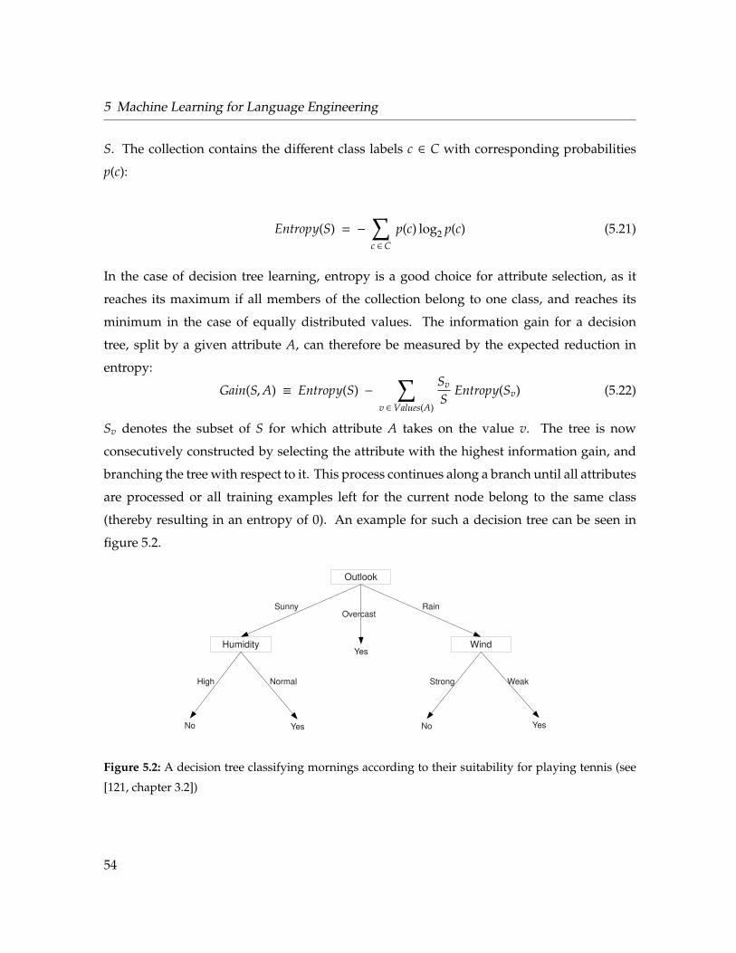
5 Machine Learning for Language Engineering
S. The collection contains the different class labels c ∈ C with corresponding probabilities
p(c):
Entropy(S) = −∑c ∈ C
p(c) log2 p(c) (5.21)
In the case of decision tree learning, entropy is a good choice for attribute selection, as it
reaches its maximum if all members of the collection belong to one class, and reaches its
minimum in the case of equally distributed values. The information gain for a decision
tree, split by a given attribute A, can therefore be measured by the expected reduction in
entropy:
Gain(S,A) ≡ Entropy(S) −∑
v ∈ Values(A)
Sv
SEntropy(Sv) (5.22)
Sv denotes the subset of S for which attribute A takes on the value v. The tree is now
consecutively constructed by selecting the attribute with the highest information gain, and
branching the tree with respect to it. This process continues along a branch until all attributes
are processed or all training examples left for the current node belong to the same class
(thereby resulting in an entropy of 0). An example for such a decision tree can be seen in
figure 5.2.
WindHumidity
Outlook
Sunny Rain
Yes
Overcast
Yes YesNoNo
High Normal Strong Weak
Figure 5.2: A decision tree classifying mornings according to their suitability for playing tennis (see
[121, chapter 3.2])
54
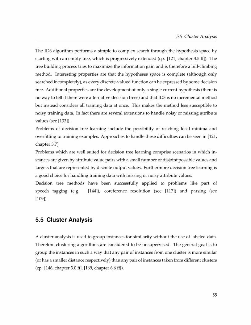
5.5 Cluster Analysis
The ID3 algorithm performs a simple-to-complex search through the hypothesis space by
starting with an empty tree, which is progressively extended (cp. [121, chapter 3.5 ff]). The
tree building process tries to maximize the information gain and is therefore a hill-climbing
method. Interesting properties are that the hypotheses space is complete (although only
searched incompletely), as every discrete-valued function can be expressed by some decision
tree. Additional properties are the development of only a single current hypothesis (there is
no way to tell if there were alternative decision trees) and that ID3 is no incremental method
but instead considers all training data at once. This makes the method less susceptible to
noisy training data. In fact there are several extensions to handle noisy or missing attribute
values (see [133]).
Problems of decision tree learning include the possibility of reaching local minima and
overfitting to training examples. Approaches to handle these difficulties can be seen in [121,
chapter 3.7].
Problems which are well suited for decision tree learning comprise scenarios in which in-
stances are given by attribute value pairs with a small number of disjoint possible values and
targets that are represented by discrete output values. Furthermore decision tree learning is
a good choice for handling training data with missing or noisy attribute values.
Decision tree methods have been successfully applied to problems like part of
speech tagging (e.g. [144]), coreference resolution (see [117]) and parsing (see
[109]).
5.5 Cluster Analysis
A cluster analysis is used to group instances for similarity without the use of labeled data.
Therefore clustering algorithms are considered to be unsupervised. The general goal is to
group the instances in such a way that any pair of instances from one cluster is more similar
(or has a smaller distance respectively) than any pair of instances taken from different clusters
(cp. [146, chapter 3.0 ff], [169, chapter 6.6 ff]).
55
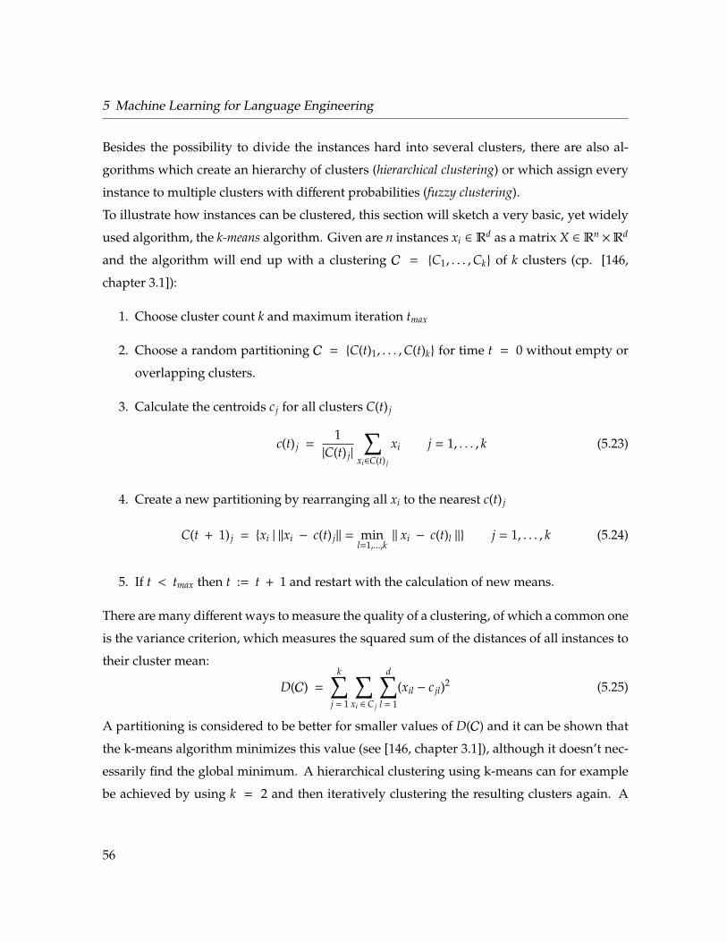
5 Machine Learning for Language Engineering
Besides the possibility to divide the instances hard into several clusters, there are also al-
gorithms which create an hierarchy of clusters (hierarchical clustering) or which assign every
instance to multiple clusters with different probabilities (fuzzy clustering).
To illustrate how instances can be clustered, this section will sketch a very basic, yet widely
used algorithm, the k-means algorithm. Given are n instances xi ∈ Rd as a matrix X ∈ Rn
×Rd
and the algorithm will end up with a clustering C = {C1, . . . ,Ck} of k clusters (cp. [146,
chapter 3.1]):
1. Choose cluster count k and maximum iteration tmax
2. Choose a random partitioning C = {C(t)1, . . . ,C(t)k} for time t = 0 without empty or
overlapping clusters.
3. Calculate the centroids c j for all clusters C(t) j
c(t) j =1|C(t) j|
∑xi∈C(t) j
xi j = 1, . . . , k (5.23)
4. Create a new partitioning by rearranging all xi to the nearest c(t) j
C(t + 1) j = {xi | ||xi − c(t) j|| = minl=1,...,k
|| xi − c(t)l ||} j = 1, . . . , k (5.24)
5. If t < tmax then t := t + 1 and restart with the calculation of new means.
There are many different ways to measure the quality of a clustering, of which a common one
is the variance criterion, which measures the squared sum of the distances of all instances to
their cluster mean:
D(C) =
k∑j = 1
∑xi ∈ C j
d∑l = 1
(xil − c jl)2 (5.25)
A partitioning is considered to be better for smaller values of D(C) and it can be shown that
the k-means algorithm minimizes this value (see [146, chapter 3.1]), although it doesn’t nec-
essarily find the global minimum. A hierarchical clustering using k-means can for example
be achieved by using k = 2 and then iteratively clustering the resulting clusters again. A
56
5.5 Cluster Analysis
fuzzy clustering is created by using the distinct distances to the different cluster means to
calculate the fuzzy membership to the corresponding cluster.
If there are no instances given but only a distance (or similarity) matrix, graph clustering
methods can be utilized which consider the similarity matrix as a graph, and cluster it by
using graph algorithms. Graph Clustering tries to break a given graph into meaningful sub-
graphs, normally in a way so that the vertices in the subgraphs are strongly connected to each
other, yet having only few edges to other subgraphs (or edges with high weights within the
subgraphs, and few edges with small weights to other subgraphs). Although some vector
cluster algorithms can be applied to graphs, there is also a set of so called graph clustering
algorithms, which use methods and ideas from graph theory, like the minimum cut or mini-
mal spanning trees, to find clusters in a graph.
A very fast graph cluster algorithm is the Chinese Whispers algorithm, which can be seen as
a special version of the MCL algorithm (see [161]), yet being more effective (O(|E|), which is
especially fine for sparse graphs) and parameter-free (see [18]).
After initially assigning each vertex in a graph a different class label, the algorithm will itera-
tively go through all vertices in a randomized order, and assign each vertex the predominant
class label in its neighborhood. The algorithm stops after a small amount of iterations, or if
convergence is reached. The drawback of this algorithm is its randomized and indetermin-
istic behavior.
Clustering methods are broadly used in language processing systems and provide means
for e.g. word sense discrimination (see [151]) or unsupervised part of speech tagging (see
[16]).
57

58
6 Processing Resources
There is a broad consensus in the scientific community that information extraction systems
consist of a workflow of different modules, normally sequentially arranged. This chapter
describes and analyzes common processing resources for the implementation of an infor-
mation extraction system and classifies them with respect to given criteria. Every module
will be analyzed with regard to a special set of characteristics, which are important in the
design phase of any information extraction process. These characteristics cover the require-
ments given to use this module, its dependencies to other modules and basic infrastructural
questions.
1. Basic necessity: One of the most important questions when choosing modules for
an information extraction system is the question which modules are necessary and
how much surplus value they generate in comparison to the price of their usage.
A language identification step for example may be worthless, if the ratio of foreign
language documents is smaller than the error rate of the language identification module.
2. Dependencies: The dependencies of a module are given by its input requirements to
fulfill its task. Most syntax parsers for example require part of speech tagged input,
while the part of speech tagger on the other hand relies on tokenized input itself.
Although dependencies are in fact related to the method instead of the module, this
issue will be treated on a module level for simplicity. Especially interesting with respect
to language engineering are mutual dependencies, which may be hard to resolve (see
section 8.2).
59
6 Processing Resources
3. Infrastructure: Infrastructural questions are related to the kind of annotations used,
distributed or parallel execution, workflow related questions and resource management
of this module.
While the module itself is merely interesting for architectural decisions, the method used in
the module is of high importance for the usage of the system as a whole. Characteristics of
a method include the initial effort to use this method, its runtime and the accuracy, which
can be achieved. But besides that, there are further characteristics, which are often neglected
in other scientific work, but have a strong impact on any real world application. These
include the robustness of the algorithm being confronted with erroneous or noisy input, or
the generality of the method.
1. Initial effort: The initial effort of a method describes the amount of time that is needed to
get the method going on one specific language. This involves the creation of resources,
the annotation of training data and the optimization of parameters. The initial effort
to create an information extraction system for a given sublanguage is the sum of the
initial efforts for all modules — or even less, if training data or language resources (e.g.
dictionaries) can be shared and reused.
2. Robustness: The robustness of a system is given by its ability to handle erroneous,
unexpected or noisy input. Methods with a lack of robustness may generate erroneous
output under these conditions, or may increase runtime significantly. Given a sequential
workflow of information extraction modules, the robustness of the system as a whole is
expected to be below the weakest component, due to cumulative effects. This problem
increases the earlier the weakest module is executed in the workflow.
3. Maintainability: The maintainability of a module is given by the possibilities it offers to
an information extraction engineer to adapt it to other sublanguages (see initial effort)
and to keep it up to date to changes in the input data, like new terms, changes in syntax
or changes in the module dependencies.
60
6.1 Language Identification
4. Generality: The generality of a module describes its ability to be trained on one sublan-
guage and applied to another. Although this might not seem to be sensible, it is a great
assistance to be able to use an existing method as-is on other kinds of data, without the
need of changes and retraining.
5. Performance: The performance of a specific method is given by the accuracy of its
output in comparison to the aspired targets. Performance is normally measured in
terms of accuracy, precision or recall, and is exhaustively covered in other scientific
work.
6. Runtime Complexity: The runtime complexity of a method describes the speed of the
applied method, and especially the growth of runtime related to the problem size (very
often the number of tokens etc.).
As it is obvious that it is infeasible to cover all these properties for all methods and modules
available (especially as most of them are impossible to prove in a formal way, and even
the empirical evaluation would be too time consuming), the following sections try to rely
on existing literature and experiments. Although this implies that not everything can be
answered, this overview will be as comprehensive as possible.
6.1 Language Identification
Language Identification (LI) denotes the task of assigning the proper language to a piece of
text of arbitrary size. As it is obviously no problem to compile suitable training data of text
labeled with the right language code, language identification can be seen as a good task for
supervised classification algorithms like the ones listed in chapter 5. And in fact there are
solutions using for example support vector machines (see [100]) or Bayesian models (see
[51]).
Much more interesting with respect to language identification is the question which features
should be used to accomplish this task. Although advanced features like part of speech tags
61
6 Processing Resources
or parse trees would be useful to detect the right language, it is evident that the calculation of
those features depends on the language of the text, and that they are therefore impossible to
use. In fact nearly all processing resources of a language processing system rely on language
information to load the right language resources and parameters, thereby leading to the
assumption that language identification needs to be accomplished as one of the first steps of
every workflow. Therefore only the most basic features can be used, involving characters,
words and their corresponding n-grams.
The usage of words (and word n-grams respectively) is exemplary shown in [20], but has
different shortcomings as discussed in [51] or [114]:
1. The usage of words as features implies the usage of a tokenizer (see section 6.2). This
leads to two problems. Firstly the tokenization itself may be complicated or error prone
(as in Chinese), secondly tokenization should be performed language aware itself to
handle special cases or Asian languages.
2. Especially brief texts or texts from a specialized domain may not even contain common
words from the language profiles. It is apparent that two English texts from different
domains share more character n-grams than words.
3. Word based approaches suffer from the influence of inflections and compounds and
are especially weak with regard to polysynthetic languages. Although this could be
solved by lexical or morphological analysis, this analysis would again need to know
the language — and introduces new error sources.
4. Language identification based on words is susceptible to spelling errors like for example
introduced by optical character recognition (OCR) methods. Although these could be
corrected using a spellchecker, the spelling correction itself would need to know the
language of the text.
5. Language identification using words mainly profits from frequent words, which are
normally functional words like determiners, prepositions or conjunctions. As those
62
6.1 Language Identification
words are normally short, they are also contained in character n-grams and are therefore
also incorporated in character n-gram solutions.
Although word-based methods are known to yield good performance (even the usage of the
most frequent words is often sufficient) they can be seen as less robust and general than char-
acter n-gram based methods. Furthermore they pose additional infrastructural problems by
introducing mutual dependencies to e.g. a tokenizer or a morphological analyzer. Therefore
newer approaches are consequently based on character n-grams (see [37], [100] or [153]). The
predominant approach is as follows:
1. Create a character n-gram profile Pl for every language l in the training data and fill it
with n-grams ni and their probabilities.
2. Create a corresponding profile Pt for every text t which has to be classified.
3. Compare the text profiles to the language profiles of the training data using a similarity
measure S. Probabilities calculated by smoothing techniques can be assigned to n-grams
missing in the training data (see [112, chapter 6.2.1 ff]).
4. Assign the language code to the text, which fits the profile best. If there are several
profiles with similar results, the language identifier can also output unknown or the
probability distribution for all language codes.
There are several similarity measures proposed for the comparison of n-gram profiles. [37]
defines a simple measure based on the sum of the rank differences of the n-grams in the two
profiles:
SRank(Pl,Pt) =∑
ni ∈ Pt
| RankPl(ni) − RankPt(ni) | (6.1)
Another measure based on entropy is used by [153] and outperforms the sim-
ple rank metric. In this approach the distance is calculated instead of a similar-
ity:
DEntropy(Pl,Pt) =∑
ni ∈ Pt
pt(ni) logpt(ni)pl(ni)
(6.2)
63
6 Processing Resources
pt(ni) denotes the probability of the n-gram ni in the profile for text t.
One shortcoming of these approaches is the omission of positions. An approach being more
sophisticated than those bag of n-gram models is the method proposed by [51]. String order is
preserved by using a Markov Model for every language in the training data, and calculating
the probabilities for a given text to be generated by those models. The probability for a text S
(having tokens si) to be created by a model A is calculated by:
p(S | A) = p(s1, . . . , sk | A)N∏
i = k + 1
p(si | si − k, . . . , si − 1 | A) (6.3)
With regard to the literature, it can be said that all these approaches perform very well. A
direct comparison is difficult as every research group uses text from different domains (web
pages, newsgroups) and different amounts of target languages to identify. However, the
literature agrees that the n-gram based approaches easily achieve classification accuracies
above 99% (see [153], [37] or [51]), if there is a reasonable amount of training data (e.g. >
5.000 characters) and the text is not too short (say several lines of text). Considering the fact
that it is easy to construct large training data and texts to classify are normally long, it is
understandable that language identification is often seen as a solved problem. But especially
with respect to brief texts and multilingual documents this is not the case. Short texts lead
to lower classification rates (e.g. 90.7% for one line of text and 2000 lines of training data
in [153]) and texts made up of samples of different languages may be classified completely
wrong (a nice example is given in [71]). Right now there are not many solutions given to
multilingual texts. An interesting approach suggested by [71] achieves 19.3% accuracy in an
(admittedly very complicated) setting of tuples containing four words in three languages.
With respect to language engineering one can state that n-gram based methods are preferable.
They combine robust and very efficient means to detect the language of a given text with a
good generalization behavior. The initial effort for the construction of training data is very
low as training data can be taken from other domains and several hundred lines of text are
sufficient. Furthermore there are unsupervised methods for the creation of training data
available as described in [20]. The suggested method is robust with respect to spelling errors
and morphology and the maintainability is good as the method is general enough to be nearly
64
6.2 Tokenization
maintenance free. If the texts are however short or multilingual, the performance needs to
be evaluated and methods might need to be switched — but up to now there is a lack of high
accuracy methods for these cases.
With respect to the language engineering architecture it has to be stated that a language
identification module makes sense if the amount of different languages in the analysis corpora
is higher than the error rate of the method used. Considering the current state of the art,
this means that a language identification step should be employed if at least several percent
of the corpus is written in different languages. Language identification has no considerable
input dependencies but serves as a basis for nearly every upcoming step. It has mutual
dependencies to the tokenizer (if the language identification method is word-based) and
sentence boundary detection (if language is annotated on a sentence level). If it is possible to
segment words and sentences of the languages found in the corpus with the same methods
and parameters, language identification can be performed after those modules. Weaker
mutual dependencies are found to Named Entity Recognition and Quote Recognition. Named
entities and quotes are often written in different languages and therefore influence language
identification performance. Quotes can be identified reliably, if language identification is
done on a sentence or paragraph level. Getting the language of named entities right is hard,
but might not be necessary given the application context, as long as the surrounding text is
identified correctly.
Regarding type systems it is obvious that language cannot be annotated on a document base
(as suggested by CES and the UIMA architecture) but needs to be annotated in arbitrary
ranges. The annotation should carry the language code as defined for example by ISO
639.
6.2 Tokenization
A tokenizer (also called word segmenter or lexical analyzer) provides means to segment a
stream of characters into meaningful tokens such as words (see [90]). Tokenization can be
seen as an ambivalent method — although often considered to be simple or even trivial its
65
6 Processing Resources
potential complexity is high and influences other processing resources, not to mention the
architecture and infrastructure itself.
With respect to the languages to be segmented there are two different approaches prevalent
in the literature which can be combined into one architecture. Languages like German or
English (indo-Germanic languages) contain separators between words, which are likely to
be ambiguous. The challenge for these languages is the disambiguation of the separator. On
the other hand some Asian languages like Chinese or Thai do not provide separators of any
kind as all characters are written adjacently.
Regarding the indo-Germanic languages the common approach is found in knowledge-based
systems built upon hand-crafted rules like regular expressions ([92] or [63]), transducers (see
[68]) or rules learned from a training set (see [127]). These rules are used to identify separa-
tors which do not indicate word limits like question marks in URLs, periods in numbers or
hyphens in word wraps at line endings. It is then assumed that the occurrences left accu-
rately serve as word delimiters. An impressive overview over those methods can be seen in
[63]. Although good results can be achieved by a few simple rules, a very good tokenization
performance may require a large set of complicated and hard to maintain patterns. It is
furthermore to mention that some cases cannot be resolved using rules, such as erroneous
whitespaces (e.g. introduced by OCR systems) or periods after abbreviations. Most of these
cases can be handled by using a dictionary for the given language.
Chinese or Thai languages can be separated by generating several possible segmentations
(e.g. by the use of an existing lexicon) and weighting them according to probabilistic mea-
sures, choosing the one with the highest confidence. Measures can be derived from word
n-gram based language models, similar as described in section 6.1 or in literature like [77] or
[130]. Problems can be found in words unknown to the lexicon and inflectional or deriva-
tional morphemes.
Besides the tokenization algorithms, which are scientifically straightforward, the impact on
the architecture is much more interesting and mostly neglected. There are several mod-
ules which might conflict or overlap with tokenization, for example number recognition,
gazetteers, sentence segmentation and part of speech tagging.
66
6.2 Tokenization
1. Number recognition is sometimes considered to be a module on its own, but numbers
already need to be identified during the tokenization process, as periods or commas
may otherwise be interpreted as word delimiters. In fact it is hard to join back previ-
ously split numbers in a step after tokenization (especially by being always dependent
of the tokenizer algorithm thus hindering interchangeability). Therefore number recog-
nition needs to take place before the word segmentation step or within it. The same
applies to the detection of special codes etc. As numbers or codes are likely to be
domain dependent, a separate module may be advantageous to keep the tokenizer
exchangeable.
2. Gazetteers are responsible for detecting and annotating special terminology in text
using dictionaries, lists or ontologies. Their matching process relies on the tokenization
of the text, which needs to be done according to the segmentation used in the underlying
knowledge base. A technical term which is considered a single token in the knowledge
base cannot be matched against two tokens in the text. Correct identification can only
be guaranteed if the same tokenizer is used in the gazetteer for its input data, therefore
requiring nested workflows in the infrastructure. Interchange of the word segmenter
in the workflow requires the replacement of the one used in the gazetteer.
3. Sentence segmentation disambiguates punctuation marks with respect to sentence lim-
itations. If the tokenizer already covers the usage of those delimiters in numbers, codes
and URLs, sentence segmentation becomes much easier — but at least different. The
replacement of the word segmenter directly influences the implementation of the sen-
tence segmenter. If numbers and codes are identified in a distinct processing resource,
the tie must be resolved there.
4. Erroneous whitespaces (e.g. missing or additional ones) are introduced by typing errors
or by text generated from images (OCR) or speech. These can be detected and corrected
by a spelling correction module (see [141]) or already during the word segmentation
process. As this is normally done by lexicon based methods, it resembles the word
segmentation methods used for Asian languages and shows that the tokenization of
67
6 Processing Resources
separator based languages as well as other languages may be treated in a similar
toolchain.
5. Part of speech tagging (and parsing respectively) is influenced by the treatment of
compounds. In English compounds are split into several tokens, while e.g. German
represents compounds as a single word. Although this may be considered in the part
of speech tagger (and a compound handling in the tokenizer is not desirable by being
very complex) one has to be aware of this dependency — especially as some tokenizers
already perform morphological operations.
6. Word based language identification methods rely on a correct tokenization, while the
tokenization itself often needs to be performed language aware. This mutual tie can
be resolved by using a character n-gram based language identification (see section 6.1)
or by performing the same tokenization for all languages, neglecting the small drop in
accuracy.
Some of these examples furthermore show that tokenization itself is hard to encapsulate
in a single module. Any language engineering system capable of e.g. handling Asian and
European languages needs at least two tokenizers: A separator-based one, and a lexicon based
one combined with a scoring module. A solution is given by incorporating all modules in
one (language aware) workflow. Chinese texts may contain Arabic numbers or codes which
might be better handled by a rule based module, and English texts may resolve ambiguities
using a probabilistic method. By considering questions like maintainability, reusability and
modularity, the tokenization process is done best by encapsulating all the different methods
inside different modules:
Codes, numbers, etc. are recognized in distinct steps after language identification (numbers
for example are encoded with respect to the language) and the tokenization step, as they
might be domain dependent. This ensures a general exchangeability of the segmenter across
different domains. Word segmentation is then done using three modules. The first one is
rule based and detects as many distinct tokens as possible (hopefully all for languages like
English, presumably none for e.g. Chinese). An additional lexicon-based module creates
68
6.2 Tokenization
several possible tokenizations for the parts unsegmented up to now (Chinese, OCR errors
and typos), and a final scoring module decides which tokenization is the best, discarding the
other ones. This workflow can be used as-is for most languages, although it is no problem
to reuse the rule-based method or the lexicon-based method on its own. If a spellchecker is
used for typos and OCR errors in a given language, the lexicon-based tokenization part is just
disabled for this language. Domain dependent functionality is encapsulated in specialized
modules. The gazetteer is able to call the whole tokenization workflow or parts of it to
segment its input terms reliably, and may also provide a solid base for upcoming part of
speech tagging and parsing by annotating compounds.
Considering the type system, the tokenization process profits from the use of inheritance and
type representation in an object-oriented way. All kinds of numbers, codes and real words
may be represented by a supertype Token of which the specific types (such as Number, Word
or Punctuation) can be inherited. All types may offer methods for returning a placeholder for
the calculation of co-occurrences or word n-grams, numbers may provide functionality for
normalization operations and so on. These capabilities are for example solely provided by
the UIMA architecture (see [11] chapter 5.4).
With respect to the criteria defined in section 6, rule-based tokenization can be seen as robust,
easy to maintain and adapt to new languages. The processing speed varies according to
the amount and complexity of the rules and their formalism. The lexicon-based methods
require an higher initial effort for the creation of the lexica, which are also time consuming to
maintain and adapt. However, lexica are often freely available as for example the ones used
in OpenOffice1. Lexicon-based tokenization also requires a higher computational effort by
creating several possible solutions and measuring them.
1http://wiki.services.openoffice.org/wiki/Dictionaries
69
6 Processing Resources
6.3 Spelling Correction
Spelling Correction denotes the process of detecting and correcting typing errors in text. The
methods that are used vary widely with respect to the requirements of the application and
the error characteristics of the text which has to be corrected. An exhaustive overview of this
field can be found in [101], which also serves as a base for this section.
Typing errors can be classified loosely into the following groups:
1. Nonword errors are typing errors leading to the creation of a word which is not existent
in the current language respectively not in the dictionary. According to [101, section
2.1] there are three kinds of nonword errors. Typographic errors (e.g. the → teh) are
introduced by wrong typing, although the writer knows the correct spelling. Cognitive
errors (e.g. receive → recieve) are explained by a lack of knowledge by the writer or
a misconception. Phonetic errors (e.g. abyss → abiss) are a special kind of cognitive
error which leads to phonetically correct but orthographically incorrect words. Beside
the fact that phonetic errors tend to distort spellings more, all nonword errors can
essentially be detected and corrected in similar ways.
2. Realword errors lead to spellings which are correct words with respect to the dictionary
that is used (e.g. there → their). They can be subdivided into categories according to
which kind of constraints are violated (see [101, section 3.1 ff]). Errors which lead
to valid words having the wrong syntactic category are called syntactic errors (e.g.
Spelling errors are introduced be the writer). Typing errors leading to valid words with the
right syntactic category but erroneous semantics are denoted as semantic errors (e.g.
see you in five minuets). [101] further enlists discourse structure errors and pragmatic
errors, but as they are nearly infeasible to find and correct, they will be neglected here.
Realword errors are in general hard to detect and may only be resolved by the use of
a part of speech tagger or parser. According to [101, section 3.4], realword errors may
account for 25% up to 50% depending on the application and their part may even be
growing because of the use of dictionary based spellcheckers in applications nowadays.
70
6.3 Spelling Correction
3. Word boundary errors arise by concatenating two words or splitting a single word
into two tokens. According to [101, section 1.4] boundary errors make up for about
15% of all nonword errors and are also a source for realword errors (e.g. in form →
inform). The challenge of these errors is found in the fact that the search for a correction
by splitting and joining words lead to an explosion of possible word combinations.
Especially if word boundary problems involving more than two tokens are considered
and the underlying lexicon contains also names and abbreviations, the introduction of
new errors is likely.
With respect to language engineering it can generally be recommended to divide the spelling
correction process into three distinct modules. These are one module for error detection,
one module for the generation of candidate corrections and one module for ranking and
selecting those candidates. Although they can be subsumed into one processing resource
(and some methods even demand this), the reusability and exchangeability of the subparts
is then infeasible. The following parts will sketch the methods used for these three mod-
ules.
6.3.1 Error Detection
Error detection is based on one of two distinct approaches. The knowledge-based approach
uses a lexicon of the current language and performs a simple lookup of the token in question.
If the token exists in the lexicon it is considered to be correct, otherwise it is annotated as
incorrect. Although the method is fast, easy to use and sufficient for most applications,
it suffers from some major drawbacks. First of all dictionaries are considered to be never
complete. Besides natural language phenomena like neologisms, it is obvious that a lexicon
can hardly deal with dynamic compound creation or the inflections of a language with a rich
morphology. And even if the existence of a very rich dictionary can be assumed (derived
for example through large corpora or the use of rules for inflection and compound creation)
it is obvious that an exhaustive dictionary will shift the problem from nonword errors to
realword errors — which cannot be detected by a lexicon-based approach at all. It is to
71
6 Processing Resources
mention that dictionaries that are too small as well as those that are too large will result in
a decrease in error detection accuracy (cp. [101, section 1.3]). Small dictionaries result in
a high amount of correct words considered to by incorrect, large dictionaries on the other
hand increase the rate of realword errors. This leads to the insight that a dictionary needs
to be thoroughly handcrafted for every domain and application. However, this leads to a
lack of reusability and generality or results in significant manual adaptations to prepare the
dictionary for another domain.
In contrast to the knowledge-based approach there are unsupervised and knowledge-free
approaches to mention, being based on information about the word itself and its context.
The word gives considerable insight by being split into its character n-grams, and by search-
ing these n-grams for infrequent or even nonexistent n-grams for the language in question.
Although however promising results were reported for the detection of OCR errors, human
generated errors often went undetected (see [101, section 1.5]). Usage of context is incor-
porated in a similar way, by calculating the conditional probability of the current token to
occur after the preceding ones and/or before the following ones. Even when relying on large
training data, this can be seen as error prone and should only be applied in conjunction with
additional measures. A possible approach is given by searching for a word with small edit
distance to the current word but yielding a significantly higher conditional probability to
occur at this position. A general shortcoming of unsupervised approaches is found in their
inability to detect systematic errors.
Concluding the error detection methods it has to be mentioned that all major spellcheckers
(commercial as well as open-source) rely on the usage of dictionaries. However, as they are
performing interactive spellchecking aided by the user, problems with the dictionary are not
so serious as the user can extend and modify it. A practical approach to the detection and
correction of realword errors is given by the usage of confusion sets which enlist words that
are likely to be used instead of each other (see for example [61] or [111]). This saves the
algorithm from inspecting every word in the text, which might lead to a high rate of newly
introduced errors.
72
6.3 Spelling Correction
6.3.2 Candidate Generation
The generation of candidate words for the correction of a previously detected misspelling is
performed using edit-distance measures. In principle it is assumed that the correct word will
be typographically similar to the misspelling and the set of words associated with the current
language (a manually derived dictionary or a filtered word list generated from a corpus)
is searched for likely replacements. As the calculation of an edit distance (see [163] or [36,
chapter 5.1.1]) to every word in the word list is way too time consuming, several other or
additional measures are used in practice:
1. Calculation of every variant of the misspelling with edit distance one by deleting,
inserting and switching characters. Afterwards all created words which are not valid
are discarded. Although this method is computationally expensive it is still faster than
calculating the edit distance for a whole lexicon. Furthermore it often proves sufficient
as ca. 80% of spelling errors are only one edit away from the correct word, like for
example stated by [48].
2. Items in the lexicon may be indexed in an efficient way, and only parts are used to
calculate the edit distance. One possibility is to group words with the same starting
letter, as the first letter is only found to be erroneous in ca. 1% to 15% of misspellings,
depending on the application (cp. [101, section 2.1.3]). Word length is also a good
indicator for candidates as word length seldom varies by more than two characters (cp.
[101, section 2.1.2]). Another approach is the indexing of all words by their character
n-grams and only use words with a given amount of equal n-grams, which makes the
calculation of an edit distance redundant.
3. Instead of using edit distance to find candidates, some approaches rely on phonetic
codes to identify words with equal pronunciation. Phonetic codes can be calculated
by e.g. Soundex (see [97, Kapitel 6]) or the (double) Metaphone algorithm (see [129]).
Although phonetic codes seem to be inferior to string distance measures (cp. [177]) they
still provide an efficient index to a dictionary for traditional edit distance calculations.
73
6 Processing Resources
An interesting overview over several methods for approximate string retrieval is found in
[177].
Candidate generation for word boundary errors are generated by calculating every
possible splitting and every possible join (to the left or right) resulting in correct
words.
6.3.3 Candidate Ranking
The ranking of possible corrections without any use of context information is possible,
and may be done using the edit distance directly, phonetic codes, rules derived from the
analysis of errors (cp. [111]), n-gram distances (cp. [177]) and even probabilistic methods
using confusion and transition probabilities (see e.g. [94]). These methods however are less
interesting here, as it is clear that they have reached an upper bound, which can also be seen
in table 6.1. This bound is obvious by considering that even humans often cannot decide
which correction is right, without any given context.
Incorporation of context information is achieved by using two distinct meth-
ods:
1. Statistical language models can be used to rate candidates by calculating their probabil-
ity to fit into the context. Beside the usage of co-occurrences as described in [141] there
are many methods using word bigrams or trigrams. Especially trigram-based methods
(e.g. [168], [88], [39]) achieved promising results, like for example 71% as reported by
[88]. Bigger n-gram sizes suffer from the sparsity problem.
2. Syntactic methods like part of speech taggers and syntax parsers can be used to incor-
porate knowledge about the context. Part of speech information can be used to detect
errors by searching for low probability part of speech bigrams or to filter candidates
for a tag which maximizes the probability of the phrase (cp. [137]). Syntactic parsing
can provide means for spelling correction in several ways (see [101, section 3.2 ff]).
74
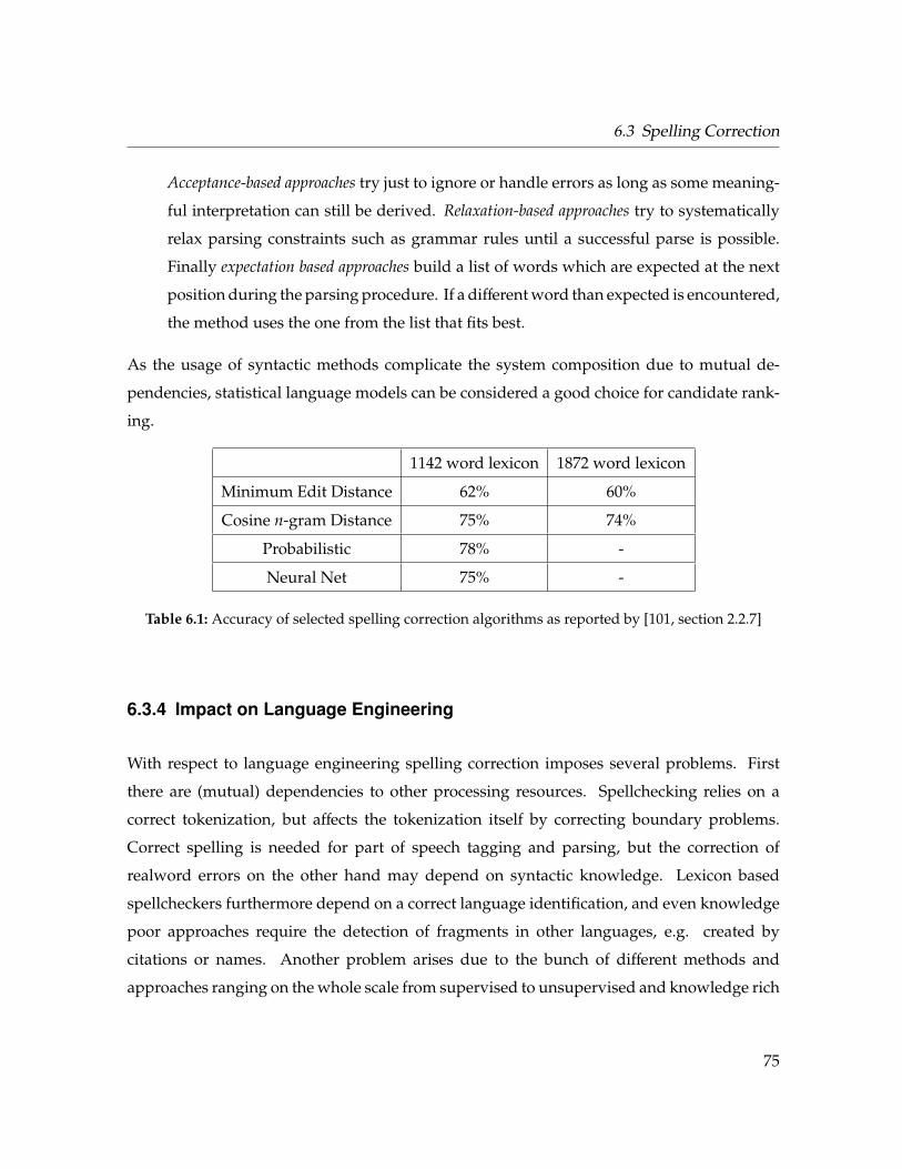
6.3 Spelling Correction
Acceptance-based approaches try just to ignore or handle errors as long as some meaning-
ful interpretation can still be derived. Relaxation-based approaches try to systematically
relax parsing constraints such as grammar rules until a successful parse is possible.
Finally expectation based approaches build a list of words which are expected at the next
position during the parsing procedure. If a different word than expected is encountered,
the method uses the one from the list that fits best.
As the usage of syntactic methods complicate the system composition due to mutual de-
pendencies, statistical language models can be considered a good choice for candidate rank-
ing.
1142 word lexicon 1872 word lexicon
Minimum Edit Distance 62% 60%
Cosine n-gram Distance 75% 74%
Probabilistic 78% -
Neural Net 75% -
Table 6.1: Accuracy of selected spelling correction algorithms as reported by [101, section 2.2.7]
6.3.4 Impact on Language Engineering
With respect to language engineering spelling correction imposes several problems. First
there are (mutual) dependencies to other processing resources. Spellchecking relies on a
correct tokenization, but affects the tokenization itself by correcting boundary problems.
Correct spelling is needed for part of speech tagging and parsing, but the correction of
realword errors on the other hand may depend on syntactic knowledge. Lexicon based
spellcheckers furthermore depend on a correct language identification, and even knowledge
poor approaches require the detection of fragments in other languages, e.g. created by
citations or names. Another problem arises due to the bunch of different methods and
approaches ranging on the whole scale from supervised to unsupervised and knowledge rich
75
6 Processing Resources
to knowledge poor. Joined with the finding that spelling errors depend strongly on the data
entry mode (OCR, keyboard, speech recognition), application context (writer’s background)
and date of study (recent texts have less nonword errors due to spellcheckers in office suites)
it is clear that there is no general solution to spellchecking.
Lexicon based methods pose a great amount of manual work for creation and maintenance,
are hard to adapt to other domains, are inferior at correcting realword errors but proved to
be successful in real-world applications — however only in conjunction with an interactive
usage. Automatic spelling correction on the other hand poses distinct constraints. Accuracy
of the best rated candidate must be high, and the erroneous correction of valid words must
be avoided by all means. Regarding the fact that spelling errors are rare, every spellchecker
working with even 95% accuracy in error detection may change more valid words to incorrect
ones than vice versa. The selection of a spellchecker relies therefore heavily on a prior
error analysis. Being confronted with a high spelling accuracy of the input the usage of an
automated spellchecker should be carefully evaluated and perhaps avoided. A high amount
of realword errors is currently best solved without a lexicon — especially in restricted domain
language.
Considering the dependencies to other modules it is suggested to always use an at least
sentence based language identification step (see section 6.1) before spellchecking. Boundary
errors are better solved in the spelling corrector than in the tokenizer and should therefore
be done by the spelling module. It may be advantageous to substitute the candidate ranking
module with a general purpose module to calculate sentence probabilities for the current
language. This module can replace the ranking of tokenizations for Asian languages as
well, and is even required for spellchecking if multi-error sentences are given. Having
three erroneous words in one sentence with three candidate corrections each leads to nine
possible sentences, thereby demanding the evaluation of every possibility. An infrastructural
requirement of spellchecking is consequently the creation of alternative annotations, which
are weighted according to a confidence measure. A feature like this would also allow to
handle realword errors, which can only be resolved via syntactic means. As well regarding
the architecture as the performance it is critical to include part of speech tagging or parsing
76
6.4 Part of Speech Tagging
as early as in the spellchecker if it is a necessary step later on. In this case, alternative
annotations should be created which can be resolved later in the workflow. Although all
current frameworks allow this, it is not a built-in feature. Annotation alternatives supported
by the architecture would allow modules to transparently get the highest ranked annotation
and ask for alternative interpretations on demand.
6.4 Part of Speech Tagging
Part of speech tagging denotes the task to assign each word in a sentence its appropriate
syntactic part of speech (see [112, chapter 10]). Those tags can be used as input for (shallow)
parsing, for filters used in terminology extraction or as input to machine learning algorithms
by providing an abstraction from the tokens.
Although a large part of words in a language may occur with several different parts of speech,
there is usually a predominant tag, leading to high baseline accuracies by just assigning every
token its most frequent part of speech (cp. [112, chapter 10 ff.]). More sophisticated state of
the art taggers reach accuracies around 95% to 97% on a token level. Although this seems to
be rather impressive, one has to be aware that this may still mean an average of one error per
sentence, assuming a sentence lengths of 20 tokens. If the tags are used as input for a parser,
this can decrease parse accuracy for sentences considerably.
In principle tagging can be seen as a straightforward task with respect to this work, as
machine learning algorithms like SVMs, naive Bayes or decision trees (see chapter 5) can be
directly employed. Input features are found in the word itself as well as adjacent words with
their affixes or part of speech tags. This may however lead to tagging every word with its
most probable tag, thereby deriving a syntactically inferior tag sequence for the sentence as
a whole. Most approaches avoid this flaw by maximizing the probability of the tag sequence
as a whole:
argmaxt1...tn
P(t1 . . . tn|w1, . . . ,wn) (6.4)
77
6 Processing Resources
A very widespread approach to determine this tag sequence is the usage of (second order)
Hidden Markov Models (see [29]):
argmaxt1...tT
T∏i=1
P(ti|ti−1, ti−2)P(wi|ti)
P(tT+1|tT) (6.5)
t−1, t0 and tT+1 are special markers for sequence start and sequence end. Transition and output
probabilities are directly estimated from the training corpus, data sparseness problems are
avoided by smoothing techniques (see section 7.2). The sequence of tags with the highest
probability is then found by using for example the Viterbi algorithm (see [131, chapter 16.3.4]).
A part of speech tagger like this is described in [29] and achieves between 96% and 97% for
English (Wall Street Journal) as well as German (NEGRA corpus). Weaknesses and properties
of this and similar approaches are found in data sparseness, size of parameter space, tagging
direction and the handling of unknown words. Although data may be sparse (which can be
handled partially by smoothing), the parameter space of trigrams is still large, and Markov
Models of higher order than two are complicated to handle. An interesting solution to
smoothing for part of speech tagging is found in [144] and uses decision trees to determine
reliable estimates for transition probabilities. The work reports an accuracy of 96.3% on the
Wall Street Journal corpus. The tagging direction determines if the probability of a tag is
derived by its preceding tags, or its succeeding tags. Although most approaches rely on
the preceding tags, there is evidence that the tags to the right are equally important. By
incorporating both preceding and succeeding tags as well as surrounding words in a Cyclic
Dependency Network, the approach presented in [158] achieves an accuracy of 97.24%. An
interesting outcome is that the symmetric usage of tag features is superior to the unidirectional
cases.
Beside the statistical approaches there are also rule-based methods available, of which the
probably best known is presented by [30]. The algorithm works by basically applying the
following steps:
1. A first training phase learns the most likely tags for every word in the first 90% of the
training data, and some baseline statistics to handle unknown words in the test data
using for example affixes and capitalizations.
78
6.4 Part of Speech Tagging
2. In a first pass all words in another 5% of the training data are assigned their most likely
tag according to the learned statistics.
3. By considering the errors in the tagged data, the algorithm successively applies rules
formed from manually defined templates, and adds the rule with the highest error
reduction to the internal rule set. Rule templates are in the form of "Change tag a to
tag b if one of the three (two, one, ...) following (preceding, ...) words is tagged z".
Input features to the algorithm are preceding and succeeding words, their tags and
capitalizations.
The last 5% of the training data are used for testing. The author notes that the amount of
rule templates cannot decrease performance, as bad templates will be outperformed and
therefore ignored. On the other hand the sheer amount of rules derived from the templates
may significantly influence runtime behavior for training, the algorithm is however reported
to be very fast in application (see [160, chapter 8.2.3.5]). The approach achieves an accuracy
of ca. 95% on the Brown corpus (see [30]). Although a comparison to other taggers is hard
due to different test data, the rule based tagger performs surprisingly well with respect to
its simple approach. Interesting again is that the tagger incorporates tags from preceding as
well as succeeding words. The approach is furthermore easy to understand, interpret and
maintain by humans, and is highly portable to other domains and languages (if the capital-
ization feature is used with care).
Besides the approaches mentioned before there are also other works using all kinds of ma-
chine learning algorithms as presented in chapter 5. [143] presents an approach using a
multilayer perceptron with recurrency to model the sequential nature of the data. The input
layer takes all of the information about preceding and succeeding tags and the output layer
represents the probabilities of the different tags. The work reports an accuracy of 96.22%
on the Penn-Treebank corpus, a robust behavior for small amounts of training data and the
shortcoming of a low processing speed compared to trigram-based methods. A method
based on SVMs is presented in [60] and achieves an accuracy of 97.16% on Wall Street Journal
data. Features used for learning include preceding words and tags, succeeding words and
79
6 Processing Resources
their possible tags, affixes, punctuation and even word length. A nice capability allows the
change of the model direction from right to left. Although the results are promising, the
authors report that the tagger is several times slower than the HMM based tagger described
above. Another approach which is based on Maximum Entropy models (see [159]) achieves
an accuracy of 96.86% on the Penn Treebank and introduces some interesting ideas. Handling
of unknown words is improved by adding capitalization features (whole word, uppercase
letter inside words etc.), ambiguities between different verb tags are decreased by searching
for specific keywords (like to, have, be, modal verbs etc.) up to eight words backwards in the
text. Tagging performance of particles is increased by enriching the model with additional
information about relations between verbs and their frequently used particles etc.
Besides supervised approaches there are also unsupervised methods worth mentioning.
An early unsupervised method is described by [150]. The basic approach is as fol-
lows:
1. Context vectors to the left and to the right are calculated for every word in the training
data. The vectors are formed by using the most frequent 250 words in the corpus with
their frequencies in the left (and right) context. Depending on the specific algorithm
those context vectors may be combined or treated separately.
2. Dimensionality reduction of the context vectors.
3. Clustering of words with respect to their context vectors (using cosine similarity and
Buckshot clustering in [150]). More sophisticated algorithms integrate the context
vectors of adjacent words or precluster the context words and then integrate their
cluster label into the context of the target word. This reflects the idea of not using the
words themselves in the context vector, but rather their anticipated syntactic behavior.
4. The tagging process assigns to every word the id of the cluster which mean is closest
to its own context vectors.
Although this algorithm does not achieve high accuracy yet and the resulting tags do not
directly map to the regular syntactic classes, it does provide unsupervised means for part
80
6.4 Part of Speech Tagging
of speech tagging. A more sophisticated approach is presented in [17] using efficient graph
clustering and co-occurrence significances. Some practical works (see [81]) give rise to the
assumption that such an unsupervised approach may even be sufficient for relation extrac-
tion tasks, despite the lack of human interpretability and inferior accuracy. A good overview
over different tagging approaches and their advantages and shortcomings can be found in
[112, chapter 10 ff.].
A general problem of all methods mentioned here is the handling of unknown words, which
were not observed in the training data. As most algorithms include the probability P(t|w) (or
P(w|t)) in some way, this value is for unobserved words determined by affixes (capitalization
etc.) from the training data. Wide-spread methods are based on the solution described by
[47]. Suffix-tries are build for a parameterized length n and a probability vector for possible
tags is assigned to every leaf. A more sophisticated method is described in [144] and starts
with a longer suffix length n which is later on pruned by calculating the information gain for
all leafs.
With respect to the presented algorithms it has to be stated that best results are given by
the tagger using the Cyclic Dependency Network (see [158]), which is very popular in ap-
plications and research. The different approaches are however hard to compare, even when
evaluated on the same data. The algorithm that shows the best practical overall properties
is given by the rule-based solution by [30], which combines fair results with high portability,
maintainability, interpretability, simplicity and a fast runtime. Furthermore the parameter
space is small, which also decreases model size significantly. In general it has to be stated that
best results are achieved by integrating context to both sides and word based features instead
of just tag sequences (cp. [158]). The inclusion of selected marker words or tags (like modals,
auxiliary verbs etc.) in a larger context may give additional insight. As some works imply,
the accuracy of state of the art approaches reached their limit, being bounded by errors in the
training data and artifacts like named entities and foreign language tokens. In fact it seems
that for most applications the choice of algorithm is less important with respect to accuracy
than the right integration and handling of unknown words, names and noise (cp. [158]).
Regarding language engineering and infrastructure, part of speech tagging reveals several
81
6 Processing Resources
implications. On the one hand, the correct integration with the tokenizer is absolutely neces-
sary. If the tagger was trained on data tokenized differently than the real data, this may lead
to small but painful deficiencies, especially with regard to unconventional corpora as given
by domain language. This demands aggregated workflow definitions, which are in today’s
architectures only available on an API level, if at all. A formal and standardized specification
is not yet possible.
Furthermore already detected numbers must be handled, which are identified in separate
modules. A part of speech tagger should in general be able to reuse existing information
about names, numbers, foreign language tokens and artifacts — in the application as well
as in the training. The inclusion of named entities causes mutual dependencies with named
entity detectors, which can be resolved by including a baseline name extractor before part of
speech tagging.
Furthermore a part of speech tagger needs access to fullform lexica with frequencies, affix
tries, if available, and depending on the specific algorithm also n-gram language models.
As all of these language resources are used broadly by language processing modules, a part
of speech tagger needs to define standardized interfaces to the resources and their access
structures. Unfortunately all currently available libraries free for research fail in at least one
or two of these demands by having named entity taggers, tokenizer, number detectors and
required resources often built in, potentially in proprietary formats. This makes the integra-
tion of existing libraries impossible, introduces error sources and decreases system runtime.
With respect to annotation type systems it is recommended to model part of speech tags as
separate annotations (instead of modeling them as features of tokens), to be independent of
the used tokenizer, which facilitates modularity and allows tags assigned to token sequences
(e.g. compounds). Another advantage given by separate annotations is the possibility of
defining alternative annotations for tags with different probabilities. Although these could
also be encoded as features, the feature-based approach is more heavy-weight and requires
subsequent modules to know about the encoding. If represented by independent annotations
it is easier to filter unwanted annotations, or to make the one with the highest probability
visible to succeeding modules which can not incorporate alternative tagging variants.
82
6.5 Parsing
It is finally suggested to always include a basic tagset in addition to the detailed one.
Some algorithms do not use the degree of detail provided my many tagsets and a map-
ping across languages is also easier (see section 8.1). This again profits from alternative
annotations.
6.5 Parsing
When handling text it is obvious that words do not occur in arbitrary order, but rather are
arranged according to a given word order. This order is implied in a hierarchical way by
grouping words into phrases and constituents like noun phrases or verb phrases, which can
then be combined respectively. The study of these regularities and constraints on word order
is called Syntax (see [112, chapter 3.2 ff.]), and the retrieval of the underlying syntax of a
sentence is normally done using grammars and parsers. As this needs a deep linguistic un-
derstanding it will only be briefly sketched to the extent necessary for language engineering
according to [112, chapter 3.2 ff. and chapter 11 ff.].
The most basic approach to define a grammar is by means of rewrite rules, which maps one
word category to several word categories (category→ category*). This means that the given
sequence on the right hand side can be replaced by the category on the left hand side. One
example of such a rule would be S→NP VB, stating that a sentence can be made up of a noun
phrase followed by a verb phrase. If the set of rewrite rules also contains words with their
categories (NN → chair) not even a separate part of speech tagger is needed anymore. This
kind of phrase structure grammar is referred to as context-free grammar, as it does not consider
the context to the right or left side of the replaced categories. The iterative application of
these rules leads to a syntax or parse tree of the given sentence, with the originating words as
terminals, and the other nodes as non-terminals. An algorithm for parsing sentences accord-
ing to a given context free grammar in its Chomsky Normal Form (CNF) is given by the CYK
algorithm ([90, chapter 3.4.3 f.]). The algorithm is complete by finding all parses sanctioned
by the rules, and has a polynomial time complexity of O(n3, |G|) with n being the amount of
tokens in the sentence and |G| denoting the size of the grammar.
83
6 Processing Resources
One widespread extension to context free grammars is the introduction of probabilities for the
rules of the grammar, leading to a probabilistic context free grammar (PCFG). PCFGs are con-
sidered to be "the simplest and most natural probabilistic model for tree structures" (cp. [112,
chapter 11]) with well understood theoretical base and algorithms. These grammars have sev-
eral interesting properties, as described in [112, chapter 11.1]:
1. As sentences tend to have many structurally different but yet valid parses, a PCFG can
give some ideas about which parse may be the most probable one and also provides an
ordering. The probability is however hard to interpret directly.
2. PCFGs are robust by being able to also cover grammatical mistakes and disfluencies by
including low probability rules for such constructs instead of just rejecting them.
3. Some biases are introduced by PCFGs, like assigning greater probabilities to smaller
trees.
4. Due to the context-free nature of the grammar, PCFGS have also structural deficiencies.
The probability of a noun phrase to expand in a certain way is for example independent
of the following or preceding verb phrase, which is clearly insufficient.
5. If the grammar acts in a non-lexicalized way being only based on word categories,
the expansion of for example a verb phrase to a verb prior to two noun phrases is
independent of the verb itself. This is incorrect as this is more likely the case with
ditransitive verbs like tell (see [112, chapter 12.1.4]). Lexicalized extensions to the
regular PCFG can be used to deal with this problem.
Furthermore a PCFG can be considered a probabilistic language model, which is however
inferior to a n-gram model with n > 1 as context is not taken into account. Probabilities of
a string can be calculated by the inside algorithm or the outside algorithm, and the most
likely parse for a sentence can be determined by a Viterbi-style method (see [112, chapter
11.3 ff.] for more details). Interestingly the probabilities or even the whole grammar can be
induced by given treebanks. Evaluation of parse trees is normally done by comparing the
84
6.5 Parsing
output of the parser to gold standard trees using the PARSEVAL method (see [5]). Every
tree is considered a set of non-terminal nodes with their boundaries and labels, allowing to
use standard precision and recall measures for evaluation. Precision is the ratio of correct
elements in the set (correctly identified non-terminals with correct boundaries), and recall
states the fraction of correct elements from the gold standard retrieved by the parser. The
start node may be excluded, as it is always right (at least with respect to its boundaries), and
pre-terminals may be excluded as they would merely express the result of the part of speech
tagging step — even if the tagging is done as part of the parsing procedure. Although the
PARSEVAL method is widely used, it is criticized for scoring even baseline methods high and
for not suiting the nature of the Penn treebank (flat trees, no disambiguation of compound
noun structures etc.), which is widely used for parser evaluation and induction (see [35],
[112, chapter 12.1.8]).
Besides the parsers that were built using phrase structure grammars, there is another
widespread approach to parsing which directly derives the relations between the head of a
phrase (e.g. the noun) and its dependents (e.g. the adjectives describing the noun). These
dependency grammars (see [157]) are built on the assumption that every sentence contains
one head, of which all the other words are dependents, or else depend on another word
which itself leads to the headword. While parsing results of a phrase structure grammar
are depicted as trees, dependency grammars are visualized by curved arrows, showing
the pairwise relations between the head and its dependents (see [112, chapter 12.1.7]). The
definition of such a grammar involves the definition of a lexicon, which categorizes each
word for category, gender, number and the arguments it takes (as subject, object etc.). A
dependency grammar is especially useful with respect to languages with free word order,
such as Czech and Turkish.
Regular approaches to parsing which are providing grammars, lexica or annotated treebanks
are of minor interest to this work of language engineering. This is due to the fact that
the construction of these resources is even for trained linguists time consuming as well as
complicated and cannot be performed easily. Therefore a language engineer always depends
on existing and pretrained libraries, which limits the reuse in a modular system for different
85
6 Processing Resources
domains massively. And even if treebanks and grammars can be provided, it needs to be
stated that the best parsers available today do not exceed a precision or recall above 90%
(see [112, chapter 12.2.4]) — and even these results are only reached for text of good quality
provided by the Penn treebank.
To deal with these problems there are also several approaches for unsupervised parsing
available, providing means to extract syntactic structure even from domain language with-
out the need for annotated corpora or the definition of a grammar. A straightforward and
appealing approach using co-occurrences called UnsuParse is described in [80] and [78] and
follows these basic steps:
1. A separation value between two adjacent words w1 and w2 is defined using co-
occurrence significances between the words, sentence start marker (denoted by ˆ) and
sentence end marker (denoted by $).
sep(w1, w2) =sig(w1, $)sig(ˆ, w2)
sig(w1, w2)2 (6.6)
A separation value larger than 1 can be seen as indication for a constituent border
between the words, as they rather occur at start and end of constituents than adjacent
to each other.
2. The separation values are calculated for every adjacent pair of words in the corpus.
3. The algorithm iteratively merges the pair of words with smallest separation value to be
a new constituent. If one of the words is already grouped, its according constituent is
nested instead.
Extensions to the basic algorithm can be found in using part of speech tags to avoid data
sparseness, including a larger range in separation calculation and using constituent fre-
quency as an additional filter criteria besides co-occurrence significance (see [80]). Although
the results of the algorithm are inferior to supervised methods, it still provides a PARSEVAL
F-measure of 69.5% for German (71.8% for English) by using manually annotated part of
86
6.5 Parsing
speech tags, and 61.7% on unsupervised tags provided by UnsuPos (see [17]) on the NEGRA
corpus for sentences with a maximum length of 10 words (see [79]). Besides unsupervised
methods for phrase structure grammars there are also unsupervised dependency grammar
parsers available (e.g. [152]).
With respect to language engineering it has to be stated that all methods based on manually
annotated treebanks or manually created grammars have a very high initial effort to be fitted
to a domain and cannot easily be adapted to other domains. Robustness is especially high
for probabilistic methods, but even the best methods on high quality corpora are still error
prone. Unsupervised methods promise portability, adaptability and ease of use for the price
of furthermore decreased precision and recall — which might on the other hand still be
sufficient for many information extraction tasks, as for example seen in [81]. The statistics
given in chapter 4 can give a first feeling for the method to be used, especially in comparison
to texts used for training of prepackaged parsers (e.g. the Penn treebank). Domain texts
which vary strongly in syntax, morphology and terminology may better be processed with
unsupervised methods, as individual training is normally not feasible, and the application
of pretrained parsers on such corpora may have even stronger drawbacks then using unsu-
pervised methods. If in doubt, a small amount of sentences can be parsed and manually
evaluated, although even this requires a good linguistic understanding.
Annotation models for parsing can be designed in several ways having different levels of
encapsulation. One way is the definition of a single annotation for the whole sentence, con-
taining the complete parse tree as a feature. Although this seems straightforward, it hinders
reusability and modularity. Syntactic annotation can be seen as having several levels — the
one with the word categories (part of speech tags), the ones with phrases and the root of the
tree. Interestingly all these levels can be created and used independently of each other. While
a part of speech tagger can be employed for the first level, a chunk parser is used to find
phrases and the complete parse tree can be created by a PCFG parser. Usage for information
extraction is also manifold, as many methods only need part of speech tags, and others rely
merely on chunks and phrases. Therefore all nodes of a parse tree (as well terminals as
non-terminals) should be encoded as stand-alone annotations, which refer to their parent (or
87
6 Processing Resources
children respectively). This also enables a parser to use preexisting part of speech tags or even
phrase annotations created by other modules — therefore fostering reusability, modularity
and maintenance. Another question would be, if the part of speech tags may be encoded
within token annotations, or if the root node of the parse tree can be specified in the sentence
annotation. This can be seen as a tight coupling of different modules and should be avoided.
Not only that the parser needs to be aware of the internal structure of those annotations,
following modules would be dependent on two preceding modules, where one might have
been sufficient.
With respect to requirements to language engineering architectures, parsing benefits from
the availability of alternative annotations. Although parsing can use this feature directly in
the form of alternative parse trees with different probabilities, it is also a central module in
resolving earlier variations. Correction suggestions from a spellchecker can be reweighted
or filtered by a parser as described in section 6.3 and [101, section 3.2 ff], alternative part
of speech tags can also be resolved by similar means. Information extraction algorithms on
the other hand may profit from the definition of different parse trees with distinct probabili-
ties.
6.6 Information Extraction
Between simple keyword based methods and the extremely ambitious field of a complete
language understanding, a new field called Information Extraction (IE) gained a lot of scientific
interest in the past two decades. Focused on extracting only specific facts and the relations
between them, this task is manageable as well as sufficient for many applications.
The field of information extraction especially gained attention during the seven Message
Understanding Conferences (MUCs) initiated by the Defense Advanced Research Projects Agency
(DARPA), which were held between 1987 an 1998 (see for example [90, chapter 3.1], [64] or
[67]). The initiative had a very positive influence on the scientific community by posing a
competitive challenge on real data and providing preannotated training and test data. After
having focused on naval operation messages first, MUC-3 and MUC-4 gained more interest
88
6.6 Information Extraction
with the task of event extraction from news corpora, in particular the detection of terrorist
attacks. MUC-5 introduced a more business related goal with the extraction of joint venture
announcements. MUC-6 was the first conference to treat Named Entity Recognition (NER) as
an independent subtask, thereby acknowledging its importance to the field of information
extraction. Named Entities in the sense of the MUCs are proper names of people, companies,
places and numbers like date, time, money or percent values (see [27]). Relation Extraction
in the MUCs was oriented towards filling the slots of given templates, thereby often called
template filling.
The two following (and closely related) subsections will describe processing resources for
Named Entity Recognition and Relation Extraction.
6.6.1 Named Entity Recognition
Advanced information extraction and relation extraction methods depend on the detection
of their basic components. These atomic pieces of information, often enough given by just
one or two (adjacent) tokens, are with respect to most applications proper names denoting for
example people or places. Influenced by the tasks of the Message Understanding Conferences
5 and 6 the greatest part of the scientific community tests their Named Entity Recognition
systems on these proper nouns and numeric expressions like money or date values. This
work will however focus on (named) entities. Regarding the engineering of information
extraction systems, numeric expressions are usually handled in separate modules, as their
recognition is far easier and needs to happen in an early stage, therefore easing the tasks of
e.g. sentence boundary detection or part of speech tagging. On the other hand, the pure
detection and categorization of proper nouns seems to be insufficient, as information facts
of interest may include actions or properties expressed by noun phrases or modifiers like
adjectives or adverbs. Some domains are however also interested in mixed names containing
characters as well as digits (e.g. protein names in biomedicine).
Named Entity Recognition can be divided into two different subtasks, entity detection and
entity classification (cp. [98]). While both can be considered classification problems for
89
6 Processing Resources
machine learning algorithms as presented in chapter 5, the first step is often achieved by
simpler means, like filtering for the right part of speech tag, or is even omitted by just
classifying every word’s category. While all machine learning algorithms are in fact applicable
to the problem (although with different success), it must be stated that the choice of features
is at least as important as the choice of the method to use (see [124]).
For several years, rule based methods achieved superior results than machine learning based
techniques (see [175]), until those yielded similar results in MUC-6 and MUC-7 (cp. [38]).
But even in MUC-7 five out of eight systems were still rule-based, and they are considered
to be a preferred technique if labeled data is not available (see [124]). The best known rule
based system is probably FASTUS (see [12], [13]), which is based on a series of finite-state
transducers and achieved in MUC-6 an F-measure of 94%. Besides the good performance the
system also has a fast runtime (cp. [12]). Other rule-based systems are for example Proteus
(see [66]), 59% precision and 32% F-measure in MUC-5) and the domain specific ProMiner
(see [72]) which achieved ca. 80% F-measure for fly and mouse related entities, and 90% for
yeast.
Support Vector Machines (see section 5.2) were applied for example in [93] or [89]. Especially
[93] is interesting here, as it is dealing with domain language from biomedicine. For the task
of detecting proteins, DNA types and other biomedical entities, an SVM with polynomial
kernel is trained on feature vectors (words, pre- and suffixes, part of speech tags, etc.) which
were enriched with state sequences of an HMM model. Classification is done word-wise,
and every word is labeled according to if it is the start token, the end token or an intermediate
token of one of the target categories. This way of classification is also used in other works
(e.g. [27] or [38]), and avoids the complexity of checking every multiword combination of up
to n words (although one needs to eliminate impossible sequences afterwards). This method
achieves an F-measure of 73.6% on the biomedical data (see [93]). A decision tree based
method is for example presented in [126] and reaches on MUC-6 data precision and recall
values of ca. 80% for organizations and ca. 90% for persons. The method uses C4.5 trees on
simple features of dictionary and part of speech tags with different levels of pruning.
There is also some work using Maximum Entropy models as for example presented in [38]
90
6.6 Information Extraction
or [27]. [27] uses binary features for capitalization (initial, all), lexicon features (build from
all words with a frequency > 2), features based on dictionaries (names, locations etc.) and
the input of other NER systems like Proteus. The system achieves an F-measure of 97.12% on
data from MUC-7 (see [27]). Furthermore the system is described as portable and frugal with
respect to training data. The Menergi system presented in [38] follows the same approach
and shows an error reduction of 27% for MUC-6 and 14% for MUC-7 data by incorporating
global features. These are related to other occurrences of the same word in for example an
unambiguous context or as an acronym.
A common base for successful NER systems is either the usage of manually created rules
(e.g. [12]), manually created dictionaries (e.g. [27]) or manually labeled training data (as e.g.
provided my the MUC conferences). This poses a problem for porting the systems to other
domains and languages, as very often none of the above is available. Besides the selection of
features, the quality, extent and usage of these resources influence named entity recognition
massively (see e.g. the different results for English and German in [116]). With respect to
language engineering it is to state that the choice of method is truly secondary to the design
of the overall NER system. To keep the amount of manually created resources down, several
researchers (e.g. [31] or [7]) proposed so-called bootstrapping methods, which can be trained
iteratively. Bootstrapping algorithms can be seen as iterative supervised classifiers, which
are initially trained on a very small training set consisting of several examples, which is
called seed SSeed. After application of the classifier and an additional evaluation and filtering
step of the results SNew, which leads to S′New, the classifier is trained on the merged set of
SSeed and S′New. Nearly all kinds of supervised classifiers can be integrated into a semi-
supervised bootstrapping algorithm, although the original approach uses extraction patterns
(see [135, 136]), for example with regular expressions:
1. Define the small training set SSeed of labeled entities.
2. Search and annotate the elements of SSeed in the document collection D and extract
features from their context according to a specified window size. Every occurrence of
an entity in a document leads to one or more context feature vectors.
91
6 Processing Resources
3. Build extraction patterns P from the set of feature vectors.
4. Generalize extraction patterns to avoid overlearning.
5. Apply the extraction patterns on the document collection D, to extract new entities.
6. Weight the entities SNew and the patterns P using external or internal knowledge, or
even manually. Then filter the entities and patterns according to given thresholds.
7. Set SSeed = SSeed⋃
S′New, and start the process iteratively again.
8. Stop the process after the execution of N iterations, after reaching convergence or on
the fulfillment of other conditions.
To ensure a high quality of tuples and patterns and convergence of the algorithm, it is
important to implement confidence measures and to delete elements which do not fulfill
certain thresholds. A widespread measure was defined by [136] and is based on extraction
frequencies of patterns and tuples (see section 10.9).
Bootstrapping methods gained a lot of attention, as they avoid the time consuming manual
creation of resources and recent work shows that they even rival baseline supervised methods
(see [40] or [125]).
As mentioned before, the choice of features massively influences NER performance. Possible
features are for example (cp. [124]):
1. The case of a word, including initial cap, all characters are capitalized, mixed capital-
ization etc.
2. If a word contains, starts or ends with punctuation marks, apostrophes, hyphens or
ampersands.
3. If a word is made up of digits, contains digits or matches specific digit patterns.
4. The morphology of a word as well as prefixes, suffixes, stems and lemmas.
5. Part of speech of a word.
92
6.6 Information Extraction
6. Nominal attributes like a lowercase version of a word.
7. Numerical attributes like the length of a word.
8. Lexicon features, like a vector with the length of the general lexicon, and the index of
the given word is set to 1.
9. Parsing features, like head and governor of noun phrases.
10. External features, like for example derived from exhaustive web corpora.
11. WordNet based features like sub- or supertypes, subparts or cohyponyms. Even se-
mantic distances based on WordNet distances are possible.
12. List lookup features, like if a word is contained in a location dictionary (perhaps with
an associated probability), or if the word is frequently part of the NEs in question. List
lookups can also be performed softly, e.g. by looking up the stem or lemma, a Soundex
code or similar words (for example using the Levenshtein distance).
13. Global features like previous occurrences of a word (and perhaps its classification there),
anaphoras, local syntax (enumerations, title etc.), meta information (HTML header etc.)
or co-occurrences.
Examples of such feature lists can be found in most NER publications, like in [40], [27], [38]
or [49].
From the language engineering point of view, NER is interesting because of its mutual de-
pendencies. Spelling correction (see section 6.3) and part of speech tagging both have issues
with out-of-vocabulary words as given by named entities (see [101, section 1.3] and [158]).
The recognition of entities on the other hand relies heavily on features based on (correctly
spelled) words and their part of speech tags. Also language identification may suffer from
high ratios of names, as they are likely to origin from foreign languages (e.g. English com-
pany names in German text). Regarding the fact that state-of-the-art spellcheckers and part
of speech taggers integrate simple named entity recognizers, it can be assumed that these
93
6 Processing Resources
ties can be solved best by integrating two NER modules into the system: A simple baseline
method (e.g. [119, section 3.1]) and the real NER module. Iterative approaches to the problem
are also possible (see section 8.2), but demand much higher computational requirements and
architectures offering enhanced workflow definitions.
Regarding portability and initial effort to establish NER systems, it is to mention that manually
annotated texts or handcrafted resources are absolutely necessary, which reduces reusability
on different corpora significantly. As completely unsupervised approaches do not perform
well enough, bootstrapping methods should always be applied when engineering NER
modules. Although current bootstrapping methods do not reach the performance of better
supervised systems yet, they still provide fast and efficient means to reduce the manual effort.
Even the creation of some regular expressions to create initial dictionaries is a huge relief in
engineering.
Named entity recognition is interesting with respect to the language engineering architecture.
Although the annotation model is pretty straightforward (direct annotation of found entities
with a specific NE type), the requirements to workflow control are clearly more demanding.
As recognizers often rely on dictionaries, which contents need to be matched in the text, the
tokenization of the dictionary data needs to be in concordance to the general tokenization
step. If this is not already done in a separate Gazetteer module (which just moves the prob-
lem), the named entity recognizer needs to call the tokenizer as part of its own initialization
process — and therefore needs nested workflow definitions. As current systems further-
more should integrate bootstrapping methods, iterative processing of the whole collection is
necessary, therefore demanding cascading workflows. As well nested as iterative workflow
definitions are not possible in today’s architectures without direct API access (see chapter
3).
6.6.2 Relation Extraction
Relation Extraction from text is concerned with detecting and isolating n-tuples of terms
which present an instance of a given semantic relation. By being assigned the task to engineer
94
6.6 Information Extraction
a relation extraction system, it however becomes evident that the necessary approach varies
massively depending on the type and arity of the relation and the involved entities. While a
semantic relation may in fact be rather arbitrary, the scientific work concentrates on linguistic
relations and logical relations.
A simple form of semantic relationship between terms is given by those relations which
form the base of a thesauri (see section 7.3). Besides synonymy or antonymy there are also
hyponymy (subtype and supertype), meronymy (part to the whole) and co-hyponymy (subtypes
of same supertype) of interest. While synonymy and antonymy may occur in all open-
class part of speeches, the other relations are merely considered for nouns. Approaches
to detect these kinds of relations are used to construct thesauri or ease their maintenance,
and either use corpus statistics or simple pattern matching methods. The usage of patterns
is for example described in [73] and is based on lexico-syntactic patterns like such NP as
NP,*(and|or)NP to extract hyponymy relations. For a set of 152 instances extracted from
a 8.6M token encyclopedia corpus, 61 relations could be verified using WordNet — and
even more might have been right. The authors report that the approach did not work well
for meronymy relations. A good example for methods based on corpus statistics is given
in [19] (and [110, chapter 2.1 and 4]) and uses co-occurrences (see section 7.1) of higher
order:
1. Calculation of co-occurrences on the given corpus
2. Creation of co-occurrence sets consisting of a word with all its significant co-occurrences
3. These sets are treated as sentences of a new corpus and are origin for the calculation of
co-occurrences of the second order etc.
The method aims at creating groups representing specific meanings. Words which for exam-
ple co-occur on the second level, are part of similar contexts in the first level. The authors
describe that the semantic purity of the co-occurrence groups increases with higher levels,
and that the groups contain high ratios of co-hyponyms, synonyms and hyponyms. It is
however still hard to separate the instances of these relations. Besides co-occurrence based
95
6 Processing Resources
methods (see also [15] for synonym detection or [149] for semantic similarity) there are also
graph based methods available (like e.g. given in [23]), but nearly all methods are using some
kind of contextual similarity of words. Unfortunately no method reaches sufficient quality
for automatic usage and therefore need manual correction. Other kinds of linguistic relations
which are useful for relation extraction methods are given by direct syntactic dependencies
as for example between a head and its modifiers. As these relations are directly given by a
parse tree (see section 6.5) they will be omitted here.
Logical relations are given by higher order semantics and denote relations between abstract
concepts in the real world. Examples for these meaningful connections are given by com-
panies and the location they are based (see [42]), authors and titles of their books (see [31])
or merging companies (see [172]). Relations like this were defined and used in the Message
Understanding Conferences and are frequently reconsidered in works on relation extraction.
Methods used in logical relation extraction are based on Named Entity Recognition (to eas-
ily identify candidate tupels) and use similar means. Machine learning approaches rely on
annotated training data, and learn from contexts to classify new candidates. A predominant
machine learning technique in this area is found in SVMs with specialized kernels. [42] for
example presents a method using SVMs which incorporate a kernel over dependency trees
enriched with additional word features such as part of speech, wordnet relations and entity
types. Goal is the extraction of 24 relation types (e.g. based-in, Founder, Subsidiary) between 5
types of entities (Person, Organization, Facility etc.). Performance of the system is measured on
the 5 high-level relation types, and achieves up to 45.8% F-measure on the Automatic Con-
tent Extraction (ACE) corpus which is provided by the National Institute for Standards and
Technology (NIST). A good overview over different kernel methods for relation extraction is
given in [173], which tries to detect the relations person-affiliation and organization-location on
200 newspaper articles. Best results (F-measures of 86.8% for person-affiliation and 83.3% for
organization-location) are reported for a SVM using sparse subtree kernels.
Besides purely supervised approaches there is, similar to the field of Named Entity Recogni-
tion, much work in the area of semi-supervised methods such as bootstrapping algorithms.
One of the first systems is presented in [31], but can’t be seen as universally applicable as
96
6.6 Information Extraction
it incorporates HTML tags in learned contexts, which makes it especially easy to extract list
based information from the web. A more sophisticated approach is outlined in [7] and rep-
resents contexts in a vector space model. The system called Snowball uses a Named Entity
Recognizer to identify candidates for the Company-Location relation and builds three vectors
(left, middle, right contexts, entries are based on term frequency) for every occurrence. After
clustering the context vectors, the centroids of the clusters form the new patterns. These
patterns can then be used to extract new relation tuples. The addition of the clustering
step serves as a generalization method to avoid overfitting to training examples. Between
the iterations of the bootstrapping algorithm, patterns and tuples get weighted using spe-
cial confidence measures. The quality of tuples is based on the product of the confidence
measures for the patterns which extracted this tuple, the quality of a pattern is determined
by the ratio of correct tuples it extracted (with respect to already known facts). A detailed
overview is given in [7]. The algorithm achieves precision and recall values of over 80%
on newspaper articles (ca. 178.000 documents), if only those tuples are considered which
occur at least twice and not every occurrence needs to be found. Some basic work in the
field of bootstrapping relations and especially on confidence measures is found in the work
of Riloff (e.g. [135] or [134]). The papers describe a system called AutoSlog which was used
to extract terroristic events on MUC-4 data. Linguistic patterns like <subject><passive-verb>
are used together with trigger words (like killed or bombed for the verb) and hard and soft
constraints for the slot to fill (which would be the subject in this example). Given a training
sample the system created a dictionary of patterns which achieved ca. 98% of the result of the
same system (ca. 50% F-measure on MUC-4) using manually created rules. The first version
of the algorithm required human filtering of patterns before applying them, the following
versions used bootstrapping to remove the manual step (see [135]). [136] uses sophisticated
confidence measures like the RlogF metric. Other interesting bootstrapping approaches are
presented in [52] (bootstrapping without a seed), [154] and [155] (using semantic similarities
based on WordNet) or [171] (counter-training based on document relevance).
Relation Extraction poses no requirements to language engineering beyond basic functional-
ity. Although it depends on various other modules like tokenization, part of speech tagging,
97
6 Processing Resources
named entity recognition and even parsing, it does not introduce mutual dependencies.
The named entity recognition and extraction step might be performed as a part of relation
extraction (e.g. [31]), but a separate step for this increases robustness, portability and mod-
ularization. A deep parsing step might be omitted in favor of shallow parsing (e.g. [59]) to
reduce system complexity, however it can not be stated whether this decreases system perfor-
mance. Some works prefer dependency parsers over syntactic parsers (e.g. [58] or [164]), but
[91] indicates that their performance might be inferior. Annotations are created with the type
of the relation to be found (using annotation inheritance if possible to express sub-relations),
which point to the corresponding entity annotations. With respect to adaptability, reusability
and initial effort, pattern based bootstrapping methods seem to be the predominant choice.
They can be created fast with reasonable human effort, can be adapted to other systems
and domains easily and the resulting patterns may even be extended, adapted or main-
tained manually. Bootstrapping methods however need cascading and iterative workflows
on document and collection level, which is not directly provided by current engineering
architectures.
98
7 Language Resources
In contrast to the term Processing Resources, which refers to mainly programmatic resources,
the term Language Resources denotes resources which can be seen as data-only (see [44]).
This chapter will focus on Language Resources which are of general usage for information
extraction tasks and will introduce them with regard to Language Engineering. Language
resources which are closely related to processing resources (like trained models etc.) are
neglected here, as they were (to the extent of their relevance) discussed in the sections about
processing resources.
7.1 Collocations and Co-occurrences
Collocations and co-occurrences are a kind of language model describing the statistical signif-
icance of words occurring together in contexts. While collocations denote words occurring
right beside each other (bigrams), co-occurrence is a more flexible term, which is also used for
words occurring significantly together in larger contexts. Contexts are chosen with respect
to the application and range from bigrams over n-word windows to whole sentences or even
paragraphs.
Given the frequencies f (w1), f (w2) and f (w1w2) of two words w1 and w2 in a corpus of
size n, the corresponding probabilities are given by P(w1) =f (w1)
n , P(w2) =f (w2)
n and
P(w1w2) =f (w1w2)
n . These probabilities can be used to calculate the significance of the
joint occurrence (within a given context C) in different ways with specific characteris-
tics.
99
7 Language Resources
7.1.1 t-Score
The t-test is used for estimating the significance of co-occurrences by calculating the ratio
between the difference of observed (x) and expected mean (µ) and the variance (s2) of the
sample (cp. [112, chapter 5.3.1 ff]):
t =x − µ√
s2
n
(7.1)
To apply this test for co-occurrence calculation, the sample is the amount of all bigrams (resp.
two word combinations) in the corpora, and the expected mean and variance are derived
by the null hypothesis of assumed independence. By assuming independence the expected
mean is given by µ = P(w1)p(w2) and variance is approximately s2≈ P(w1w2) (for small
P):
t =P(w1w2) − P(w1)P(w2)√
P(w1w2)n
(7.2)
The value of t can be looked up in tables to derive the according significance level, as for
example given in [33, pg. 231]. A t-value of 2.576 corresponds to a significance of α = 0.5%.
The t-test is especially appropriate for small probabilities, but as a shortcoming is based on
the assumption of normally distributed data, which is often not the case (see [112, chapter
5.3.3]).
7.1.2 Likelihood Ratios
Likelihood ratios compare two given hypothesis by calculating a ratio of their likelihoods,
thereby stating which one is more probable to have led to the observed results. To apply
this for co-occurrences the following two hypothesis are formulated (cp [112, chapter 5.3.4
ff]):
1. The first hypothesis formalizes the independence case by stating that
P(w2|w1) = p = P(w2|¬w1) (7.3)
100
7.1 Collocations and Co-occurrences
2. The second hypothesis states the dependence of w1 and w2 by
P(w2|w1) = p1 , p2 = P(w2|¬w1) (7.4)
By assuming an underlying binomial distribution, we can calculate the probability of an
observation as follows:
b(k; n, x) =
(nk
)xk (1 − x)n − k (7.5)
Now the likelihoods of the two hypotheses can be reformulated as:
L(H1) = b( f (w1w2); f (w1), p) b( f (w2) − f (w1w2); n − f (w1), p) (7.6)
L(H2) = b( f (w1w2); f (w1), p1) b( f (w2) − f (w1w2); n − f (w1), p2) (7.7)
Normally the logarithm of the likelihood ratio is used, which is easily calculated
as:
logλ = logL(H1)L(H2)
(7.8)
The interpretation of the likelihood ratio is more convenient than for example the t-value,
which needs to be looked up in tables. Furthermore by being based on the binomial
distribution the method is more appropriate for the calculation of co-occurrences (cp.
[50]).
7.1.3 Mutual Information
The pointwise mutual information measure is calculated by the logarithm of the ratio of the
observed joint frequency and the estimated joint frequency under the independence assump-
tion:
I(w1,w2) = log2P(w1w2)
P(w1)P(w2)(7.9)
This measure can also be derived from Information Theory, thereby expressing the amount
of information provided by the occurrence of w1 about the occurrence of w2 (cp. [112, chapter
5.4 and 2.2.3]).
101
7 Language Resources
Mutual information is known to be problematic with respect to sparse data, as seldom events
(e.g. two words which occur only once in the corpus, but there together) lead to high values.
An improved measure is given by the localized mutual information which is weighted by
the joint frequency:
I(w1,w2) = P(w1w2) log2P(w1w2)
P(w1)P(w2)(7.10)
7.1.4 Co-occurrences and Language Engineering
Besides the measures presented above there are several other significance measures avail-
able with other characteristics. The main differences are the assumption of the underlying
distribution and the handling of sparse events and sparse data in general. Comprehensive
overviews are for example given in [32] or [53].
Co-occurrences are sometimes considered to be less predictive as language models based
on word n-grams (see e.g. [101, chapter 3.3]). Regarding the fact that only significant pairs
of words are calculated, they are however easier to model and to apply and demand less
memory for persistent storage than for example a comprehensive trigram based language
model.
Co-occurrence based processing resources include for example spelling correction (see
[140]), part of speech tagging (see [17]) and even unsupervised syntactic parsing (see
[80]).
7.2 Language Models
Although the term language models can and is broadly used for statistical models derived from
corpora (like for example co-occurrences or collocations) this section refers to word n-gram
based language models. In those models a large training corpora serves as a basis to calculate
frequencies of for example n = 2 (bigrams) or n = 3 (trigrams) adjacent words. Based on these
102
7.2 Language Models
frequencies f (w1 . . .wn) the according probabilities can be derived by using for example the
maximum likelihood estimation (cp. [112, chapter 6.2.1]):
PMLE(w1 . . .wn) =f (w1 . . .wn)
N(7.11)
The probabilities of the language model can be used in arbitrary ways such as Markov
Models or Bayesian methods. A frequent usage is the calculation of the probability of a given
sentence with respect to a given model. To do so, it is assumed that the occurrence of a word
is only determined by the last n− 1 words — although this is not always the case, the n− 1th
order Markov assumption (see [112, chapter 6.1.2]) is very useful for practical applications
by limiting the parameter space:
P(w1 . . .wn) =
m∏i=1
P(wi | w1, . . . ,wi−1) ≈m∏
i=1
P(wi | wi−(n−1), . . . ,wi−1) (7.12)
Unfortunately n-gram models suffer from the major drawback of data sparseness and model
size. Although models of higher n would theoretically lead to better results, the model
size grows exponentially in n and still a large amount of possible n-grams is never seen in
the training data. Therefore many n-grams are assigned zero probabilities which can lead to
undesirable results through propagation. This problem is addressed by smoothing techniques,
which try to assign small probabilities to n-grams never encountered in the training data (see
[112, chapter 6.2.1 ff]).
One popular smoothing method (also known as the adding one method) is the usage of
Laplace’s law:
PLap =f (w1 . . .wn) + 1
N + V(7.13)
V denotes the size of the (closed) vocabulary. This method can also be seen as a Bayesian
estimator which assumes a uniform prior distribution of events (see [112, chapter 6.2.2 ff]).
For large vocabularies and sparse data this method however distributes a large portion of
the probability space to unseen n-grams. For an overview of smoothing methods see [112,
chapter 6.2].
Language models are broadly used in language engineering, as for example in lan-
guage identification (section 6.1), tokenization (section 6.2) or spelling correction (section
6.3).
103
7 Language Resources
7.3 Thesauri
By building an information extraction system, there are normally two types of text of inter-
est:
1. The text which is extracted as k-tupels of multi-words (the elements of the extracted
relations)
2. The context window of text enclosing the k-tupels
For both types of text it is of great importance to integrate knowledge about synonymy,
homonymy, hyponymy and meronymy. The k-tupels which will be extracted might be input
to later Data Mining or reporting steps and therefore need to be identified reliably. It is crucial
that one entity is not listed redundantly using different lexical tokens (as would be the case
with synonyms), or two different entities are cumulated because they are expressed the same
way (as would be the case with homonyms). Using hyponymy and meronymy the extracted
facts can be cumulated for reporting and data mining, providing much more insight into
textual collections.
The same advantages apply while handling the context windows containing the k-tupels. As
most information extraction systems work with some kind of similarity measure using the
context window as a basis, it can be seen as crucial to be aware of synonyms, homonyms etc.
for the matching of patterns respectively the calculation of similarities.
While synonyms as well as ambiguous words can in principle be calculated dynamically (cp.
[166]), they can also be specified in a so-called thesaurus. A thesaurus is a knowledge base
defining a specific vocabulary and the relations between its terms for the purpose of documen-
tation. Possible relations are synonymy and hyponomy/hyperonomy between terms. Synonymy
relations define synsets of interchangeable terms, of which one is marked as the representa-
tive of the group, hyponomy/hyperonomy relations define links to narrower and broader terms.
Although the hyponomy relations lead to a hierarchical structure within terms, a thesaurus
is considered to be a graph because of the other relations and possible polyhierarchical
constructs and is therefore also called a word net.
104
7.3 Thesauri
7.3.1 WordNet
With repect to NLP there are specific linguistic thesauri which aim at defining the complete
vocabulary of a given language. The best known is probably WordNet1, which was influ-
enced by psycholinguistic theories of the human lexical memory (see [120]).
WordNet organizes the contained terms with respect to meaning rather than word forms and
structures them in five syntactic categories: Nouns, adjectives, verbs and adverbs. Function
words are omitted, assuming that these words are stored separately as syntactic components
of the language. The distinction in these five categories is due to psycholinguistic theories,
which assume that the different syntactic categories are stored differently in the human con-
scious.
WordNet is organized by the use of lexical relations between word forms and semantic re-
lations between word meanings. Synonymy and antonymy are lexical relations, which are
defined within word forms. As [120] points out, synonymy as well as antonymy are hard to
define. A common definition of synonymy is that two expressions can be substituted without
changing the meaning of a sentence. While synonyms according to this definition are very
rare, it is more applicable to define synonyms with respect to a specific linguistic context.
Two words are synonyms with respect to a given linguistic context if they are interchange-
able in this context without changing its meaning. According to the authors of WordNet,
the definition of synonymy in terms of substitutability is one reason for the partitioning of
WordNet into the different syntactic categories, as only words with the same part of speech
can be substituted by each other.
A similar problem arises with antonymy. While it seems to be convenient to define the
antonym of a word x to be not-x respectively the opposition of x in general, this definition is
often wrong. Association tests indicate that antonymy is a semantic relation between word
forms, and not between meanings. Although for example large is clearly opposed to little and
big is opposed to small, only large/small and big/little are recognized as antonyms (see [120]).
Adjectives which have no direct antonym are (if possible) linked to similar adjectives which
1http://wordnet.princeton.edu/
105
7 Language Resources
have a direct antonym. This similar relation between adjectives states a similar meaning —
although however no real synonymy.
Synonymy as well as antonymy may be defined in all the syntactic categories of WordNet,
although antonymy is mainly a matter with respect to adjectives, and real synonymy is rarely
the case with verbs, due to their slight changes in meaning with respect to different linguistic
contexts.
Two important semantic relations between word meanings in WordNet are hypon-
omy/hyperonomy and meronymy/holonymy, which are mainly applied to the category of nouns.
Using these relations the nouns can be structured in a (poly-)hierarchy, so that even simple
kinds of inheritance may be applied. It can be reasoned for example that a meronym of a
supertype of an item is also a meronym of the item itself. Nouns can also take part in relations
to adjectives, describing attributes or possible attributes of this noun.
Verbs are organized in a more complex way in WordNet, which involves splitting them up in
several different categories of own syntactical and semantical behavior and defining special
relations depending on the verb category. Some of these relations are similar to antonymy,
meronymy and hyperonymy (e.g. troponymy is a similar to hyponymy), but there are also
additional relations defined like entailment (one verb implies the other) or cause (one verb will
cause the other). We will omit these details here, as they are without impact for this work. An
overview over the relations in WordNet is shown in table 7.1.
7.3.2 EuroWordNet
Although WordNet is constructed in a very fine grained way, reflecting the state of the art
in psycholinguistics, it is missing one important aspect, especially with regard to applica-
tions like information retrieval — it is monolingual. EuroWordNet was developed to solve this
problem, by connecting different monolingual wordnets using a global index, the so-called
inter-lingual index ILI (see [162]). As EuroWordNet combines several already existent mono-
lingual wordnets, the multilingual features were established in a separate index, therefore
keeping the monolingual wordnets in their original form. This ensures an easy and indepen-
106
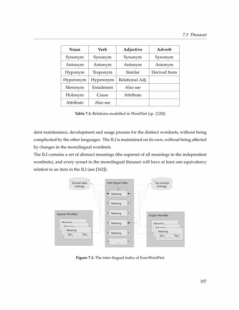
7.3 Thesauri
Noun Verb Adjective Adverb
Synonym Synonym Synonym Synonym
Antonym Antonym Antonym Antonym
Hyponym Troponym Similar Derived from
Hyperonym Hyperonym Relational Adj.
Meronym Entailment Also see
Holonym Cause Attribute
Attribute Also see
Table 7.1: Relations modelled in WordNet (cp. [120])
dent maintenance, development and usage process for the distinct wordnets, without being
complicated by the other languages. The ILI is maintained on its own, without being affected
by changes in the monolingual wordnets.
The ILI contains a set of abstract meanings (the superset of all meanings in the independent
wordnets), and every synset in the monolingual thesauri will have at least one equivalency
relation to an item in the ILI (see [162]).
Interlingual Index
English WordNet
Meaning
Syn1 ... Syn
nMeaning
Syn1 ... Syn
nMeaning
Syn1 ... Syn
n
Spanish WordNet
Meaning
Syn1 ... Syn
nMeaning
Syn1 ... Syn
nMeaning
Syn1 ... Syn
n
Meaning
Meaning
Meaning
Meaning
Meaning
...
Top conceptontology
Domain labelontology
Figure 7.1: The inter-lingual index of EuroWordNet
107
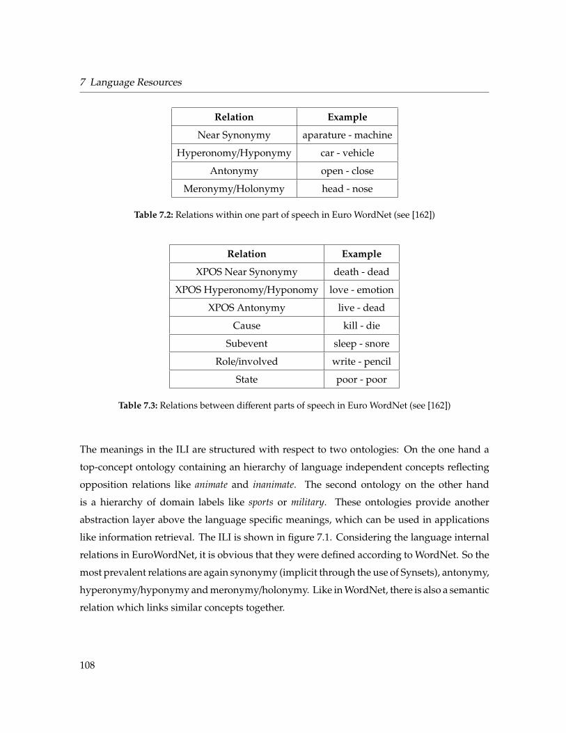
7 Language Resources
Relation Example
Near Synonymy aparature - machine
Hyperonomy/Hyponymy car - vehicle
Antonymy open - close
Meronymy/Holonymy head - nose
Table 7.2: Relations within one part of speech in Euro WordNet (see [162])
Relation Example
XPOS Near Synonymy death - dead
XPOS Hyperonomy/Hyponomy love - emotion
XPOS Antonymy live - dead
Cause kill - die
Subevent sleep - snore
Role/involved write - pencil
State poor - poor
Table 7.3: Relations between different parts of speech in Euro WordNet (see [162])
The meanings in the ILI are structured with respect to two ontologies: On the one hand a
top-concept ontology containing an hierarchy of language independent concepts reflecting
opposition relations like animate and inanimate. The second ontology on the other hand
is a hierarchy of domain labels like sports or military. These ontologies provide another
abstraction layer above the language specific meanings, which can be used in applications
like information retrieval. The ILI is shown in figure 7.1. Considering the language internal
relations in EuroWordNet, it is obvious that they were defined according to WordNet. So the
most prevalent relations are again synonymy (implicit through the use of Synsets), antonymy,
hyperonymy/hyponymy and meronymy/holonymy. Like in WordNet, there is also a semantic
relation which links similar concepts together.
108
7.3 Thesauri
In contrast to WordNet relations are labeled (e.g. a relation can be negated), and some relations
are allowed to exist between different syntactic categories. This makes it possible to define
similar meanings, antonymy or cause relations between for example verbs and nouns (e.g.
kill causes death). Furthermore the WordNet relation entailment is covered through the cause
relation and the additionally introduced subevent relation, which is more appealing to human
intuition. Another relation which was introduced is the role relation which specifies if e.g. a
verb describes a role a noun can occupy. An overview over the relations in EuroWordNet is
given in tables 7.2 and 7.3.
109

110
8 Building a System
The last chapters described existing architectures as well as processing and language re-
sources with their specific characteristics, requirements and implications. This chapter
will describe best practices to work with all those elements and to deal with mutual
dependencies. It will furthermore present strategies to select modules for a new sys-
tem.
8.1 Best Practices
Best practices are techniques and approaches which have proven to be more effective than
other methods given particular situations. Engineering language processing systems is no
exception, and therefore reveals strategies that are more successful, and approaches that are
error prone or less capable.
Without any claim to be complete, here are some best practices with respect to language
engineering:
1. Understanding the corpus. One of the biggest sins that can be committed in language
engineering is designing a system without even knowing the text. Methods as described
in chapter 4 help a lot in characterizing the text, but even then it is absolutely necessary
to read larger portions of the corpus, to get a general feeling about how the language
behaves. It should be sufficient to read several thousand words out of random samples,
and interesting aspects are found in abnormal morphology, syntax or terminology. Even
111
8 Building a System
if unsupervised methods are used, a text understanding is required to pick the right
modules, parameter settings and workflow definitions.
2. Independence of application. Processing resources should not be allowed to be aware
of the application they are used for. If information about the document is already
available beforehand (like language), it needs to be added to the document as a general
annotation, as would otherwise be done by the corresponding annotator. If additional
information needs to be conserved during the process (document id, user name etc.) it
can be added as an application specific annotation, which can be ignored by the analysis
modules. If for any reason a module is required to access or use application specific
data, the module is not usable in other contexts anymore. Although an architecture
should allow such modules, their usage should not be encouraged.
3. Centralization. There are three aspects to mention, which always need to be treated
uniformly and perhaps even centric in the framework itself: Tokenization, case and
encoding. Different usage of these concepts may lead to strange behavior and errors
that are hard to detect.
4. System evaluation. Regarding the complex (and scientifically neglected) interactions
and dependencies between modules, it is possible that a drastic accuracy increase of
one method does not change the system’s performance at all. As an example, spelling
accuracy might not hurt named entity extraction at all, if the spelling errors do not affect
the entity names (although they can still impurify the context, thereby complicating
machine learning methods). Especially systematic errors tend to have curious effects.
They can drastically decrease the performance of the whole system, or have no effects
at all, depending on which features are affected. Therefore a system always needs to be
evaluated as a whole, and errors need to be tracked back to the module that caused it.
5. Start with baselines. It is tempting to start developing a new system by implementing
and using best of breed methods. However, language processing methods are no
exception to the Pareto principle: 80% of the effect can normally be achieved with 20% of
112
8.1 Best Practices
the effort. Examples of this can be found frequently in language processing approaches.
A baseline part of speech tagger, which gives every known word its most frequent tag,
and unknown words a tag based on the last three letters, can already achieve an
accuracy of ca. 93% (see [30]). On the other hand a highly complex system as described
in [158] hardly exceeds 97%. A baseline named entity recognizer which only uses
lookup lists learned from training data can achieve precision values of up to 80% oder
90% with a recall between 40% and 70% (see [119]). Similar baseline methods exist
for tokenization (whitespace separation with separation of punctuation after words),
spelling correction (dictionary and edit distance) or language identification (using a
small set of function words as distinguishing features). A new system can be crafted
out of baseline algorithms significantly faster, and the baseline methods can still be
replaced with more effective approaches, if it turns out to be necessary after evaluating
the system as a whole (see above). Another argument in favor of baseline methods is
given by the fact that mutual dependencies sometimes require the usage of two similar
modules — e.g. a baseline named entity recognizer to improve spellchecking and part
of speech tagging, and a sophisticated entity recognizer which can then work on a better
foundation. Therefore a baseline method is usually not implemented in vain.
6. Usage of standardized knowledge bases. Language engineering systems use manifold
kinds of (enriched) lists with terminology. A language engineer may start with a
simple blacklist for stopword detection, later on add a dictionary of correct words for
spellchecking and a name list for named entity detection. While improving the system
it might be necessary to have separate kinds of stopwords (general ones, application
specific ones) and different classes of names (locations, person names, etc.) and at some
point every simple list gets more complicated. Flat hierarchies are added first and may
evolve to complex hierarchies, and sooner or later the entries get attributes (frequency,
part of speech, phonetic code, etc.) and relations between them — thereby ending up
with taxonomies, thesauri or ontologies. The worst case is reached, if every module
uses a resource in a different (proprietary) format using different access structures.
From a certain point of view it doesn’t even matter what kind of data structure is used
113
8 Building a System
— as long as it is standardized and used throughout the system. Even if it seems to be
an overhead in the beginning, very soon the additional effort pays of, and the advanced
capabilities will be utilized. The recommendation would be to select prior to system
construction one data structure able to do at least relations, attributes and hierarchies,
which is then used throughout the system.
7. Add simplified tagsets. Most off-the-shelf part of speech taggers use exhaustive tagsets,
containing dozens of different tags. The Penn Treebank Tagset (see [113]) for example
contains over 30 tags, the Stuttgart Tubingen Tagset (STTS1) even over 50 tags. Although
this level of detail is necessary for many applications, it is way too comprehensive
for others. Terminology extraction often filters for nouns, WordNet only covers the
major part of speech categories and if a user needs to work with the tagset (e.g. by
defining search queries or creating matching rules) he might be just overwhelmed by
such a huge set. Especially algorithms working on multilingual corpora might need
to find a common tagset across input languages, which is only possible by giving
up some level of detail. Therefore it can be recommended that no tagger should
be integrated into a system, without additionally annotating high level tags beside
the detailed ones. Although this can be achieved by adding an additional feature to
existing annotations, a better solution is to incorporate a second annotation type, or
using alternative annotations (see section 3.1.2).
8.2 Mutual Dependencies
Mutual dependencies can be found regularly in language processing systems, for example
between a tokenizer and language identification, or between part of speech tagging and
named entity recognition. These dependencies often lead to sloppy implementations which
are error prone and less accurate.
There are several different ways to resolve them:
1http://www.ims.uni-stuttgart.de/projekte/corplex/TagSets/stts-table.html
114
8.2 Mutual Dependencies
1. Avoidance. By revisiting the system’s requirements and goals, it might be possible to
rearrange modules or to choose a different approach for one of the modules, so that
the mutual dependency can be avoided. An example would be to switch from word
based language identification to character n-gram based identification if tokenization
needs to be language aware. Regarding robustness and runtime, this strategy is to be
preferred, but the avoidance of the problem is rarely possible.
2. Redundancy. By adding an additional baseline module with the same functionality
but reduced prerequisites, the problem can be solved by redundancy. This is often done
to resolve the dependency between named entity recognizer and part of speech taggers
or spellcheckers (see e.g. section 10.3.1). Both have problems with out-of-vocabulary
words, which are frequently names, but state of the art entity recognizers rely on correct
typing and part of speech tagging. By adding a baseline named entity recognizer (e.g.
list based) before spellchecking and tagging takes place, the actual entity annotator has
a better foundation to work on. This strategy is the pragmatic way to go. Accuracy
increases and the system architecture stays clearly arranged, with the drawback of
redundant modules. Given the fact that baseline methods are simple, fast to create and
often already available, this is a reasonable way to go.
3. Alternative Annotations. Ties can also be resolved by creating several alternative
annotations with different confidence values, which are later resolved by the other
module. This approach can for example be used to handle the mutual dependency
between spellchecking algorithms and syntactic methods. The spellchecker creates
several possible correction candidates and the part of speech tagger or syntax parser
sets the one which maximizes the probability of its own output.
4. Iteration. An iterative approach may be used, where all annotators create the most
accurate annotations they can, given the current information. With every iteration more
annotations, even from later stages of the workflow, are accessible and the accuracy of
the methods increases. This may especially pay of in bootstrapping scenarios, which
are iterative in nature. This approach is however highly instable and increases runtime
115

8 Building a System
drastically. Furthermore cascaded workflows are not directly supported in today’s
architectures (see chapter 3). Except in rare special cases, redundancy or avoidance
should be tried first.
8.3 A Proposal for System Building
Up to now this work left one question unanswered: How exactly is a language processing
system built? This section proposes a general approach to the problem, which is by all means
neither comprehensive nor in all cases applicable. For this scenario it is assumed that a
language engineer is confronted with a large corpus of unknown text and the goal of extracting
information. The following steps are suggested to bring the system on its way, by offering a
fast and reliable way to create a first set of baseline modules:
1. At first some randomly chosen parts of the corpus must be read. It makes sense to
manually review several hundred words in detail to get a feeling for part of speech
distributions, affix distributions, spelling quality and (lexical) ambiguities.
2. The next step is to determine the amount and fractions of different languages used in
the corpus. As language identification methods are portable enough (see section 6.1), a
pretrained baseline method can be employed to get a feeling for the different languages
in the corpus. As a tokenizer is not yet available, a character n-gram based method
is recommended, which is also more robust regarding misspellings, OCR errors and
other noise. As sentence boundaries are not yet detected, language identification must
be performed on document, paragraph, line or moving window level. Depending on
the results of this step, a more sophisticated language identification module can be
integrated and retrained if necessary.
3. The next module needed is a tokenizer, for which either a simple baseline approach or
a more sophisticated, but not yet adapted, mechanism is sufficient in the beginning.
It can be recommended to integrate a simple method based on regular expressions.
116
8.3 A Proposal for System Building
Even the first version must be able to identify and annotate numbers and punctuation
marks — although this can be done in separate modules, it is easier within a rule-based
tokenizer. The tokenization step needs to be language aware and fragments of the
corpus in different languages need to be processed separately.
4. Given the language identification and tokenization module, a first calculation of lan-
guage models should be performed. It is recommended to create models for character
n-grams, word n-grams (even monograms) and co-occurrences. All models need to
represent numbers and punctuation by unique placeholders, co-occurrences should
not yet be filtered for significances — the frequencies are a good basis to test several
significance measures and select an appropriate one.
5. Now a basic set of language characteristics can be derived (see chapter 4), and compared
to a familiar reference corpus. High values of concentration may indicate recurrent
elements like document headers, mail signatures or copyright remarks, or just doublets
in general. This can be verified by checking the top-n words. A high dispersion on the
other hand often indicates errors in tokenization, number detection or typing. Foreign
words can also lead to high dispersion or entropy values. These cases can be verified
by looking at low frequency words. The co-occurrences can be used to determine a
reasonable significance measure and to get a feeling for the semantics of the corpus,
and may even be used to identify frequent abbreviations (significant co-occurrence
with punctuation marks). These abbreviations can directly be used in a preliminary
abbreviation detection module, which facilitates sentence boundary detection. The
character n-grams calculated earlier are used to find and identify words which are
uncommon for the corpus and to get a first feeling for the morphological characteristics
of the corpus.
6. At this point the language identification module as well as the tokenizer (and num-
ber/punctuation detection) can be optimized and adapted using the knowledge gained
in the course of the last step.
117
8 Building a System
7. A data format for dictionaries, stopwords, domain terminology etc. must be chosen now
at the latest. It is recommended to use a standardized format consistently throughout
the workflow, which is at least capable of handling relations and attributes (see section
8.1). An efficient access structure is also important. Possible solutions are taxonomies,
thesauri, topic maps or lightweight ontologies.
8. A filtering module can be added to eliminate recurring elements and stopwords if
required. The blacklisted items are specified using the selected knowledge base.
9. An abbreviation detection module must be created to facilitate sentence boundary de-
tection. It can utilize the abbreviations which were identified above using co-occurrence
significances to punctuation marks. The abbreviations are also defined using the se-
lected knowledge base.
10. At this point a baseline sentence boundary detection is possible. If the tokenizer is able
to identify numbers reliably, and the abbreviation module detects the most common
abbreviations, a baseline sentence boundary detection can be created by just splitting
texts at the remaining punctuation marks.
11. A text cleaning step dealing with typographic errors can be added as needed, depending
on the spelling accuracy determined from reading a sample of text. Spelling correction
can be dictionary based if the vocabulary is restricted or typos are systematic. Unsuper-
vised approaches are chosen if feasible or if no time for dictionary creation is available.
However, keep in mind that spelling corrections are not yet performing well enough
to be used without careful evaluation — they are likely to introduce more errors than
they resolve, depending on the amount of out-of-vocabulary words, real-word errors
and dictionary size (see section 6.3).
12. Finally, the workflow created so far can be used to recreate language models and
recalculate language characteristics.
118
8.3 A Proposal for System Building
After these steps, a basic set of baseline modules for text preprocessing is available. Quality
is already supposed to be sufficient for many applications, but needs to be verified, evaluated
and optimized. Every additional module is increasingly harder to choose, design/adapt and
implement:
1. It is recommended to always include a part of speech tagging module, as its usages
are manifold for filtering, abstraction, machine learning etc. If the corpus requires
retraining of a part of speech tagger because of special terminology, unusual syntax
or morphology, an unsupervised tagger can be considered, as manual annotation of a
training set may hit time constraints. Otherwise an off-the-shelf tagger can be evaluated,
and retrained on an automatically tagged and manually reviewed training set. A good
choice is probably the Brill tagger (see [30]), as its rules are easy to adapt and change
manually.
2. Given the part of speech tagger obtained in the last step, a basic set of domain terminol-
ogy can be extracted. As most algorithms do not perform well enough for automatic
usage (see section 10.5.1), the results need to be reviewed. Multi-word as well as
single-word terminology should be extracted and a synonym extraction step should
also be performed. As manual correction is unavoidable anyways, baseline algorithms
are sufficient here. Although synonym extraction algorithms are known to extract
co-hyponyms, hyperonyms or antonyms (see [166, chapter 3.3 ff]) beside synonyms,
those terms are also useful and can be added to the knowledge bases. If remaining
misspellings are detected as synonyms, the spelling correction step might need to be
adjusted or extended.
3. If the entities to extract are given by a closed group of rarely ambiguous items, a
knowledge based approach is a good start. If the entities belong to an open class or are
highly ambiguous, the context needs to be considered using pattern based approaches
or machine learning. Either way, a taxonomy, thesaurus or word-net as created in the
last step is very helpful. Even if there is no predefined one available for the given
119
8 Building a System
corpus or task, it always makes sense to start a new one which can be populated while
going on.
4. The final relation extraction step depends on the task to perform. A good advice is
to manually review several examples of relations and their contexts. The degree to
which the contexts imply an instance of the relation can be seen as an indicator of
the difficulties to expect. Often an additional parser is needed, but its usage must be
carefully reviewed, and maybe even neglected in favor of shallow (e.g. as in [173]) or
chunk parsing. In general pattern based methods in combination with bootstrapping
are a good start. If they perform well the problem is solved, if not they still give a good
baseline to evaluate more sophisticated methods and to increase the training data.
After having created all those modules, it is important to test and evaluate the system as a
whole. Errors can be tracked back to the erroneous components and the baseline modules
can be improved iteratively as needed.
120
Part II
Language Engineering for
Automotive Quality Analysis
121

9 Quality Analysis on Automotive Domain
Language
This chapter describes the usecase from the automotive domain which is used to illustrate
the findings of part I. After introducing the domain with its application requirements the
textual data will be characterized and a first sketch of the language engineering system is
outlined.
9.1 Automotive Quality Analysis
Quality assurance can be seen as a crucial process for every company. A fast detection of
product deficits is required for taking countermeasures, to ensure customer satisfaction and
to uphold brand perception. Quality problems may also raise legal issues or even impact
the customer’s safety. The usecase for this work is given by the quality analysis research
of an international manufacturer of premium vehicles — the Daimler AG. Although the
company has sophisticated and comprehensive processes for the analysis of quality data, the
tools and methods to work with unstructured data are still limited. This work tries to close
this gap, by providing efficient and high accuracy means to preprocess and analyze textual
data.
123
9 Quality Analysis on Automotive Domain Language
9.1.1 Structured Quality Data
Data for quality analysis is consequently and broadly gathered from dealerships, press and
media, customer studies and field tests, thereby leaving huge amounts of data to be handled
and understood. The predominant source of quality field data is given by everyday repair
orders from dealerships. Given the international dissemination of Daimler brand vehicles,
it is clear that every single day of data may contain up to several hundred thousand repair
order cases. Quality analysis is historically focused on the structured data provided for these
repairs, given by one or more of the following items:
1. Damage codes denoting the kind of problem detected and all of the affected compo-
nents. There may be several codes per repair order denoting subproblems or follow up
damages.
2. Date of repair.
3. Vehicle Identification Number (VIN) of the car.
4. ZIP code and country of the dealership.
5. Model year and model family of the car.
6. Mileage of the car.
7. Production date of the car.
8. Built in extras of the car. Besides series equipment like air conditioning or eight way
seats, this can also be special equipment as used for example in police cars.
Although this data seems to be very comprehensive, it still suffers from at least two severe
drawbacks:
124
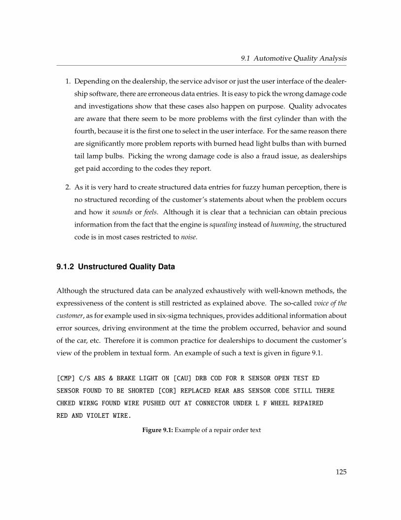
9.1 Automotive Quality Analysis
1. Depending on the dealership, the service advisor or just the user interface of the dealer-
ship software, there are erroneous data entries. It is easy to pick the wrong damage code
and investigations show that these cases also happen on purpose. Quality advocates
are aware that there seem to be more problems with the first cylinder than with the
fourth, because it is the first one to select in the user interface. For the same reason there
are significantly more problem reports with burned head light bulbs than with burned
tail lamp bulbs. Picking the wrong damage code is also a fraud issue, as dealerships
get paid according to the codes they report.
2. As it is very hard to create structured data entries for fuzzy human perception, there is
no structured recording of the customer’s statements about when the problem occurs
and how it sounds or feels. Although it is clear that a technician can obtain precious
information from the fact that the engine is squealing instead of humming, the structured
code is in most cases restricted to noise.
9.1.2 Unstructured Quality Data
Although the structured data can be analyzed exhaustively with well-known methods, the
expressiveness of the content is still restricted as explained above. The so-called voice of the
customer, as for example used in six-sigma techniques, provides additional information about
error sources, driving environment at the time the problem occurred, behavior and sound
of the car, etc. Therefore it is common practice for dealerships to document the customer’s
view of the problem in textual form. An example of such a text is given in figure 9.1.
[CMP] C/S ABS & BRAKE LIGHT ON [CAU] DRB COD FOR R SENSOR OPEN TEST ED
SENSOR FOUND TO BE SHORTED [COR] REPLACED REAR ABS SENSOR CODE STILL THERE
CHKED WIRNG FOUND WIRE PUSHED OUT AT CONNECTOR UNDER L F WHEEL REPAIRED
RED AND VIOLET WIRE.
Figure 9.1: Example of a repair order text
125
9 Quality Analysis on Automotive Domain Language
Advantages of such a text are especially that nobody states a wrong damage by mistake or
out of laziness. Textual descriptions might be written sloppy or fuzzy, but they are normally
correct, unless the writer acts intentionally (e.g. in fraud cases). Furthermore they provide
a higher level of detail than the structured data does, especially with respect to error con-
ditions ("happens only when cold") and descriptions ("a high pinching noise when driving
over bumps"). But it is obvious that every analysis of those texts is complicated and error
prone, given by their nature. They are gathered in several languages, written sloppy and full
of technical terms, ambiguous abbreviations and technical codes.
The following chapters will document how such highly domain specific language
can be handled, and how a system for the analysis can be planned and imple-
mented.
9.1.3 Quality Analysis Tasks
Of all quality analysis tasks, which are performed by an automotive company, this work pro-
vides means for incorporating textual data in three major processes. Early warning methods
try to detect a problem as soon as possible, to minimize negative experiences by customers,
provide quick solutions and avoid safety issues. Besides the principal effort to offer customers
the best possible support, this is very important for brand perception — fixing problems be-
fore the media attention is getting high is crucial. Section 11.2 investigates the usage of textual
data for early warning.
Root Cause Analysis tries to find the reasons for a rising number of repairs. There are often
cases where a part fails, but it is unclear why. Reasons can be found in complicated technical
interactions, but also in environment conditions (cold weather, sandy roads, cars delivered
by ship, etc.) and driving conditions (only driven in cities, rarely driven, etc.). Root cause
analysis offers great possibilities for the usage of textual data, as the customer often enough
knows and even states these conditions. A scenario using texts for root cause analysis is
described in section 11.1.
Repeat Repair Detection tries to calculate the so-called Fixed-First-Visit (FFV) rate. This rate
126
9.2 Domain Requirements
states how often a customer needs to come back to a dealership to get a problem fixed.
It is obvious that a low FFV rate indicates a bad dealership performance and leads to
a negative brand perception. A good example for the benefits of textual data for re-
peat repair detection is described in [82] and omitted here due to the straightforward ap-
proach.
9.2 Domain Requirements
No language processing system can be designed to achieve all possible tasks, and some-
times they are carefully tailored to the demands of a special application. Therefore the
requirements from the application side of the automotive usecase need to be consid-
ered:
1. Components, failure symptoms and corrective measures must be detected as well as the
relations between each other. Although this seems to be a classical case for information
extraction methods, it needs to be noted that the entities comprise unnamed concepts
(like common verbs or adjectives) and that relations are expressed via syntactic means
like head-modifier relations.
2. Analysis must be deterministic — if a quality advocate is doing the same evaluation
twice, the results must be identical.
3. Analysis must work even for a single text with predictable results. Quality studies are
sometimes performed on small subsets as for example the analysis of a specific model
of a specific model-year in a specific calendar month — of which perhaps only several
ten cases are available. This hinders the usage of statistical methods, which rely on
large data sets.
4. Handling of English language text has priority. However the system should be designed
to allow the extension to other languages.
127
9 Quality Analysis on Automotive Domain Language
5. The system needs to target high precision in favor of high recall. Although it is hard
to accept that information may be lost, high quality of results must be ensured. A
company cannot afford to start countermeasures like recalls or service campaigns based
on doubtful data. A low recall is furthermore compensated by the high amount of
redundant repair cases.
6. Textual data is thought of as addition to the analysis of structured data. It should not
and is not allowed to replace the traditional quality analysis on structured data.
9.3 Textual Data
The data used in this part is gathered from automotive dealerships belonging to Daimler.
Although the texts are systematically recorded only in the US, they contain up to 4% of
Spanish and French documents which are gathered from Spanish and French speaking areas
in Canada, Mexico or along the US border.
The texts are normally very short (e.g. several ten words) and even a quick glance over the
data shows a high fraction of technical codes, numbers, abbreviations and spelling errors.
The biggest part of the texts are capitalized, and whitespace other than blanks is removed
during the gathering process.
To get a feeling for these documents, the characteristics of the corpus are calculated
as described in chapter 4 and the results are depicted in figure 9.2. The figure
also shows news texts for comparison, as those are used broadly in other scientific
works.
The figure clearly shows that the domain language differs massively from news language. On
the one hand they have shorter sentences containing less grammatical constructs. But on the
other hand they are much more predictable and have a significantly smaller vocabulary size.
The high dispersion of the corpus derives on the one hand from the low spelling accuracy, and
on the other hand is influenced by tokenization errors. Remember that those characteristics
128
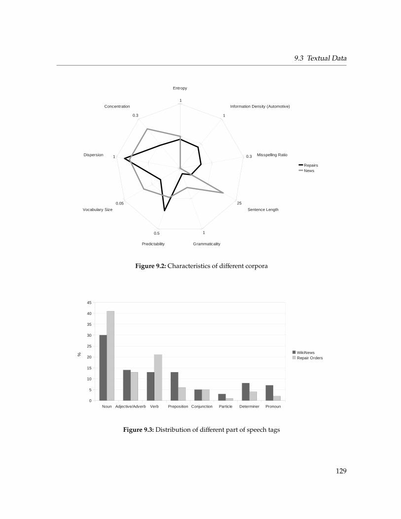
9.3 Textual Data
Entropy
Concentration
Dispersion
Vocabulary Size
Predictability Grammaticality
Sentence Length
Misspelling Ratio
Information Density (Automotive)
RepairsNews
1
1
1
0.3
25
1
0.3
0.05
0.5
Figure 9.2: Characteristics of different corpora
Noun Adjective/Adverb Verb Preposition Conjunction Particle Determiner Pronoun
0
5
10
15
20
25
30
35
40
45
WikiNewsRepair Orders
%
Figure 9.3: Distribution of different part of speech tags
129
9 Quality Analysis on Automotive Domain Language
are calculated on purpose without methods adapted to this domain, as they should show us
which methods to chose and how to apply and tune them.
Figure 9.3 shows the distribution of part of speech tags in the two corpora. Here again
the strong difference of the two domains is visible by a significantly different distribution.
The domain dependent repair order texts show a high amount of nouns and verbs to the
cost of nearly all other word classes. This illustrates the high information density of the
texts.
9.4 Outlining the System
Considering the requirements given in section 9.2 and the characteristics of the textual data
described in section 9.3 a first sketch of the resulting system can be done.
As the amount of non-English texts is significantly higher than the error rate of current
language identification algorithms (see section 6.1), the inclusion of a language identifier is
useful, and may provide a solid base for later extensions to the system.
The high dispersion of the language combined with the high fraction of codes and numbers
requires the usage of a sophisticated tokenization mechanism. Considering the current tech-
nologies for tokenization (see section 6.2) it becomes clear that a rule based method should be
employed with a set of handcrafted rules. As those rules can be optimized iteratively during
system build-up and will also be reusable for other languages after manual adjustments, the
benefits are worth the effort.
After those two steps are finished, the calculation of co-occurrences, word and letter n-grams
should be performed. The high value for predictability and the low vocabulary size show that
those models can be calculated easily, and will not grow as large as for other languages.
Together with a careful pruning step (justified by the high dispersion and the low spelling
accuracy) these models can be employed very effectively.
To deal with the high amount of misspellings (dependent on the specific writer up to 20%)
a spellchecking step seems to be sensible. Although automatic spelling correction is still
not reaching high accuracy (see section 6.3) it can be employed to this domain due to the
130
9.5 The Architecture
small vocabulary size and high predictability. Regarding the characteristics of the corpus a
spellchecking method based on word bigrams or neighborhood co-occurrences will be a
good choice.
Given a small lexical ambiguity together with small grammaticality and short average sentence
length, the usage of rather basic part of speech tagging and syntactic parsing solutions seems
appropriate, and even the usage of unsupervised approaches may provide sound results.
Entity detection is best performed by dictionary based approaches, as especially the most
important class of car components can be exhaustively enumerated, and is even available
via existing sources. Smaller ambiguities may be resolved through context keywords or part
of speech tags.
The relation extraction step is harder to decide and may need further experi-
ments.
9.5 The Architecture
The implementation of the system is based on the UIMA architecture (see [54]). Based
on the findings in chapter 3 UIMA was chosen because of its programmatic access, the
standardization efforts, the healthy community and infrastructural features like language-
aware parameter sets and type system inheritance.
All modules described in the following sections are designed as UIMA annotators enriching
the text with stand-off annotations using the JCas model defined by the architecture. Data
is read in from varying formats using UIMA Collection-Readers, and outputs are saved in
various ways like CSV, XML or relational databases.
131

132
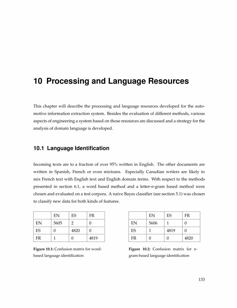
10 Processing and Language Resources
This chapter will describe the processing and language resources developed for the auto-
motive information extraction system. Besides the evaluation of different methods, various
aspects of engineering a system based on those resources are discussed and a strategy for the
analysis of domain language is developed.
10.1 Language Identification
Incoming texts are to a fraction of over 95% written in English. The other documents are
written in Spanish, French or even mixtures. Especially Canadian writers are likely to
mix French text with English text and English domain terms. With respect to the methods
presented in section 6.1, a word based method and a letter-n-gram based method were
chosen and evaluated on a test corpora. A naive Bayes classifier (see section 5.1) was chosen
to classify new data for both kinds of features.
EN ES FR
EN 5605 2 0
ES 0 4820 0
FR 1 0 4819
Figure 10.1: Confusion matrix for word-
based language identification
EN ES FR
EN 5606 1 0
ES 1 4819 0
FR 0 0 4820
Figure 10.2: Confusion matrix for n-
gram-based language identification
133
10 Processing and Language Resources
The set was constructed by automatic means, manually corrected and contains around 60.000
documents from the domain, with approx. 20.000 documents of each language. Three quar-
ters of the texts were chosen as training data for the two methods, the rest is used for testing.
The results can be seen in tables 10.1 and 10.2. In general both algorithms perform very good,
although the n-gram based method reached the given performance only for quadgrams and
higher order n-grams. A set of additional experiments with the same classifiers trained on
other corpora of the given languages revealed however a higher portability of the n-gram
based method. While both methods achieved an accuracy of approx. 98% for English and
Spanish after training on other corpora, the word based method had problems with French
text. This was due to a high fraction of French domain texts without proper usage of diacritics
and should therefore not be overrated. As the letter n-gram solution is however easier to
adapt to other languages and does not introduce mutual dependencies with the tokenization
step, it is the preferred choice for the system.
As language identification for mixed documents does not yet reach the required perfor-
mance, and mixed language documents are not supported by current language engineering
architectures, all documents are annotated on a per document level. Every succeeding step
of the architecture is performed language aware, but with a strong focus on English docu-
ments.
10.2 Tokenization
As the texts contain a high fraction of domain specific codes and number formats (indicated
by a high dispersion), a flexible approach to tokenization is needed. With respect to the results
derived in section 6.2 a rule based method was chosen and implemented using prioritized
regular expressions. The approach is based on the one described in further detail in [104,
chapter 5.3.2].
Beside the straight-forward approach on the method side, more sophisticated models are
implemented on the type-system side. The tokenizer heavily relies on type-system inheri-
tance by defining an annotation Token, which serves as a superclass for more specialized token
134
10.3 Spelling Correction
types for numbers, codes, real-words, URLs and even smilies. The classes are generated from
the abstract type system definition, and subclasses are manually adapted to reflect distinct
behavior. All tokens declare for example methods to return a normalized representation and
a method to return a replacement string for the calculation of n-grams and co-occurrences. A
token (e.g. 20000km) representing a number can therefore override both methods and return
a localized and normalized version of itself in the first method (e.g. 12.427miles), and return
a placeholder like $NUMBER$ in the second. This ensures not only consistent behavior
throughout the system, but also simplifies language model calculation and fosters code reuse
and maintainability. More sophisticated models may even implement different behaviors
depending on the reading direction. A sentence boundary can return different placeholders
for the left and the right side, thereby reflecting its different functions as sentence start and
sentence end.
10.3 Spelling Correction
As seen in section 9.3 the documents have a low spelling accuracy of approx. 90% on average
and up to 20% or more of misspellings depending on the author and dealership. Besides
the pure typographical errors there is also a large fraction of abbreviations, which are partly
ambiguous. The amount of realword errors is small, enabling the use of dictionary based
approaches as outlined in section 6.3. Another indicator for the usage of knowledge-based
spelling correction techniques is the small vocabulary size (see section 9.3) of the corpus.
Context clues can also be used for correction due to the high predictability of the corpus, and
can be employed through word n-gram models or co-occurrences.
As a high precision needs to be achieved by the system (see section 9.2), the correction
strategy needs to be conservative, meaning that a word is only corrected if several tight
thresholds are met.
With respect to the requirements and preconditions, a dictionary-based approach similar
135
10 Processing and Language Resources
to the well-known ASpell1 algorithm is chosen and extended by frequency lists and con-
text clues given by neighborhood co-occurrences. Abbreviations are replaced in a context
sensitive way based on replacement lists. These lists are furthermore used to speed-up the
handling of very common spelling errors.
The spellchecking process is divided into several modules on the architectural side. Hierar-
chical workflows or the definition of processing resources made up of other modules needs
to be supported by the language engineering infrastructure and is in this case provided
by UIMA. Language resources like dictionaries, rules for the creation of phonetic codes
and general thresholds are loaded language aware, and all resources are loaded only once.
Every correction made by the system replaces the original token annotation with a special
SpellingCorrection annotation, which is a subtype of token. A better solution would be the
usage of alternative annotations, which are unfortunately not provided by current language
engineering architectures. If both annotations would be kept, every following module would
need to be aware of this, thereby massively hindering reusability and exchangeability of
modules.
A first variant of the approach described here was presented in [104].
10.3.1 Baseline Named Entity Detection
To avoid the detection of named entities as misspellings, they are identified using a high recall
baseline method in a first step. After detecting common first names as given by simple lists,
the following token is checked. If it can not be found in the dictionary of correct words, it is
marked as surname. This approach has several advantages. Besides being fast and simple
to implement, it offers high recall. The probability to spellcheck and falsely correct a name
is therefore practically eliminated. If a surname is missed because it is also in the dictionary,
it would not have been corrected anyways and therefore no additional source of errors is
introduced. The low precision of the approach might lead to real typographic errors which
1http://aspell.net/
136
10.3 Spelling Correction
go now undetected — but this happens rarely and is fine regarding the overall goal to not
introduce new errors with the spellchecking.
10.3.2 Replacements
The next module handles all kinds of replacements, to deal with general and custom abbrevi-
ations which cannot easily be handled by a pure spelling correction algorithm. Replacement
lists R were manually created to replace those abbreviations as well as certain multi-word-
terms and very frequent and hard to correct misspellings. The replacement module works
on tokens as defined in the type hierarchy, uses language dependent resources and incorpo-
rates context information. This is needed for the replacement of ambiguous abbreviations
as the following example illustrates. If the module finds the word lt, it can mean both
light and left. To handle this, the algorithm looks up the co-occurrence levels of each pos-
sible replacement w as left neighbor of the succeeding word Cooc(w,wright) and as right
neighbor of the preceding word Cooc(wle f t,w). The result is the replacement w′ with the
maximum co-occurrence level to the left neighbor word wle f t or to the right neighbor word
wright.
Cooc(w) = max(Cooc(wle f t,w) , Cooc(w,wright)) (10.1)
w′ = argmaxw∈R
(Cooc(w)) (10.2)
10.3.3 Merging
To merge words which where split by an unintended blank character, this module sequen-
tially checks two adjacent words for correct spelling. If one or both words are not contained in
the dictionary (and have a minimum word length), but the joint word is, a spelling correction
candidate annotation is generated, which contains a merged representation. The candidate is
verified with respect to the left and right neighbors. If it fits to the context, the candidate is ac-
cepted immediately, as the probability to generate erroneous corrections by concatenating real
words is pretty small (at least for the given English corpus).
137
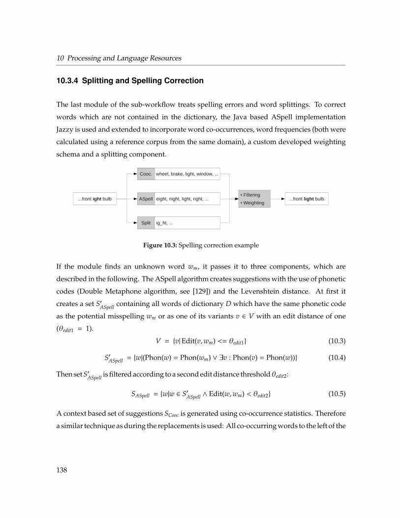
10 Processing and Language Resources
10.3.4 Splitting and Spelling Correction
The last module of the sub-workflow treats spelling errors and word splittings. To correct
words which are not contained in the dictionary, the Java based ASpell implementation
Jazzy is used and extended to incorporate word co-occurrences, word frequencies (both were
calculated using a reference corpus from the same domain), a custom developed weighting
schema and a splitting component.
...front ight bulb
wheel, brake, light, window, ...Cooc.
eight, night, light, right, ...ASpell● Filtering
● Weighting
ig_ht, ...Split
...front light bulb
Figure 10.3: Spelling correction example
If the module finds an unknown word wm, it passes it to three components, which are
described in the following. The ASpell algorithm creates suggestions with the use of phonetic
codes (Double Metaphone algorithm, see [129]) and the Levenshtein distance. At first it
creates a set S′ASpell containing all words of dictionary D which have the same phonetic code
as the potential misspelling wm or as one of its variants v ∈ V with an edit distance of one
(θedit1 = 1).
V = {v|Edit(v,wm) <= θedit1} (10.3)
S′ASpell = {w|(Phon(w) = Phon(wm) ∨ ∃v : Phon(v) = Phon(w))} (10.4)
Then set S′ASpell is filtered according to a second edit distance thresholdθedit2:
SASpell = {w|w ∈ S′ASpell ∧ Edit(w,wm) < θedit2} (10.5)
A context based set of suggestions SCooc is generated using co-occurrence statistics. Therefore
a similar technique as during the replacements is used: All co-occurring words to the left of the
138
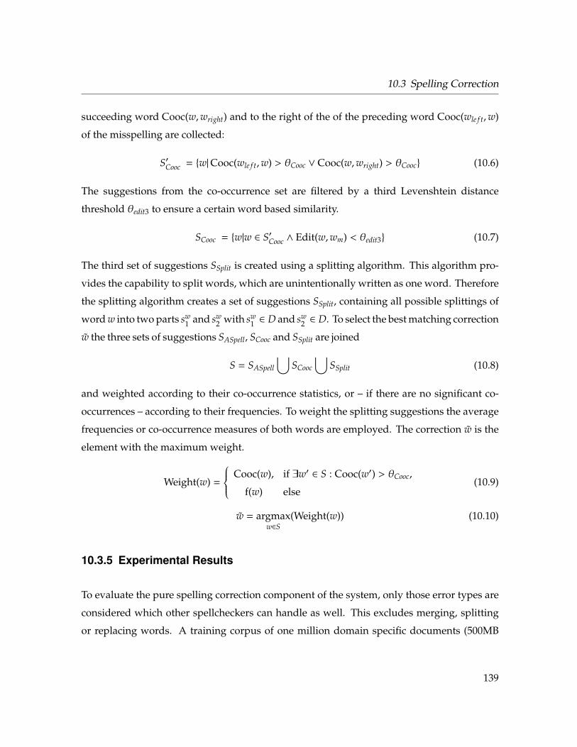
10.3 Spelling Correction
succeeding word Cooc(w,wright) and to the right of the of the preceding word Cooc(wle f t,w)
of the misspelling are collected:
S′Cooc = {w|Cooc(wle f t,w) > θCooc ∨ Cooc(w,wright) > θCooc} (10.6)
The suggestions from the co-occurrence set are filtered by a third Levenshtein distance
threshold θedit3 to ensure a certain word based similarity.
SCooc = {w|w ∈ S′Cooc ∧ Edit(w,wm) < θedit3} (10.7)
The third set of suggestions SSplit is created using a splitting algorithm. This algorithm pro-
vides the capability to split words, which are unintentionally written as one word. Therefore
the splitting algorithm creates a set of suggestions SSplit, containing all possible splittings of
word w into two parts sw1 and sw
2 with sw1 ∈ D and sw
2 ∈ D. To select the best matching correction
w the three sets of suggestions SASpell, SCooc and SSplit are joined
S = SASpell
⋃SCooc
⋃SSplit (10.8)
and weighted according to their co-occurrence statistics, or – if there are no significant co-
occurrences – according to their frequencies. To weight the splitting suggestions the average
frequencies or co-occurrence measures of both words are employed. The correction w is the
element with the maximum weight.
Weight(w) =
Cooc(w), if ∃w′ ∈ S : Cooc(w′) > θCooc,
f(w) else(10.9)
w = argmaxw∈S
(Weight(w)) (10.10)
10.3.5 Experimental Results
To evaluate the pure spelling correction component of the system, only those error types are
considered which other spellcheckers can handle as well. This excludes merging, splitting
or replacing words. A training corpus of one million domain specific documents (500MB
139
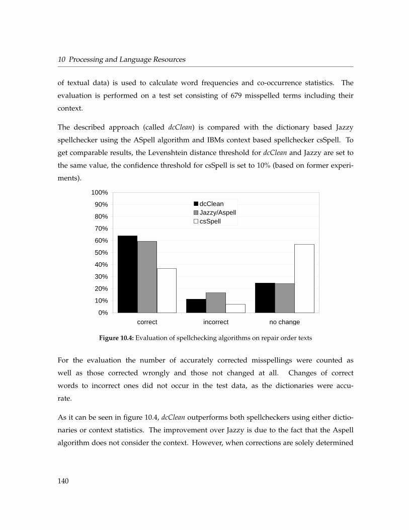
10 Processing and Language Resources
of textual data) is used to calculate word frequencies and co-occurrence statistics. The
evaluation is performed on a test set consisting of 679 misspelled terms including their
context.
The described approach (called dcClean) is compared with the dictionary based Jazzy
spellchecker using the ASpell algorithm and IBMs context based spellchecker csSpell. To
get comparable results, the Levenshtein distance threshold for dcClean and Jazzy are set to
the same value, the confidence threshold for csSpell is set to 10% (based on former experi-
ments).
0%
10%
20%
30%
40%
50%
60%
70%
80%
90%
100%
correct incorrect no change
dcCleanJazzy/AspellcsSpell
Figure 10.4: Evaluation of spellchecking algorithms on repair order texts
For the evaluation the number of accurately corrected misspellings were counted as
well as those corrected wrongly and those not changed at all. Changes of correct
words to incorrect ones did not occur in the test data, as the dictionaries were accu-
rate.
As it can be seen in figure 10.4, dcClean outperforms both spellcheckers using either dictio-
naries or context statistics. The improvement over Jazzy is due to the fact that the Aspell
algorithm does not consider the context. However, when corrections are solely determined
140
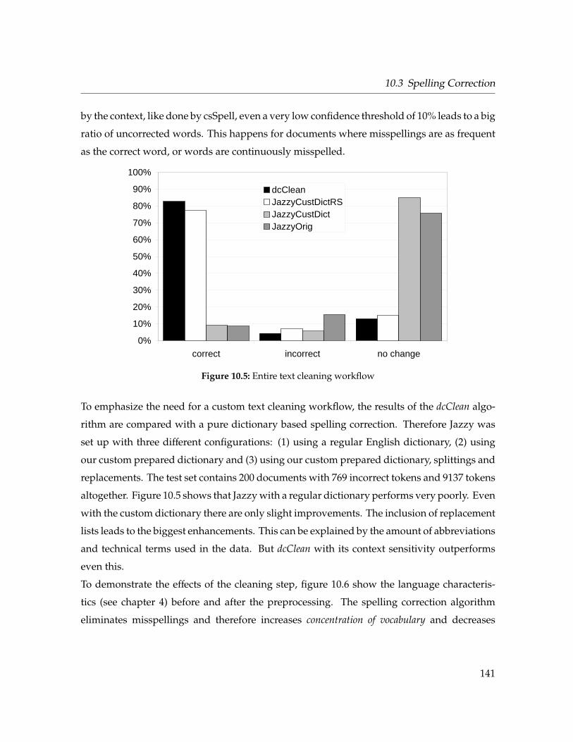
10.3 Spelling Correction
by the context, like done by csSpell, even a very low confidence threshold of 10% leads to a big
ratio of uncorrected words. This happens for documents where misspellings are as frequent
as the correct word, or words are continuously misspelled.
0%
10%
20%
30%
40%
50%
60%
70%
80%
90%
100%
correct incorrect no change
dcCleanJazzyCustDictRSJazzyCustDictJazzyOrig
Figure 10.5: Entire text cleaning workflow
To emphasize the need for a custom text cleaning workflow, the results of the dcClean algo-
rithm are compared with a pure dictionary based spelling correction. Therefore Jazzy was
set up with three different configurations: (1) using a regular English dictionary, (2) using
our custom prepared dictionary and (3) using our custom prepared dictionary, splittings and
replacements. The test set contains 200 documents with 769 incorrect tokens and 9137 tokens
altogether. Figure 10.5 shows that Jazzy with a regular dictionary performs very poorly. Even
with the custom dictionary there are only slight improvements. The inclusion of replacement
lists leads to the biggest enhancements. This can be explained by the amount of abbreviations
and technical terms used in the data. But dcClean with its context sensitivity outperforms
even this.
To demonstrate the effects of the cleaning step, figure 10.6 show the language characteris-
tics (see chapter 4) before and after the preprocessing. The spelling correction algorithm
eliminates misspellings and therefore increases concentration of vocabulary and decreases
141
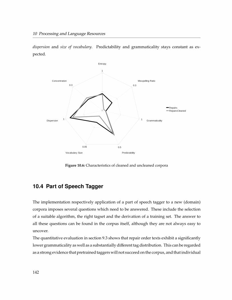
10 Processing and Language Resources
dispersion and size of vocabulary. Predictability and grammaticality stays constant as ex-
pected.
Entropy
Concentration
Dispersion
Vocabulary Size Predictability
Grammaticality
Misspelling Ratio
RepairsRepairsCleaned
1
1 1
0.30.3
0.05 0.5
Figure 10.6: Characteristics of cleaned and uncleaned corpora
10.4 Part of Speech Tagger
The implementation respectively application of a part of speech tagger to a new (domain)
corpora imposes several questions which need to be answered. These include the selection
of a suitable algorithm, the right tagset and the derivation of a training set. The answer to
all these questions can be found in the corpus itself, although they are not always easy to
uncover.
The quantitative evaluation in section 9.3 shows that repair order texts exhibit a significantly
lower grammaticality as well as a substantially different tag distribution. This can be regarded
as a strong evidence that pretrained taggers will not succeed on the corpus, and that individual
142
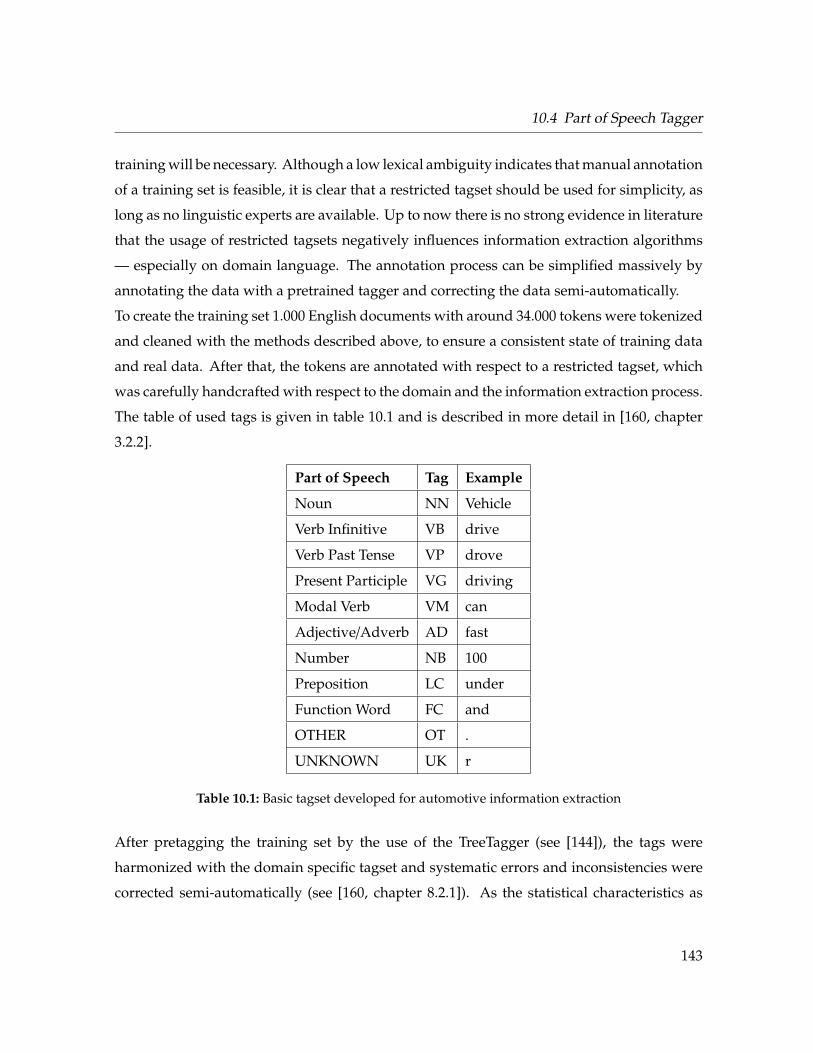
10.4 Part of Speech Tagger
training will be necessary. Although a low lexical ambiguity indicates that manual annotation
of a training set is feasible, it is clear that a restricted tagset should be used for simplicity, as
long as no linguistic experts are available. Up to now there is no strong evidence in literature
that the usage of restricted tagsets negatively influences information extraction algorithms
— especially on domain language. The annotation process can be simplified massively by
annotating the data with a pretrained tagger and correcting the data semi-automatically.
To create the training set 1.000 English documents with around 34.000 tokens were tokenized
and cleaned with the methods described above, to ensure a consistent state of training data
and real data. After that, the tokens are annotated with respect to a restricted tagset, which
was carefully handcrafted with respect to the domain and the information extraction process.
The table of used tags is given in table 10.1 and is described in more detail in [160, chapter
3.2.2].
Part of Speech Tag Example
Noun NN Vehicle
Verb Infinitive VB drive
Verb Past Tense VP drove
Present Participle VG driving
Modal Verb VM can
Adjective/Adverb AD fast
Number NB 100
Preposition LC under
Function Word FC and
OTHER OT .
UNKNOWN UK r
Table 10.1: Basic tagset developed for automotive information extraction
After pretagging the training set by the use of the TreeTagger (see [144]), the tags were
harmonized with the domain specific tagset and systematic errors and inconsistencies were
corrected semi-automatically (see [160, chapter 8.2.1]). As the statistical characteristics as
143
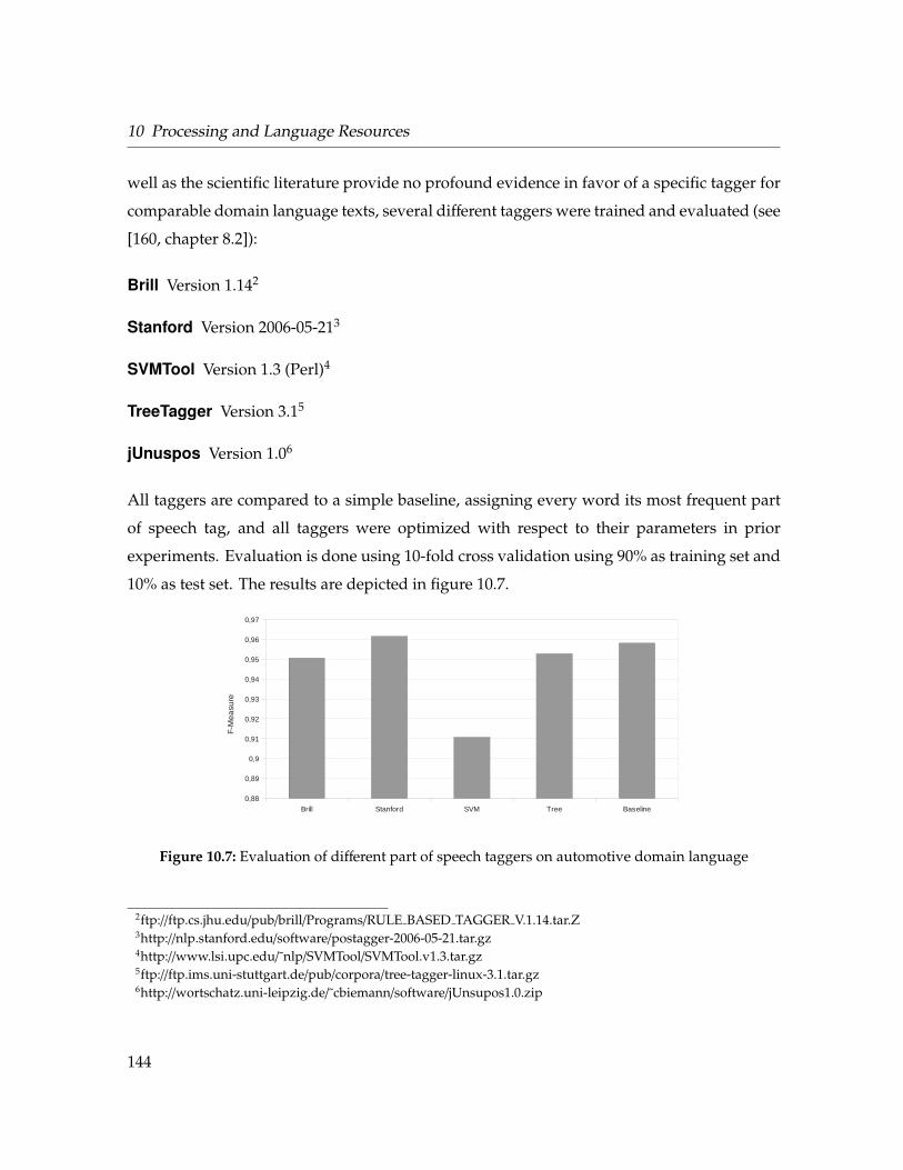
10 Processing and Language Resources
well as the scientific literature provide no profound evidence in favor of a specific tagger for
comparable domain language texts, several different taggers were trained and evaluated (see
[160, chapter 8.2]):
Brill Version 1.142
Stanford Version 2006-05-213
SVMTool Version 1.3 (Perl)4
TreeTagger Version 3.15
jUnuspos Version 1.06
All taggers are compared to a simple baseline, assigning every word its most frequent part
of speech tag, and all taggers were optimized with respect to their parameters in prior
experiments. Evaluation is done using 10-fold cross validation using 90% as training set and
10% as test set. The results are depicted in figure 10.7.
Brill Stanford SVM Tree Baseline
0,88
0,89
0,9
0,91
0,92
0,93
0,94
0,95
0,96
0,97
F-M
easu
re
Figure 10.7: Evaluation of different part of speech taggers on automotive domain language
2ftp://ftp.cs.jhu.edu/pub/brill/Programs/RULE BASED TAGGER V.1.14.tar.Z3http://nlp.stanford.edu/software/postagger-2006-05-21.tar.gz4http://www.lsi.upc.edu/˜nlp/SVMTool/SVMTool.v1.3.tar.gz5ftp://ftp.ims.uni-stuttgart.de/pub/corpora/tree-tagger-linux-3.1.tar.gz6http://wortschatz.uni-leipzig.de/˜cbiemann/software/jUnsupos1.0.zip
144
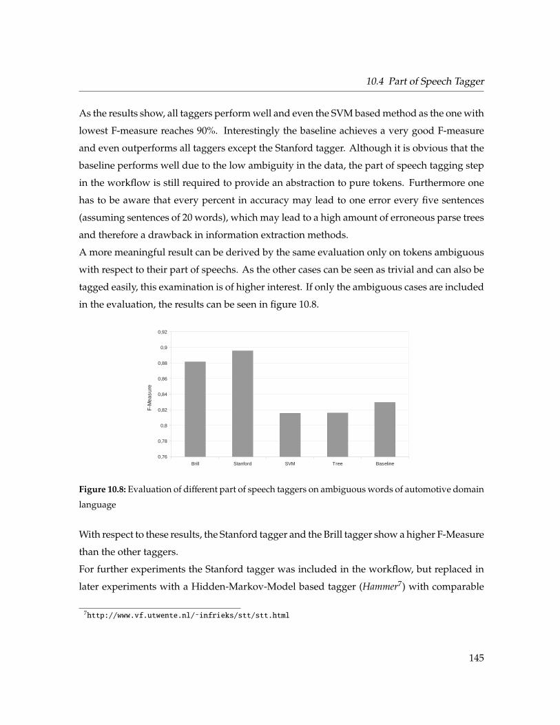
10.4 Part of Speech Tagger
As the results show, all taggers perform well and even the SVM based method as the one with
lowest F-measure reaches 90%. Interestingly the baseline achieves a very good F-measure
and even outperforms all taggers except the Stanford tagger. Although it is obvious that the
baseline performs well due to the low ambiguity in the data, the part of speech tagging step
in the workflow is still required to provide an abstraction to pure tokens. Furthermore one
has to be aware that every percent in accuracy may lead to one error every five sentences
(assuming sentences of 20 words), which may lead to a high amount of erroneous parse trees
and therefore a drawback in information extraction methods.
A more meaningful result can be derived by the same evaluation only on tokens ambiguous
with respect to their part of speechs. As the other cases can be seen as trivial and can also be
tagged easily, this examination is of higher interest. If only the ambiguous cases are included
in the evaluation, the results can be seen in figure 10.8.
Brill Stanford SVM Tree Baseline
0,76
0,78
0,8
0,82
0,84
0,86
0,88
0,9
0,92
F-M
easure
Figure 10.8: Evaluation of different part of speech taggers on ambiguous words of automotive domain
language
With respect to these results, the Stanford tagger and the Brill tagger show a higher F-Measure
than the other taggers.
For further experiments the Stanford tagger was included in the workflow, but replaced in
later experiments with a Hidden-Markov-Model based tagger (Hammer7) with comparable
7http://www.vf.utwente.nl/˜infrieks/stt/stt.html
145
10 Processing and Language Resources
accuracy but better runtime performance and a more convenient licensing model.
With respect to the architecture the part of speech tags are saved within the token types,
with specific token types (like numbers) overwriting the results of the tagger with pre-
defined tags. This again shows the value of type system inheritance and types modeled
as classes, which is not provided by all architectures (see chapter 3). Very important is
the consistent engineering of all participating processing resources — if the tagger is for
example trained on data tokenized differently to the real data this may introduce subtle
errors.
10.5 Language Resources
As soon as a system is developed up to this point (language identification, tokenization and
part of speech tagging) it is convenient to start with the creation of language resources. Al-
though e.g. language models can be derived earlier (and may already be of advantage for
the first draft of those processing resources) their quality will increase significantly by being
based on solid tokenization, etc.
Character and word n-grams can be efficiently calculated by a workflow of UIMA annota-
tors which annotate the n-grams, prune them periodically and save them at the end of the
workflow. For n-grams of larger sizes or big corpora swapping mechanisms may be needed.
Co-occurrences can be calculated in a similar way, and all calculations can be restricted to
specific token types and part of speech tags by filter-annotators. A highly optimized and
efficient workflow based on the UIMA architecture was developed for this usecase and is
described in more detail in [166, chapter 4.4.1]. All resulting models are saved with respect
to language and domain, and managed according to a special resource management.
With the help of those unsupervised models several issues can be addressed. Besides the
usage in nearly all kinds of processing resources (cp. chapter 6), they can also be used to
derive a domain dependent thesaurus.
146
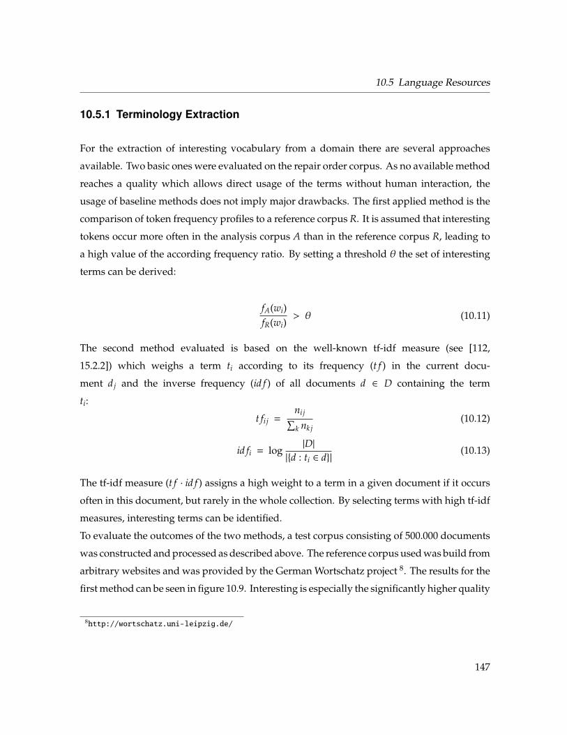
10.5 Language Resources
10.5.1 Terminology Extraction
For the extraction of interesting vocabulary from a domain there are several approaches
available. Two basic ones were evaluated on the repair order corpus. As no available method
reaches a quality which allows direct usage of the terms without human interaction, the
usage of baseline methods does not imply major drawbacks. The first applied method is the
comparison of token frequency profiles to a reference corpus R. It is assumed that interesting
tokens occur more often in the analysis corpus A than in the reference corpus R, leading to
a high value of the according frequency ratio. By setting a threshold θ the set of interesting
terms can be derived:
fA(wi)fR(wi)
> θ (10.11)
The second method evaluated is based on the well-known tf-idf measure (see [112,
15.2.2]) which weighs a term ti according to its frequency (t f ) in the current docu-
ment d j and the inverse frequency (id f ) of all documents d ∈ D containing the term
ti:
t fi j =ni j∑k nkj
(10.12)
id fi = log|D|
|{d : ti ∈ d}|(10.13)
The tf-idf measure (t f · id f ) assigns a high weight to a term in a given document if it occurs
often in this document, but rarely in the whole collection. By selecting terms with high tf-idf
measures, interesting terms can be identified.
To evaluate the outcomes of the two methods, a test corpus consisting of 500.000 documents
was constructed and processed as described above. The reference corpus used was build from
arbitrary websites and was provided by the German Wortschatz project 8. The results for the
first method can be seen in figure 10.9. Interesting is especially the significantly higher quality
8http://wortschatz.uni-leipzig.de/
147
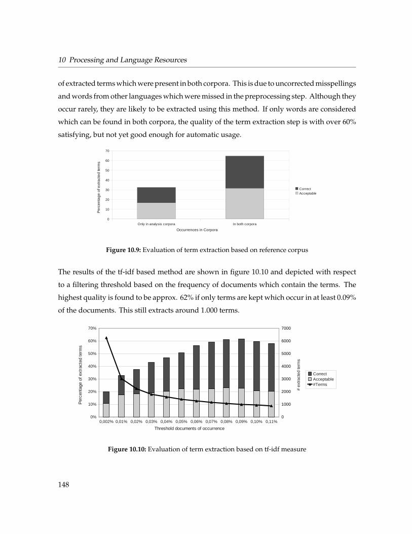
10 Processing and Language Resources
of extracted terms which were present in both corpora. This is due to uncorrected misspellings
and words from other languages which were missed in the preprocessing step. Although they
occur rarely, they are likely to be extracted using this method. If only words are considered
which can be found in both corpora, the quality of the term extraction step is with over 60%
satisfying, but not yet good enough for automatic usage.
Only in analysis corpora In both corpora
0
10
20
30
40
50
60
70
CorrectAcceptable
Occurrences in Corpora
Pe
rce
nta
ge
of e
xtra
cte
d te
rms
Figure 10.9: Evaluation of term extraction based on reference corpus
The results of the tf-idf based method are shown in figure 10.10 and depicted with respect
to a filtering threshold based on the frequency of documents which contain the terms. The
highest quality is found to be approx. 62% if only terms are kept which occur in at least 0.09%
of the documents. This still extracts around 1.000 terms.
0,002% 0,01% 0,02% 0,03% 0,04% 0,05% 0,06% 0,07% 0,08% 0,09% 0,10% 0,11%0%
10%
20%
30%
40%
50%
60%
70%
0
1000
2000
3000
4000
5000
6000
7000
CorrectAcceptable#Terms
Threshold documents of occurrence
Per
cent
age
of e
xtra
c ted
ter
ms
# e
xtra
cte
d te
rms
Figure 10.10: Evaluation of term extraction based on tf-idf measure
148
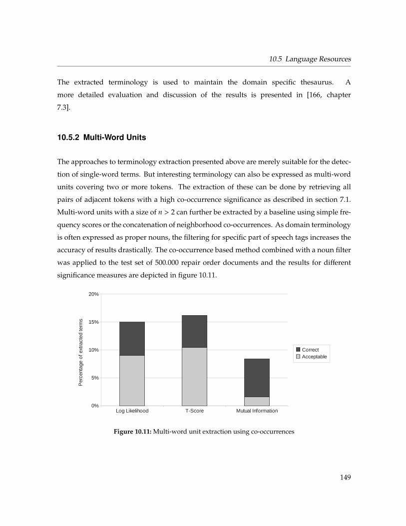
10.5 Language Resources
The extracted terminology is used to maintain the domain specific thesaurus. A
more detailed evaluation and discussion of the results is presented in [166, chapter
7.3].
10.5.2 Multi-Word Units
The approaches to terminology extraction presented above are merely suitable for the detec-
tion of single-word terms. But interesting terminology can also be expressed as multi-word
units covering two or more tokens. The extraction of these can be done by retrieving all
pairs of adjacent tokens with a high co-occurrence significance as described in section 7.1.
Multi-word units with a size of n > 2 can further be extracted by a baseline using simple fre-
quency scores or the concatenation of neighborhood co-occurrences. As domain terminology
is often expressed as proper nouns, the filtering for specific part of speech tags increases the
accuracy of results drastically. The co-occurrence based method combined with a noun filter
was applied to the test set of 500.000 repair order documents and the results for different
significance measures are depicted in figure 10.11.
Log Likelihood T-Score Mutual Information0%
5%
10%
15%
20%
CorrectAcceptable
Per
cent
a ge
of
e xtr
acte
d te
rms
Figure 10.11: Multi-word unit extraction using co-occurrences
149
10 Processing and Language Resources
The results show that only a small amount of relevant multi-word units is extracted by the
approach. Although the method extracts a much higher amount of interesting units, most of
them are unfortunately without relevance for the domain. The method can however be used
to support a human knowledge engineer by maintaining the domain specific thesaurus. A
more exhaustive overview over the experiments and further details of the evaluations can be
found in [166, chapter 7.3.3].
10.5.3 Domain Thesaurus
Many methods used in information extraction are based on or can at least take advantage
of a thesaurus as described in section 7.3. Even if more advanced relations like hyponomy
or meronymy are left aside, basic relations like synonymy provide crucial means for pattern
matching and text similarity. Although the creation of a comprehensive thesaurus may be
infeasible for a given task, it makes sense to create synonym lists and other useful resources
always in a format offering hierarchical structure, attributes and relations. As already existing
thesauri do not cover automotive domain vocabulary and the enrichment of existing resources
like WordNet 9 (see [120]) is error prone and time consuming, a domain specific thesaurus was
designed and implemented. Another advantage of defining a specialized lexical knowledge
base was the addition of matching specific information, which is neglected in commonly
used thesauri. For the task of repair order text processing, several distinct requirements were
identified:
1. The handling of synonyms can be seen as a basic, but crucial task. One concept may be
expressed in different ways, but it is necessary to identify all these different expressions
as the same concept. With respect to the automotive domain, the words car and vehicle
should be treated as synonyms as well as for example wiring and cabling.
2. Identical words may refer to different concepts (ambiguities like homonyms), which
makes it necessary to disambiguate the word sense. Homonyms may exist within the
9http://wordnet.princeton.edu/
150
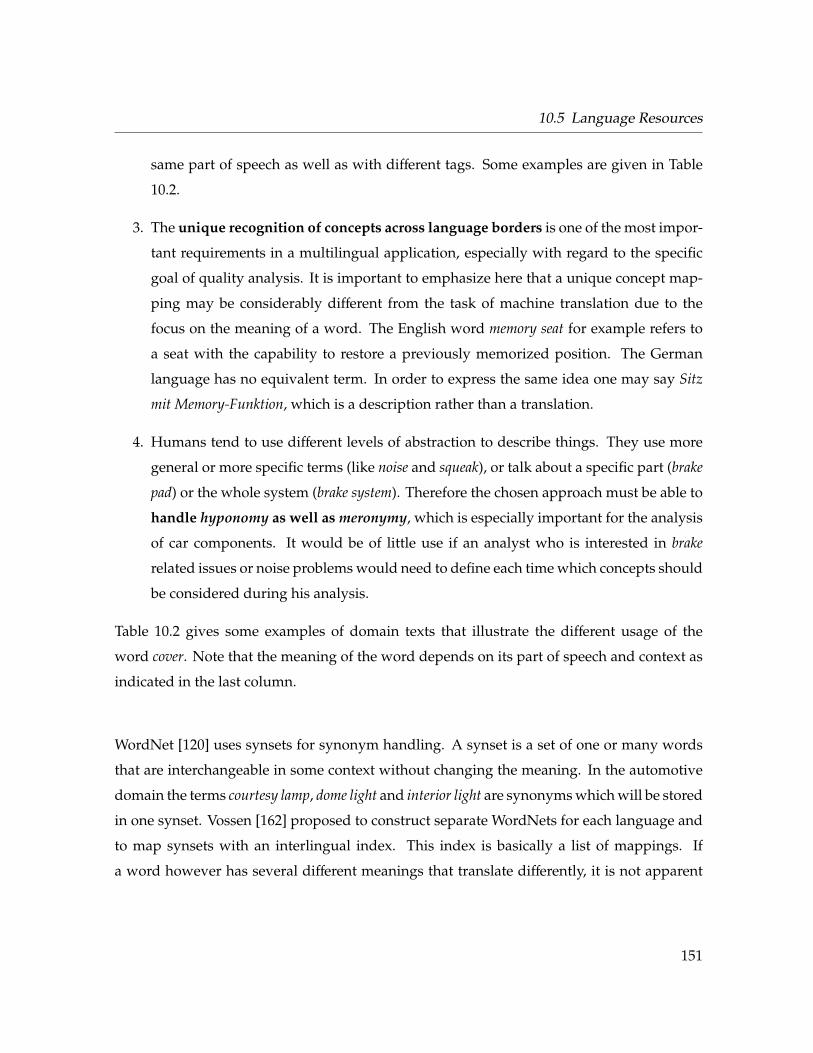
10.5 Language Resources
same part of speech as well as with different tags. Some examples are given in Table
10.2.
3. The unique recognition of concepts across language borders is one of the most impor-
tant requirements in a multilingual application, especially with regard to the specific
goal of quality analysis. It is important to emphasize here that a unique concept map-
ping may be considerably different from the task of machine translation due to the
focus on the meaning of a word. The English word memory seat for example refers to
a seat with the capability to restore a previously memorized position. The German
language has no equivalent term. In order to express the same idea one may say Sitz
mit Memory-Funktion, which is a description rather than a translation.
4. Humans tend to use different levels of abstraction to describe things. They use more
general or more specific terms (like noise and squeak), or talk about a specific part (brake
pad) or the whole system (brake system). Therefore the chosen approach must be able to
handle hyponomy as well as meronymy, which is especially important for the analysis
of car components. It would be of little use if an analyst who is interested in brake
related issues or noise problems would need to define each time which concepts should
be considered during his analysis.
Table 10.2 gives some examples of domain texts that illustrate the different usage of the
word cover. Note that the meaning of the word depends on its part of speech and context as
indicated in the last column.
WordNet [120] uses synsets for synonym handling. A synset is a set of one or many words
that are interchangeable in some context without changing the meaning. In the automotive
domain the terms courtesy lamp, dome light and interior light are synonyms which will be stored
in one synset. Vossen [162] proposed to construct separate WordNets for each language and
to map synsets with an interlingual index. This index is basically a list of mappings. If
a word however has several different meanings that translate differently, it is not apparent
151
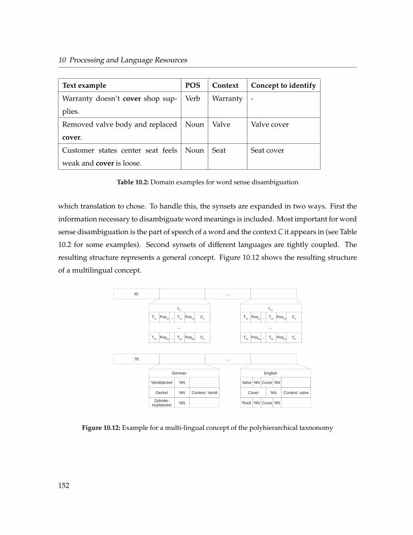
10 Processing and Language Resources
Text example POS Context Concept to identify
Warranty doesn’t cover shop sup-
plies.
Verb Warranty -
Removed valve body and replaced
cover.
Noun Valve Valve cover
Customer states center seat feels
weak and cover is loose.
Noun Seat Seat cover
Table 10.2: Domain examples for word sense disambiguation
which translation to chose. To handle this, the synsets are expanded in two ways. First the
information necessary to disambiguate word meanings is included. Most important for word
sense disambiguation is the part of speech of a word and the context C it appears in (see Table
10.2 for some examples). Second synsets of different languages are tightly coupled. The
resulting structure represents a general concept. Figure 10.12 shows the resulting structure
of a multilingual concept.
ID ....
T11
C1
L1
...
Lm
...
78 ....
Ventildeckel NN
German
Deckel NN Context: Ventil
English
Cover
Valve
Pos11
T1n
Pos1n..
Tk1
Ck
Posk1
Tkn
Poskn..
T11
C1
Pos11
T1n
Pos1n..
Tk1
Ck
Posk1
Tkn
Poskn..
NN
NN
Context: valve
Zylinder-kopfdeckel NN
CoverNN
Rock NNCoverNN
Figure 10.12: Example for a multi-lingual concept of the polyhierarchical taxnonomy
152
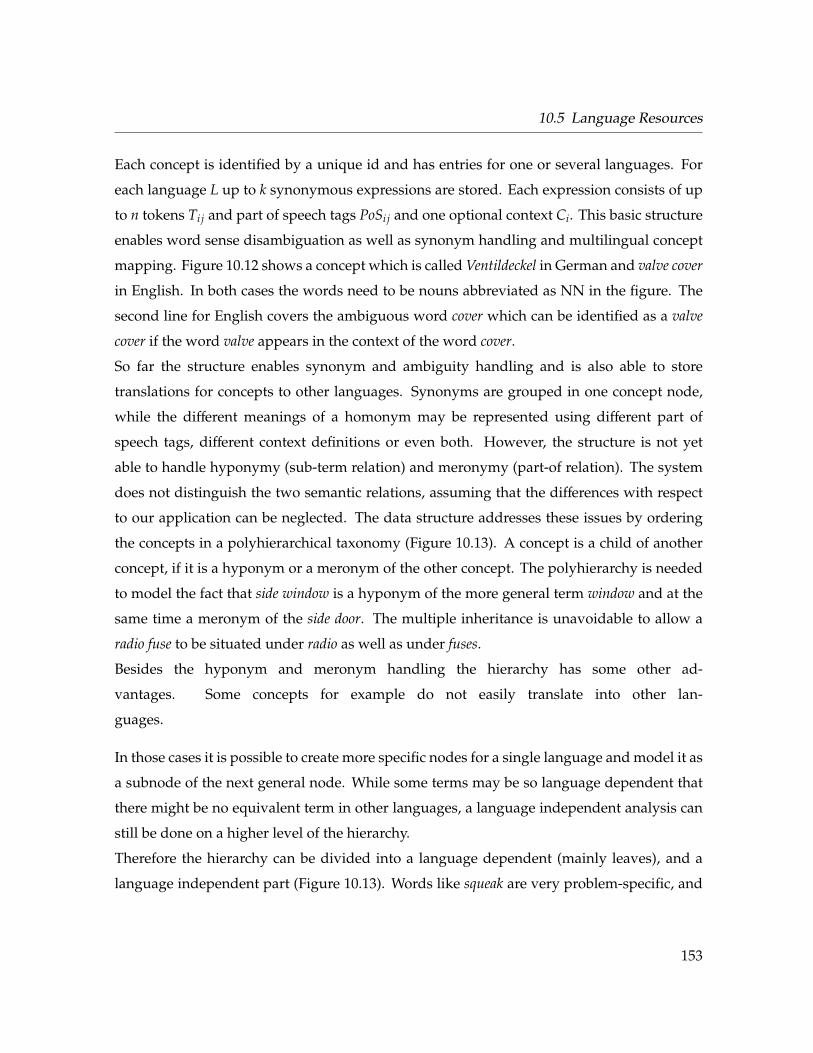
10.5 Language Resources
Each concept is identified by a unique id and has entries for one or several languages. For
each language L up to k synonymous expressions are stored. Each expression consists of up
to n tokens Ti j and part of speech tags PoSi j and one optional context Ci. This basic structure
enables word sense disambiguation as well as synonym handling and multilingual concept
mapping. Figure 10.12 shows a concept which is called Ventildeckel in German and valve cover
in English. In both cases the words need to be nouns abbreviated as NN in the figure. The
second line for English covers the ambiguous word cover which can be identified as a valve
cover if the word valve appears in the context of the word cover.
So far the structure enables synonym and ambiguity handling and is also able to store
translations for concepts to other languages. Synonyms are grouped in one concept node,
while the different meanings of a homonym may be represented using different part of
speech tags, different context definitions or even both. However, the structure is not yet
able to handle hyponymy (sub-term relation) and meronymy (part-of relation). The system
does not distinguish the two semantic relations, assuming that the differences with respect
to our application can be neglected. The data structure addresses these issues by ordering
the concepts in a polyhierarchical taxonomy (Figure 10.13). A concept is a child of another
concept, if it is a hyponym or a meronym of the other concept. The polyhierarchy is needed
to model the fact that side window is a hyponym of the more general term window and at the
same time a meronym of the side door. The multiple inheritance is unavoidable to allow a
radio fuse to be situated under radio as well as under fuses.
Besides the hyponym and meronym handling the hierarchy has some other ad-
vantages. Some concepts for example do not easily translate into other lan-
guages.
In those cases it is possible to create more specific nodes for a single language and model it as
a subnode of the next general node. While some terms may be so language dependent that
there might be no equivalent term in other languages, a language independent analysis can
still be done on a higher level of the hierarchy.
Therefore the hierarchy can be divided into a language dependent (mainly leaves), and a
language independent part (Figure 10.13). Words like squeak are very problem-specific, and
153
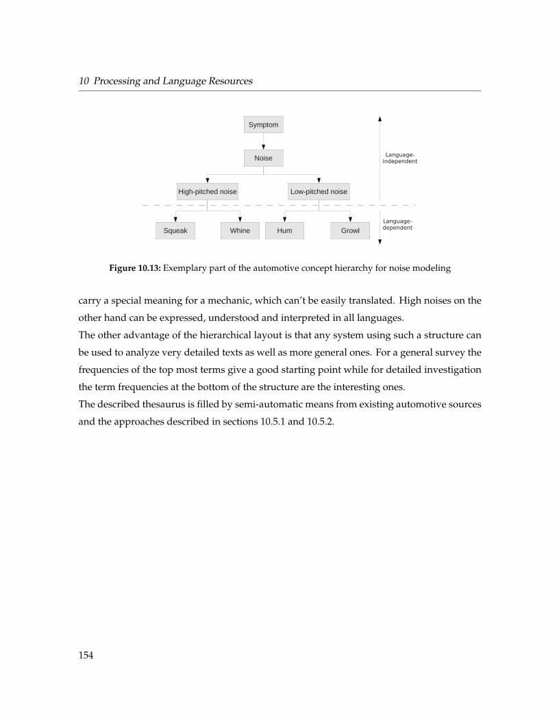
10 Processing and Language Resources
Symptom
Noise
High-pitched noise Low-pitched noise
Squeak Whine GrowlHum
Language-independent
Language-dependent
Figure 10.13: Exemplary part of the automotive concept hierarchy for noise modeling
carry a special meaning for a mechanic, which can’t be easily translated. High noises on the
other hand can be expressed, understood and interpreted in all languages.
The other advantage of the hierarchical layout is that any system using such a structure can
be used to analyze very detailed texts as well as more general ones. For a general survey the
frequencies of the top most terms give a good starting point while for detailed investigation
the term frequencies at the bottom of the structure are the interesting ones.
The described thesaurus is filled by semi-automatic means from existing automotive sources
and the approaches described in sections 10.5.1 and 10.5.2.
154
10.6 Concept Recognition
10.6 Concept Recognition
As described in chapter 9 the interesting entities for the automotive quality domain are given
by a set of car components and their corresponding problems or failures, expressed as verbs
and adjectives. This is a crucial difference to existing named entity recognition systems,
which try to find an open class of proper nouns. The components of a car can be exhaustively
enumerated, and even the symptoms can be covered to a great extent using lists. And even
if the consideration of symptoms as an open class would be of interest, the subsequent use
for structured reporting and data mining can be doubted. With respect to the current state
of the art it would be impossible to automatically assign them to the right categories or even
map them to suitable synonyms. Therefore a dictionary based approach seems to be sensible
and is implemented using the thesaurus described in section 10.5.3.
10.6.1 Taxonomy Expansion
Before the matching takes place, a taxonomy expansion step is applied, which is further
divided into synonym expansion and context expansion. For the synonym expansion of a
term ti, the taxonomy is searched for a term t j (with synonyms) such that a token-delimited
substring s ≤ ti is one of the synonyms of t j. Then the synset ti is expanded by creating
new synonyms and replacing the substring s from ti with all synonyms of t j. If there are for
example the two synsets s1 = (light, lamp) and s2 = (fog light), s2 can be expanded to s′2 = (fog
light, fog lamp). Special attention must be paid to the context while substituting s with the
synonyms of s defined in t j. The substitution may only be done if both ti and t j require no or
the same context.
It is important to be aware of the fact that this step may lead to synonyms which are not
common, but it is very unlikely to create synonyms which are erroneous. Similar to the
synonym expansion, a context expansion step is performed by adding all alternative con-
texts that can be obtained by replacing each word in the context with its synonyms defined
155
10 Processing and Language Resources
elsewhere in the taxonomy. The additional synonyms created during the expansion are
not stored in the taxonomy, they are only derived at runtime. These two expansion steps
reduce the amount of information that needs to be entered manually by an expert signifi-
cantly.
10.6.2 Matching Process
For an efficient processing a separate trie is built for every language defined in the taxonomy,
containing all synonyms of all synsets of the language, with one token per node. The separate
construction of a trie for each language has the additional advantage that only the information
for the languages currently used needs to be loaded into memory. This trie can be efficiently
queried to find the matching concepts in the input text. If a sequence of 1 to n tokens
t1...tn matches a concept, the sequence of part of speech annotations associated with t1...tn is
compared with the sequence of part of speech tags for all tokens of the concept. Besides the
part of speech constraint, the matcher checks the context on both sides. If several concepts
match a given input, but they all require a different context, the matcher will choose the
concept for which the distance between the sequence of matching tokens and the required
context is minimal. If no such context can be found within a distance limited by some
threshold θ, the matcher will choose a concept that requires no context (if available) or will
return no match for the input sequence. This choice is a good approximation, as a concept
without a defined context is more general, than a similar one with context. The threshold may
reduce the recall, but ensures a high precision even if no sentence boundaries are available.
Note that there may be several potential matches for a given input sequence, which is in fact
a common situation. Potential strategies for the list of matches include an enumeration of all
matches or the longest match. In this case the latter was chosen. Potential matches for the
input sequence seat cover may for example include seat, cover and seat cover, of which only seat
cover is considered to be an appropriate match.
156
10.6 Concept Recognition
10.6.3 Evaluation of Concept Recognition
The knowledge base used for the experimental evaluation was constructed using automated
imports from company sources (technical dictionaries, component hierarchies) and approxi-
mately four weeks of manual work. It contains around 2.000 concepts with synonyms, part
of speech tags and context hints. Although most of the concepts are specified in several
languages (at least German and English), only the English definitions have been thoroughly
tested. To reduce the evaluation effort, the system is only evaluated for English data. As
the multilingual capabilities are accomplished by the knowledge-base structure itself and are
just as good as the information maintained in it, the English evaluation on entity recognition
and word sense disambiguation is representative. The evaluation uses the recall and precision
measures as defined in [112, chapter 8.1], which are commonly used for text mining tasks.
To examine the word sense disambiguation performance of the system, 100 concepts which
were disambiguated using pos-tags were manually reviewed. Another 100 concepts were
disambiguated using context keywords and also manually reviewed. The part of speech tags
were obtained by a Hidden-Markov-Model based part of speech tagger (Hammer10), which
was trained on approx. 26.000 manually annotated words from our domain and yields an
accuracy of 92.2%. Both approaches achieved good results: The part of speech based disam-
biguation showed an accuracy of 91%, the context based evaluation an accuracy of 92%. In
contrast to that, a simple baseline method using always the most frequent meaning was eval-
uated. The baseline showed an accuracy of 82% related to part of speech based ambiguities,
and an accuracy of 52% for the context-based ambiguities, which is significantly worse.
Figure 10.14 shows an evaluation for the word sense disambiguation using the context. The
word band is disambiguated using its context to distinguish its different meanings am band,
fm band and radio band for the more general concept. The figure shows that best results in
terms of the F-measure are achieved with a context size of approx. 5 words, which slightly
differs from other concepts. At first glance it may be surprising that a larger context can
actually decrease the performance as intuitively a larger context provides more information
10http://www.vf.utwente.nl/˜infrieks/stt/stt.html
157
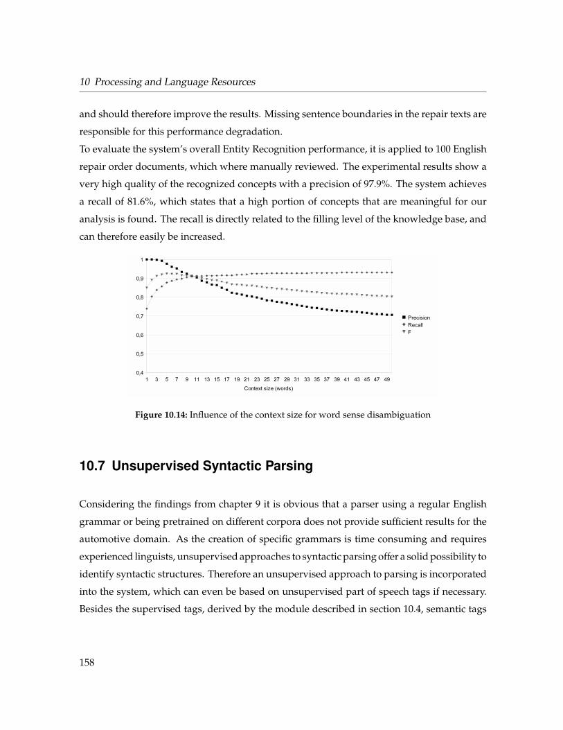
10 Processing and Language Resources
and should therefore improve the results. Missing sentence boundaries in the repair texts are
responsible for this performance degradation.
To evaluate the system’s overall Entity Recognition performance, it is applied to 100 English
repair order documents, which where manually reviewed. The experimental results show a
very high quality of the recognized concepts with a precision of 97.9%. The system achieves
a recall of 81.6%, which states that a high portion of concepts that are meaningful for our
analysis is found. The recall is directly related to the filling level of the knowledge base, and
can therefore easily be increased.
Figure 10.14: Influence of the context size for word sense disambiguation
10.7 Unsupervised Syntactic Parsing
Considering the findings from chapter 9 it is obvious that a parser using a regular English
grammar or being pretrained on different corpora does not provide sufficient results for the
automotive domain. As the creation of specific grammars is time consuming and requires
experienced linguists, unsupervised approaches to syntactic parsing offer a solid possibility to
identify syntactic structures. Therefore an unsupervised approach to parsing is incorporated
into the system, which can even be based on unsupervised part of speech tags if necessary.
Besides the supervised tags, derived by the module described in section 10.4, semantic tags
158
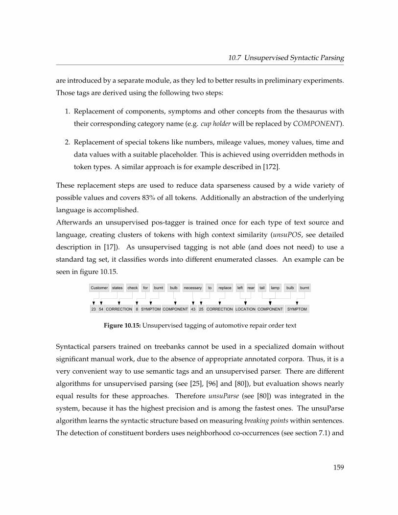
10.7 Unsupervised Syntactic Parsing
are introduced by a separate module, as they led to better results in preliminary experiments.
Those tags are derived using the following two steps:
1. Replacement of components, symptoms and other concepts from the thesaurus with
their corresponding category name (e.g. cup holder will be replaced by COMPONENT).
2. Replacement of special tokens like numbers, mileage values, money values, time and
data values with a suitable placeholder. This is achieved using overridden methods in
token types. A similar approach is for example described in [172].
These replacement steps are used to reduce data sparseness caused by a wide variety of
possible values and covers 83% of all tokens. Additionally an abstraction of the underlying
language is accomplished.
Afterwards an unsupervised pos-tagger is trained once for each type of text source and
language, creating clusters of tokens with high context similarity (unsuPOS, see detailed
description in [17]). As unsupervised tagging is not able (and does not need) to use a
standard tag set, it classifies words into different enumerated classes. An example can be
seen in figure 10.15.
Figure 10.15: Unsupervised tagging of automotive repair order text
Syntactical parsers trained on treebanks cannot be used in a specialized domain without
significant manual work, due to the absence of appropriate annotated corpora. Thus, it is a
very convenient way to use semantic tags and an unsupervised parser. There are different
algorithms for unsupervised parsing (see [25], [96] and [80]), but evaluation shows nearly
equal results for these approaches. Therefore unsuParse (see [80]) was integrated in the
system, because it has the highest precision and is among the fastest ones. The unsuParse
algorithm learns the syntactic structure based on measuring breaking points within sentences.
The detection of constituent borders uses neighborhood co-occurrences (see section 7.1) and
159
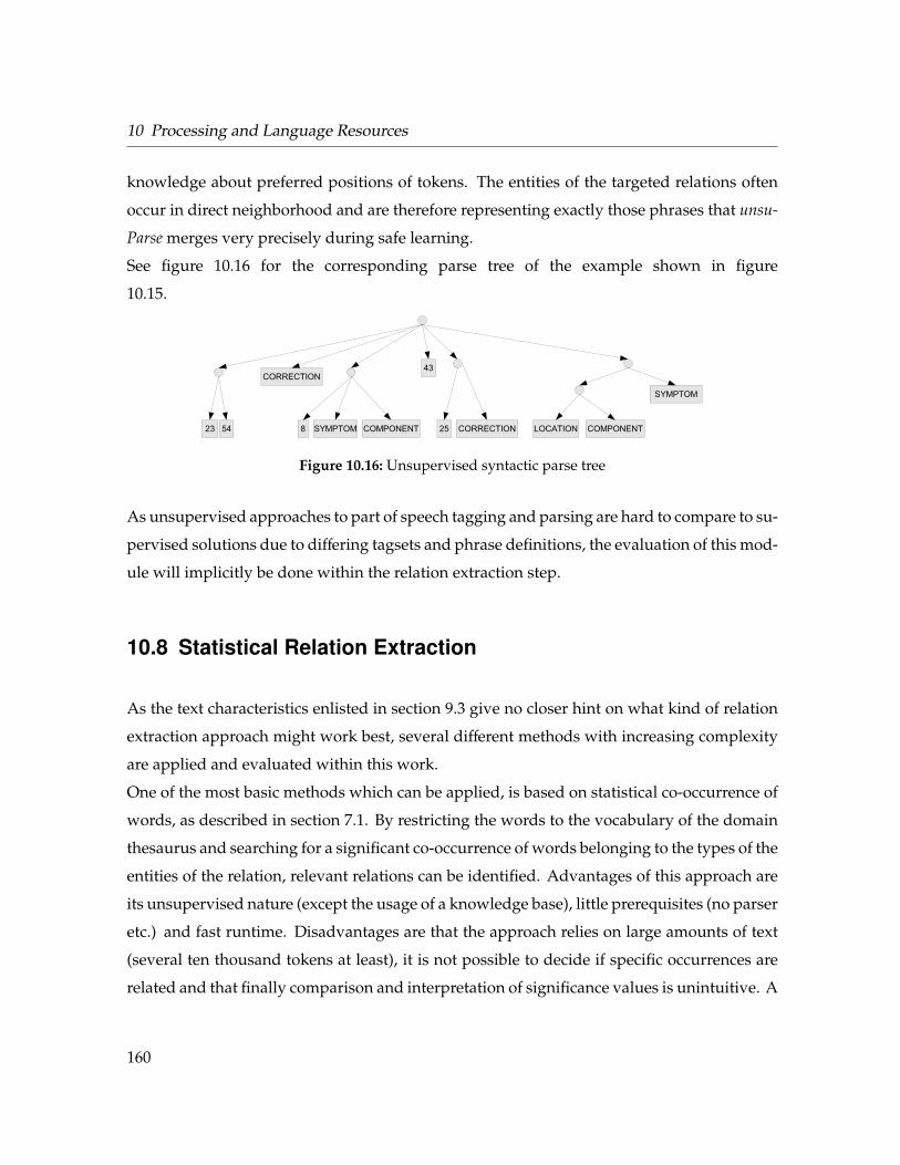
10 Processing and Language Resources
knowledge about preferred positions of tokens. The entities of the targeted relations often
occur in direct neighborhood and are therefore representing exactly those phrases that unsu-
Parse merges very precisely during safe learning.
See figure 10.16 for the corresponding parse tree of the example shown in figure
10.15.
Figure 10.16: Unsupervised syntactic parse tree
As unsupervised approaches to part of speech tagging and parsing are hard to compare to su-
pervised solutions due to differing tagsets and phrase definitions, the evaluation of this mod-
ule will implicitly be done within the relation extraction step.
10.8 Statistical Relation Extraction
As the text characteristics enlisted in section 9.3 give no closer hint on what kind of relation
extraction approach might work best, several different methods with increasing complexity
are applied and evaluated within this work.
One of the most basic methods which can be applied, is based on statistical co-occurrence of
words, as described in section 7.1. By restricting the words to the vocabulary of the domain
thesaurus and searching for a significant co-occurrence of words belonging to the types of the
entities of the relation, relevant relations can be identified. Advantages of this approach are
its unsupervised nature (except the usage of a knowledge base), little prerequisites (no parser
etc.) and fast runtime. Disadvantages are that the approach relies on large amounts of text
(several ten thousand tokens at least), it is not possible to decide if specific occurrences are
related and that finally comparison and interpretation of significance values is unintuitive. A
160
10.8 Statistical Relation Extraction
quality advocate interested in how many instances of a specific problem occurred, may have
problems with comparisons based on significance levels. Although the method is therefore
inherently less useful for the domain, it is implemented and evaluated first, due to the ease
of application. To make the results more meaningful, several different kinds of relations are
detected in parallel and are visualized as graphs of clusters.
10.8.1 Workflow
The approach can be divided into several steps of a more complex UIMA workflow, which
is outlined below.
Input to the workflow is a set of multidimensional data points S = {x1, .., xn} with xi ∈ Fd,
representing the structured (nominal scaled) data with their values in a d-dimensional
feature space, and a set of text documents T = t1, .., tn in (potentially different) lan-
guages with a bijective function f (xi) � ti, mapping one text document to every data
point.
1. The document collection T is transfered into a cleaned text collection T′ by preprocessing
every document ti ∈ T to a document t′i ∈ T′with improved textual quality (see sections
10.1 to 10.3).
2. By applying the thesaurus based matcher (see section 10.6), a set of language indepen-
dent concepts Ci = {c1, ..., cn} can be extracted from each document t′i . Synonyms as
well as homonyms are resolved using the thesaurus.
3. The extracted concepts are combined with the structured data S, leading to the data set
S′ = {x′1, .., x′n}. The feature space is extended by the concepts in the taxonomy, and is
now F′.
4. Co-occurrence significances for every pair of concepts are calculated. The t-Score is used
as a significance measure (see section 7.1), as it seemed most reasonable with respect to
161
10 Processing and Language Resources
our application and showed superior performance in prior experiments. Measures like
the Dice coefficient or the Jaccard coefficient were discarded, because they tend to score
co-occurrences down, when one of the two measured items occurs rarely, and the other
one is frequent (cp. [32]). Mutual Information was also discarded, because it tends
to prefer seldom events (in contrast to the Local Mutual Information, which behaves
similar to the t-Score). These properties are inappropriate with regard to the task of
quality analysis. Interesting here are especially frequent events, but without ignoring
seldom events, which might be used as an indicator for early warning.
5. The application of the significance measure with a filtering threshold θ leads to a set of
significant co-occurring items, which can also be written as a matrix CM, with
CMi, j =
Sig(F′i ,F′
j), if Sig(F′i ,F′
j) > θ,
0 else(10.14)
6. This matrix CM can be read as an adjacency matrix of a graph and is used as input for
a graph clustering algorithm, which creates a clustering C = {C1, ...,Cn} of the feature
space, grouping items which significantly occur together. These clusters contain the
structured items, as well as the items of the taxonomy obtained from the analysis of the
textual data (section 10.8.3). Graph clustering is well known for all applications which
are not based on data vectors, but rather on a similarity (or distance) matrix between
arbitrary objects. Overviews can be found in [56], [28] and [18]. The clustering of word
co-occurrence graphs suggests itself. Approaches are described in [16] or [115], but are
based on words instead of extracted concepts of a taxonomy.
7. The last step of the workflow is the visualization of the results using a graph layout
algorithm.
162
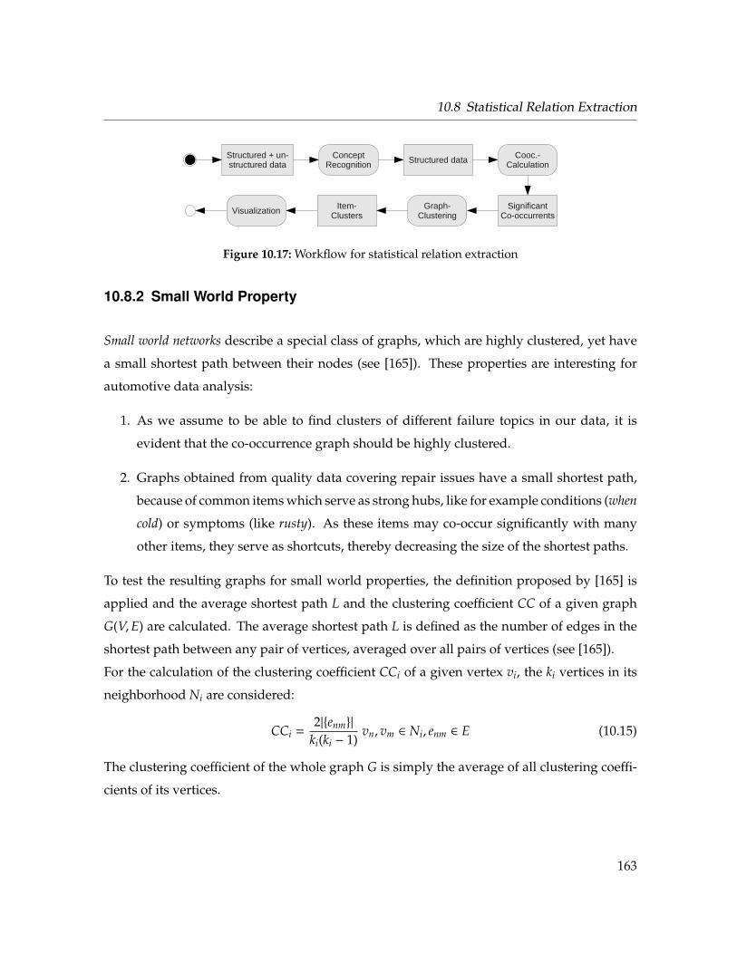
10.8 Statistical Relation Extraction
Structured + un-structured data
ConceptRecognition
Structured data
SignificantCo-occurrents
Cooc.-Calculation
Graph-Clustering
Item-Clusters
Visualization
Figure 10.17: Workflow for statistical relation extraction
10.8.2 Small World Property
Small world networks describe a special class of graphs, which are highly clustered, yet have
a small shortest path between their nodes (see [165]). These properties are interesting for
automotive data analysis:
1. As we assume to be able to find clusters of different failure topics in our data, it is
evident that the co-occurrence graph should be highly clustered.
2. Graphs obtained from quality data covering repair issues have a small shortest path,
because of common items which serve as strong hubs, like for example conditions (when
cold) or symptoms (like rusty). As these items may co-occur significantly with many
other items, they serve as shortcuts, thereby decreasing the size of the shortest paths.
To test the resulting graphs for small world properties, the definition proposed by [165] is
applied and the average shortest path L and the clustering coefficient CC of a given graph
G(V,E) are calculated. The average shortest path L is defined as the number of edges in the
shortest path between any pair of vertices, averaged over all pairs of vertices (see [165]).
For the calculation of the clustering coefficient CCi of a given vertex vi, the ki vertices in its
neighborhood Ni are considered:
CCi =2|{enm}|
ki(ki − 1)vn, vm ∈ Ni, enm ∈ E (10.15)
The clustering coefficient of the whole graph G is simply the average of all clustering coeffi-
cients of its vertices.
163
10 Processing and Language Resources
A given graph G is said to be small world, if its values for L are nearly as small as in a ran-
dom graph Grandom but its clustering coefficient is remarkably higher, similar to a completely
ordered graph Gordered (e.g. a ring lattice).
10.8.3 Graph Clustering
Graph Clustering tries to break a given graph into meaningful subgraphs, normally so that the
vertices in the subgraphs are strongly connected to each other, yet having only few edges to
other subgraphs (or edges with high weights within the subgraphs, and few edges with small
weights to other subgraphs). Although some vector clustering algorithms can be applied for
graphs, there is also a set of graph clustering algorithms, which normally use methods and
ideas from graph theory, like the minimum cut or minimal spanning trees, to find clusters in
a graph.
In order to find general problem groups in the co-occurrence graph of our data, three parti-
tional graph clustering algorithms are applied and evaluated. These algorithms were chosen
because they have only few (or none) parameters, and find the number of clusters automat-
ically. The stochastic transition matrix, where the edge weights of a node sum up to one, is
used as input for all algorithms. This is important to devalue hubs, which could otherwise
glue the graph together.
10.8.4 Markov Cluster Algorithm
The Markov Cluster Algorithm (or MCL algorithm) is based on the idea of performing a random
walk on the graph (see [161]). A random walk which once entered a dense area in the graph,
will most probably visit most of the vertices of the dense area before leaving it. This idea
is realized by computing flows in the graph, which can be done by iteratively applying two
operations
164
10.8 Statistical Relation Extraction
1. The expansion step, which computes the power of the transition matrix, thereby simu-
lating random walks.
2. The inflation step, which sets the matrix to the Hadamard power (to strengthen strong
flows, and to devalue weak flows by taking the power of each matrix entry), and then
re-normalizing it back to a stochastic transition matrix.
The advantage of this algorithm is found in its deterministic behavior, therefore always
creating the same clustering of a given graph. Unfortunately the algorithm isn’t very fast,
having a runtime complexity of O(n3). Although the author describes possible optimiza-
tions of his algorithm (see [161]), e.g. by pruning edges, the base algorithm is used in this
work.
10.8.5 Chinese Whispers
The Chinese Whispers algorithm is a very basic algorithm, which can be seen as a special
version of the MCL algorithm, yet being more efficient (O(|E|), which is especially fine for
sparse graphs) and parameter-free (see [18]).
After initially assigning each vertex in the graph a different class label, the algorithm itera-
tively visits through all vertices in a randomized order, and assign each vertex the predomi-
nant class label in its neighborhood. The algorithm stops after a small amount of iterations,
or if convergence is reached. The drawback of this algorithm is its randomized and indeter-
ministic behavior.
10.8.6 Geometric MST Clustering
The Geometric MST Clustering (or GMC algorithm) is an algorithm which combines spectral
partitioning with geometric clustering (see [28]). It calculates the eigenvalues and eigen-
vectors from the normalized adjacency matrix (the stochastic transition matrix) and uses a
small number d of them to reweight the edges of the graph. After this step a minimum
165
10 Processing and Language Resources
spanning tree is created, and the clustering is created by pruning edges of the MST. All possi-
bilities (thresholds) for pruning edges are explored while trying to maximize a given quality
measure.
10.8.7 Evaluation and Experimental Results
To measure the quality of a clustering C, two quality measures based on graph theory are
applied. An overview of possible measures is given in [28].
The first quality measure used is called performance. It counts the number of correctly inter-
preted node pairs. This is done by taking the sum of intra-cluster edges and non-adjacent
nodes in different clusters, and normalizing it with the sum of all pairs of nodes. The measure
was reformulated for weighted graphs, by using the sum of intra-cluster edge weights m(C)
and by multiplying the sum of non-adjacent nodes and the sum of all pairs of nodes with the
average edge weight a(G).
Performance(C) =m(C) + a(G)
∑{v,w}<E,v∈Ci,w∈C j,i, j
a(G)0.5n(n − 1)(10.16)
The second measure is the coverage of a clustering, which is calculated as the ratio between
intra-cluster edge weights m(C) and the weights of all edges:
Coverage(C) =m(C)∑
ei j∈E w(ei j)(10.17)
As coverage prefers clusterings with a small number of clusters (the maximum is reached
for one single cluster), a changed formula is used, which prefers clusterings with more
clusters:
Coverage(C) = log (|C|)m(C)∑
ei j∈E w(ei j)(10.18)
The data used for the experiments is a dataset with approximately 10.000 repairs from the
automotive domain, including model, model year and repair order text. The texts are pre-
processed as described in sections 10.1 to 10.3 and symptom descriptions, component names
166
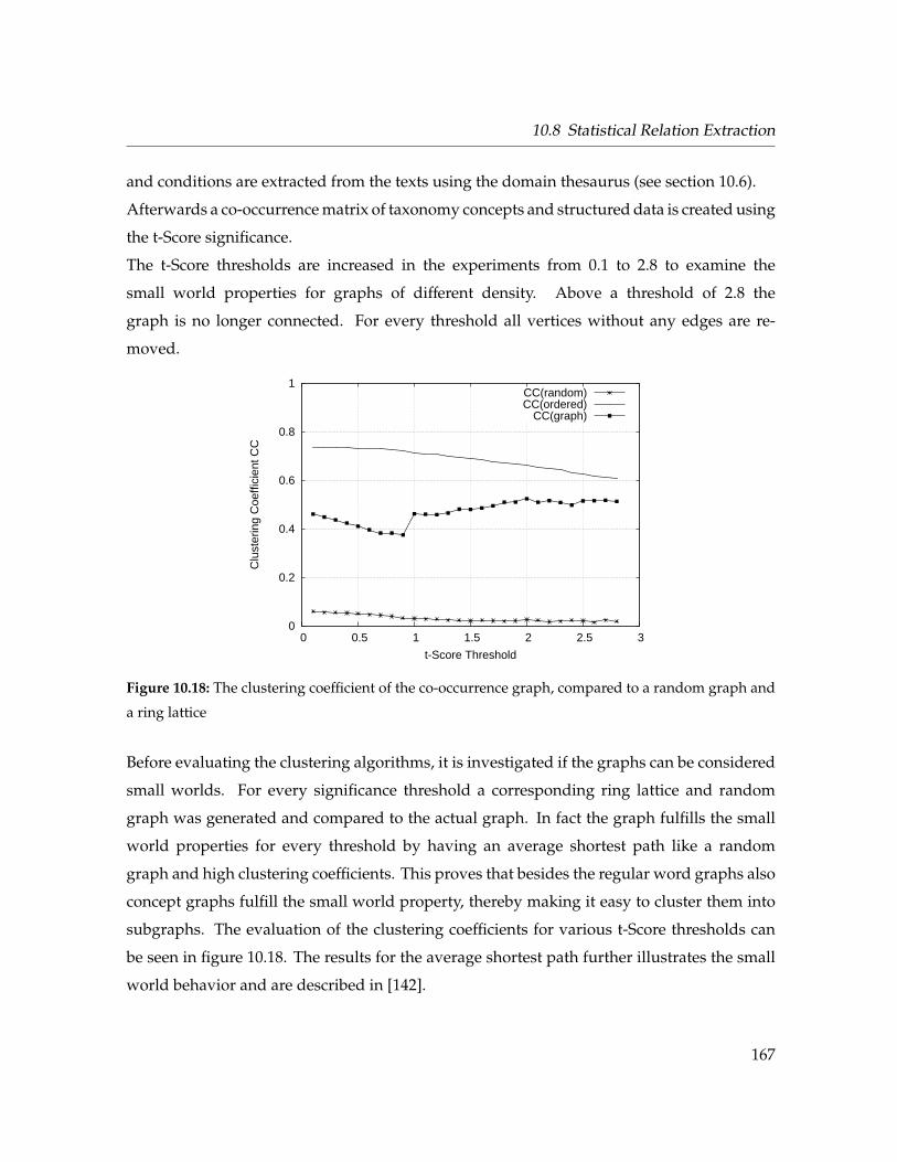
10.8 Statistical Relation Extraction
and conditions are extracted from the texts using the domain thesaurus (see section 10.6).
Afterwards a co-occurrence matrix of taxonomy concepts and structured data is created using
the t-Score significance.
The t-Score thresholds are increased in the experiments from 0.1 to 2.8 to examine the
small world properties for graphs of different density. Above a threshold of 2.8 the
graph is no longer connected. For every threshold all vertices without any edges are re-
moved.
0
0.2
0.4
0.6
0.8
1
0 0.5 1 1.5 2 2.5 3
Clu
ster
ing
Coe
ffici
ent C
C
t-Score Threshold
CC(random)CC(ordered)
CC(graph)
Figure 10.18: The clustering coefficient of the co-occurrence graph, compared to a random graph and
a ring lattice
Before evaluating the clustering algorithms, it is investigated if the graphs can be considered
small worlds. For every significance threshold a corresponding ring lattice and random
graph was generated and compared to the actual graph. In fact the graph fulfills the small
world properties for every threshold by having an average shortest path like a random
graph and high clustering coefficients. This proves that besides the regular word graphs also
concept graphs fulfill the small world property, thereby making it easy to cluster them into
subgraphs. The evaluation of the clustering coefficients for various t-Score thresholds can
be seen in figure 10.18. The results for the average shortest path further illustrates the small
world behavior and are described in [142].
167
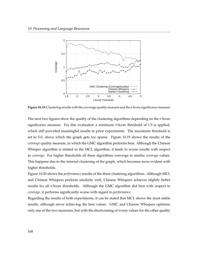
10 Processing and Language Resources
0
0.5
1
1.5
2
1.5 2 2.5 3 3.5 4 4.5 5
Cov
erag
e
t-Score Threshold
GMC-Clustering (CoverageQuality)Chinese WhispersMarkov Clustering
Figure 10.19: Clustering results with the coverage quality measure and the t-Score significance measure
The next two figures show the quality of the clustering algorithms depending on the t-Score
significance measure. For this evaluation a minimum t-Score threshold of 1.5 is applied,
which still provided meaningful results in prior experiments. The maximum threshold is
set to 5.0, above which the graph gets too sparse. Figure 10.19 shows the results of the
coverage quality measure, in which the GMC algorithm performs best. Although the Chinese
Whisper algorithm is related to the MCL algorithm, it leads to worse results with respect
to coverage. For higher thresholds all three algorithms converge to similar coverage values.
This happens due to the internal clustering of the graph, which becomes more evident with
higher thresholds.
Figure 10.20 shows the performance results of the three clustering algorithms. Although MCL
and Chinese Whispers perform similarly well, Chinese Whispers achieves slightly better
results for all t-Score thresholds. Although the GMC algorithm did best with respect to
coverage, it performs significantly worse with regard to performance.
Regarding the results of both experiments, it can be stated that MCL shows the most stable
results, although never achieving the best values. GMC and Chinese Whispers optimize
only one of the two measures, but with the shortcoming of worse values for the other quality
168
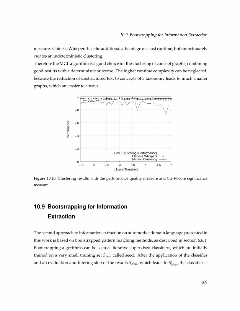
10.9 Bootstrapping for Information Extraction
measure. Chinese Whispers has the additional advantage of a fast runtime, but unfortunately
creates an indeterministic clustering.
Therefore the MCL algorithm is a good choice for the clustering of concept graphs, combining
good results with a deterministic outcome. The higher runtime complexity can be neglected,
because the reduction of unstructured text to concepts of a taxonomy leads to much smaller
graphs, which are easier to cluster.
0
0.2
0.4
0.6
0.8
1
1.5 2 2.5 3 3.5 4 4.5 5
Per
form
ance
t-Score Threshold
GMC-Clustering (Performance)Chinese WhispersMarkov Clustering
Figure 10.20: Clustering results with the performance quality measure and the t-Score significance
measure
10.9 Bootstrapping for Information
Extraction
The second approach to information extraction on automotive domain language presented in
this work is based on bootstrapped pattern matching methods, as described in section 6.6.1.
Bootstrapping algorithms can be seen as iterative supervised classifiers, which are initially
trained on a very small training set SSeed called seed. After the application of the classifier
and an evaluation and filtering step of the results SNew, which leads to S′New, the classifier is
169
10 Processing and Language Resources
trained on the merged set of SSeed and S′New. Although all kinds of supervised classifiers can
be integrated into a semi-supervised bootstrapping algorithm, the approach presented here
follows the most common approach using extraction patterns (e.g. [136]). Given an initial
seed of relation tuples, the system iteratively learns patterns P to detect those tuples, and
filters the set of tuples and patterns with respect to given confidence measures between two
succeeding iterations. Then the patterns can be used to extract new tuples, and the system
bootstraps itself.
10.9.1 Confidence Measures
To uphold quality of tuples and patterns during the bootstrapping execution and to ensure
convergence of the algorithm (see [75]), it is important to implement confidence measures
and to delete elements which do not fulfill certain thresholds.
Internal Knowledge
Literature concerned with the calculation of confidence measures for tuples or patterns
concentrates on the usage of internal knowledge, which is generated by the bootstrapping
process itself. The most popular internal confidence measure for tuples is defined in [136]. It
is based on the assumption that a tuple ti is of high quality, if it is extracted by patterns which
themselves extracted already known tuples from SSeed. Let Pi be the set of patterns which
extracted tuple ti, F(p) the number of tuples from SSeed which were extracted by p, then the
confidence is defined as:
Conf(ti) =
∑p∈Pi
log2(F(p) + 1)
|Pi|(10.19)
A confidence measure for patterns is also described in [136], and is known as the R log F
metric:
Conf(pi) =Fi
Ni· log2(Fi) (10.20)
170
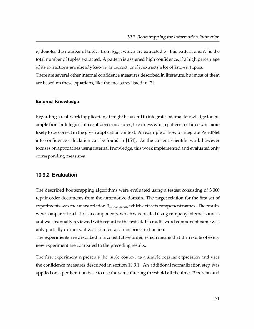
10.9 Bootstrapping for Information Extraction
Fi denotes the number of tuples from SSeed, which are extracted by this pattern and Ni is the
total number of tuples extracted. A pattern is assigned high confidence, if a high percentage
of its extractions are already known as correct, or if it extracts a lot of known tuples.
There are several other internal confidence measures described in literature, but most of them
are based on these equations, like the measures listed in [7].
External Knowledge
Regarding a real-world application, it might be useful to integrate external knowledge for ex-
ample from ontologies into confidence measures, to express which patterns or tuples are more
likely to be correct in the given application context. An example of how to integrate WordNet
into confidence calculation can be found in [154]. As the current scientific work however
focuses on approaches using internal knowledge, this work implemented and evaluated only
corresponding measures.
10.9.2 Evaluation
The described bootstrapping algorithms were evaluated using a testset consisting of 3.000
repair order documents from the automotive domain. The target relation for the first set of
experiments was the unary relation RisComponent, which extracts component names. The results
were compared to a list of car components, which was created using company internal sources
and was manually reviewed with regard to the testset. If a multi-word component name was
only partially extracted it was counted as an incorrect extraction.
The experiments are described in a constitutive order, which means that the results of every
new experiment are compared to the preceding results.
The first experiment represents the tuple context as a simple regular expression and uses
the confidence measures described in section 10.9.1. An additional normalization step was
applied on a per iteration base to use the same filtering threshold all the time. Precision and
171
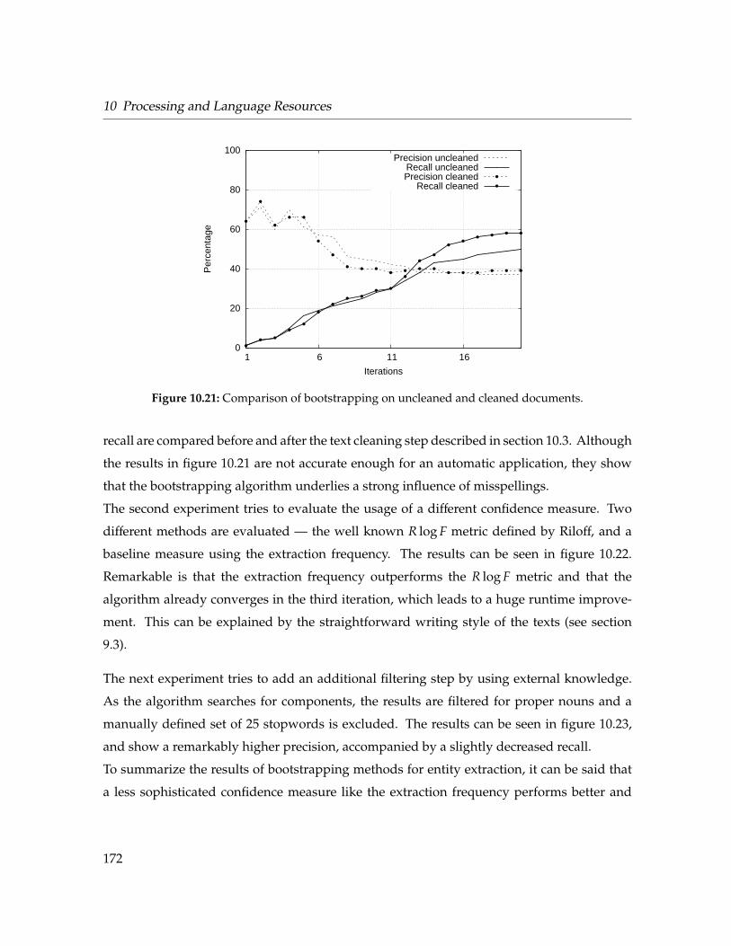
10 Processing and Language Resources
0
20
40
60
80
100
1 6 11 16
Per
cent
age
Iterations
Precision uncleanedRecall uncleanedPrecision cleaned
Recall cleaned
Figure 10.21: Comparison of bootstrapping on uncleaned and cleaned documents.
recall are compared before and after the text cleaning step described in section 10.3. Although
the results in figure 10.21 are not accurate enough for an automatic application, they show
that the bootstrapping algorithm underlies a strong influence of misspellings.
The second experiment tries to evaluate the usage of a different confidence measure. Two
different methods are evaluated — the well known R log F metric defined by Riloff, and a
baseline measure using the extraction frequency. The results can be seen in figure 10.22.
Remarkable is that the extraction frequency outperforms the R log F metric and that the
algorithm already converges in the third iteration, which leads to a huge runtime improve-
ment. This can be explained by the straightforward writing style of the texts (see section
9.3).
The next experiment tries to add an additional filtering step by using external knowledge.
As the algorithm searches for components, the results are filtered for proper nouns and a
manually defined set of 25 stopwords is excluded. The results can be seen in figure 10.23,
and show a remarkably higher precision, accompanied by a slightly decreased recall.
To summarize the results of bootstrapping methods for entity extraction, it can be said that
a less sophisticated confidence measure like the extraction frequency performs better and
172
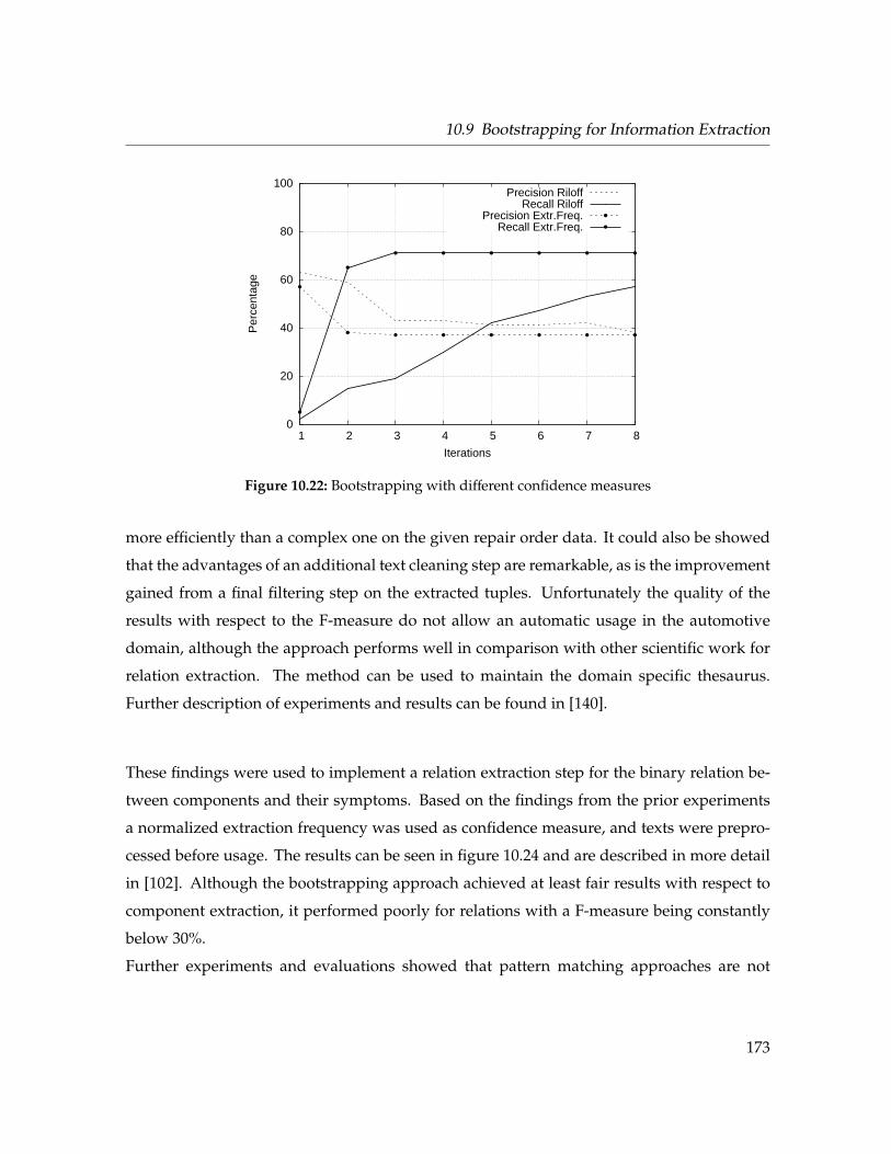
10.9 Bootstrapping for Information Extraction
0
20
40
60
80
100
1 2 3 4 5 6 7 8
Per
cent
age
Iterations
Precision RiloffRecall Riloff
Precision Extr.Freq.Recall Extr.Freq.
Figure 10.22: Bootstrapping with different confidence measures
more efficiently than a complex one on the given repair order data. It could also be showed
that the advantages of an additional text cleaning step are remarkable, as is the improvement
gained from a final filtering step on the extracted tuples. Unfortunately the quality of the
results with respect to the F-measure do not allow an automatic usage in the automotive
domain, although the approach performs well in comparison with other scientific work for
relation extraction. The method can be used to maintain the domain specific thesaurus.
Further description of experiments and results can be found in [140].
These findings were used to implement a relation extraction step for the binary relation be-
tween components and their symptoms. Based on the findings from the prior experiments
a normalized extraction frequency was used as confidence measure, and texts were prepro-
cessed before usage. The results can be seen in figure 10.24 and are described in more detail
in [102]. Although the bootstrapping approach achieved at least fair results with respect to
component extraction, it performed poorly for relations with a F-measure being constantly
below 30%.
Further experiments and evaluations showed that pattern matching approaches are not
173
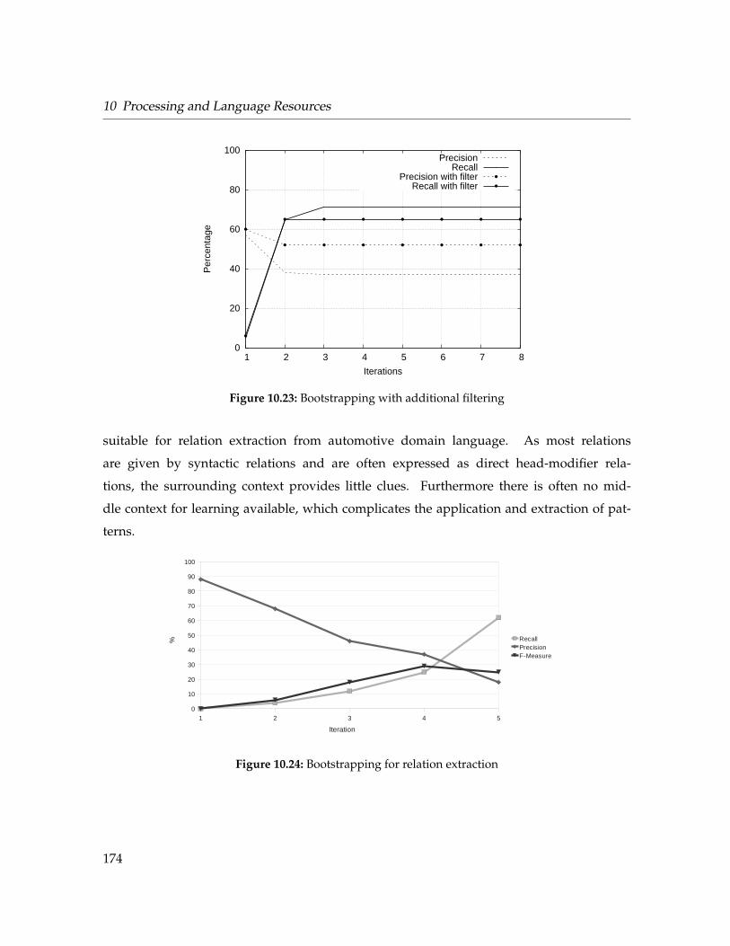
10 Processing and Language Resources
0
20
40
60
80
100
1 2 3 4 5 6 7 8
Per
cent
age
Iterations
PrecisionRecall
Precision with filterRecall with filter
Figure 10.23: Bootstrapping with additional filtering
suitable for relation extraction from automotive domain language. As most relations
are given by syntactic relations and are often expressed as direct head-modifier rela-
tions, the surrounding context provides little clues. Furthermore there is often no mid-
dle context for learning available, which complicates the application and extraction of pat-
terns.
1 2 3 4 5
0
10
20
30
40
50
60
70
80
90
100
RecallPrecisionF-Measure
Iteration
%
Figure 10.24: Bootstrapping for relation extraction
174
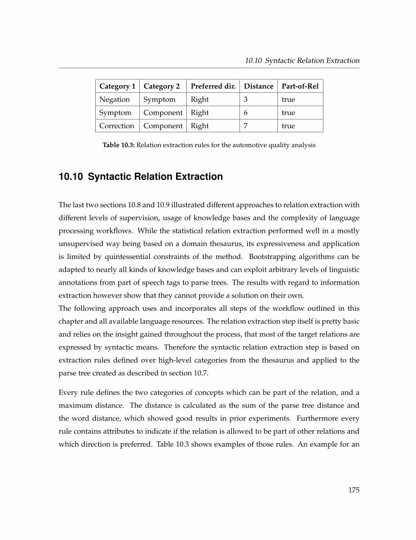
10.10 Syntactic Relation Extraction
Category 1 Category 2 Preferred dir. Distance Part-of-Rel
Negation Symptom Right 3 true
Symptom Component Right 6 true
Correction Component Right 7 true
Table 10.3: Relation extraction rules for the automotive quality analysis
10.10 Syntactic Relation Extraction
The last two sections 10.8 and 10.9 illustrated different approaches to relation extraction with
different levels of supervision, usage of knowledge bases and the complexity of language
processing workflows. While the statistical relation extraction performed well in a mostly
unsupervised way being based on a domain thesaurus, its expressiveness and application
is limited by quintessential constraints of the method. Bootstrapping algorithms can be
adapted to nearly all kinds of knowledge bases and can exploit arbitrary levels of linguistic
annotations from part of speech tags to parse trees. The results with regard to information
extraction however show that they cannot provide a solution on their own.
The following approach uses and incorporates all steps of the workflow outlined in this
chapter and all available language resources. The relation extraction step itself is pretty basic
and relies on the insight gained throughout the process, that most of the target relations are
expressed by syntactic means. Therefore the syntactic relation extraction step is based on
extraction rules defined over high-level categories from the thesaurus and applied to the
parse tree created as described in section 10.7.
Every rule defines the two categories of concepts which can be part of the relation, and a
maximum distance. The distance is calculated as the sum of the parse tree distance and
the word distance, which showed good results in prior experiments. Furthermore every
rule contains attributes to indicate if the relation is allowed to be part of other relations and
which direction is preferred. Table 10.3 shows examples of those rules. An example for an
175
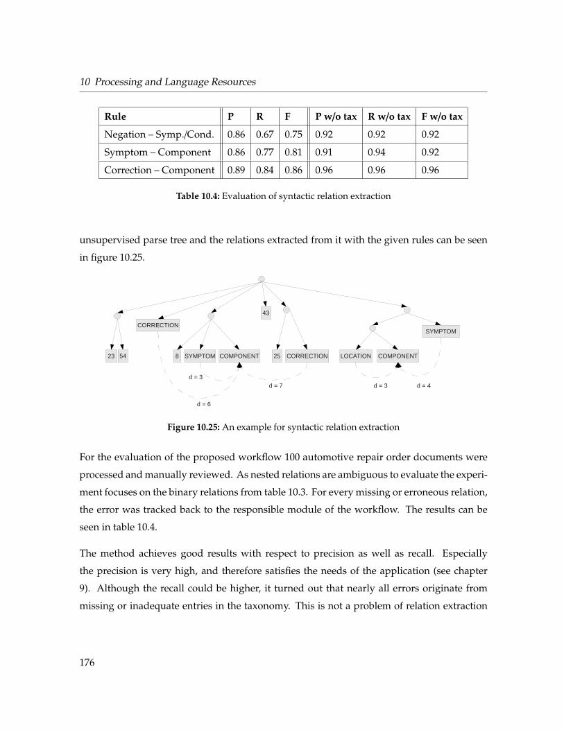
10 Processing and Language Resources
Rule P R F P w/o tax R w/o tax F w/o tax
Negation – Symp./Cond. 0.86 0.67 0.75 0.92 0.92 0.92
Symptom – Component 0.86 0.77 0.81 0.91 0.94 0.92
Correction – Component 0.89 0.84 0.86 0.96 0.96 0.96
Table 10.4: Evaluation of syntactic relation extraction
unsupervised parse tree and the relations extracted from it with the given rules can be seen
in figure 10.25.
COMPONENTLOCATIONCOMPONENT
CORRECTION
SYMPTOM CORRECTION23 54 8
43
25
SYMPTOM
d = 7 d = 3 d = 4
d = 3
d = 6
Figure 10.25: An example for syntactic relation extraction
For the evaluation of the proposed workflow 100 automotive repair order documents were
processed and manually reviewed. As nested relations are ambiguous to evaluate the experi-
ment focuses on the binary relations from table 10.3. For every missing or erroneous relation,
the error was tracked back to the responsible module of the workflow. The results can be
seen in table 10.4.
The method achieves good results with respect to precision as well as recall. Especially
the precision is very high, and therefore satisfies the needs of the application (see chapter
9). Although the recall could be higher, it turned out that nearly all errors originate from
missing or inadequate entries in the taxonomy. This is not a problem of relation extraction
176
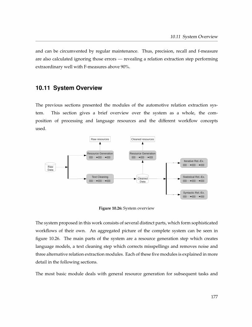
10.11 System Overview
and can be circumvented by regular maintenance. Thus, precision, recall and f-measure
are also calculated ignoring those errors — revealing a relation extraction step performing
extraordinary well with F-measures above 90%.
10.11 System Overview
The previous sections presented the modules of the automotive relation extraction sys-
tem. This section gives a brief overview over the system as a whole, the com-
position of processing and language resources and the different workflow concepts
used.
RawData
Resource Generation
Raw resources
Text CleaningCleaned
Data
Resource Generation
Cleaned resources
Iterative Rel.-Ex.
Syntactic Rel.-Ex.
Statistical Rel.-Ex.
Figure 10.26: System overview
The system proposed in this work consists of several distinct parts, which form sophisticated
workflows of their own. An aggregated picture of the complete system can be seen in
figure 10.26. The main parts of the system are a resource generation step which creates
language models, a text cleaning step which corrects misspellings and removes noise and
three alternative relation extraction modules. Each of these five modules is explained in more
detail in the following sections.
The most basic module deals with general resource generation for subsequent tasks and
177
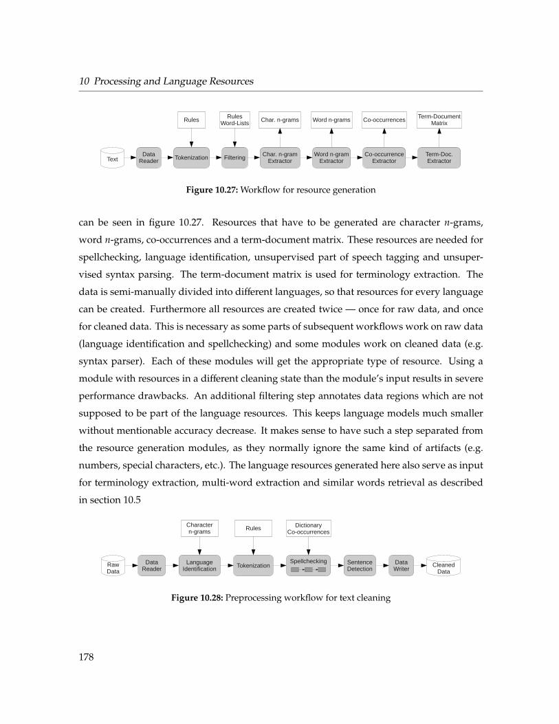
10 Processing and Language Resources
TextData
Reader FilteringTokenization
RulesRules
Word-Lists
Char. n-gramExtractor
Word n-gramExtractor
Co-occurrenceExtractor
Char. n-grams Word n-grams Co-occurrences
Term-Doc.Extractor
Term-DocumentMatrix
Figure 10.27: Workflow for resource generation
can be seen in figure 10.27. Resources that have to be generated are character n-grams,
word n-grams, co-occurrences and a term-document matrix. These resources are needed for
spellchecking, language identification, unsupervised part of speech tagging and unsuper-
vised syntax parsing. The term-document matrix is used for terminology extraction. The
data is semi-manually divided into different languages, so that resources for every language
can be created. Furthermore all resources are created twice — once for raw data, and once
for cleaned data. This is necessary as some parts of subsequent workflows work on raw data
(language identification and spellchecking) and some modules work on cleaned data (e.g.
syntax parser). Each of these modules will get the appropriate type of resource. Using a
module with resources in a different cleaning state than the module’s input results in severe
performance drawbacks. An additional filtering step annotates data regions which are not
supposed to be part of the language resources. This keeps language models much smaller
without mentionable accuracy decrease. It makes sense to have such a step separated from
the resource generation modules, as they normally ignore the same kind of artifacts (e.g.
numbers, special characters, etc.). The language resources generated here also serve as input
for terminology extraction, multi-word extraction and similar words retrieval as described
in section 10.5
RawData
DataReader
LanguageIdentification
SpellcheckingTokenization
DataWriter
CleanedData
Charactern-grams
Rules DictionaryCo-occurrences
SentenceDetection
Figure 10.28: Preprocessing workflow for text cleaning
178
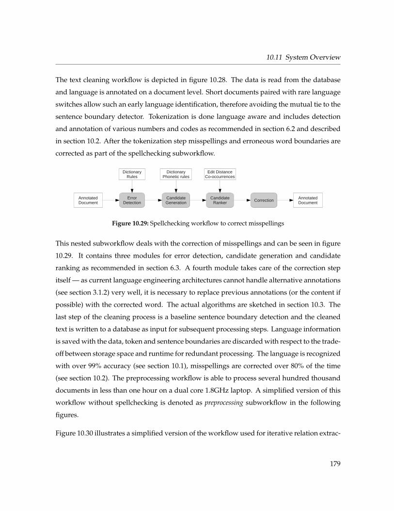
10.11 System Overview
The text cleaning workflow is depicted in figure 10.28. The data is read from the database
and language is annotated on a document level. Short documents paired with rare language
switches allow such an early language identification, therefore avoiding the mutual tie to the
sentence boundary detector. Tokenization is done language aware and includes detection
and annotation of various numbers and codes as recommended in section 6.2 and described
in section 10.2. After the tokenization step misspellings and erroneous word boundaries are
corrected as part of the spellchecking subworkflow.
CandidateGeneration
ErrorDetection
DictionaryRules
DictionaryPhonetic rules
CandidateRanker
Edit DistanceCo-occurrences
AnnotatedDocument
AnnotatedDocumentCorrection
Figure 10.29: Spellchecking workflow to correct misspellings
This nested subworkflow deals with the correction of misspellings and can be seen in figure
10.29. It contains three modules for error detection, candidate generation and candidate
ranking as recommended in section 6.3. A fourth module takes care of the correction step
itself — as current language engineering architectures cannot handle alternative annotations
(see section 3.1.2) very well, it is necessary to replace previous annotations (or the content if
possible) with the corrected word. The actual algorithms are sketched in section 10.3. The
last step of the cleaning process is a baseline sentence boundary detection and the cleaned
text is written to a database as input for subsequent processing steps. Language information
is saved with the data, token and sentence boundaries are discarded with respect to the trade-
off between storage space and runtime for redundant processing. The language is recognized
with over 99% accuracy (see section 10.1), misspellings are corrected over 80% of the time
(see section 10.2). The preprocessing workflow is able to process several hundred thousand
documents in less than one hour on a dual core 1.8GHz laptop. A simplified version of this
workflow without spellchecking is denoted as preprocessing subworkflow in the following
figures.
Figure 10.30 illustrates a simplified version of the workflow used for iterative relation extrac-
179
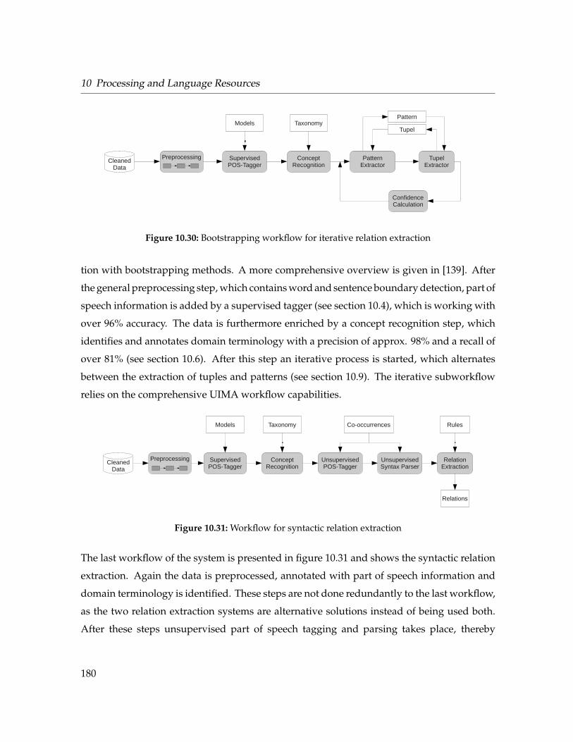
10 Processing and Language Resources
CleanedData
Preprocessing SupervisedPOS-Tagger
PatternExtractor
ConceptRecognition
TupelExtractor
Models TaxonomyPattern
ConfidenceCalculation
Tupel
Figure 10.30: Bootstrapping workflow for iterative relation extraction
tion with bootstrapping methods. A more comprehensive overview is given in [139]. After
the general preprocessing step, which contains word and sentence boundary detection, part of
speech information is added by a supervised tagger (see section 10.4), which is working with
over 96% accuracy. The data is furthermore enriched by a concept recognition step, which
identifies and annotates domain terminology with a precision of approx. 98% and a recall of
over 81% (see section 10.6). After this step an iterative process is started, which alternates
between the extraction of tuples and patterns (see section 10.9). The iterative subworkflow
relies on the comprehensive UIMA workflow capabilities.
CleanedData
Preprocessing SupervisedPOS-Tagger
ConceptRecognition
Models Taxonomy
UnsupervisedPOS-Tagger
Co-occurrences
UnsupervisedSyntax Parser
RelationExtraction
Relations
Rules
Figure 10.31: Workflow for syntactic relation extraction
The last workflow of the system is presented in figure 10.31 and shows the syntactic relation
extraction. Again the data is preprocessed, annotated with part of speech information and
domain terminology is identified. These steps are not done redundantly to the last workflow,
as the two relation extraction systems are alternative solutions instead of being used both.
After these steps unsupervised part of speech tagging and parsing takes place, thereby
180
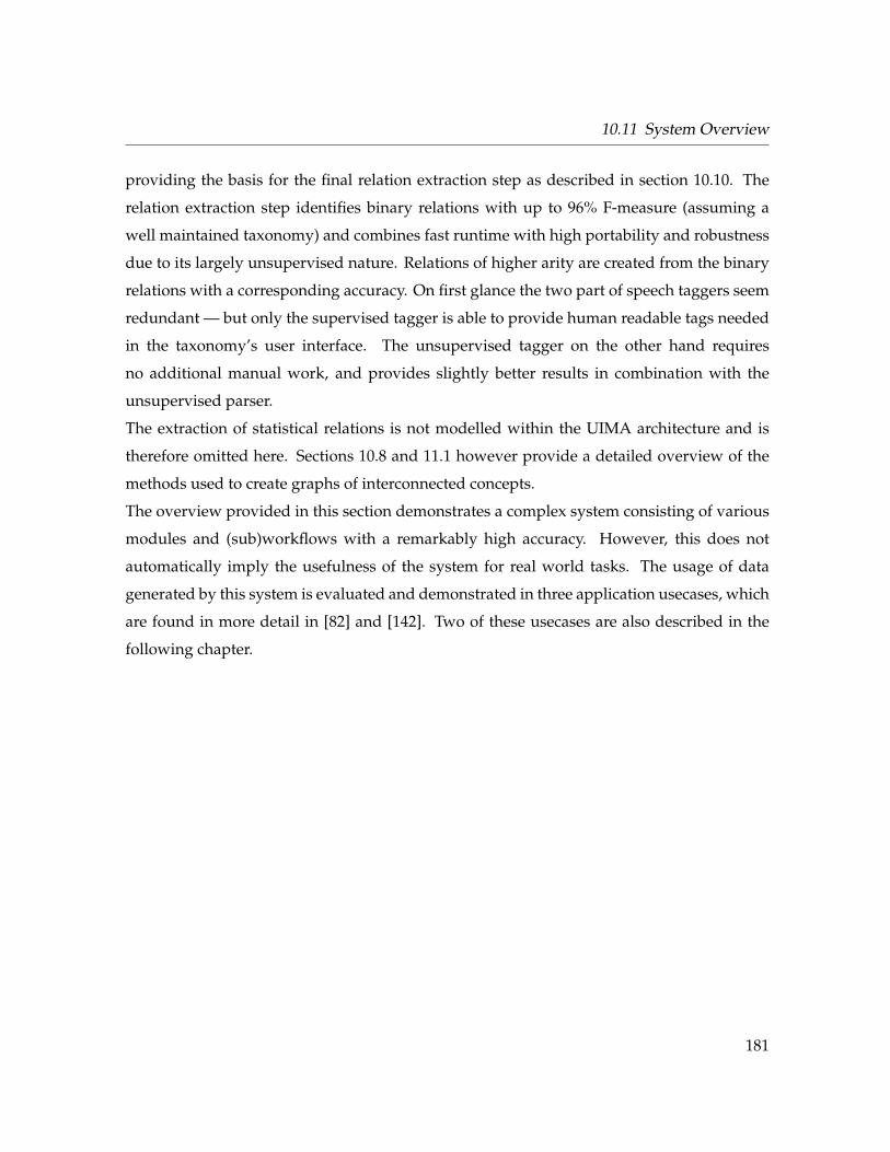
10.11 System Overview
providing the basis for the final relation extraction step as described in section 10.10. The
relation extraction step identifies binary relations with up to 96% F-measure (assuming a
well maintained taxonomy) and combines fast runtime with high portability and robustness
due to its largely unsupervised nature. Relations of higher arity are created from the binary
relations with a corresponding accuracy. On first glance the two part of speech taggers seem
redundant — but only the supervised tagger is able to provide human readable tags needed
in the taxonomy’s user interface. The unsupervised tagger on the other hand requires
no additional manual work, and provides slightly better results in combination with the
unsupervised parser.
The extraction of statistical relations is not modelled within the UIMA architecture and is
therefore omitted here. Sections 10.8 and 11.1 however provide a detailed overview of the
methods used to create graphs of interconnected concepts.
The overview provided in this section demonstrates a complex system consisting of various
modules and (sub)workflows with a remarkably high accuracy. However, this does not
automatically imply the usefulness of the system for real world tasks. The usage of data
generated by this system is evaluated and demonstrated in three application usecases, which
are found in more detail in [82] and [142]. Two of these usecases are also described in the
following chapter.
181

182
11 Application
After having analyzed the requirements from the domain, the characteristics of the
corpus and having designed, implemented and evaluated the information extraction
workflow, this chapter will present some application scenarios for the proposed work-
flow.
11.1 Root Cause Analysis
The statistical relation extraction described in section 10.8 is useful to provide a fast insight
into large amounts of texts, by creating clusters of interconnected domain terminology. This
facilitates problem detection as well as Root Cause Analysis. Given a large set of repair orders,
the different clusters represent different quality issues. By narrowing the data down on
repairs for a given damage code, a quality advocate can easily identify related problems,
error conditions and different failure types. By adding structured data like model families
and model years to the item set it is also possible to track quality problems back to the
affected product lines. For this application usecase a randomly chosen day of data (see
10.8.7), including repair order text, model name and model year was processed as described
in section 10.8. After preprocessing the texts (see sections 10.1 to 10.3), interesting concepts
were extracted and co-occurrences between them were calculated (see section 10.6). The
co-occurrence matrix is then used to cluster the items using the Chinese Whispers algorithm
with a t-Score threshold of 1.5.
183
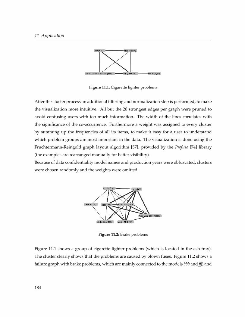
11 Application
Figure 11.1: Cigarette lighter problems
After the cluster process an additional filtering and normalization step is performed, to make
the visualization more intuitive. All but the 20 strongest edges per graph were pruned to
avoid confusing users with too much information. The width of the lines correlates with
the significance of the co-occurrence. Furthermore a weight was assigned to every cluster
by summing up the frequencies of all its items, to make it easy for a user to understand
which problem groups are most important in the data. The visualization is done using the
Fruchtermann-Reingold graph layout algorithm [57], provided by the Prefuse [74] library
(the examples are rearranged manually for better visibility).
Because of data confidentiality model names and production years were obfuscated, clusters
were chosen randomly and the weights were omitted.
Figure 11.2: Brake problems
Figure 11.1 shows a group of cigarette lighter problems (which is located in the ash tray).
The cluster clearly shows that the problems are caused by blown fuses. Figure 11.2 shows a
failure graph with brake problems, which are mainly connected to the models bbb and fff, and
184
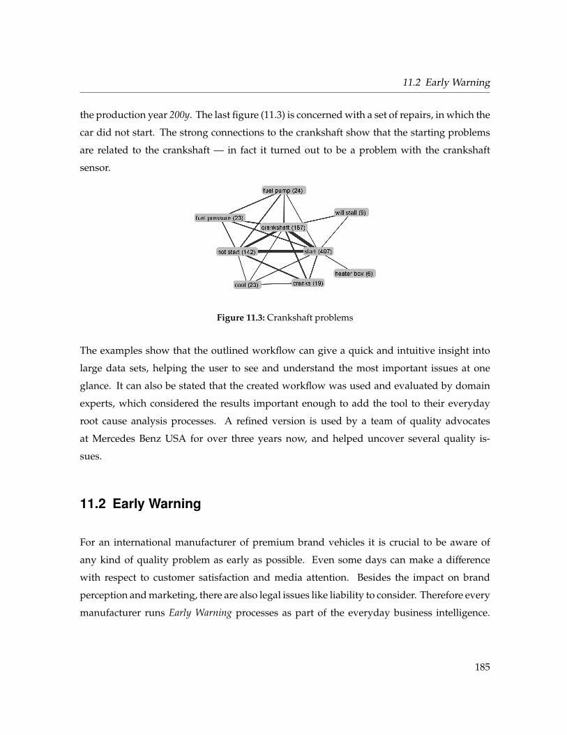
11.2 Early Warning
the production year 200y. The last figure (11.3) is concerned with a set of repairs, in which the
car did not start. The strong connections to the crankshaft show that the starting problems
are related to the crankshaft — in fact it turned out to be a problem with the crankshaft
sensor.
Figure 11.3: Crankshaft problems
The examples show that the outlined workflow can give a quick and intuitive insight into
large data sets, helping the user to see and understand the most important issues at one
glance. It can also be stated that the created workflow was used and evaluated by domain
experts, which considered the results important enough to add the tool to their everyday
root cause analysis processes. A refined version is used by a team of quality advocates
at Mercedes Benz USA for over three years now, and helped uncover several quality is-
sues.
11.2 Early Warning
For an international manufacturer of premium brand vehicles it is crucial to be aware of
any kind of quality problem as early as possible. Even some days can make a difference
with respect to customer satisfaction and media attention. Besides the impact on brand
perception and marketing, there are also legal issues like liability to consider. Therefore every
manufacturer runs Early Warning processes as part of the everyday business intelligence.
185
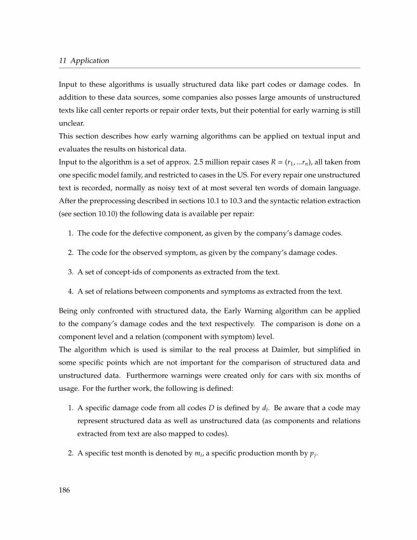
11 Application
Input to these algorithms is usually structured data like part codes or damage codes. In
addition to these data sources, some companies also posses large amounts of unstructured
texts like call center reports or repair order texts, but their potential for early warning is still
unclear.
This section describes how early warning algorithms can be applied on textual input and
evaluates the results on historical data.
Input to the algorithm is a set of approx. 2.5 million repair cases R = (r1, ...rn), all taken from
one specific model family, and restricted to cases in the US. For every repair one unstructured
text is recorded, normally as noisy text of at most several ten words of domain language.
After the preprocessing described in sections 10.1 to 10.3 and the syntactic relation extraction
(see section 10.10) the following data is available per repair:
1. The code for the defective component, as given by the company’s damage codes.
2. The code for the observed symptom, as given by the company’s damage codes.
3. A set of concept-ids of components as extracted from the text.
4. A set of relations between components and symptoms as extracted from the text.
Being only confronted with structured data, the Early Warning algorithm can be applied
to the company’s damage codes and the text respectively. The comparison is done on a
component level and a relation (component with symptom) level.
The algorithm which is used is similar to the real process at Daimler, but simplified in
some specific points which are not important for the comparison of structured data and
unstructured data. Furthermore warnings were created only for cars with six months of
usage. For the further work, the following is defined:
1. A specific damage code from all codes D is defined by dl. Be aware that a code may
represent structured data as well as unstructured data (as components and relations
extracted from text are also mapped to codes).
2. A specific test month is denoted by mi, a specific production month by p j.
186
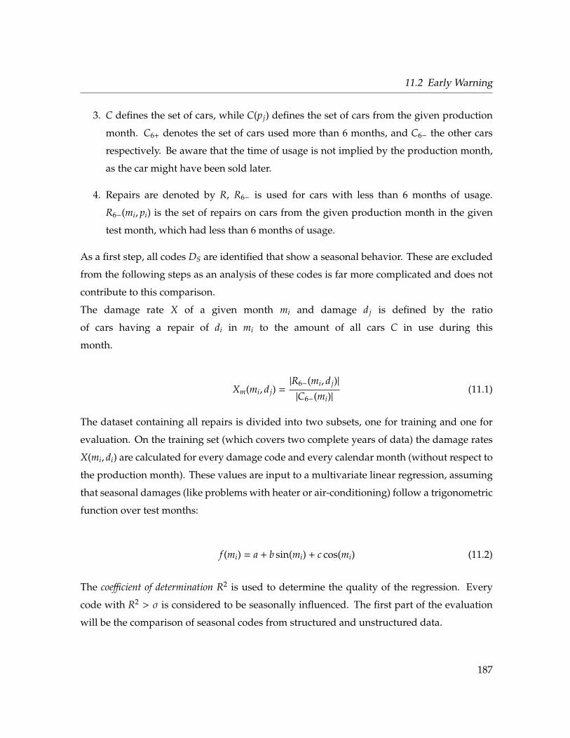
11.2 Early Warning
3. C defines the set of cars, while C(p j) defines the set of cars from the given production
month. C6+ denotes the set of cars used more than 6 months, and C6− the other cars
respectively. Be aware that the time of usage is not implied by the production month,
as the car might have been sold later.
4. Repairs are denoted by R, R6− is used for cars with less than 6 months of usage.
R6−(mi, pi) is the set of repairs on cars from the given production month in the given
test month, which had less than 6 months of usage.
As a first step, all codes DS are identified that show a seasonal behavior. These are excluded
from the following steps as an analysis of these codes is far more complicated and does not
contribute to this comparison.
The damage rate X of a given month mi and damage d j is defined by the ratio
of cars having a repair of di in mi to the amount of all cars C in use during this
month.
Xm(mi, d j) =|R6−(mi, d j)||C6−(mi)|
(11.1)
The dataset containing all repairs is divided into two subsets, one for training and one for
evaluation. On the training set (which covers two complete years of data) the damage rates
X(mi, di) are calculated for every damage code and every calendar month (without respect to
the production month). These values are input to a multivariate linear regression, assuming
that seasonal damages (like problems with heater or air-conditioning) follow a trigonometric
function over test months:
f (mi) = a + b sin(mi) + c cos(mi) (11.2)
The coefficient of determination R2 is used to determine the quality of the regression. Every
code with R2 > σ is considered to be seasonally influenced. The first part of the evaluation
will be the comparison of seasonal codes from structured and unstructured data.
187
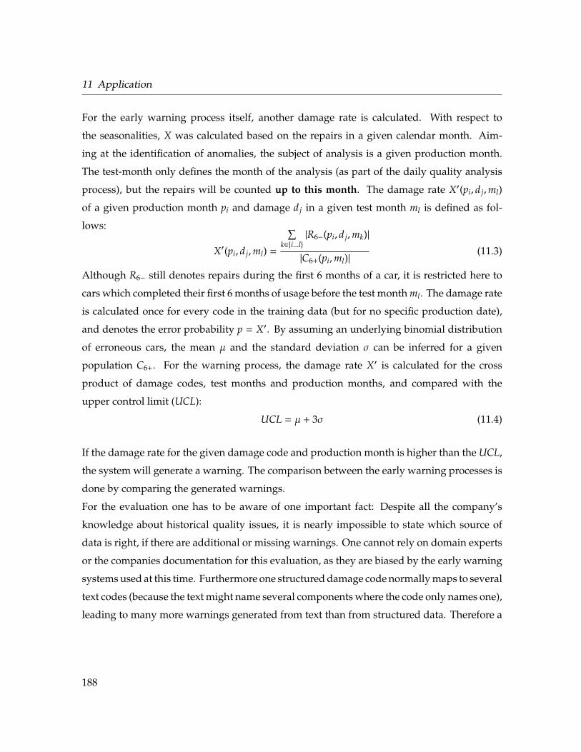
11 Application
For the early warning process itself, another damage rate is calculated. With respect to
the seasonalities, X was calculated based on the repairs in a given calendar month. Aim-
ing at the identification of anomalies, the subject of analysis is a given production month.
The test-month only defines the month of the analysis (as part of the daily quality analysis
process), but the repairs will be counted up to this month. The damage rate X′(pi, d j,ml)
of a given production month pi and damage d j in a given test month ml is defined as fol-
lows:
X′(pi, d j,ml) =
∑k∈{i...l}
|R6−(pi, d j,mk)|
|C6+(pi,ml)|(11.3)
Although R6− still denotes repairs during the first 6 months of a car, it is restricted here to
cars which completed their first 6 months of usage before the test month ml. The damage rate
is calculated once for every code in the training data (but for no specific production date),
and denotes the error probability p = X′. By assuming an underlying binomial distribution
of erroneous cars, the mean µ and the standard deviation σ can be inferred for a given
population C6+. For the warning process, the damage rate X′ is calculated for the cross
product of damage codes, test months and production months, and compared with the
upper control limit (UCL):
UCL = µ + 3σ (11.4)
If the damage rate for the given damage code and production month is higher than the UCL,
the system will generate a warning. The comparison between the early warning processes is
done by comparing the generated warnings.
For the evaluation one has to be aware of one important fact: Despite all the company’s
knowledge about historical quality issues, it is nearly impossible to state which source of
data is right, if there are additional or missing warnings. One cannot rely on domain experts
or the companies documentation for this evaluation, as they are biased by the early warning
systems used at this time. Furthermore one structured damage code normally maps to several
text codes (because the text might name several components where the code only names one),
leading to many more warnings generated from text than from structured data. Therefore a
188
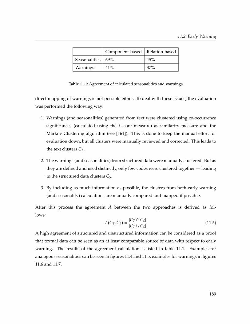
11.2 Early Warning
Component-based Relation-based
Seasonalities 69% 45%
Warnings 41% 37%
Table 11.1: Agreement of calculated seasonalities and warnings
direct mapping of warnings is not possible either. To deal with these issues, the evaluation
was performed the following way:
1. Warnings (and seasonalities) generated from text were clustered using co-occurrence
significances (calculated using the t-score measure) as similarity measure and the
Markov Clustering algorithm (see [161]). This is done to keep the manual effort for
evaluation down, but all clusters were manually reviewed and corrected. This leads to
the text clusters CT.
2. The warnings (and seasonalities) from structured data were manually clustered. But as
they are defined and used distinctly, only few codes were clustered together — leading
to the structured data clusters CS.
3. By including as much information as possible, the clusters from both early warning
(and seasonality) calculations are manually compared and mapped if possible.
After this process the agreement A between the two approaches is derived as fol-
lows:
A(CT,CS) =|CT ∩ CS|
|CT ∪ CS|(11.5)
A high agreement of structured and unstructured information can be considered as a proof
that textual data can be seen as an at least comparable source of data with respect to early
warning. The results of the agreement calculation is listed in table 11.1. Examples for
analogous seasonalities can be seen in figures 11.4 and 11.5, examples for warnings in figures
11.6 and 11.7.
189
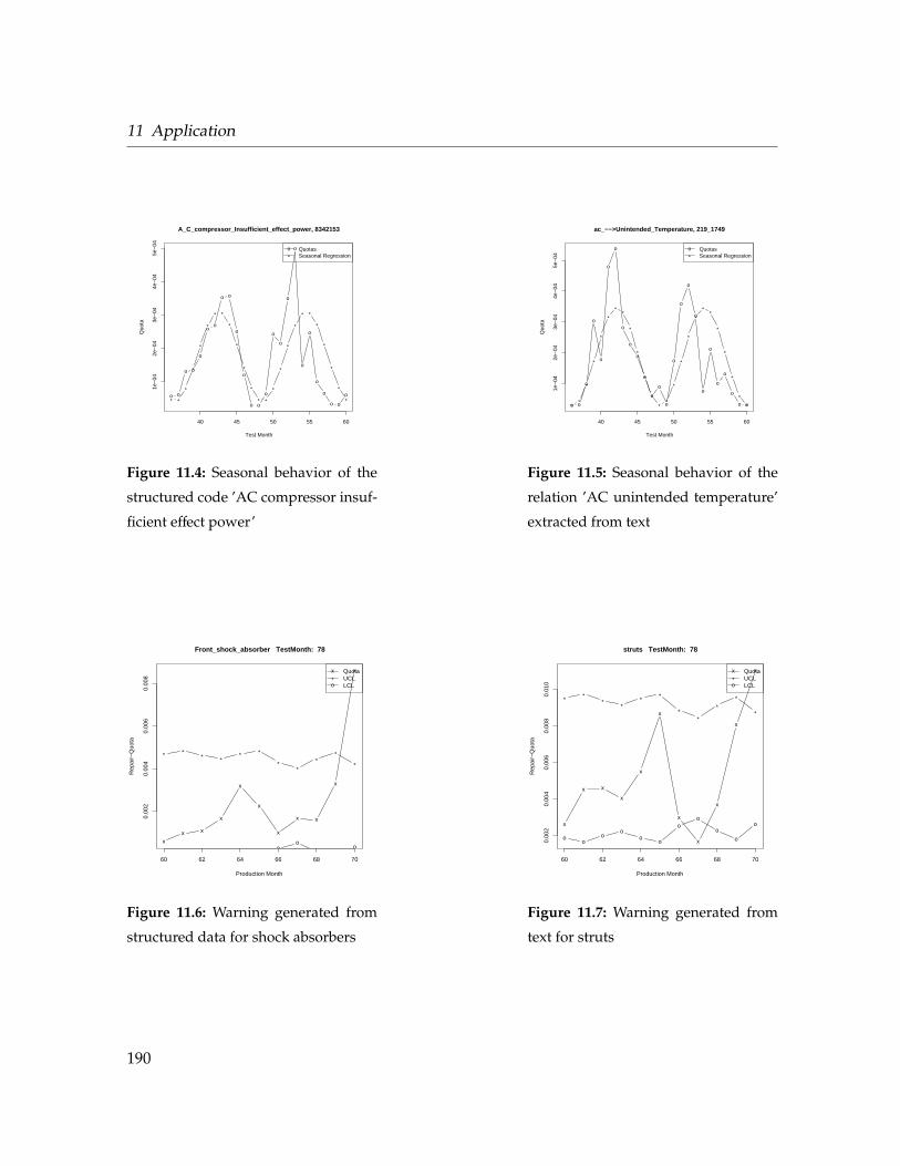
11 Application
o o
o o
o
oo
o o
o
o
o o
o
o
o
o
o
o
o
o
o
o o
o
40 45 50 55 60
1e−
042e
−04
3e−
044e
−04
5e−
04
A_C_compressor_Insufficient_effect_power, 8342153
Test Month
Quo
ta
* *
*
*
*
*
* *
*
*
*
*
* *
*
*
*
*
* *
*
*
*
*
*
o
*QuotasSeasonal Regression
Figure 11.4: Seasonal behavior of the
structured code ’AC compressor insuf-
ficient effect power’
o o
o
o
o
o
o
o
o
o
o
o
o
o
o
o
o
o
o
o
o
o
o
o o
40 45 50 55 60
1e−
042e
−04
3e−
044e
−04
5e−
04
ac_−−>Unintended_Temperature, 219_1749
Test Month
Quo
ta
**
*
*
*
*
**
*
*
*
*
**
*
*
*
*
**
*
*
*
*
*
o
*QuotasSeasonal Regression
Figure 11.5: Seasonal behavior of the
relation ’AC unintended temperature’
extracted from text
xx x
x
x
x
x
x x
x
x
60 62 64 66 68 70
0.00
20.
004
0.00
60.
008
Front_shock_absorber TestMonth: 78
Production Month
Rep
air−
Quo
ta
* ** *
* *
**
**
*
o oo o
o o
oo
oo
o
x
*o
QuotaUCLLCL
Figure 11.6: Warning generated from
structured data for shock absorbers
x
x x
x
x
x
x
x
x
x
x
60 62 64 66 68 70
0.00
20.
004
0.00
60.
008
0.01
0
struts TestMonth: 78
Production Month
Rep
air−
Quo
ta
**
**
**
**
*
*
*
oo
oo
oo
oo
o
o
o
x
*o
QuotaUCLLCL
Figure 11.7: Warning generated from
text for struts
190
11.2 Early Warning
The results show that the agreement between the generated warnings and seasonalities is
too high to be neglected. Nearly half of the calculated items could be mapped and many of
the other items were rather similar in nature, or even identical, but related to different test
months. If warnings were for example created more than six months apart from each other,
they were always considered different. Regarding the items which could be mapped, three
observations became obvious:
1. Damage codes are designed to uniquely identify a specific part of the car. They are
highly technical and very specific in nature. The concepts and relations extracted from
text are more customer centric and general. While technical codes are better suited to
find erroneous parts of the car, the text is better suited to identify the general misbehav-
ior of the car, as noted by the customer. For example several different structured codes
indicated the air conditioning as seasonally influenced, but mainly only two different
problems were derived from the text: Air conditioning which doesn’t blow cold, and
air conditioning which smells bad. Despite the many different technical parts of the
air conditioning that can possibly fail, the customer notices only two distinct problems.
Therefore it can be concluded that an early warning based on text can be important to
become aware of failures from a customer’s perspective.
2. The information from the text is suited to reinforce and verify the structured informa-
tion. Warnings which are found by both approaches can be seen as confirmed. On the
other hand, the text might help to find erroneous repairs or encoding problems. Our
evaluation identified several examples where the structured code did not fit the text.
3. For all the warnings in agreement, a closer look is taken on when the warnings were
generated. It turned out that the structured data warned earlier in five cases for
components (two cases for relations), while the text was faster in seven cases (one for
relations). In average of these cases, the structured data was two months faster (1.5 for
relations), the text was 2.1 months faster (2 for relations). Therefore it is concluded that
text warnings are important for quality analysis, as they might become evident earlier.
191
11 Application
In summary it can be said that textual early warning can be done with convincing results.
Although the warnings might not be completely identical to the ones from structured data,
they give interesting insights and reveal problems from the customers’ view. Furthermore
the traditional results can be confirmed and enriched with additional information. Regarding
these results, it is strongly suggested to include unstructured information in the automotive
early warning process.
192

Part III
Conclusion
193

12 Conclusion
This chapter summarizes the findings and results from the previous chapters, outlines the
impact of this work to real world applications, and finally concludes with an outlook to future
research.
12.1 Summary
This thesis aims to define a theory of language engineering with respect to information extrac-
tion. While other scientific work exhaustively covers the aspects of adequate infrastructures
(e.g. [44]), the process of how to define, implement and apply current state of the art methods
to a new corpus was neglected.
This work describes all elements necessary for designing a language engineering system
and how they can be interconnected to form a successful system. Part I introduces widely
used infrastructures and architectures for natural language processing systems and discusses
advantages and disadvantages with respect to different application scenarios. Especially the
availability of sophisticated workflow methods (like subworkflows and iterative workflows)
and features like analysis aware parameter and resource handling was considered crucial.
After comparing the different architectures, UIMA was found to be the most promising ap-
proach due to the advanced standardization process and the exhaustive capabilities.
Chapter 4 gives an overview over a selected subset of language statistics and describes how
they can be utilized to gain a general understanding of corpora. With respect to a given
example it is obvious that even basic characteristics like concentration or predictability provide
195
12 Conclusion
crucial insight into the data and must be considered before designing appropriate systems.
Unfortunately the formal relation between those characteristics and different language pro-
cessing methods is still unclear and cannot easily be uncovered. After introducing well
known machine learning algorithms in chapter 5, their usage in processing resources is de-
scribed in chapter 6. An important finding is the fact that processing resources need to be
carefully tailored to the domain of interest. Although nearly every method can be imple-
mented by using different machine learning algorithms, there will always be usage scenarios
demanding for a specific implementation — especially with respect to domain language.
This thesis tries to strongly emphasize its disagreement with the popular opinion of having a
’best’ method which can be employed on all kinds of textual data. The literature and findings
cited in chapter 6 document the characteristics of the different approaches with respect to
given language characteristics.
Part II shows how the conclusions of the first part help to design and implement an infor-
mation extraction system for automotive quality analysis. After characterizing the domain
(the first scientific coverage of repair order language to the writer’s knowledge) the selection,
creation and adaption of appropriate processing and language resources for the domain is
documented. It is shown how the knowledge of language characteristics can be employed to
choose methods, to avoid unnecessary work and to provide a scalable and high performance
architecture — by assuring maintainability, robustness and extendibility. Within that imple-
mentation a custom spellchecking algorithm was developed, which outperforms current state
of the art algorithms on the given domain. Furthermore a multilingual domain thesaurus
was developed, which combines the most relevant relations and considerations of WordNet
with matching capabilities for multilingual concept recognition. For the relation extraction
step a rule based approach is presented, which was specifically designed for the automotive
domain and is characterized by convincing simplicity and performance. The fact that an
approach like this might show decreased performance on other languages is just another
compelling argument in favor of carefully selecting methods with respect to the corpus.
Chapter 11 finally shows the usage of the relation extraction algorithms in a real-world appli-
cation of automotive quality analysis. Section 11.2 compares the explanatory power of textual
196

12.2 Open Questions
data with structured data and finds that the textual data provides comparable results joined
with additional insights. The results clearly show that textual data processed by information
extraction means cannot be neglected in quality processes.
In summary this thesis tries to identify all parts of information extraction systems, their inter-
relations, strengths and shortcomings and how a system can be assembled from these jigsaw
pieces. The thesis exemplifies these findings on a real world usecase, which is evaluated in
every single processing resource, and in the final application scenarios. Thereby this thesis
is the first to cover the characteristics of automotive domain language and develops innova-
tive means for context-sensitive spelling correction, multilingual domain thesauri, relation
extraction and early warning on textual data.
12.2 Open Questions
Open questions resulting from this work are especially found in the exact formal dependence
of language characteristics and language processing algorithms. Regarding the amount of
available algorithms, this connection is hard to formalize in a theoretical or even empirical
manner. The knowledge of these relations would be invaluable for future scientific work,
and could massively influence language engineering. This thesis explicitly recommends the
documentation of underlying textual characteristics in every research paper dealing with nat-
ural language processing methods. If this was done consistently, the selection of appropriate
methods for specific corpora would be much easier. Furthermore all algorithms should be
evaluated on at least two or three significantly different kinds of corpora to maximize expres-
siveness of results.
Other open questions are found with respect to the automotive usecase. Especially the ex-
tension to other languages and the infrastructural needs arising through these extensions are
interesting, and may be covered by future work. Shortcomings of the proposed system can
be found in the handling of particles, the identification of distant relations and methods to
maintain the thesaurus.
197
12 Conclusion
12.3 Application of this Work
The application scenarios presented in chapter 11 were integrated into the quality processes
of an international car manufacturer. Especially the failure graphs described in section 11.1
have now been in use for three years in the US and Germany, and are part of everyday work.
The graphs created by the proposed method give the quality advocates a quick and intuitive
insight into large textual data, and provide crucial clues about issues which might need
further attention. The method proposed for Early Warning was up to now only evaluated,
but the proposed or similar methods are very likely to be incorporated into the company’s
reporting tools in the long run.
Furthermore the preprocessing steps described in sections 10.1 to 10.3 have been in
usage for over four years now and are a solid foundation for additional reporting
steps.
198
Bibliography
[1] Tei p5: Guidelines for electronic text encoding and interchange, 11 2009. http://www.tei-
c.org/release/doc/tei-p5-doc/en/Guidelines.pdf.
[2] The apache software foundation - uima news. Website, 01 2010.
[3] Iso/tc 37/sc4 - language resources management. Website, 01 2010.
http://www.tc37sc4.org.
[4] Opennlp. Website, 01 2010. http://opennlp.sourceforge.net/index.html.
[5] Abney, S., Flickenger, S., Gdaniec, C., Grishman, C., Harrison, P., Hindle, D., Ingria,
R., Jelinek, F., Klavans, J., Liberman, M., Marcus, M., Roukos, S., Santorini, B.,
and Strzalkowski, T. Procedure for quantitatively comparing the syntactic coverage
of english grammars. In HLT ’91: Proceedings of the workshop on Speech and Natural
Language (Morristown, NJ, USA, 1991), E. Black, Ed., Association for Computational
Linguistics, pp. 306–311.
[6] Afantenos, S., Petasis, G., and Karkaletsis, V. Users Guide to Ellogon. Institute of
Informatics & Telecommunications - Software & Knowledge Engineering Laboratory,
06 2002.
[7] Agichtein, E., and Gravano, L. Snowball: Extracting relations from large plain-text
collections. In Proceedings of the Fifth ACM International Conference on Digital Libraries
(2000).
199
Bibliography
[8] Alias-i. Lingpipe 3.8.2, 01 2010. http://alias-i.com/lingpipe.
[9] Aone, C., and Ramos-Santacruz, M. Rees: A large-scale relation and event extraction
system. In ANLP (2000), pp. 76–83.
[10] Apache Software Foundation. UIMA Overview & SDK Setup, 10 2009.
[11] Apache UIMA Development Community. UIMA References (Version 2.3.0-incubating).
[12] Appelt, D. E., Bear, J., Hobbs, J. R., Israel, D., and Tyson, M. Sri international fastus
system: Muc-4 test results and analysis. In MUC4 ’92: Proceedings of the 4th conference
on Message understanding (Morristown, NJ, USA, 1992), Association for Computational
Linguistics, pp. 143–147.
[13] Appelt, D. E., Hobbs, J. R., Bear, J., Israel, D., Kameyama, M., Martin, D., Myers, K.,
and Tyson, M. Sri international fastus system: Muc-6 test results and analysis. In
MUC6 ’95: Proceedings of the 6th conference on Message understanding (Morristown, NJ,
USA, 1995), Association for Computational Linguistics, pp. 237–248.
[14] Atserias, J., Casas, B., Comelles, E., Gonzalez, M., Padro, L., and Padro, M. Freeling
1.3: Syntactic and semantic services in an open-source nlp library. In Proceedings of
the 5th International Conference on Language Resources and Evaluation (LREC’06) (2006),
pp. 48–55.
[15] Baroni, M., andBisi, S. Using cooccurrence statistics and the web to discover synonyms
in technical language. In Proceedings of LREC 2004 (2004), pp. 1725–1728.
[16] Biemann, C. Chinese whispers - an efficient graph clustering algorithm and its appli-
cation to natural language processing problems. In Proceedings of TextGraphs: the Second
Workshop on Graph Based Methods for Natural Language Processing (New York City, June
2006), Association for Computational Linguistics, pp. 73–80.
200
Bibliography
[17] Biemann, C. Unsupervised part-of-speech tagging employing efficient graph cluster-
ing. In Proceedings of the COLING/ACL-06 Student Research Workshop (Sydney, Australia,
2006).
[18] Biemann, C. Unsupervised and Knowledge-free Natural Language Processing in the Structure
Discovery Paradigm. PhD thesis, Leipzig University, 2007.
[19] Biemann, C., and Bordag, S. Lernen paradigmatischer Relationen auf iterierten Kol-
lokationen. In Anwendungen des deutschen Wortnetzes in Theorie und Praxis (2003).
[20] Biemann, C., and Teresniak, S. Disentangling from babylonian confusion - unsuper-
vised language identification. In CICLing (2005), pp. 773–784.
[21] Bilhaut, F., and Widlocher, A. Linguastream: an integrated environment for com-
putational linguistics experimentation. In EACL ’06: Proceedings of the Eleventh Con-
ference of the European Chapter of the Association for Computational Linguistics: Posters &
Demonstrations (Morristown, NJ, USA, 2006), Association for Computational Linguis-
tics, pp. 95–98.
[22] Bird, S., Day, D., Garofolo, J. S., Henderson, J., Laprun, C., and Liberman, M. Atlas:
A flexible and extensible architecture for linguistic annotation. CoRR cs.CL/0007022
(2000).
[23] Blondel, V. D. Automatic extraction of synonyms in a dictionary. In Proceedings of the
SIAM Text Mining Workshop (2002).
[24] Blumenstock, A., Schweiggert, F., and Muller, M. Rule cubes for causal investiga-
tions. In Proceedings of the 2007 Seventh IEEE International Conference on Data Mining
(Washington, DC, USA, 2007), IEEE Computer Society, pp. 53–62.
[25] Bod, R. An all-subtrees approach to unsupervised parsing. In Proceedings of the 21st
International Conference on Computational Linguistics and the 44th annual meeting of the
201
Bibliography
Association for Computational Linguistics (Stroudsburg, PA, USA, 2006), ACL-44, Associ-
ation for Computational Linguistics, pp. 865–872.
[26] Bontcheva, K., Tablan, V., Maynard, D., and Cunningham, H. Evolving GATE to
Meet New Challenges in Language Engineering. Natural Language Engineering 10, 3/4
(2004), 349—373.
[27] Borthwick, A., Sterling, J., Agichtein, E., and Grishman, R. Exploiting diverse
knowledge sources via maximum entropy in named entity recognition. In Proceedings
of the sixth workshop on very large corpora (1998), pp. 152–160.
[28] Brandes, U., Gaertler, M., and Wagner, D. Experiments on graph clustering algo-
rithms., 2003.
[29] Brants, T. Tnt - a statistical part-of-speech tagger. In Proceedings of the Sixth Applied
Natural Language Processing (ANLP-2000) (Seattle, WA, 2000).
[30] Brill, E. A simple rule-based part of speech tagger. In Proceedings of the Third Conference
on Applied Natural Language Processing (1992).
[31] Brin, S. Extracting patterns and relations from the world wide web. In WebDB Workshop
at 6th International Conference on Extending Database Technology, EDBT’98 (1998).
[32] Buechler, M. Flexible computing of co-occurrences on structured and unstructered
text. Master’s thesis, Leipzig University, 2006.
[33] Bulmer, M. G. Principles of Statistics. Dover Publications, March 1979.
[34] Callmeier, U., Eisele, A., Schafer, U., and Siegel, M. The deepthought core architec-
ture framework. In Proceedings of LREC 04 (Lisbon, Portugal, 2004).
[35] Carroll, J., Minnen, G., and Briscoe, T. Parser evaluation: Using a grammatical
relation annotation scheme, 2003.
202
Bibliography
[36] Carstensen, K.-U., Ebert, C., Jekat, S., Ebert, C., Langer, H., and Klabunde, R. Com-
puterlinguistik und Sprachtechnologie: Eine Einfuhrung. Springer, 2009. ISBN 3827420237.
[37] Cavnar, W. B., and Trenkle, J. M. N-gram-based text categorization. In Proceedings
of SDAIR-94, 3rd Annual Symposium on Document Analysis and Information Retrieval (Las
Vegas, US, 1994), pp. 161–175.
[38] Chieu, H. L., and Ng, H. T. Named entity recognition: a maximum entropy ap-
proach using global information. In Proceedings of the 19th international conference on
Computational linguistics (Morristown, NJ, USA, 2002), Association for Computational
Linguistics, pp. 1–7.
[39] Church, K. W., and Gale, W. A. Probability scoring for spelling correction. Statistics
and Computing 1, 2 (December 1991), 93–103.
[40] Collins, M., and Singer, Y. Unsupervised models for named entity classification.
In Proceedings of the Joint SIGDAT Conference on Empirical Methods in Natural Language
Processing and Very Large Corpora (1999), pp. 100–110.
[41] Copestake, A., Corbett, P., Murray-rust, P., Siddharthan, A., Teufel, S., andWaldron,
B. An architecture for language processing for scientific texts. In Proceedings of the 4th
UK E-Science All Hands Meeting (2006).
[42] Culotta, A., and Sorensen, J. Dependency tree kernels for relation extraction. In ACL
’04: Proceedings of the 42nd Annual Meeting on Association for Computational Linguistics
(Morristown, NJ, USA, 2004), Association for Computational Linguistics, pp. 423+.
[43] Cunningham, H. A definition and short history of language engineering. Nat. Lang.
Eng. 5 (March 1999), 1–16.
[44] Cunningham, H. Software Architecture for Language Engineering. PhD thesis, University
of Sheffield, 2000. http://gate.ac.uk/sale/thesis/.
203
Bibliography
[45] Cunningham, H., Maynard, D., Bontcheva, K., and Tablan, V. GATE: A framework
and graphical development environment for robust NLP tools and applications. In
Proceedings of the 40th Anniversary Meeting of the Association for Computational Linguistics
(2002).
[46] Cunningham, H., Maynard, D., and Bontcheva, K. e. a. Developing Language Processing
Components with GATE Version 5 (a User Guide). The University of Sheffield, 01 2010.
[47] Cutting, D., Kupiec, J., Pedersen, J., and Sibun, P. A practical part-of-speech tagger. In
Proceedings of the third conference on Applied natural language processing (Morristown, NJ,
USA, 1992), Association for Computational Linguistics, pp. 133–140.
[48] Damerau, F. J. A technique for computer detection and correction of spelling errors.
Commun. ACM 7, 3 (1964), 171–176.
[49] Dingare, S., Nissim, M., Finkel, J., Manning, C., and Grover, C. A system for iden-
tifying named entities in biomedical text: how results from two evaluations reflect on
both the system and the evaluations: Conference papers. Comp. Funct. Genomics 6, 1-2
(2005), 77–85.
[50] Dunning, T. Accurate methods for the statistics of surprise and coincidence. Comput.
Linguist. 19, 1 (1993), 61–74.
[51] Dunning, T. Statistical identification of language. Tech. rep., Computing Research Lab
(CRL), New Mexico State University, Las Cruces, NM, 1994.
[52] Eisner, J., and Karakos, D. Bootstrapping without the boot. In Proceedings of Hu-
man Language Technology Conference and Conference on Empirical Methods in Natural Lan-
guage Processing (Vancouver, October 2005), Association for Computational Linguistics,
pp. 395–402.
[53] Evert, S. The Statistics of Word Cooccurrences Word Pairs and Collocations. PhD thesis,
Universitat Stuttgart, August 2004.
204
Bibliography
[54] Ferrucci, D., and Lally, A. UIMA: An Architectural Approach to Unstructured Infor-
mation Processing in the Corporate Research Environment. Natural Language Engineer-
ing (2004).
[55] Fleischman, M., and Hovy, E. Fine grained classification of named entities. In Pro-
ceedings of the 19th international conference on Computational linguistics (Morristown, NJ,
USA, 2002), Association for Computational Linguistics, pp. 1–7.
[56] Foggia, P., Percannella, G., Sansone, C., andVento, M. Assessing the performance of
a graph-based clustering algorithm. In GbRPR (2007), F. Escolano and M. Vento, Eds.,
vol. 4538 of Lecture Notes in Computer Science, Springer, pp. 215–227.
[57] Fruchterman, T. M. J., and Reingold, E. M. Graph drawing by force-directed place-
ment. Softw. Pract. Exper. 21, 11 (1991), 1129–1164.
[58] Fundel, K., Kuffner, R., and Zimmer, R. Relex—relation extraction using dependency
parse trees. Bioinformatics 23 (January 2007), 365–371.
[59] Ghani, R., and Jones, R. A comparison of efficacy and assumptions of bootstrap-
ping algorithms for training information extraction systems. In Workshop on Linguistic
Knowledge Acquisition and Representation at the Third International Conference on Language
Resources and Evaluation (LREC (2002).
[60] Gimenez, J., and Marquez, L. Svmtool: A general pos tagger generator based on
support vector machines. In Proceedings of the 4th International Conference on Language
Resources and Evaluation (2004), pp. 43–46.
[61] Golding, A. R. A bayesian hybrid method for context-sensitive spelling correction,
1996.
[62] Golding, A. R., and Roth, D. A winnow-based approach to context-sensitive spelling
correction. In Machine Learning (1999), pp. 107–130.
205
Bibliography
[63] Grefenstette, G., and Tapanainen, P. What is a word, what is a sentence? Problems
of tokenization. pp. 79–87.
[64] Grishman, R. The nyu system for muc-6 or where’s the syntax? In MUC6 ’95:
Proceedings of the 6th conference on Message understanding (Morristown, NJ, USA, 1995),
Association for Computational Linguistics, pp. 167–175.
[65] Grishman, R. Tipster text phase ii architecture design. In Proceedings of a workshop on
held at Vienna, Virginia (Morristown, NJ, USA, 1996), Association for Computational
Linguistics, pp. 249–305.
[66] Grishman, R., and Sterling, J. New York University: description of the Proteus
system as used for MUC-5. In MUC5 ’93: Proceedings of the 5th conference on Message
understanding (Morristown, NJ, USA, 1993), Association for Computational Linguistics,
pp. 181–194.
[67] Grishman, R., and Sundheim, B. Design of the muc-6 evaluation. In MUC6 ’95:
Proceedings of the 6th conference on Message understanding (Morristown, NJ, USA, 1995),
Association for Computational Linguistics, pp. 1–11.
[68] Grover, C., Matheson, C., Mikheev, A., andMoens, M. LT TTT — a flexible tokenisa-
tion tool. In Proc. LREC 2000 (2000).
[69] Gunning, R. The Technique of Clear Writing. McGraw-Hill, New York, 1952.
[70] Gunter Neumann, B. S. Experiments on robust nl question interpretation and multi-
layered document annotation for a cross-language question/answering system. In
proceedings of the CLEF 2004 working notes (9 2004).
[71] Hammarstrom, H. A fine-grained model for language identification, 2007.
[72] Hanisch, D., Fundel, K., Mevissen, H. T., Zimmer, R., and Fluck, J. Prominer: rule-
based protein and gene entity recognition. BMC Bioinformatics 6 Suppl 1 (2005).
206
Bibliography
[73] Hearst, M. A. Automatic acquisition of hyponyms from large text corpora. Tech. Rep.
S2K-92-09, University of California, Berkeley, 1992.
[74] Heer, J., Card, S. K., and Landay, J. A. Prefuse: a toolkit for interactive information
visualization. In CHI ’05: Proceedings of the SIGCHI conference on Human factors in
computing systems (New York, NY, USA, 2005), ACM, pp. 421–430.
[75] Heyer, G., Quasthoff, U., andWittig, T. Text Mining: Wissensrohstoff Text : Konzepte,
Algorithmen, Ergebnisse. W3L-Verl., Herdecke [u.a.], 2006.
[76] Holmes, D. Authorship attribution. Computers and the Humanities 28 (1994), 87–106.
10.1007/BF01830689.
[77] hui Chiang, T., shin Chang, J., yu Lin, M., and yih Su, K. Statistical models for word
segmentation and unknown resolution. In Proceedings of ROCLING-92 (1992), pp. 121–
146.
[78] Hanig, C. Improvements in Unsupervised Co-Occurrence Based Parsing. In Proceed-
ings of the Fourteenth Conference on Computational Natural Language Learning (Uppsala,
Sweden, 2010), no. July, Association for Computational Linguistics, pp. 1–8.
[79] Hanig, C. Improvements in unsupervised co-occurrence based parsing. In Proceedings
of the Fourteenth Conference on Computational Natural Language Learning (Stroudsburg,
PA, USA, 2010), CoNLL ’10, Association for Computational Linguistics, pp. 1–8.
[80] Hanig, C., Bordag, S., and Quasthoff, U. Unsuparse: Unsupervised parsing with
unsupervised part of speech tagging. In Proceedings of the Sixth International Language
Resources and Evaluation (LREC’08) (Marrakech, Morocco, 2008).
[81] Hanig, C., and Schierle, M. Relation extraction based on unsupervised syntactic
parsing. Text Mining Services (2009), 65–70.
207
Bibliography
[82] Hanig, C., Schierle, M., and Trabold, D. Comparison of structured vs. unstructured
data for industrial quality analysis. In Proceedings of The World Congress on Engineering
and Computer Science (2010), pp. pp432–438.
[83] Ide, N. Corpus encoding standard: SGML guidelines for encoding linguistic corpora. In
Proceedings of the First International Language Resources and Evaluation Conference (1998),
pp. 463–70.
[84] Ide, N., Bonhomme, P., and Romary, L. XCES: An XML-based encoding standard
for linguistic corpora. In Proceedings of the Second International Language Resources and
Evaluation Conference. Paris: European Language Resources Association (2000).
[85] Ide, N., Romary, L., de la Clergerie, E., and Dialogue, E. L. E. International standard
for a linguistic annotation framework. Journal of Natural Language Engineering 10 (2003).
[86] Imai, M. Kaizen: The Key to Japan’s Competitive Success. McGraw-Hill, New York, NY,
1986.
[87] Iria, J. T-rex: A flexible relation extraction framework. In In Proceedings of the 8th Annual
Colloquium for the UK Special Interest Group for Computational Linguistics (CLUK’05 (2005).
[88] Islam, A., and Inkpen, D. Real-word spelling correction using google web it 3-grams. In
EMNLP ’09: Proceedings of the 2009 Conference on Empirical Methods in Natural Language
Processing (Morristown, NJ, USA, 2009), Association for Computational Linguistics,
pp. 1241–1249.
[89] Isozaki, H., and Kazawa, H. Efficient support vector classifiers for named entity
recognition. In Proceedings of the 19th international conference on Computational linguistics
(Morristown, NJ, USA, 2002), Association for Computational Linguistics, pp. 1–7.
[90] Jackson, P., and Moulinier, I. Natural language processing for online applications. Text
retrieval, extraction and categorization, vol. 5 of Natural Language Processing. Benjamins,
Amsterdam, Philadelphia, 2002.
208
Bibliography
[91] Jiang, J., and Zhai, C. A systematic exploration of the feature space for relation
extraction. In Human Language Technologies 2007: The Conference of the North American
Chapter of the Association for Computational Linguistics; Proceedings of the Main Conference
(Rochester, New York, April 2007), Association for Computational Linguistics, pp. 113–
120.
[92] Karttunen, L., Chanod, J.-P., Grefenstette, G., and Schille, A. Regular expressions
for language engineering. Nat. Lang. Eng. 2, 4 (1996), 305–328.
[93] Kazama, J., Makino, T., Ohta, Y., and Tsujii, J. Tuning support vector machines for
biomedical named entity recognition. In Proceedings of the ACL-02 Workshop on Natural
Language Processing in the Biomedical Domain (2002), pp. 1–8.
[94] Kernighan, M. D., Church, K. W., and Gale, W. A. A spelling correction program
based on a noisy channel model. In Association for Computational Linguistics (1990),
pp. 205–210.
[95] Kirshenbaum, E., Suermondt, J., Forman, G., and Forman, G. Pragmatic text mining:
minimizing human effort to quantify many issues in call logs. In In Proc. of the 12 th
ACM SIGKDD International Conference on Knowledge Discovery and Data Mining (KDD
(2006), ACM Press, pp. 852–861.
[96] Klein, D. The Unsupervised Learning of Natural Language Structure. PhD thesis, Stanford
University, 2005.
[97] Knuth, D. E. Fundamental Algorithms, vol. 1 of The Art of Computer Programming.
Addison-Wesley, Reading, Massachusetts, 10 Jan. 1973.
[98] Krauthammer, M., and Nenadic, G. Term identification in the biomedical literature.
J. of Biomedical Informatics 37, 6 (2004), 512–526.
209
Bibliography
[99] Krieger, H.-U. SDL - A description language for building NLP systems. In Proceedings
of the HLTNAACL Workshop on the Software Engineering and Architecture of Language
Technology Systems, SEALTS (2003), pp. 84–91.
[100] Kruengkrai, C., Srichaivattana, P., Sornlertlamvanich, V., and Isahara, H. Lan-
guage identification based on string kernels. In Proceedings of the 5th International
Symposium on Communications and Information Technologies (ISCIT-2005 (2005), pp. 896–
899.
[101] Kukich, K. Techniques for automatically correcting words in text. ACM Comput. Surv.
24, 4 (1992), 377–439.
[102] Kappeler, R. Relationenextraktion und Text-Klassifikation in domanen-spezifischen
Textkorpora. Master’s thesis, Ulm University, 2007.
[103] Lally, A., Verspoor, K., andNyberg, E. Unstructured information management archi-
tecture (uima) version 1.0, March 2009.
[104] Lehmann, M. Implementierung eines Text-Mining-Systems auf Basis des UIMA-
Frameworks. Master’s thesis, Universitat Leipzig, 2006.
[105] Liu, H. Montylingua: An end-to-end natural language processor with common sense.
[106] Lodhi, H., Shawe-Taylor, J., Cristianini, N., andWatkins, C. J. C. H. Text classification
using string kernels. In NIPS (2000), pp. 563–569.
[107] Loper, E., and Bird, S. Nltk: The natural language toolkit. In Proceedings of the ACL
Workshop on Effective Tools and Methodologies for Teaching Natural Language Processing and
Computational Linguistics. Philadelphia: Association for Computational Linguistics (2002).
[108] M., B., and Hanig, C. Using the internet as sensor for customer perception. In Pro-
ceedings of the Fachtagung zum Text- und Data Mining fur die Qualitatsanalyse in der
Automobilindustrie (2011), pp. 49–55.
210
Bibliography
[109] Magerman, D. M. Statistical decision-tree models for parsing. In Proceedings of the 33rd
Annual Meeting of the Association for Computational Linguistics (1995), pp. 276–283.
[110] Mahn, M. Evaluation und Verknupfung von Kookkurrenzen hoherer Ordnung und
Probabilistic Latent Semantic Analysis. Master’s thesis, Leipzig University, 2005.
[111] Mangu, L., andBrill, E. Automatic rule acquisition for spelling correction. In ICML ’97:
Proceedings of the Fourteenth International Conference on Machine Learning (San Francisco,
CA, USA, 1997), Morgan Kaufmann Publishers Inc., pp. 187–194.
[112] Manning, C., and Schutze, H. Foundations of Statistical Natural Language Processing.
MIT Press, Cambridge, MA, 1999.
[113] Marcus, M. P., Marcinkiewicz, M. A., and Santorini, B. Building a large annotated
corpus of english: the penn treebank. Comput. Linguist. 19 (June 1993), 313–330.
[114] Martins, B., and Silva, M. J. Language identification in web pages. In SAC ’05:
Proceedings of the 2005 ACM symposium on Applied computing (New York, NY, USA,
2005), ACM, pp. 764–768.
[115] Matsuo, Y. Clustering Using Small World Structure. In Knowledge-Based Intelligent
Information and Engineering Systems (2002).
[116] McCallum, A., and Li, W. Early results for named entity recognition with conditional
random fields, feature induction and web-enhanced lexicons. In Proceedings of the
seventh conference on Natural language learning at HLT-NAACL 2003 (Morristown, NJ,
USA, 2003), Association for Computational Linguistics, pp. 188–191.
[117] Mccarthy, J. F., and Lehnert, W. G. Using decision trees for coreference resolution. In
Proceedings of the Fourteenth International Joint Conference on Artificial Intelligence (1995),
pp. 1050–1055.
[118] McKelvie, D., Brew, C., and Thompson, H. S. Using SGML as a Basis for Data-Intensive
Natural Language Processing. In Computers and the Humanities (1998), pp. 367–388.
211
Bibliography
[119] Mikheev, A., Moens, M., andGrover, C. Named entity recognition without gazetteers.
In Proceedings of the Ninth Conference of the European Chapter of the Association for Compu-
tational Linguistics (1999), pp. 1–8.
[120] Miller, G. A., Beckwith, R., Fellbaum, C., Gross, D., andMiller, K. J. Introduction to
WordNet: An on-line lexical database. Int J Lexicography 3, 4 (January 1990), 235–244.
[121] Mitchell, T. M. Machine Learning. McGraw-Hill, New York, 1997.
[122] Mitkov, R. Language Engineering on the Highway: New Perspectives for the Multi-
lingual Society. In Proceedings of NLPRS (1995).
[123] Muller, M., Schlieder, C., and Blumenstock, A. Application of bayesian partition
models in warranty data analysis. In SDM (2009), pp. 121–132.
[124] Nadeau, D., and Sekine, S. A survey of named entity recognition and classification.
Linguisticae Investigationes 30, 1 (January 2007), 3–26. Publisher: John Benjamins Pub-
lishing Company.
[125] Nadeau, D., Turney, P. D., and Matwin, S. Unsupervised named-entity recognition:
Generating gazetteers and resolving ambiguity. In Canadian Conference on AI (2006),
L. Lamontagne and M. Marchand, Eds., vol. 4013 of Lecture Notes in Computer Science,
Springer, pp. 266–277.
[126] Paliouras, G., Karkaletsis, V., Petasis, G., and Spyropoulo, C. D. Learning decision
trees for named-entity recognition and classification. In Proceedings of the 14th European
Conference on Artificial Intelligence (ECAI 2000) (August 2000).
[127] Palmer, D. D. A trainable rule-based algorithm for word segmentation. In ACL-35:
Proceedings of the 35th Annual Meeting of the Association for Computational Linguistics and
Eighth Conference of the European Chapter of the Association for Computational Linguistics
(Morristown, NJ, USA, 1997), Association for Computational Linguistics, pp. 321–328.
212
Bibliography
[128] Petasis, G., Karkaletsis, V., Paliouras, G., Androutsopoulos, I., and Spyropoulos,
C. D. Ellogon: A new text engineering platform. In Proceedings of the Third International
Conference on Language Resources and Evaluation (LREC 2002), Las Palmas, Canary Islands
(2002), pp. 72–78.
[129] Philips, L. Hanging on the metaphone. Computer Language Magazine 7, 12 (Dec. 1990),
38ff.
[130] Ponte, J. Use: A retargetable word segmentation procedure for information retrieval.
Tech. rep., Amherst, MA, USA, 1996.
[131] Press, W. H., Teukolsky, S. A., Vetterling, W. T., and Flannery, B. P. Numerical Recipes
3rd Edition: The Art of Scientific Computing, 3 ed. Cambridge University Press, September
2007.
[132] Pyzdek, T., andKeller, P. The Six Sigma Handbook. McGraw-Hill Professional; 3 edition,
2009.
[133] Quinlan, J. R. Induction of decision trees. Machine Learning 1, 1 (1986), 81–106.
[134] Riloff, E. Automatically constructing a dictionary for information extraction tasks. In
National Conference on Artificial Intelligence (1993), pp. 811–816.
[135] Riloff, E. Automatically generating extraction patterns from untagged text. In
AAAI/IAAI, Vol. 2 (1996), pp. 1044–1049.
[136] Riloff, E., and Thelen, M. A bootstrapping method for learning semantic lexicons
using extraction pattern contexts. In Proceedings of the 2002 Conference on Empirical
Methods in Natural Language processing (2002).
[137] Ruch, P., Baud, R., and Geissbuhler, A. Toward filling the gap between interactive
and fully-automatic spelling correction using the linguistic context. In Proceedings of
the IEEE Workshop on Natural Language Processing and Knowledge Engineering (NLPKE)
(2001).
213
Bibliography
[138] Schafer, U. Middleware for creating and combining multi-dimensional nlp markup.
In NLPXML ’06: Proceedings of the 5th Workshop on NLP and XML (Morristown, NJ, USA,
2006), Association for Computational Linguistics, pp. 81–84.
[139] Schierle, M. Extraktion von Entitaten und Relationen mit Bootstrapping-Verfahren.
Master’s thesis, Ulm University, 2006.
[140] Schierle, M., and Schulz, S. Bootstrapping algorithms for an application in the auto-
motive domain. In Proceedings of the Sixth International Conference on Machine Learning
and Applications (Washington, DC, USA, 2007), ICMLA ’07, IEEE Computer Society,
pp. 198–203.
[141] Schierle, M., Schulz, S., and Ackermann, M. From spelling correction to text clean-
ing – using context information. In Data Analysis, Machine Learning and Applications
Proceedings of the 31st Annual Conference of the Gesellschaft fur Klassifikation e.V., Albert-
Ludwigs-University Freiburg, March 7–9, 2007 (2007).
[142] Schierle, M., andTrabold, D. Extraction of failure graphs from structured and unstruc-
tured data. In Proceedings of the 2008 Seventh International Conference on Machine Learning
and Applications (Washington, DC, USA, 2008), IEEE Computer Society, pp. 324–330.
[143] Schmid, H. Part-of-speech tagging with neural networks. In Proceedings of the 15th
conference on Computational linguistics (Morristown, NJ, USA, 1994), Association for
Computational Linguistics, pp. 172–176.
[144] Schmid, H. Probabilistic part-of-speech tagging using decision trees. In International
Conference on New Methods in Language Processing (Manchester, UK, 1994).
[145] Schnitzler, S., and Eitrich, T. Eine Einfuhrung zu String-Kernen fur die Sequenz-
analyse mit Support-Vektor-Maschinen und anderen Kern-basierten Lernalgorithmen.
Tech. rep., Forschungszentrum Julich GmbH, Zentralinstitut fur Angewandte Mathe-
matik, 2006.
214
Bibliography
[146] Schwenker, F. Data Mining Methoden - Skript zur Vorlesung, 10 2003. Universitat
Ulm.
[147] Schafer, U. Shallow, deep and hybrid processing with uima and heart of gold. In
Proceedings of the LREC-2008 Workshop Towards Enhanced Interoperability for Large HLT
Systems: UIMA for NLP, 6th International Conference on Language Resources and Evaluation.
LREC-2008, May 26 - June 1, Marrakesh, Morocco (2008), ELRA, pp. 43–50.
[148] Schafer, U., Uszkoreit, H., Federmann, C., Marek, T., and Zhang, Y. Extracting
and querying relations in scientific papers. In KI 2008: Advances in Artificial Intelligence
(2008), A. Dengel, K. Berns, T. Breuel, F. Bomarius, and T. Roth-Berghofer, Eds., vol. 5243
of Lecture Notes in Computer Science, Springer Berlin / Heidelberg, pp. 127–134.
[149] Schutze, H. Word space. In Advances in Neural Information Processing Systems 5 (1993),
Morgan Kaufmann, pp. 895–902.
[150] Schutze, H. Distributional part-of-speech tagging. In Proceedings of 7th Conference of the
European Chapter of the Association for Computational Linguistics (1995).
[151] Schutze, H. Automatic word sense discrimination. Journal of Computational Linguistics
24 (1998), 97–123.
[152] Seginer, Y. Fast unsupervised incremental parsing. In Proceedings of the 45th Annual
Meeting of the Association of Computational Linguistics (Prague, Czech Republic, 2007),
vol. 45, Association for Computational Linguistics, pp. 384—-391.
[153] Sibun, P., and Reynar, J. Language identification: Examining the issues. pp. 125–135.
[154] Stevenson, M. An unsupervised wordnet-based algorithm for relation extraction. In
LREC04 Workshop on ”Beyond Named Entity Recognition: Semantic labelling for NLP tasks”
(2004).
215
Bibliography
[155] Stevenson, M., and Greenwood, M. A semantic approach to IE pattern induction.
In Proceedings of the 43rd Annual Meeting of the Association for Computational Linguistics
(ACL’05) (Ann Arbor, Michigan, June 2005), Association for Computational Linguistics,
pp. 379–386.
[156] Tesitelova, M. Quantitive Linguistics. John Benjamins Publishing Company, Amster-
dam/Philadelphia, 1992.
[157] Tesniere, L. Elements de syntaxe structurale. C. Klincksieck, 1959.
[158] Toutanova, K., Klein, D., Manning, C. D., and Singer, Y. Feature-rich part-of-speech
tagging with a cyclic dependency network. In NAACL ’03: Proceedings of the 2003
Conference of the North American Chapter of the Association for Computational Linguistics
on Human Language Technology (Morristown, NJ, USA, 2003), Association for Compu-
tational Linguistics, pp. 173–180.
[159] Toutanova, K., andManning, C. D. Enriching the knowledge sources used in a maxi-
mum entropy part-of-speech tagger. In Proceedings of the 2000 Joint SIGDAT conference
on Empirical methods in natural language processing and very large corpora (Morristown,
NJ, USA, 2000), Association for Computational Linguistics, pp. 63–70.
[160] Trabold, D. Konzeption und Realisierung eines multilingualen Systems zur Erken-
nung benannter Entitaten. Master’s thesis, Leipzig University, 2007.
[161] van Dongen, S. M. Graph clustering by flow simulation. PhD thesis, 2000.
[162] Vossen, P., and Letteren, C. C. Eurowordnet: a multilingual database for information
retrieval. In Proceedings of the DELOS workshop on Cross-language Information Retrieval
(1997), pp. 5–7.
[163] Wagner, R. A., and Fischer, M. J. The string-to-string correction problem. J. ACM 21,
1 (1974), 168–173.
216
Bibliography
[164] Wang, T., Li, Y., Bontcheva, K., Cunningham, H., andWang, J. Automatic extraction
of hierarchical relations from text. In Proceedings of the Third European Semantic Web
Conference (ESWC 2006), Budva (2006).
[165] Watts, D. J., and Strogatz, S. H. Collective dynamics of ’small-world’ networks. Nature
393, 6684 (June 1998), 440–442.
[166] Wetzel, D. Semiuberwachtes Lernen einer lexikalischen Wissensbasis fur ein
Informations-Extraktionssystems. Master’s thesis, Ulm University, 2009.
[167] White, T. Can’t beat jazzy. Internet, 20.05.2006, 09 2004. Online available at http:
//www-128.ibm.com/developerworks/java/library/j-jazzy/.
[168] Wilcox-O’Hearn, L. A., Hirst, G., and Budanitsky, A. Real-word spelling correction
with trigrams: A reconsideration of the mays, damerau, and mercer model. In CICLing
(2008), pp. 605–616.
[169] Witten, I. H., and Frank, E. Data Mining : Praktische Werkzeuge und Techniken fur das
maschinelle Lernen. Hanser, Munchen [u.a.], 2001.
[170] Wittenburg P., Broeder D., S. B. Meta-description for language resources - a proposal
for a meta description standard for language resources, 05 2000.
[171] Yangarber, R. Counter-training in discovery of semantic patterns. In ACL ’03: Proceed-
ings of the 41st Annual Meeting on Association for Computational Linguistics (Morristown,
NJ, USA, 2003), Association for Computational Linguistics, pp. 343–350.
[172] Yangarber, R., Grishman, R., Tapanainen, P., andHuttunen, S. Automatic acquisition
of domain knowledge for information extraction. In Proceedings of the 18th International
Conference on Computational Linguistics (2000).
[173] Zelenko, D., Aone, C., and Richardella, A. Kernel methods for relation extraction.
71–78.
217
Bibliography
[174] Zhang, H. The Optimality of Naive Bayes. In FLAIRS Conference (2004), V. Barr and
Z. Markov, Eds., AAAI Press.
[175] Zhou, G., and Su, J. Named entity recognition using an hmm-based chunk tagger.
In ACL ’02: Proceedings of the 40th Annual Meeting on Association for Computational
Linguistics (Morristown, NJ, USA, 2002), Association for Computational Linguistics,
pp. 473–480.
[176] Zipf, G. Human behaviour and the principle of least-effort. Addison-Wesley, Cam-
bridge, MA, 1949.
[177] Zobel, J., and Dart, P. Finding approximate matches in large lexicons. Softw. Pract.
Exper. 25, 3 (1995), 331–345.
218