Embed Size (px)
Citation preview

Lake Shore Model 475 Gaussmeter User’s Manual
Lake Shore Cryotronics, Inc. 575 McCorkle Blvd. Westerville, Ohio 43082-8888 USA
E-mail Addresses: [email protected] [email protected]
Visit Our Website At: www.lakeshore.com
Fax: (614) 891-1392 Telephone: (614) 891-2243
Methods and apparatus disclosed and described herein have been developed solely on company funds of Lake Shore Cryotronics, Inc. No government or other contractual support or relationship whatsoever has existed which in any way affects or mitigates proprietary rights of Lake Shore Cryotronics, Inc. in these developments. Methods and apparatus disclosed herein may be subject to U.S. Patents existing or applied for. Lake Shore Cryotronics, Inc. reserves the right to add, improve, modify, or withdraw functions, design modifications, or products at any time without notice. Lake Shore shall not be liable for errors contained herein or for incidental or consequential damages in connection with furnishing, performance, or use of this material. Revision: 2.3 P/N 119-036 25 July 2017
User’s Manual
Model 475 DSP Gaussmeter
Lake Shore Model 475 Gaussmeter User’s Manual
LIMITED WARRANTY STATEMENT WARRANTY PERIOD: THREE (3) YEARS
1. Lake Shore warrants that products manufactured by Lake Shore (the "Product") will be free from defects in materials and workmanship for three years from the date of Purchaser's physical receipt of the Product (the "Warranty Period"). If Lake Shore receives notice of any such defects during the Warranty Period and the defective Product is shipped freight prepaid back to Lake Shore, Lake Shore will, at its option, either repair or replace the Product (if it is so defective) without charge for parts, service labor or associated customary return shipping cost to the Purchaser. Replacement for the Product may be by either new or equivalent in performance to new. Replacement or repaired parts, or a replaced Product, will be warranted for only the unexpired portion of the original warranty or 90 days (whichever is greater).
2. Lake Shore warrants the Product only if the Product has been sold by an authorized Lake Shore employee, sales
representative, dealer or an authorized Lake Shore original equipment manufacturer (OEM).
3. The Product may contain remanufactured parts equivalent to new in performance or may have been subject to incidental use when it is originally sold to the Purchaser.
4. The Warranty Period begins on the date the Product ships from Lake Shore’s plant.
5. This limited warranty does not apply to defects in the Product resulting from (a) improper or inadequate
installation (unless OT&V services are performed by Lake Shore), maintenance, repair or calibration, (b) fuses, software, power surges, lightning and non-rechargeable batteries, (c) software, interfacing, parts or other supplies not furnished by Lake Shore, (d) unauthorized modification or misuse, (e) operation outside of the published specifications, (f) improper site preparation or site maintenance (g) natural disasters such as flood, fire, wind, or earthquake, or (h) damage during shipment other than original shipment to you if shipped through a Lake Shore carrier.
6. This limited warranty does not cover: (a) regularly scheduled or ordinary and expected recalibrations of the
Product; (b) accessories to the Product (such as probe tips and cables, holders, wire, grease, varnish, feed throughs, etc.); (c) consumables used in conjunction with the Product (such as probe tips and cables, probe holders, sample tails, rods and holders, ceramic putty for mounting samples, Hall sample cards, Hall sample enclosures, etc.); or, (d) non-Lake Shore branded Products that are integrated with the Product.
7. To the extent allowed by applicable law,, this limited warranty is the only warranty applicable to the Product and replaces all other warranties or conditions, express or implied, including, but not limited to, the implied warranties or conditions of merchantability and fitness for a particular purpose. Specifically, except as provided herein. Lake Shore undertakes no responsibility that the products will be fit for any particular purpose for which you may be buying the Products. Any implied warranty is limited in duration to the warranty period. No oral or written information, or advice given by the Company, its Agents or Employees, shall create a warranty or in any way increase the scope of this limited warranty. Some countries, states or provinces do not allow limitations on an implied warranty, so the above limitation or exclusion might not apply to you. This warranty gives you specific legal rights and you might also have other rights that vary from country to country, state to state or province to province.
8. Further, with regard to the United Nations Convention for International Sale of Goods (CISC,) if CISG is found
to apply in relation to this agreement, which is specifically disclaimed by Lake Shore, then this limited warranty excludes warranties that: (a) the Product is fit for the purpose for which goods of the same description would ordinarily be used, (b) the Product is fit for any particular purpose expressly or impliedly made known to Lake Shore at the time of the conclusion of the contract, (c) the Product is contained or packaged in a manner usual for such goods or in a manner adequate to preserve and protect such goods where it is shipped by someone other than a carrier hired by Lake Shore.
Lake Shore Model 475 Gaussmeter User’s Manual
9. Lake Shore disclaims any warranties of technological value or of non-infringement with respect to the Product and Lake Shore shall have no duty to defend, indemnify, or hold harmless you from and against any or all damages or costs incurred by you arising from the infringement of patents or trademarks or violation or copyrights by the Product.
10. THIS WARRANTY IS NOT TRANSFERRABLE. This warranty is not transferrable.
11. Except to the extent prohibited by applicable law, neither Lake Shore nor any of its subsidiaries, affiliates or
suppliers will be held liable for direct, special, incidental, consequential or other damages (including lost profit, lost data, or downtime costs) arising out of the use, inability to use or result of use of the product, whether based in warranty, contract, tort or other legal theory, regardless whether or not Lake Shore has been advised of the possibility of such damages. Purchaser's use of the Product is entirely at Purchaser's risk. Some countries, states and provinces do not allow the exclusion of liability for incidental or consequential damages, so the above limitation may not apply to you.
12. This limited warranty gives you specific legal rights, and you may also have other rights that vary within or
between jurisdictions where the product is purchased and/or used. Some jurisdictions do not allow limitation in certain warranties, and so the above limitations or exclusions of some warranties stated above may not apply to you.
13. Except to the extent allowed by applicable law, the terms of this limited warranty statement do not exclude,
restrict or modify the mandatory statutory rights applicable to the sale of the product to you.
CERTIFICATION Lake Shore certifies that this product has been inspected and tested in accordance with its published specifications and that this product met its published specifications at the time of shipment. The accuracy and calibration of this product at the time of shipment are traceable to the United States National Institute of Standards and Technology (NIST); formerly known as the National Bureau of Standards (NBS).
FIRMWARE LIMITATIONS Lake Shore has worked to ensure that the Model 475 firmware is as free of errors as possible, and that the results you obtain from the instrument are accurate and reliable. However, as with any computer-based software, the possibility of errors exists. In any important research, as when using any laboratory equipment, results should be carefully examined and rechecked before final conclusions are drawn. Neither Lake Shore nor anyone else involved in the creation or production of this firmware can pay for loss of time, inconvenience, loss of use of the product, or property damage caused by this product or its failure to work, or any other incidental or consequential damages. Use of our product implies that you understand the Lake Shore license agreement and statement of limited warranty.
FIRMWARE LICENSE AGREEMENT The firmware in this instrument is protected by United States copyright law and international treaty provisions. To maintain the warranty, the code contained in the firmware must not be modified. Any changes made to the code is at the user’s risk. Lake Shore will assume no responsibility for damage or errors incurred as result of any changes made to the firmware. Under the terms of this agreement you may only use the Model 475 firmware as physically installed in the instrument. Archival copies are strictly forbidden. You may not decompile, disassemble, or reverse engineer the firmware. If you suspect there are problems with the firmware, return the instrument to Lake Shore for repair under the terms of the Limited Warranty specified above. Any unauthorized duplication or use of the Model 475 firmware in whole or in part, in print, or in any other storage and retrieval system is forbidden.

Lake Shore Model 475 Gaussmeter User’s Manual
TRADEMARK ACKNOWLEDGMENT Many manufacturers and sellers claim designations used to distinguish their products as trademarks. Where those designations appear in this manual and Lake Shore was aware of a trademark claim, they appear with initial capital letters and the ™ or ® symbol.
MS-DOS® and Windows/95/98/NT/2000® are trademarks of Microsoft Corp. NI-488.2™ is a trademark of National Instruments. PC, XT, AT, and PS-2 are trademarks of IBM.
Electromagnetic Compatibility (EMC) for the Model 475 Gaussmeter Electromagnetic Compatibility (EMC) of electronic equipment is a growing concern worldwide. Emissions of and immunity to electromagnetic interference is now part of the design and manufacture of most electronics. To qualify for the CE Mark, the Model 475 meets or exceeds the requirements of the European EMC Directive 89/336/EEC as a CLASS A product. A Class A product is allowed to radiate more RF than a Class B product and must include the following warning:
WARNING: This is a Class A product. In a domestic environment, this product may cause radio interference in which case the user may be required to take adequate measures. The instrument was tested under normal operating conditions with a probe and interface cables attached. If the installation and operating instructions in the User’s Manual are followed, there should be no degradation in EMC performance. This instrument is not intended for use in close proximity to RF Transmitters such as two-way radios and cell phones. Exposure to RF interference greater than that found in a typical laboratory environment may disturb the sensitive measurement circuitry of the instrument. Pay special attention to instrument cabling. Improperly installed cabling may defeat even the best EMC protection. For the best performance from any precision instrument, follow the installation instructions in the User’s Manual. In addition, the installer of the Model 475 should consider the following: • Shield measurement and computer interface cables. • Leave no unused or unterminated cables attached to the instrument. • Make cable runs as short and direct as possible. Higher radiated emissions is possible with long cables. • Do not tightly bundle cables that carry different types of signals.
Lake Shore Model 475 Gaussmeter User’s Manual
EU DECLARATION OF CONFORMITY
This declaration of conformity is issued under the sole responsibility of the manufacturer. Manufacturer: Lake Shore Cryotronics, Inc. 575 McCorkle Boulevard Westerville, OH 43082 USA Object of the declaration: Model(s): 475 Description: Gaussmeter The object of the declaration described above is in conformity with the relevant Union harmonization legislation: 2014/35/EU Low Voltage Directive 2014/30/EU EMC Directive 2011/65/EU RoHS Directive References to the relevant harmonized standards used to the specification in relation to which conformity is declared: EN 61010-1:2010
Overvoltage Category II Pollution Degree 2
EN 61326-1:2013 Class A Controlled Electromagnetic Environment
EN 50581:2012
Signed for and on behalf of: Place, Date: Westerville, OH USA Scott Ayer 21-JUL-2017 Director of Quality & Compliance

Lake Shore Model 475 Gaussmeter User’s Manual
Copyright © 2003 – 2017 by Lake Shore Cryotronics, Inc. All rights reserved. No portion of this manual may be reproduced, stored in a retrieval system, or transmitted, in any form or by any means, electronic, mechanical, photocopying, recording, or otherwise, without the express written permission of Lake Shore.
Lake Shore Model 475 Gaussmeter User’s Manual
Table of Contents i
TABLE OF CONTENTS
Chapter/Section Title Page 1 INTRODUCTION ....................................................................................................................... 1-1 1.0 GENERAL .............................................................................................................................. 1-1 1.1 DESCRIPTION ....................................................................................................................... 1-1 1.1.1 Advanced Features ............................................................................................................. 1-2 1.1.2 Measurement Features ....................................................................................................... 1-3 1.1.3 Probe Support ..................................................................................................................... 1-3 1.1.4 Display and Interface Features ........................................................................................... 1-4 1.2 SPECIFICATIONS ................................................................................................................. 1-5 1.3 SAFETY SUMMARY .............................................................................................................. 1-5 1.4 SAFETY SYMBOLS ............................................................................................................... 1-6 2 BACKGROUND ........................................................................................................................ 2-1 2.0 GENERAL .............................................................................................................................. 2-1 2.1 MODEL 475 THEORY OF OPERATION ............................................................................... 2-1 2.1.1 Sampled Data Systems ...................................................................................................... 2-1 2.1.2 Digital Signal Processing .................................................................................................... 2-1 2.1.3 Limitations of Sampled Data Systems ................................................................................ 2-1 2.1.4 Model 475 System Overview .............................................................................................. 2-2 2.1.5 DC Measurement ................................................................................................................ 2-3 2.1.6 RMS Measurement ............................................................................................................. 2-3 2.1.7 Peak Measurement ............................................................................................................. 2-4 2.2 FLUX DENSITY OVERVIEW ................................................................................................. 2-5 2.2.1 What is Flux Density? ......................................................................................................... 2-5 2.2.2 How Flux Density (B) Differs from Magnetic Field Strength (H) ......................................... 2-5 2.3 HALL MEASUREMENT ......................................................................................................... 2-5 2.3.1 Active Area .......................................................................................................................... 2-6 2.3.2 Polarity ................................................................................................................................ 2-6 2.3.3 Orientation .......................................................................................................................... 2-7 2.4 FIELD CONTROL .................................................................................................................. 2-7 2.4.1 Closed Loop PI Control ....................................................................................................... 2-7 2.4.1.1 Proportional (P) ............................................................................................................... 2-8 2.4.1.2 Integral (I) ........................................................................................................................ 2-8 2.4.1.3 Manual Output ................................................................................................................. 2-8 2.4.2 Tuning a Closed Loop PI Controller ................................................................................. 2-10 2.4.2.1 Tuning Proportional ....................................................................................................... 2-10 2.4.2.2 Tuning Integral ............................................................................................................... 2-10 3 INSTALLATION ........................................................................................................................ 3-1 3.0 GENERAL .............................................................................................................................. 3-1 3.1 INSPECTION AND UNPACKING .......................................................................................... 3-1 3.2 REAR PANEL DEFINITION ................................................................................................... 3-2 3.3 LINE INPUT ASSEMBLY ....................................................................................................... 3-3 3.3.1 Line Voltage ........................................................................................................................ 3-3 3.3.2 Line Fuse and Fuse Holder ................................................................................................ 3-3 3.3.3 Power Cord ......................................................................................................................... 3-3 3.3.4 Power Switch ...................................................................................................................... 3-3 3.4 PROBE INPUT CONNECTION ............................................................................................. 3-4 3.5 PROBE HANDLING AND OPERATION ................................................................................ 3-4 3.5.1 Probe Handling ................................................................................................................... 3-4 3.5.2 Probe Operation ................................................................................................................. 3-5 3.5.3 Probe Accuracy Considerations ......................................................................................... 3-6 3.6 AUXILIARY I/O CONNECTION ............................................................................................. 3-7 3.7 RACK MOUNTING ................................................................................................................. 3-8
Lake Shore Model 475 Gaussmeter User’s Manual
ii Table of Contents
TABLE OF CONTENTS
Chapter/Paragraph Title Page 4 OPERATION .............................................................................................................................. 4-1 4.0 GENERAL ............................................................................................................................... 4-1 4.1 TURNING POWER ON .......................................................................................................... 4-1 4.2 DISPLAY DEFINITION ........................................................................................................... 4-2 4.2.1 Display Units ....................................................................................................................... 4-2 4.2.2 Display and LED Annunciators ........................................................................................... 4-2 4.3 KEYPAD DEFINITION ............................................................................................................ 4-3 4.3.1 Key Descriptions ................................................................................................................. 4-3 4.3.2 General Keypad Operation.................................................................................................. 4-4 4.4 DISPLAY SETUP ................................................................................................................... 4-4 4.4.1 Two-Line Display Configuration .......................................................................................... 4-4 4.4.2 Display Brightness ............................................................................................................... 4-5 4.5 UNITS ..................................................................................................................................... 4-5 4.6 DC MEASUREMENT MODE .................................................................................................. 4-6 4.6.1 DC Operation Select Range and Autorange ....................................................................... 4-6 4.6.2 DC Operation Resolution and Filtering ............................................................................... 4-7 4.6.3 DC Operation Zero Probe ................................................................................................... 4-7 4.6.4 DC Operation Max Hold ...................................................................................................... 4-8 4.6.4.1 Magnitude or Algebraic .................................................................................................... 4-8 4.6.4.2 Max/Min Display Setting ................................................................................................ 4-10 4.6.5 DC Operation Reset .......................................................................................................... 4-10 4.6.6 DC Operation Relative ...................................................................................................... 4-10 4.6.7 DC Operation Analog Output 1 and 2 ............................................................................... 4-11 4.7 RMS MEASUREMENT MODE ............................................................................................. 4-12 4.7.1 RMS Operation Select Range and Autorange .................................................................. 4-12 4.7.2 RMS Operation Filter Selection ......................................................................................... 4-13 4.7.2.1 Wide Band Filters ........................................................................................................... 4-14 4.7.2.2 Narrow Band Filters ....................................................................................................... 4-15 4.7.2.3 Lowpass Filters .............................................................................................................. 4-15 4.7.3 RMS Operation Frequency Measurement ........................................................................ 4-17 4.7.4 RMS Operation Reading Rate .......................................................................................... 4-17 4.7.5 RMS Operation Max Hold ................................................................................................. 4-18 4.7.5.1 Max/Min Display Setting ................................................................................................ 4-18 4.7.6 RMS Operation Reset ....................................................................................................... 4-18 4.7.7 RMS Operation Relative.................................................................................................... 4-18 4.7.8 RMS Operation Analog Output 1 and 2 ............................................................................ 4-19 4.8 PEAK MEASUREMENT MODE ........................................................................................... 4-20 4.8.1 Peak Operation Select Range ........................................................................................... 4-20 4.8.2 Peak Operation Periodic/Pulse Setup ............................................................................... 4-21 4.8.3 Peak Operation Display Setting ........................................................................................ 4-21 4.8.4 Peak Operation Reset ....................................................................................................... 4-21 4.8.5 Peak Operation Frequency Measurement ........................................................................ 4-21 4.8.6 Peak Operation Relative ................................................................................................... 4-22 4.8.7 Peak Operation Analog Output 1 and 2 ............................................................................ 4-22 4.9 TEMPERATURE MEASUREMENT ..................................................................................... 4-23 4.10 ALARM ................................................................................................................................. 4-23 4.11 RELAYS ................................................................................................................................ 4-26 4.12 ANALOG OUTPUT 3 ............................................................................................................ 4-27 4.12.1 Analog Output 3 Mode Setting .......................................................................................... 4-27 4.12.2 Analog Output 3 Polarity ................................................................................................... 4-29 4.12.3 Analog Output 3 Volt limit .................................................................................................. 4-29 4.13 LOCKING THE KEYPAD ...................................................................................................... 4-30 4.14 DEFAULT PARAMETER VALUES....................................................................................... 4-30
Lake Shore Model 475 Gaussmeter User’s Manual
Table of Contents iii
TABLE OF CONTENTS
Chapter/Paragraph Title Page 5 ADVANCED OPERATION........................................................................................................ 5-1 5.0 GENERAL .............................................................................................................................. 5-1 5.1 PROBE MANAGEMENT ........................................................................................................ 5-1 5.1.1 Clear Probe Zero Calibration .............................................................................................. 5-1 5.1.2 Probe Serial Number .......................................................................................................... 5-1 5.1.3 Field and Temperature Compensation ............................................................................... 5-1 5.1.4 Extension Cable .................................................................................................................. 5-2 5.2 HALL GENERATOR .............................................................................................................. 5-3 5.2.1 User Programmable Cable ................................................................................................. 5-3 5.2.2 Ohms Measurement Mode ................................................................................................. 5-5 5.3 FIELD CONTROL .................................................................................................................. 5-5 5.3.1 Control On/Off setting ......................................................................................................... 5-5 5.3.2 Changing Control Setpoint .................................................................................................. 5-5 5.3.3 P and I settings ................................................................................................................... 5-6 5.3.4 Control Setpoint Ramp Rate ............................................................................................... 5-6 5.3.5 Control Slope Limit ............................................................................................................. 5-7 5.3.6 Field Control Versus Reading Resolution ........................................................................... 5-7 5.4 DATALOG .............................................................................................................................. 5-7 5.5 TRIGGERING ........................................................................................................................ 5-8 6 COMPUTER INTERFACE OPERATION .................................................................................. 6-1 6.0 GENERAL .............................................................................................................................. 6-1 6.1 IEEE-488 INTERFACE .......................................................................................................... 6-1 6.1.1 Changing IEEE-488 Interface Parameters ......................................................................... 6-2 6.1.2 Remote/Local Operation ..................................................................................................... 6-2 6.1.3 IEEE-488 Command Structure ........................................................................................... 6-2 6.1.3.1 Bus Control Commands .................................................................................................. 6-2 6.1.3.2 Common Commands ....................................................................................................... 6-3 6.1.3.3 Device Specific Commands............................................................................................. 6-3 6.1.3.4 Message Strings .............................................................................................................. 6-3 6.1.3.5 Highspeed Binary Output Configuration .......................................................................... 6-4 6.1.4 Status System ..................................................................................................................... 6-5 6.1.4.1 Overview .......................................................................................................................... 6-5 6.1.4.2 Status Register Sets ........................................................................................................ 6-8 6.1.4.3 Status Byte and Service Request (SRQ) ........................................................................ 6-9 6.1.5 IEEE Interface Example Programs ................................................................................... 6-12 6.1.5.1 IEEE-488 Interface Board Installation for Visual Basic Program .................................. 6-12 6.1.5.2 Visual Basic IEEE-488 Interface Program Setup .......................................................... 6-14 6.1.5.3 Program Operation ........................................................................................................ 6-17 6.1.6 Troubleshooting ................................................................................................................ 6-17 6.2 SERIAL INTERFACE OVERVIEW ...................................................................................... 6-18 6.2.1 Changing Baud Rate ........................................................................................................ 6-18 6.2.2 Physical Connection ......................................................................................................... 6-18 6.2.3 Hardware Support ............................................................................................................. 6-19 6.2.4 Character Format .............................................................................................................. 6-19 6.2.5 Message Strings ............................................................................................................... 6-19 6.2.6 Message Flow Control ...................................................................................................... 6-20 6.2.7 Serial Interface Example Programs .................................................................................. 6-20 6.2.7.1 Visual Basic Serial Interface Program Setup ................................................................ 6-21 6.2.7.2 Program Operation ........................................................................................................ 6-24 6.2.8 Troubleshooting ................................................................................................................ 6-24 6.3 COMMAND SUMMARY ....................................................................................................... 6-25 6.3.1 Interface Commands (Alphabetical Listing) ...................................................................... 6-27
Lake Shore Model 475 Gaussmeter User’s Manual
iv Table of Contents
TABLE OF CONTENTS
Chapter/Paragraph Title Page 7 PROBES AND ACCESSORIES ................................................................................................ 7-1 7.0 GENERAL ............................................................................................................................... 7-1 7.1 MODELS ................................................................................................................................. 7-1 7.2 ACCESSORIES ...................................................................................................................... 7-1 7.3 LAKE SHORE STANDARD PROBES .................................................................................... 7-2 7.3.1 Hall Probe Selection Criteria ............................................................................................... 7-2 7.3.2 Radiation Effects on Gaussmeter Probes ........................................................................... 7-4 7.3.3 Probe Accuracy Considerations .......................................................................................... 7-4 7.3.4 Probe Specifications ............................................................................................................ 7-5 7.4 PROBE ACCESSORIES ........................................................................................................ 7-5 7.5 HALL GENERATOR ............................................................................................................... 7-7 7.5.1 Hall Generator Handling ...................................................................................................... 7-7 7.5.2 Hall Generator Lead Wires .................................................................................................. 7-7 7.5.3 Using a Hall Generator with the Model 475 ........................................................................ 7-7 7.5.4 Attachment to A User Programmable Cable ....................................................................... 7-8 7.5.5 Hall Generator Specifications .............................................................................................. 7-8 7.6 HELMHOLTZ COIL LOW FIELD STANDARDS ..................................................................... 7-9 7.7 REFERENCE MAGNETS ..................................................................................................... 7-11 7.8 ZERO GAUSS CHAMBER ................................................................................................... 7-12 8 SERVICE ................................................................................................................................... 8-1 8.0 GENERAL ............................................................................................................................... 8-1 8.1 CONTACTING LAKE SHORE CRYOTRONICS .................................................................... 8-1 8.2 RETURNING PRODUCTS TO LAKE SHORE ....................................................................... 8-1 8.3 FUSE DRAWER ..................................................................................................................... 8-2 8.4 LINE VOLTAGE SELECTION ................................................................................................ 8-2 8.5 FUSE REPLACEMENT .......................................................................................................... 8-2 8.6 ERROR MESSAGES ............................................................................................................. 8-3 8.7 ELECTROSTATIC DISCHARGE ........................................................................................... 8-4 8.7.1 Identification of Electrostatic Discharge Sensitive Components ......................................... 8-4 8.7.2 Handling Electrostatic Discharge Sensitive Components ................................................... 8-4 8.8 ENCLOSURE TOP REMOVAL AND REPLACEMENT ......................................................... 8-5 8.9 FIRMWARE REPLACEMENT ................................................................................................ 8-5 8.10 CONNECTOR AND CABLE DEFINITIONS ........................................................................... 8-7 8.10.1 Serial Interface Cable Wiring............................................................................................... 8-9 8.10.2 IEEE-488 INTERFACE Connector .................................................................................... 8-10 8.11 CALIBRATION PROCEDURE.............................................................................................. 8-11 8.11.1 Equipment Required for Calibration .................................................................................. 8-11 8.11.2 Gauusmeter Calibration .................................................................................................... 8-11 8.11.2.1 Gaussmeter Calibration, 100 mA Excitation Ranges ..................................................... 8-11 8.11.2.2 Gaussmeter Calibration, 10 mA Excitation Ranges ....................................................... 8-12 8.11.2.3 Gaussmeter Calibration, 1 mA Excitation Ranges ......................................................... 8-13 8.11.3 Temperature Measurement Calibration ............................................................................ 8-14 8.11.4 Analog Output 2 and 3 Calibration .................................................................................... 8-14 8.11.4.1 Analog Output 2 Calibration ........................................................................................... 8-14 8.11.4.2 Analog Output 3 Calibration ........................................................................................... 8-15 8.11.5 Calibration Specific Interface Commands ......................................................................... 8-16 A UNITS FOR MAGNETIC PROPERTIES .................................................................................. A-1
Lake Shore Model 475 Gaussmeter User’s Manual
Introduction 1-1
CHAPTER 1
INTRODUCTION 1.0 GENERAL This chapter provides an introduction to the Model 475 DSP Gaussmeter. The Model 475 was designed and manufactured in the United States of America by Lake Shore Cryotronics, Inc. The Model 475 includes the following.
• Industry Leading DSP Technology. • Field Ranges from 35 mG to 350 kG. • DC Measurement Resolution to 20 µG. • Basic DC Accuracy of ±0.05%. • DC to 50 kHz Frequency Range. • 15 Band-Pass and 3 Low-Pass AC Filters. • Peak Capture of 20 µs Pulse Widths and above. • Data Buffer for 1000 Readings. • Computer Interface Sampling Rates to 100 reading per second. • Integrated Electromagnet Field Control Algorithm. • Standard and Custom Probes Available.
1.1 DESCRIPTION The First DSP Gaussmeter… Lake Shore combined the technical advantages of digital signal processing with over a decade of experience in precision magnetic field measurements to produce the first commercial digital signal processor (DSP) based Hall-effect gaussmeter, the Model 475. DSP technology creates a solid foundation for accurate, stable and repeatable field measurement and at the same time enables the gaussmeter to offer an unequaled set of useful measurement features. The Model 475 is intended for the most demanding DC and AC applications and in many cases can provide the functions of two or more instruments in a field measurement system. The power of DSP technology is demonstrated in the superior performance of the Model 475 in DC, RMS, and Peak measurement modes.
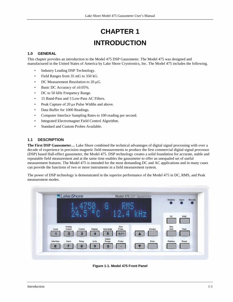
Figure 1-1. Model 475 Front Panel
Lake Shore Model 475 Gaussmeter User’s Manual
1-2 Introduction
DC Measurement Mode: Static or slowly changing fields are measured in DC mode where the accuracy, resolution, and stability of the Model 475 are most evident. The gaussmeter takes advantage of the internal auto zero function and probe linearity compensation to provide its best accuracy in this mode. Measurement resolution is enhanced by advanced signal processing capability, allowing users the choice of high reading rates (100 readings per second or more) or high resolution (to 5¾ digits in DC mode). The Model 475 also features front-end amplification that was specifically designed to complement DSP data acquisition to provide high stability and repeatability. That, along with probe temperature compensation, makes the Model 475 the most stable gaussmeter that Lake Shore has ever produced, suiting it perfectly for demanding DC measurement applications such as field mapping and field control. RMS Measurement Mode: Periodic AC fields are measured in RMS mode, which highlights the uniquely flexible filter functions of the Model 475. An overall frequency range of 1 Hz to 20 kHz is offered by the gaussmeter. Selectable band-pass and low-pass filters allow users to reject unwanted signals and improve measurement performance. Digital signal processing algorithms also free the Model 475 from the limitations of conventional RMS conversion hardware and provide better dynamic range, resolution, and frequency response than ever before. These improvements permit meaningful RMS field measurements with broad frequency content or in noisy environments. (Best high frequency performance requires proper probe selection.) Peak Measurement Mode: Pulsed fields are measured in Peak mode, which is a natural extension of the high-speed data acquisition necessary for DSP operation. Fast instrument sample rates permit capture of positive and negative field pulses as narrow as 20 µs in width, which can be held for an unlimited length of time with no sag. This is ideal for most magnetizers and other fast pulse applications. For more moderate field changes, the Model 475 can process the captured data to create other features. The gaussmeter can be configured to follow the peak of a periodic waveform for evaluation of crest factor. The Model 475 can also be used to sample field changes at 1000 readings per second that can later be read over interface to illustrate the shape of pulses or other waveforms. The Probe Connection: The Model 475 is only half of the magnetic field measurement equation. For the complete solution, Lake Shore offers a full complement of standard Hall-effect probes in a variety of sizes and sensitivities. The probes are designed and built at Lake Shore to provide the maximum benefit from the advanced features of the gaussmeter. Each probe is calibrated to compensate for both field and temperature effects. The calibration data is loaded into the probe connector for hassle free interchangeability including hot swapping. Three different probe sensitivities are available and extend full-scale measurement ranges from 35 mG to 350 kG. Custom probes are also available from Lake Shore when the standard configurations do not meet all application requirements.
1.1.1 Advanced Features In addition, the features that users have come to expect from Lake Shore gaussmeters, the Model 475 combines elements of hardware and firmware to create advanced features that facilitate automation and materials analysis. Field Control: A built in PI control algorithm turns the Model 475 into an essential building block for magnetic field control in electromagnet systems. The gaussmeter and a voltage programmable magnet power supply are all that is needed to control stable magnetic fields in an electromagnet at the user specified setpoint. One of the built in analog voltage outputs is used to drive the program input of the power supply for either bipolar or unipolar operation. High Speed Data Transfer: The IEEE-488 interface can be configured to send readings in binary format rather than the more common ASCII format. This reduces interface overhead enabling real time reading rates up to 100 readings per second. Temperature compensation is not available at the highest interface rate. Data Buffer: Memory within the instrument provides storage for 1024 field readings in a data buffer. The buffer can be filed at high speed, up to 1000 reading per second, which is as much as ten times faster than the computer interface. Stored readings can then be retrieved over interface at slower speed and processed off-line. Trigger input can be used to initiate the data log sequence. Slower sample rates can be programmed if desired. Trigger In and Trigger Out: A hardware, TTL level, trigger into the instrument can be used to initiate the data log sequence. A hardware, TTL level trigger out of the instrument indicates when the instrument completes a reading and can be used to synchronize other instrument in the system. A software, IEEE-488 based trigger can be used like the hardware trigger in.

Lake Shore Model 475 Gaussmeter User’s Manual
Introduction 1-3
1.1.2 Measurement Features The Model 475 offers a variety of features, implemented in the instrument firmware, to enhance usability and convenience of the gaussmeter. Auto Range: In addition to manual range selection, the instrument will automatically choose an appropriate range for the measured field. Auto range works in DC and AC measurement modes. Auto Probe Zero: Allows the user to zero all ranges for the selected measurement mode with the push of a key. Display Units: Field magnitude can be displayed in units of G, T, Oe, and A/m. Max/Min Hold: The instrument stores the fully processed maximum and minimum DC or RMS field value. This differs from the faster peak capture feature that operates on broadband, unprocessed field reading information. Relative Reading: Relative feature calculates the difference between a live reading and the relative setpoint to highlight deviation from a known field point. This feature can be used in DC, RMS, or Peak measurement mode. Instrument Calibration: Lake Shore recommends an annual recalibration schedule for all precision gaussmeters. Recalibrations are always available from the factory but the Model 475 allows users to field calibrate the instrument if necessary. Recalibration requires a working computer interface and precision low resistance standards of known value.
1.1.3 Probe Support The Model 475 has several capabilities that permit the best possible measurements with Lake Shore probes. These firmware-based features work in tandem with the calibration and programming of the probe to ensure accurate, repeatable measurements and ease of setup. Many of the features require probe characteristics that are stored in non-volatile memory located in the probe connector during calibration. Probe Field Compensation: The Hall-effect devices used in gaussmeter probes produce a near linear response in the presence of magnetic field. The small non-linearities present in each individual device can be measured and subtracted from the field reading. Model 475 probes are calibrated in this way to provide the most accurate DC readings. Probe Temperature Compensation: Hall-effect devices show a slight change in sensitivity and offset with temperature. A probes temperature effects can be measured and subtracted out of field readings. A temperature sensor, installed in the probe tip of Model 475 probes, relays real time temperature to the gaussmeter so that it can perform compensation. Although temperature effects contribute only a small fraction of the overall probe measurement accuracy, temperature compensation will often improve measurement and control stability. Probe Temperature Display: When using a probe that includes a temperature sensor, the gaussmeter can display the temperature of the probe in °C along with a field reading. Frequency Display: When operating in RMS mode, the gaussmeter can display the frequency of the measured AC field along with a field reading. Probe Information: The gaussmeter reads the probe information on power up or any time the probe is changed to allow hot swapping of probes. Critical probe information can be viewed on the front panel and read over computer interface to ensure proper system configuration. Extension Cables: The complex nature of Hall-effect measurements makes it necessary to match extension cables to the probe when longer cables are necessary. Keeping probes and their extensions from getting mixed up can become a problem when more than one probe is in use. The Model 475 alleviates some of the difficulty by allowing users to match probes to extensions in the field. Stored information can be viewed on the front panel and read over computer interface to ensure proper mating.
Lake Shore Model 475 Gaussmeter User’s Manual
1-4 Introduction
Probe Availability: Listed in Chapter 7 with specifications are some of the commonly used probes for the Model 475 gaussmeter. This is by no means the limit of what is offered. All probe physical configurations previously supplied with the 450 gaussmeter are available for the Model 475. The model number for Model 475 probes is identical, except an “H” has been added as the first character. Lake Shore prides itself on trying to satisfy every customer request for special probes. Hall Generators: The Model 475 will operate with a discrete hall generator when a suitable probe is not available. Users can program nominal sensitivity and serial number into a blank connector (HMCBL-6, ordered separately) to provide all gaussmeter functions except field and temperature compensation. If no sensitivity information is available, the Model 475 reverts to resistance measurement.
1.1.4 Display and Interface Features Display: The Model 475 has a two line by 20 character vacuum fluorescent display with 9mm high characters. During normal operation. the display is used to report field readings and give results of other features like max/min or relative. The display can also be configured to show probe temperature or frequency. When setting instrument parameters, the display gives the operator meaningful prompts and feedback to simplify operation. The operator can also control display brightness. Keypad: The instrument has a 22 position keypad with individual key assigned to frequently used features. Menus are reserved for less frequently used setup operations. The keypad can be locked out to prevent unintended changes of instrument setup. Alarm and Relay: High and low alarms are included in the instrument. Alarm actuators include display annunciator, audible beeper and two relays. The relays can also be controlled manually for other system needs. Voltage Output 1: The first voltage output gives access to amplified voltage signal directly from the probe. This voltage is corrected for the nominal sensitivity of the probe and provides the widest bandwidth of the three voltage outputs. In wideband AC mode, its signal can be viewed on an oscilloscope to observe the shape of AC fields. In peak mode the output can be used to view pulse shape or other characteristic of a momentary signal. Output 1 serves only as a diagnostic tool in DC and narrow band AC modes because the intrinsic modulation of the probe signal prevents a clear view of the field response. Voltage Output 2: The second voltage output provides a voltage proportional to measured field with the benefits of some signal processing. The output is produced by the DSP through a fast D/A converter. The output signal is updated at 40 kHz, giving good response for low to mid frequency fields. Signal quality degrades at high frequency because of the sampling rate. Probe offset correction and correction for the nominal sensitivity of the probe can be performed on this signal. Voltage Output 3: The third voltage output provides a voltage proportional to measured field with the most signal processing of the three outputs. All probe compensation available to the display readings, including temperature compensation, can be performed on this output. The output is produced by the microprocessor through a high-resolution, 16-bit, D/A converter updated at 30 readings per second. This output can also be used for field control. Computer Interface: Two computer interfaces are included with the Model 475, serial RS-232C and parallel IEEE-488. Both allow setup of all instrument parameters and read-back of measured values. The reading rate over interface is nominally 30 readings per second but ranges from 10 to 100 readings per second depending on setup. Lake Shore makes LabView drivers available to its instrument users, consult factory for availability.
Lake Shore Model 475 Gaussmeter User’s Manual
Introduction 1-5
1.2 SPECIFICATIONS Full specifications about the Model 475 gaussmeter are provided on our website. Please see: http://www.lakeshore.com/products/gaussmeters/model-475-dsp-gaussmeter/pages/Specifications.aspx. 1.3 SAFETY SUMMARY Observe these general safety precautions during all phases of instrument operation, service, and repair. Failure to comply with these precautions or with specific warnings elsewhere in this manual violates safety standards of design, manufacture, and intended instrument use. Lake Shore Cryotronics, Inc. assumes no liability for Customer failure to comply with these requirements.
The Model 475 protects the operator and surrounding area from electric shock or burn, mechanical hazards, excessive temperature, and spread of fire from the instrument. Environmental conditions outside of the conditions below may pose a hazard to the operator and surrounding area.
• Indoor use. • Altitude to 2000 meters. • Temperature for safe operation: 5 °C to 40 °C. • Maximum relative humidity: 80% for temperature up to 31 °C decreasing linearly to 50% at 40 °C. • Power supply voltage fluctuations not to exceed ±10% of the nominal voltage. • Overvoltage category II. • Pollution degree 2. Ground the Instrument
To minimize shock hazard, the instrument is equipped with a 3-conductor AC power cable. Plug the power cable into an approved three-contact electrical outlet or use a three-contact adapter with the grounding wire (green) firmly connected to an electrical ground (safety ground) at the power outlet. The power jack and mating plug of the power cable meet Underwriters Laboratories (UL) and International Electrotechnical Commission (IEC) safety standards.
Ventilation The instrument has ventilation holes in its side covers. Do not block these holes when the instrument is operating.
Do Not Operate in An Explosive Atmosphere Do not operate the instrument in the presence of flammable gases or fumes. Operation of any electrical instrument in such an environment constitutes a definite safety hazard.
Keep Away from Live Circuits Operating personnel must not remove instrument covers. Refer component replacement and internal adjustments to qualified maintenance personnel. Do not replace components with power cable connected. To avoid injuries, always disconnect power and discharge circuits before touching them.
Do Not Substitute Parts or Modify Instrument Do not install substitute parts or perform any unauthorized modification to the instrument. Return the instrument to an authorized Lake Shore Cryotronics representative for service and repair to ensure that safety features are maintained.
Cleaning Do not submerge instrument. Clean only with a damp cloth and mild detergent. Exterior only.

Lake Shore Model 475 Gaussmeter User’s Manual
1-6 Introduction
1.4 SAFETY SYMBOLS
Lake Shore Model 475 Gaussmeter User’s Manual
Background 2-1
CHAPTER 2
BACKGROUND
2.0 GENERAL This chapter provides background information related to the Model 475 Gaussmeter. It is intended to give the user insight into the benefits and limitations of the instrument and help apply the features of the Model 475 to a variety of experimental challenges. It covers basic DSP concepts and how they are applied to the operation of the Model 475, flux density and Hall measurement, probe operation, and an introduction to field control. For information on how to install the Model 475 please refer to Chapter 3. Instrument operation information is contained in Chapter 4 and Chapter 5.
2.1 MODEL 475 THEORY OF OPERATION
2.1.1 Sampled Data Systems Humans rely on analog signals to interact with their environment: individual wavelengths of light are converted to colors, pressure waves are interpreted as sound, and the vibration of vocal cords creates speech. In the fields of science and engineering, a variety of sensors are used to convert analog signals of interest into some electrical property, usually voltage, so that they can be measured or used as an input to a system. Analog-to-digital converters (ADC) and digital-to-analog converters (DAC) allow computers in the digital domain to interact with these analog signals. Digital signals are different from continuous analog signals in the fact that they are sampled in time and quantized in amplitude. Both of these properties limit the ability of the digital representation to match the original analog signal. An ADC will sample a signal at fixed intervals of time. Quantization results from the fact that an ADC has a limited amount of resolution. When both the sampling frequency and resolution are properly chosen however, the digital signal is an accurate representation of the original analog signal. The sampling frequency of the Model 475 allows an accurate RMS measurement to be made on signals of up to 20 kHz. The sampling and filtering in the Model 475 can allow realizable resolutions of 20 bits, which is in the noise floor of the instrument.
2.1.2 Digital Signal Processing Digital Signal Processing (DSP) is the science of manipulating digital data through the use of mathematics. The variety of processing that can be done is almost endless, from simulating an analog filter, to enhancing a visual image, to encrypting sensitive information. Digital Signal Processing is being used in more and more products due to its accuracy, flexibility, and reliability. The Model 475 Gaussmeter is an ideal product that can benefit from DSP technology. The Model 475 offers the user a choice of 15 band-pass and 3 low-pass AC filters. Digital filters can easily be modified in software and in addition offer a sharper roll-off, less ripple in the pass-band, and better stop-band attenuation. It would be difficult to implement all of these filters in an analog form since changing the filter parameters would require extensive hardware manipulation. The components that are used in analog signal processing can have different values from component to component and are temperature dependent. Using Digital Signal Processing gives better measurement repeatability and increases the temperature stability of the instrument.
2.1.3 Limitations of Sampled Data Systems Sampled data systems do have their limitations, but if they are understood, they can be dealt with easily. The limitations of sampled data systems come from the fact that a continuous analog signal is being sampled and digitized. This inherently limits the frequency of the signal that can be read as well as the resolution at which it can be read. Typically, the resolution is high enough and enough averaging is done that it does not present a problem. The frequency limitation can cause unique problems. There are notches in the frequency response as the input signal approaches one-half the sampling rate and its harmonics. As the measured signal approaches these harmonic frequencies, the reading will fall off due to the null in the filter.
Lake Shore Model 475 Gaussmeter User’s Manual
2-2 Background
The rate at which an analog signal must be sampled depends on the frequency content of the signal. A signal is said to be properly sampled if the original signal can be exactly reconstructed from the digital information. It turns out that a signal can only be properly reconstructed if the signal does not contain frequencies above one-half of the sampling rate. This is referred to as the Nyquist frequency. In the case of the Model 475, the ADC is sampled at 40 kHz in wide band AC mode. In this mode, the highest frequency signal that can be accurately represented out of Analog Output 2 is 20 kHz due to the limit of the Nyquist frequency. In this case, Analog Output 1 should be used to monitor the signal. It should be noted that although the Nyquist frequency will limit the signal that can be accurately reconstructed, it doesn’t affect the RMS reading of the signal. The energy content of the signal above the Nyquist frequency will be aliased to lower frequencies where it will be included in the RMS calculation.
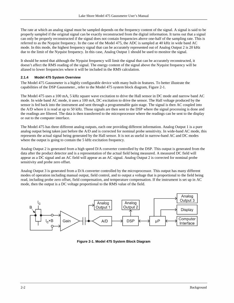
2.1.4 Model 475 System Overview The Model 475 Gaussmeter is a highly configurable device with many built-in features. To better illustrate the capabilities of the DSP Gaussmeter., refer to the Model 475 system block diagram, Figure 2-1. The Model 475 uses a 100 mA, 5 kHz square wave excitation to drive the Hall sensor in DC mode and narrow band AC mode. In wide band AC mode, it uses a 100 mA, DC excitation to drive the sensor. The Hall voltage produced by the sensor is fed back into the instrument and sent through a programmable gain stage. The signal is then AC coupled into the A/D where it is read at up to 50 kHz. Those signals are then sent to the DSP where the signal processing is done and the readings are filtered. The data is then transferred to the microprocessor where the readings can be sent to the display or out to the computer interface. The Model 475 has three different analog outputs, each one providing different information. Analog Output 1 is a pure analog output being taken just before the A/D and is corrected for nominal probe sensitivity. In wide-band AC mode, this represents the actual signal being generated by the Hall sensor. It is not as useful in narrow-band AC and DC modes where the output is going to contain the 5 kHz excitation frequency. Analog Output 2 is generated from a high speed D/A converter controlled by the DSP. This output is generated from the data after the product detector and is a representation of the actual field being measured. A measured DC field will appear as a DC signal and an AC field will appear as an AC signal. Analog Output 2 is corrected for nominal probe sensitivity and probe zero offset. Analog Output 3 is generated from a D/A converter controlled by the microprocessor. This output has many different modes of operation including manual output, field control, and to output a voltage that is proportional to the field being read, including probe zero offset, field compensation, and temperature compensation. If the instrument is set up in AC mode, then the output is a DC voltage proportional to the RMS value of the field.
Figure 2-1. Model 475 System Block Diagram
Lake Shore Model 475 Gaussmeter User’s Manual
Background 2-3
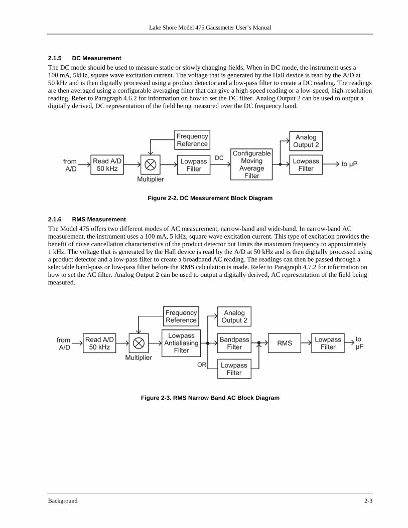
2.1.5 DC Measurement The DC mode should be used to measure static or slowly changing fields. When in DC mode, the instrument uses a 100 mA, 5kHz, square wave excitation current. The voltage that is generated by the Hall device is read by the A/D at 50 kHz and is then digitally processed using a product detector and a low-pass filter to create a DC reading. The readings are then averaged using a configurable averaging filter that can give a high-speed reading or a low-speed, high-resolution reading. Refer to Paragraph 4.6.2 for information on how to set the DC filter. Analog Output 2 can be used to output a digitally derived, DC representation of the field being measured over the DC frequency band.
Figure 2-2. DC Measurement Block Diagram
2.1.6 RMS Measurement The Model 475 offers two different modes of AC measurement, narrow-band and wide-band. In narrow-band AC measurement, the instrument uses a 100 mA, 5 kHz, square wave excitation current. This type of excitation provides the benefit of noise cancellation characteristics of the product detector but limits the maximum frequency to approximately 1 kHz. The voltage that is generated by the Hall device is read by the A/D at 50 kHz and is then digitally processed using a product detector and a low-pass filter to create a broadband AC reading. The readings can then be passed through a selectable band-pass or low-pass filter before the RMS calculation is made. Refer to Paragraph 4.7.2 for information on how to set the AC filter. Analog Output 2 can be used to output a digitally derived, AC representation of the field being measured.
Figure 2-3. RMS Narrow Band AC Block Diagram
Lake Shore Model 475 Gaussmeter User’s Manual
2-4 Background
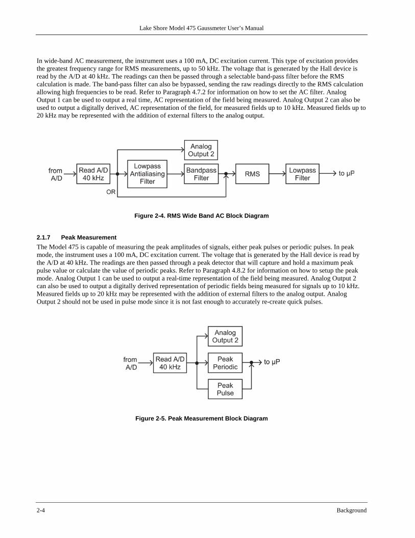
In wide-band AC measurement, the instrument uses a 100 mA, DC excitation current. This type of excitation provides the greatest frequency range for RMS measurements, up to 50 kHz. The voltage that is generated by the Hall device is read by the A/D at 40 kHz. The readings can then be passed through a selectable band-pass filter before the RMS calculation is made. The band-pass filter can also be bypassed, sending the raw readings directly to the RMS calculation allowing high frequencies to be read. Refer to Paragraph 4.7.2 for information on how to set the AC filter. Analog Output 1 can be used to output a real time, AC representation of the field being measured. Analog Output 2 can also be used to output a digitally derived, AC representation of the field, for measured fields up to 10 kHz. Measured fields up to 20 kHz may be represented with the addition of external filters to the analog output.
Figure 2-4. RMS Wide Band AC Block Diagram
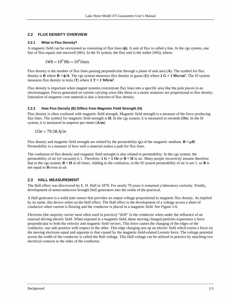
2.1.7 Peak Measurement The Model 475 is capable of measuring the peak amplitudes of signals, either peak pulses or periodic pulses. In peak mode, the instrument uses a 100 mA, DC excitation current. The voltage that is generated by the Hall device is read by the A/D at 40 kHz. The readings are then passed through a peak detector that will capture and hold a maximum peak pulse value or calculate the value of periodic peaks. Refer to Paragraph 4.8.2 for information on how to setup the peak mode. Analog Output 1 can be used to output a real-time representation of the field being measured. Analog Output 2 can also be used to output a digitally derived representation of periodic fields being measured for signals up to 10 kHz. Measured fields up to 20 kHz may be represented with the addition of external filters to the analog output. Analog Output 2 should not be used in pulse mode since it is not fast enough to accurately re-create quick pulses.
Figure 2-5. Peak Measurement Block Diagram
Lake Shore Model 475 Gaussmeter User’s Manual
Background 2-5
2.2 FLUX DENSITY OVERVIEW
2.2.1 What is Flux Density? A magnetic field can be envisioned as consisting of flux lines (φ). A unit of flux is called a line. In the cgs system, one line of flux equals one maxwell (Mx). In the SI system, the flux unit is the weber (Wb), where:
8 81 10 10 .Wb Mx lines= = Flux density is the number of flux lines passing perpendicular through a plane of unit area (A). The symbol for flux density is B where B = φ/A. The cgs system measures flux density in gauss (G) where 1 G = 1 Mx/cm2. The SI system measures flux density in tesla (T) where 1 T = 1 Wb/m2. Flux density is important when magnet systems concentrate flux lines into a specific area like the pole pieces in an electromagnet. Forces generated on current carrying wires like those in a motor armature are proportional to flux density. Saturation of magnetic core material is also a function of flux density.
2.2.2 How Flux Density (B) Differs from Magnetic Field Strength (H) Flux density is often confused with magnetic field strength. Magnetic field strength is a measure of the force producing flux lines. The symbol for magnetic field strength is H. In the cgs system, it is measured in oersteds (Oe). In the SI system, it is measured in amperes per meter (A/m):
1 79.58Oe A m= . Flux density and magnetic field strength are related by the permeability (µ) of the magnetic medium. B = µH. Permeability is a measure of how well a material makes a path for flux lines. The confusion of flux density and magnetic field strength is also related to permeability. In the cgs system, the permeability of air (of vacuum) is 1. Therefore, 1 G = 1 Oe or B = H in air. Many people incorrectly assume therefore that in the cgs system, B = H at all times. Adding to the confusion, in the SI system permeability of air is not 1, so B is not equal to H even in air.
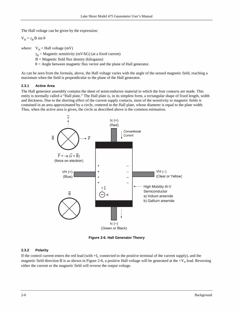
2.3 HALL MEASUREMENT The Hall effect was discovered by E. H. Hall in 1879. For nearly 70 years it remained a laboratory curiosity. Finally, development of semiconductors brought Hall generators into the realm of the practical. A Hall generator is a solid state sensor that provides an output voltage proportional to magnetic flux density. As implied by its name, this device relies on the Hall effect. The Hall effect is the development of a voltage across a sheet of conductor when current is flowing and the conductor is placed in a magnetic field. See Figure 2-6. Electrons (the majority carrier most often used in practice) “drift” in the conductor when under the influence of an external driving electric field. When exposed to a magnetic field, these moving charged particles experience a force perpendicular to both the velocity and magnetic field vectors. This force causes the charging of the edges of the conductor, one side positive with respect to the other. This edge charging sets up an electric field which exerts a force on the moving electrons equal and opposite to that caused by the magnetic-field-related Lorentz force. The voltage potential across the width of the conductor is called the Hall voltage. This Hall voltage can be utilized in practice by attaching two electrical contacts to the sides of the conductor.
Lake Shore Model 475 Gaussmeter User’s Manual
2-6 Background
The Hall voltage can be given by the expression:
VH = γB B sin θ where: VH = Hall voltage (mV) γB = Magnetic sensitivity (mV/kG) (at a fixed current) B = Magnetic field flux density (kilogauss) θ = Angle between magnetic flux vector and the plane of Hall generator. As can be seen from the formula, above, the Hall voltage varies with the angle of the sensed magnetic field, reaching a maximum when the field is perpendicular to the plane of the Hall generator.
2.3.1 Active Area The Hall generator assembly contains the sheet of semiconductor material to which the four contacts are made. This entity is normally called a “Hall plate.” The Hall plate is, in its simplest form, a rectangular shape of fixed length, width and thickness. Due to the shorting effect of the current supply contacts, most of the sensitivity to magnetic fields is contained in an area approximated by a circle, centered in the Hall plate, whose diameter is equal to the plate width. Thus, when the active area is given, the circle as described above is the common estimation.
Figure 2-6. Hall Generator Theory
2.3.2 Polarity If the control current enters the red lead (with +IC connected to the positive terminal of the current supply), and the magnetic field direction B is as shown in Figure 2-6, a positive Hall voltage will be generated at the +VH lead. Reversing either the current or the magnetic field will reverse the output voltage.
Lake Shore Model 475 Gaussmeter User’s Manual
Background 2-7
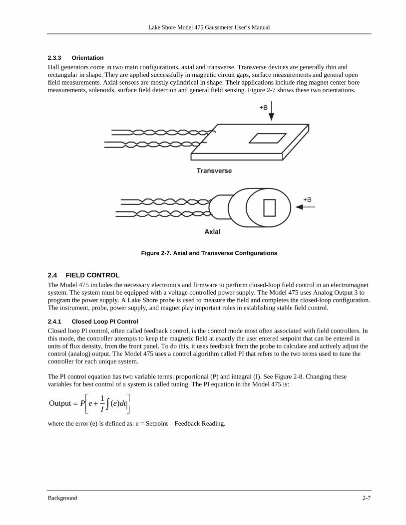
2.3.3 Orientation Hall generators come in two main configurations, axial and transverse. Transverse devices are generally thin and rectangular in shape. They are applied successfully in magnetic circuit gaps, surface measurements and general open field measurements. Axial sensors are mostly cylindrical in shape. Their applications include ring magnet center bore measurements, solenoids, surface field detection and general field sensing. Figure 2-7 shows these two orientations.
Figure 2-7. Axial and Transverse Configurations
2.4 FIELD CONTROL The Model 475 includes the necessary electronics and firmware to perform closed-loop field control in an electromagnet system. The system must be equipped with a voltage controlled power supply. The Model 475 uses Analog Output 3 to program the power supply. A Lake Shore probe is used to measure the field and completes the closed-loop configuration. The instrument, probe, power supply, and magnet play important roles in establishing stable field control.
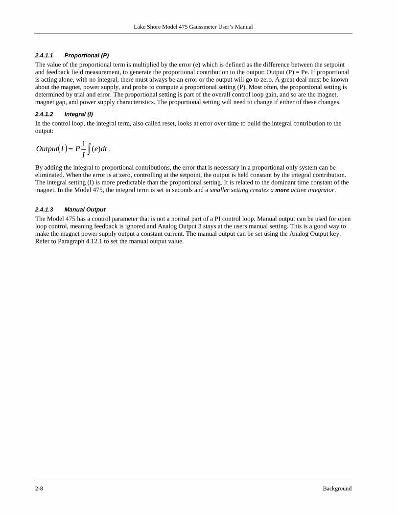
2.4.1 Closed Loop PI Control Closed loop PI control, often called feedback control, is the control mode most often associated with field controllers. In this mode, the controller attempts to keep the magnetic field at exactly the user entered setpoint that can be entered in units of flux density, from the front panel. To do this, it uses feedback from the probe to calculate and actively adjust the control (analog) output. The Model 475 uses a control algorithm called PI that refers to the two terms used to tune the controller for each unique system. The PI control equation has two variable terms: proportional (P) and integral (I). See Figure 2-8. Changing these variables for best control of a system is called tuning. The PI equation in the Model 475 is:
+= ∫ dte
IeP )(1Output
where the error (e) is defined as: e = Setpoint – Feedback Reading.
Lake Shore Model 475 Gaussmeter User’s Manual
2-8 Background
2.4.1.1 Proportional (P) The value of the proportional term is multiplied by the error (e) which is defined as the difference between the setpoint and feedback field measurement, to generate the proportional contribution to the output: Output (P) = Pe. If proportional is acting alone, with no integral, there must always be an error or the output will go to zero. A great deal must be known about the magnet, power supply, and probe to compute a proportional setting (P). Most often, the proportional setting is determined by trial and error. The proportional setting is part of the overall control loop gain, and so are the magnet, magnet gap, and power supply characteristics. The proportional setting will need to change if either of these changes.
2.4.1.2 Integral (I) In the control loop, the integral term, also called reset, looks at error over time to build the integral contribution to the output:
( ) ∫= dteI
PIOutput )(1.
By adding the integral to proportional contributions, the error that is necessary in a proportional only system can be eliminated. When the error is at zero, controlling at the setpoint, the output is held constant by the integral contribution. The integral setting (I) is more predictable than the proportional setting. It is related to the dominant time constant of the magnet. In the Model 475, the integral term is set in seconds and a smaller setting creates a more active integrator.
2.4.1.3 Manual Output The Model 475 has a control parameter that is not a normal part of a PI control loop. Manual output can be used for open loop control, meaning feedback is ignored and Analog Output 3 stays at the users manual setting. This is a good way to make the magnet power supply output a constant current. The manual output can be set using the Analog Output key. Refer to Paragraph 4.12.1 to set the manual output value.
Lake Shore Model 475 Gaussmeter User’s Manual
Background 2-9
Figure 2-8. Examples of PI Control

Lake Shore Model 475 Gaussmeter User’s Manual
2-10 Background
2.4.2 Tuning a Closed Loop PI Controller There has been a lot written about tuning closed loop control systems and specifically PI control loops. This section does not attempt to compete with control theory experts. It describes a few basic rules of thumb to help less experienced users get started. This technique will not solve every problem, but it has worked for many others in the field. This section assumes the user has worked through the operation sections of this manual. Be sure to setup the Control Slope Limit and the Analog Output Voltage Limit before attempting to tune the field control system. This will assure that the magnet power supply will not be damaged if the field control system is improperly tuned or begins to oscillate. Refer to Paragraph 5.3 to setup field control. Also, begin control with the DC filter set to 3 or 4 digits of resolution. Since the field control works on the filtered readings, it becomes difficult to control the system with the added time constant from the slow filtering on the 5 digit setting.
2.4.2.1 Tuning Proportional The proportional setting is tied to the overall gain of the system. The gain of the power supply should be fairly constant over its entire range of operation but the gain of the magnet changes with field. As the magnet approaches saturation, the amount of current needed to change the field a given amount increases substantially. No single value of P will be sufficient to maintain acceptable control over the entire range of magnet operation. To find the correct proportional setting for a system, turn off the I setting and start with a low value for P, approximately 5 or 10. Set the control setpoint to some low, non-zero field, 1 kG for example. If the field is oscillating, then P is too high and needs to be reduced. If the field is not oscillating, increase P by a factor of two until the system begins to oscillate. See Figure 2-8(a). Do not set the proportional setting so high that it causes violent oscillations. The appropriate value for P is one half of the value required for sustained oscillation. An even lower setting of one quarter may be desired for minimal overshoot. See Figure 2-8(b).
2.4.2.2 Tuning Integral When the proportional setting is chosen and the integral is turned off, the Model 475 will control the field to some value below the setpoint. Setting the integral allows the Model 475 control algorithm to gradually eliminate the difference in field by integrating the error over time. See Figure 2-8(d). An integral setting that is too low causes the field to take too long to reach the setpoint. An integral setting that is too high can create overshoot, which cannot be tolerated in many magnetic systems. An integral setting that is very high will eventually cause the field to oscillate. Begin this part of the tuning process using the proportional setting found above. Enter an I setting of 100 to start with. If the field begins to oscillate, increase the I setting by a factor of two. Remember, in the Model 475, the integral term is set in seconds and a smaller setting creates a more active integrator. If the field is stable but never reaches the setpoint, the integral setting is too high and should be reduced by one half. To verify the integral setting, make a few small (1 kG) changes in setpoint and watch the field react. Trial and error can help improve the integral setting by optimizing for experimental needs. Faster integrals, for example, get to the setpoint more quickly at the expense of greater overshoot.
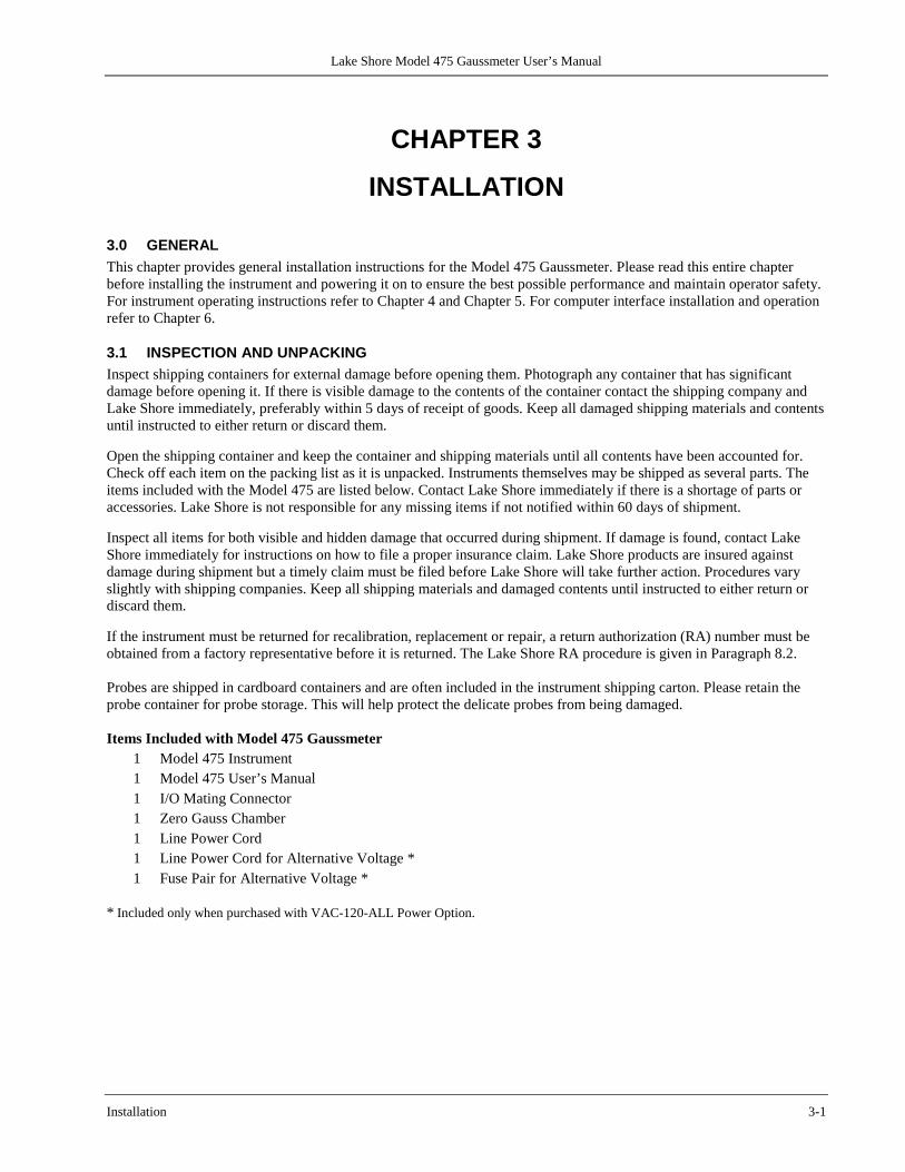
Lake Shore Model 475 Gaussmeter User’s Manual
Installation 3-1
CHAPTER 3
INSTALLATION
3.0 GENERAL This chapter provides general installation instructions for the Model 475 Gaussmeter. Please read this entire chapter before installing the instrument and powering it on to ensure the best possible performance and maintain operator safety. For instrument operating instructions refer to Chapter 4 and Chapter 5. For computer interface installation and operation refer to Chapter 6.
3.1 INSPECTION AND UNPACKING Inspect shipping containers for external damage before opening them. Photograph any container that has significant damage before opening it. If there is visible damage to the contents of the container contact the shipping company and Lake Shore immediately, preferably within 5 days of receipt of goods. Keep all damaged shipping materials and contents until instructed to either return or discard them. Open the shipping container and keep the container and shipping materials until all contents have been accounted for. Check off each item on the packing list as it is unpacked. Instruments themselves may be shipped as several parts. The items included with the Model 475 are listed below. Contact Lake Shore immediately if there is a shortage of parts or accessories. Lake Shore is not responsible for any missing items if not notified within 60 days of shipment. Inspect all items for both visible and hidden damage that occurred during shipment. If damage is found, contact Lake Shore immediately for instructions on how to file a proper insurance claim. Lake Shore products are insured against damage during shipment but a timely claim must be filed before Lake Shore will take further action. Procedures vary slightly with shipping companies. Keep all shipping materials and damaged contents until instructed to either return or discard them. If the instrument must be returned for recalibration, replacement or repair, a return authorization (RA) number must be obtained from a factory representative before it is returned. The Lake Shore RA procedure is given in Paragraph 8.2. Probes are shipped in cardboard containers and are often included in the instrument shipping carton. Please retain the probe container for probe storage. This will help protect the delicate probes from being damaged. Items Included with Model 475 Gaussmeter
1 Model 475 Instrument 1 Model 475 User’s Manual 1 I/O Mating Connector 1 Zero Gauss Chamber 1 Line Power Cord 1 Line Power Cord for Alternative Voltage * 1 Fuse Pair for Alternative Voltage *
* Included only when purchased with VAC-120-ALL Power Option.
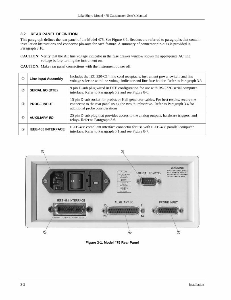
Lake Shore Model 475 Gaussmeter User’s Manual
3-2 Installation
3.2 REAR PANEL DEFINITION This paragraph defines the rear panel of the Model 475. See Figure 3-1. Readers are referred to paragraphs that contain installation instructions and connector pin-outs for each feature. A summary of connector pin-outs is provided in Paragraph 8.10. CAUTION: Verify that the AC line voltage indicator in the fuse drawer window shows the appropriate AC line
voltage before turning the instrument on. CAUTION: Make rear panel connections with the instrument power off.
Line Input Assembly Includes the IEC 320-C14 line cord receptacle, instrument power switch, and line voltage selector with line voltage indicator and line fuse holder. Refer to Paragraph 3.3.
SERIAL I/O (DTE) 9 pin D-sub plug wired in DTE configuration for use with RS-232C serial computer interface. Refer to Paragraph 6.2 and see Figure 8-6.
PROBE INPUT 15 pin D-sub socket for probes or Hall generator cables. For best results, secure the connector to the rear panel using the two thumbscrews. Refer to Paragraph 3.4 for additional probe considerations.
AUXILIARY I/O 25 pin D-sub plug that provides access to the analog outputs, hardware triggers, and relays. Refer to Paragraph 3.6.
IEEE-488 INTERFACE IEEE-488 compliant interface connector for use with IEEE-488 parallel computer interface. Refer to Paragraph 6.1 and see Figure 8-7.
Figure 3-1. Model 475 Rear Panel
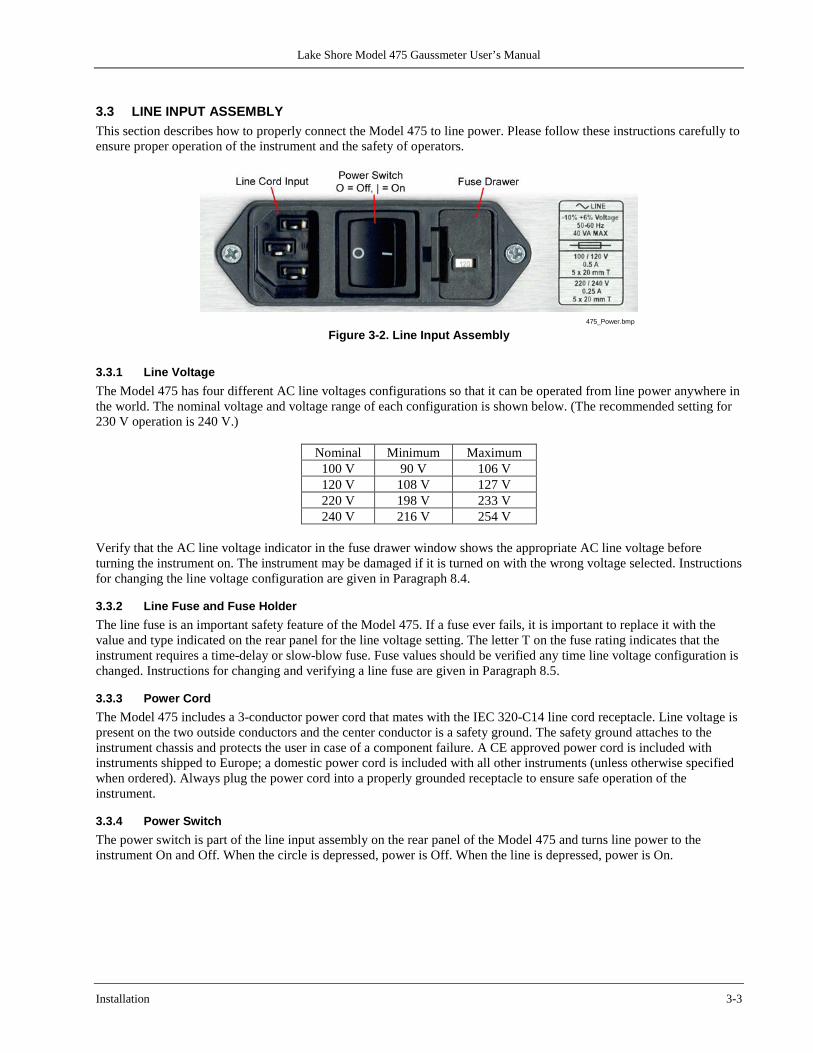
Lake Shore Model 475 Gaussmeter User’s Manual
Installation 3-3
3.3 LINE INPUT ASSEMBLY This section describes how to properly connect the Model 475 to line power. Please follow these instructions carefully to ensure proper operation of the instrument and the safety of operators.
475_Power.bmp
Figure 3-2. Line Input Assembly
3.3.1 Line Voltage The Model 475 has four different AC line voltages configurations so that it can be operated from line power anywhere in the world. The nominal voltage and voltage range of each configuration is shown below. (The recommended setting for 230 V operation is 240 V.)
Nominal Minimum Maximum 100 V 90 V 106 V 120 V 108 V 127 V 220 V 198 V 233 V 240 V 216 V 254 V
Verify that the AC line voltage indicator in the fuse drawer window shows the appropriate AC line voltage before turning the instrument on. The instrument may be damaged if it is turned on with the wrong voltage selected. Instructions for changing the line voltage configuration are given in Paragraph 8.4.
3.3.2 Line Fuse and Fuse Holder The line fuse is an important safety feature of the Model 475. If a fuse ever fails, it is important to replace it with the value and type indicated on the rear panel for the line voltage setting. The letter T on the fuse rating indicates that the instrument requires a time-delay or slow-blow fuse. Fuse values should be verified any time line voltage configuration is changed. Instructions for changing and verifying a line fuse are given in Paragraph 8.5.
3.3.3 Power Cord The Model 475 includes a 3-conductor power cord that mates with the IEC 320-C14 line cord receptacle. Line voltage is present on the two outside conductors and the center conductor is a safety ground. The safety ground attaches to the instrument chassis and protects the user in case of a component failure. A CE approved power cord is included with instruments shipped to Europe; a domestic power cord is included with all other instruments (unless otherwise specified when ordered). Always plug the power cord into a properly grounded receptacle to ensure safe operation of the instrument.
3.3.4 Power Switch The power switch is part of the line input assembly on the rear panel of the Model 475 and turns line power to the instrument On and Off. When the circle is depressed, power is Off. When the line is depressed, power is On.
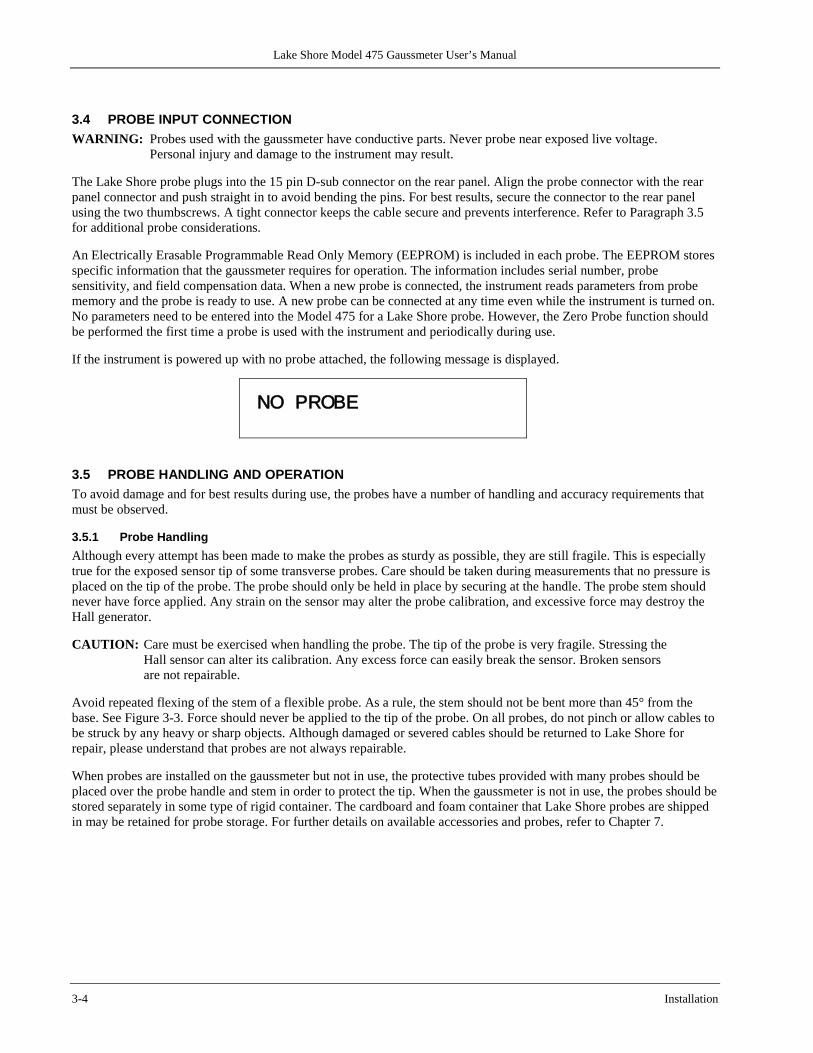
Lake Shore Model 475 Gaussmeter User’s Manual
3-4 Installation
3.4 PROBE INPUT CONNECTION WARNING: Probes used with the gaussmeter have conductive parts. Never probe near exposed live voltage.
Personal injury and damage to the instrument may result. The Lake Shore probe plugs into the 15 pin D-sub connector on the rear panel. Align the probe connector with the rear panel connector and push straight in to avoid bending the pins. For best results, secure the connector to the rear panel using the two thumbscrews. A tight connector keeps the cable secure and prevents interference. Refer to Paragraph 3.5 for additional probe considerations. An Electrically Erasable Programmable Read Only Memory (EEPROM) is included in each probe. The EEPROM stores specific information that the gaussmeter requires for operation. The information includes serial number, probe sensitivity, and field compensation data. When a new probe is connected, the instrument reads parameters from probe memory and the probe is ready to use. A new probe can be connected at any time even while the instrument is turned on. No parameters need to be entered into the Model 475 for a Lake Shore probe. However, the Zero Probe function should be performed the first time a probe is used with the instrument and periodically during use. If the instrument is powered up with no probe attached, the following message is displayed.
NO PROBE
3.5 PROBE HANDLING AND OPERATION To avoid damage and for best results during use, the probes have a number of handling and accuracy requirements that must be observed.
3.5.1 Probe Handling Although every attempt has been made to make the probes as sturdy as possible, they are still fragile. This is especially true for the exposed sensor tip of some transverse probes. Care should be taken during measurements that no pressure is placed on the tip of the probe. The probe should only be held in place by securing at the handle. The probe stem should never have force applied. Any strain on the sensor may alter the probe calibration, and excessive force may destroy the Hall generator. CAUTION: Care must be exercised when handling the probe. The tip of the probe is very fragile. Stressing the
Hall sensor can alter its calibration. Any excess force can easily break the sensor. Broken sensors are not repairable.
Avoid repeated flexing of the stem of a flexible probe. As a rule, the stem should not be bent more than 45° from the base. See Figure 3-3. Force should never be applied to the tip of the probe. On all probes, do not pinch or allow cables to be struck by any heavy or sharp objects. Although damaged or severed cables should be returned to Lake Shore for repair, please understand that probes are not always repairable. When probes are installed on the gaussmeter but not in use, the protective tubes provided with many probes should be placed over the probe handle and stem in order to protect the tip. When the gaussmeter is not in use, the probes should be stored separately in some type of rigid container. The cardboard and foam container that Lake Shore probes are shipped in may be retained for probe storage. For further details on available accessories and probes, refer to Chapter 7.

Lake Shore Model 475 Gaussmeter User’s Manual
Installation 3-5
Figure 3-3. Maximum Flexible Probe Bend Radius
3.5.2 Probe Operation In the DC mode of operation, the orientation of the probe affects the polarity reading of the gaussmeter. On a transverse probe, the Lake Shore name printed on the handle indicates the side for positive (+) flux entry. On an axial probe, positive (+) flux entry is always from the front of the probe. See Figure 3-4. NOTE: For best results, the instrument and probe should warm up for at least 5 minutes before zeroing the probe,
and at least 30 minutes for rated accuracy. The probe and the zero gauss chamber should be at the same temperature.
If the exact direction of the magnetic field is unknown, the proper magnitude is determined by turning on Max Hold and slowly adjusting the probe. As the probe turns and the measured field rises and falls, its maximum value is held on the display. Make note of the probe orientation at the maximum reading to identify the field orientation.
Figure 3-4. Probe Orientation for Positive Measurement

Lake Shore Model 475 Gaussmeter User’s Manual
3-6 Installation
3.5.3 Probe Accuracy Considerations The user must consider all the possible contributors to the accuracy of the reading. Both the probe and gaussmeter have accuracy specifications that may impact the actual reading. The probe should be zeroed before making critical measurements. The zero probe function is used to null (cancel) out the zero offset of the probe or small magnetic fields. It is normally used in conjunction with the zero gauss chamber, but may also be used with an open probe (registering the local earth magnetic field). Users wishing to cancel out large magnetic fields should use the Relative function. Refer to Paragraph 4.6.6. Probe temperature can also affect readings. Refer to the two separate temperature coefficients listed on the specification sheet. The High Stability (HST) probes exhibit a low temperature coefficient of gain due to the inherent thermal stability of the materials used in its construction. Probe readings are dependent on the angle of the sensor (Hall sensor) in relation to the magnetic field. Maximum output occurs when the flux vector is perpendicular to the plane of the sensor. This is the condition that exists during factory calibration. The greater the deviation from orthogonality (from right angles in either of three axes), the larger the error of the reading. For example, a 5° variance on any one axis causes a 0.4% error, a 10° misalignment induces a 1.5% error, etc. See Figure 3-5. Tolerance of instrument, probe, and magnet must be considered for making critical measurements. The accuracy of the gaussmeter reading is typically ±0.05% of reading and ±0.005% of range, but the absolute accuracy readings for gaussmeters and Hall probes is a difficult specification to give, because all the variables of the measurement are difficult to reproduce. Differences in alignment and positioning will degrade measurement accuracy and repeatability. Finally, the best probes have an accuracy of ±0.10%. This implies that the absolute accuracy of a magnetic field measurement will not reliably be better than ±0.10% of reading, and is likely to be 0.20%.
Figure 3-5. Effect of Angle on Measurements
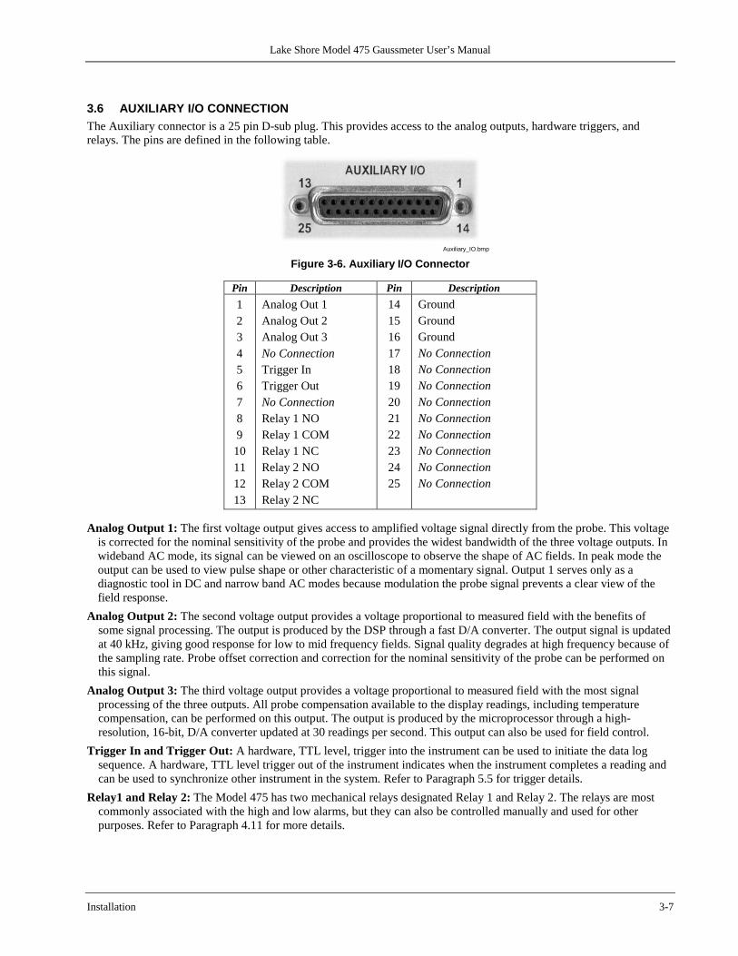
Lake Shore Model 475 Gaussmeter User’s Manual
Installation 3-7
3.6 AUXILIARY I/O CONNECTION The Auxiliary connector is a 25 pin D-sub plug. This provides access to the analog outputs, hardware triggers, and relays. The pins are defined in the following table.
Auxiliary_IO.bmp
Figure 3-6. Auxiliary I/O Connector
Pin Description Pin Description 1 2 3 4 5 6 7 8 9 10 11 12 13
Analog Out 1 Analog Out 2 Analog Out 3 No Connection Trigger In Trigger Out No Connection Relay 1 NO Relay 1 COM Relay 1 NC Relay 2 NO Relay 2 COM Relay 2 NC
14 15 16 17 18 19 20 21 22 23 24 25
Ground Ground Ground No Connection No Connection No Connection No Connection No Connection No Connection No Connection No Connection No Connection
Analog Output 1: The first voltage output gives access to amplified voltage signal directly from the probe. This voltage
is corrected for the nominal sensitivity of the probe and provides the widest bandwidth of the three voltage outputs. In wideband AC mode, its signal can be viewed on an oscilloscope to observe the shape of AC fields. In peak mode the output can be used to view pulse shape or other characteristic of a momentary signal. Output 1 serves only as a diagnostic tool in DC and narrow band AC modes because modulation the probe signal prevents a clear view of the field response.
Analog Output 2: The second voltage output provides a voltage proportional to measured field with the benefits of some signal processing. The output is produced by the DSP through a fast D/A converter. The output signal is updated at 40 kHz, giving good response for low to mid frequency fields. Signal quality degrades at high frequency because of the sampling rate. Probe offset correction and correction for the nominal sensitivity of the probe can be performed on this signal.
Analog Output 3: The third voltage output provides a voltage proportional to measured field with the most signal processing of the three outputs. All probe compensation available to the display readings, including temperature compensation, can be performed on this output. The output is produced by the microprocessor through a high-resolution, 16-bit, D/A converter updated at 30 readings per second. This output can also be used for field control.
Trigger In and Trigger Out: A hardware, TTL level, trigger into the instrument can be used to initiate the data log sequence. A hardware, TTL level trigger out of the instrument indicates when the instrument completes a reading and can be used to synchronize other instrument in the system. Refer to Paragraph 5.5 for trigger details.
Relay1 and Relay 2: The Model 475 has two mechanical relays designated Relay 1 and Relay 2. The relays are most commonly associated with the high and low alarms, but they can also be controlled manually and used for other purposes. Refer to Paragraph 4.11 for more details.
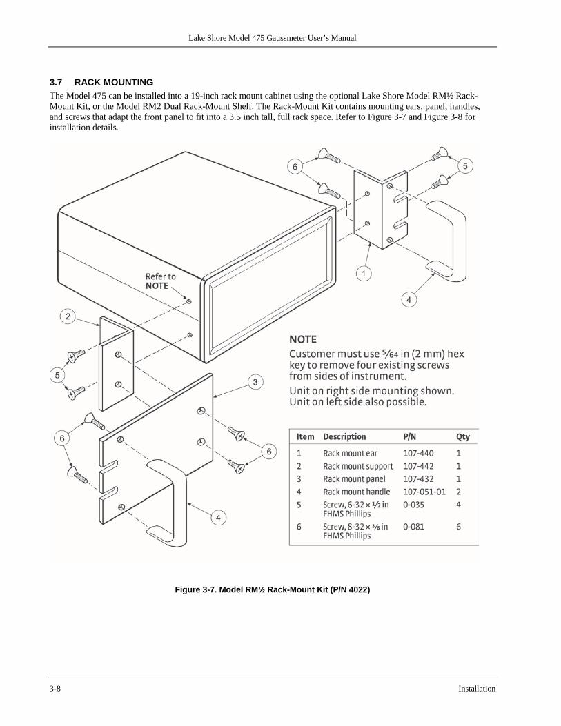
Lake Shore Model 475 Gaussmeter User’s Manual
3-8 Installation
3.7 RACK MOUNTING The Model 475 can be installed into a 19-inch rack mount cabinet using the optional Lake Shore Model RM½ Rack-Mount Kit, or the Model RM2 Dual Rack-Mount Shelf. The Rack-Mount Kit contains mounting ears, panel, handles, and screws that adapt the front panel to fit into a 3.5 inch tall, full rack space. Refer to Figure 3-7 and Figure 3-8 for installation details.
Figure 3-7. Model RM½ Rack-Mount Kit (P/N 4022)

Lake Shore Model 475 Gaussmeter User’s Manual
Installation 3-9
Figure 3-8. Model RM2 Dual Rack-Mount Shelf (P/N 4026)

Lake Shore Model 475 Gaussmeter User’s Manual
3-10 Installation
This Page Intentionally Left Blank
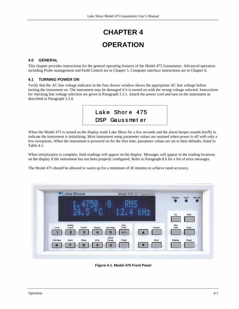
Lake Shore Model 475 Gaussmeter User’s Manual
Operation 4-1
CHAPTER 4
OPERATION
4.0 GENERAL This chapter provides instructions for the general operating features of the Model 475 Gaussmeter. Advanced operation including Probe management and Field Control are in Chapter 5. Computer interface instructions are in Chapter 6.
4.1 TURNING POWER ON Verify that the AC line voltage indicator in the fuse drawer window shows the appropriate AC line voltage before turning the instrument on. The instrument may be damaged if it is turned on with the wrong voltage selected. Instructions for checking line voltage selection are given in Paragraph 3.3.1. Attach the power cord and turn on the instrument as described in Paragraph 3.3.4.
Lak e Shor e 475 DSP Gaus s met er
When the Model 475 is turned on the display reads Lake Shore for a few seconds and the alarm beeper sounds briefly to indicate the instrument is initializing. Most instrument setup parameter values are retained when power is off with only a few exceptions. When the instrument is powered on for the first time, parameter values are set to their defaults, listed in Table 4-1. When initialization is complete, field readings will appear on the display. Messages will appear in the reading locations on the display if the instrument has not been properly configured. Refer to Paragraph 8.6 for a list of error messages. The Model 475 should be allowed to warm up for a minimum of 30 minutes to achieve rated accuracy.
Figure 4-1. Model 475 Front Panel
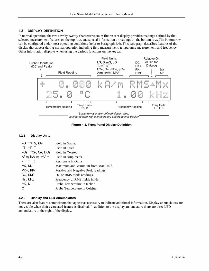
Lake Shore Model 475 Gaussmeter User’s Manual
4-2 Operation
4.2 DISPLAY DEFINITION In normal operation, the two row by twenty character vacuum fluorescent display provides readings defined by the selected measurement features on the top row, and special information or readings on the bottom row. The bottom row can be configured under most operating conditions (refer to Paragraph 4.4). This paragraph describes features of the display that appear during normal operation including field measurement, temperature measurement, and frequency. Other information displays when using the various functions on the keypad.
Figure 4-2. Front Panel Display Definition
4.2.1 Display Units
¬G, mG, G, kG Field in Gauss. ¬T, mT, T Field in Tesla ¬Oe, mOe, Oe, kOe Field in Oersted A/ m, kA/ m, MA/ m Field in Amp/meter ¬¦ , m¦ , ¦ Resistance in Ohms MX, MN Maximum and Minimum from Max Hold PK+, PK- Positive and Negative Peak readings DC, RMS DC or RMS mode readings Hz, kHz Frequency of RMS fields in Hz mK, K Probe Temperature in Kelvin C Probe Temperature in Celsius
4.2.2 Display and LED Annunciators There are also feature annunciators that appear as necessary to indicate additional information. Display annunciators are not visible when their associated feature is disabled. In addition to the display annunciators there are three LED annunciators to the right of the display.
Lake Shore Model 475 Gaussmeter User’s Manual
Operation 4-3
Display Annunciators ° Indicates that the Relative measurement mode is on. SP Indicates the Relative setpoint value. CSP Indicates the Field Control setpoint value.
LED Annunciators
Relative Indicates that the Relative measurement mode is on. Alarm On steady when the alarm feature is on, blinks when the alarm is active . Remote Indicates that the instrument is under remote control of the computer interface.
4.3 KEYPAD DEFINITION The Model 475 has 22 keys separated into 3 groups on the instrument front panel.
4.3.1 Key Descriptions
Local Returns the instrument to Local mode if in Remote (Chapter 6) Analog Output Setup Analog Output 3 Control Configure the Model 475 Field Control parameters (Chapter 5) Display Configure bottom line of display Autorange Turns Auto Range feature ON and OFF. Zero Probe Zeros or nulls effects of ambient low level fields from the probe Interface Setup computer interface parameters (Chapter 6) Alarm Turns Alarm feature ON and OFF, and setup alarm parameters Relay Setup Relay feature Units Configure units of measurement for Field and Temperature (if available) Select Range Manually selects field measurement range Probe Setup and view Probe parameters. Extension cable programming 0-9, ±, . Numeric data entry within a setting sequence s (Up) Increments a parameter selection or value in a numerical display t (Down) Decrements a parameter selection or value in a numerical display Escape Exits from parameter setting sequence without changing the parameter value. Press and hold
Escape for 6 seconds to view firmware date and for setting parameters to factory defaults. Enter Accepts changes in the parameter setting display. Press and hold Enter to access the Keypad Lock
feature. DC Select DC Field measurement. Press and hold to select Filter. RMS Select AC Root Mean Square (RMS) measurement. Press and hold for filter configuration Max Hold Turns Max Hold feature ON and OFF Peak Select Peak measurement. Press and hold for peak configuration Relative Turns Relative feature ON and OFF. Reset Reset max, min or peak readings depending on which measurement is active
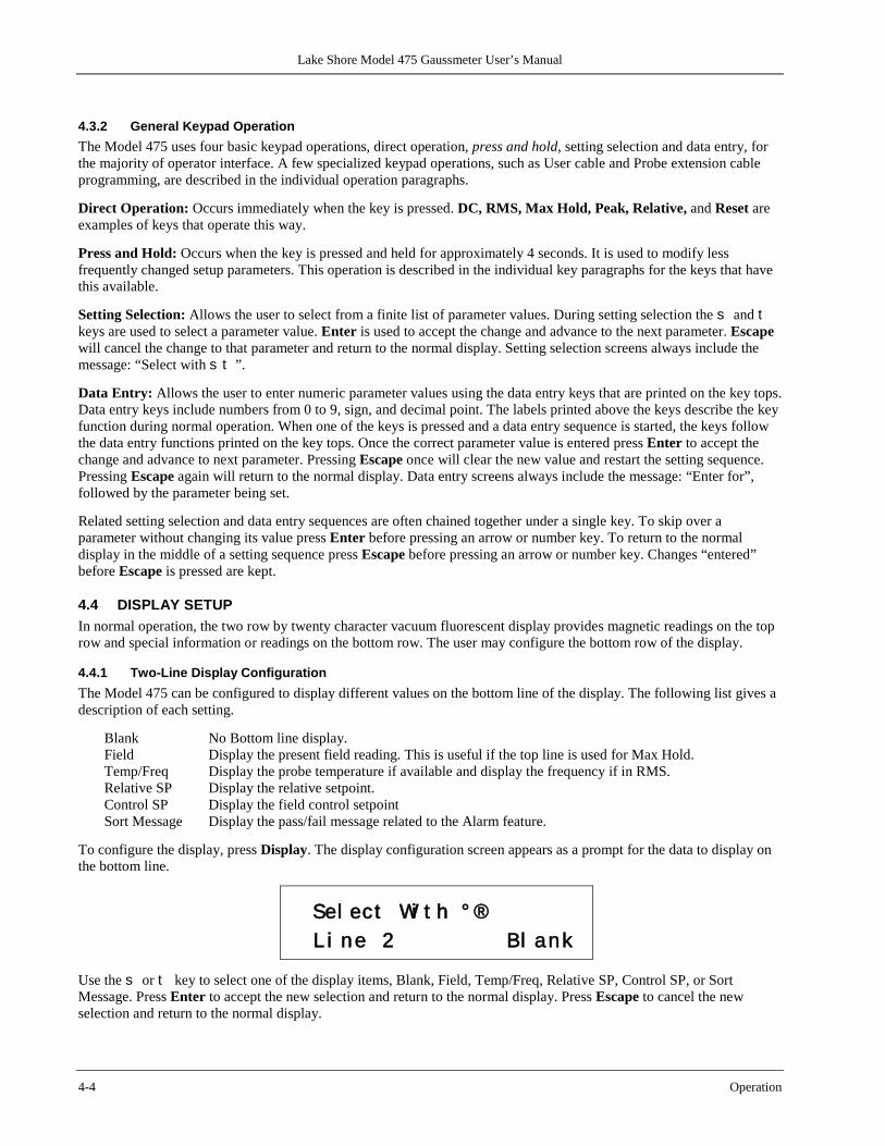
Lake Shore Model 475 Gaussmeter User’s Manual
4-4 Operation
4.3.2 General Keypad Operation The Model 475 uses four basic keypad operations, direct operation, press and hold, setting selection and data entry, for the majority of operator interface. A few specialized keypad operations, such as User cable and Probe extension cable programming, are described in the individual operation paragraphs. Direct Operation: Occurs immediately when the key is pressed. DC, RMS, Max Hold, Peak, Relative, and Reset are examples of keys that operate this way. Press and Hold: Occurs when the key is pressed and held for approximately 4 seconds. It is used to modify less frequently changed setup parameters. This operation is described in the individual key paragraphs for the keys that have this available. Setting Selection: Allows the user to select from a finite list of parameter values. During setting selection the s and t keys are used to select a parameter value. Enter is used to accept the change and advance to the next parameter. Escape will cancel the change to that parameter and return to the normal display. Setting selection screens always include the message: “Select with s t ”. Data Entry: Allows the user to enter numeric parameter values using the data entry keys that are printed on the key tops. Data entry keys include numbers from 0 to 9, sign, and decimal point. The labels printed above the keys describe the key function during normal operation. When one of the keys is pressed and a data entry sequence is started, the keys follow the data entry functions printed on the key tops. Once the correct parameter value is entered press Enter to accept the change and advance to next parameter. Pressing Escape once will clear the new value and restart the setting sequence. Pressing Escape again will return to the normal display. Data entry screens always include the message: “Enter for”, followed by the parameter being set. Related setting selection and data entry sequences are often chained together under a single key. To skip over a parameter without changing its value press Enter before pressing an arrow or number key. To return to the normal display in the middle of a setting sequence press Escape before pressing an arrow or number key. Changes “entered” before Escape is pressed are kept.
4.4 DISPLAY SETUP In normal operation, the two row by twenty character vacuum fluorescent display provides magnetic readings on the top row and special information or readings on the bottom row. The user may configure the bottom row of the display.
4.4.1 Two-Line Display Configuration The Model 475 can be configured to display different values on the bottom line of the display. The following list gives a description of each setting.
Blank No Bottom line display. Field Display the present field reading. This is useful if the top line is used for Max Hold. Temp/Freq Display the probe temperature if available and display the frequency if in RMS. Relative SP Display the relative setpoint. Control SP Display the field control setpoint Sort Message Display the pass/fail message related to the Alarm feature.
To configure the display, press Display. The display configuration screen appears as a prompt for the data to display on the bottom line.
Sel ect Wi t h ° ® L i ne 2 Bl ank
Use the s or t key to select one of the display items, Blank, Field, Temp/Freq, Relative SP, Control SP, or Sort Message. Press Enter to accept the new selection and return to the normal display. Press Escape to cancel the new selection and return to the normal display.
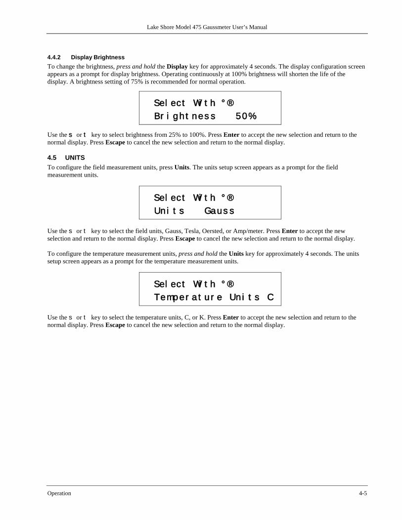
Lake Shore Model 475 Gaussmeter User’s Manual
Operation 4-5
4.4.2 Display Brightness To change the brightness, press and hold the Display key for approximately 4 seconds. The display configuration screen appears as a prompt for display brightness. Operating continuously at 100% brightness will shorten the life of the display. A brightness setting of 75% is recommended for normal operation.
Sel ect Wi t h ° ® Br i gh t nes s 50%
Use the s or t key to select brightness from 25% to 100%. Press Enter to accept the new selection and return to the normal display. Press Escape to cancel the new selection and return to the normal display.
4.5 UNITS To configure the field measurement units, press Units. The units setup screen appears as a prompt for the field measurement units.
Sel ect Wi t h ° ® Un i t s Gaus s
Use the s or t key to select the field units, Gauss, Tesla, Oersted, or Amp/meter. Press Enter to accept the new selection and return to the normal display. Press Escape to cancel the new selection and return to the normal display. To configure the temperature measurement units, press and hold the Units key for approximately 4 seconds. The units setup screen appears as a prompt for the temperature measurement units.
Sel ect Wi t h ° ® Temper a t u r e Un i t s C
Use the s or t key to select the temperature units, C, or K. Press Enter to accept the new selection and return to the normal display. Press Escape to cancel the new selection and return to the normal display.
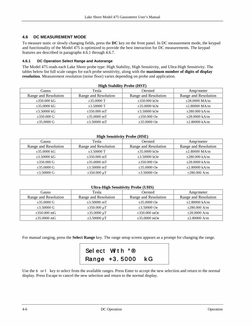
Lake Shore Model 475 Gaussmeter User’s Manual
4-6 DC Operation Operation
4.6 DC MEASUREMENT MODE To measure static or slowly changing fields, press the DC key on the front panel. In DC measurement mode, the keypad and functionality of the Model 475 is optimized to provide the best interaction for DC measurements. The keypad features are described in paragraphs 4.6.1 through 4.6.7.
4.6.1 DC Operation Select Range and Autorange The Model 475 reads each Lake Shore probe type: High Stability, High Sensitivity, and Ultra-High Sensitivity. The tables below list full scale ranges for each probe sensitivity, along with the maximum number of digits of display resolution. Measurement resolution (noise floor) varies depending on probe and application.
High Stability Probe (HST) Gauss Tesla Oersted Amp/meter
Range and Resolution Range and Resolution Range and Resolution Range and Resolution ±350.000 kG ±35.0000 T ±350.000 kOe ±28.0000 MA/m
±35.0000 kG ±3.50000 T ±35.0000 kOe ±2.80000 MA/m
±3.50000 kG ±350.000 mT ±3.50000 kOe ±280.000 kA/m ±350.000 G ±35.0000 mT ±350.000 Oe ±28.0000 kA/m ±35.0000 G ±3.50000 mT ±35.0000 Oe ±2.80000 kA/m
High Sensitivity Probe (HSE) Gauss Tesla Oersted Amp/meter
Range and Resolution Range and Resolution Range and Resolution Range and Resolution ±35.0000 kG ±3.50000 T ±35.0000 kOe ±2.80000 MA/m
±3.50000 kG ±350.000 mT ±3.50000 kOe ±280.000 kA/m ±350.000 G ±35.0000 mT ±350.000 Oe ±28.0000 kA/m ±35.0000 G ±3.50000 mT ±35.0000 Oe ±2.80000 kA/m ±3.50000 G ±350.000 µT ±3.50000 Oe ±280.000 A/m
Ultra-High Sensitivity Probe (UHS) Gauss Tesla Oersted Amp/meter
Range and Resolution Range and Resolution Range and Resolution Range and Resolution ±35.0000 G ±3.50000 mT ±35.0000 Oe ±2.80000 kA/m
±3.50000 G ±350.000 µT ±3.50000 Oe ±280.000 A/m ±350.000 mG ±35.0000 µT ±350.000 mOe ±28.0000 A/m ±35.0000 mG ±3.50000 µT ±35.0000 mOe ±2.80000 A/m
For manual ranging, press the Select Range key. The range setup screen appears as a prompt for changing the range.
Sel ect Wi t h ° ® Range +3 . 5000 k G
Use the s or t key to select from the available ranges. Press Enter to accept the new selection and return to the normal display. Press Escape to cancel the new selection and return to the normal display.
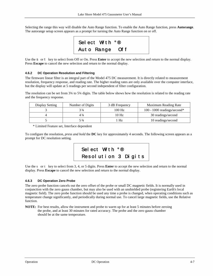
Lake Shore Model 475 Gaussmeter User’s Manual
Operation DC Operation 4-7
Selecting the range this way will disable the Auto Range function. To enable the Auto Range function, press Autorange. The autorange setup screen appears as a prompt for turning the Auto Range function on or off.
Sel ect Wi t h ° ® Au t o Range Of f
Use the s or t key to select from Off or On. Press Enter to accept the new selection and return to the normal display. Press Escape to cancel the new selection and return to the normal display.
4.6.2 DC Operation Resolution and Filtering The firmware linear filter is an integral part of the Model 475 DC measurement. It is directly related to measurement resolution, frequency response, and reading rate. The higher reading rates are only available over the computer interface, but the display will update at 5 readings per second independent of filter configuration. The resolution can be set from 3¾ to 5¾ digits. The table below shows how the resolution is related to the reading rate and the frequency response.
Display Setting Number of Digits 3 dB Frequency Maximum Reading Rate 3 3 ¾ 100 Hz 100 – 1000 readings/second* 4 4 ¾ 10 Hz 30 readings/second 5 5 ¾ 1 Hz 10 readings/second
* Limited Feature set, Interface dependent To configure the resolution, press and hold the DC key for approximately 4 seconds. The following screen appears as a prompt for DC resolution setting.
Sel ect Wi t h ° ® Res o l u t i on 3 Di g i t s
Use the s or t key to select from 3, 4, or 5 digits. Press Enter to accept the new selection and return to the normal display. Press Escape to cancel the new selection and return to the normal display.
4.6.3 DC Operation Zero Probe The zero probe function cancels out the zero offset of the probe or small DC magnetic fields. It is normally used in conjunction with the zero gauss chamber, but may also be used with an unshielded probe (registering Earth's local magnetic field). The zero probe function should be used any time a probe is changed, when operating conditions such as temperature change significantly, and periodically during normal use. To cancel large magnetic fields, use the Relative function.
NOTE: For best results, allow the instrument and probe to warm up for at least 5 minutes before zeroing the probe, and at least 30 minutes for rated accuracy. The probe and the zero gauss chamber should be at the same temperature.
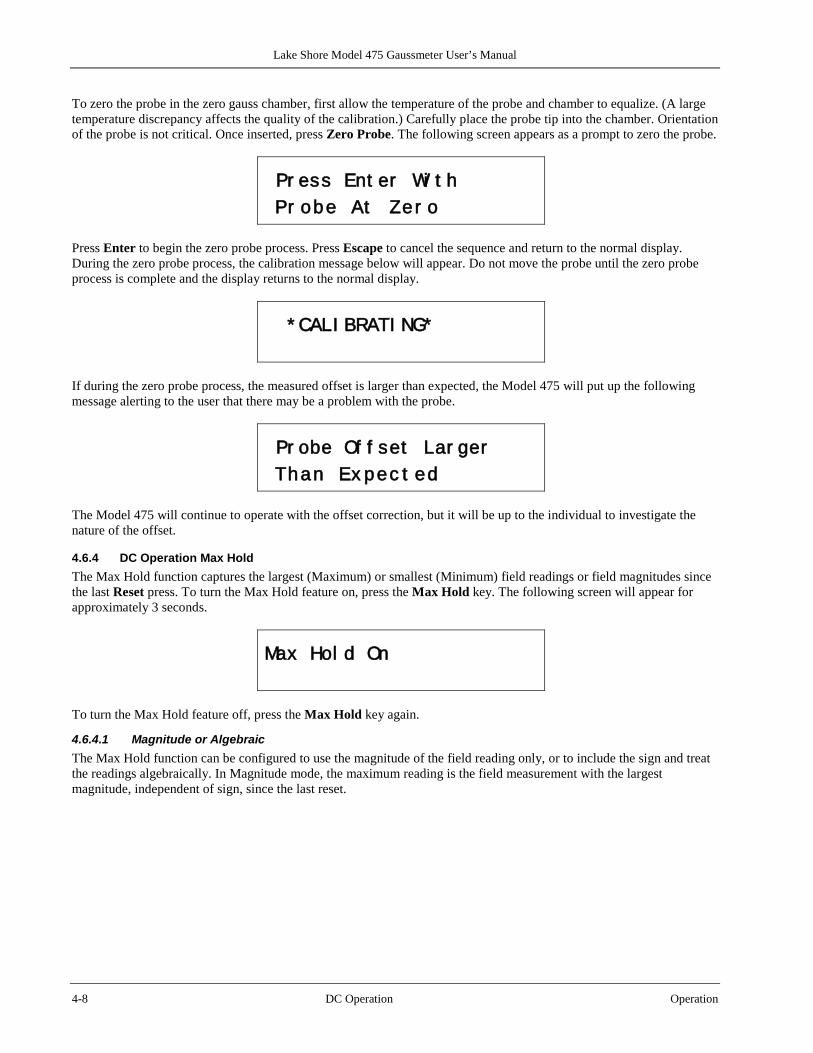
Lake Shore Model 475 Gaussmeter User’s Manual
4-8 DC Operation Operation
To zero the probe in the zero gauss chamber, first allow the temperature of the probe and chamber to equalize. (A large temperature discrepancy affects the quality of the calibration.) Carefully place the probe tip into the chamber. Orientation of the probe is not critical. Once inserted, press Zero Probe. The following screen appears as a prompt to zero the probe.
Pr ess Ent er Wi t h Pr obe At Zer o
Press Enter to begin the zero probe process. Press Escape to cancel the sequence and return to the normal display. During the zero probe process, the calibration message below will appear. Do not move the probe until the zero probe process is complete and the display returns to the normal display.
* CALI BRATI NG*
If during the zero probe process, the measured offset is larger than expected, the Model 475 will put up the following message alerting to the user that there may be a problem with the probe.
Pr obe Of f set Lar ger Than Ex pec t ed
The Model 475 will continue to operate with the offset correction, but it will be up to the individual to investigate the nature of the offset.
4.6.4 DC Operation Max Hold The Max Hold function captures the largest (Maximum) or smallest (Minimum) field readings or field magnitudes since the last Reset press. To turn the Max Hold feature on, press the Max Hold key. The following screen will appear for approximately 3 seconds.
Max Hol d On
To turn the Max Hold feature off, press the Max Hold key again.
4.6.4.1 Magnitude or Algebraic The Max Hold function can be configured to use the magnitude of the field reading only, or to include the sign and treat the readings algebraically. In Magnitude mode, the maximum reading is the field measurement with the largest magnitude, independent of sign, since the last reset.
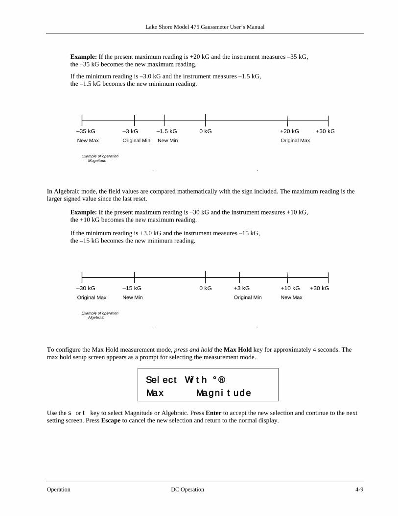
Lake Shore Model 475 Gaussmeter User’s Manual
Operation DC Operation 4-9
Example: If the present maximum reading is +20 kG and the instrument measures –35 kG, the –35 kG becomes the new maximum reading.
If the minimum reading is –3.0 kG and the instrument measures –1.5 kG, the –1.5 kG becomes the new minimum reading.
0 kG +20 kG +30 kG –35 kG –3 kG –1.5 kG Original Max
Example of operation Magnitude
New Max Original Min New Min
In Algebraic mode, the field values are compared mathematically with the sign included. The maximum reading is the larger signed value since the last reset.
Example: If the present maximum reading is –30 kG and the instrument measures +10 kG, the +10 kG becomes the new maximum reading. If the minimum reading is +3.0 kG and the instrument measures –15 kG, the –15 kG becomes the new minimum reading.
0 kG +3 kG +10 kG –30 kG –15 kG +30 kG New Max
Example of operation Algebraic
Original Max New Min Original Min
To configure the Max Hold measurement mode, press and hold the Max Hold key for approximately 4 seconds. The max hold setup screen appears as a prompt for selecting the measurement mode.
Sel ect Wi t h ° ® Max Magn i t ude
Use the s or t key to select Magnitude or Algebraic. Press Enter to accept the new selection and continue to the next setting screen. Press Escape to cancel the new selection and return to the normal display.
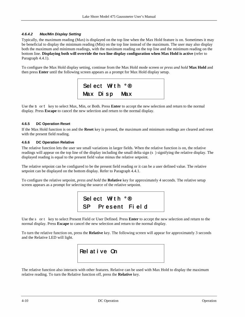
Lake Shore Model 475 Gaussmeter User’s Manual
4-10 DC Operation Operation
4.6.4.2 Max/Min Display Setting Typically, the maximum reading (Max) is displayed on the top line when the Max Hold feature is on. Sometimes it may be beneficial to display the minimum reading (Min) on the top line instead of the maximum. The user may also display both the maximum and minimum readings, with the maximum reading on the top line and the minimum reading on the bottom line. Displaying both will override the two line display configuration when Max Hold is active (refer to Paragraph 4.4.1). To configure the Max Hold display setting, continue from the Max Hold mode screen or press and hold Max Hold and then press Enter until the following screen appears as a prompt for Max Hold display setup.
Sel ect Wi t h ° ® Max Di s p Max
Use the s or t key to select Max, Min, or Both. Press Enter to accept the new selection and return to the normal display. Press Escape to cancel the new selection and return to the normal display.
4.6.5 DC Operation Reset If the Max Hold function is on and the Reset key is pressed, the maximum and minimum readings are cleared and reset with the present field reading.
4.6.6 DC Operation Relative The relative function lets the user see small variations in larger fields. When the relative function is on, the relative readings will appear on the top line of the display including the small delta sign (s ) signifying the relative display. The displayed reading is equal to the present field value minus the relative setpoint. The relative setpoint can be configured to be the present field reading or it can be a user defined value. The relative setpoint can be displayed on the bottom display. Refer to Paragraph 4.4.1. To configure the relative setpoint, press and hold the Relative key for approximately 4 seconds. The relative setup screen appears as a prompt for selecting the source of the relative setpoint.
Sel ect Wi t h ° ® SP Pr es en t Fi e l d
Use the s or t key to select Present Field or User Defined. Press Enter to accept the new selection and return to the normal display. Press Escape to cancel the new selection and return to the normal display. To turn the relative function on, press the Relative key. The following screen will appear for approximately 3 seconds and the Relative LED will light.
Rel at i ve On
The relative function also interacts with other features. Relative can be used with Max Hold to display the maximum relative reading. To turn the Relative function off, press the Relative key.
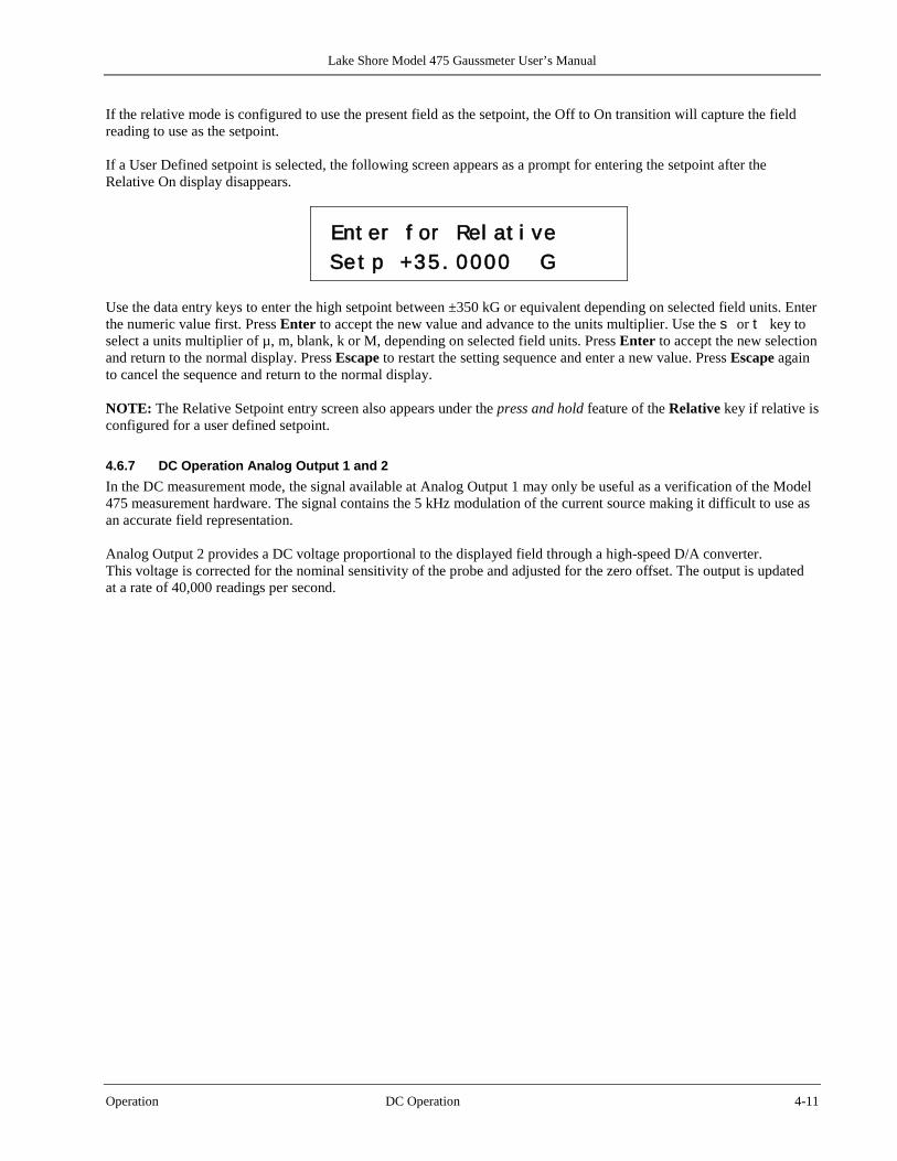
Lake Shore Model 475 Gaussmeter User’s Manual
Operation DC Operation 4-11
If the relative mode is configured to use the present field as the setpoint, the Off to On transition will capture the field reading to use as the setpoint. If a User Defined setpoint is selected, the following screen appears as a prompt for entering the setpoint after the Relative On display disappears.
Ent er f or Rel at i ve Se t p +35 . 0000 G
Use the data entry keys to enter the high setpoint between ±350 kG or equivalent depending on selected field units. Enter the numeric value first. Press Enter to accept the new value and advance to the units multiplier. Use the s or t key to select a units multiplier of µ, m, blank, k or M, depending on selected field units. Press Enter to accept the new selection and return to the normal display. Press Escape to restart the setting sequence and enter a new value. Press Escape again to cancel the sequence and return to the normal display. NOTE: The Relative Setpoint entry screen also appears under the press and hold feature of the Relative key if relative is configured for a user defined setpoint.
4.6.7 DC Operation Analog Output 1 and 2 In the DC measurement mode, the signal available at Analog Output 1 may only be useful as a verification of the Model 475 measurement hardware. The signal contains the 5 kHz modulation of the current source making it difficult to use as an accurate field representation. Analog Output 2 provides a DC voltage proportional to the displayed field through a high-speed D/A converter. This voltage is corrected for the nominal sensitivity of the probe and adjusted for the zero offset. The output is updated at a rate of 40,000 readings per second.
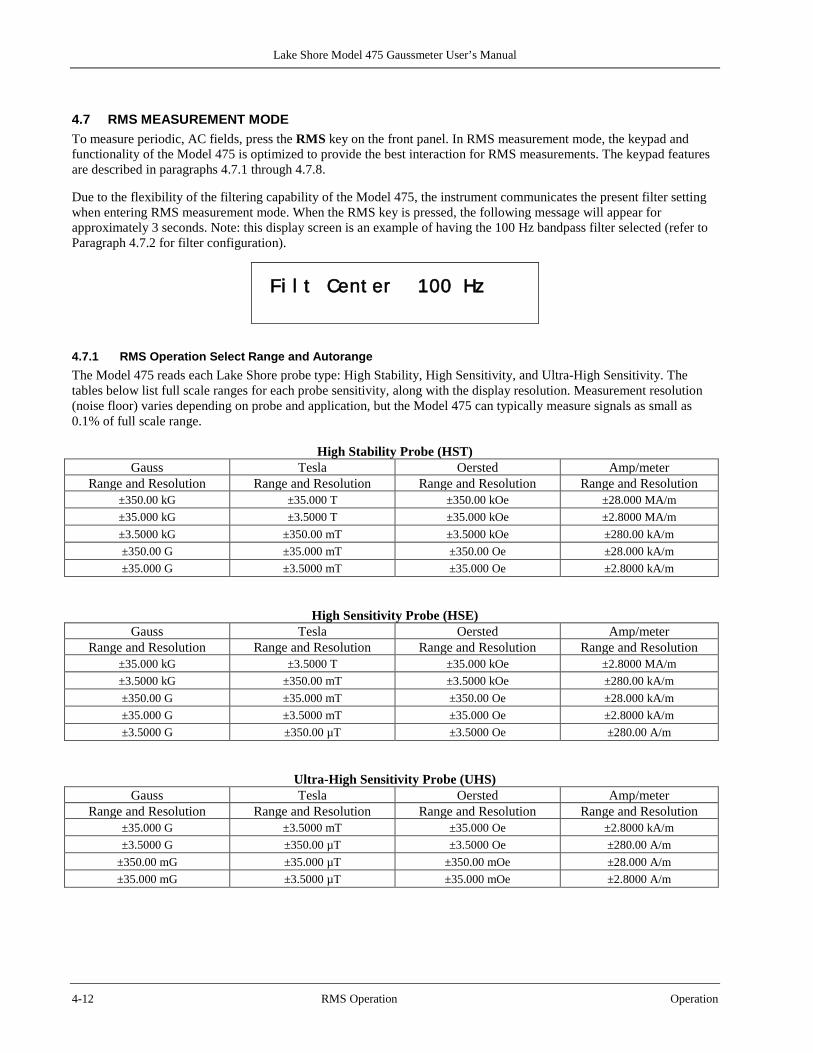
Lake Shore Model 475 Gaussmeter User’s Manual
4-12 RMS Operation Operation
4.7 RMS MEASUREMENT MODE To measure periodic, AC fields, press the RMS key on the front panel. In RMS measurement mode, the keypad and functionality of the Model 475 is optimized to provide the best interaction for RMS measurements. The keypad features are described in paragraphs 4.7.1 through 4.7.8. Due to the flexibility of the filtering capability of the Model 475, the instrument communicates the present filter setting when entering RMS measurement mode. When the RMS key is pressed, the following message will appear for approximately 3 seconds. Note: this display screen is an example of having the 100 Hz bandpass filter selected (refer to Paragraph 4.7.2 for filter configuration).
Fi l t Cent er 100 Hz
4.7.1 RMS Operation Select Range and Autorange The Model 475 reads each Lake Shore probe type: High Stability, High Sensitivity, and Ultra-High Sensitivity. The tables below list full scale ranges for each probe sensitivity, along with the display resolution. Measurement resolution (noise floor) varies depending on probe and application, but the Model 475 can typically measure signals as small as 0.1% of full scale range.
High Stability Probe (HST) Gauss Tesla Oersted Amp/meter
Range and Resolution Range and Resolution Range and Resolution Range and Resolution ±350.00 kG ±35.000 T ±350.00 kOe ±28.000 MA/m
±35.000 kG ±3.5000 T ±35.000 kOe ±2.8000 MA/m
±3.5000 kG ±350.00 mT ±3.5000 kOe ±280.00 kA/m ±350.00 G ±35.000 mT ±350.00 Oe ±28.000 kA/m ±35.000 G ±3.5000 mT ±35.000 Oe ±2.8000 kA/m
High Sensitivity Probe (HSE) Gauss Tesla Oersted Amp/meter
Range and Resolution Range and Resolution Range and Resolution Range and Resolution ±35.000 kG ±3.5000 T ±35.000 kOe ±2.8000 MA/m
±3.5000 kG ±350.00 mT ±3.5000 kOe ±280.00 kA/m ±350.00 G ±35.000 mT ±350.00 Oe ±28.000 kA/m ±35.000 G ±3.5000 mT ±35.000 Oe ±2.8000 kA/m ±3.5000 G ±350.00 µT ±3.5000 Oe ±280.00 A/m
Ultra-High Sensitivity Probe (UHS) Gauss Tesla Oersted Amp/meter
Range and Resolution Range and Resolution Range and Resolution Range and Resolution ±35.000 G ±3.5000 mT ±35.000 Oe ±2.8000 kA/m
±3.5000 G ±350.00 µT ±3.5000 Oe ±280.00 A/m ±350.00 mG ±35.000 µT ±350.00 mOe ±28.000 A/m ±35.000 mG ±3.5000 µT ±35.000 mOe ±2.8000 A/m
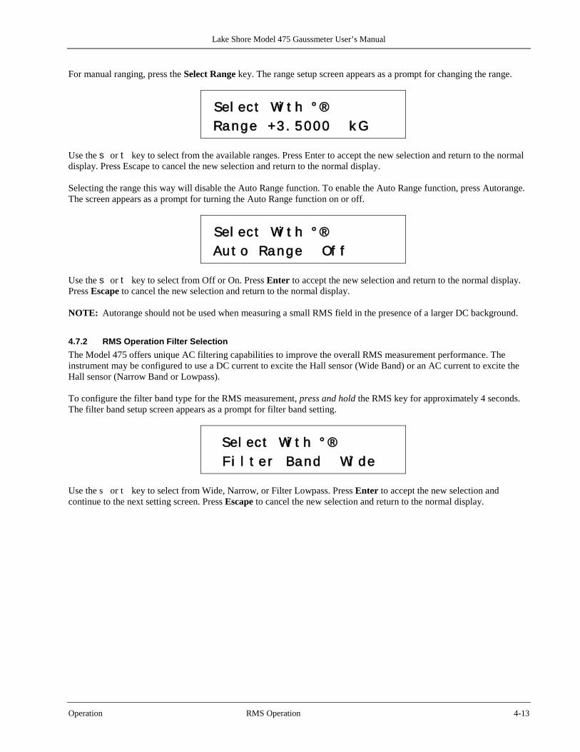
Lake Shore Model 475 Gaussmeter User’s Manual
Operation RMS Operation 4-13
For manual ranging, press the Select Range key. The range setup screen appears as a prompt for changing the range.
Sel ect Wi t h ° ® Range +3 . 5000 k G
Use the s or t key to select from the available ranges. Press Enter to accept the new selection and return to the normal display. Press Escape to cancel the new selection and return to the normal display. Selecting the range this way will disable the Auto Range function. To enable the Auto Range function, press Autorange. The screen appears as a prompt for turning the Auto Range function on or off.
Sel ect Wi t h ° ® Au t o Range Of f
Use the s or t key to select from Off or On. Press Enter to accept the new selection and return to the normal display. Press Escape to cancel the new selection and return to the normal display. NOTE: Autorange should not be used when measuring a small RMS field in the presence of a larger DC background.
4.7.2 RMS Operation Filter Selection The Model 475 offers unique AC filtering capabilities to improve the overall RMS measurement performance. The instrument may be configured to use a DC current to excite the Hall sensor (Wide Band) or an AC current to excite the Hall sensor (Narrow Band or Lowpass). To configure the filter band type for the RMS measurement, press and hold the RMS key for approximately 4 seconds. The filter band setup screen appears as a prompt for filter band setting.
Sel ect Wi t h ° ® Fi l t e r Band Wi de
Use the s or t key to select from Wide, Narrow, or Filter Lowpass. Press Enter to accept the new selection and continue to the next setting screen. Press Escape to cancel the new selection and return to the normal display.
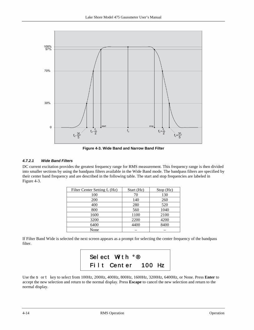
Lake Shore Model 475 Gaussmeter User’s Manual
4-14 RMS Operation Operation
Figure 4-3. Wide Band and Narrow Band Filter
4.7.2.1 Wide Band Filters DC current excitation provides the greatest frequency range for RMS measurement. This frequency range is then divided into smaller sections by using the bandpass filters available in the Wide Band mode. The bandpass filters are specified by their center band frequency and are described in the following table. The start and stop frequencies are labeled in Figure 4-3.
Filter Center Setting fc (Hz) Start (Hz) Stop (Hz) 100 70 130 200 140 260 400 280 520 800 560 1040
1600 1100 2100 3200 2200 4200 6400 4400 8400 None – –
If Filter Band Wide is selected the next screen appears as a prompt for selecting the center frequency of the bandpass filter.
Sel ect Wi t h ° ® Fi l t Cent er 100 Hz
Use the s or t key to select from 100Hz, 200Hz, 400Hz, 800Hz, 1600Hz, 3200Hz, 6400Hz, or None. Press Enter to accept the new selection and return to the normal display. Press Escape to cancel the new selection and return to the normal display.
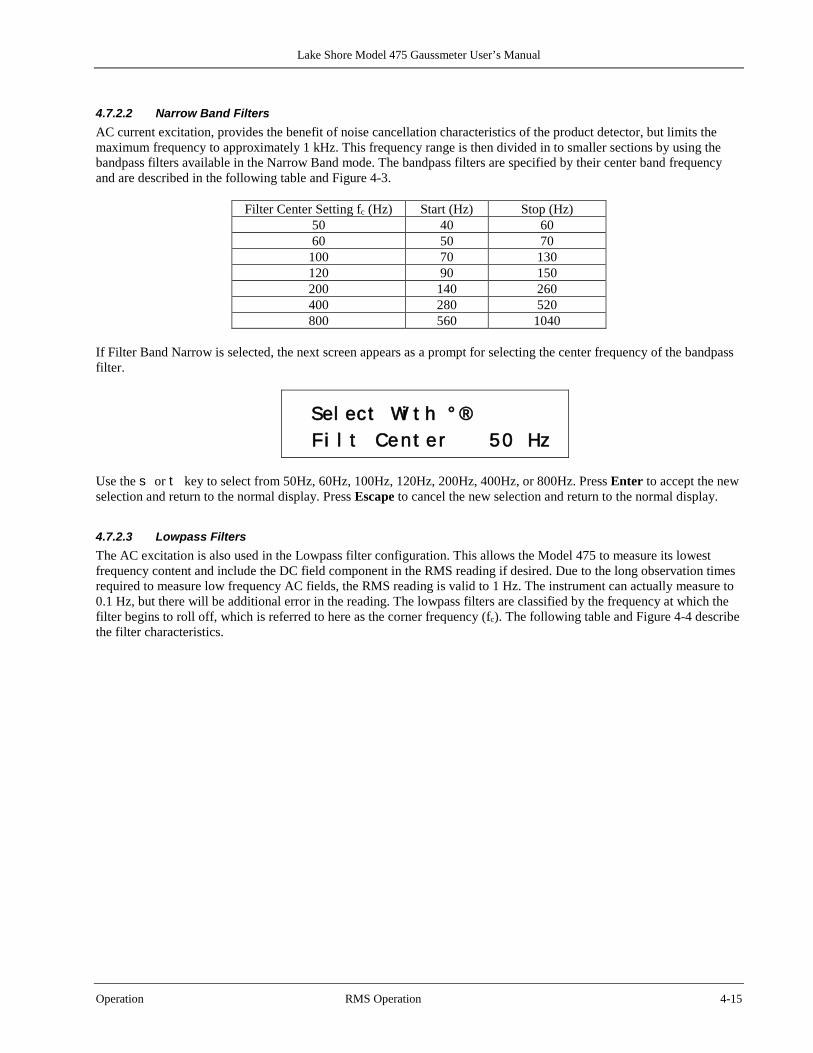
Lake Shore Model 475 Gaussmeter User’s Manual
Operation RMS Operation 4-15
4.7.2.2 Narrow Band Filters AC current excitation, provides the benefit of noise cancellation characteristics of the product detector, but limits the maximum frequency to approximately 1 kHz. This frequency range is then divided in to smaller sections by using the bandpass filters available in the Narrow Band mode. The bandpass filters are specified by their center band frequency and are described in the following table and Figure 4-3.
Filter Center Setting fc (Hz) Start (Hz) Stop (Hz) 50 40 60 60 50 70
100 70 130 120 90 150 200 140 260 400 280 520 800 560 1040
If Filter Band Narrow is selected, the next screen appears as a prompt for selecting the center frequency of the bandpass filter.
Sel ect Wi t h ° ® Fi l t Cent er 50 Hz
Use the s or t key to select from 50Hz, 60Hz, 100Hz, 120Hz, 200Hz, 400Hz, or 800Hz. Press Enter to accept the new selection and return to the normal display. Press Escape to cancel the new selection and return to the normal display.
4.7.2.3 Lowpass Filters The AC excitation is also used in the Lowpass filter configuration. This allows the Model 475 to measure its lowest frequency content and include the DC field component in the RMS reading if desired. Due to the long observation times required to measure low frequency AC fields, the RMS reading is valid to 1 Hz. The instrument can actually measure to 0.1 Hz, but there will be additional error in the reading. The lowpass filters are classified by the frequency at which the filter begins to roll off, which is referred to here as the corner frequency (fc). The following table and Figure 4-4 describe the filter characteristics.
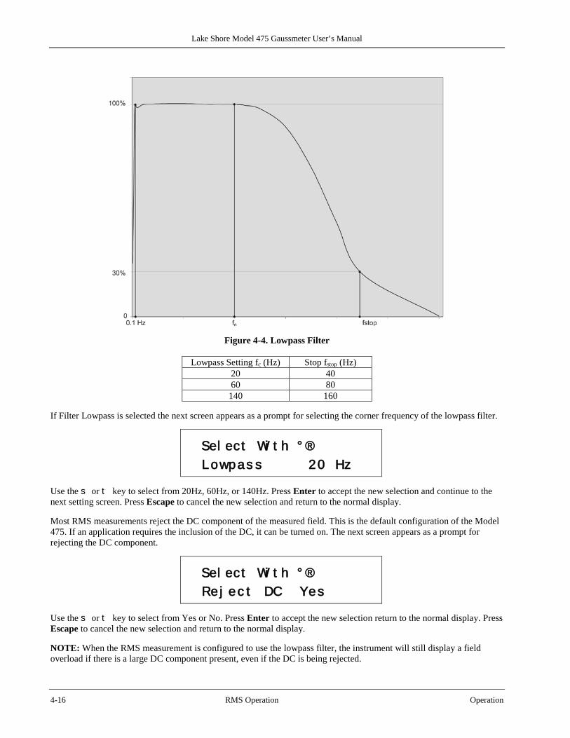
Lake Shore Model 475 Gaussmeter User’s Manual
4-16 RMS Operation Operation
Figure 4-4. Lowpass Filter
Lowpass Setting fc (Hz) Stop fstop (Hz) 20 40 60 80
140 160 If Filter Lowpass is selected the next screen appears as a prompt for selecting the corner frequency of the lowpass filter.
Sel ect Wi t h ° ® Lowpas s 20 Hz
Use the s or t key to select from 20Hz, 60Hz, or 140Hz. Press Enter to accept the new selection and continue to the next setting screen. Press Escape to cancel the new selection and return to the normal display. Most RMS measurements reject the DC component of the measured field. This is the default configuration of the Model 475. If an application requires the inclusion of the DC, it can be turned on. The next screen appears as a prompt for rejecting the DC component.
Sel ect Wi t h ° ® Re j ec t DC Yes
Use the s or t key to select from Yes or No. Press Enter to accept the new selection return to the normal display. Press Escape to cancel the new selection and return to the normal display. NOTE: When the RMS measurement is configured to use the lowpass filter, the instrument will still display a field overload if there is a large DC component present, even if the DC is being rejected.

Lake Shore Model 475 Gaussmeter User’s Manual
Operation RMS Operation 4-17
4.7.3 RMS Operation Frequency Measurement With certain limitations, the Model 475 Gaussmeter is capable of measuring and displaying the frequency of an AC magnetic field. The frequency is calculated using a zero-crossing counter, so the indicated value is only valid for robust fields with a single, dominant frequency. Because of sampling rate limitations, the reading is correct only up to 20 kHz. Refer to Paragraph 4.4.1 to configure the display to indicate frequency.
4.7.4 RMS Operation Reading Rate In RMS measurement mode, the reading update rate is dependant on the filter chosen. Longer observation times are necessary to properly measure lower frequency signals. The table below shows the reading update rate for each of the filter settings. The display will update at 5 readings per second independent of the filter setting except for the lowpass filters which update once every 2 seconds.
Filter Type Filter Frequency Reading Rate Wide Band None 312.5 readings/second * Wide Band 6400 Hz 312.5 readings/second * Wide Band 3200 Hz 156.3 readings/second * Wide Band 1600 Hz 78.1 readings/second * Wide Band 800 Hz 39.0 readings/second * Wide Band 400 Hz 19.5 readings/second Wide Band 200 Hz 9.8 readings/second Wide Band 100 Hz 4.9 readings/second
Narrow Band 800 Hz 39.0 readings/second * Narrow Band 400 Hz 19.5 readings/second Narrow Band 200 Hz 9.8 readings/second Narrow Band 120 Hz 4.9 readings/second Narrow Band 100 Hz 4.9 readings/second Narrow Band 60 Hz 4.9 readings/second Narrow Band 50 Hz 4.9 readings/second
Lowpass 140 Hz 0.6 readings/second Lowpass 60 Hz 0.6 readings/second Lowpass 20 Hz 0.6 readings/second
* Limited Feature set, Interface dependent
Lake Shore Model 475 Gaussmeter User’s Manual
4-18 RMS Operation Operation
4.7.5 RMS Operation Max Hold The Max Hold function captures the largest (Maximum) or smallest (Minimum) RMS field readings since the last Reset press. To turn the Max Hold feature on, press the Max Hold key. The following screen will appear for approximately 3 seconds.
Max Hol d On
To turn the Max Hold feature off, press the Max Hold key again.
4.7.5.1 Max/Min Display Setting Typically, the maximum reading (Max) is displayed on the top line when the Max Hold feature is on. Sometimes it may be beneficial to display the minimum reading (Min) on the top line instead of the maximum. The user may also display both the maximum and minimum readings, with the maximum reading on the top line and the minimum reading on the bottom line. Displaying both will override the two line display configuration when Max Hold is active (refer to Paragraph 4.4.1). To configure the Max Hold display setting, continue from the Max Hold mode screen or press and hold Max Hold and then press Enter until the following screen appears as a prompt for Max Hold display setup.
Sel ect Wi t h ° ® Max Di s p Max
Use the s or t key to select Max, Min, or Both. Press Enter to accept the new selection and return to the normal display. Press Escape to cancel the new selection and return to the normal display.
4.7.6 RMS Operation Reset If the Max Hold function is on and the Reset key is pressed, the maximum and minimum readings are cleared and reset with the present field reading.
4.7.7 RMS Operation Relative The relative function lets the user see small variations in larger fields. When the relative function is on, the relative readings will appear on the top line of the display including the small delta sign (s ) signifying the relative display. The displayed reading is equal to the present field value minus the relative setpoint. The relative setpoint can be configured to be the present field reading or it can be a user defined value. The relative setpoint can be displayed on the bottom display. Refer to Paragraph 4.4.1. To configure the relative setpoint, press and hold the Relative key for approximately 4 seconds. The relative setup screen appears as a prompt for selecting the source of the relative setpoint.
Sel ect Wi t h ° ® SP Pr es en t Fi e l d
Use the s or t key to select Present Field or User Defined. Press Enter to accept the new selection and return to the normal display. Press Escape to cancel the new selection and return to the normal display.
Lake Shore Model 475 Gaussmeter User’s Manual
Operation RMS Operation 4-19
To turn the relative function on, press the Relative key. The following screen will appear for approximately 3 seconds and the Relative LED will light.
Rel at i ve On
The relative function also interacts with other features. Relative can be used with Max Hold to display the maximum relative reading. To turn the Relative function off, press the Relative key. If the relative mode is configured to use the present field as the setpoint, the Off to On transition will capture the field reading to use as the setpoint. If a User Defined setpoint is selected, the following screen appears as a prompt for entering the setpoint after the Relative On display disappears.
Ent er f or Rel at i ve Se t p +35 . 0000 G
Use the data entry keys to enter the relative setpoint between ±350 kG or equivalent depending on selected field units. Enter the numeric value first. Press Enter to accept the new value and advance to the units multiplier. Use the s or t key to select a units multiplier of µ, m, blank, k or M, depending on selected field units. Press Enter to accept the new selection and return to the normal display. Press Escape to restart the setting sequence and enter a new value. Press Escape again to cancel the sequence and return to the normal display.
4.7.8 RMS Operation Analog Output 1 and 2 If the instrument is configured in Wide Band RMS measurement mode, Analog Output 1 is a real-time analog signal proportional to the AC magnetic field and scaled to ±3.5 volts for full scale of selected range, except for the lowest range which is scaled to ±0.35 volts for full scale range. The output has a frequency range of 1 Hz to 50 kHz. If the Narrow Band or Lowpass filters are used, Analog Output 1 may only be useful as a verification of the Model 475 measurement hardware. The signal contains the 5 kHz modulation of the current source making it difficult to use as an accurate field representation. Analog Output 2 provides an AC voltage proportional to the AC magnetic field through a high-speed D/A converter. This voltage is corrected for the nominal sensitivity of the probe. The output is updated at a rate of 40,000 readings per second. The Analog Output 2 is equipped with a two-pole analog lowpass filter at 145 kHz. The individual D/A samples are still visible and the signal may be improved with the addition of external analog filters.
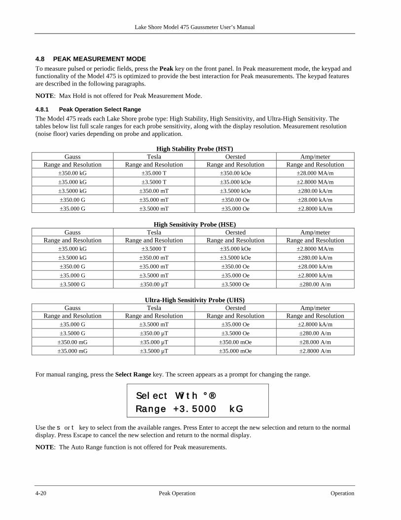
Lake Shore Model 475 Gaussmeter User’s Manual
4-20 Peak Operation Operation
4.8 PEAK MEASUREMENT MODE To measure pulsed or periodic fields, press the Peak key on the front panel. In Peak measurement mode, the keypad and functionality of the Model 475 is optimized to provide the best interaction for Peak measurements. The keypad features are described in the following paragraphs.
NOTE: Max Hold is not offered for Peak Measurement Mode.
4.8.1 Peak Operation Select Range The Model 475 reads each Lake Shore probe type: High Stability, High Sensitivity, and Ultra-High Sensitivity. The tables below list full scale ranges for each probe sensitivity, along with the display resolution. Measurement resolution (noise floor) varies depending on probe and application.
High Stability Probe (HST) Gauss Tesla Oersted Amp/meter
Range and Resolution Range and Resolution Range and Resolution Range and Resolution ±350.00 kG ±35.000 T ±350.00 kOe ±28.000 MA/m
±35.000 kG ±3.5000 T ±35.000 kOe ±2.8000 MA/m
±3.5000 kG ±350.00 mT ±3.5000 kOe ±280.00 kA/m ±350.00 G ±35.000 mT ±350.00 Oe ±28.000 kA/m ±35.000 G ±3.5000 mT ±35.000 Oe ±2.8000 kA/m
High Sensitivity Probe (HSE)
Gauss Tesla Oersted Amp/meter Range and Resolution Range and Resolution Range and Resolution Range and Resolution
±35.000 kG ±3.5000 T ±35.000 kOe ±2.8000 MA/m
±3.5000 kG ±350.00 mT ±3.5000 kOe ±280.00 kA/m ±350.00 G ±35.000 mT ±350.00 Oe ±28.000 kA/m ±35.000 G ±3.5000 mT ±35.000 Oe ±2.8000 kA/m
±3.5000 G ±350.00 µT ±3.5000 Oe ±280.00 A/m
Ultra-High Sensitivity Probe (UHS) Gauss Tesla Oersted Amp/meter
Range and Resolution Range and Resolution Range and Resolution Range and Resolution ±35.000 G ±3.5000 mT ±35.000 Oe ±2.8000 kA/m
±3.5000 G ±350.00 µT ±3.5000 Oe ±280.00 A/m ±350.00 mG ±35.000 µT ±350.00 mOe ±28.000 A/m ±35.000 mG ±3.5000 µT ±35.000 mOe ±2.8000 A/m
For manual ranging, press the Select Range key. The screen appears as a prompt for changing the range.
Sel ect Wi t h ° ® Range +3 . 5000 k G
Use the s or t key to select from the available ranges. Press Enter to accept the new selection and return to the normal display. Press Escape to cancel the new selection and return to the normal display.
NOTE: The Auto Range function is not offered for Peak measurements.

Lake Shore Model 475 Gaussmeter User’s Manual
Operation Peak Operation 4-21
4.8.2 Peak Operation Periodic/Pulse Setup The Peak measurement mode can be configured to measure pulsed fields or the maximum amplitude of periodic fields. In periodic mode, the instrument follows the peak amplitude of the periodic signal. This may be useful in determining additional information about AC fields, such as crest factor. Pulsed fields with a minimum pulse width of 20 µs can be captured using the pulse measurement mode. Once captured, these readings will only change if a larger peak is measured, or if the Reset key is pressed. To setup the periodic or pulse feature, press and hold the Peak key for approximately 4 seconds. The Peak configuration screen appears as a prompt for selecting Periodic or Pulse measurements.
Sel ect Wi t h ° ® Peak Per i od i c
Use the s or t key to select from Periodic or Pulse. Press Enter to accept the new selection and continue to the next setting screen. Press Escape to cancel the new selection and return to the normal display.
4.8.3 Peak Operation Display Setting Typically the positive peak reading (PK+) is displayed on the top line when in Peak measurement mode. Sometimes it may be beneficial to display the negative peak reading (PK–) on the top line instead of the maximum. The user may also display both peak readings, with the positive reading on the top line and the negative reading on the bottom line. Displaying both will override the two line display configuration when Peak is active (refer to Paragraph 4.4.1). To configure the Peak display setting, continue from the Periodic/Pulse selection screen or press and hold Peak and then press Enter until the following screen appears as a prompt for Peak display setup.
Sel ect Wi t h ° ® Peak Di s p PK+
Use the s or t key to select PK+, PK-, or Both. Press Enter to accept the new selection and return to the normal display. Press Escape to cancel the new selection and return to the normal display.
4.8.4 Peak Operation Reset In Peak Measurement mode, the Reset key is used to clear any captured pulsed readings.
4.8.5 Peak Operation Frequency Measurement In Peak measurement, the frequency is only measurable in Periodic mode. The frequency is calculated using a zero-crossing counter. The frequency measurement is only valid for robust fields with a single, dominant frequency. Refer to Paragraph 4.4.1 to configure the display for frequency.
Lake Shore Model 475 Gaussmeter User’s Manual
4-22 Peak Operation Operation
4.8.6 Peak Operation Relative The relative function lets the user see small variations in larger fields. When the relative function is on, the relative readings will appear on the top line of the display including the small delta sign (s ) signifying the relative display. The displayed reading is equal to the present field value minus the relative setpoint.
The relative setpoint can be configured to be the present field reading or it can be a user defined value. The relative setpoint can be displayed on the bottom display. Refer to Paragraph 4.4.1.
To configure the relative setpoint, press and hold the Relative key for approximately 4 seconds. The relative setup screen appears as a prompt for selecting the source of the relative setpoint.
Sel ect Wi t h ° ® SP Pr es en t Fi e l d
Use the s or t key to select Present Field or User Defined. Press Enter to accept the new selection and return to the normal display. Press Escape to cancel the new selection and return to the normal display.
To turn the relative function on, press the Relative key. The following screen will appear for approximately 3 seconds and the Relative LED will light.
Rel at i ve On
The relative function also interacts with other features. Relative can be used with Max Hold to display the maximum relative reading. To turn the Relative function off, press the Relative key.
If the relative mode is configured to use the present field as the setpoint, the Off to On transition will capture the field reading to use as the setpoint.
If a User Defined setpoint is selected, the following screen appears as a prompt for entering the setpoint after the Relative On display disappears.
Ent er f or Rel at i ve Se t p +35 . 0000 G
Use the data entry keys to enter the high setpoint between ±350 kG or equivalent depending on selected field units. Enter the numeric value first. Press Enter to accept the new value and advance to the units multiplier. Use the s or t key to select a units multiplier of µ, m, blank, k or M, depending on selected field units. Press Enter to accept the new selection and return to the normal display. Press Escape to restart the setting sequence and enter a new value. Press Escape again to cancel the sequence and return to the normal display.
4.8.7 Peak Operation Analog Output 1 and 2 In Peak measurement mode, Analog Output 1 is a real-time analog signal proportional to the magnetic field and scaled to ±3.5 volts for full scale of selected range, except for the lowest range which is scaled to ±0.35 volts for full scale range. The output has a frequency range of 5 Hz to 50 kHz. This output will be useful in both periodic and pulse measurements, for viewing the shape of the field.
Analog Output 2 provides a live AC voltage proportional to the AC magnetic field going into the peak capture algorithm. This voltage is corrected for the nominal sensitivity of the probe. The output is updated at a rate of 40,000 readings per second. The Analog Output 2 is equipped with a two-pole analog lowpass filter at 145 kHz. The individual D/A samples are still visible and the signal may be improved with the addition of external analog filters. Use Analog Output 3 for a voltage proportional to the captured value.
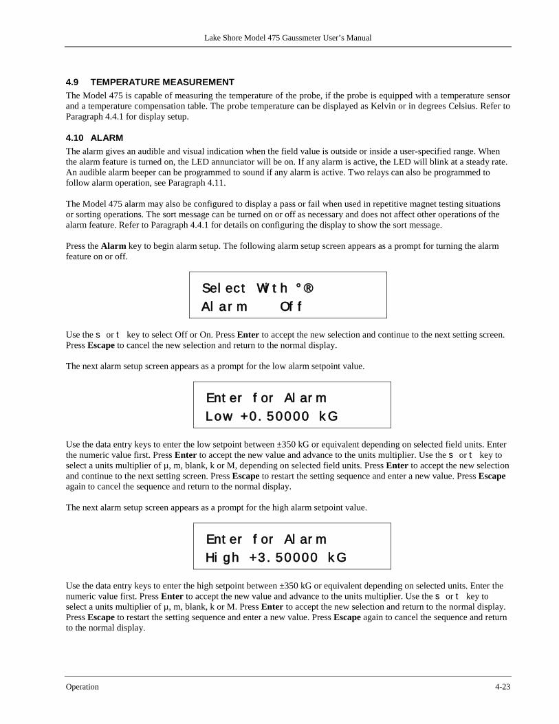
Lake Shore Model 475 Gaussmeter User’s Manual
Operation 4-23
4.9 TEMPERATURE MEASUREMENT The Model 475 is capable of measuring the temperature of the probe, if the probe is equipped with a temperature sensor and a temperature compensation table. The probe temperature can be displayed as Kelvin or in degrees Celsius. Refer to Paragraph 4.4.1 for display setup.
4.10 ALARM The alarm gives an audible and visual indication when the field value is outside or inside a user-specified range. When the alarm feature is turned on, the LED annunciator will be on. If any alarm is active, the LED will blink at a steady rate. An audible alarm beeper can be programmed to sound if any alarm is active. Two relays can also be programmed to follow alarm operation, see Paragraph 4.11. The Model 475 alarm may also be configured to display a pass or fail when used in repetitive magnet testing situations or sorting operations. The sort message can be turned on or off as necessary and does not affect other operations of the alarm feature. Refer to Paragraph 4.4.1 for details on configuring the display to show the sort message. Press the Alarm key to begin alarm setup. The following alarm setup screen appears as a prompt for turning the alarm feature on or off.
Sel ect Wi t h ° ® Al ar m Of f
Use the s or t key to select Off or On. Press Enter to accept the new selection and continue to the next setting screen. Press Escape to cancel the new selection and return to the normal display. The next alarm setup screen appears as a prompt for the low alarm setpoint value.
Ent er f or Al ar m Low +0. 50000 k G
Use the data entry keys to enter the low setpoint between ±350 kG or equivalent depending on selected field units. Enter the numeric value first. Press Enter to accept the new value and advance to the units multiplier. Use the s or t key to select a units multiplier of µ, m, blank, k or M, depending on selected field units. Press Enter to accept the new selection and continue to the next setting screen. Press Escape to restart the setting sequence and enter a new value. Press Escape again to cancel the sequence and return to the normal display. The next alarm setup screen appears as a prompt for the high alarm setpoint value.
Ent er f or Al ar m Hi gh +3 . 50000 k G
Use the data entry keys to enter the high setpoint between ±350 kG or equivalent depending on selected units. Enter the numeric value first. Press Enter to accept the new value and advance to the units multiplier. Use the s or t key to select a units multiplier of µ, m, blank, k or M. Press Enter to accept the new selection and return to the normal display. Press Escape to restart the setting sequence and enter a new value. Press Escape again to cancel the sequence and return to the normal display.

Lake Shore Model 475 Gaussmeter User’s Manual
4-24 Operation
The alarm may be configured to use the magnitude of the field reading only (ignoring the sign), or to include the sign and treat the readings algebraically. To configure the alarm for magnitude or algebraic mode, press and hold the Alarm key for approximately 4 seconds. The following alarm setup screen appears as a prompt for using the alarm in magnitude or algebraic mode.
Sel ect Wi t h ° ® Al ar m Magn i t ude
Use the s or t key to select from Magnitude or Algebraic. Press Enter to accept the new selection and continue to the next setting screen. Press Escape to cancel the new selection and return to the normal display. When the alarm feature is used to detect an error condition an active alarm state is expected when the field reading is higher than the high alarm setpoint or below the low alarm setpoint. This operation is achieved by setting the inside/outside parameter to outside. It is called outside because the alarm is active when the reading is outside the range of the two setpoints. During magnet testing or sorting it is often desirable to have the alarm active when the field reading is inside or between the two setpoints. This operation is achieved by setting the inside/outside parameter to inside. To configure the Alarm inside/outside setting, continue from the magnitude/algebraic mode screen or press and hold Alarm and then press Enter until the following screen appears as a prompt for selecting the inside/outside setting.
Sel ect Wi t h ° ® Al ar m I ns i de
Use the s or t key to select from Inside or Outside. Press Enter to accept the new selection and continue to the next setting screen. Press Escape to cancel the new selection and return to the normal display. The following images demonstrate different combinations of Inside/Outside with Magnitude or Algebraic measurements.
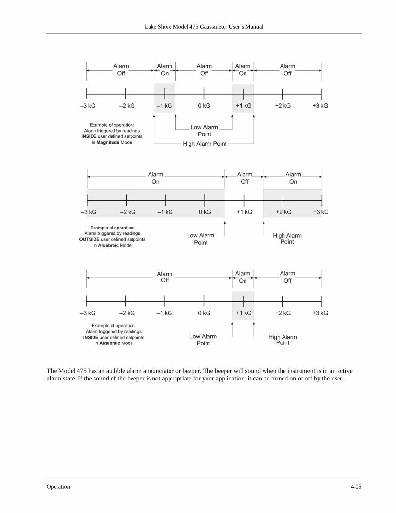
Lake Shore Model 475 Gaussmeter User’s Manual
Operation 4-25
The Model 475 has an audible alarm annunciator or beeper. The beeper will sound when the instrument is in an active alarm state. If the sound of the beeper is not appropriate for your application, it can be turned on or off by the user.
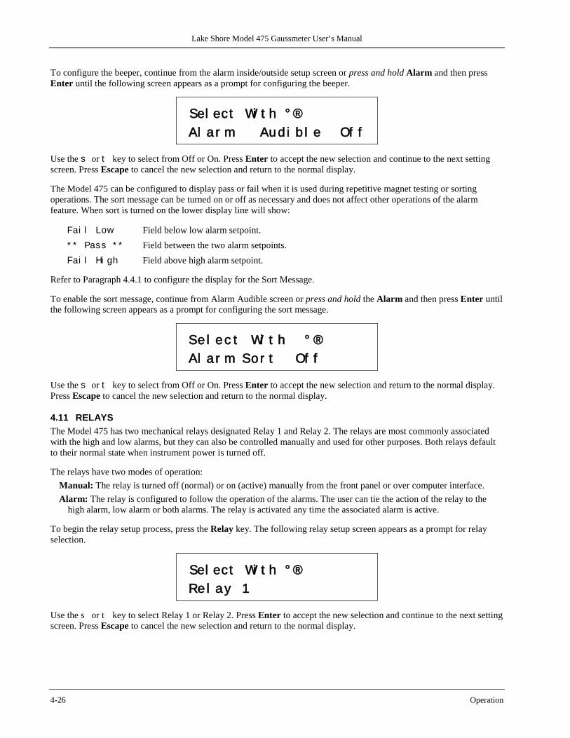
Lake Shore Model 475 Gaussmeter User’s Manual
4-26 Operation
To configure the beeper, continue from the alarm inside/outside setup screen or press and hold Alarm and then press Enter until the following screen appears as a prompt for configuring the beeper.
Sel ect Wi t h ° ® Al ar m Aud i b l e Of f
Use the s or t key to select from Off or On. Press Enter to accept the new selection and continue to the next setting screen. Press Escape to cancel the new selection and return to the normal display. The Model 475 can be configured to display pass or fail when it is used during repetitive magnet testing or sorting operations. The sort message can be turned on or off as necessary and does not affect other operations of the alarm feature. When sort is turned on the lower display line will show:
Fai l Low Field below low alarm setpoint. * * Pass * * Field between the two alarm setpoints. Fai l Hi gh Field above high alarm setpoint.
Refer to Paragraph 4.4.1 to configure the display for the Sort Message. To enable the sort message, continue from Alarm Audible screen or press and hold the Alarm and then press Enter until the following screen appears as a prompt for configuring the sort message.
Se l ec t Wi t h ° ® Al ar m Sor t Of f
Use the s or t key to select from Off or On. Press Enter to accept the new selection and return to the normal display. Press Escape to cancel the new selection and return to the normal display.
4.11 RELAYS The Model 475 has two mechanical relays designated Relay 1 and Relay 2. The relays are most commonly associated with the high and low alarms, but they can also be controlled manually and used for other purposes. Both relays default to their normal state when instrument power is turned off. The relays have two modes of operation:
Manual: The relay is turned off (normal) or on (active) manually from the front panel or over computer interface. Alarm: The relay is configured to follow the operation of the alarms. The user can tie the action of the relay to the
high alarm, low alarm or both alarms. The relay is activated any time the associated alarm is active. To begin the relay setup process, press the Relay key. The following relay setup screen appears as a prompt for relay selection.
Sel ect Wi t h ° ® Re l ay 1
Use the s or t key to select Relay 1 or Relay 2. Press Enter to accept the new selection and continue to the next setting screen. Press Escape to cancel the new selection and return to the normal display.
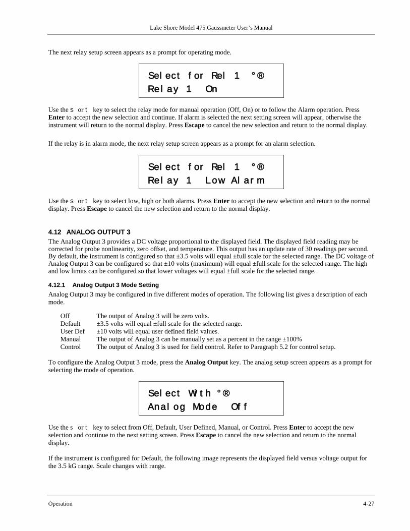
Lake Shore Model 475 Gaussmeter User’s Manual
Operation 4-27
The next relay setup screen appears as a prompt for operating mode.
Sel ect f or Rel 1 ° ® Re l ay 1 On
Use the s or t key to select the relay mode for manual operation (Off, On) or to follow the Alarm operation. Press Enter to accept the new selection and continue. If alarm is selected the next setting screen will appear, otherwise the instrument will return to the normal display. Press Escape to cancel the new selection and return to the normal display.
If the relay is in alarm mode, the next relay setup screen appears as a prompt for an alarm selection.
Sel ect f or Rel 1 ° ® Re l ay 1 Low Al a r m
Use the s or t key to select low, high or both alarms. Press Enter to accept the new selection and return to the normal display. Press Escape to cancel the new selection and return to the normal display.
4.12 ANALOG OUTPUT 3 The Analog Output 3 provides a DC voltage proportional to the displayed field. The displayed field reading may be corrected for probe nonlinearity, zero offset, and temperature. This output has an update rate of 30 readings per second. By default, the instrument is configured so that ±3.5 volts will equal ±full scale for the selected range. The DC voltage of Analog Output 3 can be configured so that ±10 volts (maximum) will equal ±full scale for the selected range. The high and low limits can be configured so that lower voltages will equal ±full scale for the selected range.
4.12.1 Analog Output 3 Mode Setting Analog Output 3 may be configured in five different modes of operation. The following list gives a description of each mode.
Off The output of Analog 3 will be zero volts. Default ±3.5 volts will equal ±full scale for the selected range. User Def ±10 volts will equal user defined field values. Manual The output of Analog 3 can be manually set as a percent in the range ±100% Control The output of Analog 3 is used for field control. Refer to Paragraph 5.2 for control setup.
To configure the Analog Output 3 mode, press the Analog Output key. The analog setup screen appears as a prompt for selecting the mode of operation.
Sel ect Wi t h ° ® Ana l og Mode Of f
Use the s or t key to select from Off, Default, User Defined, Manual, or Control. Press Enter to accept the new selection and continue to the next setting screen. Press Escape to cancel the new selection and return to the normal display. If the instrument is configured for Default, the following image represents the displayed field versus voltage output for the 3.5 kG range. Scale changes with range.
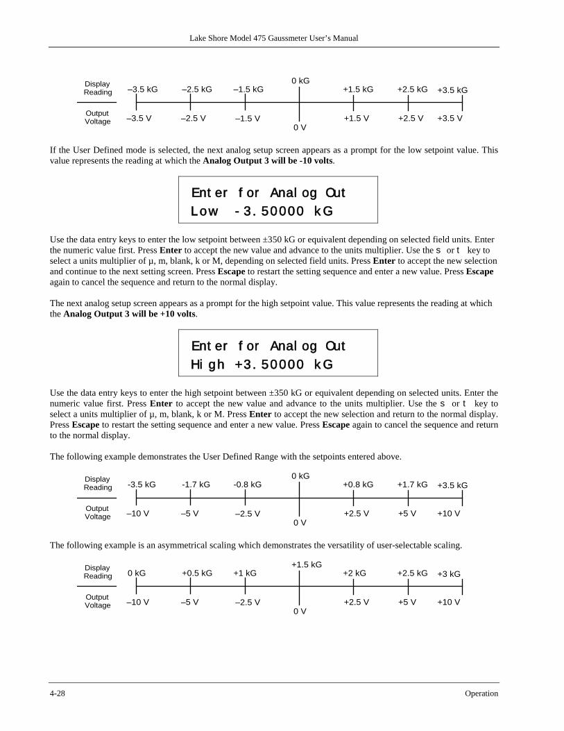
Lake Shore Model 475 Gaussmeter User’s Manual
4-28 Operation
0 V +1.5 V +2.5 V +3.5 V –3.5 V –2.5 V –1.5 V
0 kG +1.5 kG +2.5 kG +3.5 kG –3.5 kG –2.5 kG –1.5 kG Display
Reading
Output Voltage
If the User Defined mode is selected, the next analog setup screen appears as a prompt for the low setpoint value. This value represents the reading at which the Analog Output 3 will be -10 volts.
Ent er f or Anal og Out Low - 3 . 50000 k G
Use the data entry keys to enter the low setpoint between ±350 kG or equivalent depending on selected field units. Enter the numeric value first. Press Enter to accept the new value and advance to the units multiplier. Use the s or t key to select a units multiplier of µ, m, blank, k or M, depending on selected field units. Press Enter to accept the new selection and continue to the next setting screen. Press Escape to restart the setting sequence and enter a new value. Press Escape again to cancel the sequence and return to the normal display. The next analog setup screen appears as a prompt for the high setpoint value. This value represents the reading at which the Analog Output 3 will be +10 volts.
Ent er f or Anal og Out Hi gh +3 . 50000 k G
Use the data entry keys to enter the high setpoint between ±350 kG or equivalent depending on selected units. Enter the numeric value first. Press Enter to accept the new value and advance to the units multiplier. Use the s or t key to select a units multiplier of µ, m, blank, k or M. Press Enter to accept the new selection and return to the normal display. Press Escape to restart the setting sequence and enter a new value. Press Escape again to cancel the sequence and return to the normal display. The following example demonstrates the User Defined Range with the setpoints entered above.
0 V +2.5 V +5 V +10 V –10 V –5 V –2.5 V
0 kG +0.8 kG +1.7 kG +3.5 kG -3.5 kG -1.7 kG -0.8 kG Display
Reading
Output Voltage
The following example is an asymmetrical scaling which demonstrates the versatility of user-selectable scaling.
0 V +2.5 V +5 V +10 V –10 V –5 V –2.5 V
+1.5 kG +2 kG +2.5 kG +3 kG 0 kG +0.5 kG +1 kG Display
Reading
Output Voltage
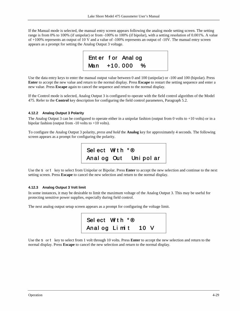
Lake Shore Model 475 Gaussmeter User’s Manual
Operation 4-29
If the Manual mode is selected, the manual entry screen appears following the analog mode setting screen. The setting range is from 0% to 100% (if unipolar) or from -100% to 100% (if bipolar), with a setting resolution of 0.001%. A value of +100% represents an output of 10 V and a value of -100% represents an output of -10V. The manual entry screen appears as a prompt for setting the Analog Output 3 voltage.
Ent er f or Anal og Man +10 . 000 %
Use the data entry keys to enter the manual output value between 0 and 100 (unipolar) or -100 and 100 (bipolar). Press Enter to accept the new value and return to the normal display. Press Escape to restart the setting sequence and enter a new value. Press Escape again to cancel the sequence and return to the normal display. If the Control mode is selected, Analog Output 3 is configured to operate with the field control algorithm of the Model 475. Refer to the Control key description for configuring the field control parameters, Paragraph 5.2.
4.12.2 Analog Output 3 Polarity The Analog Output 3 can be configured to operate either in a unipolar fashion (output from 0 volts to +10 volts) or in a bipolar fashion (output from -10 volts to +10 volts). To configure the Analog Output 3 polarity, press and hold the Analog key for approximately 4 seconds. The following screen appears as a prompt for configuring the polarity.
Sel ect Wi t h ° ® Ana l og Out Un i po l a r
Use the s or t key to select from Unipolar or Bipolar. Press Enter to accept the new selection and continue to the next setting screen. Press Escape to cancel the new selection and return to the normal display.
4.12.3 Analog Output 3 Volt limit In some instances, it may be desirable to limit the maximum voltage of the Analog Output 3. This may be useful for protecting sensitive power supplies, especially during field control. The next analog output setup screen appears as a prompt for configuring the voltage limit.
Sel ect Wi t h ° ® Ana l og L i mi t 10 V
Use the s or t key to select from 1 volt through 10 volts. Press Enter to accept the new selection and return to the normal display. Press Escape to cancel the new selection and return to the normal display.
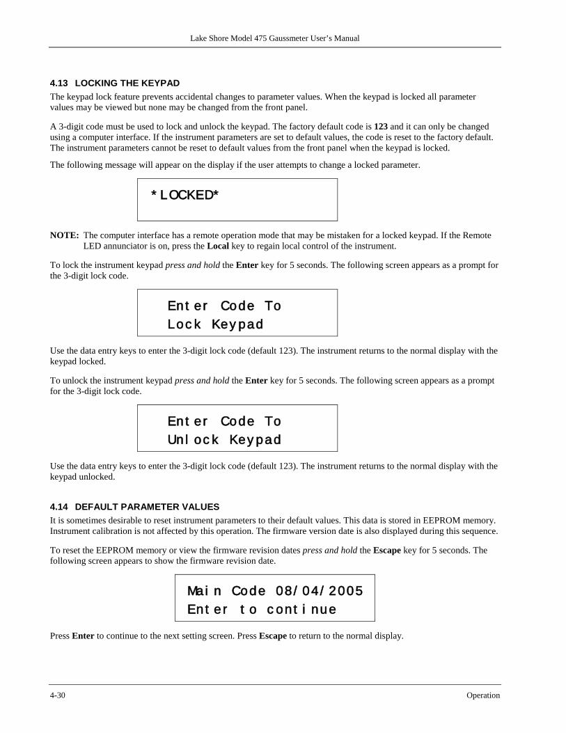
Lake Shore Model 475 Gaussmeter User’s Manual
4-30 Operation
4.13 LOCKING THE KEYPAD The keypad lock feature prevents accidental changes to parameter values. When the keypad is locked all parameter values may be viewed but none may be changed from the front panel. A 3-digit code must be used to lock and unlock the keypad. The factory default code is 123 and it can only be changed using a computer interface. If the instrument parameters are set to default values, the code is reset to the factory default. The instrument parameters cannot be reset to default values from the front panel when the keypad is locked.
The following message will appear on the display if the user attempts to change a locked parameter.
* LOCKED*
NOTE: The computer interface has a remote operation mode that may be mistaken for a locked keypad. If the Remote
LED annunciator is on, press the Local key to regain local control of the instrument. To lock the instrument keypad press and hold the Enter key for 5 seconds. The following screen appears as a prompt for the 3-digit lock code.
En t er Code To Loc k Key pad
Use the data entry keys to enter the 3-digit lock code (default 123). The instrument returns to the normal display with the keypad locked. To unlock the instrument keypad press and hold the Enter key for 5 seconds. The following screen appears as a prompt for the 3-digit lock code.
En t er Code To Un l oc k Key pad
Use the data entry keys to enter the 3-digit lock code (default 123). The instrument returns to the normal display with the keypad unlocked.
4.14 DEFAULT PARAMETER VALUES It is sometimes desirable to reset instrument parameters to their default values. This data is stored in EEPROM memory. Instrument calibration is not affected by this operation. The firmware version date is also displayed during this sequence. To reset the EEPROM memory or view the firmware revision dates press and hold the Escape key for 5 seconds. The following screen appears to show the firmware revision date.
Mai n Code 08/ 04/ 2005 En t e r t o c ont i nue
Press Enter to continue to the next setting screen. Press Escape to return to the normal display.
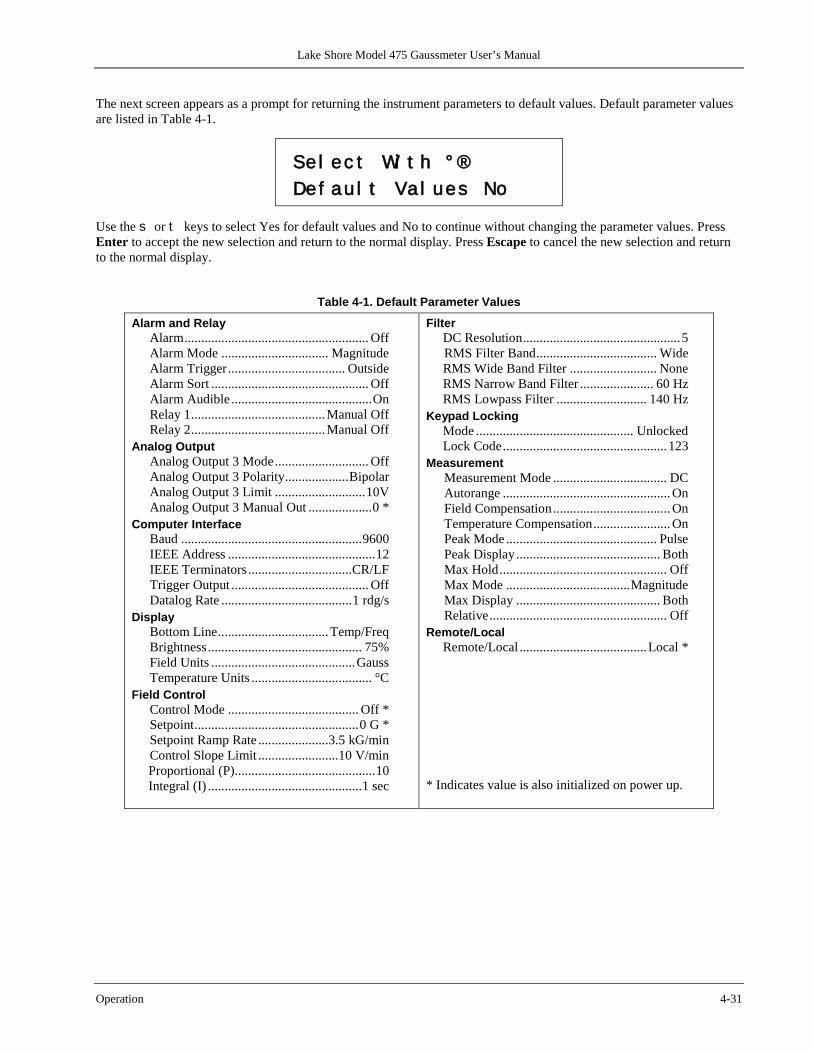
Lake Shore Model 475 Gaussmeter User’s Manual
Operation 4-31
The next screen appears as a prompt for returning the instrument parameters to default values. Default parameter values are listed in Table 4-1.
Se l ec t Wi t h ° ® De f au l t Va l ues No
Use the s or t keys to select Yes for default values and No to continue without changing the parameter values. Press Enter to accept the new selection and return to the normal display. Press Escape to cancel the new selection and return to the normal display.
Table 4-1. Default Parameter Values Alarm and Relay
Alarm ....................................................... Off Alarm Mode ................................ Magnitude Alarm Trigger ................................... Outside Alarm Sort ............................................... Off Alarm Audible .......................................... On Relay 1 ........................................ Manual Off Relay 2 ........................................ Manual Off
Analog Output Analog Output 3 Mode ............................ Off Analog Output 3 Polarity ................... Bipolar Analog Output 3 Limit ........................... 10V Analog Output 3 Manual Out ................... 0 *
Computer Interface Baud ...................................................... 9600 IEEE Address ............................................ 12 IEEE Terminators ............................... CR/LF Trigger Output ......................................... Off Datalog Rate ....................................... 1 rdg/s
Display Bottom Line ................................. Temp/Freq Brightness .............................................. 75% Field Units ........................................... Gauss Temperature Units .................................... °C
Field Control Control Mode ....................................... Off * Setpoint ................................................. 0 G * Setpoint Ramp Rate .....................3.5 kG/min Control Slope Limit ........................10 V/min Proportional (P) .......................................... 10 Integral (I) .............................................. 1 sec
Filter DC Resolution ............................................... 5 RMS Filter Band .................................... Wide RMS Wide Band Filter .......................... None RMS Narrow Band Filter ...................... 60 Hz RMS Lowpass Filter ........................... 140 Hz
Keypad Locking Mode ............................................... Unlocked Lock Code ................................................. 123
Measurement Measurement Mode .................................. DC Autorange .................................................. On Field Compensation ................................... On Temperature Compensation ....................... On Peak Mode ............................................. Pulse Peak Display ........................................... Both Max Hold .................................................. Off Max Mode ..................................... Magnitude Max Display ........................................... Both Relative ..................................................... Off
Remote/Local Remote/Local ...................................... Local *
* Indicates value is also initialized on power up.

Lake Shore Model 475 Gaussmeter User’s Manual
4-32 Operation
This Page Intentionally Left Blank
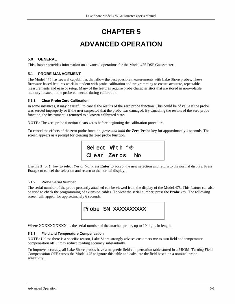
Lake Shore Model 475 Gaussmeter User’s Manual
Advanced Operation 5-1
CHAPTER 5
ADVANCED OPERATION
5.0 GENERAL This chapter provides information on advanced operations for the Model 475 DSP Gaussmeter.
5.1 PROBE MANAGEMENT The Model 475 has several capabilities that allow the best possible measurements with Lake Shore probes. These firmware-based features work in tandem with probe calibration and programming to ensure accurate, repeatable measurements and ease of setup. Many of the features require probe characteristics that are stored in non-volatile memory located in the probe connector during calibration.
5.1.1 Clear Probe Zero Calibration In some instances, it may be useful to cancel the results of the zero probe function. This could be of value if the probe was zeroed improperly or if the user suspected that the probe was damaged. By canceling the results of the zero probe function, the instrument is returned to a known calibrated state. NOTE: The zero probe function clears zeros before beginning the calibration procedure. To cancel the effects of the zero probe function, press and hold the Zero Probe key for approximately 4 seconds. The screen appears as a prompt for clearing the zero probe function.
Sel ect Wi t h ° ® Cl ea r Ze r os No
Use the s or t key to select Yes or No. Press Enter to accept the new selection and return to the normal display. Press Escape to cancel the selection and return to the normal display.
5.1.2 Probe Serial Number The serial number of the probe presently attached can be viewed from the display of the Model 475. This feature can also be used to check the programming of extension cables. To view the serial number, press the Probe key. The following screen will appear for approximately 6 seconds.
Pr obe SN XXXXXXXXXX
Where XXXXXXXXXX, is the serial number of the attached probe, up to 10 digits in length.
5.1.3 Field and Temperature Compensation NOTE: Unless there is a specific reason, Lake Shore strongly advises customers not to turn field and temperature compensation off; it may reduce reading accuracy substantially.
To improve accuracy, all Lake Shore probes have a magnetic field compensation table stored in a PROM. Turning Field Compensation OFF causes the Model 475 to ignore this table and calculate the field based on a nominal probe sensitivity.

Lake Shore Model 475 Gaussmeter User’s Manual
5-2 Advanced Operation
Some probes also feature temperature compensation. Turning Temperature Compensation OFF causes the Model 475 to ignore this data. To configure the Field Compensation setting, press the Probe key and wait until the Probe Serial number display disappears and the following screen appears as a prompt for field compensation.
Sel ect Wi t h ° ® Fi e l d Comp Of f
Use the s or t key to select Off or On. Press Enter to accept the new selection and continue to the next setting screen. Press Escape to cancel the selection and return to the normal display. The next probe setting screen appears as a prompt for changing the temperature compensation setting.
Sel ect Wi t h ° ® Temp Comp Of f
Use the s or t key to select Off or On. Press Enter to accept the new selection and return to the normal display. Press Escape to cancel the selection and return to the normal display. If the probe does not include temperature compensation, this setting is ignored.
5.1.4 Extension Cable The complex nature of Hall-effect measurements makes it necessary to match extension cables to the probe when longer cables are needed. Keeping probes and their extensions from getting mixed up can become a problem when more than one probe is in use. The Model 475 alleviates some of the difficulty by allowing users to match probes to extensions in the field. Stored information can be viewed on the front panel and read over computer interface to ensure proper mating. NOTE: Calibrated probe and extension cable pairs may be purchased from Lake Shore and are recommended for the best accuracy. Extension cables with no calibration may also be used. The Model 475 can then be used to match a probe to the un-calibrated extension cable. To match a probe with an extension cable, verify that the probe is connected to the instrument. To begin the matching process, press and hold the Probe key for approximately 4 seconds. The following screen appears as a prompt for selecting the programming method.
Sel ect Wi t h ° ® MPEC Pr ogr am
Use the s or t key to select from MPEC program (extension cables) or MCBL Program (User programmable cables, refer to Paragraph 5.2.1). Press Enter to accept the new selection and continue the matching process. Press Escape to cancel the selection and return to the normal display. The next probe matching screen appears as a prompt to begin the copying process.
At t ach MPEC cabl e En t e r t o Cont i nue
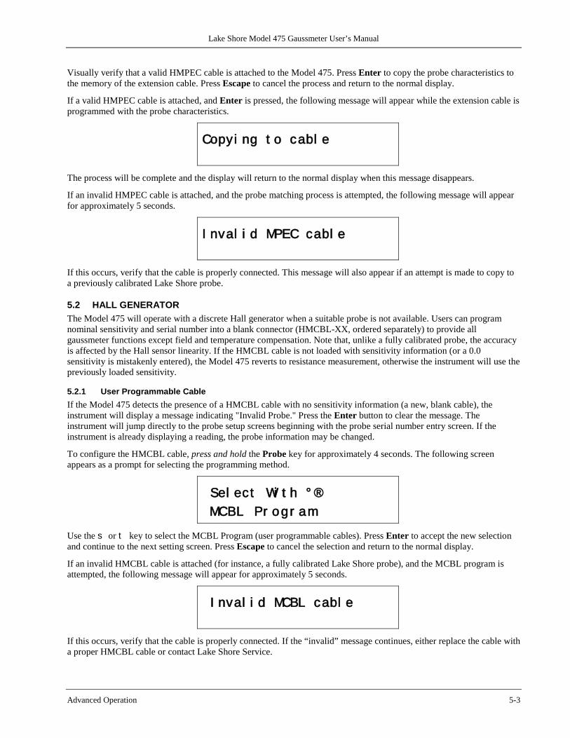
Lake Shore Model 475 Gaussmeter User’s Manual
Advanced Operation 5-3
Visually verify that a valid HMPEC cable is attached to the Model 475. Press Enter to copy the probe characteristics to the memory of the extension cable. Press Escape to cancel the process and return to the normal display.
If a valid HMPEC cable is attached, and Enter is pressed, the following message will appear while the extension cable is programmed with the probe characteristics.
Copyi ng t o cabl e
The process will be complete and the display will return to the normal display when this message disappears.
If an invalid HMPEC cable is attached, and the probe matching process is attempted, the following message will appear for approximately 5 seconds.
I nval i d MPEC cabl e
If this occurs, verify that the cable is properly connected. This message will also appear if an attempt is made to copy to a previously calibrated Lake Shore probe.
5.2 HALL GENERATOR The Model 475 will operate with a discrete Hall generator when a suitable probe is not available. Users can program nominal sensitivity and serial number into a blank connector (HMCBL-XX, ordered separately) to provide all gaussmeter functions except field and temperature compensation. Note that, unlike a fully calibrated probe, the accuracy is affected by the Hall sensor linearity. If the HMCBL cable is not loaded with sensitivity information (or a 0.0 sensitivity is mistakenly entered), the Model 475 reverts to resistance measurement, otherwise the instrument will use the previously loaded sensitivity.
5.2.1 User Programmable Cable If the Model 475 detects the presence of a HMCBL cable with no sensitivity information (a new, blank cable), the instrument will display a message indicating "Invalid Probe." Press the Enter button to clear the message. The instrument will jump directly to the probe setup screens beginning with the probe serial number entry screen. If the instrument is already displaying a reading, the probe information may be changed.
To configure the HMCBL cable, press and hold the Probe key for approximately 4 seconds. The following screen appears as a prompt for selecting the programming method.
Sel ect Wi t h ° ® MCBL Pr ogr am
Use the s or t key to select the MCBL Program (user programmable cables). Press Enter to accept the new selection and continue to the next setting screen. Press Escape to cancel the selection and return to the normal display.
If an invalid HMCBL cable is attached (for instance, a fully calibrated Lake Shore probe), and the MCBL program is attempted, the following message will appear for approximately 5 seconds.
I nval i d MCBL cabl e
If this occurs, verify that the cable is properly connected. If the “invalid” message continues, either replace the cable with a proper HMCBL cable or contact Lake Shore Service.
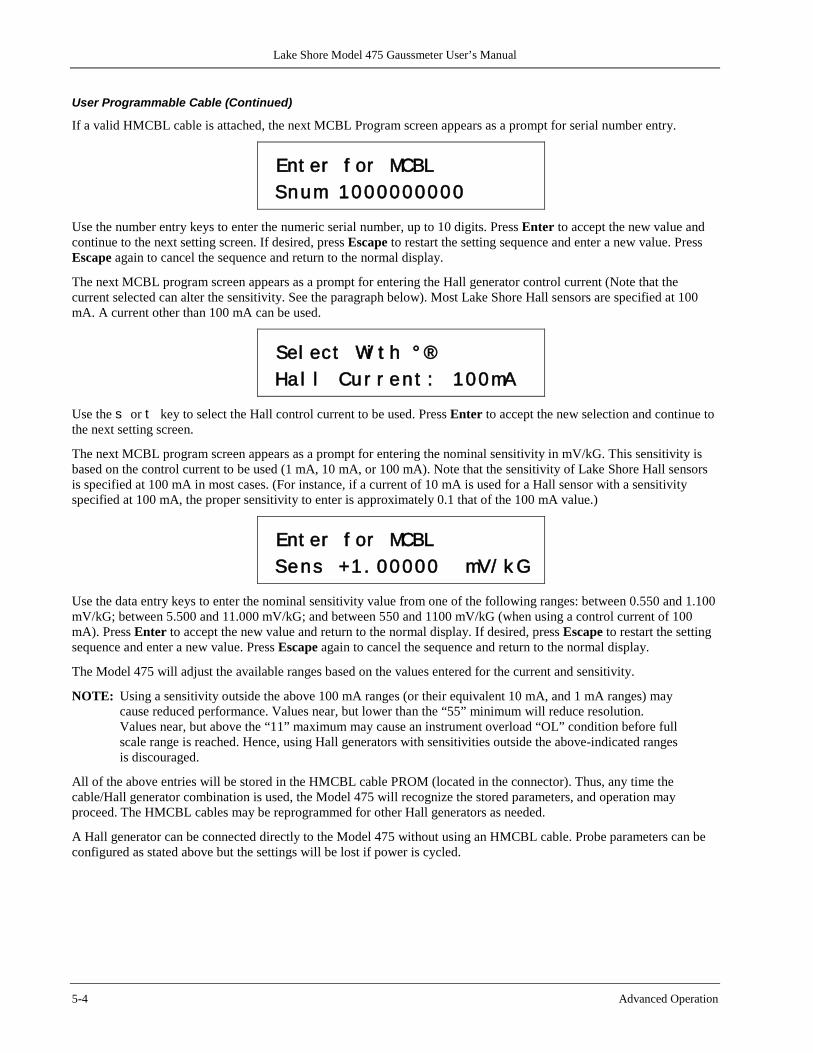
Lake Shore Model 475 Gaussmeter User’s Manual
5-4 Advanced Operation
User Programmable Cable (Continued)
If a valid HMCBL cable is attached, the next MCBL Program screen appears as a prompt for serial number entry.
Ent er f or MCBL Snum 1000000000
Use the number entry keys to enter the numeric serial number, up to 10 digits. Press Enter to accept the new value and continue to the next setting screen. If desired, press Escape to restart the setting sequence and enter a new value. Press Escape again to cancel the sequence and return to the normal display.
The next MCBL program screen appears as a prompt for entering the Hall generator control current (Note that the current selected can alter the sensitivity. See the paragraph below). Most Lake Shore Hall sensors are specified at 100 mA. A current other than 100 mA can be used.
Sel ect Wi t h ° ® Ha l l Cur r en t : 100mA
Use the s or t key to select the Hall control current to be used. Press Enter to accept the new selection and continue to the next setting screen.
The next MCBL program screen appears as a prompt for entering the nominal sensitivity in mV/kG. This sensitivity is based on the control current to be used (1 mA, 10 mA, or 100 mA). Note that the sensitivity of Lake Shore Hall sensors is specified at 100 mA in most cases. (For instance, if a current of 10 mA is used for a Hall sensor with a sensitivity specified at 100 mA, the proper sensitivity to enter is approximately 0.1 that of the 100 mA value.)
Ent er f or MCBL Sens +1 . 00000 mV/ k G
Use the data entry keys to enter the nominal sensitivity value from one of the following ranges: between 0.550 and 1.100 mV/kG; between 5.500 and 11.000 mV/kG; and between 550 and 1100 mV/kG (when using a control current of 100 mA). Press Enter to accept the new value and return to the normal display. If desired, press Escape to restart the setting sequence and enter a new value. Press Escape again to cancel the sequence and return to the normal display.
The Model 475 will adjust the available ranges based on the values entered for the current and sensitivity.
NOTE: Using a sensitivity outside the above 100 mA ranges (or their equivalent 10 mA, and 1 mA ranges) may cause reduced performance. Values near, but lower than the “55” minimum will reduce resolution. Values near, but above the “11” maximum may cause an instrument overload “OL” condition before full scale range is reached. Hence, using Hall generators with sensitivities outside the above-indicated ranges is discouraged.
All of the above entries will be stored in the HMCBL cable PROM (located in the connector). Thus, any time the cable/Hall generator combination is used, the Model 475 will recognize the stored parameters, and operation may proceed. The HMCBL cables may be reprogrammed for other Hall generators as needed.
A Hall generator can be connected directly to the Model 475 without using an HMCBL cable. Probe parameters can be configured as stated above but the settings will be lost if power is cycled.
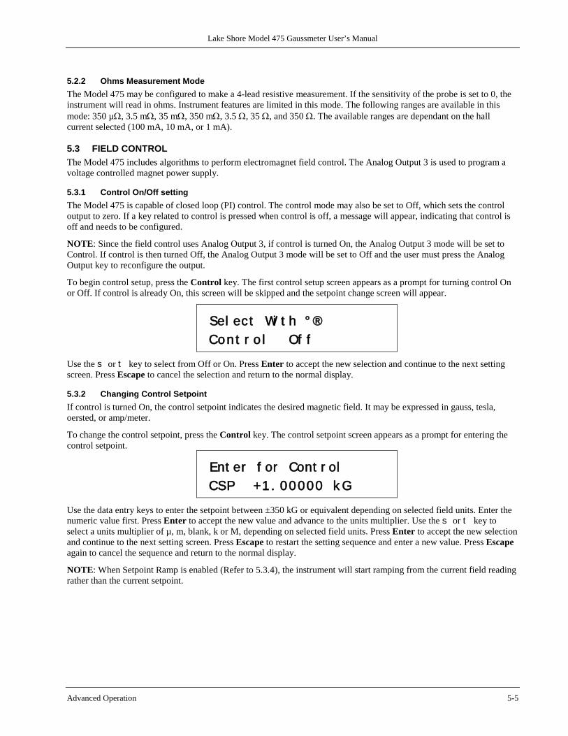
Lake Shore Model 475 Gaussmeter User’s Manual
Advanced Operation 5-5
5.2.2 Ohms Measurement Mode The Model 475 may be configured to make a 4-lead resistive measurement. If the sensitivity of the probe is set to 0, the instrument will read in ohms. Instrument features are limited in this mode. The following ranges are available in this mode: 350 µΩ, 3.5 mΩ, 35 mΩ, 350 mΩ, 3.5 Ω, 35 Ω, and 350 Ω. The available ranges are dependant on the hall current selected (100 mA, 10 mA, or 1 mA).
5.3 FIELD CONTROL The Model 475 includes algorithms to perform electromagnet field control. The Analog Output 3 is used to program a voltage controlled magnet power supply.
5.3.1 Control On/Off setting The Model 475 is capable of closed loop (PI) control. The control mode may also be set to Off, which sets the control output to zero. If a key related to control is pressed when control is off, a message will appear, indicating that control is off and needs to be configured.
NOTE: Since the field control uses Analog Output 3, if control is turned On, the Analog Output 3 mode will be set to Control. If control is then turned Off, the Analog Output 3 mode will be set to Off and the user must press the Analog Output key to reconfigure the output.
To begin control setup, press the Control key. The first control setup screen appears as a prompt for turning control On or Off. If control is already On, this screen will be skipped and the setpoint change screen will appear.
Sel ect Wi t h ° ® Cont r o l Of f
Use the s or t key to select from Off or On. Press Enter to accept the new selection and continue to the next setting screen. Press Escape to cancel the selection and return to the normal display.
5.3.2 Changing Control Setpoint If control is turned On, the control setpoint indicates the desired magnetic field. It may be expressed in gauss, tesla, oersted, or amp/meter.
To change the control setpoint, press the Control key. The control setpoint screen appears as a prompt for entering the control setpoint.
Ent er f or Cont r ol CSP +1 . 00000 k G
Use the data entry keys to enter the setpoint between ±350 kG or equivalent depending on selected field units. Enter the numeric value first. Press Enter to accept the new value and advance to the units multiplier. Use the s or t key to select a units multiplier of µ, m, blank, k or M, depending on selected field units. Press Enter to accept the new selection and continue to the next setting screen. Press Escape to restart the setting sequence and enter a new value. Press Escape again to cancel the sequence and return to the normal display.
NOTE: When Setpoint Ramp is enabled (Refer to 5.3.4), the instrument will start ramping from the current field reading rather than the current setpoint.
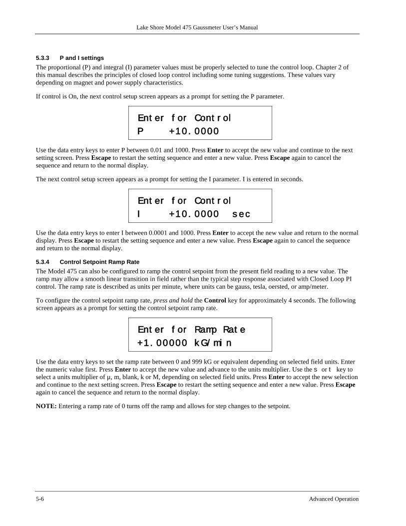
Lake Shore Model 475 Gaussmeter User’s Manual
5-6 Advanced Operation
5.3.3 P and I settings The proportional (P) and integral (I) parameter values must be properly selected to tune the control loop. Chapter 2 of this manual describes the principles of closed loop control including some tuning suggestions. These values vary depending on magnet and power supply characteristics. If control is On, the next control setup screen appears as a prompt for setting the P parameter.
Ent er f or Cont r ol P +10 . 0000
Use the data entry keys to enter P between 0.01 and 1000. Press Enter to accept the new value and continue to the next setting screen. Press Escape to restart the setting sequence and enter a new value. Press Escape again to cancel the sequence and return to the normal display. The next control setup screen appears as a prompt for setting the I parameter. I is entered in seconds.
Ent er f or Cont r ol I +10 . 0000 s ec
Use the data entry keys to enter I between 0.0001 and 1000. Press Enter to accept the new value and return to the normal display. Press Escape to restart the setting sequence and enter a new value. Press Escape again to cancel the sequence and return to the normal display.
5.3.4 Control Setpoint Ramp Rate The Model 475 can also be configured to ramp the control setpoint from the present field reading to a new value. The ramp may allow a smooth linear transition in field rather than the typical step response associated with Closed Loop PI control. The ramp rate is described as units per minute, where units can be gauss, tesla, oersted, or amp/meter. To configure the control setpoint ramp rate, press and hold the Control key for approximately 4 seconds. The following screen appears as a prompt for setting the control setpoint ramp rate.
Ent er f or Ramp Rat e +1 . 00000 k G/ mi n
Use the data entry keys to set the ramp rate between 0 and 999 kG or equivalent depending on selected field units. Enter the numeric value first. Press Enter to accept the new value and advance to the units multiplier. Use the s or t key to select a units multiplier of µ, m, blank, k or M, depending on selected field units. Press Enter to accept the new selection and continue to the next setting screen. Press Escape to restart the setting sequence and enter a new value. Press Escape again to cancel the sequence and return to the normal display. NOTE: Entering a ramp rate of 0 turns off the ramp and allows for step changes to the setpoint.
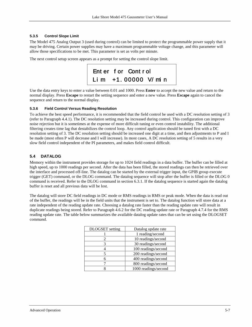
Lake Shore Model 475 Gaussmeter User’s Manual
Advanced Operation 5-7
5.3.5 Control Slope Limit The Model 475 Analog Output 3 (used during control) can be limited to protect the programmable power supply that it may be driving. Certain power supplies may have a maximum programmable voltage change, and this parameter will allow those specifications to be met. This parameter is set as volts per minute.
The next control setup screen appears as a prompt for setting the control slope limit.
Ent er f or Cont r ol L i m +1 . 00000 V/ mi n
Use the data entry keys to enter a value between 0.01 and 1000. Press Enter to accept the new value and return to the normal display. Press Escape to restart the setting sequence and enter a new value. Press Escape again to cancel the sequence and return to the normal display.
5.3.6 Field Control Versus Reading Resolution To achieve the best speed performance, it is recommended that the field control be used with a DC resolution setting of 3 (refer to Paragraph 4.4.1). The DC resolution setting may be increased during control. This configuration can improve noise rejection but it is sometimes at the expense of more difficult tuning or even control instability. The additional filtering creates time lag that destabilizes the control loop. Any control application should be tuned first with a DC resolution setting of 3. The DC resolution setting should be increased one digit at a time, and then adjustments to P and I be made (most often P will decrease and I will increase). In most cases, A DC resolution setting of 5 results in a very slow field control independent of the PI parameters, and makes field control difficult.
5.4 DATALOG Memory within the instrument provides storage for up to 1024 field readings in a data buffer. The buffer can be filled at high speed, up to 1000 readings per second. After the data has been filled, the stored readings can then be retrieved over the interface and processed off-line. The datalog can be started by the external trigger input, the GPIB group execute trigger (GET) command, or the DLOG command. The datalog sequence will stop after the buffer is filled or the DLOG 0 command is received. Refer to the DLOG command in section 6.3.1. If the datalog sequence is started again the datalog buffer is reset and all previous data will be lost. The datalog will store DC field readings in DC mode or RMS readings in RMS or peak mode. When the data is read out of the buffer, the readings will be in the field units that the instrument is set to. The datalog function will store data at a rate independent of the reading update rate. Choosing a datalog rate faster than the reading update rate will result in duplicate readings being stored. Refer to Paragraph 4.6.2 for the DC reading update rate or Paragraph 4.7.4 for the RMS reading update rate. The table below summarizes the available datalog update rates that can be set using the DLOGSET command.
DLOGSET setting Datalog update rate 1 1 reading/second 2 10 readings/second 3 30 readings/second 4 100 readings/second 5 200 readings/second 6 400 readings/second 7 800 readings/second 8 1000 readings/second

Lake Shore Model 475 Gaussmeter User’s Manual
5-8 Advanced Operation
5.5 TRIGGERING A hardware, TTL level, trigger into the instrument can be used to initiate the data log sequence. A hardware, TTL level trigger out of the instrument indicates when the instrument completes a reading and can be used to synchronize other instruments in a system. A software, IEEE-488 based trigger can be used similar to the hardware trigger in. The hardware trigger signals are located in the Auxiliary I/O connector, which is described in Paragraph 3.6. The timing of the hardware trigger input and output are described in Figures 5-1 and 5-2. The hardware trigger input is an edge sensitive, active low signal. To ensure that the trigger is detected by the Model 475, it is recommended that the signal be held high for a minimum of 25 microseconds, and then held low for another 25 microseconds before going high again. The hardware trigger output is a 2 millisecond, active low, pulse. This signal is not available during the high speed binary operation of the instrument (refer to Chapter 6 for high speed binary description).
Figure 5-1. Trigger Input Timing Diagram
Figure 5-2. Trigger Output Timing Diagram
Lake Shore Model 475 Gaussmeter User’s Manual
Remote Operation 6-1
CHAPTER 6
COMPUTER INTERFACE OPERATION
6.0 GENERAL This chapter provides operational instructions for the computer interface for the Lake Shore Model 475 Gaussmeter. Either of the two computer interfaces provided with the Model 475 permit remote operation. The first is the IEEE-488 Interface described in Paragraph 6.1. The second is the Serial Interface described in Paragraph 6.2. The two interfaces share a common set of commands detailed in Paragraph 6.3. Only one of the interfaces can be used at a time.
6.1 IEEE-488 INTERFACE The IEEE-488 Interface is an instrumentation bus with hardware and programming standards that simplify instrument interfacing. The Model 475 IEEE-488 Interface complies with the IEEE-488.2-1987 standard and incorporates its functional, electrical, and mechanical specifications unless otherwise specified in this manual. All instruments on the interface bus perform one or more of the interface functions of TALKER, LISTENER, or BUS CONTROLLER. A TALKER transmits data onto the bus to other devices. A LISTENER receives data from other devices through the bus. The BUS CONTROLLER designates to the devices on the bus which function to perform. The Model 475 performs the functions of TALKER and LISTENER but cannot be a BUS CONTROLLER. The BUS CONTROLLER is the digital computer which tells the Model 475 which functions to perform. Below are Model 475 IEEE-488 interface capabilities:
• SH1: Source handshake capability. • RL1: Complete remote/local capability. • DC1: Full device clear capability. • DT1: Complete device trigger capability. • C0: No system controller capability. • T5: Basic TALKER, serial poll capability, talk only, unaddressed to talk if addressed to listen. • L4: Basic LISTENER, unaddressed to listen if addressed to talk. • SR1: Service request capability. • AH1: Acceptor handshake capability. • PP0: No parallel poll capability. • E1: Open collector electronics.
NOTE: The Model 475 IEEE-488 Interface requires that repeat addressing be enabled on the bus controller. Instruments are connected to the IEEE-488 bus by a 24-conductor connector cable as specified by the standard. Refer to Paragraph 8.11.2. Cables can be purchased from Lake Shore or other electronic suppliers. A connector extender (Model 4005) is required to use the IEEE-488 Interface and the Auxiliary connector at the same time. Cable lengths are limited to 2 meters for each device and 20 meters for the entire bus. The Model 475 can drive a bus with up to 10 loads. If more instruments or cable length is required, a bus expander must be used.
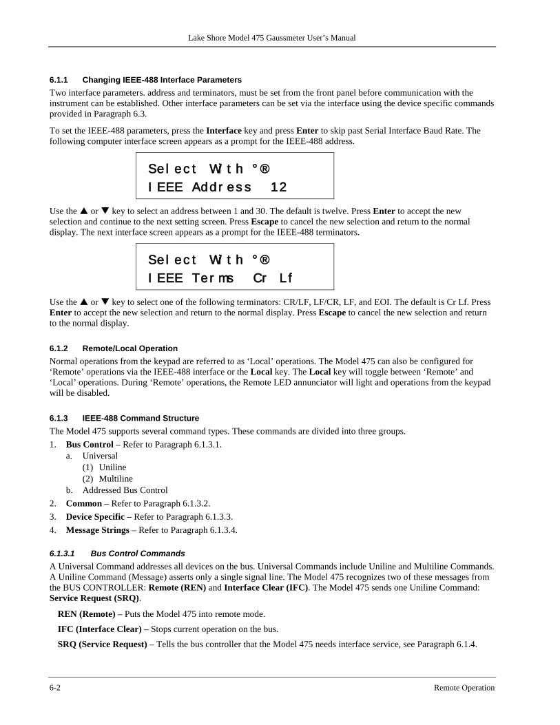
Lake Shore Model 475 Gaussmeter User’s Manual
6-2 Remote Operation
6.1.1 Changing IEEE-488 Interface Parameters Two interface parameters. address and terminators, must be set from the front panel before communication with the instrument can be established. Other interface parameters can be set via the interface using the device specific commands provided in Paragraph 6.3.
To set the IEEE-488 parameters, press the Interface key and press Enter to skip past Serial Interface Baud Rate. The following computer interface screen appears as a prompt for the IEEE-488 address.
Se l ec t Wi t h ° ® I EEE Addr es s 12
Use the or key to select an address between 1 and 30. The default is twelve. Press Enter to accept the new selection and continue to the next setting screen. Press Escape to cancel the new selection and return to the normal display. The next interface screen appears as a prompt for the IEEE-488 terminators.
Se l ec t Wi t h ° ® I EEE Ter ms Cr L f
Use the or key to select one of the following terminators: CR/LF, LF/CR, LF, and EOI. The default is Cr Lf. Press Enter to accept the new selection and return to the normal display. Press Escape to cancel the new selection and return to the normal display.
6.1.2 Remote/Local Operation Normal operations from the keypad are referred to as ‘Local’ operations. The Model 475 can also be configured for ‘Remote’ operations via the IEEE-488 interface or the Local key. The Local key will toggle between ‘Remote’ and ‘Local’ operations. During ‘Remote’ operations, the Remote LED annunciator will light and operations from the keypad will be disabled.
6.1.3 IEEE-488 Command Structure The Model 475 supports several command types. These commands are divided into three groups. 1. Bus Control – Refer to Paragraph 6.1.3.1.
a. Universal (1) Uniline (2) Multiline
b. Addressed Bus Control 2. Common – Refer to Paragraph 6.1.3.2. 3. Device Specific – Refer to Paragraph 6.1.3.3. 4. Message Strings – Refer to Paragraph 6.1.3.4.
6.1.3.1 Bus Control Commands A Universal Command addresses all devices on the bus. Universal Commands include Uniline and Multiline Commands. A Uniline Command (Message) asserts only a single signal line. The Model 475 recognizes two of these messages from the BUS CONTROLLER: Remote (REN) and Interface Clear (IFC). The Model 475 sends one Uniline Command: Service Request (SRQ).
REN (Remote) – Puts the Model 475 into remote mode. IFC (Interface Clear) – Stops current operation on the bus.
SRQ (Service Request) – Tells the bus controller that the Model 475 needs interface service, see Paragraph 6.1.4.
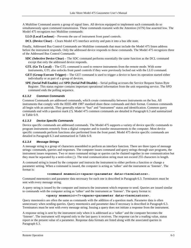
Lake Shore Model 475 Gaussmeter User’s Manual
Remote Operation 6-3
A Multiline Command asserts a group of signal lines. All devices equipped to implement such commands do so simultaneously upon command transmission. These commands transmit with the Attention (ATN) line asserted low. The Model 475 recognizes two Multiline commands:
LLO (Local Lockout) – Prevents the use of instrument front panel controls. DCL (Device Clear) – Clears Model 475 interface activity and puts it into a bus idle state.
Finally, Addressed Bus Control Commands are Multiline commands that must include the Model 475 listen address before the instrument responds. Only the addressed device responds to these commands. The Model 475 recognizes three of the Addressed Bus Control Commands:
SDC (Selective Device Clear) – The SDC command performs essentially the same function as the DCL command except that only the addressed device responds.
GTL (Go To Local) – The GTL command is used to remove instruments from the remote mode. With some instruments, GTL also unlocks front panel controls if they were previously locked out with the LLO command.
GET (Group Execute Trigger) – The GET command is used to trigger a device to have its operation started either individually or as part of a group of devices.
SPE (Serial Poll Enable) and SPD (Serial Poll Disable) – Serial polling accesses the Service Request Status Byte Register. This status register contains important operational information from the unit requesting service. The SPD command ends the polling sequence.
6.1.3.2 Common Commands Common Commands are addressed commands, which create commonality between instruments on the bus. All instruments that comply with the IEEE-488 1987 standard share these commands and their format. Common commands all begin with an asterisk. They generally relate to “bus” and “instrument” status and identification. Common query commands end with a question mark (?). Model 475 common commands are detailed in Paragraph 6.3 and summarized in Table 6-9.
6.1.3.3 Device Specific Commands Device specific commands are addressed commands. The Model 475 supports a variety of device specific commands to program instruments remotely from a digital computer and to transfer measurements to the computer. Most device specific commands perform functions also performed from the front panel. Model 475 device specific commands are detailed in Paragraph 6.3 and summarized in Table 6-9.
6.1.3.4 Message Strings A message string is a group of characters assembled to perform an interface function. There are three types of message strings: commands, queries and responses. The computer issues command and query strings through user programs, the instrument issues responses. Two or more command strings or queries can be chained together in one communication but they must be separated by a semi-colon (;). The total communication string must not exceed 255 characters in length.
A command string is issued by the computer and instructs the instrument to either perform a function or change a parameter setting. When a command is issued, the computer is acting as ‘talker’ and the instrument as ‘listener’. The format is:
<command mnemonic><space><parameter data><terminators>.
Command mnemonics and parameter data necessary for each one is described in Paragraph 6.3. Terminators must be sent with every message string.
A query string is issued by the computer and instructs the instrument which response to send. Queries are issued similar to commands with the computer acting as ‘talker’ and the instrument as ‘listener’. The query format is:
<query mnemonic><?><space><parameter data><terminators>.
Query mnemonics are often the same as commands with the addition of a question mark. Parameter data is often unnecessary when sending queries. Query mnemonics and parameter data if necessary is described in Paragraph 6.3. Terminators must be sent with every message string. Issuing a query does not initiate a response from the instrument.
A response string is sent by the instrument only when it is addressed as a ‘talker’ and the computer becomes the ‘listener’. The instrument will respond only to the last query it receives. The response can be a reading value, status report or the present value of a parameter. Response data formats are listed along with the associated queries in Paragraph 6.3.
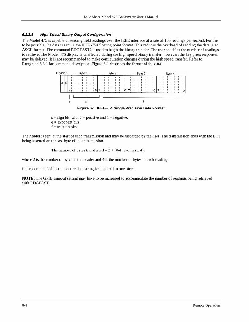
Lake Shore Model 475 Gaussmeter User’s Manual
6-4 Remote Operation
6.1.3.5 High Speed Binary Output Configuration The Model 475 is capable of sending field readings over the IEEE interface at a rate of 100 readings per second. For this to be possible, the data is sent in the IEEE-754 floating point format. This reduces the overhead of sending the data in an ASCII format. The command RDGFAST? is used to begin the binary transfer. The user specifies the number of readings to retrieve. The Model 475 display is unaffected during the high speed binary transfer, however, the key press responses may be delayed. It is not recommended to make configuration changes during the high speed transfer. Refer to Paragraph 6.3.1 for command description. Figure 6-1 describes the format of the data.
Figure 6-1. IEEE-754 Single Precision Data Format
s = sign bit, with 0 = positive and 1 = negative. e = exponent bits f = fraction bits
The header is sent at the start of each transmission and may be discarded by the user. The transmission ends with the EOI being asserted on the last byte of the transmission.
The number of bytes transferred = 2 + (#of readings x 4), where 2 is the number of bytes in the header and 4 is the number of bytes in each reading. It is recommended that the entire data string be acquired in one piece. NOTE: The GPIB timeout setting may have to be increased to accommodate the number of readings being retrieved with RDGFAST.
Lake Shore Model 475 Gaussmeter User’s Manual
Remote Operation 6-5
6.1.4 Status System
6.1.4.1 Overview The Model 475 implements a status system compliant to the IEEE 488.2 – 1992 standard. The status system provides a method of recording and reporting instrument information and is typically used to control the Service Request (SRQ) interrupt line. A diagram of the status system is shown in Figure 6-2. The status system is made up of register sets, the Status Byte register, and the Service Request Enable register. Each register set consists of three types of registers, condition, event, and enable.
6.1.4.1.0 Condition Registers Each register set (except the Standard Event Register set) includes a condition register as shown in Figure 6-2. The condition register constantly monitors the instrument status. The data bits are real-time and are not latched or buffered. The register is read-only.
6.1.4.1.1 Event Registers
Each register set includes an event register as shown in Figure 6-2. Bits in the event register correspond to various system events and latch when the event occurs. When an event bit is set, subsequent events corresponding to that bit are ignored. Set bits remain latched until the register is cleared by a query command (such as *ESR?) or a *CLS command. The register is read-only.
6.1.4.1.2 Enable Registers Each register set includes an enable register as shown in Figure 6-2. An enable register determines which bits in the corresponding event register will set the summary bit for the register set in the Status Byte. The user may write to or read from an enable register. Each event register bit is logically ANDed to the corresponding enable bit of the enable register. When an enable register bit is set by the user, and the corresponding bit is set in the event register, the output (summary) of the register will be set, which in turn sets the summary bit of the Status Byte register.
6.1.4.1.3 Status Byte Register
The Status Byte register, typically referred to as simply the Status Byte, is a non-latching, read-only register that contains all of the summary bits from the register sets. The status of the summary bits are controlled from the register sets as explained above. The Status Byte also contains the Request for Service (RQS)/Master Summary Status (MSS) bit. This bit is used to control the Service Request hardware line on the bus and to report if any of the summary bits are set via the *STB? command. The status of the RQS/MSS bit is controlled by the summary bits and the Service Request Enable Register.
6.1.4.1.4 Service Request Enable Register The Service Request Enable Register determines which summary bits in the Status Byte will set the RQS/MSS bit of the Status Byte. The user may write to or read from the Service Request Enable Register. Each Status Byte summary bit is logically ANDed to the corresponding enable bit of the Service Request Enable Register. When a Service Request enable register bit is set by the user, and the corresponding summary bit is set in the Status Byte, the RQS/MSS bit of the Status Byte will be set, which in turn sets the Service Request hardware line on the bus.
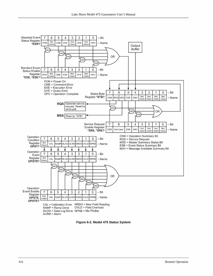
Lake Shore Model 475 Gaussmeter User’s Manual
6-6 Remote Operation
Figure 6-2. Model 475 Status System
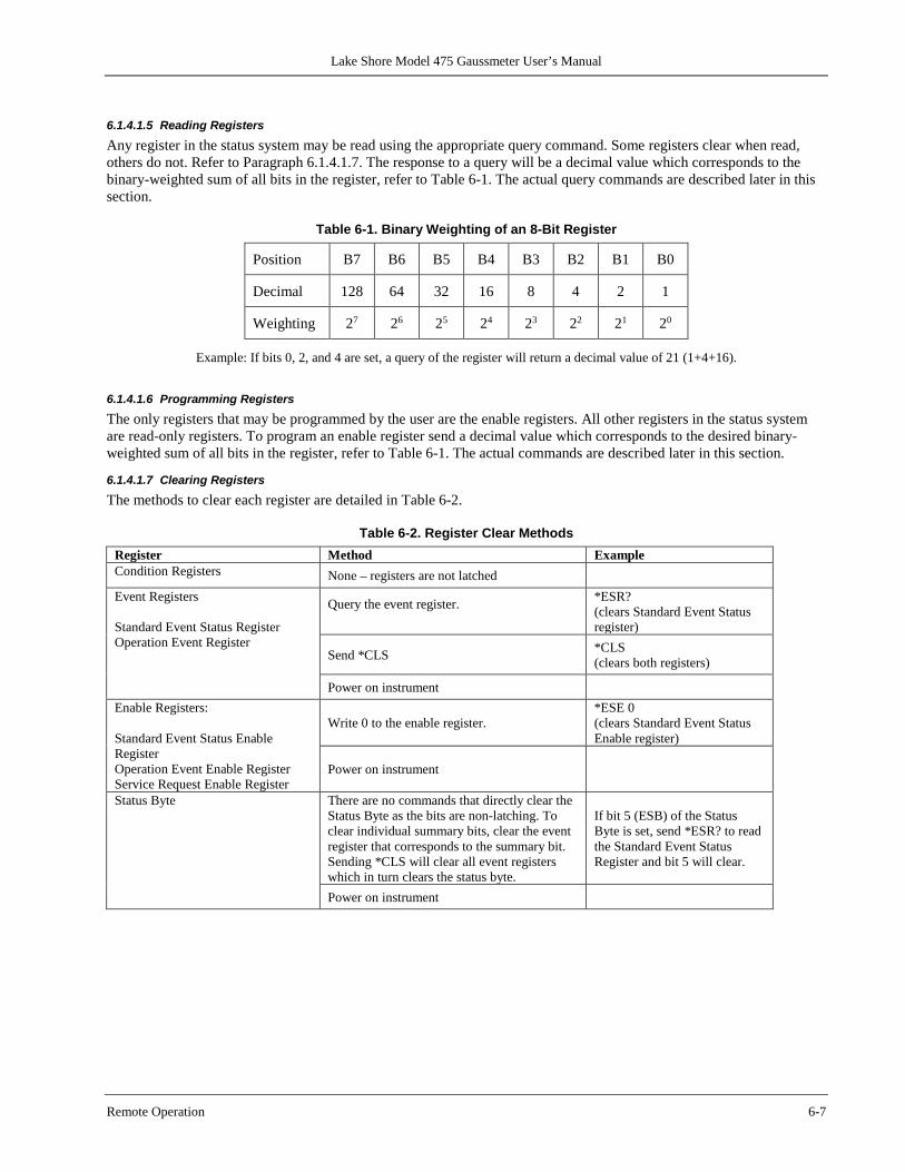
Lake Shore Model 475 Gaussmeter User’s Manual
Remote Operation 6-7
6.1.4.1.5 Reading Registers Any register in the status system may be read using the appropriate query command. Some registers clear when read, others do not. Refer to Paragraph 6.1.4.1.7. The response to a query will be a decimal value which corresponds to the binary-weighted sum of all bits in the register, refer to Table 6-1. The actual query commands are described later in this section.
Table 6-1. Binary Weighting of an 8-Bit Register
Position B7 B6 B5 B4 B3 B2 B1 B0
Decimal 128 64 32 16 8 4 2 1
Weighting 27 26 25 24 23 22 21 20
Example: If bits 0, 2, and 4 are set, a query of the register will return a decimal value of 21 (1+4+16).
6.1.4.1.6 Programming Registers The only registers that may be programmed by the user are the enable registers. All other registers in the status system are read-only registers. To program an enable register send a decimal value which corresponds to the desired binary-weighted sum of all bits in the register, refer to Table 6-1. The actual commands are described later in this section.
6.1.4.1.7 Clearing Registers The methods to clear each register are detailed in Table 6-2.
Table 6-2. Register Clear Methods Register Method Example Condition Registers None – registers are not latched Event Registers Standard Event Status Register Operation Event Register
Query the event register.
*ESR? (clears Standard Event Status register)
Send *CLS *CLS (clears both registers)
Power on instrument Enable Registers: Standard Event Status Enable Register Operation Event Enable Register Service Request Enable Register
Write 0 to the enable register. *ESE 0 (clears Standard Event Status Enable register)
Power on instrument
Status Byte There are no commands that directly clear the Status Byte as the bits are non-latching. To clear individual summary bits, clear the event register that corresponds to the summary bit. Sending *CLS will clear all event registers which in turn clears the status byte.
If bit 5 (ESB) of the Status Byte is set, send *ESR? to read the Standard Event Status Register and bit 5 will clear.
Power on instrument
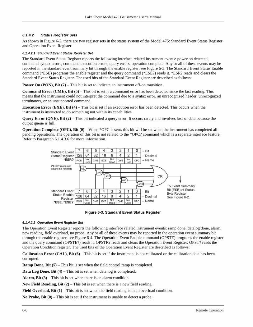
Lake Shore Model 475 Gaussmeter User’s Manual
6-8 Remote Operation
6.1.4.2 Status Register Sets As shown in Figure 6-2, there are two register sets in the status system of the Model 475: Standard Event Status Register and Operation Event Register.
6.1.4.2.1 Standard Event Status Register Set The Standard Event Status Register reports the following interface related instrument events: power on detected, command syntax errors, command execution errors, query errors, operation complete. Any or all of these events may be reported in the standard event summary bit through the enable register, see Figure 6-3. The Standard Event Status Enable command (*ESE) programs the enable register and the query command (*ESE?) reads it. *ESR? reads and clears the Standard Event Status Register. The used bits of the Standard Event Register are described as follows:
Power On (PON), Bit (7) – This bit is set to indicate an instrument off-on transition. Command Error (CME), Bit (5) – This bit is set if a command error has been detected since the last reading. This means that the instrument could not interpret the command due to a syntax error, an unrecognized header, unrecognized terminators, or an unsupported command. Execution Error (EXE), Bit (4) – This bit is set if an execution error has been detected. This occurs when the instrument is instructed to do something not within its capabilities. Query Error (QYE), Bit (2) – This bit indicated a query error. It occurs rarely and involves loss of data because the output queue is full. Operation Complete (OPC), Bit (0) – When *OPC is sent, this bit will be set when the instrument has completed all pending operations. The operation of this bit is not related to the *OPC? command which is a separate interface feature. Refer to Paragraph 6.1.4.3.6 for more information.
Figure 6-3. Standard Event Status Register
6.1.4.2.2 Operation Event Register Set The Operation Event Register reports the following interface related instrument events: ramp done, datalog done, alarm, new reading, field overload, no probe. Any or all of these events may be reported in the operation event summary bit through the enable register, see Figure 6-4. The Operation Event Enable command (OPSTE) programs the enable register and the query command (OPSTE?) reads it. OPSTR? reads and clears the Operation Event Register. OPST? reads the Operation Condition register. The used bits of the Operation Event Register are described as follows:
Calibration Error (CAL), Bit (6) – This bit is set if the instrument is not calibrated or the calibration data has been corrupted. Ramp Done, Bit (5) – This bit is set when the field control ramp is completed. Data Log Done, Bit (4) – This bit is set when data log is completed. Alarm, Bit (3) – This bit is set when there is an alarm condition. New Field Reading, Bit (2) – This bit is set when there is a new field reading. Field Overload, Bit (1) – This bit is set when the field reading is in an overload condition. No Probe, Bit (0) – This bit is set if the instrument is unable to detect a probe.
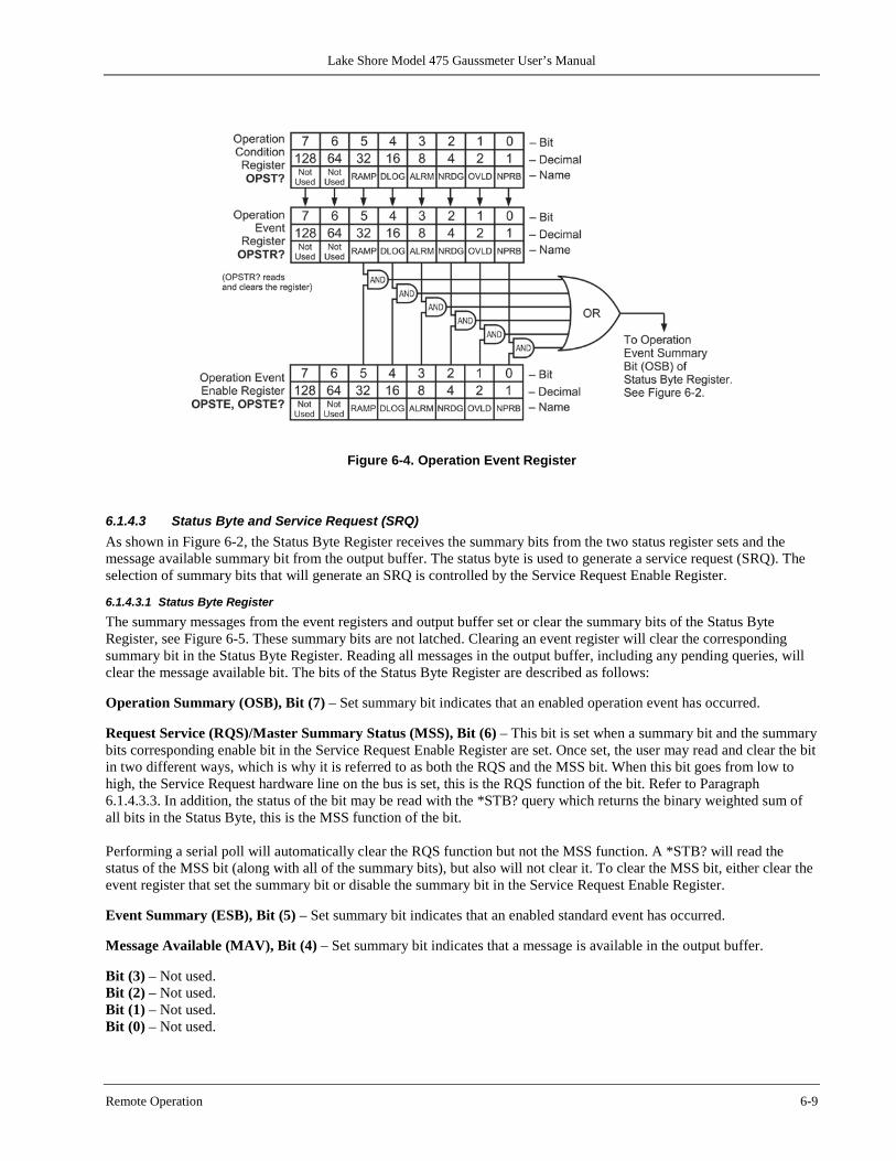
Lake Shore Model 475 Gaussmeter User’s Manual
Remote Operation 6-9
Figure 6-4. Operation Event Register
6.1.4.3 Status Byte and Service Request (SRQ) As shown in Figure 6-2, the Status Byte Register receives the summary bits from the two status register sets and the message available summary bit from the output buffer. The status byte is used to generate a service request (SRQ). The selection of summary bits that will generate an SRQ is controlled by the Service Request Enable Register.
6.1.4.3.1 Status Byte Register The summary messages from the event registers and output buffer set or clear the summary bits of the Status Byte Register, see Figure 6-5. These summary bits are not latched. Clearing an event register will clear the corresponding summary bit in the Status Byte Register. Reading all messages in the output buffer, including any pending queries, will clear the message available bit. The bits of the Status Byte Register are described as follows: Operation Summary (OSB), Bit (7) – Set summary bit indicates that an enabled operation event has occurred. Request Service (RQS)/Master Summary Status (MSS), Bit (6) – This bit is set when a summary bit and the summary bits corresponding enable bit in the Service Request Enable Register are set. Once set, the user may read and clear the bit in two different ways, which is why it is referred to as both the RQS and the MSS bit. When this bit goes from low to high, the Service Request hardware line on the bus is set, this is the RQS function of the bit. Refer to Paragraph 6.1.4.3.3. In addition, the status of the bit may be read with the *STB? query which returns the binary weighted sum of all bits in the Status Byte, this is the MSS function of the bit. Performing a serial poll will automatically clear the RQS function but not the MSS function. A *STB? will read the status of the MSS bit (along with all of the summary bits), but also will not clear it. To clear the MSS bit, either clear the event register that set the summary bit or disable the summary bit in the Service Request Enable Register. Event Summary (ESB), Bit (5) – Set summary bit indicates that an enabled standard event has occurred. Message Available (MAV), Bit (4) – Set summary bit indicates that a message is available in the output buffer. Bit (3) – Not used. Bit (2) – Not used. Bit (1) – Not used. Bit (0) – Not used.
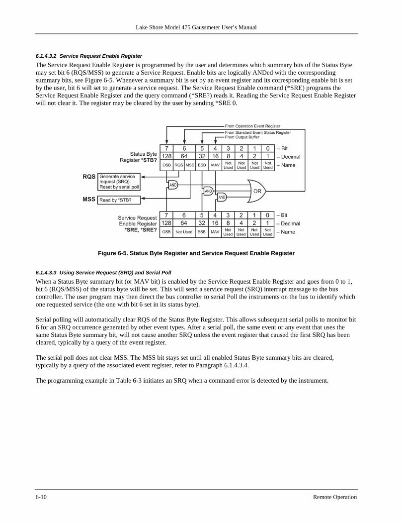
Lake Shore Model 475 Gaussmeter User’s Manual
6-10 Remote Operation
6.1.4.3.2 Service Request Enable Register The Service Request Enable Register is programmed by the user and determines which summary bits of the Status Byte may set bit 6 (RQS/MSS) to generate a Service Request. Enable bits are logically ANDed with the corresponding summary bits, see Figure 6-5. Whenever a summary bit is set by an event register and its corresponding enable bit is set by the user, bit 6 will set to generate a service request. The Service Request Enable command (*SRE) programs the Service Request Enable Register and the query command (*SRE?) reads it. Reading the Service Request Enable Register will not clear it. The register may be cleared by the user by sending *SRE 0.
Figure 6-5. Status Byte Register and Service Request Enable Register
6.1.4.3.3 Using Service Request (SRQ) and Serial Poll When a Status Byte summary bit (or MAV bit) is enabled by the Service Request Enable Register and goes from 0 to 1, bit 6 (RQS/MSS) of the status byte will be set. This will send a service request (SRQ) interrupt message to the bus controller. The user program may then direct the bus controller to serial Poll the instruments on the bus to identify which one requested service (the one with bit 6 set in its status byte). Serial polling will automatically clear RQS of the Status Byte Register. This allows subsequent serial polls to monitor bit 6 for an SRQ occurrence generated by other event types. After a serial poll, the same event or any event that uses the same Status Byte summary bit, will not cause another SRQ unless the event register that caused the first SRQ has been cleared, typically by a query of the event register. The serial poll does not clear MSS. The MSS bit stays set until all enabled Status Byte summary bits are cleared, typically by a query of the associated event register, refer to Paragraph 6.1.4.3.4. The programming example in Table 6-3 initiates an SRQ when a command error is detected by the instrument.
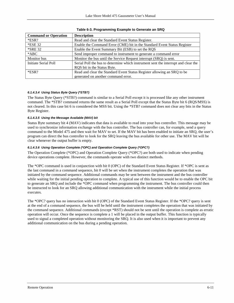
Lake Shore Model 475 Gaussmeter User’s Manual
Remote Operation 6-11
Table 6-3. Programming Example to Generate an SRQ Command or Operation Description *ESR? Read and clear the Standard Event Status Register. *ESE 32 Enable the Command Error (CME) bit in the Standard Event Status Register *SRE 32 Enable the Event Summary Bit (ESB) to set the RQS *ABC Send improper command to instrument to generate a command error Monitor bus Monitor the bus until the Service Request interrupt (SRQ) is sent. Initiate Serial Poll Serial Poll the bus to determine which instrument sent the interrupt and clear the
RQS bit in the Status Byte. *ESR? Read and clear the Standard Event Status Register allowing an SRQ to be
generated on another command error.
6.1.4.3.4 Using Status Byte Query (*STB?) The Status Byte Query (*STB?) command is similar to a Serial Poll except it is processed like any other instrument command. The *STB? command returns the same result as a Serial Poll except that the Status Byte bit 6 (RQS/MSS) is not cleared. In this case bit 6 is considered the MSS bit. Using the *STB? command does not clear any bits in the Status Byte Register.
6.1.4.3.5 Using the Message Available (MAV) bit Status Byte summary bit 4 (MAV) indicates that data is available to read into your bus controller. This message may be used to synchronize information exchange with the bus controller. The bus controller can, for example, send a query command to the Model 475 and then wait for MAV to set. If the MAV bit has been enabled to initiate an SRQ, the user’s program can direct the bus controller to look for the SRQ leaving the bus available for other use. The MAV bit will be clear whenever the output buffer is empty.
6.1.4.3.6 Using Operation Complete (*OPC) and Operation Complete Query (*OPC?) The Operation Complete (*OPC) and Operation Complete Query (*OPC?) are both used to indicate when pending device operations complete. However, the commands operate with two distinct methods. The *OPC command is used in conjunction with bit 0 (OPC) of the Standard Event Status Register. If *OPC is sent as the last command in a command sequence, bit 0 will be set when the instrument completes the operation that was initiated by the command sequence. Additional commands may be sent between the instrument and the bus controller while waiting for the initial pending operation to complete. A typical use of this function would be to enable the OPC bit to generate an SRQ and include the *OPC command when programming the instrument. The bus controller could then be instructed to look for an SRQ allowing additional communication with the instrument while the initial process executes. The *OPC? query has no interaction with bit 0 (OPC) of the Standard Event Status Register. If the *OPC? query is sent at the end of a command sequence, the bus will be held until the instrument completes the operation that was initiated by the command sequence. Additional commands (except *RST) should not be sent until the operation is complete as erratic operation will occur. Once the sequence is complete a 1 will be placed in the output buffer. This function is typically used to signal a completed operation without monitoring the SRQ. It is also used when it is important to prevent any additional communication on the bus during a pending operation.
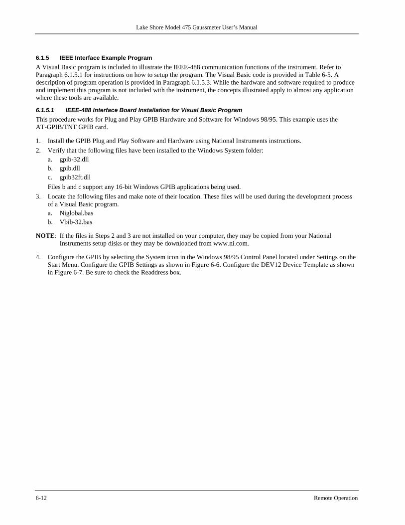
Lake Shore Model 475 Gaussmeter User’s Manual
6-12 Remote Operation
6.1.5 IEEE Interface Example Program A Visual Basic program is included to illustrate the IEEE-488 communication functions of the instrument. Refer to Paragraph 6.1.5.1 for instructions on how to setup the program. The Visual Basic code is provided in Table 6-5. A description of program operation is provided in Paragraph 6.1.5.3. While the hardware and software required to produce and implement this program is not included with the instrument, the concepts illustrated apply to almost any application where these tools are available.
6.1.5.1 IEEE-488 Interface Board Installation for Visual Basic Program This procedure works for Plug and Play GPIB Hardware and Software for Windows 98/95. This example uses the AT-GPIB/TNT GPIB card. 1. Install the GPIB Plug and Play Software and Hardware using National Instruments instructions. 2. Verify that the following files have been installed to the Windows System folder:
a. gpib-32.dll b. gpib.dll c. gpib32ft.dll Files b and c support any 16-bit Windows GPIB applications being used.
3. Locate the following files and make note of their location. These files will be used during the development process of a Visual Basic program. a. Niglobal.bas b. Vbib-32.bas
NOTE: If the files in Steps 2 and 3 are not installed on your computer, they may be copied from your National
Instruments setup disks or they may be downloaded from www.ni.com. 4. Configure the GPIB by selecting the System icon in the Windows 98/95 Control Panel located under Settings on the
Start Menu. Configure the GPIB Settings as shown in Figure 6-6. Configure the DEV12 Device Template as shown in Figure 6-7. Be sure to check the Readdress box.
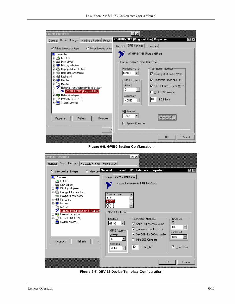
Lake Shore Model 475 Gaussmeter User’s Manual
Remote Operation 6-13
Figure 6-6. GPIB0 Setting Configuration
Figure 6-7. DEV 12 Device Template Configuration
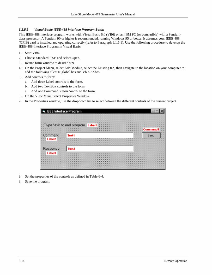
Lake Shore Model 475 Gaussmeter User’s Manual
6-14 Remote Operation
6.1.5.2 Visual Basic IEEE-488 Interface Program Setup This IEEE-488 interface program works with Visual Basic 6.0 (VB6) on an IBM PC (or compatible) with a Pentium-class processor. A Pentium 90 or higher is recommended, running Windows 95 or better. It assumes your IEEE-488 (GPIB) card is installed and operating correctly (refer to Paragraph 6.1.5.1). Use the following procedure to develop the IEEE-488 Interface Program in Visual Basic.
1. Start VB6. 2. Choose Standard EXE and select Open. 3. Resize form window to desired size. 4. On the Project Menu, select Add Module, select the Existing tab, then navigate to the location on your computer to
add the following files: Niglobal.bas and Vbib-32.bas. 5. Add controls to form:
a. Add three Label controls to the form. b. Add two TextBox controls to the form. c. Add one CommandButton control to the form.
6. On the View Menu, select Properties Window. 7. In the Properties window, use the dropdown list to select between the different controls of the current project.
8. Set the properties of the controls as defined in Table 6-4. 9. Save the program.
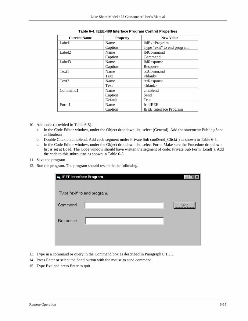
Lake Shore Model 475 Gaussmeter User’s Manual
Remote Operation 6-15
Table 6-4. IEEE-488 Interface Program Control Properties Current Name Property New Value
Label1 Name Caption
lblExitProgram Type “exit” to end program.
Label2 Name Caption
lblCommand Command
Label3 Name Caption
lblResponse Response
Text1 Name Text
txtCommand <blank>
Text2 Name Text
txtResponse <blank>
Command1 Name Caption Default
cmdSend Send True
Form1 Name Caption
frmIEEE IEEE Interface Program
10. Add code (provided in Table 6-5).
a. In the Code Editor window, under the Object dropdown list, select (General). Add the statement: Public gSend as Boolean
b. Double Click on cmdSend. Add code segment under Private Sub cmdSend_Click( ) as shown in Table 6-5. c. In the Code Editor window, under the Object dropdown list, select Form. Make sure the Procedure dropdown
list is set at Load. The Code window should have written the segment of code: Private Sub Form_Load( ). Add the code to this subroutine as shown in Table 6-5.
11. Save the program. 12. Run the program. The program should resemble the following.
13. Type in a command or query in the Command box as described in Paragraph 6.1.5.5. 14. Press Enter or select the Send button with the mouse to send command. 15. Type Exit and press Enter to quit.

Lake Shore Model 475 Gaussmeter User’s Manual
6-16 Remote Operation
Table 6-5. Visual Basic IEEE-488 Interface Program Public gSend As Boolean 'Global used for Send button state Private Sub cmdSend_Click() 'Routine to handle Send button press gSend = True 'Set Flag to True End Sub Private Sub Form_Load() 'Main code section Dim strReturn As String 'Used to return response Dim term As String 'Terminators Dim strCommand As String 'Data string sent to instrument Dim intDevice As Integer 'Device number used with IEEE frmIEEE.Show 'Show main window term = Chr(13) & Chr(10) 'Terminators are <CR><LF> strReturn = "" 'Clear return string Call ibdev(0, 12, 0, T10s, 1, &H140A, intDevice) 'Initialize the IEEE device Call ibconfig(intDevice, ibcREADDR,1) 'Setup Repeat Addressing Do Do 'Wait loop DoEvents 'Give up processor to other events Loop Until gSend = True 'Loop until Send button pressed gSend = False 'Set Flag as False strCommand = frmIEEE.txtCommand.Text 'Get Command strReturn = "" 'Clear response display strCommand = UCase(strCommand) 'Set all characters to upper case If strCommand = "EXIT" Then 'Get out on EXIT End End If Call ibwrt(intDevice, strCommand & term) 'Send command to instrument If (ibsta And EERR) Then 'Check for IEEE errors 'do error handling if needed 'Handle errors here End If If InStr(strCommand, "?") <> 0 Then 'Check to see if query strReturn = Space(100) 'Build empty return buffer Call ibrd(intDevice, strReturn) 'Read back response If (ibsta And EERR) Then 'Check for IEEE errors 'do error handling if needed 'Handle errors here End If If strReturn <> "" Then 'Check if empty string strReturn = RTrim(strReturn) 'Remove extra spaces and Terminators Do While Right(strReturn, 1) = Chr(10) Or Right(strReturn, 1) = Chr(13) strReturn = Left(strReturn, Len(strReturn) - 1) Loop Else strReturn = "No Response" 'Send No Response End If frmIEEE.txtResponse.Text = strReturn 'Put response in text on main form End If Loop End Sub
Lake Shore Model 475 Gaussmeter User’s Manual
Remote Operation 6-17
6.1.5.3 Program Operation Once either example program is running, try the following commands and observe the response of the instrument. Input from the user is shown in bold and terminators are added by the program. The word [term] indicates the required terminators included with the response. ENTER COMMAND? *IDN? Identification query. Instrument will return a string identifying itself. RESPONSE: LSCI,MODEL475,1234567,02032003[term] ENTER COMMAND? RDGFIELD? Field reading query. Instrument will return a string with the present
field reading in the present units. RESPONSE: +273.150E+00[term] ENTER COMMAND? RANGE 1 Field range command. Instrument will set to the lowest range. No
response will be sent. ENTER COMMAND? RANGE? Field range query. Instrument will return a string with the present field
range setting. RESPONSE: 1[term] ENTER COMMAND? RANGE 5;RANGE? Field range command followed by a query. Instrument will change to
the highest range setting then return a string RESPONSE: 5[term] with the present setting.
The following are additional notes on using either IEEE-488 Interface program. • If you enter a correctly spelled query without a “?,” nothing will be returned. Incorrectly spelled commands and
queries are ignored. Commands and queries should have a space separating the command and associated parameters. • Leading zeros and zeros following a decimal point are not needed in a command string, but are sent in response to a
query. A leading “+” is not required but a leading “–” is required.
6.1.6 Troubleshooting New Installation 1. Check instrument address. 2. Always send terminators. 3. Send entire message string at one time including terminators. 4. Send only one simple command at a time until communication is established. 5. Be sure to spell commands correctly and use proper syntax. 6. Attempt both ‘Talk’ and ‘Listen’ functions. If one works but not the other, the hardware connection is working, so
look at syntax, terminators, and command format. 7. If only one message is received after resetting the interface, check the “repeat addressing” setting. It should be
enabled. Old Installation No Longer Working 8. Power instrument off then on again to see if it is a soft failure. 9. Power computer off then on again to see if the IEEE card is locked up. 10. Verify that the address has not been changed on the instrument during a memory reset. 11. Check all cable connections. Intermittent Lockups 12. Check cable connections and length. 13. Increase delay between all commands to 50 ms to make sure instrument is not being over loaded.
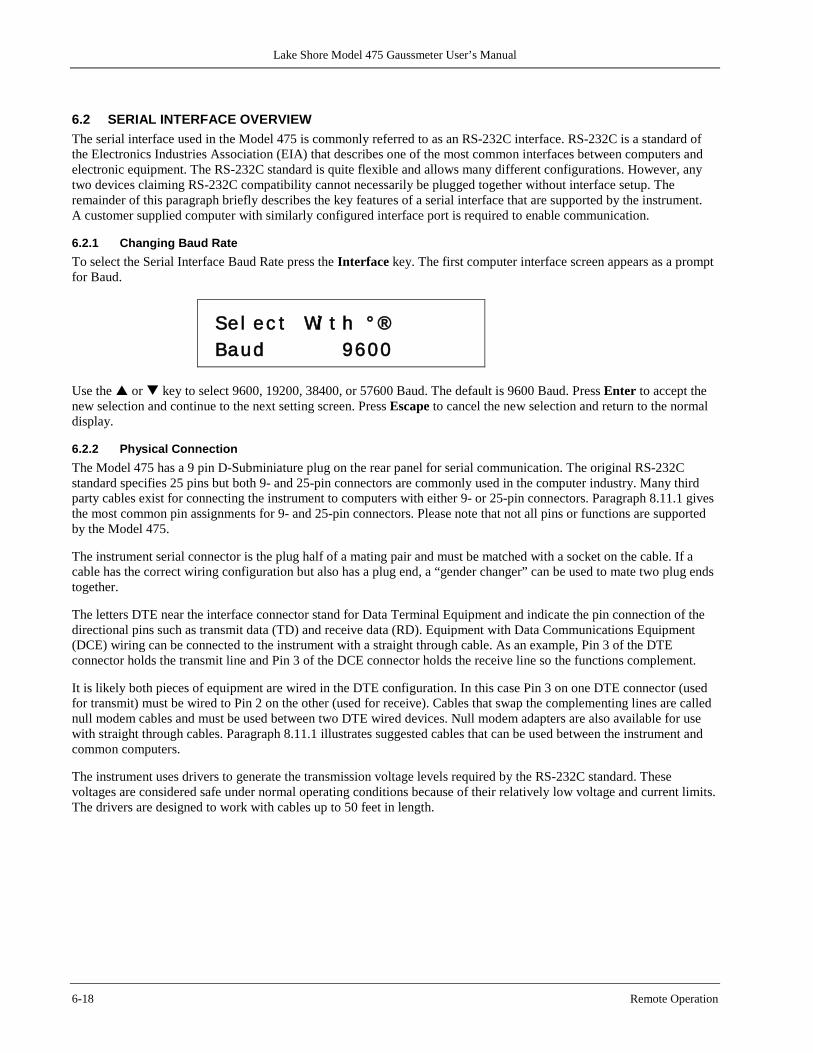
Lake Shore Model 475 Gaussmeter User’s Manual
6-18 Remote Operation
6.2 SERIAL INTERFACE OVERVIEW The serial interface used in the Model 475 is commonly referred to as an RS-232C interface. RS-232C is a standard of the Electronics Industries Association (EIA) that describes one of the most common interfaces between computers and electronic equipment. The RS-232C standard is quite flexible and allows many different configurations. However, any two devices claiming RS-232C compatibility cannot necessarily be plugged together without interface setup. The remainder of this paragraph briefly describes the key features of a serial interface that are supported by the instrument. A customer supplied computer with similarly configured interface port is required to enable communication.
6.2.1 Changing Baud Rate To select the Serial Interface Baud Rate press the Interface key. The first computer interface screen appears as a prompt for Baud.
Se l ec t Wi t h ° ® Baud 9600
Use the or key to select 9600, 19200, 38400, or 57600 Baud. The default is 9600 Baud. Press Enter to accept the new selection and continue to the next setting screen. Press Escape to cancel the new selection and return to the normal display.
6.2.2 Physical Connection The Model 475 has a 9 pin D-Subminiature plug on the rear panel for serial communication. The original RS-232C standard specifies 25 pins but both 9- and 25-pin connectors are commonly used in the computer industry. Many third party cables exist for connecting the instrument to computers with either 9- or 25-pin connectors. Paragraph 8.11.1 gives the most common pin assignments for 9- and 25-pin connectors. Please note that not all pins or functions are supported by the Model 475. The instrument serial connector is the plug half of a mating pair and must be matched with a socket on the cable. If a cable has the correct wiring configuration but also has a plug end, a “gender changer” can be used to mate two plug ends together. The letters DTE near the interface connector stand for Data Terminal Equipment and indicate the pin connection of the directional pins such as transmit data (TD) and receive data (RD). Equipment with Data Communications Equipment (DCE) wiring can be connected to the instrument with a straight through cable. As an example, Pin 3 of the DTE connector holds the transmit line and Pin 3 of the DCE connector holds the receive line so the functions complement. It is likely both pieces of equipment are wired in the DTE configuration. In this case Pin 3 on one DTE connector (used for transmit) must be wired to Pin 2 on the other (used for receive). Cables that swap the complementing lines are called null modem cables and must be used between two DTE wired devices. Null modem adapters are also available for use with straight through cables. Paragraph 8.11.1 illustrates suggested cables that can be used between the instrument and common computers. The instrument uses drivers to generate the transmission voltage levels required by the RS-232C standard. These voltages are considered safe under normal operating conditions because of their relatively low voltage and current limits. The drivers are designed to work with cables up to 50 feet in length.
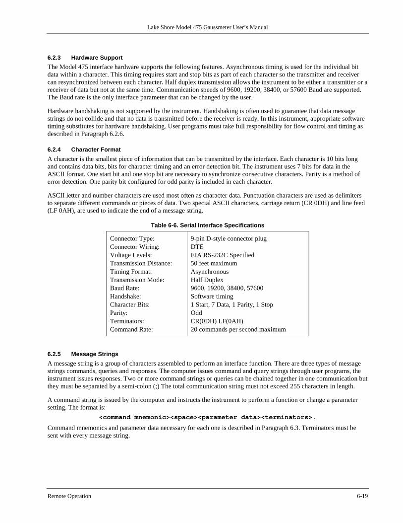
Lake Shore Model 475 Gaussmeter User’s Manual
Remote Operation 6-19
6.2.3 Hardware Support The Model 475 interface hardware supports the following features. Asynchronous timing is used for the individual bit data within a character. This timing requires start and stop bits as part of each character so the transmitter and receiver can resynchronized between each character. Half duplex transmission allows the instrument to be either a transmitter or a receiver of data but not at the same time. Communication speeds of 9600, 19200, 38400, or 57600 Baud are supported. The Baud rate is the only interface parameter that can be changed by the user. Hardware handshaking is not supported by the instrument. Handshaking is often used to guarantee that data message strings do not collide and that no data is transmitted before the receiver is ready. In this instrument, appropriate software timing substitutes for hardware handshaking. User programs must take full responsibility for flow control and timing as described in Paragraph 6.2.6.
6.2.4 Character Format A character is the smallest piece of information that can be transmitted by the interface. Each character is 10 bits long and contains data bits, bits for character timing and an error detection bit. The instrument uses 7 bits for data in the ASCII format. One start bit and one stop bit are necessary to synchronize consecutive characters. Parity is a method of error detection. One parity bit configured for odd parity is included in each character. ASCII letter and number characters are used most often as character data. Punctuation characters are used as delimiters to separate different commands or pieces of data. Two special ASCII characters, carriage return (CR 0DH) and line feed (LF 0AH), are used to indicate the end of a message string.
Table 6-6. Serial Interface Specifications
Connector Type: Connector Wiring: Voltage Levels: Transmission Distance: Timing Format: Transmission Mode: Baud Rate: Handshake: Character Bits: Parity: Terminators: Command Rate:
9-pin D-style connector plug DTE EIA RS-232C Specified 50 feet maximum Asynchronous Half Duplex 9600, 19200, 38400, 57600 Software timing 1 Start, 7 Data, 1 Parity, 1 Stop Odd CR(0DH) LF(0AH) 20 commands per second maximum
6.2.5 Message Strings A message string is a group of characters assembled to perform an interface function. There are three types of message strings commands, queries and responses. The computer issues command and query strings through user programs, the instrument issues responses. Two or more command strings or queries can be chained together in one communication but they must be separated by a semi-colon (;) The total communication string must not exceed 255 characters in length. A command string is issued by the computer and instructs the instrument to perform a function or change a parameter setting. The format is:
<command mnemonic><space><parameter data><terminators>.
Command mnemonics and parameter data necessary for each one is described in Paragraph 6.3. Terminators must be sent with every message string.
Lake Shore Model 475 Gaussmeter User’s Manual
6-20 Remote Operation
Message Strings (Continued)
A query string is issued by the computer and instructs the instrument to send a response. The query format is: <query mnemonic><?><space><parameter data><terminators>.
Query mnemonics are often the same as commands with the addition of a question mark. Parameter data is often unnecessary when sending queries. Query mnemonics and parameter data if necessary is described in Paragraph 6.3. Terminators must be sent with every message string. The computer should expect a response very soon after a query is sent. A response string is the instruments response or answer to a query string. The instrument will respond only to the last query it receives. The response can be a reading value, status report or the present value of a parameter. Response data formats are listed along with the associated queries in Paragraph 6.3. The response is sent as soon as possible after the instrument receives the query. Typically, it takes 10 ms for the instrument to begin the response. Some responses take longer.
6.2.6 Message Flow Control It is important to remember that the user program is in charge of the serial communication at all times. The instrument can not initiate communication, determine which device should be transmitting at a given time or guarantee timing between messages. All of this is the responsibility of the user program. When issuing commands only the user program should: • Properly format and transmit the command including terminators as one string. • Guarantee that no other communication is started for 50 ms after the last character is transmitted. • Not initiate communication more than 20 times per second. When issuing queries or queries and commands together the user program should: • Properly format and transmit the query including terminators as one string. • Prepare to receive a response immediately. • Receive the entire response from the instrument including the terminators. • Guarantee that no other communication is started during the response or for 50 ms after it completes. • Not initiate communication more than 20 times per second. Failure to follow these simple rules will result in inability to establish communication with the instrument or intermittent failures in communication.
6.2.7 Serial Interface Example Program A Visual Basic program is included to illustrate the serial communication functions of the instrument. Refer to Paragraph 6.2.7.1 for instructions on how to setup the program. The Visual Basic code is provided in Table 6-8. A description of program operation is provided in Paragraph 6.2.7.2. While the hardware and software required to produce and implement this program is not included with the instrument, the concepts illustrated apply to almost any application where these tools are available.
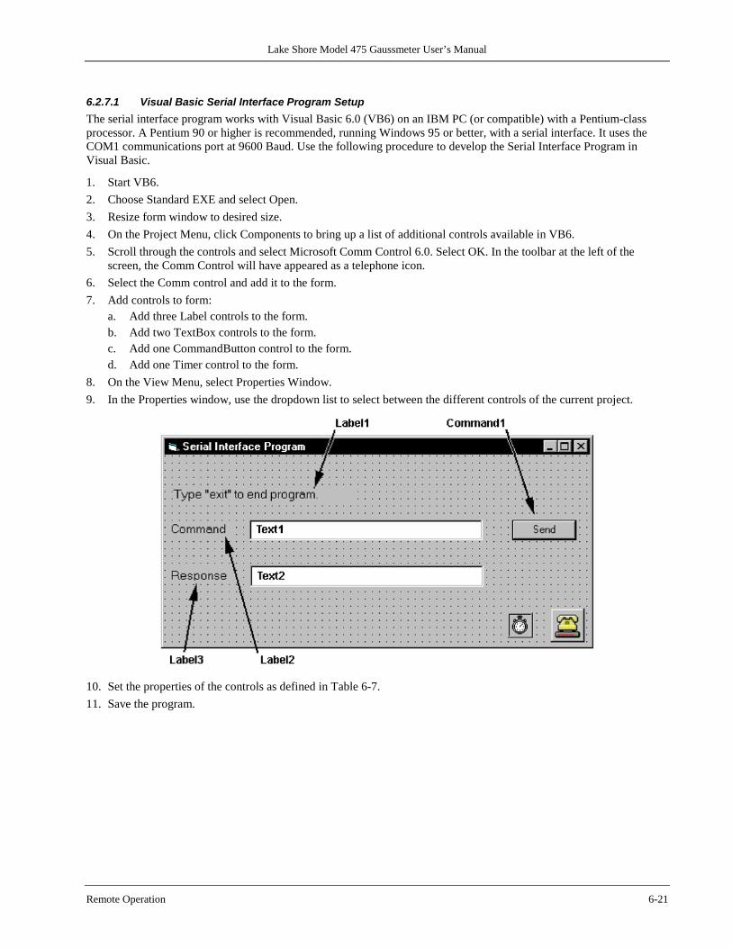
Lake Shore Model 475 Gaussmeter User’s Manual
Remote Operation 6-21
6.2.7.1 Visual Basic Serial Interface Program Setup The serial interface program works with Visual Basic 6.0 (VB6) on an IBM PC (or compatible) with a Pentium-class processor. A Pentium 90 or higher is recommended, running Windows 95 or better, with a serial interface. It uses the COM1 communications port at 9600 Baud. Use the following procedure to develop the Serial Interface Program in Visual Basic.
1. Start VB6. 2. Choose Standard EXE and select Open. 3. Resize form window to desired size. 4. On the Project Menu, click Components to bring up a list of additional controls available in VB6. 5. Scroll through the controls and select Microsoft Comm Control 6.0. Select OK. In the toolbar at the left of the
screen, the Comm Control will have appeared as a telephone icon. 6. Select the Comm control and add it to the form. 7. Add controls to form:
a. Add three Label controls to the form. b. Add two TextBox controls to the form. c. Add one CommandButton control to the form. d. Add one Timer control to the form.
8. On the View Menu, select Properties Window. 9. In the Properties window, use the dropdown list to select between the different controls of the current project.
10. Set the properties of the controls as defined in Table 6-7. 11. Save the program.
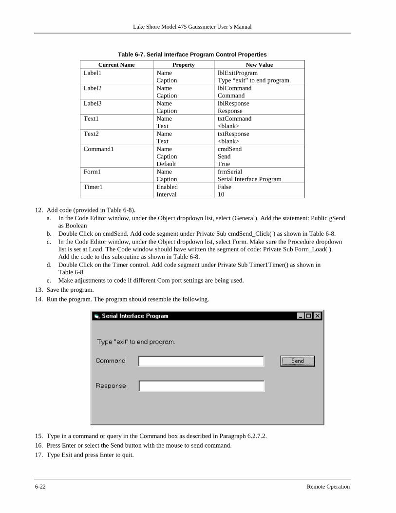
Lake Shore Model 475 Gaussmeter User’s Manual
6-22 Remote Operation
Table 6-7. Serial Interface Program Control Properties
Current Name Property New Value Label1 Name
Caption lblExitProgram Type “exit” to end program.
Label2 Name Caption
lblCommand Command
Label3 Name Caption
lblResponse Response
Text1 Name Text
txtCommand <blank>
Text2 Name Text
txtResponse <blank>
Command1 Name Caption Default
cmdSend Send True
Form1 Name Caption
frmSerial Serial Interface Program
Timer1 Enabled Interval
False 10
12. Add code (provided in Table 6-8). a. In the Code Editor window, under the Object dropdown list, select (General). Add the statement: Public gSend
as Boolean b. Double Click on cmdSend. Add code segment under Private Sub cmdSend_Click( ) as shown in Table 6-8. c. In the Code Editor window, under the Object dropdown list, select Form. Make sure the Procedure dropdown
list is set at Load. The Code window should have written the segment of code: Private Sub Form_Load( ). Add the code to this subroutine as shown in Table 6-8.
d. Double Click on the Timer control. Add code segment under Private Sub Timer1Timer() as shown in Table 6-8.
e. Make adjustments to code if different Com port settings are being used. 13. Save the program. 14. Run the program. The program should resemble the following.
15. Type in a command or query in the Command box as described in Paragraph 6.2.7.2. 16. Press Enter or select the Send button with the mouse to send command. 17. Type Exit and press Enter to quit.
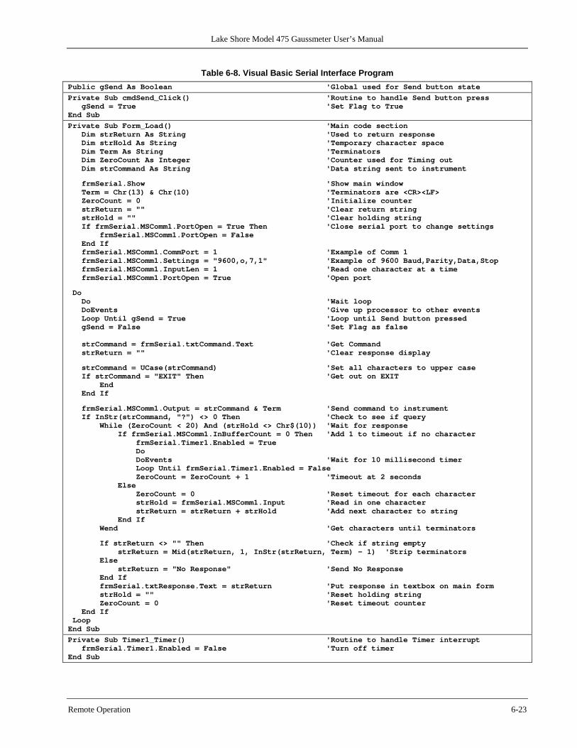
Lake Shore Model 475 Gaussmeter User’s Manual
Remote Operation 6-23
Table 6-8. Visual Basic Serial Interface Program Public gSend As Boolean 'Global used for Send button state
Private Sub cmdSend_Click() 'Routine to handle Send button press gSend = True 'Set Flag to True End Sub
Private Sub Form_Load() 'Main code section Dim strReturn As String 'Used to return response Dim strHold As String 'Temporary character space Dim Term As String 'Terminators Dim ZeroCount As Integer 'Counter used for Timing out Dim strCommand As String 'Data string sent to instrument frmSerial.Show 'Show main window Term = Chr(13) & Chr(10) 'Terminators are <CR><LF> ZeroCount = 0 'Initialize counter strReturn = "" 'Clear return string strHold = "" 'Clear holding string If frmSerial.MSComm1.PortOpen = True Then 'Close serial port to change settings frmSerial.MSComm1.PortOpen = False End If frmSerial.MSComm1.CommPort = 1 'Example of Comm 1 frmSerial.MSComm1.Settings = "9600,o,7,1" 'Example of 9600 Baud,Parity,Data,Stop frmSerial.MSComm1.InputLen = 1 'Read one character at a time frmSerial.MSComm1.PortOpen = True 'Open port Do Do 'Wait loop DoEvents 'Give up processor to other events Loop Until gSend = True 'Loop until Send button pressed gSend = False 'Set Flag as false strCommand = frmSerial.txtCommand.Text 'Get Command strReturn = "" 'Clear response display strCommand = UCase(strCommand) 'Set all characters to upper case If strCommand = "EXIT" Then 'Get out on EXIT End End If frmSerial.MSComm1.Output = strCommand & Term 'Send command to instrument If InStr(strCommand, "?") <> 0 Then 'Check to see if query While (ZeroCount < 20) And (strHold <> Chr$(10)) 'Wait for response If frmSerial.MSComm1.InBufferCount = 0 Then 'Add 1 to timeout if no character frmSerial.Timer1.Enabled = True Do DoEvents 'Wait for 10 millisecond timer Loop Until frmSerial.Timer1.Enabled = False ZeroCount = ZeroCount + 1 'Timeout at 2 seconds Else ZeroCount = 0 'Reset timeout for each character strHold = frmSerial.MSComm1.Input 'Read in one character strReturn = strReturn + strHold 'Add next character to string End If Wend 'Get characters until terminators If strReturn <> "" Then 'Check if string empty strReturn = Mid(strReturn, 1, InStr(strReturn, Term) – 1) 'Strip terminators Else strReturn = "No Response" 'Send No Response End If frmSerial.txtResponse.Text = strReturn 'Put response in textbox on main form strHold = "" 'Reset holding string ZeroCount = 0 'Reset timeout counter End If Loop End Sub
Private Sub Timer1_Timer() 'Routine to handle Timer interrupt frmSerial.Timer1.Enabled = False 'Turn off timer End Sub
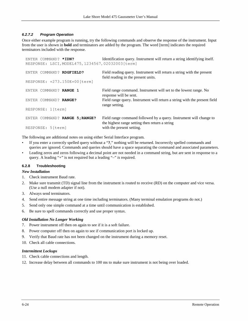
Lake Shore Model 475 Gaussmeter User’s Manual
6-24 Remote Operation
6.2.7.2 Program Operation Once either example program is running, try the following commands and observe the response of the instrument. Input from the user is shown in bold and terminators are added by the program. The word [term] indicates the required terminators included with the response. ENTER COMMAND? *IDN? Identification query. Instrument will return a string identifying itself. RESPONSE: LSCI,MODEL475,1234567,02032003[term] ENTER COMMAND? RDGFIELD? Field reading query. Instrument will return a string with the present
field reading in the present units. RESPONSE: +273.150E+00[term] ENTER COMMAND? RANGE 1 Field range command. Instrument will set to the lowest range. No
response will be sent. ENTER COMMAND? RANGE? Field range query. Instrument will return a string with the present field
range setting. RESPONSE: 1[term] ENTER COMMAND? RANGE 5;RANGE? Field range command followed by a query. Instrument will change to
the highest range setting then return a string RESPONSE: 5[term] with the present setting.
The following are additional notes on using either Serial Interface program. • If you enter a correctly spelled query without a “?,” nothing will be returned. Incorrectly spelled commands and
queries are ignored. Commands and queries should have a space separating the command and associated parameters. • Leading zeros and zeros following a decimal point are not needed in a command string, but are sent in response to a
query. A leading “+” is not required but a leading “–” is required.
6.2.8 Troubleshooting New Installation 1. Check instrument Baud rate. 2. Make sure transmit (TD) signal line from the instrument is routed to receive (RD) on the computer and vice versa.
(Use a null modem adapter if not). 3. Always send terminators. 4. Send entire message string at one time including terminators. (Many terminal emulation programs do not.) 5. Send only one simple command at a time until communication is established. 6. Be sure to spell commands correctly and use proper syntax. Old Installation No Longer Working 7. Power instrument off then on again to see if it is a soft failure. 8. Power computer off then on again to see if communication port is locked up. 9. Verify that Baud rate has not been changed on the instrument during a memory reset. 10. Check all cable connections. Intermittent Lockups 11. Check cable connections and length. 12. Increase delay between all commands to 100 ms to make sure instrument is not being over loaded.
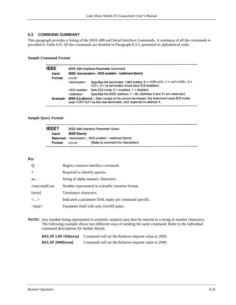
Lake Shore Model 475 Gaussmeter User’s Manual
Remote Operation 6-25
6.3 COMMAND SUMMARY This paragraph provides a listing of the IEEE-488 and Serial Interface Commands. A summary of all the commands is provided in Table 6-9. All the commands are detailed in Paragraph 6.3.1, presented in alphabetical order. Sample Command Format
Sample Query Format
Key
Q Begins common interface command.
? Required to identify queries.
aa… String of alpha numeric characters.
±nnn.nnnE±nn Number represented in scientific notation format.
[term] Terminator characters.
<…> Indicated a parameter field, many are command specific.
<state> Parameter field with only On/Off states. NOTE: Any number being represented in scientific notation may also be entered as a string of number characters.
The following example shows two different ways of sending the same command. Refer to the individual command descriptions for further details. RELSP 2.0E+03[term] Command will set the Relative setpoint value to 2000. RELSP 2000[term] Command will set the Relative setpoint value to 2000.
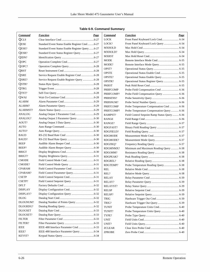
Lake Shore Model 475 Gaussmeter User’s Manual
6-26 Remote Operation
Table 6-9. Command Summary
Command Function Page QCLS Clear Interface Cmd ..............................................6-27 QESE Standard Event Status Enable Register Cmd .........6-27 QESE? Standard Event Status Enable Register Query .......6-27 QESR? Standard Event Status Register Query ...................6-27 QIDN? Identification Query ..............................................6-27 QOPC Operation Complete Cmd ......................................6-27 QOPC? Operation Complete Query ....................................6-28 QRST Reset Instrument Cmd ...........................................6-28 QSRE Service Request Enable Register Cmd ..................6-28 QSRE? Service Request Enable Register Query ................6-28 QSTB? Status Byte Query ..................................................6-28 QTRG Trigger Event ........................................................6-28 QTST? Self-Test Query .....................................................6-28 QWAI Wait-To-Continue Cmd .........................................6-28 ALARM Alarm Parameter Cmd ...........................................6-29 ALARM? Alarm Parameter Query .........................................6-29 ALARMST? Alarm Status Query ...............................................6-29 ANALOG Analog Output 3 Parameter Cmd...........................6-29 ANALOG? Analog Output 3 Parameter Query ........................6-30 AOUT? Analog Output 3 Data Query .................................6-30 AUTO Auto Range Command ..........................................6-30 AUTO? Auto Range Query .................................................6-30 BAUD RS-232 Baud Rate Cmd ........................................6-30 BAUD? RS-232 Baud Rate Query ......................................6-30 BEEP Audible Alarm Beeper Cmd ..................................6-30 BEEP? Audible Alarm Beeper Query ................................6-30 BRIGT Display Brightness Cmd ........................................6-30 BRIGT? Display Brightness Query ......................................6-31 CMODE Field Control Mode Cmd .......................................6-31 CMODE? Field Control Mode Query ....................................6-31 CPARAM Field Control Parameter Cmd ................................6-31 CPARAM? Field Control Parameter Query ..............................6-31 CSETP Field Control Setpoint Cmd ...................................6-31 CSETP? Field Control Setpoint Query ................................6-31 DFLT Factory Defaults Cmd ...........................................6-32 DISPLAY Display Configuration Cmd ...................................6-32 DISPLAY? Display Configuration Query ................................6-32 DLOG Datalog Start Cmd .................................................6-32 DLOGNUM? Datalog Number of Points Query ..........................6-32 DLOGRDG? Datalog Reading Query .........................................6-32 DLOGSET Datalog Rate Cmd .................................................6-33 DLOGSET? Datalog Rate Query ...............................................6-33 FILTER Filter Parameter Cmd ............................................6-33 FILTER? Filter Parameter Query ..........................................6-33 IEEE IEEE-488 Interface Parameter Cmd ......................6-33 IEEE? IEEE-488 Interface Parameter Query ....................6-34 KEYST? Keypad Status Query .............................................6-34
Command Function Page LOCK Front Panel Keyboard Lock Cmd........................ 6-34 LOCK? Front Panel Keyboard Lock Query ..................... 6-34 MXHOLD Max Hold Cmd ................................................... 6-34 MXHOLD? Max Hold Query ................................................. 6-34 MXRST Max Hold Reset Cmd.......................................... 6-34 MODE Remote Interface Mode Cmd .............................. 6-35 MODE? Remote Interface Mode Query ............................ 6-35 OPST? Operational Status Query .................................... 6-35 OPSTE Operational Status Enable Cmd .......................... 6-35 OPSTE? Operational Status Enable Query ........................ 6-35 OPSTR? Operational Status Register Query ...................... 6-35 PKRST Peak Hold Reset Cmd ......................................... 6-35 PRBFCOMP Probe Field Compensation Cmd ......................... 6-36 PRBFCOMP? Probe Field Compensation Query ....................... 6-36 PRBSENS? Probe Sensitivity Query ...................................... 6-36 PRBSNUM? Probe Serial Number Query ................................ 6-36 PRBTCOMP Probe Temperature Compensation Cmd ............. 6-36 PRBTCOMP? Probe Temperature Compensation Query ........... 6-36 RAMPST? Field Control Setpoint Ramp Status Query ......... 6-36 RANGE Field Range Cmd ................................................ 6-36 RANGE? Field Range Query .............................................. 6-37 RDGFAST? Binary Field Reading Query ............................... 6-37 RDGFIELD? Field Reading Query ........................................... 6-37 RDGMODE Measurement Mode Cmd .................................... 6-37 RDGMODE? Measurement Mode Query .................................. 6-37 RDGFRQ? Frequency Reading Query .................................. 6-37 RDGMNMX? Minimum and Maximum Reading Query ........... 6-38 RDGOHM? Resistance Reading Query .................................. 6-38 RDGPEAK? Peak Reading Query ........................................... 6-38 RDGREL? Relative Reading Query ...................................... 6-38 RDGTEMP? Probe Temperature Reading Query ..................... 6-38 REL Relative Mode Cmd ............................................ 6-38 REL? Relative Mode Query .......................................... 6-38 RELAY Relay Parameter Cmd ......................................... 6-39 RELAY? Relay Parameter Query ....................................... 6-39 RELAYST? Relay Status Query ............................................. 6-39 RELSP Relative Setpoint Cmd ........................................ 6-39 RELSP? Relative Setpoint Query ...................................... 6-39 TRIG Hardware Trigger Out Cmd ................................ 6-39 TRIG? Hardware Trigger Out Query .............................. 6-39 TUNIT Probe Temperature Units Cmd ............................ 6-40 TUNIT? Probe Temperature Units Query ......................... 6-40 TYPE? Probe Type Query ............................................... 6-40 UNIT Field Units Cmd .................................................. 6-40 UNIT? Field Units Query................................................ 6-40 ZCLEAR Clear Zero Probe Cmd ........................................ 6-40 ZPROBE Zero Probe Cmd .................................................. 6-40

Lake Shore Model 475 Gaussmeter User’s Manual
Remote Operation 6-27
6.3.1 Interface Commands (Alphabetical Listing)
*CLS Clear Interface Command Input: *CLS [term] Remarks: Clears the bits in the Standard Event Status Register and Operation Event Register and terminates all
pending operations. Clears the interface, but not the instrument. The related instrument command is *RST.
*ESE Standard Event Status Enable Register Command Input: *ESE <bit weighting>[term] Format: nnn Remarks: The Standard Event Status Enable Register determines which bits in the Standard Event Status
Register will set the summary bit in the Status Byte. This command programs the enable register using a decimal value which corresponds to the binary-weighted sum of all bits in the register. Refer to Paragraph 6.1.4.2.1.
*ESE? Standard Event Status Enable Register Query Input: *ESE? [term] Returned: <bit weighting>[term] Format: nnn (Refer to command for description)
*ESR? Standard Event Status Register Query Input: *ESR? [term] Returned: <bit weighting> Format: nnn Remarks: Bits in this register correspond to various system events and latch when the event occurs. When an
event bit is set, subsequent events corresponding to that bit are ignored. Set bits remain latched until the register is reset by this query or a *CLS command. Refer to Paragraph 6.1.4.2.1.
*IDN? Identification Query Input: *IDN? [term] Returned: <manufacturer>,<model>,<serial>,<date>[term] Format: aaaa,aaaaaaaa,aaaaaaa,mmddyyyy
<manufacture> Manufacturer ID <model> Instrument model number <serial> Serial number <date> Instrument firmware revision date
Example: LSCI,MODEL475,1234567,06122003
*OPC Operation Complete Command Input: *OPC [term] Remarks: Used in conjunction with bit 0 (OPC of the Standard Event Status Register. If sent as the last command
in a command sequence, bit 0 will be set when the instrument completes the operation that was initiated by the command sequence. Refer to Paragraph 6.1.4.3.6 for more information.
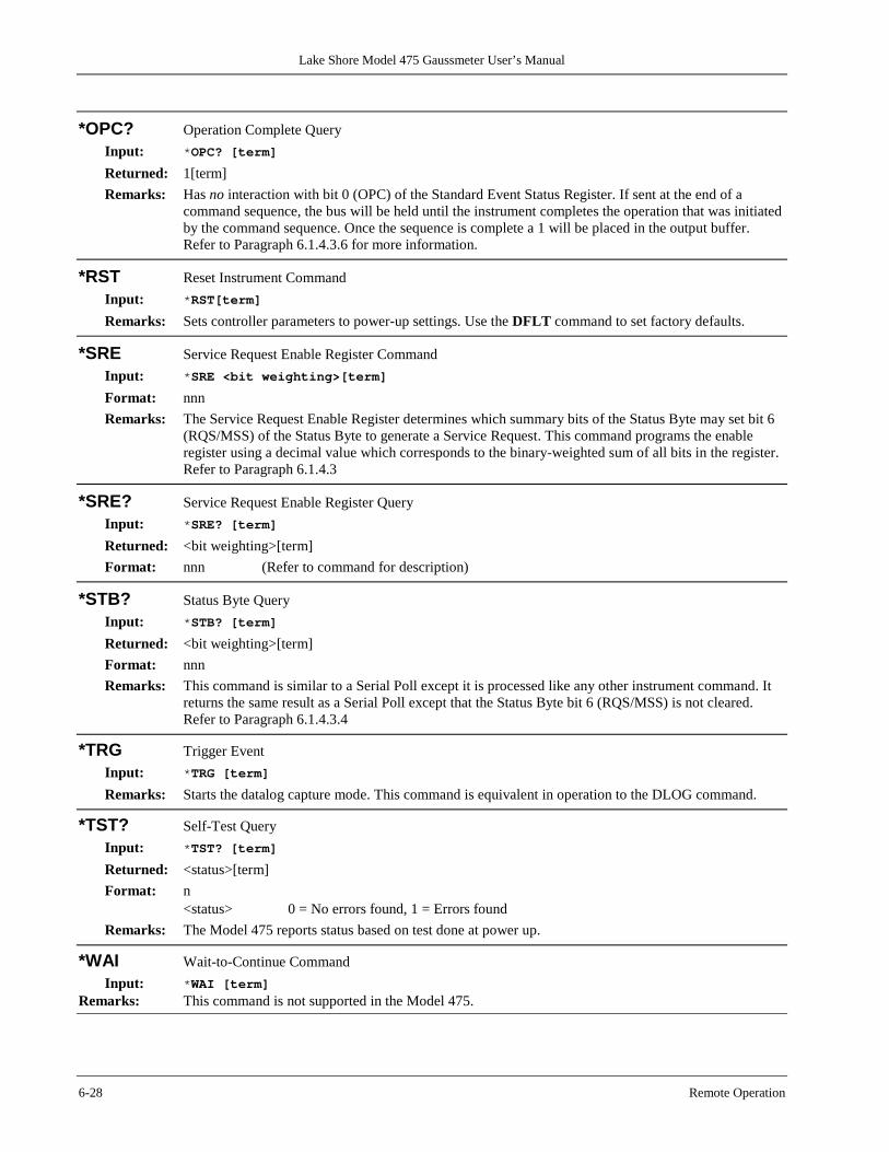
Lake Shore Model 475 Gaussmeter User’s Manual
6-28 Remote Operation
*OPC? Operation Complete Query Input: *OPC? [term] Returned: 1[term] Remarks: Has no interaction with bit 0 (OPC) of the Standard Event Status Register. If sent at the end of a
command sequence, the bus will be held until the instrument completes the operation that was initiated by the command sequence. Once the sequence is complete a 1 will be placed in the output buffer. Refer to Paragraph 6.1.4.3.6 for more information.
*RST Reset Instrument Command Input: *RST[term] Remarks: Sets controller parameters to power-up settings. Use the DFLT command to set factory defaults.
*SRE Service Request Enable Register Command Input: *SRE <bit weighting>[term] Format: nnn Remarks: The Service Request Enable Register determines which summary bits of the Status Byte may set bit 6
(RQS/MSS) of the Status Byte to generate a Service Request. This command programs the enable register using a decimal value which corresponds to the binary-weighted sum of all bits in the register. Refer to Paragraph 6.1.4.3
*SRE? Service Request Enable Register Query Input: *SRE? [term] Returned: <bit weighting>[term] Format: nnn (Refer to command for description)
*STB? Status Byte Query Input: *STB? [term] Returned: <bit weighting>[term] Format: nnn Remarks: This command is similar to a Serial Poll except it is processed like any other instrument command. It
returns the same result as a Serial Poll except that the Status Byte bit 6 (RQS/MSS) is not cleared. Refer to Paragraph 6.1.4.3.4
*TRG Trigger Event Input: *TRG [term] Remarks: Starts the datalog capture mode. This command is equivalent in operation to the DLOG command.
*TST? Self-Test Query Input: *TST? [term] Returned: <status>[term] Format: n
<status> 0 = No errors found, 1 = Errors found Remarks: The Model 475 reports status based on test done at power up.
*WAI Wait-to-Continue Command Input: *WAI [term]
Remarks: This command is not supported in the Model 475.
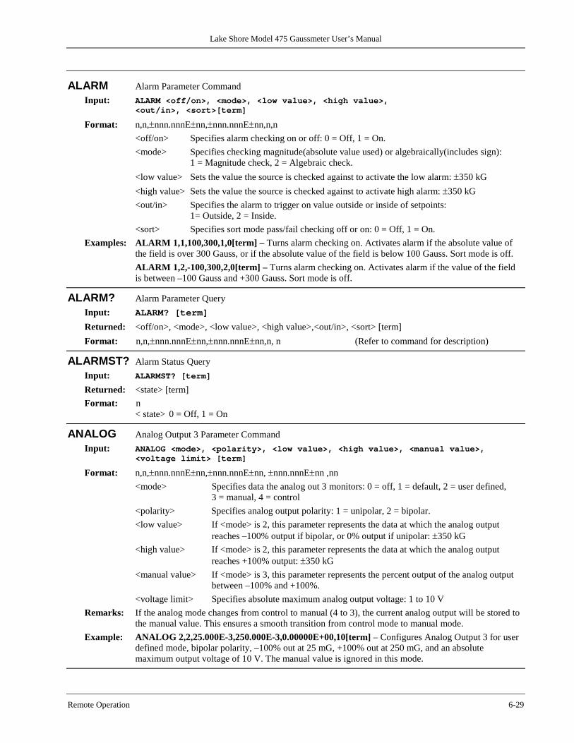
Lake Shore Model 475 Gaussmeter User’s Manual
Remote Operation 6-29
ALARM Alarm Parameter Command Input: ALARM <off/on>, <mode>, <low value>, <high value>,
<out/in>, <sort>[term] Format: n,n,±nnn.nnnE±nn,±nnn.nnnE±nn,n,n
<off/on> Specifies alarm checking on or off: 0 = Off, 1 = On. <mode> Specifies checking magnitude(absolute value used) or algebraically(includes sign):
1 = Magnitude check, 2 = Algebraic check. <low value> Sets the value the source is checked against to activate the low alarm: ±350 kG <high value> Sets the value the source is checked against to activate high alarm: ±350 kG <out/in> Specifies the alarm to trigger on value outside or inside of setpoints:
1= Outside, 2 = Inside. <sort> Specifies sort mode pass/fail checking off or on: 0 = Off, 1 = On.
Examples: ALARM 1,1,100,300,1,0[term] – Turns alarm checking on. Activates alarm if the absolute value of the field is over 300 Gauss, or if the absolute value of the field is below 100 Gauss. Sort mode is off. ALARM 1,2,-100,300,2,0[term] – Turns alarm checking on. Activates alarm if the value of the field is between –100 Gauss and +300 Gauss. Sort mode is off.
ALARM? Alarm Parameter Query Input: ALARM? [term] Returned: <off/on>, <mode>, <low value>, <high value>,<out/in>, <sort> [term] Format: n,n,±nnn.nnnE±nn,±nnn.nnnE±nn,n, n (Refer to command for description)
ALARMST? Alarm Status Query Input: ALARMST? [term] Returned: <state> [term] Format: n
< state> 0 = Off, 1 = On
ANALOG Analog Output 3 Parameter Command Input: ANALOG <mode>, <polarity>, <low value>, <high value>, <manual value>,
<voltage limit> [term] Format: n,n,±nnn.nnnE±nn,±nnn.nnnE±nn, ±nnn.nnnE±nn ,nn
<mode> Specifies data the analog out 3 monitors: 0 = off, 1 = default, 2 = user defined, 3 = manual, 4 = control
<polarity> Specifies analog output polarity: 1 = unipolar, 2 = bipolar. <low value> If <mode> is 2, this parameter represents the data at which the analog output
reaches –100% output if bipolar, or 0% output if unipolar: ±350 kG <high value> If <mode> is 2, this parameter represents the data at which the analog output
reaches +100% output: ±350 kG <manual value> If <mode> is 3, this parameter represents the percent output of the analog output
between –100% and +100%. <voltage limit> Specifies absolute maximum analog output voltage: 1 to 10 V
Remarks: If the analog mode changes from control to manual (4 to 3), the current analog output will be stored to the manual value. This ensures a smooth transition from control mode to manual mode.
Example: ANALOG 2,2,25.000E-3,250.000E-3,0.00000E+00,10[term] – Configures Analog Output 3 for user defined mode, bipolar polarity, –100% out at 25 mG, +100% out at 250 mG, and an absolute maximum output voltage of 10 V. The manual value is ignored in this mode.
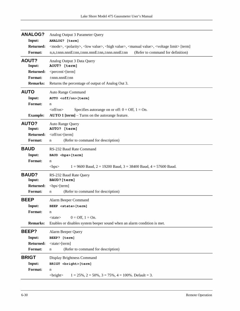
Lake Shore Model 475 Gaussmeter User’s Manual
6-30 Remote Operation
ANALOG? Analog Output 3 Parameter Query Input: ANALOG? [term] Returned: <mode>, <polarity>, <low value>, <high value>, <manual value>, <voltage limit> [term] Format: n,n,±nnn.nnnE±nn,±nnn.nnnE±nn,±nnn.nnnE±nn (Refer to command for definition)
AOUT? Analog Output 3 Data Query Input: AOUT? [term] Returned: <percent>[term] Format: ±nnn.nnnE±nn Remarks: Returns the percentage of output of Analog Out 3.
AUTO Auto Range Command Input: AUTO <off/on>[term] Format: n
<off/on> Specifies autorange on or off: 0 = Off, 1 = On. Example: AUTO 1 [term] – Turns on the autorange feature.
AUTO? Auto Range Query Input: AUTO? [term] Returned: <off/on>[term] Format: n (Refer to command for description)
BAUD RS-232 Baud Rate Command Input: BAUD <bps>[term] Format: n
<bps> 1 = 9600 Baud, 2 = 19200 Baud, 3 = 38400 Baud, 4 = 57600 Baud.
BAUD? RS-232 Baud Rate Query Input: BAUD?[term] Returned: <bps>[term] Format: n (Refer to command for description)
BEEP Alarm Beeper Command Input: BEEP <state>[term] Format: n
<state> 0 = Off, 1 = On. Remarks: Enables or disables system beeper sound when an alarm condition is met.
BEEP? Alarm Beeper Query Input: BEEP? [term] Returned: <state>[term] Format: n (Refer to command for description)
BRIGT Display Brightness Command Input: BRIGT <bright>[term] Format: n
<bright> 1 = 25%, 2 = 50%, 3 = 75%, 4 = 100%. Default = 3.
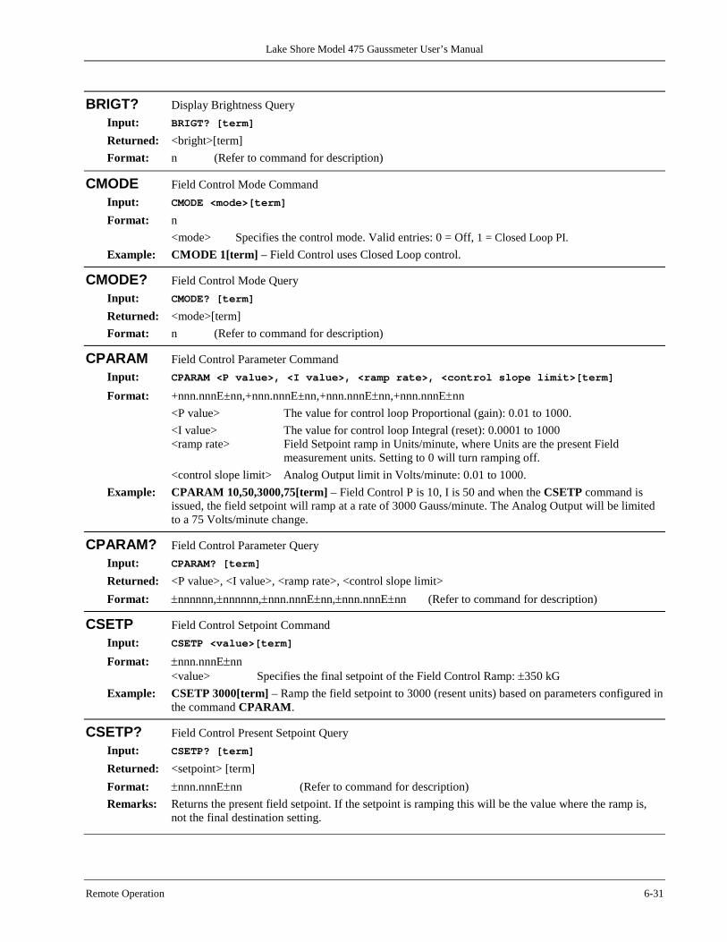
Lake Shore Model 475 Gaussmeter User’s Manual
Remote Operation 6-31
BRIGT? Display Brightness Query Input: BRIGT? [term] Returned: <bright>[term] Format: n (Refer to command for description)
CMODE Field Control Mode Command Input: CMODE <mode>[term] Format: n
<mode> Specifies the control mode. Valid entries: 0 = Off, 1 = Closed Loop PI. Example: CMODE 1[term] – Field Control uses Closed Loop control.
CMODE? Field Control Mode Query Input: CMODE? [term] Returned: <mode>[term] Format: n (Refer to command for description)
CPARAM Field Control Parameter Command Input: CPARAM <P value>, <I value>, <ramp rate>, <control slope limit>[term] Format: +nnn.nnnE±nn,+nnn.nnnE±nn,+nnn.nnnE±nn,+nnn.nnnE±nn
<P value> The value for control loop Proportional (gain): 0.01 to 1000. <I value> The value for control loop Integral (reset): 0.0001 to 1000 <ramp rate> Field Setpoint ramp in Units/minute, where Units are the present Field
measurement units. Setting to 0 will turn ramping off. <control slope limit> Analog Output limit in Volts/minute: 0.01 to 1000.
Example: CPARAM 10,50,3000,75[term] – Field Control P is 10, I is 50 and when the CSETP command is issued, the field setpoint will ramp at a rate of 3000 Gauss/minute. The Analog Output will be limited to a 75 Volts/minute change.
CPARAM? Field Control Parameter Query Input: CPARAM? [term] Returned: <P value>, <I value>, <ramp rate>, <control slope limit> Format: ±nnnnnn,±nnnnnn,±nnn.nnnE±nn,±nnn.nnnE±nn (Refer to command for description)
CSETP Field Control Setpoint Command Input: CSETP <value>[term] Format: ±nnn.nnnE±nn
<value> Specifies the final setpoint of the Field Control Ramp: ±350 kG Example: CSETP 3000[term] – Ramp the field setpoint to 3000 (resent units) based on parameters configured in
the command CPARAM.
CSETP? Field Control Present Setpoint Query Input: CSETP? [term] Returned: <setpoint> [term] Format: ±nnn.nnnE±nn (Refer to command for description) Remarks: Returns the present field setpoint. If the setpoint is ramping this will be the value where the ramp is,
not the final destination setting.

Lake Shore Model 475 Gaussmeter User’s Manual
6-32 Remote Operation
DFLT Factory Defaults Command Input: DFLT 99 [term]
Remarks: Sets all configuration values to factory defaults and resets the instrument. The "99" is included to prevent accidentally setting the unit to defaults.
DISPLAY Display Configuration Command Input: DISPLAY <item>[term] Format: n
<item> Specifies the item to display on line 2: 1 – 6 1 = Blank 2 = Field 3 = Probe Temperature and Frequency (if available) 4 = Relative setpoint 5 = Field Control setpoint 6 = Alarm Sort message
Example: DISPLAY 3[term] – Probe Temperature will be displayed on Line 2 if the probe is capable of measuring temperature. The Frequency will also be displayed if the Model 475 is in RMS mode.
DISPLAY? Display Configuration Query Input: DISPLAY? [term] Returned: <item>[term] Format: n (Refer to command for description)
DLOG Datalog Stop/Start Command Input: DLOG <stop/start> [term] Format: n
<stop/start> Starts and stops the datalog function: 0 = Stop, 1 = Start. Remarks: Use the DLOGSET command to set the datalog rate. The DLOGNUM? command can be used to
determine how many datalog points have been acquired.
DLOGNUM? Datalog Number of Points Query Input: DLOGNUM? [term] Returned: <num rdgs>[term] Format: nnnn
Remarks: Returns the number of field readings stored in the Datalog buffer.
DLOGRDG? Datalog Reading Query Input: DLOGRDG? <data point>[term] Format: nnnn <data point> Specifies data point to retrieve: 1 – 1024. Returned: <value>[term] Format: ±nnn.nnnE±nn
Remarks: Returns the field reading stored in the Datalog buffer at the point specified. Readings are in the field units the instrument is currently set to.

Lake Shore Model 475 Gaussmeter User’s Manual
Remote Operation 6-33
DLOGSET Datalog Rate Command Input: DLOGSET <rate> [term] Format: n
<rate> Configures the Datalog readings per second: 1 = 1 reading per second 2 = 10 readings per second 3 = 30 readings per second 4 = 100 readings per second 5 = 200 readings per second 6 = 400 readings per second 7 = 800 readings per second 8 = 1000 readings per second
DLOGSET? Datalog Rate Query Input: DLOGSET? [term] Returned: <rate> [term] Format: n (Refer to command for description)
FILTER Filter Parameter command Input: FILTER <rmsbpw>, <rmsbpn>, <rmslp>[term] Format: n,n,n
<rmsbpw> Selects center frequency of the RMS wide band filter: 1 = 100 Hz, 2 = 200 Hz, 3 = 400 Hz, 4 = 800 Hz, 5 = 1600 Hz, 6 = 3200 Hz, 7 = 6400 Hz, 8 = no filter.
<rmsbpn> Selects center frequency of the RMS narrow band filter: 1 = 50 Hz, 2 = 60 Hz, 3 = 100 Hz, 4 = 120 Hz, 5 = 200 Hz, 6 = 400 Hz, 7 = 800 Hz.
<rmslp> Selects corner frequency of the RMS low pass filter: 1 = 20 Hz, 2 = 60 Hz, 3 = 140 Hz.
Example: FILTER 3,5,2[term] – Configures the RMS wide band filter center frequency to 400 Hz, the RMS narrow band center frequency to 200 Hz, and the RMS low pass corner frequency to 60 Hz.
FILTER? Filter Parameter Query Input: FILTER? [term] Returned: <rmsbpw>, <rmsbpn>, <rmslp>[term] Format: n,n,n (Refer to command for description)
IEEE IEEE-488 Interface Parameter Command Input: IEEE <terminator>, <EOI enable>, <address>[term] Format: n,n,nn
<terminator> Specifies the terminator. Valid entries: 0 = <CR><LF>,1 = <LF><CR>, 2 = <LF>, 3 = no terminator (must have EOI enabled).
<EOI enable> Sets EOI mode: 0 = enabled, 1 = disabled. <address> Specifies the IEEE address: 1 – 30. (Address 0 and 31 are reserved.)
Example: IEEE 0,0,4[term] – After receipt of the current terminator, the instrument uses EOI mode, uses <CR><LF> as the new terminator, and responds to address 4.
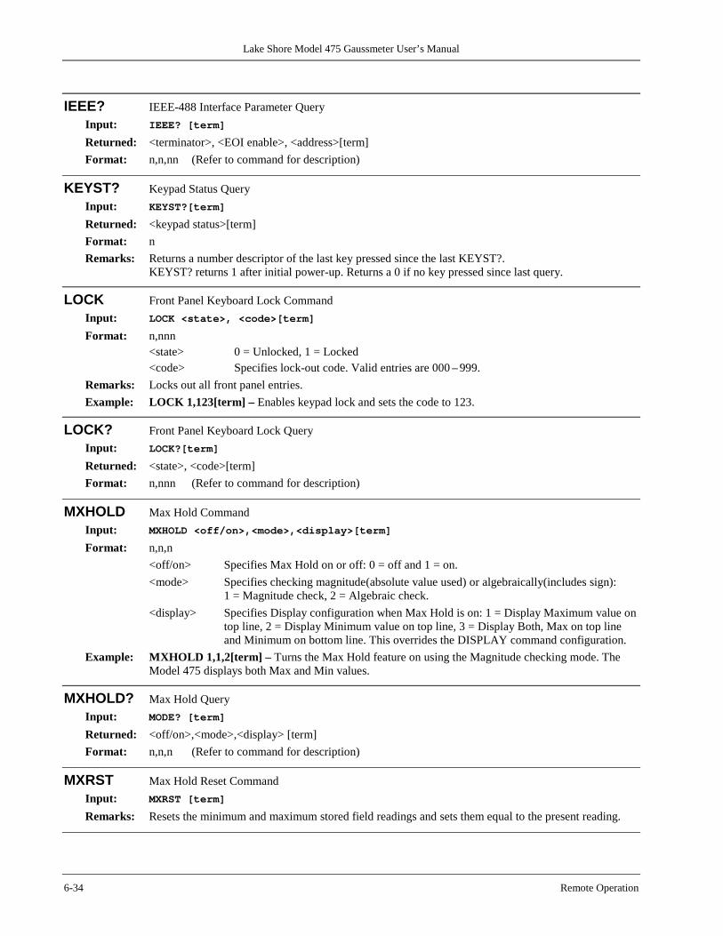
Lake Shore Model 475 Gaussmeter User’s Manual
6-34 Remote Operation
IEEE? IEEE-488 Interface Parameter Query Input: IEEE? [term] Returned: <terminator>, <EOI enable>, <address>[term] Format: n,n,nn (Refer to command for description)
KEYST? Keypad Status Query Input: KEYST?[term] Returned: <keypad status>[term] Format: n Remarks: Returns a number descriptor of the last key pressed since the last KEYST?.
KEYST? returns 1 after initial power-up. Returns a 0 if no key pressed since last query.
LOCK Front Panel Keyboard Lock Command Input: LOCK <state>, <code>[term] Format: n,nnn
<state> 0 = Unlocked, 1 = Locked <code> Specifies lock-out code. Valid entries are 000 – 999.
Remarks: Locks out all front panel entries. Example: LOCK 1,123[term] – Enables keypad lock and sets the code to 123.
LOCK? Front Panel Keyboard Lock Query Input: LOCK?[term] Returned: <state>, <code>[term] Format: n,nnn (Refer to command for description)
MXHOLD Max Hold Command Input: MXHOLD <off/on>,<mode>,<display>[term] Format: n,n,n
<off/on> Specifies Max Hold on or off: 0 = off and 1 = on. <mode> Specifies checking magnitude(absolute value used) or algebraically(includes sign):
1 = Magnitude check, 2 = Algebraic check. <display> Specifies Display configuration when Max Hold is on: 1 = Display Maximum value on
top line, 2 = Display Minimum value on top line, 3 = Display Both, Max on top line and Minimum on bottom line. This overrides the DISPLAY command configuration.
Example: MXHOLD 1,1,2[term] – Turns the Max Hold feature on using the Magnitude checking mode. The Model 475 displays both Max and Min values.
MXHOLD? Max Hold Query Input: MODE? [term] Returned: <off/on>,<mode>,<display> [term] Format: n,n,n (Refer to command for description)
MXRST Max Hold Reset Command Input: MXRST [term] Remarks: Resets the minimum and maximum stored field readings and sets them equal to the present reading.
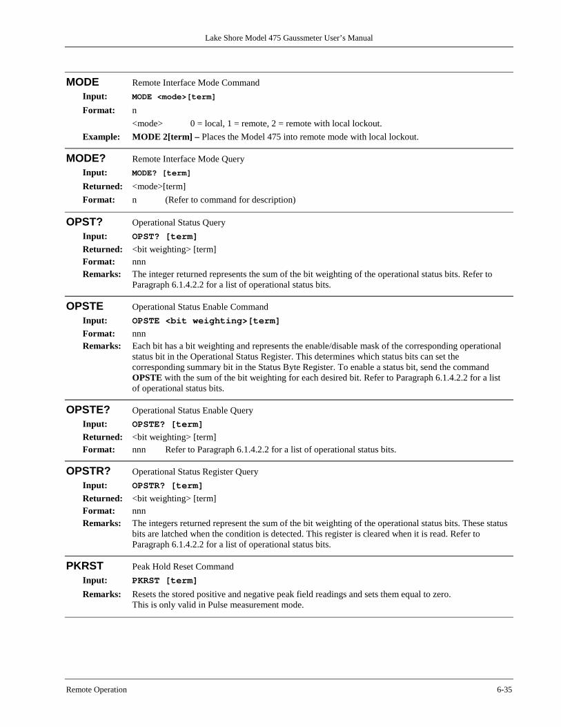
Lake Shore Model 475 Gaussmeter User’s Manual
Remote Operation 6-35
MODE Remote Interface Mode Command Input: MODE <mode>[term] Format: n
<mode> 0 = local, 1 = remote, 2 = remote with local lockout. Example: MODE 2[term] – Places the Model 475 into remote mode with local lockout.
MODE? Remote Interface Mode Query Input: MODE? [term] Returned: <mode>[term] Format: n (Refer to command for description)
OPST? Operational Status Query Input: OPST? [term] Returned: <bit weighting> [term]
Format: nnn Remarks: The integer returned represents the sum of the bit weighting of the operational status bits. Refer to
Paragraph 6.1.4.2.2 for a list of operational status bits.
OPSTE Operational Status Enable Command Input: OPSTE <bit weighting>[term] Format: nnn Remarks: Each bit has a bit weighting and represents the enable/disable mask of the corresponding operational
status bit in the Operational Status Register. This determines which status bits can set the corresponding summary bit in the Status Byte Register. To enable a status bit, send the command OPSTE with the sum of the bit weighting for each desired bit. Refer to Paragraph 6.1.4.2.2 for a list of operational status bits.
OPSTE? Operational Status Enable Query Input: OPSTE? [term] Returned: <bit weighting> [term] Format: nnn Refer to Paragraph 6.1.4.2.2 for a list of operational status bits.
OPSTR? Operational Status Register Query Input: OPSTR? [term] Returned: <bit weighting> [term]
Format: nnn Remarks: The integers returned represent the sum of the bit weighting of the operational status bits. These status
bits are latched when the condition is detected. This register is cleared when it is read. Refer to Paragraph 6.1.4.2.2 for a list of operational status bits.
PKRST Peak Hold Reset Command Input: PKRST [term] Remarks: Resets the stored positive and negative peak field readings and sets them equal to zero.
This is only valid in Pulse measurement mode.
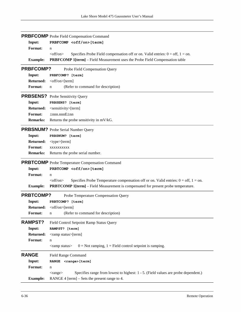
Lake Shore Model 475 Gaussmeter User’s Manual
6-36 Remote Operation
PRBFCOMP Probe Field Compensation Command Input: PRBFCOMP <off/on>[term] Format: n
<off/on> Specifies Probe Field compensation off or on. Valid entries: 0 = off, 1 = on. Example: PRBFCOMP 1[term] – Field Measurement uses the Probe Field Compensation table
PRBFCOMP? Probe Field Compensation Query Input: PRBFCOMP? [term] Returned: <off/on>[term] Format: n (Refer to command for description)
PRBSENS? Probe Sensitivity Query Input: PRBSENS? [term] Returned: <sensitivity>[term] Format: ±nnn.nnnE±nn Remarks: Returns the probe sensitivity in mV/kG.
PRBSNUM? Probe Serial Number Query Input: PRBSNUM? [term] Returned: <type>[term] Format: xxxxxxxxxx Remarks: Returns the probe serial number.
PRBTCOMP Probe Temperature Compensation Command Input: PRBTCOMP <off/on>[term] Format: n
<off/on> Specifies Probe Temperature compensation off or on. Valid entries: 0 = off, 1 = on. Example: PRBTCOMP 1[term] – Field Measurement is compensated for present probe temperature.
PRBTCOMP? Probe Temperature Compensation Query Input: PRBTCOMP? [term] Returned: <off/on>[term] Format: n (Refer to command for description)
RAMPST? Field Control Setpoint Ramp Status Query Input: RAMPST? [term] Returned: <ramp status>[term] Format: n
<ramp status> 0 = Not ramping, 1 = Field control setpoint is ramping.
RANGE Field Range Command Input: RANGE <range>[term] Format: n
<range> Specifies range from lowest to highest: 1 – 5. (Field values are probe dependent.) Example: RANGE 4 [term] – Sets the present range to 4.
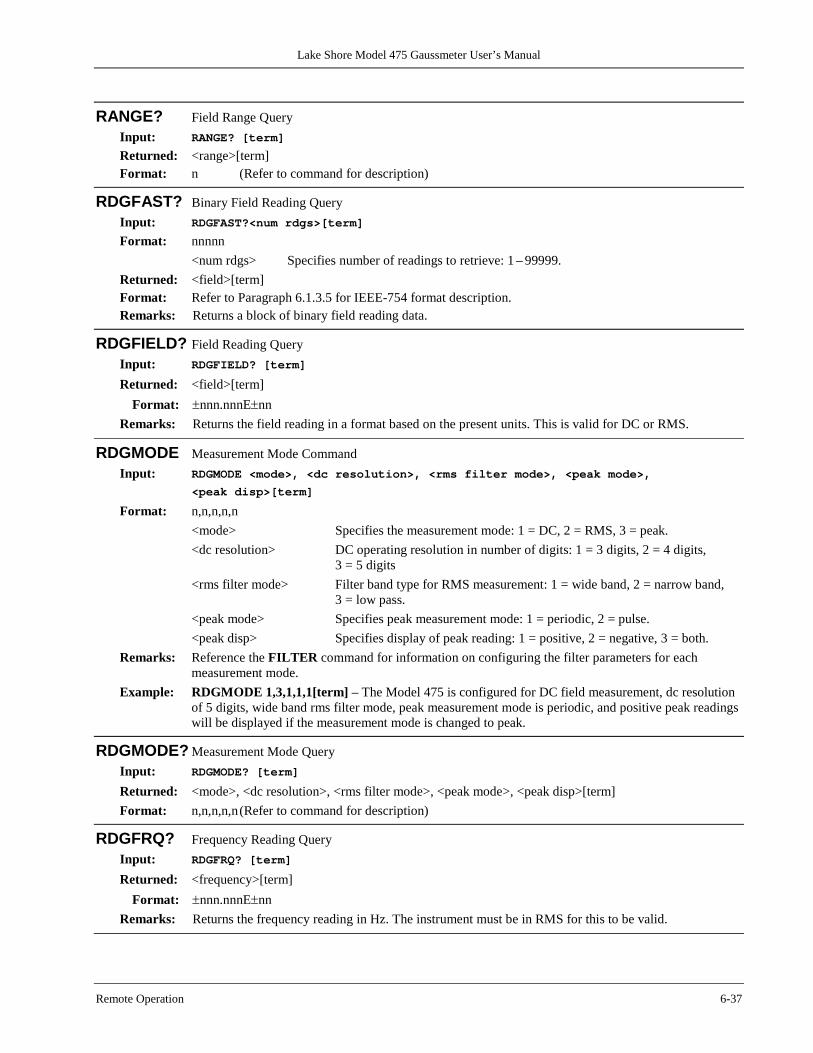
Lake Shore Model 475 Gaussmeter User’s Manual
Remote Operation 6-37
RANGE? Field Range Query Input: RANGE? [term] Returned: <range>[term] Format: n (Refer to command for description)
RDGFAST? Binary Field Reading Query Input: RDGFAST?<num rdgs>[term] Format: nnnnn <num rdgs> Specifies number of readings to retrieve: 1 – 99999. Returned: <field>[term] Format: Refer to Paragraph 6.1.3.5 for IEEE-754 format description. Remarks: Returns a block of binary field reading data.
RDGFIELD? Field Reading Query Input: RDGFIELD? [term] Returned: <field>[term]
Format: ±nnn.nnnE±nn Remarks: Returns the field reading in a format based on the present units. This is valid for DC or RMS.
RDGMODE Measurement Mode Command Input: RDGMODE <mode>, <dc resolution>, <rms filter mode>, <peak mode>,
<peak disp>[term] Format: n,n,n,n,n
<mode> Specifies the measurement mode: 1 = DC, 2 = RMS, 3 = peak. <dc resolution> DC operating resolution in number of digits: 1 = 3 digits, 2 = 4 digits,
3 = 5 digits <rms filter mode> Filter band type for RMS measurement: 1 = wide band, 2 = narrow band,
3 = low pass. <peak mode> Specifies peak measurement mode: 1 = periodic, 2 = pulse. <peak disp> Specifies display of peak reading: 1 = positive, 2 = negative, 3 = both.
Remarks: Reference the FILTER command for information on configuring the filter parameters for each measurement mode.
Example: RDGMODE 1,3,1,1,1[term] – The Model 475 is configured for DC field measurement, dc resolution of 5 digits, wide band rms filter mode, peak measurement mode is periodic, and positive peak readings will be displayed if the measurement mode is changed to peak.
RDGMODE? Measurement Mode Query Input: RDGMODE? [term] Returned: <mode>, <dc resolution>, <rms filter mode>, <peak mode>, <peak disp>[term] Format: n,n,n,n,n (Refer to command for description)
RDGFRQ? Frequency Reading Query Input: RDGFRQ? [term] Returned: <frequency>[term]
Format: ±nnn.nnnE±nn Remarks: Returns the frequency reading in Hz. The instrument must be in RMS for this to be valid.
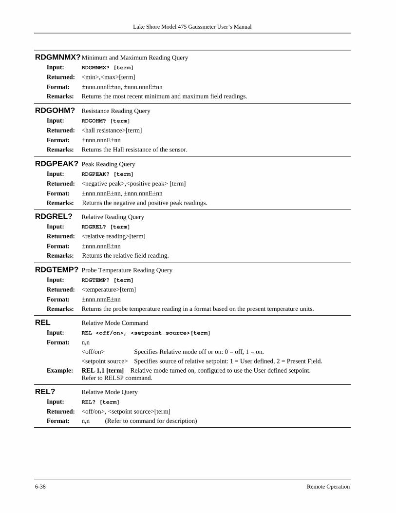
Lake Shore Model 475 Gaussmeter User’s Manual
6-38 Remote Operation
RDGMNMX? Minimum and Maximum Reading Query Input: RDGMNMX? [term] Returned: <min>,<max>[term] Format: ±nnn.nnnE±nn, ±nnn.nnnE±nn Remarks: Returns the most recent minimum and maximum field readings.
RDGOHM? Resistance Reading Query Input: RDGOHM? [term] Returned: <hall resistance>[term] Format: ±nnn.nnnE±nn Remarks: Returns the Hall resistance of the sensor.
RDGPEAK? Peak Reading Query Input: RDGPEAK? [term] Returned: <negative peak>,<positive peak> [term] Format: ±nnn.nnnE±nn, ±nnn.nnnE±nn Remarks: Returns the negative and positive peak readings.
RDGREL? Relative Reading Query Input: RDGREL? [term] Returned: <relative reading>[term] Format: ±nnn.nnnE±nn Remarks: Returns the relative field reading.
RDGTEMP? Probe Temperature Reading Query Input: RDGTEMP? [term]
Returned: <temperature>[term] Format: ±nnn.nnnE±nn Remarks: Returns the probe temperature reading in a format based on the present temperature units.
REL Relative Mode Command Input: REL <off/on>, <setpoint source>[term] Format: n,n
<off/on> Specifies Relative mode off or on: 0 = off, 1 = on. <setpoint source> Specifies source of relative setpoint: 1 = User defined, 2 = Present Field.
Example: REL 1,1 [term] – Relative mode turned on, configured to use the User defined setpoint. Refer to RELSP command.
REL? Relative Mode Query Input: REL? [term] Returned: <off/on>, <setpoint source>[term] Format: n,n (Refer to command for description)

Lake Shore Model 475 Gaussmeter User’s Manual
Remote Operation 6-39
RELAY Relay Parameter Command Input: RELAY <relay number>, <mode>, <alarm type>[term] Format: n,n,nn,n
<relay number> Specifies which relay to configure: 1 = Relay 1, 2 = Relay 2. <mode> Specifies relay mode: 0 = Off, 1 = On, 2 = Alarms. <alarm type> Specifies the alarm type that activates the relay when the relay is in alarm mode:
1 = Low Alarm, 2 = High Alarm, 3 = Both Alarms. Example: RELAY 1,2,2[term] – Relay 1 is setup in Alarms mode and activates when the low alarm activates.
RELAY? Relay Parameter Query Input: RELAY? <relay number>[term] Format: n
<relay number> Specifies which relay to query: 1–2. Returned: <mode>, <alarm type>[term] Format: n,n (Refer to command for description)
RELAYST? Relay Status Query Input: RELAYST? <relay number>[term] Format: n
<relay number> Specifies which relay to query: 1 = Relay 1, 2 = Relay 2. Returned: <status>[term] Format: n 0 = Off, 1 = On.
RELSP Relative Setpoint Command Input: RELSP <setpoint>[term] Format: ±nnn.nnnE±nn
<setpoint> Specifies the setpoint to use in the relative calculation: ±350 kG Example: RELSP 1200[term] – Configure the relative setpoint as 1200 Gauss(if units in Gauss). The relative
reading will use this value if relative is using the user defined setpoint. Refer to REL command.
RELSP? Relative Setpoint Query Input: RELSP? [term] Returned: <setpoint>[term] Format: ±nnn.nnnE±nn (Refer to command for description)
TRIG Hardware Trigger Out Command Input: TRIG <off/on>[term] Format: n
<off/on> Specifies hardware trigger off or on. Valid entries: 0 = Off, 1 = on. Example: TRIG 1[term] – The hardware trigger line produces a trigger when the instrument calculates a new
reading.
TRIG? Hardware Trigger Out Query Input: TRIG? [term] Returned: <off/on>[term] Format: n (Refer to command for description)
Lake Shore Model 475 Gaussmeter User’s Manual
6-40 Remote Operation
TUNIT Probe Temperature Units Command Input: TUNIT <units>[term] Format: n
<units> 1 = Celsius, 2 = Kelvin Example: TUNIT 1[term] – Configures the Model 475 to report probe temperature in °C.
TUNIT? Probe Temperature Units Query Input: TUNIT? [term] Returned: <units>[term] Format: n (Refer to command for description)
TYPE? Probe Type Query Input: TYPE? [term] Returned: <type>[term] Format: nn Remarks: Returns the probe type:
40 = high sensitivity 41 = high stability 42 = ultra-high sensitivity 50 = user programmable cable/high sensitivity probe 51 = user programmable cable/high stability probe 52 = user programmable cable/ultra-high sensitivity probe
UNIT Field Units Command Input: UNIT <units>[term] Format: n
<units> 1 = Gauss, 2 = Tesla, 3 = Oersted, 4 = Amp/meter. Example: UNIT 2[term] – Configures the Model 475 to report readings in Tesla.
UNIT? Field Units Query Input: UNIT? [term] Returned: <units>[term] Format: n (Refer to command for description)
ZCLEAR Clear Zero Probe Command Input: ZCLEAR [term] Remarks: Resets the value stored from the ZPROBE command.
ZPROBE Zero Probe Command Input: ZPROBE [term] Remarks: Initiates the Zero Probe function. Place the probe in zero gauss chamber before issuing this command.
Lake Shore Model 475 Gaussmeter User’s Manual
Probes and Accessories 7-1
CHAPTER 7
PROBES AND ACCESSORIES
7.0 GENERAL This chapter provides information on the accessories and probes available for the Model 475 DSP Gaussmeter.
7.1 MODELS The list of Model 475 Model numbers is provided as follows.
Model Description 475 Standard Model 475 DSP Gaussmeter. Power is configured as shown below.
Power Configurations. The instrument is configured at the factory for customer-selected power as follows.
1 100 V – US cord (NEMA 5-15) 2 120 V – US cord (NEMA 5-15 3 220 V –Euro cord (CEE 717) 4 240 V – Euro cord (CEE 717) 5 240 V – UK cord (BS 1363) 6 240 V – Swiss cord (SEV 1011) 7 220 V – China cord (G8 1002)
7.2 ACCESSORIES Accessories are devices that perform a secondary duty as an aid or refinement to the primary unit. A list of accessories available for the Model 475 is as follows:
Model Description of Accessories
G-106-253 * 25-pin D-Sub Plug. Used for I/O mating connector. G-106-264 * 25-pin D-Sub Shell. Used for I/O mating connector.
4005 IEEE-488 Cable Kit. One meter (3 feet) long IEEE-488 (GPIB) computer interface cable assembly. Includes extender required to use both IEEE cable and Auxiliary I/O connector simultaneously.
4060 * Standard Zero Gauss Chamber. For standard probe offset nulling. Size: 32 × 32 × 61 mm (1.3 × 1.3 × 2.4 in.). Bore: 12 mm diameter × 51 mm deep (0.5 × 2 in.). See Figure 7-17.
4065 Large Zero Gauss Chamber. For Gamma™ Probe offset nulling. Size: 57 × 53 × 305 mm (2.3 × 2 × 12 in.). Bore: 19 mm diameter × 279 mm deep (0.75 × 11 in.). See Figure 7-18.
MAN-475 * Model 475 Gaussmeter User’s Manual.
RM-1/2 Half-Rack Mounting Kit for One 1/2 Rack Gaussmeter. Half-length mounting panel and mounting ears to attach one Model 475 to a 483 mm (19-inch) rack mount space. See Figure 3-7.
RM-2 Dual Mounting Shelf for Two 1/2 Rack Gaussmeters. Mounting panel and mounting ears to attach two Model 475 DSP Gaussmeters to a 483 mm (19-inch) rack mount space. See Figure 3-8.
* Accessory included with a new Model 475.

Lake Shore Model 475 Gaussmeter User’s Manual
7-2 Probes and Accessories
7.3 LAKE SHORE STANDARD PROBES There are several types of Lake Shore Model 475 probes available: Axial, Gamma, Tangential, and Transverse — generally named for the Hall sensor orientation. Because the Model 475 covers such a wide magnetic field range (0.01 mG to 350 kG), three probe ranges are available: High Stability (HST), High Sensitivity (HSE), and Ultra-High Sensitivity (UHS). Please consult the factory for availability of probe types not detailed in this section.
7.3.1 Hall Probe Selection Criteria Proper selection of a Hall probe is probably the most difficult, and important, decision to make after choosing the Model 475. Utilizing the wrong probe may lead to less than optimal accuracy or, even worse, costly damage.
Probe Application Field measurement application is the controlling factor in probe selection. Application dictates the physical manifestation of the measured field, including the parameters described briefly below along with relevant probe characteristics. Magnitude: Typical Hall probes cover an operating range of four to five orders of field magnitude. Operation beyond this range often requires some compromise in performance, which is often higher noise or loss of resolution. Choosing the correct probe type ensures optimal performance in the desired measurement range.
High Sensitivity (HSE): High sensitivity probes are the most common for general-purpose field measurement. They operate effectively in fields up to 35 kG (3.5 T) with excellent sensitivity over their entire range. At low fields, their sensitivity can be as low as 5 mG (0.5 µT). HSE probes have a relatively small active area making them convenient for many applications and they are offered in a variety of stem geometries for convenience.
High Stability (HST): With a high field range of up to 350 kG (35 T), high stability probes are used when fields exceed the 35 kG (3.5 T) limit of HSE probes. Their low field performance is slightly degraded with minimum sensitivity of 50 mG (5 µT). High stability probes are also inherently more temperature stable than other probes and should be used when large temperature excursions are expected. The same probe geometries are available for both HST and HSE probes. HST probes are not to be used at frequencies above 800 Hz.
Ultra High Sensitivity (UHS): Low magnitude, large volume fields are most effectively measured with ultra high sensitivity probes that have unbeatable low field resolution to 20 µG (2 nT). UHS probes, or gamma probes, are ideal for measuring fringe fields or variations in Earth’s magnetic field. They should never be used in fields over 30 G. UHS probes are larger than other probes and they have a very large active area, making them impractical for small volume fields or tight spaces.
Orientation: Getting to the field is often much of the challenge in selecting a probe. Field orientation dictates the most basic probe geometry choice of transverse verses axial. Other variations are also available for less common, more challenging applications. Listed below are the standard configurations for HSE and HST probes, USH probes require special packaging that is not described here.
Transverse: Transverse probes, most often rectangular in shape, measure fields normal to their stem width. They are useful for most general-purpose field measurements and are essential for work in magnet gaps. Several stem lengths and thicknesses are available as standard probes.
Axial: Axial probes, most often round, measure fields normal to their end. They can also be used for general-purpose measurements but are most commonly used to measure fields produced by solenoids. Several stem lengths and diameters are available as standard probes.
Flexible: Flexible probes are special because they have a flexible portion in the middle of their stem. The active area at the tip remains rigid and somewhat exposed. (Flexible transverse probes are significantly more fragile than other transverse probes.) Flexible probes should only be select for applications that do not have direct access to the measured field with standard transverse or axial probes.
Lake Shore Model 475 Gaussmeter User’s Manual
Probes and Accessories 7-3
Tangential: Tangential probes are special transverse versions designed to measure fields parallel to and near a surface. The active area is very close to the stem tip. These probes are intended for this special application and should not be selected for general transverse measurements.
Multiple Axis: Multi-axis probes are available for multi-axis gaussmeters like the Lake Shore Model 460. These probes are not compatible with the Model 475.
Frequency: Hall-effect gaussmeters, like the Model 475, are equally well suited for measuring either static, DC fields or periodic, AC fields but proper probe selection is required to get optimal performance.
Metal Stem: Metal stem probes are the best choice for DC and low frequency AC measurements. Non-ferrous metals are used for probe stems because they provide the best protection for the delicate Hall-effect sensor. Aluminum is the most common metal stem material but brass can also be used. Metal stems do have one drawback; eddy currents are formed in them when they are placed in AC fields. These eddy currents oppose the field and cause measurement error. The error magnitude is proportional to frequency and is most noticeable above 800 Hz.
Non-metal Stem: Non-metal stems are required for higher frequency AC fields and for measuring pulse fields but they obviously provide less protection than metal stems. Fiberglass/epoxy is a common non-metal stem material or the Hall-effect sensor can be left exposed on its ceramic substrate. These materials are not conductive so eddy currents do not limit their frequency range but other factors may. Be careful to read and understand the frequency specification of both the probe and gaussmeter when choosing a non-metal probe.
WARNING: None of these probe types are suitable for direct exposure to high voltage. The possibility exists for damage to equipment or injury to the operator if the probe is exposed to high voltage.
Gradient: Probe selection would be easier if all fields were large and uniform but that is seldom the case because most fields are limited in volume and contain gradients (changes in magnitude). Hall-effect probes measure an average magnitude over their active area making it necessary to understand the relationship between active area and field gradients. Severe field gradients are always experienced as the active sense element is moved away from a permanent magnet pole making it important to know the distance between the active area and probe tip. The distance between probe tip and active area is specified for axial probes, but is less easily defined for transverse probes.
Nominal Active Area: HSE and HST probes have a nominal active area on the order of 1mm diameter, which is useful for all but the most stringent applications. The measured field is the average over the active area, but without severe gradients the measured value accurately represents the true field. Field mapping with standard probes is also practical if a mapping resolution of 1mm or greater is acceptable.
Small Active Area: HSE and HST probes with a smaller active area are also available from Lake Shore for measurements in severe gradients. They should also be chosen for high resolution mapping applications.
UHS Probes: UHS probes have a very large active length, up to 3.5 in. (8.9 cm). They are designed to measure large, ambient fields with little gradient.
Probe Durability All Hall effect probes are fragile. The sensor, normally located at the tip of the probe stem, must not be bent, physically shocked or abraded. Many users purchase probes with the thinnest transverse stem or smallest diameter axial stem thinking that these probes should fit all future applications. However, this may be a big mistake. Always use the most robust probe that fits the immediate application. For instance, the HMMT-6J04-VH (aluminum stem) is less prone to damage than the HMFT-3E03-VH (flexible stem). The HMMA-2502-VH (1/4-inch diameter aluminum) is more robust than the HMNA-1904-VH (3/16-inch diameter fiberglass) with its exposed Hall sensor. One last comment about probe handling, never fasten a probe stem to another object. If a probe is to be clamped, always clamp to the handle.
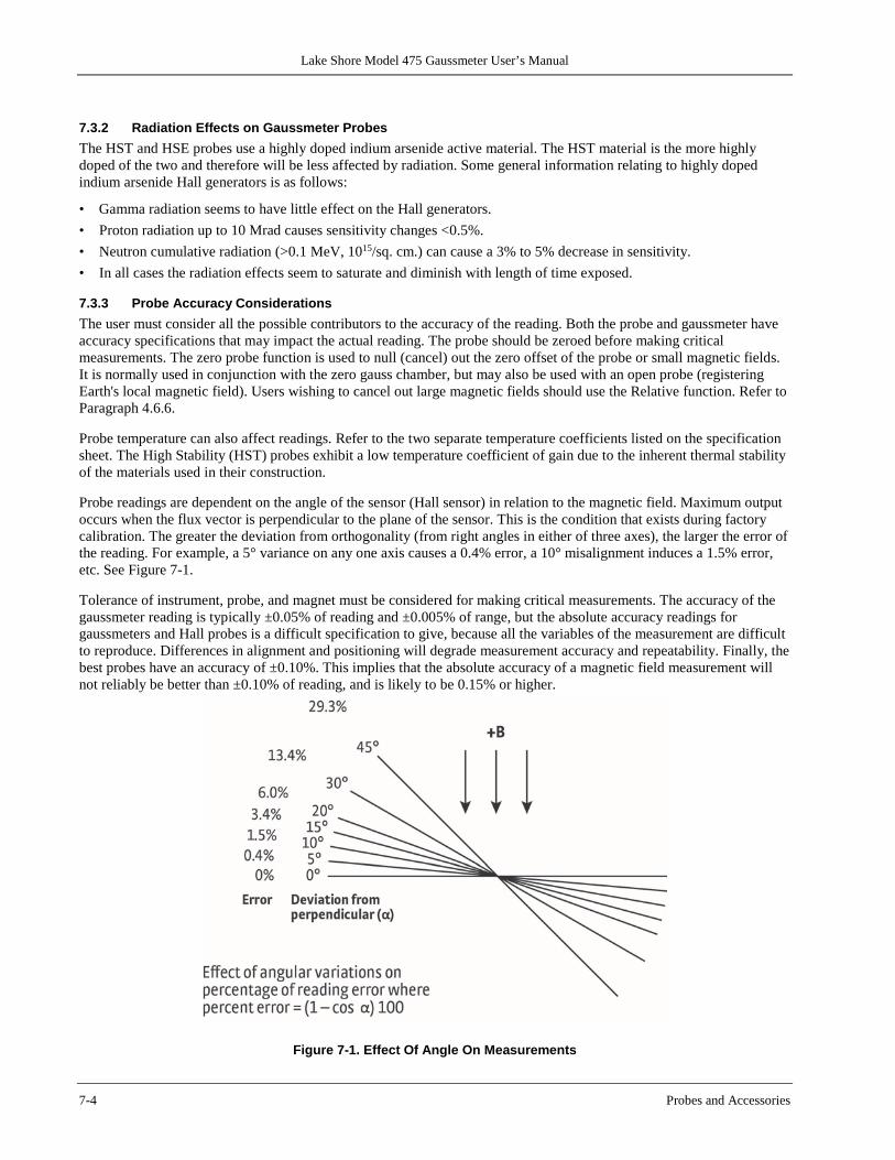
Lake Shore Model 475 Gaussmeter User’s Manual
7-4 Probes and Accessories
7.3.2 Radiation Effects on Gaussmeter Probes The HST and HSE probes use a highly doped indium arsenide active material. The HST material is the more highly doped of the two and therefore will be less affected by radiation. Some general information relating to highly doped indium arsenide Hall generators is as follows:
• Gamma radiation seems to have little effect on the Hall generators. • Proton radiation up to 10 Mrad causes sensitivity changes <0.5%. • Neutron cumulative radiation (>0.1 MeV, 1015/sq. cm.) can cause a 3% to 5% decrease in sensitivity. • In all cases the radiation effects seem to saturate and diminish with length of time exposed.
7.3.3 Probe Accuracy Considerations The user must consider all the possible contributors to the accuracy of the reading. Both the probe and gaussmeter have accuracy specifications that may impact the actual reading. The probe should be zeroed before making critical measurements. The zero probe function is used to null (cancel) out the zero offset of the probe or small magnetic fields. It is normally used in conjunction with the zero gauss chamber, but may also be used with an open probe (registering Earth's local magnetic field). Users wishing to cancel out large magnetic fields should use the Relative function. Refer to Paragraph 4.6.6. Probe temperature can also affect readings. Refer to the two separate temperature coefficients listed on the specification sheet. The High Stability (HST) probes exhibit a low temperature coefficient of gain due to the inherent thermal stability of the materials used in their construction. Probe readings are dependent on the angle of the sensor (Hall sensor) in relation to the magnetic field. Maximum output occurs when the flux vector is perpendicular to the plane of the sensor. This is the condition that exists during factory calibration. The greater the deviation from orthogonality (from right angles in either of three axes), the larger the error of the reading. For example, a 5° variance on any one axis causes a 0.4% error, a 10° misalignment induces a 1.5% error, etc. See Figure 7-1. Tolerance of instrument, probe, and magnet must be considered for making critical measurements. The accuracy of the gaussmeter reading is typically ±0.05% of reading and ±0.005% of range, but the absolute accuracy readings for gaussmeters and Hall probes is a difficult specification to give, because all the variables of the measurement are difficult to reproduce. Differences in alignment and positioning will degrade measurement accuracy and repeatability. Finally, the best probes have an accuracy of ±0.10%. This implies that the absolute accuracy of a magnetic field measurement will not reliably be better than ±0.10% of reading, and is likely to be 0.15% or higher.
Figure 7-1. Effect Of Angle On Measurements
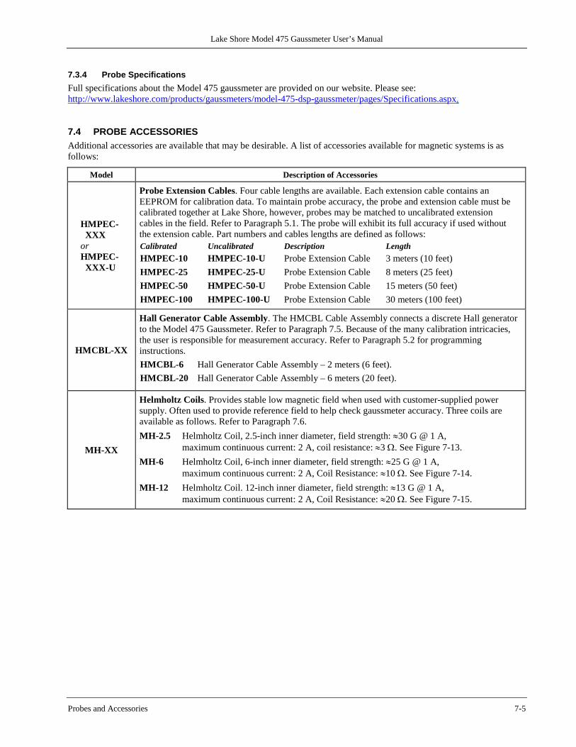
Lake Shore Model 475 Gaussmeter User’s Manual
Probes and Accessories 7-5
7.3.4 Probe Specifications Full specifications about the Model 475 gaussmeter are provided on our website. Please see: http://www.lakeshore.com/products/gaussmeters/model-475-dsp-gaussmeter/pages/Specifications.aspx.
7.4 PROBE ACCESSORIES Additional accessories are available that may be desirable. A list of accessories available for magnetic systems is as follows:
Model Description of Accessories
HMPEC- XXX or HMPEC- XXX-U
Probe Extension Cables. Four cable lengths are available. Each extension cable contains an EEPROM for calibration data. To maintain probe accuracy, the probe and extension cable must be calibrated together at Lake Shore, however, probes may be matched to uncalibrated extension cables in the field. Refer to Paragraph 5.1. The probe will exhibit its full accuracy if used without the extension cable. Part numbers and cables lengths are defined as follows: Calibrated Uncalibrated Description Length HMPEC-10 HMPEC-10-U Probe Extension Cable 3 meters (10 feet) HMPEC-25 HMPEC-25-U Probe Extension Cable 8 meters (25 feet) HMPEC-50 HMPEC-50-U Probe Extension Cable 15 meters (50 feet) HMPEC-100 HMPEC-100-U Probe Extension Cable 30 meters (100 feet)
HMCBL-XX
Hall Generator Cable Assembly. The HMCBL Cable Assembly connects a discrete Hall generator to the Model 475 Gaussmeter. Refer to Paragraph 7.5. Because of the many calibration intricacies, the user is responsible for measurement accuracy. Refer to Paragraph 5.2 for programming instructions. HMCBL-6 Hall Generator Cable Assembly – 2 meters (6 feet). HMCBL-20 Hall Generator Cable Assembly – 6 meters (20 feet).
MH-XX
Helmholtz Coils. Provides stable low magnetic field when used with customer-supplied power supply. Often used to provide reference field to help check gaussmeter accuracy. Three coils are available as follows. Refer to Paragraph 7.6. MH-2.5 Helmholtz Coil, 2.5-inch inner diameter, field strength: ≈30 G @ 1 A,
maximum continuous current: 2 A, coil resistance: ≈3 Ω. See Figure 7-13. MH-6 Helmholtz Coil, 6-inch inner diameter, field strength: ≈25 G @ 1 A,
maximum continuous current: 2 A, Coil Resistance: ≈10 Ω. See Figure 7-14. MH-12 Helmholtz Coil. 12-inch inner diameter, field strength: ≈13 G @ 1 A,
maximum continuous current: 2 A, Coil Resistance: ≈20 Ω. See Figure 7-15.
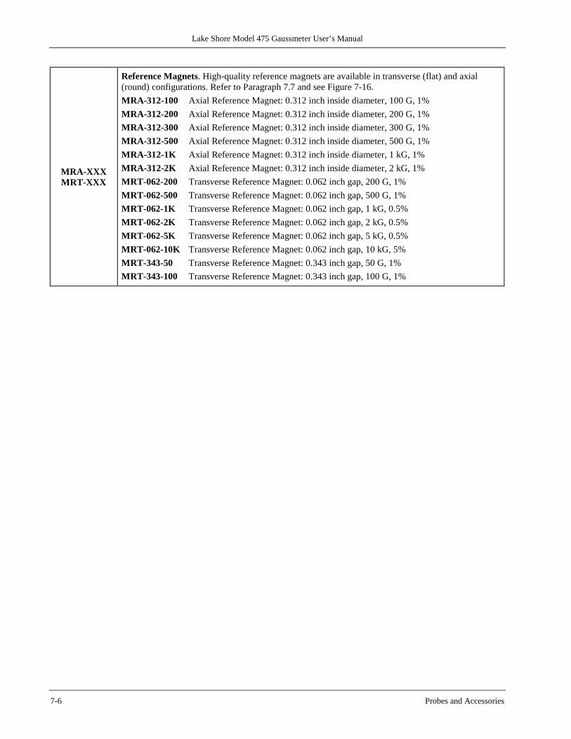
Lake Shore Model 475 Gaussmeter User’s Manual
7-6 Probes and Accessories
MRA-XXX MRT-XXX
Reference Magnets. High-quality reference magnets are available in transverse (flat) and axial (round) configurations. Refer to Paragraph 7.7 and see Figure 7-16. MRA-312-100 Axial Reference Magnet: 0.312 inch inside diameter, 100 G, 1% MRA-312-200 Axial Reference Magnet: 0.312 inch inside diameter, 200 G, 1% MRA-312-300 Axial Reference Magnet: 0.312 inch inside diameter, 300 G, 1% MRA-312-500 Axial Reference Magnet: 0.312 inch inside diameter, 500 G, 1% MRA-312-1K Axial Reference Magnet: 0.312 inch inside diameter, 1 kG, 1% MRA-312-2K Axial Reference Magnet: 0.312 inch inside diameter, 2 kG, 1% MRT-062-200 Transverse Reference Magnet: 0.062 inch gap, 200 G, 1% MRT-062-500 Transverse Reference Magnet: 0.062 inch gap, 500 G, 1% MRT-062-1K Transverse Reference Magnet: 0.062 inch gap, 1 kG, 0.5% MRT-062-2K Transverse Reference Magnet: 0.062 inch gap, 2 kG, 0.5% MRT-062-5K Transverse Reference Magnet: 0.062 inch gap, 5 kG, 0.5% MRT-062-10K Transverse Reference Magnet: 0.062 inch gap, 10 kG, 5% MRT-343-50 Transverse Reference Magnet: 0.343 inch gap, 50 G, 1% MRT-343-100 Transverse Reference Magnet: 0.343 inch gap, 100 G, 1%
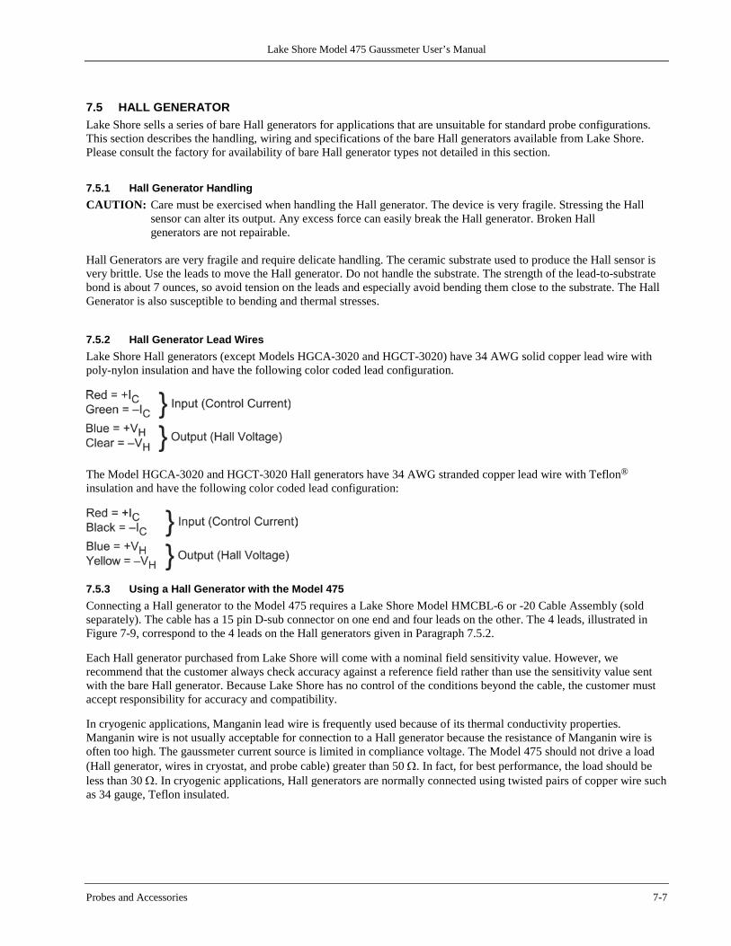
Lake Shore Model 475 Gaussmeter User’s Manual
Probes and Accessories 7-7
7.5 HALL GENERATOR Lake Shore sells a series of bare Hall generators for applications that are unsuitable for standard probe configurations. This section describes the handling, wiring and specifications of the bare Hall generators available from Lake Shore. Please consult the factory for availability of bare Hall generator types not detailed in this section.
7.5.1 Hall Generator Handling CAUTION: Care must be exercised when handling the Hall generator. The device is very fragile. Stressing the Hall
sensor can alter its output. Any excess force can easily break the Hall generator. Broken Hall generators are not repairable.
Hall Generators are very fragile and require delicate handling. The ceramic substrate used to produce the Hall sensor is very brittle. Use the leads to move the Hall generator. Do not handle the substrate. The strength of the lead-to-substrate bond is about 7 ounces, so avoid tension on the leads and especially avoid bending them close to the substrate. The Hall Generator is also susceptible to bending and thermal stresses.
7.5.2 Hall Generator Lead Wires Lake Shore Hall generators (except Models HGCA-3020 and HGCT-3020) have 34 AWG solid copper lead wire with poly-nylon insulation and have the following color coded lead configuration.
The Model HGCA-3020 and HGCT-3020 Hall generators have 34 AWG stranded copper lead wire with Teflon® insulation and have the following color coded lead configuration:
7.5.3 Using a Hall Generator with the Model 475 Connecting a Hall generator to the Model 475 requires a Lake Shore Model HMCBL-6 or -20 Cable Assembly (sold separately). The cable has a 15 pin D-sub connector on one end and four leads on the other. The 4 leads, illustrated in Figure 7-9, correspond to the 4 leads on the Hall generators given in Paragraph 7.5.2. Each Hall generator purchased from Lake Shore will come with a nominal field sensitivity value. However, we recommend that the customer always check accuracy against a reference field rather than use the sensitivity value sent with the bare Hall generator. Because Lake Shore has no control of the conditions beyond the cable, the customer must accept responsibility for accuracy and compatibility. In cryogenic applications, Manganin lead wire is frequently used because of its thermal conductivity properties. Manganin wire is not usually acceptable for connection to a Hall generator because the resistance of Manganin wire is often too high. The gaussmeter current source is limited in compliance voltage. The Model 475 should not drive a load (Hall generator, wires in cryostat, and probe cable) greater than 50 Ω. In fact, for best performance, the load should be less than 30 Ω. In cryogenic applications, Hall generators are normally connected using twisted pairs of copper wire such as 34 gauge, Teflon insulated.
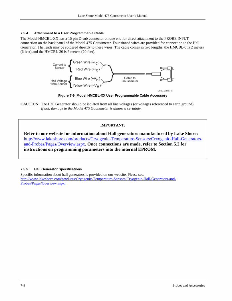
Lake Shore Model 475 Gaussmeter User’s Manual
7-8 Probes and Accessories
7.5.4 Attachment to a User Programmable Cable The Model HMCBL-XX has a 15 pin D-sub connector on one end for direct attachment to the PROBE INPUT connection on the back panel of the Model 475 Gaussmeter. Four tinned wires are provided for connection to the Hall Generator. The leads may be soldered directly to these wires. The cable comes in two lengths: the HMCBL-6 is 2 meters (6 feet) and the HMCBL-20 is 6 meters (20 feet).
MCBL_Cable.eps
Figure 7-9. Model HMCBL-XX User Programmable Cable Accessory CAUTION: The Hall Generator should be isolated from all line voltages (or voltages referenced to earth ground).
If not, damage to the Model 475 Gaussmeter is almost a certainty.
IMPORTANT:
Refer to our website for information about Hall generators manufactured by Lake Shore: http://www.lakeshore.com/products/Cryogenic-Temperature-Sensors/Cryogenic-Hall-Generators-and-Probes/Pages/Overview.aspx. Once connections are made, refer to Section 5.2 for instructions on programming parameters into the internal EPROM.
7.5.5 Hall Generator Specifications Specific information about hall generators is provided on our website. Please see: http://www.lakeshore.com/products/Cryogenic-Temperature-Sensors/Cryogenic-Hall-Generators-and-Probes/Pages/Overview.aspx.
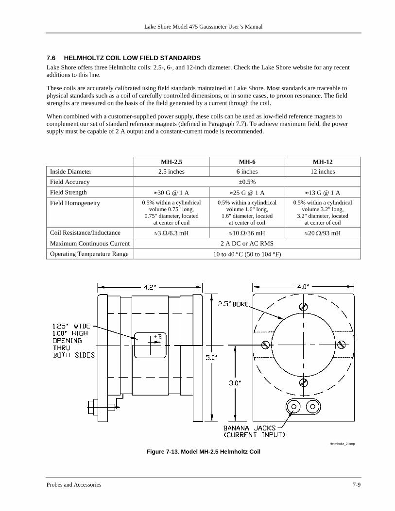
Lake Shore Model 475 Gaussmeter User’s Manual
Probes and Accessories 7-9
7.6 HELMHOLTZ COIL LOW FIELD STANDARDS Lake Shore offers three Helmholtz coils: 2.5-, 6-, and 12-inch diameter. Check the Lake Shore website for any recent additions to this line. These coils are accurately calibrated using field standards maintained at Lake Shore. Most standards are traceable to physical standards such as a coil of carefully controlled dimensions, or in some cases, to proton resonance. The field strengths are measured on the basis of the field generated by a current through the coil. When combined with a customer-supplied power supply, these coils can be used as low-field reference magnets to complement our set of standard reference magnets (defined in Paragraph 7.7). To achieve maximum field, the power supply must be capable of 2 A output and a constant-current mode is recommended.
MH-2.5 MH-6 MH-12 Inside Diameter 2.5 inches 6 inches 12 inches Field Accuracy ±0.5% Field Strength ≈30 G @ 1 A ≈25 G @ 1 A ≈13 G @ 1 A Field Homogeneity 0.5% within a cylindrical
volume 0.75" long, 0.75" diameter, located
at center of coil
0.5% within a cylindrical volume 1.6" long,
1.6" diameter, located at center of coil
0.5% within a cylindrical volume 3.2" long,
3.2" diameter, located at center of coil
Coil Resistance/Inductance ≈3 Ω/6.3 mH ≈10 Ω/36 mH ≈20 Ω/93 mH Maximum Continuous Current 2 A DC or AC RMS Operating Temperature Range 10 to 40 °C (50 to 104 °F)
Helmholtz_2.bmp
Figure 7-13. Model MH-2.5 Helmholtz Coil
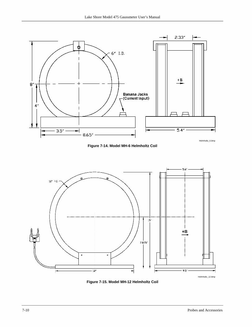
Lake Shore Model 475 Gaussmeter User’s Manual
7-10 Probes and Accessories
Helmholtz_6.bmp
Figure 7-14. Model MH-6 Helmholtz Coil
Helmholtz_12.bmp
Figure 7-15. Model MH-12 Helmholtz Coil
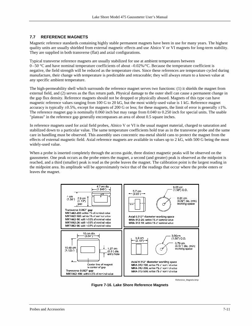
Lake Shore Model 475 Gaussmeter User’s Manual
Probes and Accessories 7-11
7.7 REFERENCE MAGNETS Magnetic reference standards containing highly stable permanent magnets have been in use for many years. The highest quality units are usually shielded from external magnetic effects and use Alnico V or VI magnets for long-term stability. They are supplied in both transverse (flat) and axial configurations. Typical transverse reference magnets are usually stabilized for use at ambient temperatures between 0 – 50 °C and have nominal temperature coefficients of about –0.02%/°C. Because the temperature coefficient is negative, the field strength will be reduced as the temperature rises. Since these references are temperature cycled during manufacture, their change with temperature is predictable and retraceable; they will always return to a known value at any specific ambient temperature. The high-permeability shell which surrounds the reference magnet serves two functions: (1) it shields the magnet from external field, and (2) serves as the flux return path. Physical damage to the outer shell can cause a permanent change in the gap flux density. Reference magnets should not be dropped or physically abused. Magnets of this type can have magnetic reference values ranging from 100 G to 20 kG, but the most widely-used value is 1 kG. Reference magnet accuracy is typically ±0.5%, except for magnets of 200 G or less; for these magnets, the limit of error is generally ±1%. The reference magnet gap is nominally 0.060 inch but may range from 0.040 to 0.250 inch for special units. The usable "plateau" in the reference gap generally encompasses an area of about 0.5 square inches. In reference magnets used for axial field probes, Alnico V or VI is the usual magnet material, charged to saturation and stabilized down to a particular value. The same temperature coefficients hold true as in the transverse probe and the same care in handling must be observed. This assembly uses concentric mu-metal shield cans to protect the magnet from the effects of external magnetic field. Axial reference magnets are available in values up to 2 kG, with 500 G being the most widely-used value. When a probe is inserted completely through the access guide, three distinct magnetic peaks will be observed on the gaussmeter. One peak occurs as the probe enters the magnet, a second (and greater) peak is observed as the midpoint is reached, and a third (smaller) peak is read as the probe leaves the magnet. The calibration point is the largest reading in the midpoint area. Its amplitude will be approximately twice that of the readings that occur where the probe enters or leaves the magnet.
Reference_Magnets.bmp
Figure 7-16. Lake Shore Reference Magnets
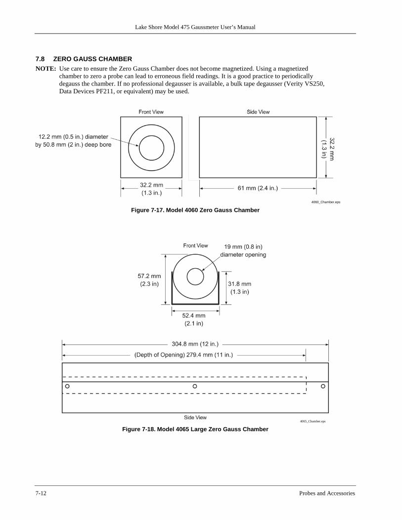
Lake Shore Model 475 Gaussmeter User’s Manual
7-12 Probes and Accessories
7.8 ZERO GAUSS CHAMBER NOTE: Use care to ensure the Zero Gauss Chamber does not become magnetized. Using a magnetized
chamber to zero a probe can lead to erroneous field readings. It is a good practice to periodically degauss the chamber. If no professional degausser is available, a bulk tape degausser (Verity VS250, Data Devices PF211, or equivalent) may be used.
4060_Chamber.eps
Figure 7-17. Model 4060 Zero Gauss Chamber
4065_Chamber.eps
Figure 7-18. Model 4065 Large Zero Gauss Chamber
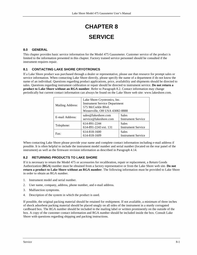
Lake Shore Model 475 Gaussmeter User’s Manual
Service 8-1
CHAPTER 8
SERVICE
8.0 GENERAL This chapter provides basic service information for the Model 475 Gaussmeter. Customer service of the product is limited to the information presented in this chapter. Factory trained service personnel should be consulted if the instrument requires repair.
8.1 CONTACTING LAKE SHORE CRYOTRONICS If a Lake Shore product was purchased through a dealer or representative, please use that resource for prompt sales or service information. When contacting Lake Shore directly, please specify the name of a department if do not know the name of an individual. Questions regarding product applications, price, availability and shipments should be directed to sales. Questions regarding instrument calibration or repair should be directed to instrument service. Do not return a product to Lake Shore without an RGA number. Refer to Paragraph 8.2. Contact information may change periodically but current contact information can always be found on the Lake Shore web site: www.lakeshore.com.
Mailing Address:
Lake Shore Cryotronics, Inc. Instrument Service Department 575 McCorkle Blvd. Westerville, OH USA 43082-8888
E-mail Address: [email protected] [email protected]
Sales Instrument Service
Telephone: 614-891-2244 614-891-2243 ext. 131
Sales Instrument Service
Fax: 614-818-1600 614-818-1609
Sales Instrument Service
When contacting Lake Shore please provide your name and complete contact information including e-mail address if possible. It is often helpful to include the instrument model number and serial number (located on the rear panel of the instrument) as well as the firmware revision information as described in Paragraph 4.14.
8.2 RETURNING PRODUCTS TO LAKE SHORE If it is necessary to return the Model 475 or accessories for recalibration, repair or replacement, a Return Goods Authorization (RGA) number must be obtained from a factory representative or from the Lake Shore web site. Do not return a product to Lake Shore without an RGA number. The following information must be provided to Lake Shore in order to obtain an RGA number. 1. Instrument model and serial number. 2. User name, company, address, phone number, and e-mail address. 3. Malfunction symptoms. 4. Description of the system in which the product is used. If possible, the original packing material should be retained for reshipment. If not available, a minimum of three inches of shock adsorbent packing material should be placed snugly on all sides of the instrument in a sturdy corrugated cardboard box. The RGA number should be included in the mailing label or written prominently on the outside of the box. A copy of the customer contact information and RGA number should be included inside the box. Consult Lake Shore with questions regarding shipping and packing instructions.
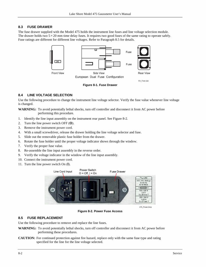
Lake Shore Model 475 Gaussmeter User’s Manual
8-2 Service
8.3 FUSE DRAWER The fuse drawer supplied with the Model 475 holds the instrument line fuses and line voltage selection module. The drawer holds two 5 × 20 mm time delay fuses. It requires two good fuses of the same rating to operate safely. Fuse ratings are different for different line voltages. Refer to Paragraph 8.5 for details.
EU_Fuse.eps
Figure 8-1. Fuse Drawer
8.4 LINE VOLTAGE SELECTION Use the following procedure to change the instrument line voltage selector. Verify the fuse value whenever line voltage is changed.
WARNING: To avoid potentially lethal shocks, turn off controller and disconnect it from AC power before performing this procedure.
1. Identify the line input assembly on the instrument rear panel. See Figure 8-2. 2. Turn the line power switch OFF (O). 3. Remove the instrument power cord. 4. With a small screwdriver, release the drawer holding the line voltage selector and fuse. 5. Slide out the removable plastic fuse holder from the drawer. 6. Rotate the fuse holder until the proper voltage indicator shows through the window. 7. Verify the proper fuse value. 8. Re-assemble the line input assembly in the reverse order. 9. Verify the voltage indicator in the window of the line input assembly. 10. Connect the instrument power cord. 11. Turn the line power switch On (l).
475_Power.bmp
Figure 8-2. Power Fuse Access
8.5 FUSE REPLACEMENT Use the following procedure to remove and replace the line fuses.
WARNING: To avoid potentially lethal shocks, turn off controller and disconnect it from AC power before performing these procedures.
CAUTION: For continued protection against fire hazard, replace only with the same fuse type and rating specified for the line for the line voltage selected.
Lake Shore Model 475 Gaussmeter User’s Manual
Service 8-3
Fuse Replacement (Continued)
NOTE: Test fuse with an ohmmeter. Do not rely on visual inspection of fuse.
1. Locate line input assembly on the instrument rear panel. See Figure 8-2. 2. Turn power switch Off (O). 3. Remove instrument power cord. 4. With a small screwdriver, release the drawer holding the line voltage selector and fuses. 5. Remove and discard both existing fuses. Replace with proper Slow-Blow (time-delay) fuse ratings as follows:
100/120V 0.5A 5 × 20 mm T 220/240V 0.25A 5 × 20 mm T
6. Re-assemble line input assembly in reverse order. 7. Verify voltage indicator in the line input assembly window. 8. Connect instrument power cord. 9. Turn power switch On (l).
8.6 ERROR MESSAGES The following messages appear on the instrument display when it identifies a problem during operation. The messages are divided into three groups. Instrument hardware messages are related to the instruments internal circuits or non-volatile memory. If one of these messages persists after power is cycled the instrument requires repair or recalibration. Measurement messages are most often associated with over field conditions caused by an improperly selected field range or excessive noise on the measurement leads, or a missing or illegal probe. If these messages persist after proper configuration, the instrument may require repair. Illegal operation messages remind the operator when a feature is locked out or the instrument is not configured to support a feature.
Instrument Hardware Defective RAM Internal RAM is defective and must be replaced
Invalid EEPROM EEPROM contents are corrupt and parameter values will be reset to default. Reoccurrence may indicate defective EEPROM. Calibration may be affected.
Input Not Responding Internal processor communication has failed.
Invalid Calibration
Instrument has not been calibrated or calibration memory has been corrupted. Recalibration is required for accurate measurements. Press the Escape and Enter keys simultaneously to clear the message. The instrument can still be used but it may not be operating within specifications.
Measurement No Probe There is no probe attached or the attached probe is damaged.
Invalid Probe The detected probe is not recognized as a valid Model 475 probe. Press Enter to continue.
Incompatible Probe A previous generation probe has been attached. Press Enter to continue. Measurement uses only nominal probe sensitivity. Accuracy not guaranteed.
OL The measured field is larger than the range. Increase the measurement range. Check probe zero.
SUNDER The temperature sensor reading is less than the minimum temperature table entry. SOVER The temperature sensor reading is greater than the maximum temperature table entry.
Illegal Operation *LOCKED* A key operation was attempted with the keypad locked. Not Available During Field Control
Certain operations are not allowed during Field Control.
Max Not Available With Peak
Max Hold and Peak do not operate together.
Invalid MPEC Cable Improper cable attached during the MPEC programming process. Invalid MCBL Cable Improper cable attached during the MCBL programming process.
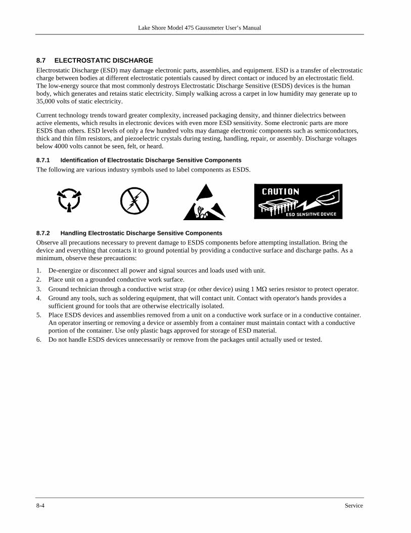
Lake Shore Model 475 Gaussmeter User’s Manual
8-4 Service
8.7 ELECTROSTATIC DISCHARGE Electrostatic Discharge (ESD) may damage electronic parts, assemblies, and equipment. ESD is a transfer of electrostatic charge between bodies at different electrostatic potentials caused by direct contact or induced by an electrostatic field. The low-energy source that most commonly destroys Electrostatic Discharge Sensitive (ESDS) devices is the human body, which generates and retains static electricity. Simply walking across a carpet in low humidity may generate up to 35,000 volts of static electricity. Current technology trends toward greater complexity, increased packaging density, and thinner dielectrics between active elements, which results in electronic devices with even more ESD sensitivity. Some electronic parts are more ESDS than others. ESD levels of only a few hundred volts may damage electronic components such as semiconductors, thick and thin film resistors, and piezoelectric crystals during testing, handling, repair, or assembly. Discharge voltages below 4000 volts cannot be seen, felt, or heard.
8.7.1 Identification of Electrostatic Discharge Sensitive Components The following are various industry symbols used to label components as ESDS.
8.7.2 Handling Electrostatic Discharge Sensitive Components Observe all precautions necessary to prevent damage to ESDS components before attempting installation. Bring the device and everything that contacts it to ground potential by providing a conductive surface and discharge paths. As a minimum, observe these precautions:
1. De-energize or disconnect all power and signal sources and loads used with unit. 2. Place unit on a grounded conductive work surface. 3. Ground technician through a conductive wrist strap (or other device) using 1 MΩ series resistor to protect operator. 4. Ground any tools, such as soldering equipment, that will contact unit. Contact with operator's hands provides a
sufficient ground for tools that are otherwise electrically isolated. 5. Place ESDS devices and assemblies removed from a unit on a conductive work surface or in a conductive container.
An operator inserting or removing a device or assembly from a container must maintain contact with a conductive portion of the container. Use only plastic bags approved for storage of ESD material.
6. Do not handle ESDS devices unnecessarily or remove from the packages until actually used or tested.
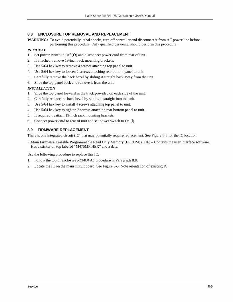
Lake Shore Model 475 Gaussmeter User’s Manual
Service 8-5
8.8 ENCLOSURE TOP REMOVAL AND REPLACEMENT WARNING: To avoid potentially lethal shocks, turn off controller and disconnect it from AC power line before
performing this procedure. Only qualified personnel should perform this procedure. REMOVAL 1. Set power switch to Off (O) and disconnect power cord from rear of unit. 2. If attached, remove 19-inch rack mounting brackets. 3. Use 5/64 hex key to remove 4 screws attaching top panel to unit. 4. Use 5/64 hex key to loosen 2 screws attaching rear bottom panel to unit. 5. Carefully remove the back bezel by sliding it straight back away from the unit. 6. Slide the top panel back and remove it from the unit. INSTALLATION 1. Slide the top panel forward in the track provided on each side of the unit. 2. Carefully replace the back bezel by sliding it straight into the unit. 3. Use 5/64 hex key to install 4 screws attaching top panel to unit. 4. Use 5/64 hex key to tighten 2 screws attaching rear bottom panel to unit. 5. If required, reattach 19-inch rack mounting brackets. 6. Connect power cord to rear of unit and set power switch to On (l).
8.9 FIRMWARE REPLACEMENT There is one integrated circuit (IC) that may potentially require replacement. See Figure 8-3 for the IC location.
• Main Firmware Erasable Programmable Read Only Memory (EPROM) (U16) – Contains the user interface software. Has a sticker on top labeled “M475MF.HEX” and a date.
Use the following procedure to replace this IC. 1. Follow the top of enclosure REMOVAL procedure in Paragraph 8.8. 2. Locate the IC on the main circuit board. See Figure 8-3. Note orientation of existing IC.
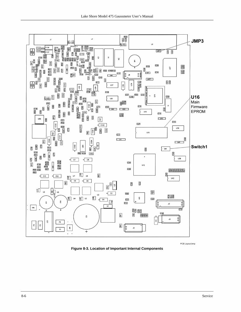
Lake Shore Model 475 Gaussmeter User’s Manual
8-6 Service
PCB Layout.bmp
Figure 8-3. Location of Important Internal Components
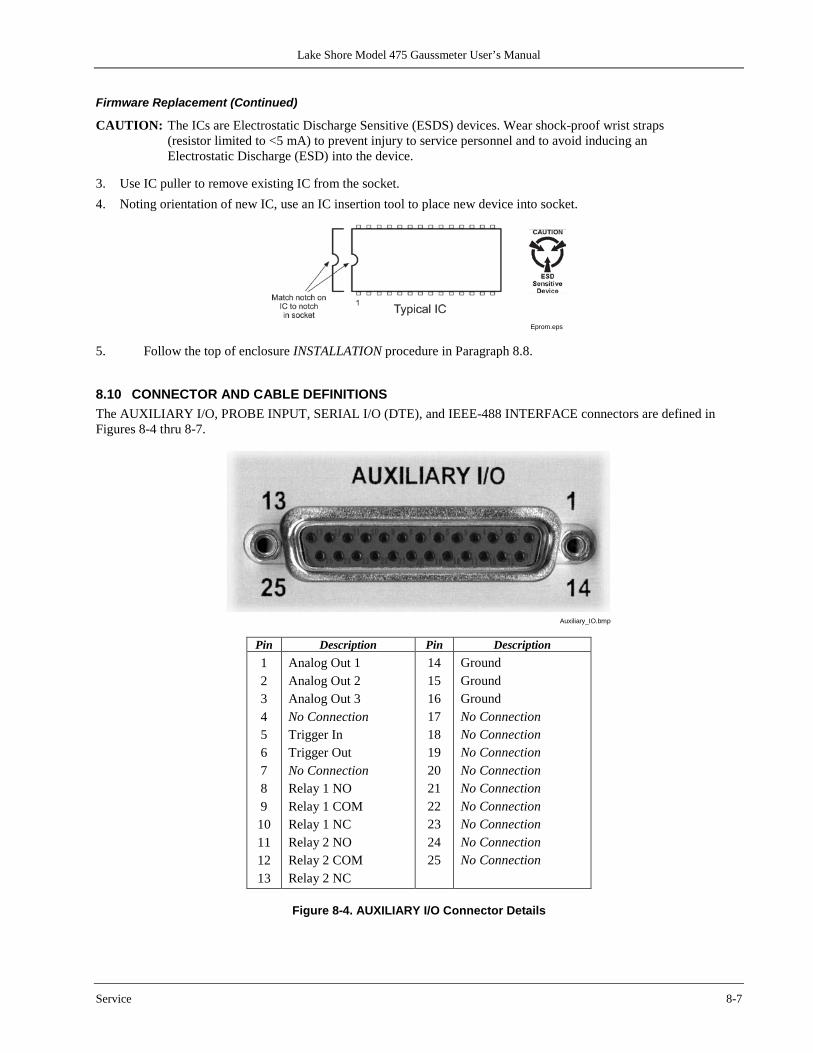
Lake Shore Model 475 Gaussmeter User’s Manual
Service 8-7
Firmware Replacement (Continued)
CAUTION: The ICs are Electrostatic Discharge Sensitive (ESDS) devices. Wear shock-proof wrist straps (resistor limited to <5 mA) to prevent injury to service personnel and to avoid inducing an Electrostatic Discharge (ESD) into the device.
3. Use IC puller to remove existing IC from the socket. 4. Noting orientation of new IC, use an IC insertion tool to place new device into socket.
Eprom.eps
5. Follow the top of enclosure INSTALLATION procedure in Paragraph 8.8.
8.10 CONNECTOR AND CABLE DEFINITIONS The AUXILIARY I/O, PROBE INPUT, SERIAL I/O (DTE), and IEEE-488 INTERFACE connectors are defined in Figures 8-4 thru 8-7.
Auxiliary_IO.bmp
Pin Description Pin Description 1 2 3 4 5 6 7 8 9 10 11 12 13
Analog Out 1 Analog Out 2 Analog Out 3 No Connection Trigger In Trigger Out No Connection Relay 1 NO Relay 1 COM Relay 1 NC Relay 2 NO Relay 2 COM Relay 2 NC
14 15 16 17 18 19 20 21 22 23 24 25
Ground Ground Ground No Connection No Connection No Connection No Connection No Connection No Connection No Connection No Connection No Connection
Figure 8-4. AUXILIARY I/O Connector Details

Lake Shore Model 475 Gaussmeter User’s Manual
8-8 Service
Probe_Input.bmp
Pin Description Pin Description 1 2 3 4 5 6 7 8
V input + No Connection V temp + I temp + I temp – V temp – No Connection I hall +
9 10 11 12 13 14 15
V input – No Connection EEPROM GND EEPROM VCC EEPROM CLK EEPROM DATA I hall –
Figure 8-5. PROBE INPUT Connector Details
Serial_IO.bmp
Model 475 Gaussmeter Typical Computers
SERIAL I/O (DTE) DB-25P (DTE) DE-9P (DTE) Pin Description Pin Description Pin Description 1 No Connection 2 TD (out) 1 DCD (in) 2 Receive Data (RD in) 3 RD (in) 2 RD (in) 3 Transmit Data (TD out) 4 RTS (out) 3 TD (out) 4 Data Terminal Ready (DTR out) 5 CTS (in) 4 DTR (out) 5 Ground (GND) 6 DSR (in) 5 GND 6 Data Set Ready (DSR in) 7 GND 6 DSR (in) 7 Data Terminal Ready (DTR out) (tied to 4) 8 DCD (in) 7 RTS (out) 8 No Connection 20 DTR (out) 8 CTS (in) 9 No Connection 22 Ring in (in) 9 Ring in (in)
Figure 8-6. SERIAL I/O (DTE) Connector Details
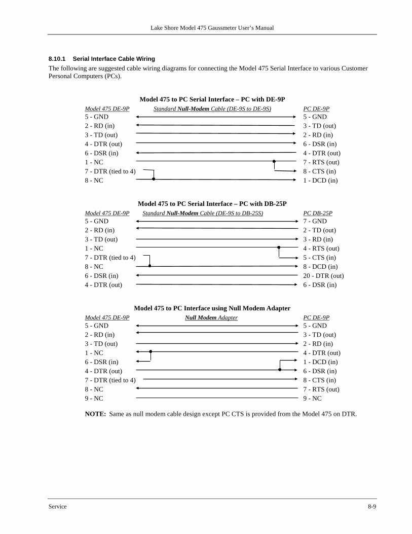
Lake Shore Model 475 Gaussmeter User’s Manual
Service 8-9
8.10.1 Serial Interface Cable Wiring The following are suggested cable wiring diagrams for connecting the Model 475 Serial Interface to various Customer Personal Computers (PCs).
Model 475 to PC Serial Interface – PC with DE-9P Model 475 DE-9P Standard Null-Modem Cable (DE-9S to DE-9S) PC DE-9P 5 - GND 5 - GND 2 - RD (in) 3 - TD (out) 3 - TD (out) 2 - RD (in) 4 - DTR (out) 6 - DSR (in) 6 - DSR (in) 4 - DTR (out) 1 - NC 7 - RTS (out) 7 - DTR (tied to 4) 8 - CTS (in) 8 - NC 1 - DCD (in)
Model 475 to PC Serial Interface – PC with DB-25P Model 475 DE-9P Standard Null-Modem Cable (DE-9S to DB-25S) PC DB-25P 5 - GND 7 - GND 2 - RD (in) 2 - TD (out) 3 - TD (out) 3 - RD (in) 1 - NC 4 - RTS (out) 7 - DTR (tied to 4) 5 - CTS (in) 8 - NC 8 - DCD (in) 6 - DSR (in) 20 - DTR (out) 4 - DTR (out) 6 - DSR (in)
Model 475 to PC Interface using Null Modem Adapter Model 475 DE-9P Null Modem Adapter PC DE-9P 5 - GND 5 - GND 2 - RD (in) 3 - TD (out) 3 - TD (out) 2 - RD (in) 1 - NC 4 - DTR (out) 6 - DSR (in) 1 - DCD (in) 4 - DTR (out) 6 - DSR (in) 7 - DTR (tied to 4) 8 - CTS (in) 8 - NC 7 - RTS (out) 9 - NC 9 - NC NOTE: Same as null modem cable design except PC CTS is provided from the Model 475 on DTR.
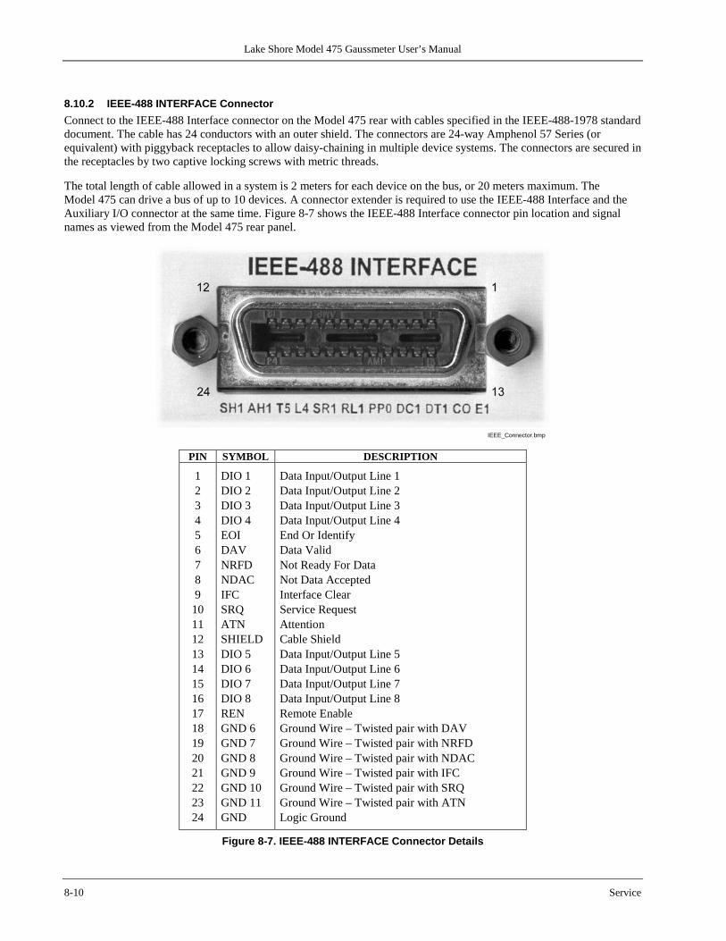
Lake Shore Model 475 Gaussmeter User’s Manual
8-10 Service
8.10.2 IEEE-488 INTERFACE Connector Connect to the IEEE-488 Interface connector on the Model 475 rear with cables specified in the IEEE-488-1978 standard document. The cable has 24 conductors with an outer shield. The connectors are 24-way Amphenol 57 Series (or equivalent) with piggyback receptacles to allow daisy-chaining in multiple device systems. The connectors are secured in the receptacles by two captive locking screws with metric threads. The total length of cable allowed in a system is 2 meters for each device on the bus, or 20 meters maximum. The Model 475 can drive a bus of up to 10 devices. A connector extender is required to use the IEEE-488 Interface and the Auxiliary I/O connector at the same time. Figure 8-7 shows the IEEE-488 Interface connector pin location and signal names as viewed from the Model 475 rear panel.
IEEE_Connector.bmp
PIN SYMBOL DESCRIPTION
1 2 3 4 5 6 7 8 9
10 11 12 13 14 15 16 17 18 19 20 21 22 23 24
DIO 1 DIO 2 DIO 3 DIO 4 EOI DAV NRFD NDAC IFC SRQ ATN SHIELD DIO 5 DIO 6 DIO 7 DIO 8 REN GND 6 GND 7 GND 8 GND 9 GND 10 GND 11 GND
Data Input/Output Line 1 Data Input/Output Line 2 Data Input/Output Line 3 Data Input/Output Line 4 End Or Identify Data Valid Not Ready For Data Not Data Accepted Interface Clear Service Request Attention Cable Shield Data Input/Output Line 5 Data Input/Output Line 6 Data Input/Output Line 7 Data Input/Output Line 8 Remote Enable Ground Wire – Twisted pair with DAV Ground Wire – Twisted pair with NRFD Ground Wire – Twisted pair with NDAC Ground Wire – Twisted pair with IFC Ground Wire – Twisted pair with SRQ Ground Wire – Twisted pair with ATN Logic Ground
Figure 8-7. IEEE-488 INTERFACE Connector Details
Lake Shore Model 475 Gaussmeter User’s Manual
Service 8-11
8.11 CALIBRATION PROCEDURE
8.11.1 Equipment Required for Calibration PC and Interface • PC with software loaded which provides serial command line communication.
(Example program in Paragraph 6.2.7 is ideal for this purpose.) • DE-9 to DE-9 cable. Pin to pin connections on all 9 pins. Female connectors on both ends. • DE-9 null modem adapter. Test and Measurement Equipment • Digital Voltmeter (DVM). Voltage and current specs to be equivalent to or better than HP3458 specs. • Function Generator. Frequency and voltage specs to be equivalent to or better than HP/Agilent 33120 specs. • One 332 Ω, 0.1%, 25 ppm resistor. • One 33.2 Ω, 0.1%, 25 ppm resistor. • One 3 Ω, 0.02%, 4-lead resistor (Precision Resistor Corporation, PLV 3 or equivalent). • One 300 mΩ, 0.02%, 4-lead resistor (Precision Resistor Corporation, PLV½ or equivalent). • One 30 mΩ, 0.05%, 4-lead resistor (Precision Resistor Corporation, PLV½ or equivalent). • One 4.3 mΩ, 0.25%, 4-lead resistor, created by placing a 30 mΩ and a 5 mΩ resistor in parallel (Precision Resistor
Corporation, PLV½ or equivalent). • One 2 kΩ, 0.1%, 25 ppm resistor. • One 22.1 kΩ, 0.1%, 25 ppm resistor. • One 200 kΩ, 0.1%, 25 ppm resistor.
8.11.2 Gaussmeter Calibration The Model 475 is calibrated against a set of standard resistors. The Model 475 is configured to give readings in ohms. The highest range for the 100 mA excitation current is calibrated by measuring the 3 Ω standard resistor. This resistor is measured by using the HP 3458 to measure the current source of the 475 and the voltage across the resistor. This configuration is only valid for this range because the accuracy of the HP3458 is unacceptable for the remaining Model 475 ranges. Therefore, the remaining ranges are calibrated by using the previous calibrated range as shown in the following steps.
8.11.2.1 Gaussmeter Calibration, 100 mA Excitation Ranges 1. Set the Gain Correction Factor to 1 for all five of the 100 mA hall current source ranges (CALG 1,1,1;CALG
1,2,1…). 2. Connect a short across the Gaussmeter input of the Model 475 using a proper 4-lead connection. 3. Configure the 475 for 100 mA excitation current (HALLCS 1). 4. Configure the 475 for DC 5 digits (RDGMODE 1,3,1,1,1) on the 3.5 Ω range (RANGE 5). 5. Zero the probe using the Zero Probe key or the ZPROBE command. 6. Connect the 3 Ω resistor across the Gaussmeter input of the Model 475 using a proper 4-lead connection. 7. Configure the 475 for 100 mA excitation current (HALLCS 1). 8. Read the resistor using the 475 (RDGOHM?). Store as ACTUALRESISTANCE. 9. Verify the measurement to be 3.00000 Ω, ±10%. 10. Connect the DVM current input in series with the hall current source generated by the Model 475 to measure the
current through the 3 Ω resistor. 11. Configure the 475 excitation current to +100 mA (HALLCS 1;CSMODE 2). 12. Read the current using the DVM. Store as AVGPOSCURRENT. 13. Connect the DVM voltage input across the 3 Ω resistor. 14. Read the voltage using the DVM. Store as AVGPOSVOLTAGE. 15. Connect the DVM current input in series with the hall current source generated by the Model 475 to measure the
current through the 3 Ω resistor.
Lake Shore Model 475 Gaussmeter User’s Manual
8-12 Service
16. Configure the 475 excitation current to -100 mA (HALLCS 1;CSMODE 3). 17. Read the current using the DVM. Store as AVGNEGCURRENT. 18. Connect the DVM voltage input across the 3 Ω resistor. 19. Read the voltage using the DVM. Store as AVGNEGVOLTAGE. 20. Calculate EXPECTEDRESISTANCE = (AVGPOSVOLTAGE - AVGNEGVOLTAGE) / (AVGPOSCURRENT -
AVGNEGCURRENT). 21. Calculate the Gain Calibration Factor (GCF) = EXPECTEDRESISTANCE/ ACTUALRESISTANCE. Test this
factor to be 1.0, ±2%. 22. Send the Gain Calibration Factor (GCF) to the Model 475 (CALG 1,5,<GCF>). 23. Connect the 3 Ω resistor across the Gaussmeter input of the Model 475 using a proper 4-lead connection. 24. Configure the 475 for 100 mA excitation current (HALLCS 1), normal excitation current mode (CSMODE 1). 25. Read the resistor using the 475 (RDGOHM?). Verify the reading to be EXPECTEDRESISTANCE ±0.01%. 26. Connect the 300 mΩ resistor across the Gaussmeter input of the Model 475 using a proper 4-lead connection. 27. Configure the 475 for 100 mA excitation current (HALLCS 1). 28. Read the resistor using the 475 (RDGOHM?). Store as EXPECTEDRESISTANCE. 29. Configure the 475 range to the 350 mΩ range (RANGE 4). 30. Read the resistor using the 475 (RDGOHM?). Store as ACTUALRESISTANCE. 31. Calculate the Gain Calibration Factor (GCF) = EXPECTEDRESISTANCE /ACTUALRESISTANCE. Test this
factor to be 1.0, ±2%. 32. Send the Gain Calibration Factor (GCF) to the Model 475 (CALG 1,4,<GCF>). 33. Read the resistor using the 475 (RDGOHM?). Verify the reading to be EXPECTEDRESISTANCE ±0.01%. 34. Repeat steps 26 thru 33 for the 35 mΩ and 3.5 mΩ ranges (range 3 and 2) using the 30 mΩ and 4.3 mΩ resistors
respectively. 35. Send the Gain Calibration Factor (GCF) calculated for range 2 to range 1. The hardware gains for those two ranges
are equivalent. 36. Send the CALSAVE command to save the calibration constants into non-volatile memory.
8.11.2.2 Gaussmeter Calibration, 10 mA Excitation Ranges This section describes the method of calibrating the 10 mA current source that may be used for future Hall sensors. The five ranges of the 475 will need to be calibrated for each current setting. The highest range is for each current is calibrated using a 33.2 Ω resistor that is measured using the 3458 in a four lead resistance measurement mode. The remaining ranges are calibrated by using the previous calibrated range as shown in the following steps.
1. Set the Gain Correction Factor to 1 for all five of the 10 mA hall current source ranges (CALG 2,1,1;CALG 2,2,1…).
2. Connect the 33.2 Ω resistor to the DVM using a proper 4-lead connection. 3. Read the resistor using the DVM. Store as EXPECTEDRESISTANCE. 4. Connect a short across the Gaussmeter input of the Model 475 using a proper 4-lead connection. 5. Configure the 475 for 10 mA excitation current (HALLCS 2). 6. Configure the 475 for DC 5 digits (RDGMODE 1,3,1,1,1) on the 35 Ω range (RANGE 5). 7. Zero the probe using the Zero Probe key or the ZPROBE command. 8. Connect the 33.2 Ω resistor across the Gaussmeter input of the Model 475 using a proper 4-lead connection. 9. Configure the 475 for 10 mA excitation current (HALLCS 2). 10. Read the resistor using the 475 (RDGOHM?). Store as ACTUALRESISTANCE. 11. Calculate the Gain Calibration Factor (GCF) = EXPECTEDRESISTANCE/ACTUALRESISTANCE. Test this
factor to be 1.0, ±3%. 12. Send the Gain Calibration Factor (GCF) to the Model 475 (CALG 2,5,<GCF>). 13. Read the resistor using the 475 (RDGOHM?). Verify the reading to be EXPECTEDRESISTANCE ±0.02%. 14. Connect the 3 Ω resistor across the Gaussmeter input of the Model 475 using a proper 4-lead connection. 15. Configure the 475 for 10 mA excitation current (HALLCS 2). 16. Read the resistor using the 475 (RDGOHM?). Store as EXPECTEDRESISTANCE.
Lake Shore Model 475 Gaussmeter User’s Manual
Service 8-13
17. Configure the 475 range to the 3.5 Ω range (RANGE 4). 18. Read the resistor using the 475 (RDGOHM?). Store as ACTUALRESISTANCE. 19. Calculate the Gain Calibration Factor (GCF) = EXPECTEDRESISTANCE /ACTUALRESISTANCE. Test this
factor to be 1.0, ±2%. 20. Send the Gain Calibration Factor (GCF) to the Model 475 (CALG 2,4,<GCF>). 21. Read the resistor using the 475 (RDGOHM?). Verify the reading to be EXPECTEDRESISTANCE ±0.02%. 22. Repeat steps 14 to 21 for the 350 mΩ and 35 mΩ ranges (range 3 and 2) using the 300 mΩ and 30 mΩ resistors
respectively. 23. Send the Gain Calibration Factor (GCF) calculated for range 2 to range 1. The hardware gains for those two ranges
are equivalent. 24. Configure the 475 to use the 100 mA excitation current (HALLCS 1). 25. Send the CALSAVE command to save the calibration constants into non-volatile memory.
8.11.2.3 Gaussmeter Calibration, 1mA Excitation Ranges This section describes the method of calibrating the 1 mA current source that may be used for future Hall sensors. The five ranges of the 475 will need to be calibrated for each current setting. The highest range is for each current is calibrated using a 332 Ω resistor that is measured using the 3458 in a four lead resistance measurement mode. The remaining ranges are calibrated by using the previous calibrated range as shown in the following steps.
1. Set the Gain Correction Factor to 1 for all five of the 1 mA hall current source ranges (CALG 3,1,1;CALG 3,2,1…). 2. Connect the 332 Ω resistor to the DVM using a proper 4-lead connection. 3. Read the resistor using the DVM. Store as EXPECTEDRESISTANCE. 4. Connect a short across the Gaussmeter input of the Model 475 using a proper 4-lead connection. 5. Configure the 475 for 1 mA excitation current (HALLCS 3). 6. Configure the 475 for DC 5 digits (RDGMODE 1,3,1,1,1) on the 350 Ω range (RANGE 5). 7. Zero the probe using the Zero Probe key or the ZPROBE command. 8. Connect the 332 Ω resistor across the Gaussmeter input of the Model 475 using a proper 4-lead connection. 9. Configure the 475 for 1 mA excitation current (HALLCS 3). 10. Read the resistor using the 475 (RDGOHM?). Store as ACTUALRESISTANCE. 11. Calculate the Gain Calibration Factor (GCF) = EXPECTEDRESISTANCE/ACTUALRESISTANCE. Test this
factor to be 1.0, ±3%. 12. Send the Gain Calibration Factor (GCF) to the Model 475 (CALG 3,5,<GCF>). 13. Read the resistor using the 475 (RDGOHM?). Verify the reading to be EXPECTEDRESISTANCE ±0.02%. 14. Connect the 33.2 Ω resistor across the Gaussmeter input of the Model 475 using a proper 4-lead connection. 15. Configure the 475 for 1 mA excitation current (HALLCS 3). 16. Read the resistor using the 475 (RDGOHM?). Store as EXPECTEDRESISTANCE. 17. Configure the 475 range to the 35 Ω range (RANGE 4). 18. Read the resistor using the 475 (RDGOHM?). Store as ACTUALRESISTANCE. 19. Calculate the Gain Calibration Factor (GCF) = EXPECTEDRESISTANCE /ACTUALRESISTANCE. Test this
factor to be 1.0, ±2%. 20. Send the Gain Calibration Factor (GCF) to the Model 475 (CALG 3,4,<GCF>). 21. Read the resistor using the 475 (RDGOHM?). Verify the reading to be EXPECTEDRESISTANCE ±0.02%. 22. Repeat steps 14 to 21 for the 3.5 Ω and 350 mΩ ranges (range 3 and 2) using the 3 Ω and 300 mΩ resistors
respectively. 23. Send the Gain Calibration Factor (GCF) calculated for range 2 to range 1. The hardware gains for those two ranges
are equivalent. 24. Configure the 475 to use the 100 mA excitation current (HALLCS 1). 25. Send the CALSAVE command to save the calibration constants into non-volatile memory.
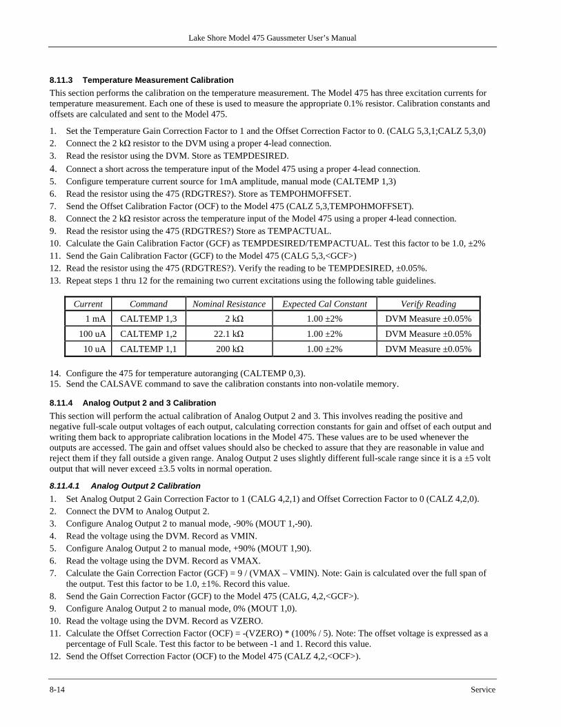
Lake Shore Model 475 Gaussmeter User’s Manual
8-14 Service
8.11.3 Temperature Measurement Calibration This section performs the calibration on the temperature measurement. The Model 475 has three excitation currents for temperature measurement. Each one of these is used to measure the appropriate 0.1% resistor. Calibration constants and offsets are calculated and sent to the Model 475.
1. Set the Temperature Gain Correction Factor to 1 and the Offset Correction Factor to 0. (CALG 5,3,1;CALZ 5,3,0) 2. Connect the 2 kΩ resistor to the DVM using a proper 4-lead connection. 3. Read the resistor using the DVM. Store as TEMPDESIRED. 4. Connect a short across the temperature input of the Model 475 using a proper 4-lead connection. 5. Configure temperature current source for 1mA amplitude, manual mode (CALTEMP 1,3) 6. Read the resistor using the 475 (RDGTRES?). Store as TEMPOHMOFFSET. 7. Send the Offset Calibration Factor (OCF) to the Model 475 (CALZ 5,3,TEMPOHMOFFSET). 8. Connect the 2 kΩ resistor across the temperature input of the Model 475 using a proper 4-lead connection. 9. Read the resistor using the 475 (RDGTRES?) Store as TEMPACTUAL. 10. Calculate the Gain Calibration Factor (GCF) as TEMPDESIRED/TEMPACTUAL. Test this factor to be 1.0, ±2% 11. Send the Gain Calibration Factor (GCF) to the Model 475 (CALG 5,3,<GCF>) 12. Read the resistor using the 475 (RDGTRES?). Verify the reading to be TEMPDESIRED, ±0.05%. 13. Repeat steps 1 thru 12 for the remaining two current excitations using the following table guidelines.
Current Command Nominal Resistance Expected Cal Constant Verify Reading 1 mA CALTEMP 1,3 2 kΩ 1.00 ±2% DVM Measure ±0.05%
100 uA CALTEMP 1,2 22.1 kΩ 1.00 ±2% DVM Measure ±0.05% 10 uA CALTEMP 1,1 200 kΩ 1.00 ±2% DVM Measure ±0.05%
14. Configure the 475 for temperature autoranging (CALTEMP 0,3). 15. Send the CALSAVE command to save the calibration constants into non-volatile memory.
8.11.4 Analog Output 2 and 3 Calibration This section will perform the actual calibration of Analog Output 2 and 3. This involves reading the positive and negative full-scale output voltages of each output, calculating correction constants for gain and offset of each output and writing them back to appropriate calibration locations in the Model 475. These values are to be used whenever the outputs are accessed. The gain and offset values should also be checked to assure that they are reasonable in value and reject them if they fall outside a given range. Analog Output 2 uses slightly different full-scale range since it is a ±5 volt output that will never exceed ±3.5 volts in normal operation.
8.11.4.1 Analog Output 2 Calibration 1. Set Analog Output 2 Gain Correction Factor to 1 (CALG 4,2,1) and Offset Correction Factor to 0 (CALZ 4,2,0). 2. Connect the DVM to Analog Output 2. 3. Configure Analog Output 2 to manual mode, -90% (MOUT 1,-90). 4. Read the voltage using the DVM. Record as VMIN. 5. Configure Analog Output 2 to manual mode, +90% (MOUT 1,90). 6. Read the voltage using the DVM. Record as VMAX. 7. Calculate the Gain Correction Factor (GCF) = 9 / (VMAX – VMIN). Note: Gain is calculated over the full span of
the output. Test this factor to be 1.0, ±1%. Record this value. 8. Send the Gain Correction Factor (GCF) to the Model 475 (CALG, 4,2,<GCF>). 9. Configure Analog Output 2 to manual mode, 0% (MOUT 1,0). 10. Read the voltage using the DVM. Record as VZERO. 11. Calculate the Offset Correction Factor (OCF) = -(VZERO) * (100% / 5). Note: The offset voltage is expressed as a
percentage of Full Scale. Test this factor to be between -1 and 1. Record this value. 12. Send the Offset Correction Factor (OCF) to the Model 475 (CALZ 4,2,<OCF>).
Lake Shore Model 475 Gaussmeter User’s Manual
Service 8-15
13. Configure Analog Output 2 to manual mode, -50% (MOUT 1,-50). 14. Read the voltage using the DVM. Verify the reading to be –2.5 VDC, ±1 mV. Record the reading. 15. Configure Analog Output 2 to manual mode, +50% (MOUT 1,50). 16. Read the voltage using the DVM. Verify the reading to be +2.5 VDC, ±1 mV. Record the reading. 17. Configure Analog Output 2 to manual mode, 0% (MOUT 1,0). 18. Read the voltage using the DVM. Verify the reading to be 0 VDC, ±1 mV. Record the reading. 19. Send the CALSAVE command to save the calibration constants into non-volatile memory.
8.11.4.2 Analog Output 3 Calibration 1. Set Analog Output 3 Gain Correction Factor to 1 (CALG 4,3,1) and Offset Correction Factor to 0 (CALZ 4,3,0). 2. Connect the DVM to Analog Output 3. 3. Configure Analog Output 3 to manual mode, -100% (ANALOG 3,2,0,0,-100,10). 4. Read the voltage using the DVM. Record as VMIN. 5. Configure Analog Output 3 to manual mode, +100% (ANALOG 3,2,0,0,100,10). 6. Read the voltage using the DVM. Record as VMAX. 7. Calculate the Gain Correction Factor (GCF) = 20 / (VMAX – VMIN). Note: Gain is calculated over the full span of
the output. Test this factor to be 1.0, ±1%. Record this value. 8. Send the Gain Correction Factor (GCF) to the Model 475 (CALG, 4,3,<GCF>). 9. Configure Analog Output 3 to manual mode, 0% (ANALOG 3,2,0,0,0,10). 10. Read the voltage using the DVM. Record as VZERO. 11. Calculate the Offset Correction Factor (OCF) = -(VZERO) * (100% / 10). Note: The offset voltage is expressed as a
percentage of Full Scale. Test this factor to be between -1 and 1. Record this value. 12. Send the Offset Correction Factor (OCF) to the Model 475 (CALZ 4,3,<OCF>). 13. Configure Analog Output 3 to manual mode, -100% (ANALOG 3,2,0,0,-100,10). 14. Read the voltage using the DVM. Verify the reading to be –10 VDC, ±1 mV. Record the reading. 15. Configure Analog Output 3 to manual mode, +100% (ANALOG 3,2,0,0,100,10). 16. Read the voltage using the DVM. Verify the reading to be +10 VDC, ±1 mV. Record the reading. 17. Configure Analog Output 3 to manual mode, 0% (ANALOG 3,2,0,0,0,10). 18. Read the voltage using the DVM. Verify the reading to be 0 VDC, ±1 mV. Record the reading. 19. Send the CALSAVE command to save the calibration constants into non-volatile memory.
Lake Shore Model 475 Gaussmeter User’s Manual
8-16 Service
8.11.5 Calibration Specific Interface Commands
CALG Gain Calibration Constant Command Input: CALG <type>, <range>, <value>[term] Format: n,n,±nnnnnnn
<type> Specifies the item to calibrate. Valid entries are: 1 = 100 mA hall current source 2 = 10 mA hall current source 3 = 1 mA hall current source 4 = Analog Outputs (1-3) 5 = Temperature
<range> Specifies the range of the item to calibrate. Valid entries are: 1 = 300 μΩ range (hall current source), 10 μA range (temperature), Analog Output 1 (not used) 2 = 3 mΩ range (hall current source), 100 μA range (temperature), Analog Output 2 3 = 30 mΩ range (hall current source), 1 mA range (temperature), Analog Output 3 4 = 300 mΩ range (hall current source) 5 = 3 Ω range (hall current source)
<value> Gain calibration constant value. Remarks: Some entries are not calibrated and are indicated by “not used.” No value should be sent to these
locations.
CALG? Gain Calibration Constant Query Input: CALG? <type>,<range> [term]
Format: n,n <type> 1 – 5 <range> 1 – 5
Returned: <value>[term] Format: ±nnnnnnn (Refer to command for description)
CALSAVE Calibration Save Command Input: CALSAVE [term] Remarks: Saves all CALZ and CALG calibration constants in non-volatile memory.
CALTEMP Temperature Measurement Setup Command Input: CALTEMP <mode>, <range>[term] Format: n,n
<mode> Specifies the operating mode of the temperature measurement. Valid entries are: 0 = Normal mode, autorange on 1 = Manual range mode
<range> Specifies the current source range of the temperature measurement. Valid entries are: 1 = 10 μA range (250 kΩ range) 2 = 100 μA range (25 kΩ range) 3 = 1 mA range (2.5 kΩ range)
Remarks: This command is used to set the temperature measurement to manual mode so that each range can be calibrated. Default is mode = 0 (autorange).
CALTEMP? Temperature Measurement Setup Query Input: CALTEMP? [term] Returned: <mode>, <range>[term]
Format: n,n (Refer to command for description)
Lake Shore Model 475 Gaussmeter User’s Manual
Service 8-17
CALZ Zero Offset Calibration Constant Command Input: CALZ <type>, <range>, <value>[term] Format: n,n,±nnnnnnn
<type> Specifies the item to calibrate. Valid entries are: 1 = 100 mA hall current source (not used) 2 = 10 mA hall current source (not used) 3 = 1 mA hall current source (not used) 4 = Analog Outputs (1-3) 5 = Temperature
<range> Specifies the range of the item to calibrate. Valid entries are: 1 = 300 μΩ range (hall current source, not used), 10 μA range (temp.), Analog Output 1 (not used) 2 = 3 mΩ range (hall current source, not used), 100 μA range (temp.), Analog Output 2 3 = 30 mΩ range (hall current source, not used), 1 mA range (temp.), Analog Output 3 4 = 300 mΩ range (hall current source, not used) 5 = 3 Ω range (hall current source, not used)
<value> Zero offset calibration constant value. Remarks: The range variable is ignored but needs to be sent for types that do not need to specify a range (types 2,
3, and 4). A range value of 1 should be sent for those types. The hall current sources do not have a calibrated zero. The offset is corrected using the Zero Probe function.
CALZ? Zero Offset Calibration Constant Query Input: CALZ? <type>, <range>[term]
Format: n,n <input> 1 – 5 <type> 1 – 5
Returned: <value>[term] Format: ±nnnnnnn (Refer to command for description)
CSMODE Hall Current Source Mode Command Input: CSMODE <mode> [term] Format: n
<mode> Specifies the hall current source mode. Valid entries are: 0 = Current off 1 = Normal mode (current reversal) 2 = Positive current 3 = Negative current
Remarks: Configures the hall current source mode. The current output (100 mA, 10 mA, or 1mA) is dependent on range (see HALLCS).
CSMODE? Hall Current Source Mode Query Input: CSMODE? [term] Returned: <mode>[term]
Format: n (Refer to command for description)
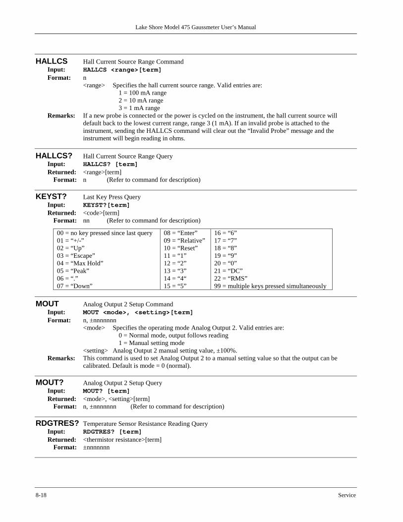
Lake Shore Model 475 Gaussmeter User’s Manual
8-18 Service
HALLCS Hall Current Source Range Command Input: HALLCS <range>[term] Format: n
<range> Specifies the hall current source range. Valid entries are: 1 = 100 mA range 2 = 10 mA range 3 = 1 mA range
Remarks: If a new probe is connected or the power is cycled on the instrument, the hall current source will default back to the lowest current range, range 3 (1 mA). If an invalid probe is attached to the instrument, sending the HALLCS command will clear out the “Invalid Probe” message and the instrument will begin reading in ohms.
HALLCS? Hall Current Source Range Query Input: HALLCS? [term] Returned: <range>[term]
Format: n (Refer to command for description)
KEYST? Last Key Press Query Input: KEYST?[term] Returned: <code>[term]
Format: nn (Refer to command for description)
00 = no key pressed since last query 01 = “+/-” 02 = “Up” 03 = “Escape” 04 = “Max Hold” 05 = “Peak” 06 = “.” 07 = “Down”
08 = “Enter” 09 = “Relative” 10 = “Reset” 11 = “1” 12 = “2” 13 = “3” 14 = “4“ 15 = “5”
16 = “6” 17 = “7” 18 = “8” 19 = “9” 20 = “0” 21 = “DC” 22 = “RMS” 99 = multiple keys pressed simultaneously
MOUT Analog Output 2 Setup Command Input: MOUT <mode>, <setting>[term] Format: n, ±nnnnnnn
<mode> Specifies the operating mode Analog Output 2. Valid entries are: 0 = Normal mode, output follows reading 1 = Manual setting mode
<setting> Analog Output 2 manual setting value, ±100%. Remarks: This command is used to set Analog Output 2 to a manual setting value so that the output can be
calibrated. Default is mode = 0 (normal).
MOUT? Analog Output 2 Setup Query Input: MOUT? [term] Returned: <mode>, <setting>[term]
Format: n, ±nnnnnnn (Refer to command for description)
RDGTRES? Temperature Sensor Resistance Reading Query Input: RDGTRES? [term] Returned: <thermistor resistance>[term]
Format: ±nnnnnnn
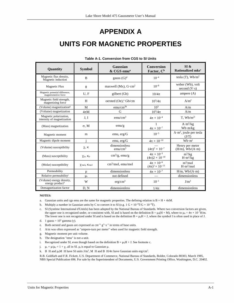
Lake Shore Model 475 Gaussmeter User’s Manual
Units for Magnetic Properties A-1
APPENDIX A
UNITS FOR MAGNETIC PROPERTIES
Table A-1. Conversion from CGS to SI Units
Quantity Symbol Gaussian & CGS emua
Conversion Factor, Cb
SI & Rationalized mksc
Magnetic flux density, Magnetic induction B gauss (G)d 10–4 tesla (T), Wb/m2
Magnetic Flux φ maxwell (Mx), G·cm2 10–8 weber (Wb), volt second (V·s)
Magnetic potential difference, magnetomotive force U, F gilbert (Gb) 10/4π ampere (A)
Magnetic field strength, magnetizing force H oersted (Oe),e Gb/cm 103/4π A/mf
(Volume) magnetizationg M emu/cm3h 103 A/m (Volume) magnetization 4πM G 103/4π A/m Magnetic polarization,
intensity of magnetization J, I emu/cm3 4π × 10–4 T, Wb/m2i
(Mass) magnetization σ, M emu/g 1 4π × 10–7
A·m2/kg Wb·m/kg
Magnetic moment m emu, erg/G 10–3 A·m2, joule per tesla (J/T)
Magnetic dipole moment j emu, erg/G 4π × 10–10 Wb·mi
(Volume) susceptibility χ, κ dimensionless emu/cm3
— (4π)2 × 10⁻⁷
Henry per meter (H/m), Wb/(A·m)
(Mass) susceptibility χρ, κρ cm3/g, emu/g 4π × 10–3 (4π)2 × 10⁻¹⁰
m3/kg H·m2/kg
(Molar) susceptibility χmol, κmol cm3/mol, emu/mol 4π × 10–6 (4π)2 × 10–13
m3/mol H·m2/mol
Permeability µ dimensionless 4π × 10–7 H/m, Wb/(A·m) Relative permeabilityj µr not defined — dimensionless
(Volume) energy density, energy productk W erg/cm3 10–1 J/m3
Demagnetization factor D, N dimensionless 1/4π dimensionless
NOTES: a. Gaussian units and cgs emu are the same for magnetic properties. The defining relation is B = H + 4πM. b. Multiply a number in Gaussian units by C to convert it to SI (e.g. 1 G × 10–4T/G = 10–4T). c. SI (Système International d'Unités) has been adopted by the National Bureau of Standards. Where two conversion factors are given,
the upper one is recognized under, or consistent with, SI and is based on the definition B = µ0(H + M), where to µ0 = 4π × 10–7H/m. The lower one is not recognized under SI and is based on the definition B = µ0H + J, where the symbol I is often used in place of J.
d. 1 gauss = 105 gamma (γ). e. Both oersted and gauss are expressed as cm–½ g½·s–1 in terms of base units. f. A/m was often expressed as "ampere-turn per meter" when used for magnetic field strength. g. Magnetic moment per unit volume. h. The designation "emu" is not a unit. i. Recognized under SI, even though based on the definition B = µ0H + J. See footnote c. j. µr = µ/µ0 = 1 + χ, all in SI. µr is equal to Gaussian µ. k. B H and µ0M H have SI units J/m3, M H and B H/4π have Gaussian units erg/cm3. R.B. Goldfarb and F.R. Fickett, U.S. Department of Commerce, National Bureau of Standards, Bolder, Colorado 80303, March 1985, NBS Special Publication 696. For sale by the Superintendent of Documents, U.S. Government Printing Office, Washington, D.C. 20402.
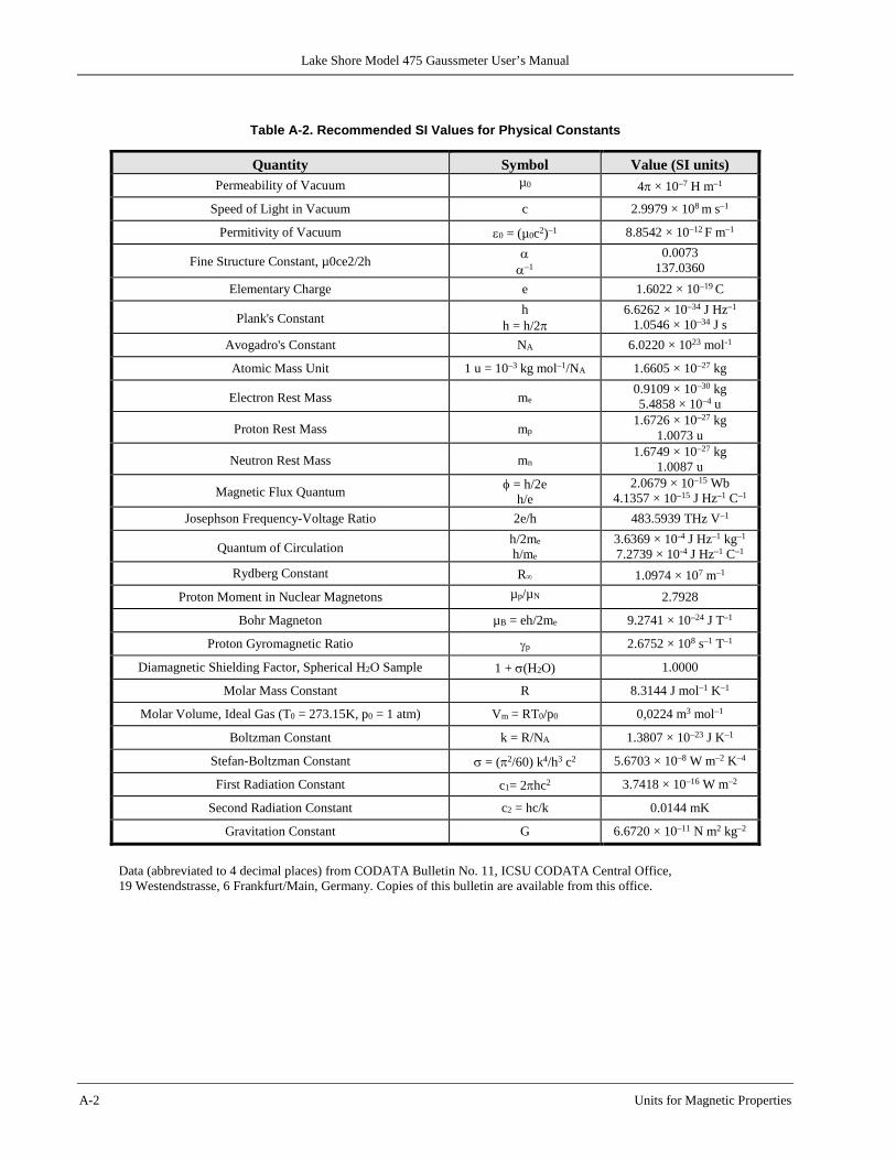
Lake Shore Model 475 Gaussmeter User’s Manual
A-2 Units for Magnetic Properties
Table A-2. Recommended SI Values for Physical Constants
Quantity Symbol Value (SI units) Permeability of Vacuum µ0 4π × 10–7 H m–1
Speed of Light in Vacuum c 2.9979 × 10⁸ m s–1
Permitivity of Vacuum ε0 = (µ0c2)–1 8.8542 × 10⁻¹² F m–1
Fine Structure Constant, µ0ce2/2h α α–1
0.0073 137.0360
Elementary Charge e 1.6022 × 10⁻¹⁹ C
Plank's Constant h
h = h/2π 6.6262 × 10⁻³⁴ J Hz–1
1.0546 × 10⁻³⁴ J s Avogadro's Constant NA 6.0220 × 10²³ mol-1
Atomic Mass Unit 1 u = 10–3 kg mol–1/NA 1.6605 × 10⁻²⁷ kg
Electron Rest Mass me 0.9109 × 10⁻³⁰ kg 5.4858 × 10⁻⁴ u
Proton Rest Mass mp 1.6726 × 10⁻²⁷ kg
1.0073 u
Neutron Rest Mass mn 1.6749 × 10⁻²⁷ kg
1.0087 u
Magnetic Flux Quantum φ = h/2e h/e
2.0679 × 10⁻¹⁵ Wb 4.1357 × 10⁻¹⁵ J Hz–1 C–1
Josephson Frequency-Voltage Ratio 2e/h 483.5939 THz V–1
Quantum of Circulation h/2me h/me
3.6369 × 10⁻⁴ J Hz–1 kg–1 7.2739 × 10⁻⁴ J Hz–1 C–1
Rydberg Constant R∞ 1.0974 × 10⁷ m–1 Proton Moment in Nuclear Magnetons µp/µN 2.7928
Bohr Magneton µB = eh/2me 9.2741 × 10⁻²⁴ J T–1
Proton Gyromagnetic Ratio γp 2.6752 × 10⁸ s–1 T–1
Diamagnetic Shielding Factor, Spherical H2O Sample 1 + σ(H2O) 1.0000
Molar Mass Constant R 8.3144 J mol–1 K–1
Molar Volume, Ideal Gas (T0 = 273.15K, p0 = 1 atm) Vm = RT0/p0 0,0224 m3 mol–1
Boltzman Constant k = R/NA 1.3807 × 10⁻²³ J K–1
Stefan-Boltzman Constant σ = (π2/60) k4/h3 c2 5.6703 × 10⁻⁸ W m–2 K–4
First Radiation Constant c1= 2πhc2 3.7418 × 10⁻¹⁶ W m–2
Second Radiation Constant c2 = hc/k 0.0144 mK
Gravitation Constant G 6.6720 × 10⁻¹¹ N m2 kg–2
Data (abbreviated to 4 decimal places) from CODATA Bulletin No. 11, ICSU CODATA Central Office, 19 Westendstrasse, 6 Frankfurt/Main, Germany. Copies of this bulletin are available from this office.