L -THEORY FOR THE BOUSSINESQ SYSTEM PAUL ANDR ES …

UNIVERSIDAD DE CHILEFACULTAD DE CIENCIAS FISICAS Y MATEMATICASDEPARTAMENTO DE INGENIERIA MATEMATICA

Lp-THEORY FOR THE BOUSSINESQ SYSTEM

TESIS PARA OPTAR AL GRADO DE DOCTOR EN CIENCIAS DE LAINGENIERIA, MENCION MODELACION MATEMATICA

EN COTUTELA CON LA UNIVERSITE DE PAU ET DES PAYS DE L’ADOUR

PAUL ANDRES ACEVEDO TAPIA

PROFESOR GUIA 1:CARLOS CONCA ROSENDE

PROFESOR GUIA 2:CHERIF AMROUCHE

MIEMBROS DE LA COMISION:MARIA ELENA SCHONBEK

MARKO ROJAS MEDARMARC DAMBRINE

AXEL OSSES ALVARADORAFAEL BENGURIA DONOSO

MARIO DURAN TORO

SANTIAGO DE CHILE2015

SUMMARY OF THE THESIS TO OBTAINTHE DEGREE OF: Doctor en Ciencias de laIngeniería, Mención Modelación MatemáticaBY: Paul Andrés Acevedo TapiaDATE: September 16th, 2015ADVISOR 1: Carlos Conca RosendeADVISOR 2: Chérif Amrouche

Lp-THEORY FOR THE BOUSSINESQ SYSTEM

This thesis is dedicated to the study of the stationary Boussinesq system:

−ν∆u+ (u · ∇)u+∇π = θg in Ω, div u = 0 in Ω, (0.1a)

−κ∆θ + u · ∇θ = h in Ω, (0.1b)

where Ω ⊂ R3 is an open bounded connected set; u, π and θ are the velocity field, pressureand temperature of the fluid, respectively, and stand for the unknowns of the system; ν > 0is the kinematic viscosity of the fluid, κ > 0 is the thermal diffusivity of the fluid, g is thegravitational acceleration and h is a heat source applied to the fluid.

The aim of this thesis is the study of the Lp-theory for the stationary Boussinesq systemin the context of two different types of boundary conditions for the velocity field. Indeed, inthe first part of the thesis, we will consider a non-homogeneous Dirichlet boundary condition

u = ub on Γ, (0.2)

where Γ denotes the boundary of the domain; meanwhile in the second part, the velocityfield will be prescribed through a non-homogeneous Navier boundary condition

u · n = 0, 2 [D(u)n]τ + α uτ = a, on Γ, (0.3)

where D(u) = 12

(∇u+ (∇u)T

)is the strain tensor associated with the velocity field u, n

is the unit outward normal vector, τ is the corresponding unit tangent vector, α and aare a friction scalar function and a tangential vector field defined both on the boundary,respectively. Further, the boundary condition for the temperature will be, in the first twoparts of the thesis, a non-homogeneous Dirichlet boundary condition

θ = θb on Γ. (0.4)

Then, firstly, we study the existence and uniqueness of the weak solution for the problem(0.1), (0.2) and (0.4) in the hilbertian case. Also, the existence of generalized solutions forp ≥ 3

2and strong solutions for 1 < p < ∞ is showed. Furthermore, the existence and

uniqueness of the very weak solution is studied. It is worth to note that because a non-homogeneous Dirichlet boundary condition is considered for the velocity field, the fact thatthe boundary of the domain could be non-connected plays a fundamental role since it appearsin an explicit way in the assumptions of some of the main results.

In the second part, we study the existence of weak solutions in the Hilbert case, as well asthe existence of generalized solutions for p > 2 and strong solutions for p ≥ 6

5for the problem

(0.1), (0.3) and (0.4). Note that the assumption of a non-connected boundary, which wasmentioned before, will not appear here due to the impermeability restriction on the boundary.

Finally, in the last part of this thesis, we study the Lp-theory for the Stokes equationswith Navier boundary condition (0.3). Specifically, we deal with theW 1,p-regularity for p ≥ 2and the W 2,p-regularity for p ≥ 6

5.

i

RÉSUMÉ DE LA THÈSE POUR OBTENIRLE DEGRE DE: Doctor en Ciencias de laIngeniería, Mención Modelación MatemáticaPAR: Paul Andrés Acevedo TapiaDATE: 16 Septembre 2015DIRECTEUR DE THÈSE 1: Carlos Conca RosendeDIRECTEUR DE THÈSE 2: Chérif Amrouche

THÉORIE Lp POUR LE SYSTÈME DE BOUSSINESQ

Cette thèse est consacrée à l’étude du système de Boussinesq stationnaire:

−ν∆u+ (u · ∇)u+∇π = θg dans Ω, div u = 0 dans Ω, (0.1a)

−κ∆θ + u · ∇θ = h dans Ω, (0.1b)

où Ω ⊂ R3 est un ouvert, borné et connexe; les inconnues du système sont u, π et θ: la vitesse,la pression et la température du fluide, respectivement; ν > 0 est la viscosité cinématique dufluide, κ > 0 est la diffusivité thermique du fluide, g est l’accélération de la pesanteur et hest une source de chaleur appliquée au fluide.

L’objectif de cette thèse est l’étude de la théorie Lp pour le système de Boussinesq enconsidérant deux différents types de conditions aux limites du champ de vitesse. En effet,dans une premierè partie, nous considérons une condition de Dirichlet non homogène

u = ub sur Γ, (0.2)

où Γ désigne la frontière du domaine. Dans une deuxième partie, nous considéron unecondition de Navier non homogène

u · n = 0, 2 [D(u)n]τ + α uτ = a, sur Γ, (0.3)

où D(u) = 12

(∇u+ (∇u)T

)est le tenseur de déformation associé au champ de vitesse u, n

est le vecteur normal unitaire extérieur, τ est le correspondant vecteur tangent unitaire, αet a sont une fonction scalaire de friction et un champ de vecteur tangentiel donnés sur lafrontière, respectivement. De plus, la condition aux limites pour la température sera, dansles deux premières parties, une condition aux limites de Dirichlet non homogène

θ = θb sur Γ. (0.4)

Alors, premièrement, nous étudions l’existence et l’unicité d’une solution faible pour le prob-lème (0.1), (0.2) et (0.4) dans le cas hilbertien. Également, l’existence de solutions général-isées pour p ≥ 3

2et des solutions fortes pour 1 < p <∞ est démontrée. De plus, l’existence

et l’unicité de la solution très faible sont étudiés. Il est intéressant de noter que puisqueune condition de Dirichlet non homogène est considérée pour le champ de vitesse, le faitque la frontière du domaine pourrait être non-connexe joue un rôle fondamental puisque celaapparait de manière explicite dans les hypothèses des principaux résultats.

D’autre part, dans la deuxième partie, nous étudions l’existence de solutions faibles dansle cas hilbertien, ainsi que l’existence de solutions généralisées pour p > 2 et des solutionsfortes pour p ≥ 6

5pour le problème (0.1), (0.3) et (0.4). Notez que l’hypothèse d’une frontière

non-connexe, mentionnée précédemment, ne figurait pas dans cette partie du travail en raisonde la restriction d’imperméabilité de la frontière.

Enfin, dans la dernière partie de cette thèse, nous étudions la théorie Lp pour les équationsde Stokes avec la condition de Navier (0.3). Plus précisément, nous examinons la régularitéW 1,p pour p ≥ 2 et la régularité W 2,p pour p ≥ 6

5.

ii

RESUMEN DE LA TESIS PARA OPTAREL GRADO DE: Doctor en Ciencias de laIngeniería, Mención Modelación MatemáticaPOR: Paul Andrés Acevedo TapiaFECHA: 16 de Septiembre de 2015PROFESOR GUÍA 1: Carlos Conca RosendePROFESOR GUÍA 2: Chérif Amrouche

TEORÍA Lp PARA EL SISTEMA DE BOUSSINESQ

Esta tesis está dedicada al estudio del sistema de Boussinesq estacionario:

−ν∆u+ (u · ∇)u+∇π = θg en Ω, div u = 0 en Ω, (0.1a)

−κ∆θ + u · ∇θ = h en Ω, (0.1b)donde Ω ⊂ R3 es un conjunto abierto, acotado y conexo; u, π y θ representan el campode velocidades, la presión y la temperatura del fluido, respectivamente, siendo éstas lasincógnitas del sistema; ν > 0 es la viscosidad cinemática del fluido, κ > 0 es la difusividadtérmica del fluido, g es la aceleración de la gravedad y h es una fuente de calor aplicada alfluido.

El objetivo de esta tesis es el estudio de la teoría Lp para el sistema de Boussinesq esta-cionario considerando dos diferentes tipos de condiciones de frontera del campo de veloci-dades. En efecto, en una primera etapa, se considerará la condición de frontera de Dirichletno homogéneo

u = ub sobre Γ, (0.2)donde Γ denota la frontera del dominio; mientras que en una segunda etapa, el campo develocidades tendrá prescrito la condición de frontera de Navier no homogéneo

u · n = 0, 2 [D(u)n]τ + α uτ = a, sobre Γ, (0.3)

donde D(u) = 12

(∇u+ (∇u)T

)es el tensor de deformación asociado con el campo de ve-

locidades u, n es el vector normal unitario exterior, τ es el correspondiente vector unitariotangente, α y a son una función de fricción y un campo vectorial tangencial definidas ambassobre la frontera. Además, la condición de frontera para la temperatura será, en las dosprimeras partes, la condición de frontera de Dirichlet no homogéneo

θ = θb sobre Γ. (0.4)

Así, en primer lugar, estudiamos la existencia y unicidad de la solución débil para el problema(0.1), (0.2) y (0.4) en el caso hilbertiano. Además, la existencia de soluciones generalizadaspara p ≥ 3

2y soluciones fuertes para 1 < p < ∞ es probada. También, se estudiará la

existencia y unicidad de la solución muy débil. Vale la pena señalar que debido a que lacondición de Dirichlet no homogénea es considerada para la velocidad, el hecho de que lafrontera del dominio pueda ser no conexa juega un papel importante, ya que aparece demanera explícita en las hipótesis de algunos de los principales resultados.

Por otro lado, en la segunda etapa de la tesis, se estudiará la existencia de solucionesdébiles en el caso de Hilbert, así como la existencia de soluciones generalizadas para p > 2 ysoluciones fuertes para p ≥ 6

5para el problema (0.1), (0.3) y (0.4). Tenga en cuenta que la

suposición hecha anteriormente acerca de la no conexidad de la frontera no aparecerá aquídebido a la restricción de impermeabilidad en la frontera.

Finalmente, en la última parte de esta tesis, estudiamos la teoría Lp para las ecuaciones deStokes con la condición de Navier (0.3). Más precisamente, nos ocuparemos de la regularidadW 1,p para p ≥ 2 y la regularidad W 2,p para p ≥ 6

5.

iii

To my little inspiring twins Giuly and Nicky, and to my parents Ángel Guido and NancyBeatriz who have been a very important support in my life

iv

Acknowledgements

This thesis would not have been possible without the invaluable guidance of my advisorsProf. Carlos Conca (University of Chile, UChile) and Prof. Chérif Amrouche (Universitéde Pau et des Pays de l’Adour, France, UPPA). I am very grateful to both of them for allthe opportunities that we had to discuss Mathematics, for their helpful advices and for theircomplete support in my PhD studies. There is no doubt that it has been a great honor forme to have worked with Carlos and Chérif, two fantastic mathematicians, researchers andexcellent people.

I want to thank Prof. María Elena Schonbek (University of California, Santa Cruz -USA) for her excellent disposition to read this thesis and for her great suggestions andremarks which served to improve the redaction of the thesis; as well as I would like to thankProf. Marko Rojas-Medar (University of Bío-Bío, Chile) for dedicating his time to review thiswork. Also, I would like to express my sincere gratitude to Prof. Marc Dambrine (UPPA),Prof. Axel Osses (UChile), Prof. Rafael Benguria (Pontificia Universidad Católica de Chile,PUC) and Prof. Mario Durán (PUC) for accepting to be part of my graduate committee.

My sincere thanks also goes to Prof. Jacques Giacomoni who provided me the opportunityand the facilities to visit the “Laboratoire De Mathématiques et de leurs Applications de Pau”(LMAP - UPPA). Of course this experience was undoubtedly very important for my life andfor my integral formation as a researcher.

I am very grateful for the important financial support that I received from the CMM(Center for Mathematical Modeling - UChile), with the approbation of the director Prof.Alejandro Jofré, during all my PhD studies. Also, my gratitude to LMAP, directed by Prof.Jacques Giacomoni, for the funding that they gave me in my stay in the warm and prettycity of Pau.

I would need more than one page (with the risk of not considering all of them) to list allthe people who helped me in some manner during my stay in Santiago and Pau. For thatreason I would like to thank to every person of the administrative staff from the Departmentof Mathematical Engineering (DIM) at the UChile, CMM, Postgraduate School of the Facultyof Physics and Mathematics Sciences (FCFM) at the UChile, LMAP, Ecole Doctorale DesSciences Exactes Et Leurs Applications (ED SEA) at the UPPA and the CLOUS at theUPPA, for all their good disposition each time when I needed them. A special gratitude toMrs. Georgina for her incredible sense of humor, her invaluable help and her great labor inthe DIM.

In the same way as before I want to express my gratitude to every partner that I metduring all my studies in the UChile and UPPA. All of them have contributed to do my stayin Santiago and Pau very pleasant.

Last but not least, I would like to thank my family, specially my parents who have beenan important support in many aspects of my life, and of course to my lovely and beautifulgirls who in their innocence have supported me despite the distance.

Paul

v

Contents

List of Figures vii

1 General Introduction 11.1 Preliminaries . . . . . . . . . . . . . . . . . . . . . . . . . . . . . . . . . . . 11.2 Thesis Description and Main Results . . . . . . . . . . . . . . . . . . . . . . 8

1.2.1 Boussinesq system with Dirichlet boundary conditions for the velocityfield . . . . . . . . . . . . . . . . . . . . . . . . . . . . . . . . . . . . 9

1.2.2 Boussinesq system with Navier boundary conditions for the velocity field 111.2.3 Stokes equations with Navier boundary condition . . . . . . . . . . . 12

2 Boussinesq system with Dirichlet boundary conditions 142.1 Introduction . . . . . . . . . . . . . . . . . . . . . . . . . . . . . . . . . . . . 142.2 Main results . . . . . . . . . . . . . . . . . . . . . . . . . . . . . . . . . . . . 172.3 Notations and some useful results . . . . . . . . . . . . . . . . . . . . . . . . 202.4 Weak solutions . . . . . . . . . . . . . . . . . . . . . . . . . . . . . . . . . . 252.5 Regularity of the weak solution . . . . . . . . . . . . . . . . . . . . . . . . . 312.6 Very weak solutions . . . . . . . . . . . . . . . . . . . . . . . . . . . . . . . . 332.7 Estimates and uniqueness of the weak solution . . . . . . . . . . . . . . . . . 56

3 Boussinesq system with Navier boundary conditions 623.1 Introduction . . . . . . . . . . . . . . . . . . . . . . . . . . . . . . . . . . . . 623.2 Main results . . . . . . . . . . . . . . . . . . . . . . . . . . . . . . . . . . . . 643.3 Notations and some useful results . . . . . . . . . . . . . . . . . . . . . . . . 653.4 Weak solutions . . . . . . . . . . . . . . . . . . . . . . . . . . . . . . . . . . 723.5 Regularity of the weak solution . . . . . . . . . . . . . . . . . . . . . . . . . 78

4 Stokes equations with Navier boundary condition 814.1 Introduction . . . . . . . . . . . . . . . . . . . . . . . . . . . . . . . . . . . . 814.2 Main results . . . . . . . . . . . . . . . . . . . . . . . . . . . . . . . . . . . . 814.3 Notations and some useful results . . . . . . . . . . . . . . . . . . . . . . . . 824.4 Weak solution in the Hilbert case . . . . . . . . . . . . . . . . . . . . . . . . 864.5 Regularity of the weak solution . . . . . . . . . . . . . . . . . . . . . . . . . 89

Bibliography 92

vi

List of Figures

1.1 Joseph Boussinesq . . . . . . . . . . . . . . . . . . . . . . . . . . . . . . . . 11.2 Convection currents . . . . . . . . . . . . . . . . . . . . . . . . . . . . . . . . 41.3 Lord Rayleigh . . . . . . . . . . . . . . . . . . . . . . . . . . . . . . . . . . . 51.4 Henri Bénard . . . . . . . . . . . . . . . . . . . . . . . . . . . . . . . . . . . 51.5 Bénard cells . . . . . . . . . . . . . . . . . . . . . . . . . . . . . . . . . . . . 51.6 Mantle currents . . . . . . . . . . . . . . . . . . . . . . . . . . . . . . . . . . 61.7 Interface between two mediums . . . . . . . . . . . . . . . . . . . . . . . . . 71.8 Solid-liquid interface . . . . . . . . . . . . . . . . . . . . . . . . . . . . . . . 71.9 Velocity profiles of fluid flow . . . . . . . . . . . . . . . . . . . . . . . . . . . 7

vii

Chapter 1

General Introduction

1.1 PreliminariesThis thesis is concerned with the study of the following stationary Boussinesq system:

−ν∆u+ (u · ∇)u+∇π = θg in Ω, div u = 0 in Ω, (1.1a)

−κ∆θ + u · ∇θ = h in Ω, (1.1b)

where Ω ⊂ R3 is an open bounded connected set; u, π and θ are the velocity field, pressureand temperature of the fluid, respectively, and stand for the unknowns of the system; ν > 0is the kinematic viscosity of the fluid, κ > 0 is the thermal diffusivity of the fluid, g is thegravitational acceleration and h is a heat source applied to the fluid.

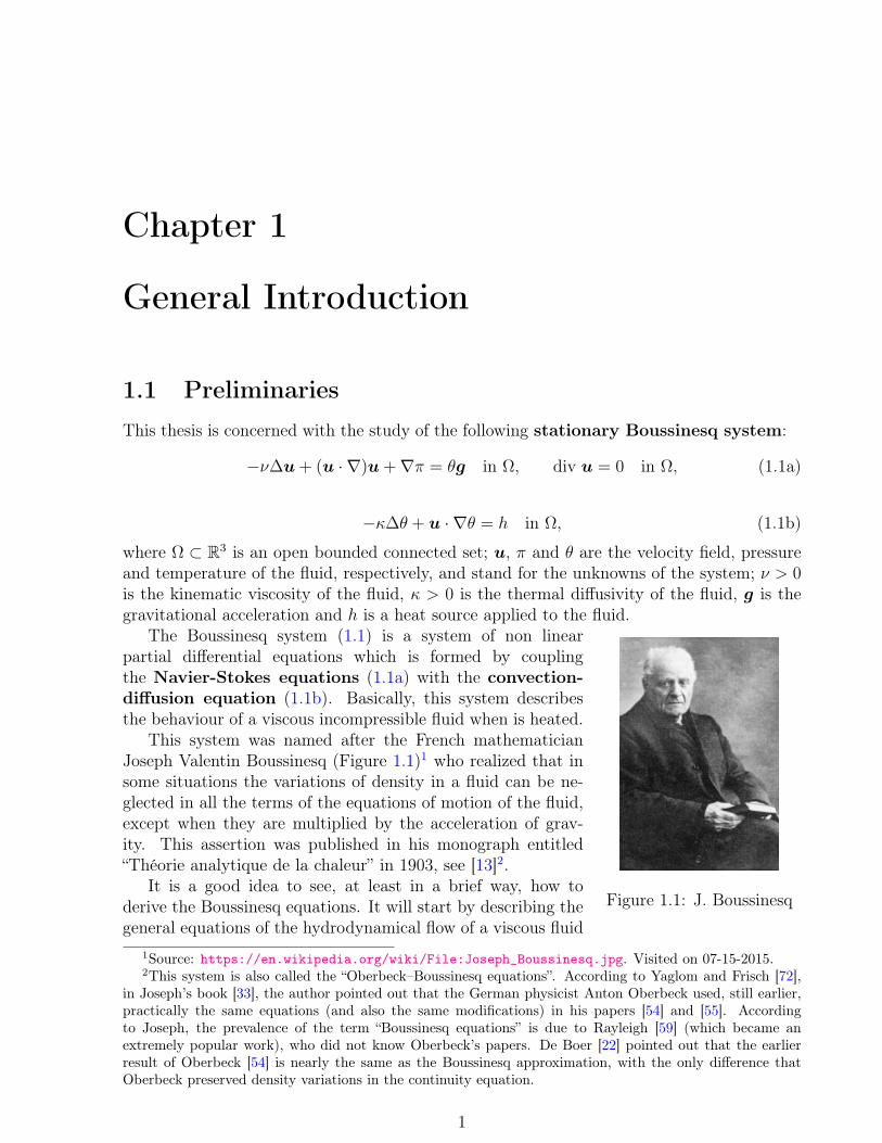
Figure 1.1: J. Boussinesq

The Boussinesq system (1.1) is a system of non linearpartial differential equations which is formed by couplingthe Navier-Stokes equations (1.1a) with the convection-diffusion equation (1.1b). Basically, this system describesthe behaviour of a viscous incompressible fluid when is heated.

This system was named after the French mathematicianJoseph Valentin Boussinesq (Figure 1.1)1 who realized that insome situations the variations of density in a fluid can be ne-glected in all the terms of the equations of motion of the fluid,except when they are multiplied by the acceleration of grav-ity. This assertion was published in his monograph entitled“Théorie analytique de la chaleur” in 1903, see [13]2.

It is a good idea to see, at least in a brief way, how toderive the Boussinesq equations. It will start by describing thegeneral equations of the hydrodynamical flow of a viscous fluid

1Source: https://en.wikipedia.org/wiki/File:Joseph_Boussinesq.jpg. Visited on 07-15-2015.2This system is also called the “Oberbeck–Boussinesq equations”. According to Yaglom and Frisch [72],

in Joseph’s book [33], the author pointed out that the German physicist Anton Oberbeck used, still earlier,practically the same equations (and also the same modifications) in his papers [54] and [55]. Accordingto Joseph, the prevalence of the term “Boussinesq equations” is due to Rayleigh [59] (which became anextremely popular work), who did not know Oberbeck’s papers. De Boer [22] pointed out that the earlierresult of Oberbeck [54] is nearly the same as the Boussinesq approximation, with the only difference thatOberbeck preserved density variations in the continuity equation.

1

https://en.wikipedia.org/wiki/File:Joseph_Boussinesq.jpg

Chapter 1. General Introduction

in the three dimensional space with density ρ and velocity fieldu. From the law of the conservation of mass, it follows the equation of continuity:

∂ρ

∂t+ div(ρu) = 0. (1.2)

The following equations of motion (best known as the Navier-Stokes equations) result fromthe conservation of the linear momentum:

ρDu

Dt= −ρg + div σ, (1.3)

where the differential operator D(·)Dt

stands for the material derivative[D(·)Dt

:=∂(·)∂t

+ (u · ∇)(·)],

g is the gravitational acceleration and σ is the stress tensor given by

σ = −πI3 + µ

(2D(u)− 2

3div u I3

)+ λ div u I3, (1.4)

with π the pressure, µ the coefficient of dynamic viscosity of the fluid, λ the bulk viscosity(or second viscosity), I3 the identity matrix of order 3 and D(u) = 1

2

(∇u+ (∇u)T

)the

deformation tensor (or strain tensor) associated with the velocity field u.The equation of heat conduction, which is obtained thanks to the law of conservation of

energy, is as follows:

ρDe

Dt= div(ktc∇θ)− πdiv u+ Φ, (1.5)

where e is the internal energy per unit mass of the fluid, ktc is the thermal conductivity, θ isthe temperature and Φ is the rate of viscous dissipation per unit volume of fluid defined by

Φ = 2µTr(D(u)2) +

(λ− 2

3µ

)(div u)2, (1.6)

where Tr(A) stands for the trace of the matrix A. It is known that for a fluid (gas or liquid)e = c θ, where c is the specific heat of the fluid. It is noteworthy that the quantities ρ, µ, λ,ktc, c and e are, in general, functions of the pressure π and the temperature θ.

Until this time we presented the general hydrodynamical equations for compressible heatconducting and diffusive flow of a viscous, nonhomogeneous fluid. However, as Boussinesqpointed out in [13], in many real situations, there are fluids for which the influence of pressureis unimportant and even the variation with temperature may be disregarded, except in so faras it modifies the action of gravity. For example, according to [33], in many real situations,there are fluids for which one needs to change the pressure by roughly five atmospheres toproduce the same change of density as a temperature difference of 1C. For example, it iseasier to change the density of water inside of a container by heating than by squeezing. Thisimplies that even vigorous motions of water will not introduce important buoyant forces otherthan those from temperature variations. Moreover, if the temperature varies little, thereforethe density varies little too, except in the buoyancy which drives the motion (density gradientsin a fluid means that gravitational potential energy can be converted into motion through the

2

1.1. Preliminaries

action of buoyant forces). Hence, the variation of density is neglected everywhere except inthe buoyancy. In this way the quantities ρ, µ, λ, ktc and c will depend just on the temperatureθ.

With this in mind, for small temperature difference between the bottom and top of thelayer of fluid, it follows that

ρ = ρ0[1− α(θ − θ0)], (1.7)

where ρ0 is the density of the fluid at the temperature θ0 of the bottom of the layer andα is the constant coefficient of volumetric expansion. It is known from experiments thatfor a perfect gas, α ≈ 3 × 10−3K−1 (K stands for degrees kelvin), and for a typical liquidα ≈ 5×10−4K−1. If θ−θ0 . 10 K, then ρ−ρ0

ρ0= α(θ−θ0) 1, but nevertheless the buoyancy

g(ρ − ρ0) is of the same order of magnitude as the inertia, acceleration or viscous stressesof the fluid and so is not negligible. For most real fluids, the variations of µ, ktc and c withrespect to the temperature θ is approximately less that α, so that, they will be considered asconstants in the Boussinesq approximation. Realize that the coefficient of bulk viscosity λ isneglected because it only arises as a factor of div u which is of order α. Then, the Boussinesqapproximation considers the thermodynamic variables as constants except the pressure andtemperature, and except the density when is multiplied by g.

The density fluctuations in the continuity equation (1.2) are of order α, so this approxi-mation gives

div u = 0, (1.8)

indicating that the fluid is incompressible. It follows from (1.4) that

σ = −πI3 + 2µD(u). (1.9)

Regarding ρ = ρ0 in each term of the equations of motion, except in the buoyancy termwhich is given by (1.7), thanks to (1.8) and (1.9), the Navier-Stokes equations (1.3) become

Du

Dt= −∇

(1

ρ0

π + ϕ

)+ α(θ − θ0)g + ν∆u, (1.10)

where ν = µρ0

is the kinematic viscosity, ∆ is the Laplacian operator, and it is used the factthat the gravitational field is a conservative one, so there exists a scalar potential field ϕ suchthat g = ∇ϕ.

Now, as c and ktc are constants, it is possible to take them outside the differentiationsigns of the equation of heat conduction (1.5), and remembering that ρ = ρ0 and by using(1.8), it follows that

Dθ

Dt= κ∆θ +

2ν

cΦ, (1.11)

where κ = ktccρ0

is the thermal diffusivity and

Φ = Tr(D(u)2).

Note that if U is a representative velocity scale of the flow, L a length scale and θ0 − θ1 ascale of temperature difference, then the ratio of the rate of production of heat by internalfriction to the rate of transfer of heat is

Φ

ρD(cθ)Dt

≈µU

2

L2

ρ0c(θ0 − θ1)UL

=νU

c(θ0 − θ1)L,

3


where θ1 stands for the temperature of the top of the layer of thickness L. From the experi-ments, it is known that ν

c≈ 10−8Ks (s stands for seconds) for a typical gas and ν

c≈ 10−9Ks

for a typical liquid, which shows that the ratio is very small for both, gases and liquids.Therefore, under these situations, it is possible to neglect Φ. Finally, the heat equation(1.11) reduces to

Dθ

Dt= κ∆θ. (1.12)

Thus, the Boussinesq equations (1.10), (1.8) and (1.12) have been derived from the gene-ral hydrodynamical system. In summary, the Boussinesq approximation takes account thefollowing simplified features which characterize the motion:

i. the motion is as if the fluid were incompressible, except that density changes are notignored in the body-force terms of the momentum equations (the motion is driven bybuoyancy);

ii. the density changes are induced by changes of temperature (and concentration), but notby pressure;

iii. the velocity gradients are sufficiently small so that the effect on the temperature ofconversion of work to heat can be ignored;

iv. the dynamic viscosity µ, the thermal conductivity ktc and the specific heat c are constants;

v. the equation of state ρ = ρ(θ) is given by (1.7).

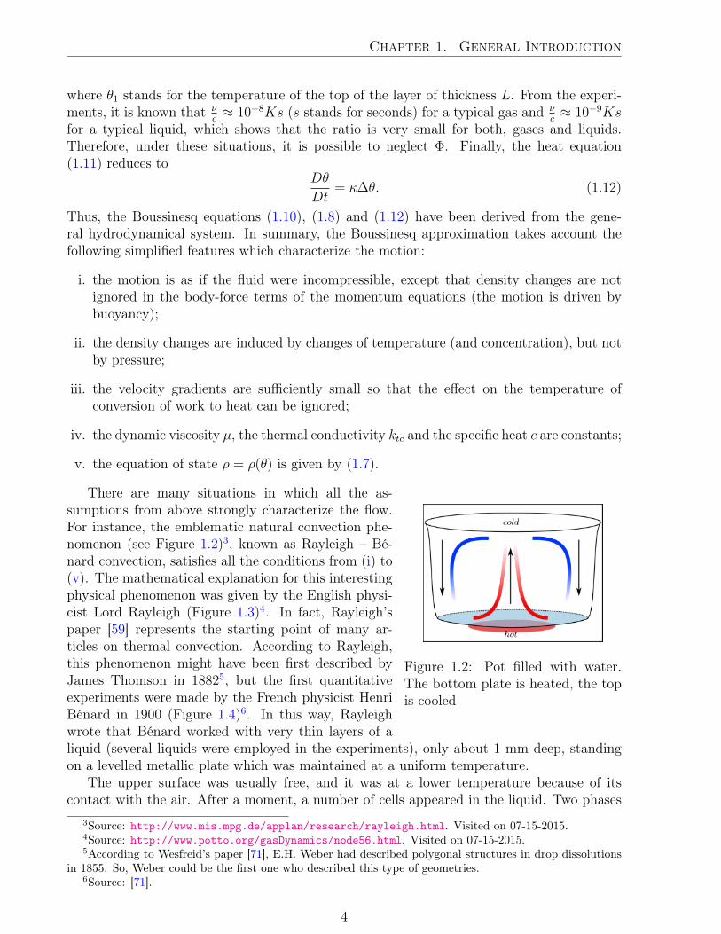
Figure 1.2: Pot filled with water.The bottom plate is heated, the topis cooled

There are many situations in which all the as-sumptions from above strongly characterize the flow.For instance, the emblematic natural convection phe-nomenon (see Figure 1.2)3, known as Rayleigh – Bé-nard convection, satisfies all the conditions from (i) to(v). The mathematical explanation for this interestingphysical phenomenon was given by the English physi-cist Lord Rayleigh (Figure 1.3)4. In fact, Rayleigh’spaper [59] represents the starting point of many ar-ticles on thermal convection. According to Rayleigh,this phenomenon might have been first described byJames Thomson in 18825, but the first quantitativeexperiments were made by the French physicist HenriBénard in 1900 (Figure 1.4)6. In this way, Rayleighwrote that Bénard worked with very thin layers of aliquid (several liquids were employed in the experiments), only about 1 mm deep, standingon a levelled metallic plate which was maintained at a uniform temperature.

The upper surface was usually free, and it was at a lower temperature because of itscontact with the air. After a moment, a number of cells appeared in the liquid. Two phases

3Source: http://www.mis.mpg.de/applan/research/rayleigh.html. Visited on 07-15-2015.4Source: http://www.potto.org/gasDynamics/node56.html. Visited on 07-15-2015.5According to Wesfreid’s paper [71], E.H. Weber had described polygonal structures in drop dissolutions

in 1855. So, Weber could be the first one who described this type of geometries.6Source: [71].

4

http://www.mis.mpg.de/applan/research/rayleigh.html

http://www.potto.org/gasDynamics/node56.html

1.1. Preliminaries

Figure 1.3: L. Rayleigh Figure 1.4: H. Bénard

are distinguished, of different duration, the first being relatively very short. The limit of thefirst phase is described as the “semi-regular cellular regime”; in this state all the cells havealready acquired surfaces nearly identical, their forms being nearly regular convex polygonsof, in general, 4 to 7 sides (see Figure 1.5)7.

Figure 1.5: Bénard cells underan air surface

The boundaries are vertical, and the circulation in eachcell occurs with an ascension of the liquid in the middle of acell and then the liquid descends at the common boundarybetween a cell and its neighbours. This phase is brief (1or 2 seconds) for the less viscous liquids such as alcohol,benzine, etc., at ordinary temperatures. But in the case ofvery viscous liquids such as oils, if the flux of heat is small,the deformations are extremely slow and the first phase maylast several minutes or more. The second phase has for itslimit a permanent regime of regular hexagons. During thisperiod the cells become equal, regular and align themselves.

Encouraged by Bénard’s experiments (see [71] to knowabout the scientific life of Henri Bénard), Rayleigh formu-lated the mathematical theory of convective instability ofa layer of fluid between horizontal planes by using of theBoussinesq equations (see [25], [74], [15]). Then, he showedthat instability would occur only when the temperature gra-dient was so large such that the dimensionless number gαβd4

κu

(nowadays called the Rayleigh number) exceeded a certaincritical value. Here g is the value of the acceleration due to gravity, α the coefficient of ther-mal expansion of the fluid, β the magnitude of the vertical temperature gradient of the basicstate of rest, d the depth of the layer of the fluid, κ its thermal diffusivity and ν its kinematicviscosity. Physically speaking, Rayleigh number measures the ratio of the destabilizing effectof buoyancy to the stabilizing effects of diffusion and dissipation.

It is worth to note that although Pearson [57] proved that most of the motions observed byBénard were driven by the variation of surface tension with temperature and not by thermalinstability of light fluid below heavy fluid, the convection in a horizontal layer of fluid heatedfrom below is still called Bénard convection. However, Rayleigh’s model is in accord withexperiments on layers of fluid with rigid boundaries and on thicker layers with a free surface,because the variation of surface tension diminishes as the thickness of the layer increases.

In conclusion, the assumption (1.7) for the density requires that the maximum value of

7Source: [25]

5


α(θ−θ0) is small compared to 1, that means, α(θ−θ0)∗ 1, where (θ−θ0)∗ is the maximumvalue of (θ − θ0), see [31]. When this is true, it can be demonstrated that density variationsdue to changing temperature are negligible in both the continuity (1.2) and heat flow (1.5)equations, but dominant in the equation of motion (1.3). It is important to mention that theBoussinesq approximation is more appropriate for shallow layers of liquid (as in laboratoryexperiments) where hydrostatic compression is not important. However, for deep layers orfor compressible fluids, equation (1.7) is not suitable. Thus, in addition to the requirementof small values of α(θ− θ0), the Boussinesq approximation is only valid when the depth d ofthe convecting layer is small compared to the scale height H over which significant densityvariations occur, see [64], [24, p. 6] and [37, p. 135]. Further, more typically, assumptions (iv)and (v) do not hold. For example, the condition (v) is not fulfilled when treating convectionnear the critical point (4C) at which the density of water has a relative maximum, see [33],because a nonlinear equation of state ρ = ρ(θ) arises. In very large scale systems (typicalin geo-astrophysical applications) the variations of material properties cannot be neglected,then the condition (iv) is not fulfilled. Moreover, for flows in which the Mach number issensibly different from zero (for example, in propagation of sound or shock waves), the factthat the velocity field is solenoidal and the independence of density on pressure are lost, andthen conditions (i) and (ii) are not suitable for this kind of problems. Also, the Boussinesqapproximation cannot be applied to high-speed gas flows where density variations inducedby velocity divergence cannot be neglected. It is interesting to note that the Boussinesqequations are obtained as an asymptotic limit of the complete Navier-Stokes equations, see[46] for details.

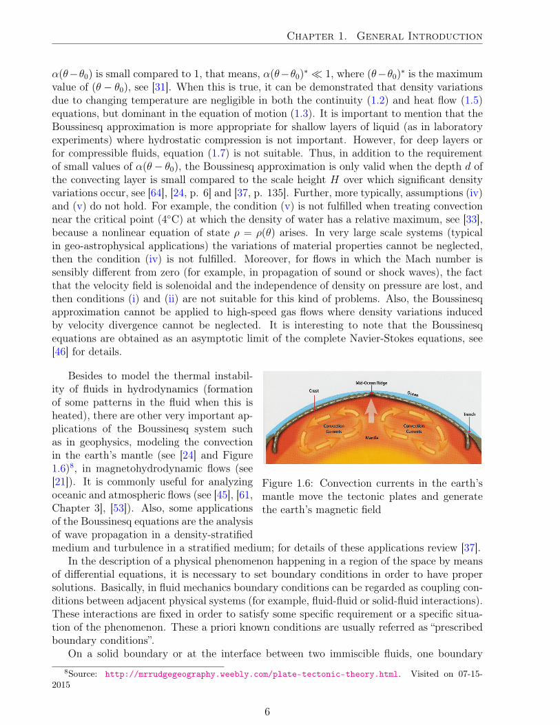
Figure 1.6: Convection currents in the earth’smantle move the tectonic plates and generatethe earth’s magnetic field

Besides to model the thermal instabil-ity of fluids in hydrodynamics (formationof some patterns in the fluid when this isheated), there are other very important ap-plications of the Boussinesq system suchas in geophysics, modeling the convectionin the earth’s mantle (see [24] and Figure1.6)8, in magnetohydrodynamic flows (see[21]). It is commonly useful for analyzingoceanic and atmospheric flows (see [45], [61,Chapter 3], [53]). Also, some applicationsof the Boussinesq equations are the analysisof wave propagation in a density-stratifiedmedium and turbulence in a stratified medium; for details of these applications review [37].

In the description of a physical phenomenon happening in a region of the space by meansof differential equations, it is necessary to set boundary conditions in order to have propersolutions. Basically, in fluid mechanics boundary conditions can be regarded as coupling con-ditions between adjacent physical systems (for example, fluid-fluid or solid-fluid interactions).These interactions are fixed in order to satisfy some specific requirement or a specific situa-tion of the phenomenon. These a priori known conditions are usually referred as “prescribedboundary conditions”.

On a solid boundary or at the interface between two immiscible fluids, one boundary8Source: http://mrrudgegeography.weebly.com/plate-tectonic-theory.html. Visited on 07-15-

2015

6

http://mrrudgegeography.weebly.com/plate-tectonic-theory.html

1.1. Preliminaries

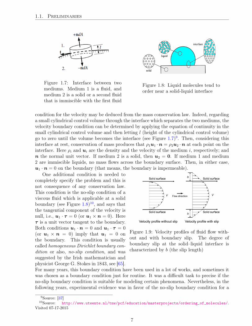
Figure 1.7: Interface between twomediums. Medium 1 is a fluid, andmedium 2 is a solid or a second fluidthat is immiscible with the first fluid

Figure 1.8: Liquid molecules tend toorder near a solid-liquid interface

condition for the velocity may be deduced from the mass conservation law. Indeed, regardinga small cylindrical control volume through the interface which separates the two mediums, thevelocity boundary condition can be determined by applying the equation of continuity in thesmall cylindrical control volume and then letting l (height of the cylindrical control volume)go to zero until the volume becomes the interface (see Figure 1.7)9. Then, considering thisinterface at rest, conservation of mass produces that ρ1u1 ·n = ρ2u2 ·n at each point on theinterface. Here ρi and ui are the density and the velocity of the medium i, respectively; andn the normal unit vector. If medium 2 is a solid, then u2 = 0. If medium 1 and medium2 are immiscible liquids, no mass flows across the boundary surface. Then, in either case,u1 · n = 0 on the boundary (that means, the boundary is impermeable).

Figure 1.9: Velocity profiles of fluid flow with-out and with boundary slip. The degree ofboundary slip at the solid–liquid interface ischaracterized by b (the slip length)

One additional condition is needed tocompletely specify the problem and this isnot consequence of any conservation law.This condition is the no-slip condition of aviscous fluid which is applicable at a solidboundary (see Figure 1.8)10, and says thatthe tangential component of the velocity isnull, i.e., u1 · τ = 0 (or u1 × n = 0). Hereτ is a unit vector tangent to the boundary.Both conditions u1 · n = 0 and u1 · τ = 0(or u1 × n = 0) imply that u1 = 0 onthe boundary. This condition is usuallycalled homogeneous Dirichlet boundary con-dition or also, no-slip condition, and wassuggested by the Irish mathematician andphysicist George G. Stokes in 1843, see [65].For many years, this boundary condition have been used in a lot of works, and sometimes itwas chosen as a boundary condition just for routine. It was a difficult task to precise if theno-slip boundary condition is suitable for modeling certain phenomena. Nevertheless, in thefollowing years, experimental evidence was in favor of the no-slip boundary condition for a

9Source: [37]10Source: http://www.utwente.nl/tnw/pcf/education/masterprojects/ordering_of_molecules/.

Visited 07-17-2015

7

http://www.utwente.nl/tnw/pcf/education/masterprojects/ordering_of_molecules/


large class of flows, and it became widely accepted for most liquid flows.Relatively recent, it was showed in a rigourously way why a viscous fluid cannot slip on a

wall covered by microscopic asperities (rugose wall), see [14], allowing the acceptance of theno-slip boundary condition. While this assumption has proved to be highly successful for agreat variety of flow conditions, it has been found to be inadequate in certain situations suchas in the mechanics of thin films, problems involving multiple interfaces, the flow of rarefiedfluids, the flow of a liquid in a domain which has air as part of its boundary, the flow of afluid in perforated domains, flow of blood through blood vessels (see [70]), the flow of a fluidregarding free boundary, etc. In this situation, the French engineering Claude Navier (see[51])11, in 1823, proposed that the tangential velocity should be proportional to the tangentialstress on the boundary, i.e., 2 [D(u)n]τ + α uτ = 0, where D(u) = 1

2

(∇u+ (∇u)T

)is the

deformation tensor (or linearized strain tensor) associated with the velocity field u and αis a friction function. The condition of impermeability of the boundary together with thislast condition is known as the Navier boundary condition (see Figure 1.9)12. When α isa positive function, this condition is called a slip boundary condition with linear friction.Lately, the Navier boundary condition has raised its interest to the scientific community dueto the interesting applications in modeling of physical phenomena such as in the examplesmentioned before.

1.2 Thesis Description and Main Results

The work carried out in this thesis covers the research done along three years under a jointsupervised doctoral thesis between the University of Chile and the Université de Pau et desPays de l’Adour.

This work will be focusing in the Lp-theory for the stationary Boussinesq system (1.1)regarding two different types of boundary conditions for the velocity field: in the first chapter,we consider the Dirichlet boundary condition

u = ub on Γ, (1.13)

where Γ denotes the boundary of the domain; meanwhile in the second one, the velocity fieldwill have attached the Navier boundary condition

u · n = 0, 2 [D(u)n]τ + α uτ = a, on Γ. (1.14)

Further, the boundary condition for the temperature will be, in both chapters, the Dirichletboundary condition

θ = θb on Γ. (1.15)

Next sections are dedicated to describe the main results of this work, leaving all the detailsfor the subsequent chapters.

11After almost half of a century, Maxwell [44] derived this condition from the kinetic theory of gases12Source: http://www.beilstein-journals.org/bjnano/single/articleFullText.htm?publicId=

2190-4286-2-9. Visited 07-17-2015

8

http://www.beilstein-journals.org/bjnano/single/articleFullText.htm?publicId=2190-4286-2-9

http://www.beilstein-journals.org/bjnano/single/articleFullText.htm?publicId=2190-4286-2-9

1.2. Thesis Description and Main Results

1.2.1 Boussinesq system with Dirichlet boundary conditions for thevelocity field

In chapter 2, the stationary Boussinesq system (1.1) is studied with the boundary con-ditions (1.13) and (1.15). The aim is to develop the Lp-theory for this problem, meaningwith Lp-theory, the study of the existence of generalized solutions in W 1,p, strong solutionsin W 2,p and very weak solutions in Lp.

This chapter has seven sections. In the first section we describe the problems underconsideration and related literature. The second section is dedicated to summarize the mainresults of this chapter. The third section will be focusing on standardizing the notationto be used along the chapter and it will be given some useful statements which will playan important role in the proof of the main results. The fourth section will deal with theexistence of weak solutions for (1.1)-(1.13)-(1.15) in the Hilbert case. This result, whoseproof is based on applying the Leray-Schauder fixed point theorem, is established as follows.

Let Ω ⊂ R3 be an open, bounded and connected set with Lipschitz boundary Γ and let

g ∈ L32 (Ω), h ∈ H−1(Ω), ub ∈H

12 (Γ), θb ∈ H

12 (Γ) (1.16)

such that∫

Γub · n ds = 0. There exists δ1 = δ1(Ω) > 0 such that if

1

ν

m∑i=1

∣∣∣∣∫Γi

ub · n ds

∣∣∣∣ ≤ δ1,

then problem (1.1)-(1.13)-(1.15) has at least one weak solution (u, π, θ) ∈H1(Ω)×L2(Ω)/R×H1(Ω). Further, if ub = 0 and θb = 0, then the weak solution (u, θ) satisfies the followingestimates:

‖∇u‖L2(Ω) ≤C

νκ‖g‖

L32 (Ω)‖h‖H−1(Ω),

‖∇θ‖L2(Ω) ≤C

κ‖h‖H−1(Ω),

with C = C(Ω) > 0.The fifth section is concerned with the Lp-regularity results for the Hilbertian weak

solution. They are proved by using the regularity of the Poisson and the Stokes equations,and a suitable bootstrap argument. In this way, let Ω ⊂ R3 be more regular than before (ofclass C1,1). It is supposed that

g ∈ Lr(Ω), h ∈ W−1,p(Ω) and (ub, θb) ∈W 1− 1p,p(Γ)×W 1− 1

p,p(Γ)

with p > 2, r = max

32, 3p

3+p

if p 6= 3 and r = 3

2+ ε if p = 3 for any fixed

0 < ε < 12. Then the weak solution in H1(Ω) for the Boussinesq system satisfies

(u, π, θ) ∈W 1,p(Ω)× Lp(Ω)/R ×W 1,p(Ω).

Moreover, if

g ∈ Lr(Ω), h ∈ Lp(Ω) and (ub, θb) ∈W 2− 1p,p(Γ)×W 2− 1

p,p(Γ)

with p ≥ 65, r = max

32, p

if p 6= 32

and r = 32

+ ε if p = 32for any fixed 0 < ε < 1

2.

Then the weak solution in H1(Ω) for the Boussinesq system satisfies

(u, π, θ) ∈W 2,p(Ω)×W 1,p(Ω)/R ×W 2,p(Ω).

9


It is observed that the choice of the space for g is optimal to study W 1,p(Ω)-regularity withp > 2 and W 2,p(Ω)-regularity with p ≥ 6

5.

The sixth section deals with the existence and uniqueness of the very weak solution forthe Boussinesq system (the definition is given in Section 2.6). So, if Ω ⊂ R3 is of class C1,1,and letting 3 ≤ p, r <∞,

ub ∈W− 1p,p(Γ) with < ub · n, 1 >Γ= 0, g ∈ Lq(Ω),

h ∈ W−1, prp+r (Ω), θb ∈ W− 1

r,r(Γ),

where q = maxs, 3

2+ εfor any fixed 0 < ε < 1

2and s given by

s > r′ if p = 3, and s =3rp

2rp+ 3(r − p)if p > 3 and

1

r≤ 1

p+

2

3,

where, in the case p > 3, s is chosen such that

1

r+

1

s+

1

(p′)∗∗= 1 with

1

(p′)∗∗=

1

p′− 2

3.

Then, there exists δ2 = δ2(Ω) > 0 such that if

1

ν

m∑i=1

∣∣〈ub · n, 1〉Γi∣∣ ≤ δ2,

then there exists at least one very weak solution (u, π, θ) ∈ Lp(Ω)×W−1,p(Ω)/R×Lr(Ω) of(1.1)-(1.13)-(1.15). Further, if g ∈ Lt(Ω), where t = max s, 2, and if(

1

ν+

1

κ

)(‖ub‖

W− 1p ,p(Γ)

+

(1

ν+

1

κ

)‖g‖Lt(Ω)

(1

κ‖h‖

W−1,

prp+r (Ω)

+ ‖θb‖W− 1r ,r(Γ)

))≤ δ3

for some δ3 = δ3(p, r, t,Ω) > 0, then this solution is unique.This last result tells that it is possible to show the existence of very weak solutions for the

Boussinesq system, if we just consider smallness of the fluxes of ub through each connectedcomponent Γi of the boundary Γ, as in the case of Navier-Stokes equations, see Amrouche -Rodríguez [6] or in the linear Stokes case, see Conca [19].

Unlike the result showed in Kim [35], two important facts are taken into account. Firsta more general type of domain regarding a possible disconnected boundary is consideredallowing in this way other kind of domains to analyze this system of equations. And second,the space where g lies is enlarged and hence the hypothesis L∞(Ω) can be weakened andresults for very weak solutions for the Boussinesq system can still be obtained.

Furthermore, it is possible to extend the regularity of the solution of (1.1)-(1.13)-(1.15)for 3

2≤ p < 2 in W 1,p(Ω) and for 1 < p < 6

5in W 2,p(Ω), by means of using some uniqueness

and regularity results for the Oseen problem. Finally, seventh section is devoted to showsomeH1(Ω)-estimates for the weak solution, and this serves as a tool to show the uniquenessof this solution.

10


1.2.2 Boussinesq system with Navier boundary conditions for thevelocity field

Chapter 3 is concerned with the study of the stationary Boussinesq system (1.1) with theboundary conditions (1.14) and (1.15). The idea is to study the existence of weak solutionsin the Hilbert caseH1(Ω), generalized solutions inW 1,p(Ω) and strong solutions inW 2,p(Ω).

Before starting the description of the structure of the next two chapters, we consider thefollowing hypothesis for the friction function α which will be used along the next sections:there exists a real number α∗ such that

α ≥ α∗ ≥ 0 withα∗ ≥ 0 if Ω is not axisymmetric, orα∗ > 0 (or even, α(x) > 0 a.e. x ∈ Γ) otherwise.

(H)

This chapter is composed by five sections. Similarly as in Chapter 1, first, second andthird sections are concerned with the introduction of the Boussinesq problem, a review ofsome literature related to this problem, the main results of this chapter, the standardizationof the notation to be used along this chapter and the presentation of some useful assertionswhich will play an important role in the proof of the main results. It is noteworthy that oneof this important assertions is a Korn-type inequality. This type of inequality is very usefulin problems where the deformation tensor appears. The fourth section is dedicated to theexistence of weak solutions for (1.1)-(1.14)-(1.15) in the Hilbert case. Indeed, let Ω ⊂ R3 bea bounded domain of class C2,1 and let

g ∈ L32 (Ω), h ∈ H−1(Ω), α ∈ L2+ε(Γ) satisfying (H) for any ε > 0 sufficiently small,

a ∈H−12 (Γ) such that a · n = 0 on Γ, θb ∈ H

12 (Γ).

Then, problem (1.1)-(1.14)-(1.15) has a weak solution (u, π, θ) ∈H1(Ω)×L2(Ω)/R×H1(Ω).Further, if θb = 0 on Γ, u and θ satisfy the following estimates:

‖u‖H1(Ω) ≤M1

ν

(ν‖a‖

H−12 (Γ)

+1

κ‖h‖H−1(Ω)‖g‖L 3

2 (Ω)

),

‖∇θ‖L2(Ω) ≤M1

κ‖h‖H−1(Ω),

with M1 = M1(Ω) > 0 independent of α. Moreover, if there exists γ = γ(Ω) > 0 such that

νκ ≥ γ‖g‖L

32 (Ω)‖θb‖H 1

2 (Γ),

then‖u‖H1(Ω) ≤

M2

ν

(ν‖a‖

H−12 (Γ)

+ ‖θ‖H1(Ω)‖g‖L 32 (Ω)

),

‖θ‖H1(Ω) ≤M2

[(1 +

1

κ‖a‖

H−12 (Γ)

)‖θb‖H 1

2 (Γ)+

1

κ‖h‖H−1(Ω)

],

with M2 = M2(Ω, γ) > 0 independent of α. The proof of this result is based on applying theLeray-Schauder fixed point theorem.

Finally, in the fifth section, a study of the W 1,p and W 2,p regularity of the weaksolutions for the problem (1.1)-(1.14)-(1.15) will be carried out. The proof is done by taking

11


advantage of the regularity results for the Poisson equation with Dirichlet boundary conditionand Stokes problem with Navier boundary condition. Indeed, supposing that

g ∈ Lr(Ω), h ∈ W−1,p(Ω), α ∈ Lt∗(p)(Γ) satisfying (H)

with t∗(p) defined by (4.14) and (a, θb) ∈W− 1p,p(Γ)×W 1− 1

p,p(Γ)

withp > 2, r = max

3

2,

3p

3 + p

if p 6= 3 and r =

3

2+ ε if p = 3

for any ε > 0 sufficiently small. Then the weak solution for (1.1)-(1.14)-(1.15) satisfies

(u, π, θ) ∈W 1,p(Ω)× Lp(Ω)/R ×W 1,p(Ω).

Moreover, if g ∈ Lr(Ω), h ∈ Lp(Ω),

α ∈ H12 (Γ) if

6

5≤ p ≤ 2; α ∈ H

12

+ε(Γ) if 2 0 sufficiently small. Then the solution for (1.1)-(1.14)-(1.15) satisfies

(u, π, θ) ∈W 2,p(Ω)×W 1,p(Ω)/R ×W 2,p(Ω).

1.2.3 Stokes equations with Navier boundary condition

In Chapter 4, we deal with the study of the stationary Stokes equations−∆u+∇π = f in Ω,div u = χ in Ω,u · n = g on Γ,2 [D(u)n]τ + α uτ = h on Γ,

where Ω ⊂ R3 is a bounded domain of class C1,1, Γ is the boundary of Ω, u and π arethe velocity and pressure of the fluid, respectively, D(u) = 1

2

(∇u+ (∇u)T

)is the strain

tensor associated with the velocity field u, n is the unit outward normal vector, τ is thecorresponding unit tangent vector, f is an external force acting on the fluid, χ and g standfor the compressibility and permeability conditions, respectively, α is a friction scalar functionand h is a tangential vector field on the boundary. In the case α > 0, the Navier boundarycondition is said to be a boundary condition with linear friction. In this chapter α will satisfy(H).

We are interested in the study of the existence of a unique weak solutionH1(Ω), a uniquegeneralized solution in W 1,p(Ω) and a unique strong solution in W 2,p(Ω).

In order to attain these results, we organize the chapter as follows: in the first sectionwe introduce the problem to be considered. Second section provides a summary of the

12


main results of this chapter. The notation to be used along this chapter and the presentationof some useful results will be treated in the third section. The fourth section is dedicatedto prove the existence of a unique weak solution for the Stokes problem in H1(Ω). Indeed,let Ω be a bounded domain of class C1,1 and let us suppose χ = 0 and g = 0. Also, let

f ∈ L65 (Ω), h ∈H−

12 (Γ) such that h · n = 0 on Γ, α ∈ L2(Γ)

with α verifying the hypothesis (H). Then the Stokes problem has a unique solution (u, π) ∈H1(Ω)× L2(Ω)/R which satisfies the estimate

‖u‖H1(Ω) + ‖π‖L2(Ω)/R ≤ C(Ω, α∗)(‖f‖

L65 (Ω)

+ ‖h‖H−

12 (Γ)

)where

C(Ω, α∗) =

C(Ω) under the hypothesis (H1)C(Ω)

min1,α∗ under the hypothesis (H2) with α ≥ α∗ > 0

C(Ω) under the hypothesis (H2) with α(x) > 0 a.e. x ∈ Γ.

We use the very useful Lax-Milgram theorem to prove the previous assertion.Finally, in the fifth section, a study of the W 1,p(Ω) for p > 2 and W 2,p(Ω) for p ≥ 6

5is

carried out. In support of this, let us suppose χ = 0, g = 0,

f ∈ Lr(p)(Ω) with r(p) is defined by (4.1), h ∈W− 1p,p(Γ) such that h · n = 0 on Γ,

and α ∈ Lt∗(p)(Γ) satisfying (H) with

t∗(p) =

2 + ε if 2 3,

where ε > 0 is an arbitrary number sufficiently small. Then the Stokes problem has a uniquesolution (u, π) ∈W 1,p(Ω)× Lp(Ω)/R. Furthermore, let us suppose

f ∈ Lp(Ω), h ∈W 1− 1p,p(Γ) such that h · n = 0 on Γ,

and

α ∈ H12 (Γ) if

6

5≤ p ≤ 2; α ∈ H

12

+ε(Γ) if 2 0 is an arbitrary number sufficiently small and α satisfies (H). Then the weaksolution for the Stokes problem satisfies that (u, π) ∈W 2,p(Ω)×W 1,p(Ω)/R.

The key of the proof of this result is to take advantage of the regularity results for theStokes problem with Navier boundary condition when α = 0.

13

Chapter 2

Boussinesq system with Dirichletboundary conditions

AbstractIn this chapter we consider the stationary Boussinesq system with non-homogeneous

Dirichlet boundary conditions in a bounded domain Ω ⊂ R3 of class C1,1 with a possiblydisconnected boundary. Assuming that the fluxes of the velocity across each connectedcomponent of the boundary are sufficiently small, we prove the existence of weak, strong andvery weak solutions of the stationary Boussinesq system in Lp-theory. As it is expected, weobtain the uniqueness of the solution by considering small data.

Keywords: Boussinesq system, natural convection, non-homogeneous Dirichlet boundaryconditions, existence, uniqueness, Lp-regularity, weak solution, strong solution, very weaksolution

2.1 IntroductionThe work developed in this chapter is concerned with the existence, uniqueness and regu-larity of the solution for the stationary Boussinesq system with Dirichlet non-homogeneousboundary conditions. Let Ω ⊂ R3 be a bounded domain of class C1,1. Consider the stationaryBoussinesq system as follows:

−ν∆u+ (u · ∇)u+∇π = θg in Ω,div u = 0 in Ω,

−κ∆θ + u · ∇θ = h in Ω,u = ub , θ = θb on Γ,

(BS )

where Γ is the boundary of Ω which is not necessarily connected, i.e., it could be the disjointunion of its connected components Γi, with i = 0, 1, . . . ,m. In this context, Γ0 will representthe exterior boundary which contains Ω and all the boundaries Γj, j = 1, . . . ,m. Theunknowns are u, π and θ which represent the velocity field, the pressure and the temperatureof the fluid, respectively. The data are ν > 0 the kinematic viscosity of the fluid, κ > 0 thethermal diffusivity of the fluid, g the gravitational acceleration, h a heat source applied onthe fluid, ub the velocity at the boundary and θb the temperature at the boundary. As wecan see, this system of partial differential equations is formed by coupling the stationaryNavier-Stokes equations and the stationary convection-diffusion equation for heat transfer.

14

2.1. Introduction

Keep in mind the following facts concerning g. Along this chapter, we will considera non-zero gravitational acceleration g. This assumption is not a strong or an unusualconstraint over g, on the contrary, in all the physical phenomena which are carried out intoa gravitational field (like the Earth’s gravitational field), gravity plays an important role inthe development of such phenomena. In particular, in the Boussinesq approximation, thegravitational acceleration is the keystone of this formulation. Mathematically, if we considerg = 0, then the Navier-Stokes equations and the convection-diffusion equation are decoupled,hence we loose the essential aspect of the Boussinesq system and we end by analyzing adifferent physical problem. Further, it is noteworthy that in practical cases, the gravitationalacceleration g, in fact, belongs to L∞(Ω), but we consider important to relax this assumptionfor mathematical purposes. This means we can enlarge the space where g lies and we canstill get solutions for our problem.

The Boussinesq system is considered as a good approximation to model the natural (orfree) convection phenomenon. This physical phenomenon is a way of heat transfer which iscarried out by the motion of the fluid without using external devices to produce that motion(forced convection), but only by the density differences resulting from temperature gradientswithin the fluid. We have an emblematic example of this phenomenon when we heat a potof water. Indeed, when we start heating the pot, the water at the bottom of the pot beginsto be heated firstly. This produces a reduction in the density of this part of the water andconsequently, it rises to the surface. On the other hand, the water at the top of the pot iscolder than the one at the bottom, consequently, its density is higher and hence, it descendsto the bottom of the pot. This process is repeated again and again, generating circularcurrents in the water, known as convection currents, causing all the water moves inside thepot and with this, the water is completely heated.

The Boussinesq approximation was proposed by the French mathematician and physi-cist Joseph Boussinesq at the beginning of the twentieth century (1903) on his monograph[13]. From that time until our days, there have been many works related with this system,showing us the importance that it has had in theoretical and applied mathematics, physics,oceanography and many other sciences. Apart from Joseph Boussinesq’s monograph, we havesome references which address the mathematical deduction of the Boussinesq system, see, forexample, [15, 10]. Also, there is an interesting work concerning the life of Joseph Boussinesq,the idea that led him to deduce this system and the applicability of his approximation invarious physical problems, see [73].

What do we know about the solvability of the Boussinesq system when our domain has anon-connected boundary? Let us see some details. From the continuity equation we obtainthe following necessary compatibility condition for the boundary data ub, in order to solvethe Boussinesq system: ∫

Γ

ub · n ds =m∑i=0

∫Γi

ub · n ds = 0, (2.1)

where n denotes the outward unit normal vector to Γ. It is important to mention that theexistence of solutions for the Navier-Stokes equations and, consequently, for the Boussinesqsystem, considering merely the condition (2.1), is an open problem yet. In fact, during along time the existence of weak solutions for the Navier-Stokes equations was proven underthe following condition: ∫

Γi

ub · n ds = 0 for all i = 0, . . . ,m, (2.2)

15

Chapter 2. Boussinesq system with Dirichlet boundary conditions

see, for example, [40, 39, 20]. Clearly, condition (2.2) is stronger than (2.1) and, further,(2.2) does not allow the presence of sinks and sources along the boundary.

Afterwards, it was possible to prove existence of weak solutions for the Navier-Stokesequations weakening the condition (2.2) by assuming only smallness of these fluxes, see[12, 36, 27]. However, there are some special cases where the existence of weak solutionsfor the Navier-Stokes equations is known just considering the condition (2.1) without anyinformation about the size of the fluxes across each connected component of the boundary.These special cases consider some symmetry hypothesis on the domain Ω ⊂ Rd, d = 2 or 3,and on the velocity boundary data ub, see [3, 49, 58, 26].

In connection with the stationary Boussinesq system, Morimoto [50] recently proved theexistence of weak solutions considering the condition (2.2) and also proved the existence ofweak solutions in the case of a symmetric planar domain and symmetric boundary data ubconsidering just the condition (2.1).

There are other related works concerning the stationary Boussinesq system as for examplesome contributions done by Morimoto. Morimoto [47] studied the existence of weak solutionsand their interior regularity (C∞ regularity), in the case of a bounded domain Ω in R3

with C2 connected boundary Γ which is divided in two disjoint subsets Γ1 and Γ2. Theboundary conditions considered were Dirichlet homogeneous on the velocity and mixed onthe temperature (Dirichlet non-homogeneous condition on Γ1 and Neumann homogeneouscondition on Γ2). In a next work, assuming now that Ω is a bounded domain in Rd, d ≥ 2,with C1 connected boundary Γ whose structure is the same as it was considered in [47],Morimoto extended his previous result on existence of weak solutions considering, this time,Neumann non-homogeneous condition on Γ2. This time, he gave a result of uniquenessby imposing smallness condition on the norm of the solution, see [48]. In both articles,Morimoto took the gravitational acceleration g in L∞(Ω) and did not consider a heat sourcein the convection-diffusion equation.

Assuming that Ω is a bounded domain in Rd, d = 2 or 3, with Lipschitz connectedboundary Γ, and considering the same structure of the boundary as in the articles of Morimoto[47, 48], Bernardi, Métivet and Pernaud-Thomas [10] proved existence and uniqueness of theweak solution for the Boussinesq system, considering Dirichlet non-homogeneous boundarycondition for the velocity field, extending, in this manner, the results given by Morimoto.They considered, on the right hand side of the Navier-Stokes equations, a function whichdepends on the temperature and is continuously differentiable with bounded derivative and,also, they included a heat source in the convection-diffusion equation. It is interesting to notethat for proving the existence of weak solutions, they used an important tool from nonlinearanalysis: the topological degree theory. As in the work [48], they showed uniqueness if thenorm of the solution is sufficiently small.

Let us see that there are other works about weak solutions for the stationary Boussinesqsystem which address other types of interesting problems. For instance, Gil’ [28] studied theexistence of weak solutions for a stationary Boussinesq system which appears in heat-masstransfer theory, in which, apart from consider the velocity and the temperature of the fluid,it takes account the concentration of material in a liquid. Kuraev [38] studied the existenceof weak solutions considering a nonlinear boundary condition for the temperature in one partof the boundary. Also, we can find some works concerning the study of weak solutions forthis system in exterior domains, see, for example, [56, 52].

As in the case of Stokes equations and Navier-Stokes equations, see [19, 6], concerningthe work with very weak solutions for the Boussinesq system we refer two articles. Santos da

16

2.2. Main results

Rocha, Rojas-Medar M. A. and Rojas-Medar M. D. [60] studied the existence and uniquenessof the very weak solution (u, π, θ) ∈ L3(Ω)×W−1,3(Ω)×L2(Ω) for the stationary Boussinesqsystem with Dirichlet non-homogeneous boundary conditions in L2(Γ) in a bounded domainof R3 with smooth enough connected boundary. Further, they considered the gravitationalacceleration g ∈ L3(Ω) and did not consider a heat source in the convection-diffusion equa-tion. The proof of the existence was based on the Leray-Schauder fixed point theorem andthe uniqueness was showed for sufficiently large viscosity. Recently, Kim [35] studied theexistence and uniqueness of the very weak solution (u, π, θ) ∈ Lq(Ω)×W−1,q(Ω)× Lr(Ω) ofthe stationary Boussinesq system with Dirichlet non-homogeneous boundary conditions inW− 1

q,q(Γ)×W− 1

r,r(Γ) in a bounded domain Ω ⊂ Rd, d = 2 or 3, with connected boundary Γ

of class C2. He considered the gravitational acceleration g ∈ L∞(Ω) and did not consider aheat source in the convection-diffusion equation. This article is taken as a base for this work.

In our work we are focused in showing existence, uniqueness and Lp regularity of the weaksolution for the stationary Boussinesq system with Dirichlet non-homogeneous boundaryconditions in a bounded domain Ω ⊂ R3 with boundary Γ of class C1,1 which is not necessarilyconnected, and also, we consider the gravitational acceleration g in a weaker space thanL∞(Ω) and the presence of a heat source in the convection-diffusion equation. We proveexistence of weak solutions in H1(Ω) just considering smallness of the fluxes of ub acrosseach connected component Γi of the boundary Γ by applying a Leray-Schauder fixed pointargument, and to prove uniqueness, we consider smallness condition on the norm of the data.In order to prove the regularity of the weak solution in W 1,p(Ω) with p > 2, and W 2,p(Ω)with p ≥ 6

5, we use the regularity results for the Stokes and Poisson equations combining

them with a bootstrap argument. For the regularity in W 1,p(Ω) and W 2,p(Ω) with 32≤ p < 2

and 1 < p < 65, respectively, first we need to study the existence of very weak solutions for

this system. With this result and using the existence and uniqueness of solutions for theOseen problem, we can establish the desired regularity of the solution.

The work is organized as follows: in section 2, we describe the main results of this work.Section 3 is devoted to introduce some notations and to precise some useful results. Insection 4, we study the existence of weak solutions of the stationary Boussinesq system. Theregularity of the weak solution in W 1,p(Ω) for p > 2 and in W 2,p(Ω) for p ≥ 6

5is dealt in

section 5. Later, in section 6 we deal with the study of very weak solutions and then, we canprove the regularity of the solution in W 1,p(Ω) for 3

2≤ p < 2 and in W 2,p(Ω) for 1 < p < 6

5.

Finally, thanks to the study done in section 6, we can derive estimates for the weak solutionin H1(Ω) and consequently, we obtain the uniqueness of such solution. This is derived insection 7.

2.2 Main resultsIn this section, we summarize the main results of this chapter. The first theorem is concernedwith the existence of weak solutions for the Boussinesq system. As you will realize, we justconsider smallness of the fluxes of ub across each connected component Γi of the boundaryΓ to obtain the existence.

Theorem 2.2.1 (weak solutions of the Boussinesq system in H1(Ω)). Let Ω ⊂ R3 be abounded domain with Lipschitz boundary Γ and let

g ∈ L32 (Ω), h ∈ H−1(Ω), ub ∈H

12 (Γ), θb ∈ H

12 (Γ)

17


such that∫


1

ν

m∑i=1

∣∣∣∣∫Γi

ub · n ds

∣∣∣∣ ≤ δ1,

then the problem (BS) has at least one weak solution (u, π, θ) ∈ H1(Ω) × L2(Ω) × H1(Ω).Further, if ub = 0 and θb = 0, then the weak solution (u, θ) satisfies the following estimates:

‖∇u‖L2(Ω) ≤C

νκ‖g‖

L32 (Ω)‖h‖H−1(Ω),

‖∇θ‖L2(Ω) ≤C

κ‖h‖H−1(Ω),

with C = C(Ω) > 0.

After the study of weak solutions in the case of Hilbert spaces, we are interested in studygeneralized and strong solutions in Lp-theory. In fact, the next two theorems deal with the Lpregularity of the weak solution of the Boussinesq system. In order to get these results, we usea classical bootstrap argument using regularity results of the Poisson and Stokes equations.Notice that for regularity in W 1,p(Ω), we begin by considering p > 2, and for regularity inW 2,p(Ω), we begin by considering p ≥ 6

5. For the cases 3

2≤ p < 2 in W 1,p(Ω) and 1 2). Let

h ∈ W−1,p(Ω) and (ub, θb) ∈W 1− 1p,p(Γ)×W 1− 1

p,p(Γ).

Let us suppose that

g ∈ Lr(Ω) with r = max

3

2,

3p

3 + p

if p 6= 3, and r =

3

2+ ε if p = 3

for any fixed 0 < ε < 12. Then the weak solution for the Boussinesq system given by Theorem

2.2.1 satisfies(u, π, θ) ∈W 1,p(Ω)× Lp(Ω)×W 1,p(Ω).

Theorem 2.2.3 (strong solutions in W 2,p(Ω) with p ≥ 65). Let

h ∈ Lp(Ω) and (ub, θb) ∈W 2− 1p,p(Γ)×W 2− 1

p,p(Γ).

Let us suppose that

g ∈ Lr(Ω) with r = max

3

2, p

if p 6= 3

2, and r =

3

2+ ε if p =

3

2

for any fixed 0 < ε < 12. Then the solution for the Boussinesq system given by Theorem 2.2.1

satisfies(u, π, θ) ∈W 2,p(Ω)×W 1,p(Ω)×W 2,p(Ω).

18

2.2. Main results

The next theorem is concerned with very weak solutions of the Boussinesq system. As inthe case of weak solutions, in order to show existence of very weak solutions, we just considersmallness of the fluxes of ub through each connected component Γi of the boundary Γ. Forproving uniqueness, we impose smallness condition on the norm of the data.

Theorem 2.2.4 (very weak solutions of the Boussinesq system). Let 3 ≤ p, r <∞,


h ∈ W−1, prp+r (Ω), θb ∈ W− 1

r,r(Γ),

where q = maxs, 3


2and s given by



1

r≤ 1

p+

2

3.

There exists δ2 = δ2(Ω) > 0 such that if

1

ν

m∑i=1

∣∣〈ub · n, 1〉Γi∣∣ ≤ δ2, (2.3)

then there exists at least one very weak solution (u, π, θ) ∈ Lp(Ω) ×W−1,p(Ω) × Lr(Ω) of(BS). Further, if g ∈ Lt(Ω), where t = max s, 2, and if(

1

ν+

1

κ

)(‖ub‖

W− 1p ,p(Γ)

+

(1

ν+

1

κ

)‖g‖Lt(Ω)

(1

κ‖h‖

W−1,

prp+r (Ω)

+ ‖θb‖W− 1r ,r(Γ)

))≤ δ3

for some δ3 = δ3(p, r, t,Ω) > 0, then this solution is unique.

The following two theorems deal with the regularity of the solution of the Boussinesqsystem in W 1,p(Ω) with 3

2≤ p < 2 and in W 2,p(Ω) with 1 < p < 6

5.

Theorem 2.2.5 (regularity W 1,p(Ω) with 32≤ p < 2). Let us suppose that

ub ∈W 1− 1p,p(Γ) satisfies (2.3), θb ∈ W 1− 1

p,p(Γ), h ∈ W−1,p(Ω) and g ∈ L

32

+ε(Ω)

for any fixed 0 < ε < 12. Then the very weak solution for the Boussinesq system given by

Theorem 2.2.4 satisfies

(u, π, θ) ∈W 1,p(Ω)× Lp(Ω)×W 1,p(Ω).

Theorem 2.2.6 (regularity W 2,p(Ω) with 1 < p < 65). Let us suppose that


p,p(Γ), h ∈ Lp(Ω) and g ∈ L

32

+ε(Ω)

for any fixed 0 < ε < 12. Then the very weak solution for the Boussinesq system given by

Theorem 2.2.4 satisfies

(u, π, θ) ∈W 2,p(Ω)×W 1,p(Ω)×W 2,p(Ω).

19


Finally, the next result shows the estimates for the weak solution in H1(Ω) and theuniqueness of such solution.

Theorem 2.2.7 (H1-estimates for the weak solution and uniqueness). Let

g ∈ L32 (Ω), h ∈ H−1(Ω), ub ∈H

12 (Γ), θb ∈ H

12 (Γ)

such that∫

Γub · n ds = 0. There exists δ4 = δ4(Ω) > 0 such that if(1

ν+

1

κ

)(‖ub‖H 1

2 (Γ)+

1

ν‖g‖

L32 (Ω)

(1

κ‖h‖H−1(Ω) + ‖θb‖H 1

2 (Γ)

))≤ δ4,

then the weak solution (u, π, θ) ∈ H1(Ω) × L2(Ω) × H1(Ω) of (BS) satisfies the followingestimates:

‖u‖H1(Ω) ≤ C

(‖ub‖H 1

2 (Γ)+

1

ν‖g‖

L32 (Ω)

(1

κ‖h‖H−1(Ω) + ‖θb‖H 1

2 (Γ)

)),

‖θ‖H1(Ω) ≤ C

(1

κ‖h‖H−1(Ω) + ‖θb‖H 1

2 (Γ)

),

with C = C(Ω) > 0. Moreover, if the data satisfy that(1

ν+

1

κ

)(‖ub‖H 1

2 (Γ)+

(1

ν+

1

κ

)‖g‖

L32 (Ω)

(1

κ‖h‖H−1(Ω) + ‖θb‖H 1

2 (Γ)

))≤ δ5

for some δ5 = δ5(Ω) > 0 such that δ5 ≤ δ4, then the weak solution of (BS) is unique.

2.3 Notations and some useful resultsThroughout this work, we consider Ω ⊂ R3 a bounded domain with boundary Γ of class C1,1.The term domain will be reserved for a nonempty open and connected set. In the case thatΩ be another kind of set, we will point it out. Bold font for spaces means vector (or matrix)valued spaces, and their elements will be denoted with bold font also. We will denote by nthe unit outward normal vector to Γ. Unless otherwise stated or unless the context otherwiserequires, we will write with the same positive constant all the constants which depend on thesame arguments in the estimations that will appear along this work.

We will denote as D(Ω) the set of smooth functions with compact support in Ω. Let usdefine the following spaces:

Dσ(Ω) = u ∈ D(Ω); div u = 0 in Ω,

H10,σ(Ω) = u ∈H1

0 (Ω); div u = 0 in Ω.Recall that Dσ(Ω) is dense in H1

0,σ(Ω), see [66, Theorem 1.6, p. 18]. Depending on thecontext, we use the following notation for the dual pairing:

〈f, ϕ〉Ω := 〈f, ϕ〉H−1(Ω),H10 (Ω) or 〈f, ϕ〉Ω := 〈f, ϕ〉

W−1,p(Ω),W 1,p′0 (Ω)

.

Observe that this notation depends on which spaces the functions belong and keep in mindthat it is also valid for vector valued functions.

Throughout this work, we use the following Sobolev inequality, see [39, Lemma 3, p. 10],and Poincaré inequality, which are valid for scalar and vector valued functions.

20

2.3. Notations and some useful results

Lemma 2.3.1. (i) Let Ω ⊂ R3 be a domain. There exists a positive constant A1, independentof Ω, such that for all ϕ ∈ H1

0 (Ω)

‖ϕ‖L6(Ω) ≤ A1‖∇ϕ‖L2(Ω).

(ii) Let Ω ⊂ R3 be a domain which is bounded at least in one direction. There exists a positiveconstant A2, depending on Ω, such that for all ϕ ∈ H1

0 (Ω)

‖ϕ‖H1(Ω) ≤ A2‖∇ϕ‖L2(Ω).

Let B and b be the following trilinear forms:

B (u,v,w) =

∫Ω

(u · ∇)v ·w dx for all (u,v,w) ∈(H1(Ω)

)3,

b (u, θ, τ) =

∫Ω

(u · ∇θ)τ dx for all u ∈H1(Ω), (θ, τ) ∈(H1(Ω)

)2.

Note, by using Hölder inequality, that

|B (u,v,w)| ≤ ‖u‖L6(Ω)‖∇v‖L2(Ω)‖w‖L3(Ω) (2.4)

and|b (u, θ, τ)| ≤ ‖u‖L6(Ω)‖∇θ‖L2(Ω)‖τ‖L3(Ω). (2.5)

The following lemmas deal with some of the main properties of the trilinear forms B and b.Both lemmas are easily proven by applying (2.4), (2.5) and Sobolev embedding theorem toshow the first claim and integration by parts to show the rest.

Lemma 2.3.2. Let Ω ⊂ R3 be an open set with Lipschitz boundary.(i) The trilinear form B is continuous in (H1(Ω))

3.(ii) B (u,v,w) = −B (u,w,v) for all (u,v,w) ∈ (H1(Ω))

3 with div u = 0 in Ω, andu · n = 0 or v = 0 or w = 0 on Γ.(iii) B (u,v,v) = 0 for all (u,v) ∈ (H1(Ω))

2 with div u = 0 in Ω, and u · n = 0 or v = 0on Γ.

Lemma 2.3.3. Let Ω ⊂ R3 be an open set with Lipschitz boundary.(i) The trilinear form b is continuous in H1(Ω)× (H1(Ω))

2.(ii) b (u, θ, τ) = −b (u, τ, θ) for all (u, θ, τ) ∈ H1(Ω) × (H1(Ω))

2 with div u = 0 in Ω, andu · n = 0 or θ = 0 or τ = 0 on Γ.(iii) b (u, θ, θ) = 0 for all (u, θ) ∈ H1(Ω) × H1(Ω) with div u = 0 in Ω, and u · n = 0 orθ = 0 on Γ.

When we address problems which involve Dirichlet non-homogeneous boundary conditionsand we want to study the existence of weak solutions for such kind of problems, we usually uselift functions for these boundary conditions. In our case, we are interested in the existence ofsuitable lift functions for the Dirichlet non-homogeneous boundary conditions on the velocityfield and the temperature.

The next lemma deals with the existence of a specific lift function for the boundarycondition on the velocity, which satisfies a convenient estimate. The complete proof of thislemma is given in [27, Lemma IX.4.2, p. 610].

21


Lemma 2.3.4. Let Ω ⊂ R3 be a bounded domain with Lipschitz boundary Γ and let ub ∈H

12 (Γ) such that ∫

Γ

ub · n ds = 0.

Then, for all ε > 0 there exists uεb ∈H1(Ω) such that

div uεb = 0, in Ω; uεb = ub, on Γ

and satisfies

|B (w,uεb,w)| ≤

ε+

m∑i=0

Ki

∣∣∣∣∫Γi

ub · n ds

∣∣∣∣‖∇w‖2

L2(Ω) (2.6)

for all w ∈H10,σ(Ω), where each Ki = Ki(Ω) > 0.

The following lemma is about the existence of a lift function for the boundary conditionon the temperature that satisfies a suitable estimate.

Lemma 2.3.5. Let Ω ⊂ R3 be a bounded open set with Lipschitz boundary Γ and let θb ∈H

12 (Γ). Then, for all η > 0 there exists θηb ∈ H1(Ω) such that θηb = θb on Γ and satisfies

‖θηb‖L3(Ω) ≤ η‖θb‖H 12 (Γ)

. (2.7)

Proof. To proof this lemma, we will use the idea given in [10, Lemma 2.8], but we introduceslight changes on it. Let us see some details. Since θb ∈ H

12 (Γ), we know that there exists

θ ∈ H1(Ω) such that θ = θb on Γ and

‖θ‖H1(Ω) ≤ C1‖θb‖H 12 (Γ)

with C1 = C1(Ω) > 0. Also, as Ω is bounded with Lipschitz boundary Γ, then the distancefunction d from x ∈ Ω up to the boundary Γ (d(x) = dist(x,Γ)) belongs to W 1,∞(Ω). Letε > 0 be an arbitrary number. We can define the function χε : Ω −→ [0, 1] as

χε(x) =

1 if 0 ≤ d(x) ≤ γ(ε)

2,

2(

1− 1γ(ε)

d(x))

if γ(ε)2≤ d(x) ≤ γ(ε),

0 if d(x) ≥ γ(ε),

where γ(ε) := exp(−1ε). Clearly, χε ∈ W 1,∞(Ω). Defining θεb = χεθ, we have that

‖θεb‖L3(Ω) ≤ C2 |Ωε1|

16 ‖θb‖H 1

2 (Γ),

where C2 = C2(Ω) > 0 and Ωε1 =

x ∈ Ω; 0 ≤ d(x) ≤ γ(ε)

. Since Ωε

1 is an annular region,it follows that

|Ωε1| ≤ C3γ(ε)

with C3 = C3(Ω) > 0. Further, due to the definition of γ(ε), it is possible to deduce that forall t > 0

|Ωε1|t ≤ C4ε

22


with C4 = C4(t,Ω) > 0. In particular, |Ωε1|

16 ≤ C4ε. Then

‖θεb‖L3(Ω) ≤ C5ε‖θb‖H 12 (Γ)

with C5 = C5(Ω) > 0. Finally, for any η > 0, we can choose ε = ηC5

and the estimate (2.7) isverified.

In part of our work, specifically, when we study the existence of very weak solutions for theBoussinesq system, we will use the following results concerning the existence and uniquenessof very weak solutions to the Poisson and Stokes equations.

First, let us consider the following Poisson problem:−κ∆θ = f in Ω,

θ = θb on Γ. (P)

Proposition 2.3.6. Let Ω ⊂ R3 be an open, bounded set of class C1,1. Let f ∈ W−1,t(Ω) andθb ∈ W− 1

r,r(Γ) with t = 1 + ε, for any fixed 0 < ε < 1 if 1 < r ≤ 3

2, and t = 3r

r+3if r > 3

2.

Then, the Poisson equation (P) has a unique very weak solution θ ∈ Lr(Ω), which satisfiesthe estimate

‖θ‖Lr(Ω) ≤ C

(1

κ‖f‖W−1,t(Ω) + ‖θb‖W− 1

r ,r(Γ)

),

where C > 0 is a constant depending only on ε, r and Ω when 1 < r ≤ 32, and depending

only on r and Ω when r > 32.

Proof. Since the Poisson equation is linear, it is possible to split the problem in two parts:−κ∆θ1 = f in Ω,

θ1 = 0 on Γ, (P1)−κ∆θ2 = 0 in Ω,

θ2 = θb on Γ. (P2)

Let us note that θ = θ1 + θ2 is the unique very weak solution for (P). Then, let us focusin the solutions of (P1) and (P2).

First of all, thanks to [6, Theorem 7], (P2) has a unique solution θ2 ∈ Lr(Ω) for all1 < r <∞, which satisfies

‖θ2‖Lr(Ω) ≤ C2‖θb‖W− 1r ,r(Γ)

with C2 = C2(r,Ω) > 0. Now, let us solve the problem (P1).

Case 1 < r ≤ 32

: Since f ∈ W−1,1+ε(Ω), by classical results of generalized solutions to thePoisson equation, we have that (P1) has a unique solution θ1 ∈ W 1,1+ε

0 (Ω) → L32

+ε′(Ω) forε′ = ε′(ε) > 0. Since 1 < r ≤ 3

2, then θ1 ∈ Lr(Ω), and satisfies

‖θ1‖Lr(Ω) ≤C1

κ‖f‖W−1,1+ε(Ω)

with C1 = C1(ε, r,Ω) > 0.

Case r > 32

: Since f ∈ W−1, 3rr+3 (Ω), by classical results of generalized solutions to the

Poisson equation, we have that (P1) has a unique solution θ1 ∈ W1, 3rr+3

0 (Ω) → Lr(Ω), andsatisfies

‖θ1‖Lr(Ω) ≤C1

κ‖f‖

W−1, 3r

r+3 (Ω)

with C1 = C1(r,Ω) > 0. Finally, taking C = maxC1, C2, we have the desired estimate.

23


Let us consider the following Stokes problem:−ν∆u+∇π = f in Ω,

div u = 0 in Ω,u = ub on Γ,

(S )

and let us introduce the following space:

Xr,p(Ω) =ϕ ∈W 1,r

0 (Ω); div ϕ ∈ W 1,p0 (Ω)

, 1 < r, p <∞,

whose dual space can be characterized as follows:

f ∈ (Xr,p(Ω))′ if and only if there exist F0 = (fij)1≤i,j≤3 such that F0 ∈ Lr′(Ω), f1 ∈

W−1,p′(Ω) and these satisfy that

f = ∇ · F0 +∇f1.

Moreover,‖f‖(Xr′,p′ (Ω))′ = max

‖fij‖Lr′ (Ω), 1 ≤ i, j ≤ 3 ; ‖f1‖W−1,p′ (Ω)

.

This characterization is proven in [6, Lemma 9]. Then, the following proposition is concernedwith the existence and uniqueness of the very weak solution of problem (S), see [6, Theorem11], for details of the proof.

Proposition 2.3.7. For any f ∈ (Xr′,p′(Ω))′ and ub ∈W− 1p,p(Γ) which satisfies

< ub · n,1 >W− 1p ,p(Γ),W

1p ,p′(Γ)

= 0 with1

r≤ 1

p+

1

3and r ≤ p,

the Stokes problem (S) has a unique very weak solution u ∈ Lp(Ω) and π ∈ W−1,p(Ω)/R,which satisfies the estimate

ν‖u‖Lp(Ω) + ‖π‖W−1,p(Ω)/R ≤ C(‖f‖(Xr′,p′ (Ω))′ + ν‖ub‖

W− 1p ,p(Γ)

)with C = C(p, r,Ω) > 0.

The following lemma will be used to estimate some terms which will appear later in ourwork. This lemma is easily proven by using regularization, Hölder inequality and Sobolevembedding arguments.

Lemma 2.3.8. Let u ∈ L3(Ω) and v ∈ W 1,p(Ω) with 1 ≤ p < 3. Then uv ∈ Lp(Ω) and forall ε > 0 there exists Cε = C

(ε, ‖u‖L3(Ω)

)> 0 such that

‖uv‖Lp(Ω) ≤ ε‖v‖W 1,p(Ω) + Cε‖v‖Lp(Ω).

Proof. Using Hölder inequality and Sobolev embedding, we immediately have

‖uv‖Lp(Ω) ≤ C‖u‖L3(Ω)‖v‖W 1,p(Ω)

24

2.4. Weak solutions

with C = C(p,Ω) > 0. Denoting by u the extension of u to R3 by zero outside of Ω, we havethe following decomposition using the mollifier function ρε:

u = u ∗ ρε∣∣Ω

+(u− u ∗ ρε

∣∣Ω

).

Using this decomposition, Young inequality and again Hölder inequality and Sobolev embed-ding, we get that

‖uv‖Lp(Ω) ≤∥∥(u ∗ ρε∣∣Ω) v∥∥Lp(Ω)

+∥∥(u− u ∗ ρε∣∣Ω) v∥∥Lp(Ω)

≤ Cε‖v‖Lp(Ω) + ε‖v‖W 1,p(Ω).

Remark 2.3.9. As a classical method in the study of the Stokes and Navier-Stokes equations,the pressure π is obtained thanks to a variant of De Rham’s theorem. Indeed, if f ∈W−1,p(Ω)for 1 < p <∞, satisfies that

∀ϕ ∈ Dσ(Ω), 〈f ,ϕ〉 = 0,

then there exists π ∈ Lp(Ω) such that f = ∇π. For more details see [4, Theorem 2.8].So, when we say that (u, θ) ∈ H1(Ω) × H1(Ω) is a weak solution of (BS), we mean that(u, π, θ) ∈H1(Ω)× L2(Ω)×H1(Ω) is a weak solution of (BS).

2.4 Weak solutions

In this section we are going to establish the existence of weak solutions for the Boussinesqsystem in the Hilbert space H1(Ω). It is important to note that when we consider a domainwhose boundary could be non-connected, in order to prove the existence of weak solutions weonly need to assume smallness of the fluxes of the velocity across each connected componentof the boundary.

Theorem 2.4.1. Let Ω ⊂ R3 be a bounded domain with Lipschitz boundary Γ and let

g ∈ L32 (Ω), h ∈ H−1(Ω), ub ∈H

12 (Γ), θb ∈ H

12 (Γ)

such that∫


1

ν

m∑i=1

∣∣∣∣∫Γi

ub · n ds

∣∣∣∣ ≤ δ1, (2.8)

then the problem (BS) has at least one weak solution (u, π, θ) ∈ H1(Ω) × L2(Ω) × H1(Ω).Further, if ub = 0 and θb = 0 on Γ, then the weak solution (u, θ) satisfies the followingestimates:

‖∇u‖L2(Ω) ≤C

νκ‖g‖

L32 (Ω)‖h‖H−1(Ω), (2.9)

‖∇θ‖L2(Ω) ≤C

κ‖h‖H−1(Ω), (2.10)

with C = C(Ω) > 0.

25


Proof. Let us define H := H1(Ω)×H1(Ω) as the Hilbert space equipped with the norm

‖(u, θ)‖H = ‖u‖H1(Ω) + ‖θ‖H1(Ω).

Let (u, θ) ∈ H given. Note that (u · ∇)u = div(u ⊗ u), u · ∇θ = div(θu) and thanks tothe Sobolev embeddings, we have that u⊗ u and θu are in L3(Ω) → L2(Ω). Then, by theexistence and uniqueness of weak solutions to the Stokes and Poisson equations, there existsa unique (u, θ, π) ∈H × L2(Ω)/R weak solution of the following uncoupled system:

−ν∆u+∇π = θg − (u · ∇)u in Ω,div u = 0 in Ω,

−κ∆θ = h− u · ∇θ in Ω,u = ub , θ = θb on Γ.

(2.11)

Let T : H −→H be the operator such that (u, θ) = T (u, θ) is the unique weak solution to(2.11). Let us realize that a fixed point of the operator T is a weak solution of (BS). So, inorder to apply the Leray-Schauder fixed point theorem, see [29, Theorem 11.3, p. 280], wemust prove that T is a compact operator on H and

∃C1 > 0 such that ‖(u,θ)‖H < C1,∀(u, θ) ∈H and ∀α ∈ [0, 1] such that (2.12)(u, θ) = αT (u, θ).

(i) Let us prove that T is a compact operator. Suppose (u, θ) ∈H , (un, θn) ∈H , n ∈ N and(un, θn) (u, θ), in H-weak. Let us define (un, θn) := T (un, θn) for all n ∈ N. We obtainthat (un − u, θn − θ) satisfies the following system:

−ν∆(un − u) +∇(πn − π) = (θn − θ)g − [(un · ∇)un − (u · ∇)u] in Ω,div(un − u) = 0 in Ω,

−κ∆(θn − θ) = −(un · ∇θn − u · ∇θ) in Ω,un − u = 0 , θn − θ = 0 on Γ.

Note that un − u ∈H10 (Ω) and θn − θ ∈ H1

0 (Ω), then by applying usual estimates for weaksolutions to the Poisson equation, we have

κ‖θn − θ‖H1(Ω) ≤ C‖un · ∇θn − u · ∇θ‖H−1(Ω)

= C‖div(θnun − θu)‖H−1(Ω)

≤ C‖θnun − θu‖L2(Ω)

≤ C[‖(θn − θ)un‖L2(Ω) + ‖(un − u)θ‖L2(Ω)

]≤ C

[‖θn − θ‖L3(Ω)‖un‖H1(Ω) + ‖un − u‖L3(Ω)‖θ‖H1(Ω)

]with C = C(Ω) > 0. Since un u, in H1(Ω)-weak and θn θ, in H1(Ω)-weak, therefore,un → u, in Ls(Ω) and θn → θ, in Ls(Ω), for 1 ≤ s < 6. Then

θn −→n→∞

θ, in H1(Ω). (2.13)

26

2.4. Weak solutions

On the other hand, by using usual estimates for weak solutions to the Stokes equations, itfollows that

ν‖un − u‖H1(Ω) ≤ C[‖(θn − θ)g‖H−1(Ω) + ‖(un · ∇)un − (u · ∇)u‖H−1(Ω)

]= C

[‖(θn − θ)g‖H−1(Ω) + ‖div(un ⊗ un − u⊗ u)‖H−1(Ω)

]≤ C

[‖(θn − θ)g‖L 6

5 (Ω)+ ‖un ⊗ un − u⊗ u‖L2(Ω)

]≤ C

[‖θn − θ‖L6(Ω)‖g‖L 3

2 (Ω)+ ‖(un − u)⊗ un‖L2(Ω) + ‖(un − u)⊗ u‖L2(Ω)

]≤ C

[‖θn − θ‖L6(Ω)‖g‖L 3

2 (Ω)+ ‖un − u‖L3(Ω)‖un‖L6(Ω) + ‖un − u‖L3(Ω)‖u‖L6(Ω)

]≤ C

[‖θn − θ‖H1(Ω)‖g‖L 3

2 (Ω)+ (‖un‖H1(Ω) + ‖u‖H1(Ω))‖un − u‖L3(Ω)

].

Thenun −→

n→∞u, inH1(Ω). (2.14)

By (2.13) and (2.14), we deduce that (un, θn)→ (u, θ), in H . Therefore, T is a completelycontinuous operator, and since H is a reflexive space, then T is a compact operator in H .

(ii) Let us show the condition (2.12). Let (u, θ) = αT (u, θ) with (u, θ) ∈ H and α ∈ [0, 1].As (u, θ) = α(u, θ) = (αu, αθ), then (u, θ) = T (u, θ) = T (αu, αθ) satisfies the followingsystem:

−ν∆u+∇π = θg − α2(u · ∇)u in Ω,div u = 0 in Ω,

−κ∆θ = h− α2u · ∇θ in Ω,u = ub , θ = θb on Γ.

(2.15)

We shall consider two cases depending on the values of the boundary data.

(a) Case ub = 0 and θb = 0. In this case, note that u ∈ H10,σ(Ω) and θ ∈ H1

0 (Ω), thenmultiplying by u and by θ the first and third equations of (2.15), respectively, and integratingby parts1, we have

ν

∫Ω

|∇u|2 dx =

∫Ω

θg · u dx and κ

∫Ω

|∇θ|2 dx = 〈h, θ〉Ω.

We have immediately that

‖∇θ‖L2(Ω) ≤D

κ‖h‖H−1(Ω) (2.16)

with D = D(Ω) > 0, and

‖∇u‖L2(Ω) ≤A2

1

ν‖∇θ‖L2(Ω)‖g‖L 3

2 (Ω),

where A1 is the constant given in Lemma 2.3.1. Then, by using (2.16), we have that

‖∇u‖L2(Ω) ≤DA2

1

νκ‖g‖

L32 (Ω)‖h‖H−1(Ω). (2.17)

1Because of the low regularity of the functions (H1(Ω)) we can not use integration by parts in a directway. Actually, we consider the definition of derivatives in the sense of the distributions and then we use adensity argument to obtain the desired integral equations for functions in H1(Ω).

27


It follows from (2.17) and (2.16) that

‖(u, θ)‖H = α‖(u, θ)‖H ≤ C1,

where C1 = C1

(Ω, ν, κ, ‖g‖

L32 (Ω)

, ‖h‖H−1(Ω)

)is a positive constant independent of (u, θ) and

α.

(b) Case ub 6= 0 and θb 6= 0. Let us define uε = u − uεb and θη = θ − θηb , where uεb and θηbare the lift functions of the boundary conditions given by Lemma 2.3.4 and Lemma 2.3.5,respectively.

Using the definitions of uε and θη in (2.15), we get the following system:−ν∆uε + α2(uε · ∇)uε + α2(uεb · ∇)uε +∇π = θηg − α2(uε · ∇)uεb + F in Ω,

div uε = 0 in Ω,−κ∆θη + α2uε · ∇θη + α2uεb · ∇θη = h− α2uε · ∇θηb +G in Ω,

uε = 0 , θη = 0 on Γ,

(2.18)

whereF = F (ε, η) = ν∆uεb + θηbg − α

2(uεb · ∇)uεb ∈H−1(Ω)

andG = G(ε, η) = κ∆θηb − α

2uεb · ∇θηb ∈ H

−1(Ω).

Noting that uε ∈ H10,σ(Ω) and θη ∈ H1

0 (Ω), we can choose them as test functions in thevariational formulation of (2.18)2, and therefore

ν

∫Ω

|∇uε|2 dx =

∫Ω

θηg · uε dx− α2B (uε,uεb, uε) + 〈F , uε〉Ω, (2.19)

κ

∫Ω

|∇θη|2 dx = 〈h, θη〉Ω + α2b (uε, θη, θηb ) + 〈G, θη〉Ω. (2.20)

Then, by using (2.5) and Lemma 2.3.1, we have from (2.20) that

κ‖∇θη‖2L2(Ω) ≤ ‖h‖H−1(Ω)‖θη‖H1(Ω) + ‖uε‖L6(Ω)‖∇θη‖L2(Ω)‖θηb‖L3(Ω)

+ ‖G‖H−1(Ω)‖θη‖H1(Ω)

≤ A2‖h‖H−1(Ω)‖∇θη‖L2(Ω) + A1‖∇uε‖L2(Ω)‖∇θη‖L2(Ω)‖θηb‖L3(Ω)

+ A2‖G‖H−1(Ω)‖∇θη‖L2(Ω)

κ‖∇θη‖L2(Ω) ≤ C(‖h‖H−1(Ω) + ‖∇uε‖L2(Ω)‖θηb‖L3(Ω) + ‖G‖H−1(Ω)

)(2.21)

with C = C(Ω) > 0, and from (2.19) we have

ν‖∇uε‖2L2(Ω) ≤ ‖θηg‖L 6

5 (Ω)‖uε‖L6(Ω) + |B (uε,u

εb, uε)|+ ‖F ‖H−1(Ω)‖uε‖H1(Ω)

≤ A1‖θη‖L6(Ω)‖g‖L 32 (Ω)‖∇uε‖L2(Ω) + |B (uε,u

εb, uε)|

+ A2‖F ‖H−1(Ω)‖∇uε‖L2(Ω)

≤ A21‖∇θη‖L2(Ω)‖g‖L 3

2 (Ω)‖∇uε‖L2(Ω) + |B (uε,u

εb, uε)|

+ A2‖F ‖H−1(Ω)‖∇uε‖L2(Ω).

2In a similar way as the previous case, we simply use the definition of derivatives in the sense of thedistributions combined with a density argument to obtain the desired integral equations.

28

2.4. Weak solutions

Choosing w = uε in (2.6) and defining K = K(Ω) := max0≤i≤m

Ki, we obtain

‖∇uε‖2L2(Ω) ≤

A21

ν‖∇θη‖L2(Ω)‖g‖L 3

2 (Ω)‖∇uε‖L2(Ω)

+1

ν

ε+K

m∑i=0

∣∣∣∣∫Γi

ub · n ds

∣∣∣∣‖∇uε‖2

L2(Ω) +A2

ν‖F ‖H−1(Ω)‖∇uε‖L2(Ω),

and by the hypothesis (2.8), we get

‖∇uε‖L2(Ω) ≤A2

1

ν‖∇θη‖L2(Ω)‖g‖L 3

2 (Ω)+( εν

+ 2Kδ1

)‖∇uε‖L2(Ω) +

A2

ν‖F ‖H−1(Ω). (2.22)

Let us find estimates for F and G. Let v ∈H10 (Ω), it follows that

|〈F ,v〉Ω| ≤ |〈ν∆uεb,v〉Ω|+∣∣∣∣∫

Ω

θηbg · v dx

∣∣∣∣+ |B (uεb,uεb,v)|

≤ ν

∣∣∣∣∫Ω

∇uεb : ∇v dx

∣∣∣∣+ ‖θηbg‖L 65 (Ω)‖v‖L6(Ω) + ‖uεb‖L6(Ω)‖∇uεb‖L2(Ω)‖v‖L3(Ω)

≤ ν‖∇uεb‖L2(Ω)‖∇v‖L2(Ω) + A1‖θηb‖L6(Ω)‖g‖L 32 (Ω)‖∇v‖L2(Ω)

+ A2C2C3‖uεb‖2H1(Ω)‖∇v‖L2(Ω),

where C2 > 0 is the constant involved in the embedding H1(Ω) → L6(Ω) and C3 > 0 is theconstant involved in the embedding H1(Ω) → L3(Ω). Then, we have that

‖F ‖H−1(Ω) = sup‖v‖H1(Ω)=1

|〈F ,v〉Ω|

≤ ν‖∇uεb‖L2(Ω) + A1‖θηb‖L6(Ω)‖g‖L 32 (Ω)

+ A2C2C3‖uεb‖2H1(Ω)

≤ D1,

where

D1 = D1(ε, η) := C(ν‖uεb‖H1(Ω) + ‖uεb‖2

H1(Ω) + ‖θηb‖H1(Ω)‖g‖L 32 (Ω)

)with C = C(Ω) > 0, is a constant independent of (u, θ) and α.

In a similar way, it is showed that

‖G‖H−1(Ω) ≤ D2,

where D2 = D2(ε, η) := C(κ‖θηb‖H1(Ω) + ‖uεb‖H1(Ω)‖θηb‖L3(Ω)

)is a constant independent of

(u, θ) and α.

29


Using (2.7), (2.21) and the estimates for F and G in (2.22), it follows that

‖∇uε‖L2(Ω) ≤A2

1C

νκ

(‖h‖H−1(Ω) + ‖∇uε‖L2(Ω)‖θηb‖L3(Ω) +D2

)‖g‖

L32 (Ω)

+( εν

+ 2Kδ1

)‖∇uε‖L2(Ω) +

A2

νD1

≤ 1

ν

(A2D1 +

A21C

κD2‖g‖L 3

2 (Ω)+A2

1C

κ‖h‖H−1(Ω)‖g‖L 3

2 (Ω)

)+

(A2

1C

νκ‖g‖

L32 (Ω)‖θηb‖L3(Ω) +

ε

ν+ 2Kδ1

)‖∇uε‖L2(Ω)

≤ 1

ν

(A2D1 +

A21C

κD2‖g‖L 3

2 (Ω)+A2

1C

κ‖h‖H−1(Ω)‖g‖L 3

2 (Ω)

)+

(A2

1Cη

νκ‖g‖

L32 (Ω)‖θb‖H 1

2 (Γ)+ε

ν+ 2Kδ1

)‖∇uε‖L2(Ω).

Taking η = νκ8A2

1C‖g‖L

32 (Ω)‖θb‖

H12 (Γ)

, ε = ν8and δ1 = 1

8K, we have

‖∇uε‖L2(Ω) ≤C4

ν

(D1 +

1

κD2‖g‖L 3

2 (Ω)+

1

κ‖h‖H−1(Ω)‖g‖L 3

2 (Ω)

)(2.23)

with C4 = C4(Ω) = 2 maxA21C,A2. Now, by using (2.7), the value of η and (2.23), we

deduce from (2.21) that

‖∇θη‖L2(Ω) ≤C5

κ

(‖h‖H−1(Ω) +D2 +

κ

‖g‖L

32 (Ω)

D1

)(2.24)

with C5 = C5(Ω) > 0. It follows from (2.23) and (2.24) that

‖(u, θ)‖H = α‖(u, θ)‖H≤ ‖uε‖H1(Ω) + ‖θη‖H1(Ω) + ‖uεb‖H1(Ω) + ‖θηb‖H1(Ω)

≤ C1,

where C1 = C1

(Ω, ν, κ, ‖g‖

L32 (Ω)

, ‖h‖H−1(Ω), ‖uεb‖H1(Ω), ‖θηb‖H1(Ω)

)is a positive constant in-

dependent of (u, θ) and α.Finally, by Leray-Schauder fixed point theorem and Remark 2.3.9, there exists at least

one (u, θ, π) ∈H × L2(Ω) such that (BS) is satisfied.

(iii) Proof of estimates (2.9) and (2.10). From the Leray-Schauder fixed point theorem, wehave that u = u and θ = θ, and hence if ub = 0 and θb = 0, we have directly the desiredestimates from (2.17) and (2.16).

Therefore, the theorem is totally proven.

Remark 2.4.2. (i) If the boundary is connected (m = 0), then the condition (2.8) is alwayssatisfied because, by hypothesis, the flux of ub through the boundary Γ is zero. Then, in thiscase, we have at least one solution for (BS) just considering the compatibility condition forub, i.e.,

∫Γub · n ds = 0.

30

2.5. Regularity of the weak solution

(ii) We know that Γ =⋃mi=0 Γi with Γi ∩ Γj = ∅, i 6= j. Note, however, that it is sufficient

to have smallness condition for∑m

i=1

∣∣∣∫Γiub · n ds

∣∣∣ instead of∑m

i=0

∣∣∣∫Γiub · n ds

∣∣∣. This isbecause as

∫Γub · n ds = 0, then∫

Γ0

ub · n ds = −m∑i=1

∫Γi

ub · n ds.

So, with the condition (2.8), we have immediately that

1

ν

m∑i=0

∣∣∣∣∫Γi

ub · n ds

∣∣∣∣ ≤ 2δ1.

(iii) The estimates for u and θ when the boundary data are non-zero, we will prove themlater by using estimates of the very weak solutions of the Boussinesq system.

2.5 Regularity of the weak solutionWe can rewrite the Boussinesq system (BS) in order to have the structure of the Stokes andPoisson equations as follows

−ν∆u+∇π = θg − (u · ∇)u in Ω,div u = 0 in Ω,u = ub on Γ

−κ∆θ = h− u · ∇θ in Ω,θ = θb on Γ,

and then we are going to take advantage of well-known regularity results for the Stokes andPoisson equations. Realize that if we want to show the regularity W 1,p(Ω) and W 2,p(Ω) ofthe solution of the Boussinesq system, then we need more regularity for the domain Ω. Thisis the reason why we consider Ω of class C1,1.

Theorem 2.5.1 (regularity W 1,p(Ω) with p > 2). Let us suppose that

g ∈ Lr(Ω), h ∈ W−1,p(Ω) and (ub, θb) ∈W 1− 1p,p(Γ)×W 1− 1

p,p(Γ)

withp > 2, r = max

3

2,

3p

3 + p

if p 6= 3 and r =

3

2+ ε if p = 3

for any fixed 0 < ε < 12. Then the weak solution for the Boussinesq system given by Theorem


Proof. Let (u, θ) ∈H1(Ω)×H1(Ω) be a weak solution for the Boussinesq system. We knowthat H1(Ω) → L6(Ω). Then (u · ∇)u ∈ L 3

2 (Ω) → W−1,3(Ω). Also, div(θu) ∈ W−1,3(Ω)because θ ∈ L6(Ω) and u ∈ L6(Ω). We must note that W−1,3(Ω) → W−1,p(Ω) if p ≤ 3.Then, we have three cases:

31


(i) Case 2 < p < 3: As h ∈ W−1,p(Ω), by the regularity of the Poisson equation we haveθ ∈ W 1,p(Ω) → Lp

∗(Ω) with 1

p∗= 1

p− 1

3. Since 2 < p < 3, we have that 6

5< 3p

3+p< 3

2, and

then g ∈ L 32 (Ω). Hence, θg ∈ Ls(Ω) with 1

s= 1

p+ 1

3, but Ls(Ω) →W−1,p(Ω). Consequently,

thanks to the regularity of the Stokes equations, we have u ∈W 1,p(Ω) and π ∈ Lp(Ω).

(ii) Case p = 3: In view of div(θu) ∈ W−1,3(Ω) and h ∈ W−1,3(Ω), by regularity of thePoisson equation, we have that θ ∈ W 1,3(Ω) → Lq(Ω) for all 1 ≤ q < ∞. Then, sinceg ∈ L 3

2+ε(Ω), we have θg ∈ L 3

2 (Ω) →W−1,3(Ω) and thanks to the regularity of the Stokesequations we get u ∈W 1,3(Ω) and π ∈ L3(Ω).

(iii) Case p > 3: From the previous case, we have that (u, θ) ∈W 1,3(Ω)×W 1,3(Ω). Therefore,(u, θ) ∈ Lt(Ω) × Lt(Ω), for any t ≥ 1, and then u ⊗ u ∈ Lt(Ω), θu ∈ Lt(Ω) for anyt ≥ 1. Consequently, div(θu) ∈ W−1,p(Ω) and as h ∈ W−1,p(Ω), by regularity of the Poissonequation, we have θ ∈ W 1,p(Ω) → L∞(Ω). Further, as p > 3, 3p

3+p> 3

2, and g ∈ L

3p3+p (Ω),

consequently θg ∈ L3p

3+p (Ω) →W−1,p(Ω). We have that (u ·∇)u = div(u⊗u) ∈W−1,p(Ω),and by regularity of the Stokes equations, we get that u ∈W 1,p(Ω) and π ∈ Lp(Ω).

Remark 2.5.2. We must note that the choice of the space, where g lies, is optimal in orderto study the regularity W 1,p(Ω) with p > 2. Indeed, for the case 2 < p < 3, we know thatθ ∈ W 1,p(Ω) → Lp

∗(Ω) with 1

p∗= 1

p− 1

3and then θg ∈ Ls(Ω) with 1

s= 1

p∗+ 1

r, where r is the

number that we need to determine. If we want to use the regularity of the Stokes equations,we need to have θg ∈ W−1,p(Ω), what means that Ls(Ω) → W−1,p(Ω). This is equivalentto say that W 1,p′

0 (Ω) → Ls′(Ω), where 1

s′= 1

p′− 1

3. We have that

1

r=

1

s− 1

p+

1

3= − 1

s′+

1

p′+

1

3=

2

3

and hence r = 32

= max

32, 3p

3+p

because 2 2.

Theorem 2.5.3 (regularity W 2,p(Ω) with p ≥ 65). Let us suppose that

g ∈ Lr(Ω), h ∈ Lp(Ω) and (ub, θb) ∈W 2− 1p,p(Γ)×W 2− 1

p,p(Γ)

with

p ≥ 6

5, r = max

3

2, p

if p 6= 3

2and r =

3

2+ ε if p =

3

2

for any fixed 0 < ε < 12. Then the solution for the Boussinesq system given by Theorem 2.4.1

satisfies(u, π, θ) ∈W 2,p(Ω)×W 1,p(Ω)×W 2,p(Ω).

Proof. Let (u, θ) ∈ H1(Ω) × H1(Ω) be a weak solution for the Boussinesq system. By theembedding H1(Ω) → L6(Ω), we have (u · ∇)u ∈ L 3

2 (Ω) and u · ∇θ ∈ L 32 (Ω). Then, we have

three cases:

32

2.6. Very weak solutions

(i) Case 65≤ p < 3

2: As h ∈ Lp(Ω), by the regularity of the Poisson equation we have

θ ∈ W 2,p(Ω) → Lp∗∗

(Ω) with 1p∗∗

= 1p− 2

3. In view of p < 3

2, we have that g ∈ L 3

2 (Ω). Hence,θg ∈ Lp(Ω) and (u · ∇)u ∈ L 3

2 (Ω) → Lp(Ω), consequently, thanks to the regularity of theStokes equations, we have u ∈W 2,p(Ω) and π ∈ W 1,p(Ω).

(ii) Case p = 32: Since u · ∇θ ∈ L

32 (Ω) and h ∈ L

32 (Ω), by the regularity of the Poisson

equation, we have θ ∈ W 2, 32 (Ω) → Lq(Ω) for all 1 ≤ q < ∞. Since g ∈ L 3

2+ε(Ω), then θg ∈

L32 (Ω), and finally, by the regularity of the Stokes equations u ∈W 2, 3

2 (Ω) and π ∈ W 1, 32 (Ω).

(iii) Case p > 32: From the previous case, we have that (u, θ) ∈W 2, 3

2 (Ω) ×W 2, 32 (Ω). Note

that u ∈W 2, 32 (Ω) → Lr(Ω) for all r ≥ 1. Further, as θ ∈ W 2, 3

2 (Ω) → W 1,3(Ω), this impliesthat ∇θ ∈ L3(Ω), which results that u · ∇θ ∈ Ls(Ω) for all 1 ≤ s < 3.

(a) If 32 3

2, then W 2,p(Ω) → L∞(Ω), and as g ∈ Lp(Ω), then θg ∈ Lp(Ω).

Since ∇u ∈ W 1, 32 (Ω) → L3(Ω), by Hölder inequality we have (u · ∇)u ∈ Ls(Ω) for all

1 ≤ s < 3. It follows that θg − (u · ∇)u ∈ Lp(Ω), and by regularity of the Stokes equationsu ∈W 2,p(Ω) and π ∈ W 1,p(Ω).

(b) Suppose now that 3 ≤ p <∞. From the above result, we have that (u, θ) ∈W 2,3−δ(Ω)×W 2,3−δ(Ω) for any 0 < δ < 3

2. Then, we get that u ∈ L∞(Ω) and ∇θ ∈W 1,3−δ(Ω) → Lt(Ω),

for any 3 < t < ∞. This implies that u · ∇θ ∈ Lp(Ω) and as h ∈ Lp(Ω), thanks to theregularity of the Poisson equation we have that θ ∈ W 2,p(Ω). Finally, θg ∈ Lp(Ω) and, bythe same process as was made before for ∇θ, we conclude that (u · ∇)u ∈ Lp(Ω), and byregularity of the Stokes equations u ∈W 2,p(Ω) and π ∈ W 1,p(Ω).

Remark 2.5.4. (i) As in Remark 2.5.2, the choice of the space for g is optimal in order tostudy the regularity W 2,p(Ω) with p ≥ 6

5. Indeed, for the case 6

5≤ p < 3

2, we already know

that θ ∈ W 2,p(Ω) → Lp∗∗

(Ω) with 1p∗∗

= 1p− 2

3and hence θg ∈ Ls(Ω) with 1

s= 1

p∗∗+ 1

r, where

r is the number to determine. In order to use the regularity of the Stokes equations, we needto have θg ∈ Lp(Ω), and this happens if s is at least equal to p. Then,

1

r=

1

s− 1

p∗∗=

1

p− 1

p+

2

3

and hence r = 32

= max

32, pbecause 6

5≤ p < 3

2.

In the same way, we can analyze the other cases of p, and therefore we conclude that r isoptimal to obtain the regularity W 2,p(Ω) with p ≥ 6

5.

(ii) With the help of the existence of very weak solutions of (BS), we will try later theregularity of the solution in W 1,p(Ω) with 3

2≤ p < 2 and the regularity W 2,p(Ω) with

1 < p < 65.

2.6 Very weak solutionsIn the article [35], Kim carried out a study of very weak solutions of the stationary Boussinesqsystem, considering the boundary of the domain connected, the gravitational acceleration gbelonging to L∞(Ω) and did not consider a heat source in the convection-diffusion equation.

33


In our work, we are interested in finding (u, π, θ) ∈ Lp(Ω) ×W−1,p(Ω) × Lr(Ω) very weaksolution of (BS) over a domain in R3 which does not necessarily have a connected boundary,and we also consider the gravitational acceleration g belongs to a weaker space and thepresence of a heat source in the convection-diffusion equation. With these considerations, itis still possible to get the existence and uniqueness of the very weak solution of (BS), as wewill see it later.

Let us define the following space:

W 1,p0,σ (Ω) := u ∈W 1,p

0 (Ω); div u = 0 in Ω.

Remind that Dσ(Ω) is dense in W 1,p0,σ (Ω), see [4, Theorem 2.9]. We also use the following

notations:〈ub,χ〉Γ := 〈ub,χ〉

W− 1p ,p(Γ),W

1p ,p′(Γ),

〈θb, ψ〉Γ := 〈θb, ψ〉W− 1r ,r(Γ),W

1r ,r′(Γ).

Assuming thatg ∈ Ls(Ω), h ∈ W−1, pr

p+r (Ω), θb ∈ W− 1r,r(Γ),

ub ∈W− 1p,p(Γ) such that < ub · n, 1 >Γ= 0,

where3 ≤ p <∞, p′ < r <∞

and



1

r≤ 1

p+

2

3, (2.25)

where, in this last case (p > 3), s is chosen such that

1

r+

1

s+

1

(p′)∗∗= 1 with

1

(p′)∗∗=

1

p′− 2

3; (2.26)

we call a very weak solution of (BS) the pair (u, θ) ∈ Lp(Ω)× Lr(Ω) such that satisfies thefollowing equalities:∫

Ω

u · (−ν∆χ− (u · ∇)χ) dx =

∫Ω

θg · χ dx− ν⟨ub,

∂χ

∂n

⟩Γ

∀χ ∈W 2,p′(Ω) ∩W 1,p′

0,σ (Ω),

(2.27)∫Ω

u · ∇ϕ dx = 〈ub · n, ϕ〉Γ ∀ϕ ∈ W 1,p′(Ω),∫Ω

θ · (−κ∆ψ − u · ∇ψ) dx = 〈h, ψ〉Ω − κ⟨θb,

∂ψ

∂n

⟩Γ

∀ψ ∈ W 2,r′(Ω) ∩W 1,r′

0 (Ω).

Remark 2.6.1. In the case when p > 3, the restriction 1r≤ 1

p+ 2

3is given to avoid that

s takes negative values. Note also that s → ∞ when p → ∞; justifying why the data g issupposed to lie in L∞(Ω) in the work [35]. But as we will see later, this hypothesis is toostrong and is not required to prove existence, uniqueness and regularity of the solution tothe Boussinesq system.

34


Remark 2.6.2. In order to see that the definition of very weak solution of the Boussinesqsystem is well-defined, we need to show that the following integrals have sense:

I1 :=

∫Ω

u · (u · ∇)χ dx, I2 :=

∫Ω

θg · χ dx, I3 :=

∫Ω

θ(u · ∇ψ) dx.

Indeed, we have two cases:

(i) If p = 3, then we have the following embeddings:

W 1, 32 (Ω) → L3(Ω) and W 2, 3

2 (Ω) → Lq(Ω) for all 1 ≤ q <∞.

It follows that integrals I1 and I2 are finite. On the other hand, the embeddingW 1,r′(Ω) →L(r′)∗(Ω) with 1

(r′)∗= 1

r′− 1

3since r > 3

2by hypothesis, guarantees that I3 is finite.

(ii) If p > 3, we have that W 1,p′(Ω) → L(p′)∗(Ω) with 1(p′)∗

= 1p′− 1

3, and then I1 is finite.

Thanks to (2.26), it is immediately that I2 is finite. Finally, since p > 3 then r′ < p, andwe must consider the three cases r′ < 3, r′ = 3 and r′ > 3 in order to show that I3 is finite.When r′ < 3, W 1,r′(Ω) → L(r′)∗(Ω) with 1

(r′)∗= 1

r′− 1

3, and together with p > 3 ensure

that I3 is finite. When r′ = 3, W 1,r′(Ω) → Lq(Ω) for all 1 ≤ q < ∞, and this tell us thatI3 is finite. And in the last case when r′ > 3, then W 1,r′(Ω) → L∞(Ω) and p′ < r < ∞guarantees that I3 is finite.

We must also note that 〈h, ψ〉Ω is well-defined. In fact, because p ≥ 3 we have that

W 2,r′(Ω) → W1, pr

′p−r′ (Ω) with pr′

p−r′ the conjugate exponent ofprp+r

. Consequently, it is sensibleto define a very weak solution as we did it above.

Remark 2.6.3. From (2.27), we have that for all χ ∈W 2,p′

0 (Ω) with div χ = 0:

〈−ν∆u+ (u · ∇)u− θg,χ〉W−2,p(Ω),W 2,p′

0 (Ω)= 0,

and using a variant of De Rham’s theorem, see [4, Lemma 2.7], it follows that there exists aunique π ∈ W−1,p(Ω)/R such that

−ν∆u+ (u · ∇)u+∇π = θg, in W−2,p(Ω).

Hence, when we say that (u, θ) ∈ Lp(Ω) × Lr(Ω) is a very weak solution of (BS), we meanthat (u, π, θ) ∈ Lp(Ω)×W−1,p(Ω)× Lr(Ω) is a very weak solution of (BS).

Before to establish the existence of very weak solutions of the Boussinesq system, weneed a result about very weak solutions of the convection-diffusion equation for heat transferwhich will be useful later.

Proposition 2.6.4. Let 3 ≤ p < ∞ and p′ < r < ∞. Let us consider the following closedball:

B =

u ∈ Lp(Ω);

1

κ‖u‖Lp(Ω) ≤ ρ0

,

for some ρ0 = ρ0(p, r,Ω) > 0. Then, for all h ∈ W−1, prp+r (Ω), θb ∈ W− 1

r,r(Γ) and u ∈ B,

there exists a unique very weak solution θ = Pu ∈ Lr(Ω) of the following linear problem:−κ∆θ + u · ∇θ = h in Ω,

θ = θb on Γ. (CD)

35


Further, for any u,u1,u2 ∈ B, we have the following estimates:

‖Pu‖Lr(Ω) ≤ C0

(1

κ‖h‖

W−1,

prp+r (Ω)

+ ‖θb‖W− 1r ,r(Γ)

), (2.28)

‖Pu1 − Pu2‖Lr(Ω) ≤C0

κ

(1

κ‖h‖

W−1,

prp+r (Ω)

+ ‖θb‖W− 1r ,r(Γ)

)‖u1 − u2‖Lp(Ω) (2.29)

with C0 = C0(p, r,Ω) > 0.

Proof. The proof is fairly similar to the given in [35, Lemma 3.1], but in our case h 6= 0.Let u ∈ Lp(Ω) be fixed and θ ∈ Lr(Ω). As u · ∇θ = div(θu) ∈ W−1, pr

p+r (Ω), h ∈W−1, pr

p+r (Ω) and taking into account that prp+r≥ 3r

3+rsince p ≥ 3, by Proposition 2.3.6 there

exists a unique very weak solution θ = Lθ ∈ Lr(Ω) of−κ∆θ = h− u · ∇θ in Ω,

θ = θb on Γ,

and satisfies the following estimate:

‖Lθ‖Lr(Ω) ≤ C

(1

κ‖h− u · ∇θ‖

W−1,

prp+r (Ω)

+ ‖θb‖W− 1r ,r(Γ)

)for all θ ∈ Lr(Ω) with C = C(p, r,Ω) > 0. Then,

‖Lθ‖Lr(Ω) ≤C

κ‖h‖

W−1,

prp+r (Ω)

+

(C1

κ‖u‖Lp(Ω)

)‖θ‖Lr(Ω) + C‖θb‖W− 1

r ,r(Γ)(2.30)

with C1 = C1(p, r,Ω) > 0. Furthermore, for any θ1, θ2 ∈ Lr(Ω) we have that

‖Lθ1 − Lθ2‖Lr(Ω) ≤C

κ‖u · ∇(θ1 − θ2)‖

W−1,

prp+r (Ω)

=C

κ‖div((θ1 − θ2)u)‖

W−1,

prp+r (Ω)

≤ C1

κ‖(θ1 − θ2)u‖

Lprp+r (Ω)

,

and then‖Lθ1 − Lθ2‖Lr(Ω) ≤

(C1

κ‖u‖Lp(Ω)

)‖θ1 − θ2‖Lr(Ω). (2.31)

Suppose that u ∈ B with ρ0 = 12C1

. Then, by (2.31), we have that L is a contraction mappingon the Banach space Lr(Ω). Then, by the Banach fixed point theorem, L has a unique fixedpoint θ ∈ Lr(Ω) and by (2.30) we have that

‖θ‖Lr(Ω) ≤2C

κ‖h‖

W−1,

prp+r (Ω)

+ 2C‖θb‖W− 1r ,r(Γ)

.

Until here, we have that for any u ∈ B, there exists a unique θ = Pu ∈ Lr(Ω) solution of(CD) such that

‖Pu‖Lr(Ω) ≤2C

κ‖h‖

W−1,

prp+r (Ω)

+ 2C‖θb‖W− 1r ,r(Γ)

.

36


Suppose now u1,u2 ∈ B and let us define θ1 = Pu1 and θ2 = Pu2. Then,

‖θ1 − θ2‖Lr(Ω) ≤C

κ‖u1 · ∇θ1 − u2 · ∇θ2‖

W−1,

prp+r (Ω)

=C

κ‖div(θ1u1 − θ2u2)‖

W−1,

prp+r (Ω)

≤ C1

κ‖θ1u1 − θ2u2‖

Lprp+r (Ω)

≤ C1

κ

(‖θ1‖Lr(Ω)‖u1 − u2‖Lp(Ω) + ‖θ1 − θ2‖Lr(Ω)‖u2‖Lp(Ω)

)≤ C1

κ

(2C

κ‖h‖

W−1,

prp+r (Ω)

+ 2C‖θb‖W− 1r ,r(Γ)

)‖u1 − u2‖Lp(Ω)

+1

2‖θ1 − θ2‖Lr(Ω),

and so,

‖Pu1 − Pu2‖Lr(Ω) ≤4CC1

κ

(1

κ‖h‖

W−1,

prp+r (Ω)

+ ‖θb‖W− 1r ,r(Γ)

)‖u1 − u2‖Lp(Ω),

and taking C0 = max2C, 4CC1, the proof is finished.

The next proposition is devoted to show the existence of at least one very weak solution(u, π, θ) ∈ Lp(Ω)×W−1,p(Ω)× Lr(Ω) of (BS) under smallness considerations of the data.

Proposition 2.6.5. For 3 ≤ p < ∞ and p′ < r < ∞, there exists ρ1 = ρ1(p, r,Ω) > 0 suchthat if

g ∈ Ls(Ω), h ∈ W−1, prp+r (Ω), θb ∈ W− 1

r,r(Γ),

ub ∈W− 1p,p(Γ) such that < ub · n, 1 >Γ= 0,

where s satisfies (2.25) and(1

ν+

1

κ

)(‖ub‖

W− 1p ,p(Γ)

+1

ν‖g‖Ls(Ω)

(1

κ‖h‖

W−1,

prp+r (Ω)

+ ‖θb‖W− 1r ,r(Γ)

))≤ ρ1, (2.32)

then there exists at least one very weak solution (u, π, θ) ∈ Lp(Ω) ×W−1,p(Ω) × Lr(Ω) of(BS) satisfying the following estimates:

‖u‖Lp(Ω) ≤ C

(‖ub‖

W− 1p ,p(Γ)

+1

ν‖g‖Ls(Ω)

(1

κ‖h‖

W−1,

prp+r (Ω)

+ ‖θb‖W− 1r ,r(Γ)

)), (2.33)

‖θ‖Lr(Ω) ≤ C

(1

κ‖h‖

W−1,

prp+r (Ω)

+ ‖θb‖W− 1r ,r(Γ)

), (2.34)

with C = C(p, r,Ω) > 0.

Proof. The proof is similar to the given in [35, Theorem 1.5], but we consider h 6= 0 and glies in a weaker space than L∞(Ω).

37


Let ρ0, C0, B and P be the constants, closed ball and solution operator established inProposition 2.6.4. Given u ∈ B, there exists a unique very weak solution u = T u ∈ Lp(Ω)of the following Stokes problem:

−ν∆u+∇π = gPu− (u · ∇)u in Ω,div u = 0 in Ω,u = ub on Γ.

(2.35)

Indeed, since the Stokes equations are linear, it is possible to split the problem in two parts:−ν∆u1 +∇π1 = gPu in Ω,

div u1 = 0 in Ω,u1 = 0 on Γ,

(S1)

−ν∆u2 +∇π2 = −(u · ∇)u in Ω,

div u2 = 0 in Ω,u2 = ub on Γ.

(S2)

Let us note that u = u1 + u2 and π = π1 + π2 is the unique very weak solution for (2.35). So,let us focus in the solutions of (S1) and (S2). Then, since s satisfies (2.25), we must considertwo cases:

(i) If p = 3 and r > 32, then s > r′, and so gPu ∈ L

rsr+s (Ω) with rs

r+s> 1, which implies

that (S1) has a unique solution u1 ∈ W 2, rsr+s (Ω) → L3(Ω). As u ⊗ u ∈ L 3

2 (Ω), then(u · ∇)u = div(u ⊗ u) ∈ (X3, 3

2(Ω))′ and using Proposition 2.3.7, we have that (S2) has a

unique solution u2 ∈ L3(Ω).

(ii) If p > 3 and r > p′, then s = 3rp2rp+3(r−p) , and so gPu ∈ L

3p3+2p (Ω) which implies that

(S1) has a unique solution u1 ∈ W 2, 3p3+2p (Ω) → Lp(Ω). In view of u ⊗ u ∈ L p

2 (Ω), then(u · ∇)u = div(u ⊗ u) ∈ (X p

p−2,p′(Ω))′ and using Proposition 2.3.7 again, we have that

(S2) has a unique solution u2 ∈ Lp(Ω). Note that the hypothesis about the exponents inProposition 2.3.7 are satisfied because 2

p≤ 1

p+ 1

3and p

2≤ p.

Thanks to estimates for the Stokes problem, this solution satisfies that

‖T u‖Lp(Ω) ≤ C1

(1

ν‖u‖2

Lp(Ω) +1

ν‖gPu‖

Lrsr+s (Ω)

+ ‖ub‖W− 1p ,p(Γ)

)≤ C1

(1

ν‖u‖2

Lp(Ω) +1

ν‖g‖Ls(Ω)‖Pu‖Lr(Ω) + ‖ub‖

W− 1p ,p(Γ)

)with C1 = C1(p, r,Ω) > 0, and by (2.28), we have

‖T u‖Lp(Ω) ≤ C2

(1

ν‖u‖2

Lp(Ω) +1

νκ‖g‖Ls(Ω)‖h‖

W−1,

prp+r (Ω)

+1

ν‖g‖Ls(Ω)‖θb‖W− 1

r ,r(Γ)(2.36)

+‖ub‖W− 1p ,p(Γ)

)for some C2 = C2(p, r,Ω) > 1.

On the other hand, taking account that (u1 ·∇)u1− (u2 ·∇)u2 = div(u1⊗u1−u2⊗u2),we have for all u1,u2 ∈ B

‖T u1 − T u2‖Lp(Ω) ≤ C1

[1

ν‖g‖Ls(Ω)‖Pu1 − Pu2‖Lr(Ω) +

1

ν‖u1 ⊗ u1 − u2 ⊗ u2‖L p2 (Ω)

],

38


and by using (2.29), we have

‖T u1 − T u2‖Lp(Ω) ≤ C2

[1

νκ2‖g‖Ls(Ω)‖h‖

W−1,

prp+r (Ω)

+1

νκ‖g‖Ls(Ω)‖θb‖W− 1

r ,r(Γ)

+1

ν

(‖u1‖Lp(Ω) + ‖u2‖Lp(Ω)

)]‖u1 − u2‖Lp(Ω)

≤ C2

[1

κ

(1


W−1,

prp+r (Ω)

+ ‖ub‖W− 1p ,p(Γ)

+1


r ,r(Γ)

)+

1

ν

(‖u1‖Lp(Ω) + ‖u2‖Lp(Ω)

)]‖u1 − u2‖Lp(Ω)

and then

‖T u1 − T u2‖Lp(Ω) ≤ C2

[1

ν

(‖u1‖Lp(Ω) + ‖u2‖Lp(Ω)

)+

1

κR(g, h,ub, θb)

]‖u1 − u2‖Lp(Ω),

(2.37)where

R(g, h,ub, θb) := ‖ub‖W− 1p ,p(Γ)

+1

ν‖g‖Ls(Ω)

(1

κ‖h‖

W−1,

prp+r (Ω)

+ ‖θb‖W− 1r ,r(Γ)

).

Let us define

B1 =

w ∈ Lp(Ω) : ‖w‖Lp(Ω) ≤

3

2C2R(g, h,ub, θb)

.

Consequently, if u ∈ B1 and using (2.32), we have that(1

ν+

1

κ

)‖u‖Lp(Ω) ≤

3

2C2

(1

ν+

1

κ

)R(g, h,ub, θb) ≤

3

2C2ρ1,

and choosing ρ1 such that ρ1 ≤ 2ρ0

3C2, it follows that u ∈ B. Then, returning to (2.36) and

using this last inequality, we have for each u ∈ B1

‖T u‖Lp(Ω) ≤(C2

ν‖u‖Lp(Ω)

)‖u‖Lp(Ω) + C2

[1


W−1,

prp+r (Ω)

+‖ub‖W− 1p ,p(Γ)

+1


r ,r(Γ)

]≤ C2R(g, h,ub, θb) +

3

2C2

2ρ1‖u‖Lp(Ω)

≤(

9

4C3

2ρ1 + C2

)R(g, h,ub, θb).

Taking ρ1 = min

2ρ0

3C2, 2

9C22

, we deduce that

‖T u‖Lp(Ω) ≤3

2C2R(g, h,ub, θb);

39


hence T is an operator defined from the complete metric space B1 into B1. Further, using(2.37) and again (2.32) and remembering that C2 > 1, we have that for all u1,u2 ∈ B1

‖T u1 − T u2‖Lp(Ω) ≤ C2(1 + 3C2)ρ1‖u1 − u2‖Lp(Ω),

≤ 8

9‖u1 − u2‖Lp(Ω).

Then, thanks to the Banach fixed point theorem, T has a unique fixed point u ∈ B1. Definingθ = Pu and using Remark 2.6.3, we have that (u, π, θ) ∈ Lp(Ω) ×W−1,p(Ω) × Lr(Ω) is avery weak solution of (BS). The estimates for u and θ follow from the definition of B1 andthe estimate (2.28), respectively.

Remark 2.6.6. (i) For the proof of Proposition 2.6.5, we do not use the fact that theboundary Γ could be non-connected. This means that this proof is valid for connected ornon-connected boundary.(ii) In the proofs of Proposition 2.6.4 and Proposition 2.6.5, we use the existence of very weaksolutions of the Poisson equation (Proposition 2.3.6) and the Stokes equations (Proposition2.3.7), and note that the spaces, where the right hand sides lie in these propositions, aredifferent from the ones used in [35, Theorem 2.2 and Theorem 2.1].

The following two auxiliary results (Proposition 2.6.7 and Proposition 2.6.8) will helpus to show Theorem 2.6.10. The first auxiliary result is concerning weak solutions of aperturbed Boussinesq system and the second one is about the existence and uniqueness ofstrong solutions to a linear problem. Proposition 2.6.7 will allow us to show the existence ofa very weak solution of the Boussinesq system and Proposition 2.6.8 will help us to show theuniqueness of such solution.

Proposition 2.6.7. Let Ω ⊂ R3 be a bounded domain with Lipschitz boundary Γ and letg ∈ L 3

2 (Ω), ua ∈ L3(Ω), θa ∈ L3(Ω) given vectors and scalar fields, where div ua = 0 in Ω.There exists ρ2 = ρ2(Ω) > 0 such that if

1

ν

(m∑i=1

∣∣∣∣∫Γi

ub · n ds

∣∣∣∣+ ‖ua‖L3(Ω) +1

κ‖g‖

L32 (Ω)‖θa‖L3(Ω)

)≤ ρ2, (2.38)

where ub ∈ H12 (Γ) satisfies

∫Γub · n ds = 0, then for each h ∈ H−1(Ω) and θb ∈ H

12 (Γ),

there exists at least one weak solution (u, π, θ) ∈ H1(Ω) × L2(Ω) × H1(Ω) of the followingproblem:

−ν∆u+ (u · ∇)u+ (ua · ∇)u+ (u · ∇)ua +∇π = θg in Ω,div u = 0 in Ω,

−κ∆θ + u · ∇θ + u · ∇θa + ua · ∇θ = h in Ω,u = ub , θ = θb on Γ.

(BSP )

Proof. This result can be proven by adapting Kim’s proof to our case, see [35, Proposition4.1].

Let us define H := H1(Ω)×H1(Ω) as the Hilbert space equipped with the usual norm.Let (u, θ) ∈H given. Since ua ∈ L3(Ω) and θa ∈ L3(Ω), we have that (u ·∇)u+(ua ·∇)u+

40


(u · ∇)ua = div(u ⊗ u + ua ⊗ u + u ⊗ ua) ∈ H−1(Ω) and u · ∇θ + u · ∇θa + ua · ∇θ =div(θu+ θau+ θua) ∈ H−1(Ω). Then, there exists a unique (u, θ, π) ∈H × L2(Ω)/R weaksolution of the following system:

−ν∆u+∇π = θg − [(u · ∇)u+ (ua · ∇)u+ (u · ∇)ua] in Ω,div u = 0 in Ω,

−κ∆θ = h− (u · ∇θ + u · ∇θa + ua · ∇θ) in Ω,u = ub , θ = θb on Γ.

(2.39)

Let S : H −→ H be the operator such that (u, θ) = S(u, θ) is the unique weak solution to(2.39). We are interested in finding a fixed point of the operator S. In such a way, we aregoing to use the Leray-Schauder fixed point theorem.

(i) Let us show that the operator S is compact. Suppose (u, θ) ∈ H , (un, θn) ∈ H , n ∈ Nand (un, θn) (u, θ), in H-weak. Defining (un, θn) := S(un, θn) for all n ∈ N, by applyingLemma 2.3.8 for all ε > 0 and by the identities v ·∇ϕ = div(ϕv) and (v ·∇)w = div(v⊗w),we obtain that (un − u, θn − θ) satisfies the following inequalities:

κ‖θn − θ‖H1(Ω) ≤ C1

(‖θnun − θu+ θa(un − u) + (θn − θ)ua‖L2(Ω)

)≤ C1

(‖θn − θ‖L3(Ω)‖un‖L6(Ω) + ‖θ‖L6(Ω)‖un − u‖L3(Ω) + ε‖un − u‖H1(Ω)

+αε‖un − u‖L2(Ω) + ε‖θn − θ‖H1(Ω) + βε‖θn − θ‖L2(Ω)

)≤ C1‖un‖H1(Ω)‖θn − θ‖L3(Ω) + C1‖θ‖H1(Ω)‖un − u‖L3(Ω) + ε‖(un − u, θn − θ)‖H

+ Cε‖(un − u, θn − θ)‖L2(Ω)×L2(Ω),

ν‖un − u‖H1(Ω) ≤ C2

(‖(θn − θ)g‖L 6

5 (Ω)+ ‖un ⊗ un − u⊗ u‖L2(Ω)

+‖ua ⊗ (un − u)‖L2(Ω) + ‖(un − u)⊗ ua‖L2(Ω)

)≤ C2

(‖θn − θ‖H1(Ω)‖g‖L 3

2 (Ω)+ ‖un‖H1(Ω)‖un − u‖L3(Ω)

+‖u‖H1(Ω)‖un − u‖L3(Ω) + 2ε‖un − u‖H1(Ω) + 2Dε‖un − u‖L2(Ω)

)≤ C2‖θn − θ‖H1(Ω)‖g‖L 3

2 (Ω)+ C2(‖un‖H1(Ω) + ‖u‖H1(Ω))‖un − u‖L3(Ω)

+ 2ε‖un − u‖H1(Ω) + 2Dε‖un − u‖L2(Ω)

with Cε = Cε(ε,Ω, ‖θa‖L3(Ω), ‖ua‖L3(Ω)

)> 0, Dε = Dε

(ε,Ω, ‖ua‖L3(Ω)

)> 0, C1 = C1(Ω) >

0 and C2 = C2(Ω) > 0.Since un u, in H1(Ω)-weak and θn θ, in H1(Ω)-weak, therefore, un → u, in Lt(Ω)

and θn → θ, in Lt(Ω), for 1 ≤ t < 6. Also, ‖un‖H1(Ω) and ‖θn‖H1(Ω) are bounded sequences,so, letting n→∞, we have that

κ lim supn→∞

‖θn − θ‖H1(Ω) ≤ Cε+ Cε lim supn→∞

‖(un − u, θn − θ)‖L2(Ω)×L2(Ω)

= Cε

for all ε > 0. This implies that

θn −→n→∞

θ, in H1(Ω). (2.40)

41


In the same way, we have that

ν lim supn→∞

‖un − u‖H1(Ω) ≤ 2Cε+ 2Dε lim supn→∞

‖un − u‖L2(Ω)

= 2Cε

for all ε > 0, and thenun −→

n→∞u, inH1(Ω). (2.41)

By (2.40) and (2.41), we deduce that (un, θn)→ (u, θ), in H and therefore, S is a compactoperator in H .

(ii) Let us show that all the fixed points of the operator αS are bounded by the same constant Cfor all α ∈ [0, 1]. Let (u, θ) = αS(u, θ) with (u, θ) ∈H and α ∈ [0, 1]. Then (u, θ) = S(u, θ)satisfies the following system:

−ν∆u+∇π = θg − α [(αu · ∇)u+ (ua · ∇)u+ (u · ∇)ua] in Ω,div u = 0 in Ω,

−κ∆θ = h− α [αu · ∇θ + u · ∇θa + ua · ∇θ] in Ω,u = ub , θ = θb on Γ.

(2.42)

We shall consider two cases depending on the values of the boundary data.

(a) Case ub = 0 and θb = 0. In this case, note that u ∈ H10,σ(Ω) and θ ∈ H1

0 (Ω). Thenmultiplying by u and by θ the first and third equations of (2.42), respectively, and integratingby parts, we have

ν

∫Ω

|∇u|2 dx =

∫Ω

θg · u dx+ αB (u, u,ua) ,

κ

∫Ω

|∇θ|2 dx = 〈h, θ〉Ω + α b (u, θ, θa).

We have immediately that

‖∇θ‖L2(Ω) ≤D

κ

(‖h‖H−1(Ω) + ‖∇u‖L2(Ω)‖θa‖L3(Ω)

), (2.43)

‖∇u‖L2(Ω) ≤D

ν

(‖∇θ‖L2(Ω)‖g‖L 3

2 (Ω)+ ‖∇u‖L2(Ω)‖ua‖L3(Ω)

),

with D = D(Ω) > 0. Then, by using (2.43) and (2.38), we have that

‖∇u‖L2(Ω) ≤D

ν

[1

κ‖g‖

L32 (Ω)‖h‖H−1(Ω)

+

(‖ua‖L3(Ω) +

1

κ‖g‖

L32 (Ω)‖θa‖L3(Ω)

)‖∇u‖L2(Ω)

]≤ D

(1

νκ‖g‖

L32 (Ω)‖h‖H−1(Ω) + ρ2‖∇u‖L2(Ω)

).

Taking ρ2 = 12D

, it follows that

‖∇u‖L2(Ω) ≤D

νκ‖g‖

L32 (Ω)‖h‖H−1(Ω). (2.44)

42


By applying (2.44), from (2.43) we obtain

‖∇θ‖L2(Ω) ≤D

κ

(1 +

1

νκ‖g‖

L32 (Ω)‖θa‖L3(Ω)

)‖h‖H−1(Ω).

Finally,

‖(u, θ)‖H = α‖(u, θ)‖H ≤ D(‖∇u‖L2(Ω) + ‖∇θ‖L2(Ω)

)≤ C,

where C = C(

Ω, ν, κ, ‖g‖L

32 (Ω)

, ‖h‖H−1(Ω), ‖θa‖L3(Ω)

)is a positive constant independent of

(u, θ) and α.

(b) Case ub 6= 0 and θb 6= 0. Defining uε = u − uεb and θη = θ − θηb , where uεb and θηb

are the lift functions of the boundary conditions given by Lemma 2.3.4 and Lemma 2.3.5,respectively, and using them in (2.42), we get

−ν∆uε + α2(uε · ∇)uε + α2(uε · ∇)uεb + α2(uεb · ∇)uε+α(ua · ∇)uε + α(uε · ∇)ua +∇π = θηg + F in Ω,

div uε = 0 in Ω,−κ∆θη + α2uε · ∇θη + α2uεb · ∇θη + αua · ∇θη = h

−α2uε · ∇θηb − αuε · ∇θa +G in Ω,uε = 0 , θη = 0 on Γ,

(2.45)

where

F = F (ε, η) = ν∆uεb + θηbg − α2(uεb · ∇)uεb − α(ua · ∇)uεb − α(uεb · ∇)ua ∈H−1(Ω)

and

G = G(ε, η) = κ∆θηb − α2uεb · ∇θ

ηb − αu

εb · ∇θa − αua · ∇θ

ηb ∈ H

−1(Ω).

Using uε ∈H10,σ(Ω) and θη ∈ H1

0 (Ω) as test functions of the variational formulation of (2.45)and since div ua = 0 in Ω, we have

ν

∫Ω

|∇uε|2 dx =

∫Ω

θηg · uε dx− α2B (uε,uεb, uε) + αB (uε, uε,ua) + 〈F , uε〉Ω, (2.46)

κ

∫Ω

|∇θη|2 dx = 〈h, θη〉Ω + 〈G, θη〉Ω + α b (uε, θη, αθηb + θa). (2.47)

Then, from (2.47), and using (2.5), Lemma 2.3.1 and 0 ≤ α ≤ 1, it follows that

κ‖∇θη‖L2(Ω) ≤ C1

(‖h‖H−1(Ω) + ‖G‖H−1(Ω) +

(‖θηb‖L3(Ω) + ‖θa‖L3(Ω)

)‖∇uε‖L2(Ω)

)(2.48)

with C1 = C1(Ω) > 0. From (2.46), (2.48), (2.6), Lemma 2.3.1 and defining K = K(Ω) :=

43


max0≤i≤m

Ki, it follows that

‖∇uε‖L2(Ω) ≤C2

ν

[‖∇θη‖L2(Ω)‖g‖L 3

2 (Ω)+ ‖F ‖H−1(Ω) +

ε+ ‖ua‖L3(Ω)

+m∑i=0

Ki

∣∣∣∣∫Γi

ub · n ds

∣∣∣∣‖∇uε‖L2(Ω)

]

≤ C2

ν

[C1

κ‖g‖

L32 (Ω)

(‖h‖H−1(Ω) + ‖G‖H−1(Ω)

)+ ‖F ‖H−1(Ω) +

ε+ ‖ua‖L3(Ω)

+Km∑i=0

∣∣∣∣∫Γi

ub · n ds

∣∣∣∣+C1

κ‖g‖

L32 (Ω)

(‖θηb‖L3(Ω) + ‖θa‖L3(Ω)

)‖∇uε‖L2(Ω)

]

≤ C2C3

ν

[1

κ‖g‖

L32 (Ω)

(‖h‖H−1(Ω) + ‖G‖H−1(Ω)

)+ ‖F ‖H−1(Ω) +

ε+ ‖ua‖L3(Ω)

+m∑i=0

∣∣∣∣∫Γi

ub · n ds

∣∣∣∣+1

κ‖g‖

L32 (Ω)

(‖θηb‖L3(Ω) + ‖θa‖L3(Ω)

)‖∇uε‖L2(Ω)

]

with C2 = C2(Ω) > 0 and C3 = C3(Ω) = max1, C1, K.With a simple calculation, it is possible to see that ‖F ‖H−1(Ω) ≤ d1(ε, η) and ‖G‖H−1(Ω) ≤

d2(ε, η), where d1(ε, η) and d2(ε, η) are two positive constants independent of (u, θ) and α,defined by

d1(ε, η) = C4

(ν‖uεb‖H1(Ω) + ‖θηb‖H1(Ω)‖g‖L 3

2 (Ω)+ ‖uεb‖2

H1(Ω) + ‖ua‖L3(Ω)‖uεb‖H1(Ω)

),

d2(ε, η) = C4

(κ‖θηb‖H1(Ω) + ‖θηb‖H1(Ω)‖uεb‖H1(Ω) + ‖θa‖L3(Ω)‖uεb‖H1(Ω)

+‖θηb‖H1(Ω)‖ua‖L3(Ω)

),

with C4 = C4(Ω) > 0. By using (2.7) and (2.38), we get

‖∇uε‖L2(Ω) ≤A(ε, η)

νC2C3 + C2C3

( εν

+ 2ρ2 +η

νκ‖g‖

L32 (Ω)‖θb‖H 1

2 (Γ)

)‖∇uε‖L2(Ω)

with A(ε, η) = 1κ‖g‖

L32 (Ω)

(‖h‖H−1(Ω) + d2(ε, η)

)+ d1(ε, η). Taking η = νκ

8C2C3‖g‖L

32 (Ω)‖θb‖

H12 (Γ)

,

ε = ν8C2C3

, ρ2 = 18C2C3

, it follows that

‖(u, θ)‖H ≤ ‖(u, θ)‖H ≤ C,

where

C = C(

Ω, ν, κ, ‖g‖L

32 (Ω)

, ‖h‖H−1(Ω), ‖θa‖L3(Ω), ‖ua‖L3(Ω), ‖θηb‖H1(Ω), ‖uεb‖H1(Ω)

)is a positive constant independent of (u, θ) and α.

Then, by the Leray-Schauder fixed point theorem together with the De Rham’s theorem,there exists at least one (u, θ, π) ∈H × L2(Ω) such that (BSP ) is satisfied.

44


Proposition 2.6.8. Let g ∈ L2(Ω), u1,u2 ∈ L3(Ω), θ2 ∈ L3(Ω) given vectors and scalarfields where div u1 = 0 in Ω. There exists ρ3 = ρ3(Ω) > 0 such that if

1

ν

(‖u2‖L3(Ω) +

1

κ‖g‖L2(Ω)‖θ2‖L3(Ω)

)≤ ρ3, (2.49)

then for every f1 ∈ L32 (Ω) and f2 ∈ L

32 (Ω), there exists a unique strong solution

(y, π, z) ∈W 2, 32 (Ω)×W 1, 3

2 (Ω)/R ×W 2, 32 (Ω)

of the following linear problem:−ν∆y − (u1 · ∇)y − (∇y)Tu2 +∇π − θ2∇z = f1 in Ω,

div y = 0 in Ω,−κ∆z − u1 · ∇z − g · y = f2 in Ω,

y = 0 , z = 0 on Γ.

(2.50)

Proof. This result can be proven in a fairly similar way as in the proof given in [35, Lemma5.1]. We want to emphasize that the main changes in the proof are concentrated in the termsrelated with the gravitational acceleration g.

Let W = W 2, 32 (Ω) × W 2, 3

2 (Ω) be the reflexive Banach space equipped with the usualnorm. Let (y, z) ∈W . Since W 1, 3

2 (Ω) → L3(Ω), we have that (u1 · ∇)y, (∇y)Tu2, θ2∇zare in L

32 (Ω), and u1 · ∇z ∈ L

32 (Ω), g · y ∈ Lm(Ω) for any 1 ≤ m < 2. Hence, it follows that

there exists a unique (y, π, z) ∈ W 2, 32 (Ω) ×W 1, 3

2 (Ω)/R ×W 2, 32 (Ω) solution of the Stokes-

Poisson system−ν∆y +∇π = f1 + (u1 · ∇)y + (∇y)Tu2 + θ2∇z in Ω,

div y = 0 in Ω,−κ∆z = f2 + u1 · ∇z + g · y in Ω,

y = 0 , z = 0 on Γ.

(SP)

Let us define S the solution operator of (SP), i.e., for each (y, z) ∈W , (y, z) = S(y, z) ∈W .Let us note that a fixed point of S is a solution of (2.50). So, we are going to apply theLeray-Schauder fixed point theorem to find a fixed point of S.(i) Let us prove that S is a compact operator. Suppose (y, z), (yn, zn) ∈ W , n ∈ N and(yn, zn) (y, z), in W−weak. Let us define (yn, zn) := S(yn, zn) for all n ∈ N. Then, weobtain that (yn − y, zn − z) satisfies the following system:

−ν∆(yn − y) +∇(πn − π) = (u1 · ∇)(yn − y) + (∇(yn − y))Tu2

+θ2∇(zn − z) in Ω,div(yn − y) = 0 in Ω,

−κ∆(zn − z) = u1 · ∇(zn − z) + g · (yn − y) in Ω,yn − y = 0 , zn − z = 0 on Γ.

By using usual estimates for strong solutions to the Stokes equations and Lemma 2.3.8, itfollows that

ν‖yn − y‖W 2, 32 (Ω)≤ C‖(u1 · ∇)(yn − y) + (∇(yn − y))Tu2 + θ2∇(zn − z)‖

L32 (Ω)

≤ ε‖(yn − y, zn − z)‖W + Cε‖(yn − y, zn − z)‖W 1, 32 (Ω)×W 1, 32 (Ω)

45


for any ε > 0 with Cε = C(ε,Ω, ‖u1‖L3(Ω), ‖u2‖L3(Ω), ‖θ2‖L3(Ω)

)> 0. As W 2, 3

2 (Ω) is embed-ded compactly in W 1, 3

2 (Ω) and ‖(yn−y, zn− z)‖W is bounded, we let n→∞ and it followsthat

ν lim supn→∞

‖yn − y‖W 2, 32 (Ω)≤ Cε+ Cε lim sup

n→∞‖(yn − y, zn − z)‖

W 1, 32 (Ω)×W 1, 32 (Ω)

= Cε

for all ε > 0. Then, we deduce that

yn −→n→∞

y, inW 2, 32 (Ω).

On the other hand, by applying usual estimates for strong solutions to the Poisson equationand again Lemma 2.3.8, we have

κ‖zn − z‖W 2, 32 (Ω)≤ C‖u1 · ∇(zn − z) + g · (yn − y)‖

L32 (Ω)

≤ ε‖zn − z‖W 2, 32 (Ω)+Dε‖zn − z‖W 1, 32 (Ω)

+ C‖g‖L2(Ω)‖yn − y‖L6(Ω)

for any ε > 0 with Dε = D(ε,Ω, ‖u1‖L3(Ω)

)> 0. Since W 2, 3

2 (Ω) is embedded compactly inthe spaces W 1, 3

2 (Ω) and L6(Ω), and ‖zn − z‖W 2, 32 (Ω)is bounded, we let n→∞ and then

κ lim supn→∞

‖zn − z‖W 2, 32 (Ω)≤ Cε+Dε lim sup

n→∞‖zn − z‖W 1, 32 (Ω)

+ C‖g‖L2(Ω) lim supn→∞

‖yn − y‖L6(Ω)

= Cε

for all ε > 0. Then, we deduce that

zn −→n→∞

z, inW 2, 32 (Ω).

Therefore, S is a compact operator in W .

(ii) Let us show that all the fixed points of αS with α ∈ [0, 1], are bounded by a constantindependent of (y, z) and α. Let (y, z) = αS(y, z) with (y, z) ∈W . Then (y, z) = S(αy, αz)satisfies the following system:

−ν∆y +∇π = f1 + α(u1 · ∇)y + α(∇y)Tu2 + αθ2∇z in Ω,div y = 0 in Ω,

−κ∆z = f2 + αu1 · ∇z + αg · y in Ω,y = 0 , z = 0 on Γ.

(2.51)

Thanks to strong estimates for the Stokes and Poisson equations, and Lemma 2.3.8, we canget the following estimates:

ν‖y‖W 2, 32 (Ω)

≤ C‖f1‖L 32 (Ω)

+ ε1‖y‖W 2, 32 (Ω)+ ε2‖z‖W 2, 32 (Ω)

(2.52)

+ C1

(‖y‖

W 1, 32 (Ω)+ ‖z‖

W 1, 32 (Ω)

),

46


κ‖z‖W 2, 32 (Ω)

≤ C‖f2‖L 32 (Ω)

+ ε2‖z‖W 2, 32 (Ω)+ C2‖z‖W 1, 32 (Ω)

+ C‖g‖L2(Ω)‖y‖L6(Ω) (2.53)

for all ε1, ε2 > 0, and some positive constants C = C(Ω), C2 = C2

(Ω, ε2, ‖u1‖L3(Ω)

)and

C1 = C1

(Ω, ε1, ε2, ‖u1‖L3(Ω), ‖u2‖L3(Ω), ‖θ2‖L3(Ω)

).

Thanks to a well-known compactness lemma, see [43, Lemma 5.1, p. 58], we have that

‖y‖W 1, 32 (Ω)

≤ η1‖y‖W 2, 32 (Ω)+ C3‖y‖L2(Ω),

‖z‖W 1, 32 (Ω)

≤ η2‖z‖W 2, 32 (Ω)+ C4‖z‖L2(Ω)

for all η1, η2 > 0, where C3 = C3(η1) and C4 = C4(η2) are positive constants. Taking η1 = ε1C1

and η2 = ε2maxC1,C2 in the last inequalities, and returning to (2.52) and (2.53), it follows that

ν‖y‖W 2, 32 (Ω)

≤ C‖f1‖L 32 (Ω)

+ 2ε1‖y‖W 2, 32 (Ω)+ 2ε2‖z‖W 2, 32 (Ω)

+ C1C3‖y‖L2(Ω)

+ C1C4‖z‖L2(Ω),

κ‖z‖W 2, 32 (Ω)

≤ C‖f2‖L 32 (Ω)

+ 2ε2‖z‖W 2, 32 (Ω)+ C2C4‖z‖L2(Ω) + C‖g‖L2(Ω)‖y‖L6(Ω). (2.54)

Since H1(Ω) → L6(Ω), and taking ε1 = ν4and ε2 = κ

4, we have that

ν

2‖y‖

W 2, 32 (Ω)≤ C‖f1‖L 3

2 (Ω)+κ

2‖z‖

W 2, 32 (Ω)+ C1C3‖y‖H1(Ω) + C1C4‖z‖H1(Ω), (2.55)

κ

2‖z‖

W 2, 32 (Ω)≤ C‖f2‖L 3

2 (Ω)+ C2C4‖z‖H1(Ω) + C5‖g‖L2(Ω)‖y‖H1(Ω) (2.56)

with C5 = C5(Ω) > 0. From (2.55) and (2.56), it follows that

‖(y, z)‖W ≤ D(‖f1‖L 3

2 (Ω)+ ‖f2‖L 3

2 (Ω)+ ‖y‖H1(Ω) + ‖z‖H1(Ω)

)(2.57)

with D = D(Ω, ν, κ, ‖g‖L2(Ω), ‖u1‖L3(Ω), ‖u2‖L3(Ω), ‖θ2‖L3(Ω)

)> 0.

Then, we need to find some estimates for y and z in the space H1(Ω). Since

y ∈W 2, 32 (Ω) ∩W 1, 3

20,σ (Ω) →W 1,2

0,σ (Ω),

z ∈ W 2, 32 (Ω) ∩W 1, 3

20 (Ω) → W 1,2

0 (Ω),

we can take (y, z) as the test functions of the weak formulation of (2.51), and then becausediv u1 = 0, we have

ν

∫Ω

|∇y|2 dx =

∫Ω

(f1 + α(∇y)Tu2 + αθ2∇z) · y dx, (2.58)

κ

∫Ω

|∇z|2 dx =

∫Ω

(f2 + αg · y)z dx. (2.59)

47


From (2.59), we have that

‖z‖H1(Ω) ≤D1

κ

(‖f2‖L 3

2 (Ω)+ ‖g‖L2(Ω)‖y‖H1(Ω)

)(2.60)

with D1 = D1(Ω) > 0, and from (2.58), we have that

‖y‖H1(Ω) ≤D2

ν

(‖f1‖L 3

2 (Ω)+ ‖y‖H1(Ω)‖u2‖L3(Ω) + ‖θ2‖L3(Ω)‖z‖H1(Ω)

)(2.61)

with D2 = D2(Ω) > 0. Using (2.60) in (2.61), we get

‖y‖H1(Ω) ≤D3

ν

(‖f1‖L 3

2 (Ω)+

1

κ‖θ2‖L3(Ω)‖f2‖L 3

2 (Ω)

)+

D3

ν

(‖u2‖L3(Ω) +

1

κ‖g‖L2(Ω)‖θ2‖L3(Ω)

)‖y‖H1(Ω)

with D3 = D3(Ω) > 0. Taking ρ3 = 12D3

in (2.49), we have that

‖y‖H1(Ω) ≤ 2D3

ν

(‖f1‖L 3

2 (Ω)+

1

κ‖θ2‖L3(Ω)‖f2‖L 3

2 (Ω)

),

and

‖z‖H1(Ω) ≤D1

κ

(‖f2‖L 3

2 (Ω)+ 2

D3

ν‖g‖L2(Ω)

(‖f1‖L 3

2 (Ω)+

1

κ‖θ2‖L3(Ω)‖f2‖L 3

2 (Ω)

)).

Thus,

‖y‖H1(Ω) + ‖z‖H1(Ω) ≤ D4

(‖f1‖L 3

2 (Ω)+ ‖f2‖L 3

2 (Ω)

)with D4 = D4

(Ω, ν, κ, ‖g‖L2(Ω), ‖θ2‖L3(Ω)

)> 0. Returning to (2.57), we have that

‖S(y, z)‖W = ‖(y, z)‖W ≤ C(‖f1‖L 3

2 (Ω)+ ‖f2‖L 3

2 (Ω)

), (2.62)

and consequently,

‖(y, z)‖W = α‖(y, z)‖W ,

≤ C(‖f1‖L 3

2 (Ω)+ ‖f2‖L 3

2 (Ω)

),

where C = C(Ω, ν, κ, ‖g‖L2(Ω), ‖u1‖L3(Ω), ‖u2‖L3(Ω), ‖θ2‖L3(Ω)

)> 0 is a constant independent

of (y, z) and α.Then, by applying the Leray-Schauder fixed point theorem and the De Rham’s theorem,

we have that there exists a solution (y, π, z) ∈W 2, 32 (Ω)×W 1, 3

2 (Ω)/R ×W 2, 32 (Ω) of (2.50).

The uniqueness of the solution follows directly from the estimate (2.62), because the solutionof the linear problem (2.50) depends continuously on the data f1 and f2.

48


Remark 2.6.9. Why do we use g ∈ L2(Ω) instead of either g ∈ L 32 (Ω) or g ∈ L 3

2+ε(Ω) for

any fixed 0 < ε < 12as we did in some results before?

Firstly, g cannot belong to L32 (Ω) because for obtaining z ∈ W 2, 3

2 (Ω), from the system(2.50) we observe that g ·y must lie in L

32 (Ω) in order to apply the regularity of the Poisson

equation, but this is not possible because y ∈ W 2, 32 (Ω) which is not embedded in L∞(Ω).

Then, this option is discarded.Finally, the case g ∈ L 3

2+ε(Ω) for any fixed 0 < ε < 1

2works very well in the proof until

we arrive to an estimate similar to (2.54). Indeed, we would have

κ‖z‖W 2, 32 (Ω)

≤ C‖f2‖L 32 (Ω)

+ 2ε2‖z‖W 2, 32 (Ω)+ C2C4‖z‖L2(Ω) + C‖g‖

L32 +ε(Ω)

‖y‖Lq(ε)(Ω)

with q(ε) = 3(3+2ε)4ε

. Notice that for our purposes we must find an estimate for y in H1(Ω),but the value of q(ε) > 6 for all 0 < ε < 1

2. Then, it is not possible to pass from the norm in

Lq(ε)(Ω) to the norm in H1(Ω). So, this option is also discarded.Then, the weakest space that g could belong for our purposes is L2(Ω).

The next theorem tell us that it is possible to show the existence of very weak solutions forthe Boussinesq system, if we just consider smallness of the fluxes of ub through each connectedcomponent Γi of the boundary Γ. However, to show this, it is necessary to consider otherhypothesis for r and g, as we will point out later.

Theorem 2.6.10. Let 3 ≤ p, r <∞,


h ∈ W−1, prp+r (Ω), θb ∈ W− 1

r,r(Γ),

where q = maxs, 3


2and s given by condition (2.25). There

exists δ2 = δ2(Ω) > 0 such that if

1

ν

m∑i=1

∣∣〈ub · n, 1〉Γi∣∣ ≤ δ2, (2.63)

then there exists at least one very weak solution (u, π, θ) ∈ Lp(Ω) ×W−1,p(Ω) × Lr(Ω) of(BS). Further, if g ∈ Lt(Ω), where t = max s, 2, and if(

1

ν+

1

κ

)(‖ub‖

W− 1p ,p(Γ)

+

(1

ν+

1

κ

)‖g‖Lt(Ω)

(1

κ‖h‖

W−1,

prp+r (Ω)

+ ‖θb‖W− 1r ,r(Γ)

))≤ δ3

(2.64)for some δ3 = δ3(p, r, t,Ω) > 0, then this solution is unique.

Proof. Existence. Since ub ∈ W− 1p,p(Γ) with < ub · n, 1 >Γ= 0, then for any δ > 0 there

exists uδb ∈ C∞(Γ) such that∫

Γuδb · n ds = 0,∥∥uδb − ub∥∥W− 1

p ,p(Γ)≤ δ, (2.65)

andm∑i=0

∣∣∣∣∫Γi

uδb · n ds

∣∣∣∣ ≤ 2m∑i=0

∣∣〈ub · n, 1〉Γi∣∣ , (2.66)

49


see [6, Lemma 15]. Also, as h ∈ W−1, prp+r (Ω) and θb ∈ W− 1

r,r(Γ), it is possible to show that

for all δ > 0 there exist hδ ∈ D(Ω) and θδb ∈ C∞(Γ) such that∥∥hδ − h∥∥W−1,

prp+r (Ω)

≤ δ, (2.67)

and ∥∥θδb − θb∥∥W− 1r ,r(Γ)

≤ δ. (2.68)

Let us define

vδb := ub − uδb ∈W− 1p,p(Γ), f δ := h− hδ ∈ W−1, pr

p+r (Ω), σδb := θb − θδb ∈ W− 1r,r(Γ).

Note that < vδb · n, 1 >Γ= 0. Let us set

γ :=

(1

ν+

1

κ

)[1 +

(1

ν+

1

κ

)‖g‖Lq(Ω)

(1

κ+ 1

)]. (2.69)

Realize that in order to study the existence of very weak solutions of (BS) considering onlythe smallness condition (2.63), we can split the problem in two parts. Indeed, firstly we wantto find (uδ1, π

δ1, θ

δ1) solution of the problem:

−ν∆uδ1 + (uδ1 · ∇)uδ1 +∇πδ1 = θδ1g in Ω,div uδ1 = 0 in Ω,

−κ∆θδ1 + uδ1 · ∇θδ1 = f δ in Ω,uδ1 = vδb , θδ1 = σδb on Γ,

(BS1)

and then to find (uδ2, πδ2, θ

δ2) solution of the problem:

−ν∆uδ2 + (uδ2 · ∇)uδ2 + (uδ1 · ∇)uδ2 + (uδ2 · ∇)uδ1 +∇πδ2 = θδ2g in Ω,div uδ2 = 0 in Ω,

−κ∆θδ2 + uδ2 · ∇θδ2 + uδ2 · ∇θδ1 + uδ1 · ∇θδ2 = h− f δ in Ω,uδ2 = ub − vδb , θδ2 = θb − σδb on Γ.

(BS2)

Note that (u, π, θ) = (uδ1 + uδ2, πδ1 + πδ2, θ

δ1 + θδ2) is solution of the original problem. Let us

focus in solving each problem.

(i) Solution for (BS1): For solving (BS1), we are going to apply Proposition 2.6.5. Sinceq = max

s, 3

2+ ε, from (2.65), (2.67), (2.68) and (2.69), it follows that(

1

ν+

1

κ

)[∥∥vδb∥∥W− 1p ,p(Γ)

+1

ν‖g‖Ls(Ω)

(1

κ

∥∥f δ∥∥W−1,

prp+r (Ω)

+∥∥σδb∥∥W− 1

r ,r(Γ)

)]≤ δ

(1

ν+

1

κ

)[1 +

1

ν‖g‖Lq(Ω)

(1

κ+ 1

)]≤ Cδ

(1

ν+

1

κ

)[1 +

1

ν‖g‖Lq(Ω)

(1

κ+ 1

)]≤ Cδγ,

where C = C(Ω, s, ε) > 0 is the constant related with the continuous embedding Lq(Ω) →Ls(Ω). Since 3 ≤ p, r <∞ and taking δ ≤ ρ1

Cγ, where ρ1 is the number defined in Proposition

50


2.6.5, we have that vδb, σδb , f δ and g satisfy the hypothesis of Proposition 2.6.5, hence thereexists (uδ1, π

δ1, θ

δ1) ∈ Lp(Ω)×W−1,p(Ω)/R×Lr(Ω) very weak solution of (BS1), and by (2.33)

and (2.34), satisfies the inequality:

‖uδ1‖Lp(Ω) +1

κ‖g‖Lq(Ω)‖θδ1‖Lr(Ω) ≤ C

(‖vδb‖W− 1

p ,p(Γ)+

(1

ν‖g‖Ls(Ω) +

1

κ‖g‖Lq(Ω)

)×(1

κ‖f δ‖

W−1,

prp+r (Ω)

+ ‖σδb‖W− 1r ,r(Γ)

))with C = C(p, r,Ω) > 0. As 3 ≤ p, r < ∞ and q = max

s, 3

2+ ε, in particular, we have

that

‖uδ1‖L3(Ω) +1

κ‖g‖

L32 (Ω)‖θδ1‖L3(Ω) ≤ C1

(‖vδb‖W− 1

p ,p(Γ)+

(1

ν+

1

κ

)‖g‖Lq(Ω) (2.70)

×(1

κ‖f δ‖

W−1,

prp+r (Ω)

+ ‖σδb‖W− 1r ,r(Γ)

))with C1 = C1(p, r, s, ε,Ω) > 0.

(ii) Solution for (BS2): For solving (BS2), we are going to use Proposition 2.6.7. Usingsuccessively (2.66), (2.70), (2.63), (2.69) and considering in particular that hδ = h − f δ ∈H−1(Ω), uδb = ub − vδb ∈H

12 (Γ) and θδb = θb − σδb ∈ H

12 (Γ), it follows that

1

ν

m∑i=1

∣∣∣∣∫Γi

(ub − vδb) · n ds

∣∣∣∣+1

ν

(‖uδ1‖L3(Ω) +

1

κ‖g‖

L32 (Ω)‖θδ1‖L3(Ω)

)≤

≤ 2

ν

m∑i=1

∣∣〈ub · n, 1〉Γi∣∣+C1

ν

(‖vδb‖W− 1

p ,p(Γ)+

(1

ν+

1

κ

)‖g‖Lq(Ω)

×(1

κ‖f δ‖

W−1,

prp+r (Ω)

+ ‖σδb‖W− 1r ,r(Γ)

))≤ 2δ2 + C1δγ.

Taking δ2 = ρ2

4and δ = min

ρ1

Cγ, ρ2

2C1γ

, where ρ2 is the number defined in Proposition 2.6.7,

we have that there exists (uδ2, πδ2, θ

δ2) ∈H1(Ω)× L2(Ω)×H1(Ω) weak solution of (BS2).

If p and r belong to the closed interval [3, 6], it is clear that

(u, π, θ) = (uδ1 + uδ2, πδ1 + πδ2, θ

δ1 + θδ2) ∈ Lp(Ω)×W−1,p(Ω)× Lr(Ω)

is a very weak solution of (BS). Now, we must show the existence of very weak solutions forall 3 ≤ p, r <∞.

Notice that we can consider more regularity for the following functions appearing in(BS2): h − f δ ∈ W−1,3(Ω), ub − vδb ∈ W

23,3(Γ) and θb − σδb ∈ W

23,3(Γ). Then by applying

regularity results of the Poisson and Stokes equations, we can deduce that u ∈ Lp(Ω),π ∈ W−1,p(Ω)/R and θ ∈ Lr(Ω) for all p ≥ 3 and r ≥ 3. Indeed, by the previous step, wehave that (uδ2, θ

δ2) ∈ L6(Ω) × L6(Ω) and (uδ1, θ

δ1) ∈ Lp(Ω) × Lr(Ω) for all 3 ≤ p, r < ∞, in

particular (uδ1, θδ1) ∈ L6(Ω)× L6(Ω). Then, since

uδ2 · ∇θδ2 + uδ2 · ∇θδ1 + uδ1 · ∇θδ2 = div(θδ2uδ2 + θδ1u

δ2 + θδ2u

δ1) ∈ W−1,3(Ω) (2.71)

51


and h− f δ ∈ W−1,3(Ω), by applying regularity results of the Poisson equation in (BS2), wehave that θδ2 ∈ W 1,3(Ω) → Lt(Ω) for all 1 ≤ t < ∞. Hence, θδ2g ∈ Lm(Ω) with 1 ≤ m < q,but since q = max

s, 3

2+ ε, we have that q ≥ 3

2+ ε, for any fixed 0 < ε < 1

2, and this

implies that θδ2g ∈ L32 (Ω) → W−1,3(Ω). Further, in a similar way like in (2.71), we have

that (uδ2 · ∇)uδ2 + (uδ1 · ∇)uδ2 + (uδ2 · ∇)uδ1 ∈ W−1,3(Ω) and by applying regularity results ofthe Stokes equations in (BS2), it follows that uδ2 ∈W 1,3(Ω) → Lt(Ω) for all 1 ≤ t <∞ andπδ2 ∈ L3(Ω) → W−1,k(Ω) for all 3 ≤ k <∞.

Finally,

(u, π, θ) = (uδ1 + uδ2, πδ1 + πδ2, θ

δ1 + θδ2) ∈ Lp(Ω)×W−1,p(Ω)× Lr(Ω)

is a very weak solution of (BS) for all p ≥ 3 and r ≥ 3.

Uniqueness. Let (u1, π1, θ1) ∈ Lp(Ω)×W−1,p(Ω)×Lr(Ω) be a very weak solution of (BS).Since t = maxs, 2 and by the hypothesis (2.64), we have that(

1

ν+

1

κ

)(‖ub‖

W− 1p ,p(Γ)

+

(1

ν+

1

κ

)‖g‖Ls(Ω)

(1

κ‖h‖

W−1,

prp+r (Ω)

+ ‖θb‖W− 1r ,r(Γ)

))≤ C2δ3,

where C2 = C2(s,Ω) > 0 is the constant related with the continuous embedding Lt(Ω) →Ls(Ω). If δ3 ≤ ρ1

C2, where ρ1 is the number defined in Proposition 2.6.5, then by Proposition

2.6.5, there exists (u2, π2, θ2) ∈ Lp(Ω)×W−1,p(Ω)× Lr(Ω) very weak solution of (BS) suchthat satisfies the following estimate:

‖u2‖Lp(Ω) +1

κ‖g‖Lt(Ω)‖θ2‖Lr(Ω) ≤ C

(‖ub‖

W− 1p ,p(Γ)

+

(1

ν‖g‖Ls(Ω) +

1

κ‖g‖Lt(Ω)

)(2.72)

×(1

κ‖h‖

W−1,

prp+r (Ω)

+ ‖θb‖W− 1r ,r(Γ)

))for C = C(p, r,Ω) > 0. Hence, let us define u = u1 − u2, θ = θ1 − θ2 and π = π1 − π2. Wecan see that (u, π, θ) ∈ Lp(Ω) ×W−1,p(Ω) × Lr(Ω) → L3(Ω) ×W−1,3(Ω) × L3(Ω) is a veryweak solution to the following system:

−ν∆u+ (u1 · ∇)u+ (u · ∇)u2 +∇π = θg in Ω,div u = 0 in Ω,

−κ∆θ + u1 · ∇θ + u · ∇θ2 = 0 in Ω,u = 0 , θ = 0 on Γ.

This means that (u, θ) ∈ L3(Ω)× L3(Ω) satisfies∫Ω

u ·(−ν∆χ−(u1 ·∇)χ−(∇χ)Tu2 +∇ϕ−θ2∇ψ) dx+

∫Ω

θ(−κ∆ψ−u1 ·∇ψ−g ·χ) dx = 0

(2.73)for all χ ∈ W 2, 3

2 (Ω) ∩W 1, 32

0,σ (Ω), ϕ ∈ W 1, 32 (Ω), ψ ∈ W 2, 3

2 (Ω) ∩W 1, 32

0 (Ω), where we use theidentity (u · ∇)χ · u2 = u · [(∇χ)Tu2].

From Proposition 2.6.8, we know that for every f1 ∈ L32 (Ω) and f2 ∈ L

32 (Ω), there exists

a unique strong solution

(y, π, z) ∈W 2, 32 (Ω)×W 1, 3

2 (Ω)/R ×W 2, 32 (Ω)

52


of (2.50) provided we have (2.49). Let us verify that (2.49) holds. Indeed, since 3 ≤ p, r <∞and t = maxs, 2, from (2.72), we have that

1

ν

(‖u2‖L3(Ω) +

1

κ‖g‖L2(Ω)‖θ2‖L3(Ω)

)≤ C3

ν

(‖ub‖

W− 1p ,p(Γ)

+

(1

ν+

1

κ

)‖g‖Lt(Ω)

×(1

κ‖h‖

W−1,

prp+r (Ω)

+ ‖θb‖W− 1r ,r(Γ)

))with C3 = C3(p, r, t,Ω) > 0. Then, taking δ3 = min

ρ1

C2, ρ3

C3

with ρ3 as in Proposition 2.6.8,

we get immediately (2.49). Therefore, if we take (χ, ϕ, ψ) = (y, π, z), it follows from (2.73)that ∫

Ω

f1 · u dx+

∫Ω

f2 θ dx = 0

for all f1 ∈ L32 (Ω) and f2 ∈ L

32 (Ω). Hence, u = 0 and θ = 0, and the uniqueness is

proven.

Remark 2.6.11. (i) Note that when the boundary Γ is connected, the condition (2.63) isalways satisfied because, by hypothesis, the flux of ub across the boundary is equal to zero.(ii) When h = 0, ub = 0 and θb = 0, the sufficient condition for uniqueness (2.64) is alwayssatisfied. Then, in this case the unique very weak solution is the trivial one, u = 0, π = cand θ = 0, where c is any real number.(iii) Notice that if we only want to show the existence of very weak solutions of (BS) for3 ≤ p, r ≤ 6, it is sufficient to consider g ∈ Lq(Ω) with q = maxs, 3

2. But if we want to

extend the existence of very weak solutions for p, r ≥ 6, we need to assume a little moreregularity for g, i.e., g ∈ Lq(Ω) with q = maxs, 3

2+ ε for any fixed 0 < ε < 1

2.

The next two theorems tell us that it is possible to extend the regularity of the solutionof (BS) for 3

2≤ p < 2 in W 1,p(Ω) and for 1 < p < 6

5in W 2,p(Ω).

Theorem 2.6.12 (regularity W 1,p(Ω) with 32≤ p < 2). Let us suppose that


p,p(Γ), h ∈ W−1,p(Ω) and g ∈ L

32

+ε(Ω)

for any fixed 0 < ε < 12. Then the solution for the Boussinesq system given by Theorem


Proof. We observe that W−1,p(Ω) → W−1, 32 (Ω) and W 1− 1

p,p(Γ) →W− 1

3,3(Γ). Then, all the

hypothesis of Theorem 2.6.10 are verified, i.e.,

h ∈ W−1, 32 (Ω), ub ∈W− 1

3,3(Γ) satisfies (2.63), θb ∈ W− 1

3,3(Γ) and q =

3

2+ ε,

therefore there exists (u, π, θ) ∈ L3(Ω)×W−1,3(Ω)× L3(Ω) very weak solution of (BS).We have that u · ∇θ = div(θu) ∈ W−1, 3

2 (Ω) and if h ∈ W−1, 32 (Ω), by using regularity of

the Poisson equation, we deduce that θ ∈ W 1, 32 (Ω). Further, θg ∈ Lt(Ω), where 1

t= 1

3+ 1

32

+ε,

53


then it is easy to see that θg ∈W−1, 32

+ε(Ω). Since (u · ∇)u = div(u⊗ u) ∈W−1, 32 (Ω), by

applying regularity of the Stokes equations, we conclude that u ∈ W 1, 32 (Ω). At this point,

we have showed the theorem for p = 32.

Suppose now that 32< p < 2. We will use a recurrence argument to show the regularity

in this case. Indeed, from the previous step, we know that

θg ∈W−1,p0(ε)(Ω) with p0(ε) =3

2+ ε.

As u ∈ L3(Ω) with div u = 0, by using the existence of generalized solutions of the Oseenproblem, see [6, Theorem 15], we know that there exists (w, π) ∈ W 1,p0(ε)(Ω) × Lp0(ε)(Ω)solution of the problem

−ν∆w + (u · ∇)w +∇π = θg in Ω,div w = 0 in Ω,w = ub on Γ.

(O1)

Defining y := u − w ∈ Lp0(ε)(Ω) and χ := π − π ∈ W−1,p0(ε)(Ω), we have that (y, χ) ∈Lp0(ε)(Ω)×W−1,p0(ε)(Ω) is a very weak solution of the problem

−ν∆y + (u · ∇)y +∇χ = 0 in Ω,div y = 0 in Ω,

y = 0 on Γ.(O2)

Then, by using the uniqueness of very weak solutions of the Oseen problem, see [6, Theorem17], we deduce that y = 0 and ∇χ = 0, and hence u ∈W 1,p0(ε)(Ω) and π ∈ Lp0(ε)(Ω)3. Sinceθ ∈ L3(Ω) and u ∈W 1,p0(ε)(Ω) → Lp

∗0(Ω) with 1

p∗0= 1

p0(ε)− 1

3, we observe that θu ∈ Lr0(ε)(Ω)

and consequently

div(θu) ∈ W−1,r0(ε)(Ω) with r0(ε) =3

2+ ε.

Then, by applying the regularity of the Poisson equation, it follows that θ ∈ W 1,r0(ε)(Ω).Now, as W 1,r0(ε)(Ω) → Lr

∗0 (Ω) with 1

r∗0= 1

r0(ε)− 1

3, then it is possible to see, by using the

Sobolev embedding theorem, that

θg ∈W−1,p1(ε)(Ω) with1

p1(ε)=

232

+ ε− 2

3.

Note that p1(ε) > p0(ε) because 0 < ε < 12and therefore, by applying the Oseen argument,

we conclude that u ∈ W 1,p1(ε)(Ω) and π ∈ Lp1(ε)(Ω). Further, since θ ∈ Lr∗0 (Ω) and u ∈

W 1,p1(ε)(Ω) → Lp∗1(Ω) with 1

p∗1= 1

p1(ε)− 1

3, it follows that θu ∈ Lr1(ε)(Ω) and consequently

div(θu) ∈ W−1,r1(ε)(Ω) with1

r1(ε)=

332

+ ε− 4

3.

Therefore, by applying the regularity of the Poisson equation, it follows that θ ∈ W 1,r1(ε)(Ω)which is more regular than before because r1(ε) > r0(ε).

3This process of applying successively the existence of generalized solutions and the uniqueness of veryweak solutions for the Oseen problem in order to conclude that u and π are more regular, we use it severaltimes. So, we will refer to this process as the Oseen argument.

54


By using, consecutively, the Sobolev embedding theorem, the Oseen argument and thePoisson regularity, we can deduce that (u, π, θ) ∈W 1,pk(ε)(Ω)×Lpk(ε)(Ω)×W 1,rk(ε)(Ω), where

1

pk(ε)=

2

3− αε2k,

1

rk(ε)=

2

3− αε(2k+1 − 1), αε =

2

3− 1

32

+ ε> 0 (2.74)

with k ∈ N. Further, it is possible to show that (pk)k and (rk)k are strictly increasing

sequences of positive numbers for all 0 ≤ k < βε with βε =ln( 1

2+ 1

3αε)

ln 2> 0.

To finish the proof, we must show that there exists k0 = k0(ε) ∈ N such that k0 < βε,and pk0 and rk0 reach the value of 2. Indeed, by using the definitions of the sequences (pk)kand (rk)k, we have that

k0 =

ln(

16αε

)ln 2

+ 1, (2.75)

where bac denotes the greatest integer less than or equal to a, is the desired natural numberwhich allow us to conclude that (u, π, θ) ∈W 1,p(Ω)× Lp(Ω)×W 1,p(Ω).

Theorem 2.6.13 (regularity W 2,p(Ω) with 1 < p < 65). Let us suppose that


p,p(Γ), h ∈ Lp(Ω) and g ∈ L

32

+ε(Ω)

for any fixed 0 < ε < 12. Then the solution for the Boussinesq system given by Theorem

2.6.10 satisfies(u, π, θ) ∈W 2,p(Ω)×W 1,p(Ω)×W 2,p(Ω).

Proof. We observe that Lp(Ω) → W−1, 32 (Ω) andW 2− 1

p,p(Γ) →W

13, 32 (Γ). Then, by Theorem

2.6.12 there exists (u, π, θ) ∈W 1, 32 (Ω)× L 3

2 (Ω)×W 1, 32 (Ω) weak solution of (BS).

As in Theorem 2.6.12, we will use a recurrence argument to show the regularity for1 < p < 6

5. Since θ ∈ L3(Ω) and g ∈ L 3

2+ε(Ω), we have that

θg ∈ Lp0(ε)(Ω) with1

p0(ε)=

132

+ ε+

1

3.

Therefore, as u ∈ L3(Ω) with div u = 0, we can use the existence of strong solutions to theOseen problem, see [6, Theorem 16], and consequently there exists (w, π) ∈ W 2,p0(ε)(Ω) ×W 1,p0(ε)(Ω) solution of (O1).

Defining y := u − w ∈ W 1,p0(ε)(Ω) and χ := π − π ∈ Lp0(ε)(Ω), we have that (y, χ) ∈W 1,p0(ε)(Ω) × Lp0(ε)(Ω) is a weak solution of (O2). Then, thanks to the uniqueness of gen-eralized solutions of the Oseen problem, see [6, Theorem 15], we deduce that y = 0 and∇χ = 0, what means that u ∈ W 2,p0(ε)(Ω) and π ∈ W 1,p0(ε)(Ω)4. Since ∇θ ∈ L 3

2 (Ω) andu ∈W 2,p0(ε)(Ω) → Lp

∗∗0 (Ω) with 1

p∗∗0= 1

p0(ε)− 2

3, we have that

u · ∇θ ∈ Lr0(ε)(Ω) with1

r0(ε)=

132

+ ε+

1

3.

4As in the Theorem 2.6.12, the process of applying successively the existence of strong solutions and theuniqueness of generalized solutions for the Oseen problem in order to conclude that u and π are more regular,we will call it again the Oseen argument for simplicity.

55


Then, by applying the regularity of the Poisson equation, it follows that θ ∈ W 2,r0(ε)(Ω).Now, since W 2,r0(ε)(Ω) → Lr

∗∗0 (Ω) with 1

r∗∗0= 1

r0(ε)− 2

3, we have that

θg ∈ Lp1(ε)(Ω) with1

p1(ε)=

232

+ ε− 1

3.

As 0 < ε < 12, note that p1(ε) > p0(ε) and by applying the Oseen argument, it follows that

u ∈W 2,p1(ε)(Ω) and π ∈ W 1,p1(ε)(Ω). Furthermore, as ∇θ ∈ Lr∗0 (Ω) with 1r∗0

= 1r0(ε)− 1

3and

u ∈W 2,p1(ε)(Ω) → Lp∗∗1 (Ω) with 1

p∗∗1= 1

p1(ε)− 2

3, it follows that

u · ∇θ ∈ Lr1(ε)(Ω) with1

r1(ε)=

332

+ ε− 1.

Therefore, by applying the regularity of the Poisson equation, it follows that θ ∈ W 2,r1(ε)(Ω)which is more regular than before because r1(ε) > r0(ε).

By applying the Sobolev embedding theorem, the Oseen argument and the Poisson reg-ularity, we can deduce that (u, π, θ) ∈W 2,pm(ε)(Ω)×W 1,pm(ε)(Ω)×W 2,rm(ε)(Ω), where

1

pm(ε)= 1− αε2m,

1

rm(ε)= 1− αε(2m+1 − 1)

with αε the number given in (2.74) and m ∈ N. Furthermore, we can show that (pm)mand (rm)m are strictly increasing sequences of positive numbers for all m < γε with γε =ln( 1

2+ 1

2αε)

ln 2> 0.

Finally, we must show that there exists m0 = m0(ε) ∈ N such that m0 < γε, and pm0 andrm0 reach the value of 6

5. Indeed, by using the definitions of the sequences (pm)m and (rm)m,

we deduce that m0 = k0 with k0 the natural number given in (2.75). Therefore, we concludethat (u, π, θ) ∈W 2,p(Ω)×W 1,p(Ω)×W 2,p(Ω).

Remark 2.6.14. The two previous results are valid if p ≥ 2 for the regularity W 1,p(Ω) andif p ≥ 6

5for the regularity W 2,p(Ω), by considering g as in Theorem 2.5.1 and Theorem 2.5.3,

respectively.

2.7 Estimates and uniqueness of the weak solution

This section deals with the estimates for weak solutions in H1(Ω) of the Boussinesq systemand with the uniqueness of this solution. We address these issues at the end of our workbecause when we want to find H1-estimates of the solutions, we realize that it is very helpfulto use the estimates for very weak solutions given in Proposition 2.6.5 to obtain suitableestimates for the velocity and the temperature of the fluid which agree with the estimates forthe solutions to the Navier-Stokes and the convection-diffusion equations. Further, in orderto prove uniqueness of the weak solution, we will make use of the estimates obtained for theweak solution and will assume that the data are sufficiently small.

56

2.7. Estimates and uniqueness of the weak solution

Theorem 2.7.1. Let

g ∈ L32 (Ω), h ∈ H−1(Ω), ub ∈H

12 (Γ), θb ∈ H

12 (Γ)

such that∫

Γub · n ds = 0. There exists δ4 = δ4(Ω) > 0 such that if(

1

ν+

1

κ

)(‖ub‖H 1

2 (Γ)+

1

ν‖g‖

L32 (Ω)

(1

κ‖h‖H−1(Ω) + ‖θb‖H 1

2 (Γ)

))≤ δ4, (2.76)

then the weak solution (u, π, θ) ∈ H1(Ω) × L2(Ω) × H1(Ω) of (BS) satisfies the followingestimates:

‖u‖H1(Ω) ≤ C

(‖ub‖H 1

2 (Γ)+

1

ν‖g‖

L32 (Ω)

(1

κ‖h‖H−1(Ω) + ‖θb‖H 1

2 (Γ)

)), (2.77)

‖θ‖H1(Ω) ≤ C

(1

κ‖h‖H−1(Ω) + ‖θb‖H 1

2 (Γ)

), (2.78)

with C = C(Ω) > 0.

Proof. Since H12 (Γ) → W− 1

6,6(Γ), we deduce that ub ∈ W− 1

6,6(Γ) and θb ∈ W− 1

6,6(Γ), and

from (2.76) we have(1

ν+

1

κ

)(‖ub‖W− 1

6 ,6(Γ)+

1

ν‖g‖

L32 (Ω)

(1

κ‖h‖H−1(Ω) + ‖θb‖W− 1

6 ,6(Γ)

))≤ C1δ4

with C1 = C1(Ω) > 0. Taking δ4 = ρ1

C1, where ρ1 = ρ1(Ω) > 0 is the constant given in

Proposition 2.6.5 and noting that the exponent s given by (2.25) is equal to 32, it follows,

thanks precisely to Proposition 2.6.5, that there exists a very weak solution (u, θ) ∈ L6(Ω)×L6(Ω) of (BS) satisfying the following estimates:

‖u‖L6(Ω) ≤ C2

(‖ub‖W− 1

6 ,6(Γ)+

1

ν‖g‖

L32 (Ω)

(1

κ‖h‖H−1(Ω) + ‖θb‖W− 1

6 ,6(Γ)

)),

‖θ‖L6(Ω) ≤ C2

(1

κ‖h‖H−1(Ω) + ‖θb‖W− 1

6 ,6(Γ)

),

with C2 = C2(Ω) > 0, and a fortiori

‖u‖L6(Ω) ≤ C3

(‖ub‖H 1

2 (Γ)+

1

ν‖g‖

L32 (Ω)

(1

κ‖h‖H−1(Ω) + ‖θb‖H 1

2 (Γ)

)), (2.79)

‖θ‖L6(Ω) ≤ C3

(1

κ‖h‖H−1(Ω) + ‖θb‖H 1

2 (Γ)

), (2.80)

with C3 = C3(Ω) > 0.Moreover, since u ∈ L6(Ω) and θ ∈ L6(Ω), we have that (u · ∇)u = div(u ⊗ u) ∈

W−1,3(Ω) → H−1(Ω) and θg ∈ L 65 (Ω) → H−1(Ω), then by applying regularity of the

Stokes equations, we deduce that u ∈ H1(Ω). Also, we have that u · ∇θ = div(θu) ∈W−1,3(Ω) → H−1(Ω), and by applying regularity of the Poisson equation, it follows thatθ ∈ H1(Ω).

57


As ub ∈H12 (Γ) such that

∫Γub · n ds = 0, there exists v ∈H1(Ω) such that

div v = 0 in Ω, v = ub on Γ

and‖v‖H1(Ω) ≤ C4‖ub‖H 1

2 (Γ)(2.81)

with C4 = C4(Ω) > 0. In the same way, since θb ∈ H12 (Γ) there exists ξ ∈ H1(Ω) such that

ξ = θb on Γ and‖ξ‖H1(Ω) ≤ C5‖θb‖H 1

2 (Γ)(2.82)

with C5 = C5(Ω) > 0. Defining u = u− v ∈H10,σ(Ω) and θ = θ − ξ ∈ H1

0 (Ω), and replacingthem in (BS), we obtain the following system

−ν∆u+ (u · ∇)u+ (v · ∇)u+ (u · ∇)v +∇π = (θ + ξ)g + ν∆v − (v · ∇)v in Ω,div u = 0 in Ω,

−κ∆θ + u · ∇θ + v · ∇θ = h+ κ∆ξ − (u+ v) · ∇ξ in Ω,u = 0 , θ = 0 on Γ.

(2.83)We can choose u and θ as test functions in the variational formulation of (2.83), and itfollows that

ν

∫Ω

|∇u|2 dx =

∫Ω

(θ + ξ)g · u dx−B (u,v, u)− ν∫

Ω

∇v · ∇u dx−B (v,v, u) , (2.84)

κ

∫Ω

|∇θ|2 dx = 〈h, θ〉Ω − κ∫

Ω

∇ξ · ∇θ dx+ b (u+ v, θ, ξ). (2.85)

By using Lemma 2.3.1, Hölder inequality and taking into account that we want to takeadvantage of the estimates (2.79) and (2.80), from (2.84) we have

‖∇u‖L2(Ω) ≤C6

ν

[‖θ‖L6(Ω)‖g‖L 3

2 (Ω)+(‖u‖L6(Ω) + ‖v‖L6(Ω)

)‖v‖H1(Ω)

+ ν‖v‖H1(Ω) + ‖v‖2H1(Ω)

]with C6 = C6(Ω) > 0. From (2.79), we have that(

1

ν+

1

κ

)‖u‖L6(Ω) ≤ C3

(1

ν+

1

κ

)(‖ub‖H 1

2 (Γ)

+1

ν‖g‖

L32 (Ω)

(1

κ‖h‖H−1(Ω) + ‖θb‖H 1

2 (Γ)

)),

and then using (2.76), we obtain(1

ν+

1

κ

)‖u‖L6(Ω) ≤ C3δ4. (2.86)

By applying (2.80), (2.81) and (2.86), it follows that

‖∇u‖L2(Ω) ≤C8

ν

[‖g‖

L32 (Ω)

(1

κ‖h‖H−1(Ω) + ‖θb‖H 1

2 (Γ)

)+(ν + ‖ub‖H 1

2 (Γ)

)‖ub‖H 1

2 (Γ)+ ν‖ub‖H 1

2 (Γ)+ ‖ub‖2

H12 (Γ)

],

58


where C8 = C6 maxC3, C4, C24 , C

24C7, C3C4δ4 and C7 > 0 is the constant of the embedding

H1(Ω) → L6(Ω). From (2.76), we have that ‖ub‖H 12 (Γ)≤ νδ4, then

‖ub‖2

H12 (Γ)≤ νδ4‖ub‖H 1

2 (Γ),

and we obtain immediately that

‖∇u‖L2(Ω) ≤ C9

[‖ub‖H 1

2 (Γ)+

1

ν‖g‖

L32 (Ω)

(1

κ‖h‖H−1(Ω) + ‖θb‖H 1

2 (Γ)

)],

where C9 = 2C8(1 + δ4). Finally, as u = u+ v, it follows that

‖u‖H1(Ω) ≤ C10

[‖ub‖H 1

2 (Γ)+

1

ν‖g‖

L32 (Ω)

(1

κ‖h‖H−1(Ω) + ‖θb‖H 1

2 (Γ)

)],

where C10 = A2C9 + C4 and A2 is the constant given in Lemma 2.3.1.On the other hand, from (2.85) it follows that

‖∇θ‖L2(Ω) ≤C11

κ

(‖h‖H−1(Ω) + κ‖ξ‖H1(Ω) + ‖u‖L6(Ω)‖ξ‖H1(Ω)

)with C11 = C11(Ω) > 0. By using (2.86) and (2.82), we have

‖∇θ‖L2(Ω) ≤ C12

(1

κ‖h‖H−1(Ω) + ‖θb‖H 1

2 (Γ)

),

where C12 = C11 max1, C5(1 + C3δ4). Finally, as θ = θ + ξ, it follows that

‖θ‖H1(Ω) ≤ C13

(1

κ‖h‖H−1(Ω) + ‖θb‖H 1

2 (Γ)

),

where C13 = A2C12 + C5. By taking C = maxC10, C13, the theorem is proven.

Remark 2.7.2. (i) It is noteworthy that the H1-estimates of the weak solution is obtainedif we consider smallness of the data, because in that case it is possible to use the estimatesgiven in Proposition 2.6.5.(ii) When ub = 0 and θb = 0, the estimates (2.77) and (2.78) coincide with the estimates(2.9) and (2.10), respectively.(iii) Thanks to Theorem 2.7.1 is possible to derive the corresponding estimate for the pressureπ ∈ L2(Ω). Indeed, from the equations ∇π = ν∆u− (u · ∇)u+ θg we have

‖π‖L2(Ω)/R ≤ C1‖∇π‖H−1(Ω)

≤ C1

(ν‖u‖H1(Ω) + ‖u‖2

H1(Ω) + ‖θ‖H1(Ω)‖g‖L 32 (Ω)

)with C1 > 0 depends on Ω. By using (2.76) and (2.77), we have that

‖u‖H1(Ω) ≤ νCδ4, (2.87)

59


where C and δ are the numbers given in Theorem 2.7.1. Finally, by applying (2.87), (2.77)and (2.78), it follows that

‖π‖L2(Ω)/R ≤ C1

(ν‖u‖H1(Ω) + νCδ4‖u‖H1(Ω) + ‖θ‖H1(Ω)‖g‖L 3

2 (Ω)

)≤ C2ν

(‖ub‖H 1

2 (Γ)+

1

ν‖g‖

L32 (Ω)

(1

κ‖h‖H−1(Ω) + ‖θb‖H 1

2 (Γ)

))with C2 = maxC1, CC1δ4.

In a similar way, thanks to Proposition 2.6.5 we have that

‖π‖W−1,p(Ω)/R ≤ C3ν

(‖ub‖

W− 1p ,p(Γ)

+1

ν‖g‖Ls(Ω)

(1

κ‖h‖

W−1,

prp+r (Ω)

+ ‖θb‖W− 1r ,r(Γ)

))with C3 = C3(Ω, p, r) > 0.

With the help of Theorem 2.7.1, we can derive the uniqueness of the weak solution inH1(Ω) of the Boussinesq system.

Theorem 2.7.3. If the data satisfy that(1

ν+

1

κ

)(‖ub‖H 1

2 (Γ)+

(1

ν+

1

κ

)‖g‖

L32 (Ω)

(1

κ‖h‖H−1(Ω) + ‖θb‖H 1

2 (Γ)

))≤ δ5 (2.88)

for some δ5 = δ5(Ω) > 0, then the weak solution of (BS) is unique.

Proof. Let (u1, θ1), (u2, θ2) be two solutions in H1(Ω) × H1(Ω) of (BS). Then, we obtainthe following system:

−ν∆u+ (u · ∇)u1 + (u2 · ∇)u+∇π = θg in Ω,div u = 0 in Ω,

−κ∆θ + u · ∇θ1 + u2 · ∇θ = 0 in Ω,u = 0 , θ = 0 on Γ,

(2.89)

where u = u1−u2 ∈H10,σ(Ω), θ = θ1−θ2 ∈ H1

0 (Ω) and π = π1−π2 ∈ L2(Ω)/R. Multiplyingby ϕ ∈ H1

0,σ(Ω) the first equation and by ψ ∈ H10 (Ω) the third equation of (2.89), and

integrating by parts, we have:

ν (∇u,∇ϕ)L2(Ω) +B (u,u1,ϕ) +B (u2,u,ϕ) = (θg,ϕ)L2(Ω) , ∀ϕ ∈H10,σ(Ω),

κ (∇θ,∇ψ)L2(Ω) + b (u, θ1, ψ) + b (u2, θ, ψ) = 0, ∀ψ ∈ H10 (Ω).

Taking ϕ = u and ψ = θ, it follows that

ν‖∇u‖2L2(Ω) +B (u,u1,u) +B (u2,u,u) = (θg,u)L2(Ω) ,

κ‖∇θ‖2L2(Ω) + b (u, θ1, θ) + b (u2, θ, θ) = 0.

By applying Lemmas 2.3.2 and 2.3.3, it follows that

ν‖∇u‖2L2(Ω) = (θg,u)L2(Ω) +B (u,u,u1) ,

60


κ‖∇θ‖2L2(Ω) = b (u, θ, θ1).

Therefore, by using (2.4), (2.5) and Sobolev embedding theorem, we have

ν‖∇u‖L2(Ω) ≤ C1(‖∇θ‖L2(Ω)‖g‖L 32 (Ω)

+ ‖u1‖H1(Ω)‖∇u‖L2(Ω)), (2.90)

κ‖∇θ‖L2(Ω) ≤ C2‖∇u‖L2(Ω)‖θ1‖H1(Ω), (2.91)

where C1 and C2 are positive constants depending on Ω. Replacing (2.91) into (2.90), we get

ν‖∇u‖L2(Ω) ≤ C1

(C2

κ‖g‖

L32 (Ω)‖θ1‖H1(Ω)‖∇u‖L2(Ω) + ‖u1‖H1(Ω)‖∇u‖L2(Ω)

)≤ C1

(C2

κ‖g‖

L32 (Ω)‖θ1‖H1(Ω) + ‖u1‖H1(Ω)

)‖∇u‖L2(Ω)

≤ C3

(1

κ‖g‖

L32 (Ω)‖θ1‖H1(Ω) + ‖u1‖H1(Ω)

)‖∇u‖L2(Ω)

with C3 = C1 max 1, C2. Considering δ5 ≤ δ4, Theorem 2.7.1 guarantees that the pair(u1, θ1) satisfies the inequalities (2.77) and (2.78), and it follows that

‖∇u‖L2(Ω) ≤CC3

ν

(‖ub‖H 1

2 (Γ)+

(1

ν+

1

κ

)‖g‖

L32 (Ω)

(1

κ‖h‖H−1(Ω) + ‖θb‖H 1

2 (Γ)

))× ‖∇u‖L2(Ω).

Choosing δ5 = minδ4,1

2CC3, we can use the assumption (2.88) to conclude that u = 0 and,

a fortiori, θ = 0; therefore, the solution is unique.

Remark 2.7.4. In the case that h = 0, ub = 0 and θb = 0, the condition (2.88) is alwayssatisfied. Then θ = 0, u = 0 and π = c, where c is any real number. So, the unique weaksolution is the trivial one.

61

Chapter 3

Boussinesq system with Navier boundaryconditions

AbstractIn this chapter we are concerned with the stationary Boussinesq system with non-ho-

mogeneous Navier boundary conditions for the velocity field in a bounded domain Ω ⊂ R3

of class C2,1. We prove the existence of generalized and strong solutions of the stationaryBoussinesq system in Lp-theory.

Keywords: Boussinesq system, non-homogeneous Navier boundary conditions, existence,regularity, generalized solution, strong solution

3.1 IntroductionThe work developed in this chapter is concerned with the existence and regularity of thesolution for the stationary Boussinesq system with Navier boundary condition for the velocityand Dirichlet boundary condition for the temperature. Let Ω ⊂ R3 be a bounded domain ofclass C2,1. Consider the following stationary Boussinesq system:

−ν∆u+ (u · ∇)u+∇π = θg in Ω,div u = 0 in Ω,

−κ∆θ + u · ∇θ = h in Ω,(BS)

attached with the following boundary conditions:

u · n = 0, (3.1a) 2 [D(u)n]τ + α uτ = a (3.1b)

θ = θb, (3.2)

where Γ is the boundary of Ω, u, π and θ are the velocity, pressure and temperature of thefluid, respectively, D(u) = 1

2

(∇u+ (∇u)T

)is the deformation tensor (or linearized strain

tensor) associated with the velocity field u, n is the unit outward normal vector, τ is thecorresponding unit tangent vector, ν > 0 is the kinematic viscosity of the fluid, κ > 0 isthe thermal diffusivity of the fluid, g is the gravitational acceleration and h is a heat sourceapplied on the fluid. Furthermore, we prescribe the following scalar and vector fields onthe boundary: α is a friction scalar function, a is a tangential vector field and θb is the

62

3.1. Introduction

temperature. In the case α > 0, the boundary condition (3.1) is called Navier boundarycondition with linear friction.

Along this chapter, we will consider a non-zero gravitational acceleration g. This as-sumption is done to avoid the decoupling of the Navier-Stokes equations and the convection-diffusion equation. Further, it is noteworthy that in fact g belongs to L∞(Ω), but we considerimportant to relax this assumption because, in mathematical sense, we can enlarge the spacein which g lies and we realize that it is still possible to get the solution for the Boussinesqsystem.

Many of the problems that are studied in Fluid Mechanics consider no-slip boundarycondition, that is, the famous Dirichlet boundary condition. This condition is suitable whenwe study phenomena in which the boundary of the domain is solid, for example a wall. Inthis case, the velocity of the fluid at the wall is equal to the velocity of the wall. In mostsituations, the walls are not moving, so the velocity of the fluid is zero. In the case whenthe wall is in motion (for example drag flows), the velocity of the fluid is equal to the wall’svelocity. An interesting explanation about the adherence of a fluid on a wall with microscopicasperities is found in [14]. There are other very interesting problems in which this boundarycondition is not appropriate or is difficult to apply, for example, when a fluid forms part ofthe boundary of the domain (case of perforated boundary in which air or other fluid is incontact with the fluid contained inside the domain), or when we want to model flows withfree boundary, see [63], or when the fluid is in presence of a boundary layer, see [14, Remark6]. In these cases we have to use the Navier boundary condition, so-called slip boundarycondition. This boundary condition was proposed by Claude Navier in 1823, see [51]. It isworth to say that (3.1a) means that the boundary is impermeable, and (3.1b) means that thefriction forces on the boundary are proportional to the tangential component of the velocity.

In the literature we can find many works concerning the study of Stokes, Navier-Stokesand related systems attached with the Navier boundary condition. Among them we can citethe article written by Solonnikov and Ščadilov in 1973, see [63], who were the first to studythe existence of weak solutions and strong solutions in the Hilbert case for the stationaryStokes problem. In [34] was shown the existence, uniqueness and regularity of the solutionfor the evolutionary Navier-Stokes equations by expressing the Navier boundary conditionsin a suitable way depending on the vorticity of the velocity field. Previously, it was studiedthe Stokes and Navier-Stokes equations with three types of boundary conditions, i.e., thevelocity is given on a portion of the boundary, the pressure and the tangential componentof the velocity is given on a second portion of the boundary, and the normal componentof the velocity and the tangential component of the vorticity is given on the rest of theboundary, see [8]. A study of the Lp-theory of the Stokes equations and the Hilbert theoryfor Navier-Stokes equations is found in [5]. In the field of numerical analysis, we can findthe articles [41] and [42] which studied a numerical approximation of the solution to theNavier-Stokes equations by using Multilevel Methods. Also, in [67] and [68] we can finda numerical approximation of the solution to the Navier-Stokes equations but using FiniteElement Method. All the articles mentioned above consider Navier boundary condition withα = 0. On the other hand, in the case α > 0, we can cite [9] in which we can find a studyof weak and strong solutions for a generalized Stokes system with non-homogeneous Navierboundary condition in the Hilbert case, [18] and [17] deal with the homogenization theory tothe Stokes and Navier-Stokes equations and [32] shows a Finite Elements approximation forthe Navier-Stokes equations.

63

Chapter 3. Boussinesq system with Navier boundary conditions

It is noteworthy that in the literature, to the best of my knowledge, Lp-theory for theBoussinesq system with Navier boundary condition has never been studied. And precisely,in our work we are focused in studying the existence of weak solutions in the Hilbertiancase, and later, the Lp regularity of these weak solutions in a bounded domain Ω ⊂ R3

with boundary Γ. Further, we regard a general acceleration of gravity instead of the usualone (constant acceleration of gravity g) because we are concerned in showing existence ofsolutions in a larger space for the gravitational acceleration g.

We prove existence of weak solutions in H1(Ω) for any data in suitable spaces by applyinga Leray-Schauder fixed point argument. In order to prove the regularity of the weak solutionin W 1,p(Ω) with p > 2, and W 2,p(Ω) with p ≥ 6

5, we use a bootstrap argument by using the

regularity results for the Stokes equations with Navier boundary condition (with α = 0) andPoisson equation with Dirichlet boundary condition.

This chapter is organized as follows: in section 2, we describe our main results. Section3 is devoted to introduce some notations and to precise some results which will be useful forthe proofs of the main results. In section 4, we study the existence of weak solutions for theproblem (BS)-(3.1)-(3.2). Finally, the regularity of the weak solution in W 1,p(Ω) for p > 2and in W 2,p(Ω) for p ≥ 6

5is dealt in section 5.

3.2 Main resultsThis section is devoted to present the main results of this chapter. The first theorem is con-cerned with the existence of weak solutions for the Boussinesq system with Navier boundaryconditions for any data in suitable spaces.

Theorem 3.2.1 (weak solutions of the Boussinesq system in H1(Ω)). Let Ω ⊂ R3 be abounded domain of class C2,1 and let



12 (Γ).

Then, problem (BS)-(3.1)-(3.2) has a weak solution (u, π, θ) ∈ H1(Ω)× L2(Ω)/R ×H1(Ω).Further, if θb = 0 on Γ, u and θ satisfy the following estimates:

‖u‖H1(Ω) ≤M1

ν

(ν‖a‖

H−12 (Γ)

+1

κ‖h‖H−1(Ω)‖g‖L 3

2 (Ω)

),

‖∇θ‖L2(Ω) ≤M1

κ‖h‖H−1(Ω),


νκ ≥ γ‖g‖L

32 (Ω)‖θb‖H 1

2 (Γ),


M2

ν

(ν‖a‖

H−12 (Γ)

+ ‖θ‖H1(Ω)‖g‖L 32 (Ω)

),

‖θ‖H1(Ω) ≤M2

[(1 +

1

κ‖a‖

H−12 (Γ)

)‖θb‖H 1

2 (Γ)+

1

κ‖h‖H−1(Ω)

],

with M2 = M2(Ω, γ) > 0 independent of α.

64


Next two theorems deal with the Lp regularity of the weak solution of the Boussinesqsystem with Navier boundary conditions. In order to get these results, we use a classicalbootstrap argument by using regularity results of the Poisson equation with Dirichlet bound-ary condition and Stokes equations with Navier boundary condition with α > 0. We considerp > 2 for regularity in W 1,p(Ω) and p ≥ 6

5for regularity in W 2,p(Ω).

Theorem 3.2.2 (generalized solutions in W 1,p(Ω) with p > 2). Let us suppose that


with t∗(p) is defined by (4.14) and (a, θb) ∈W− 1p,p(Γ)×W 1− 1

p,p(Γ)

with

p > 2, r = max

3

2,

3p

3 + p

if p 6= 3 and r =

3

2+ ε if p = 3

for any ε > 0 sufficiently small. Then the weak solution for (BS)-(3.1)-(3.2) given by Theorem3.2.1 satisfies

(u, π, θ) ∈W 1,p(Ω)× Lp(Ω)/R ×W 1,p(Ω).

Theorem 3.2.3 (strong solutions in W 2,p(Ω) with p ≥ 65). Let us suppose that g ∈ Lr(Ω),

h ∈ Lp(Ω),

α ∈ H12 (Γ) if

6

5≤ p ≤ 2; α ∈ H

12

+ε(Γ) if 2 0 sufficiently small. Then the solution for (BS)-(3.1)-(3.2) given by Theorem3.2.1 satisfies

(u, π, θ) ∈W 2,p(Ω)×W 1,p(Ω)/R ×W 2,p(Ω).

3.3 Notations and some useful results

Throughout this work, we consider Ω ⊂ R3 a bounded domain with boundary Γ of class C2,1.We use domain to stand for a nonempty open and connected set. Later, we will use the termaxisymmetric to stand for a nonempty set which is generated by rotation around an axis.In the case that Ω is another kind of set, we will point it out. Bold font for spaces meansvector (or matrix) valued spaces, and their elements will be denoted with bold font also. Wewill denote by n and τ the unit outward normal vector and the unit tangent vector on Γ,respectively. Unless otherwise stated or unless the context otherwise requires, we will writewith the same positive constant all the constants which depend on the same arguments inthe estimations that will appear along this work.

65


If 1 < p < ∞, then p′ will denote the conjugate exponent of p, i.e., 1p

+ 1p′

= 1. If u isa vector field in R3, i.e., u = (ui) with i ∈ 1, 2, 3, ∇u stands for a second order tensor inR3×3 defined by

(∇u)ij =∂uj∂xi

with i, j ∈ 1, 2, 3. Further, if T is a second order tensor in R3×3, i.e., T = (tij) withi, j ∈ 1, 2, 3, div T stands for a vector field in R3 defined by

(div T)i =3∑

k=1

∂tki∂xk

with i ∈ 1, 2, 3. With this notation, the Laplace operator of a vector field u can be writtenin divergence form as

∆u = div(∇u).

Nevertheless, in mathematical models for which the strain tensor takes part as a boundarycondition (e.g., as a surface traction in elasticity theory, as a slip condition in fluid mechanics,etc), the previous representation of the Laplace operator is not suitable when we are tryingto find the variational formulation of the problem in order to well-define a weak solution. Inthese cases, we are very encouraged to use the following identity:

∆u = 2div D(u)−∇(div u).

Let us define the operator E from W 1,p(Ω) into (W 1,p(Ω))3×3 as E(v) = D(v). Then, thekernel of the operator E (kerE) is the space of rigid motions in R3, i.e.,

kerE = v ∈W 1,p(Ω);∃ b ∈ R3 and ∃ c ∈ R3 such that v(x) = b× x+ c, a.e. x ∈ Ω.(3.3)

The proof follows easily from [16, Theorem 6.15-2,p. 406] by adapting it to the Lp case.We will denote by D(Ω) the set of smooth functions (infinitely differentiable functions)

with compact support in Ω and by Dσ(Ω) the subspace of D(Ω) formed by divergence-freevector functions in Ω. Further, we will work with the closed subspace V p

σ,T (Ω) of W 1,p(Ω)formed by divergence-free vector functions with null normal trace, that is,

V pσ,T (Ω) :=

v ∈W 1,p(Ω); div v = 0 in Ω and v · n = 0 on Γ

,

for 1 < p <∞.In order to study the Lp-regularity of the solutions for the problem (BS)-(3.1)-(3.2), we

need definitions of some Banach spaces and linked results. Let us define for all 1 < p < ∞the following space:

Hp(div,Ω) = v ∈ Lp(Ω); div v ∈ Lp(Ω)

which is a Banach space for the norm

‖v‖Hp(div,Ω) =(‖v‖pLp(Ω) + ‖div v‖pLp(Ω)

) 1p.

Also, we define Hp0 (div,Ω) as the closure of D(Ω) in the norm of Hp(div,Ω), that is,

Hp0 (div,Ω) = D(Ω)

‖·‖Hp(div,Ω) . As in the Hilbertian case (see [30, Theorem 2.4, p. 27

66


and Theorem 2.6, p. 29]), it is possible to show that D(Ω) is dense in Hp(div,Ω) (see [62,Proposition 1.0.2, p. 17]) and Hp

0 (div,Ω) is characterized by

Hp0 (div,Ω) = v ∈Hp(div,Ω); v · n = 0 on Γ.

Furthermore, we have the following characterization for the dual space of Hp0 (div,Ω)

(Hp0 (div,Ω))′ = ψ +∇ϕ; ψ ∈ Lp′(Ω) and ϕ ∈ Lp′(Ω),

see [62, Proposition 1.0.4, p. 20].The following results are concerned with the existence of solutions in W 1,p(Ω) and

W 2,p(Ω), for 1 < p <∞, of the following Stokes problem:−∆u+∇π = f in Ω,

div u = χ in Ω,u · n = g , 2 [D(u)n]τ = h on Γ.

(SNb)

These results will play an important role in the study of the Lp-regularity of the solutions to(BS)-(3.1)-(3.2), see [5, Corollary 3.8, Theorem 3.9, Theorem 4.1] for their proofs.

Proposition 3.3.1. Let Ω ⊂ R3 be a bounded domain of class C2,1. For 1 < p < ∞, letf ∈ (Hp′

0 (div,Ω))′, χ ∈ Lp(Ω), g ∈ W 1− 1p,p(Γ) and h ∈ W− 1

p,p(Γ) satisfying the following

compatibility conditions:

h · n = 0, on Γ, (3.4)∫Ω

χ dx =

∫Γ

g ds, (3.5)

〈f ,β〉Ω + 〈h,β〉Γ = 0, (3.6)

where β := β(x) = b× x, with x ∈ Ω, appears if Ω is axisymmetric with respect to the axiswith vector direction b ∈ R3; 〈·, ·〉Ω means duality between (Hp′

0 (div,Ω))′ and Hp′

0 (div,Ω),and 〈·, ·〉Γ means duality between W− 1

p,p(Γ) and W

1p,p′(Γ). Then, the Stokes problem (SNb)

has a unique solution (u, π) ∈ W 1,p(Ω)/K(Ω) × Lp(Ω)/R. Further, we have the followingestimate:

‖u‖W 1,p(Ω)/K(Ω) + ‖π‖Lp(Ω)/R ≤ C(‖f‖

(Hp′0 (div,Ω))′

+ ‖χ‖Lp(Ω) + ‖g‖W

1− 1p ,p(Γ)

+ ‖h‖W− 1p ,p(Γ)

)with C = C(p,Ω) > 0, and where

K(Ω) =v ∈W 1,p(Ω); D(v) = 0 in Ω, div v = 0 in Ω and v · n = 0 on Γ

.

Remark 3.3.2. The space K(Ω) stands for the kernel of the Stokes operator associated withthe system (SNb), in the case χ = 0 and g = 0. This kernel is equal to spanβ (a particularcase of the space of rigid motions, see (3.3)) if Ω is axisymmetric or, otherwise, this is reducedto the zero vectorial function. Further, this shows that K(Ω) does not depend on p.

Proposition 3.3.3. Let Ω ⊂ R3 be a bounded domain of class C2,1. For 1 < p < ∞, letf ∈ Lp(Ω), χ ∈ W 1,p(Ω), g ∈ W 2− 1

p,p(Γ) and h ∈ W 1− 1

p,p(Γ) satisfying the compatibility

conditions (3.4), (3.5) and (3.6). Then, the Stokes problem (SNb) has a unique solution(u, π) ∈W 2,p(Ω)/K(Ω)×W 1,p(Ω)/R which satisfies the following estimate:

‖u‖W 2,p(Ω)/K(Ω) + ‖π‖W 1,p(Ω)/R ≤ C(‖f‖Lp(Ω) + ‖χ‖W 1,p(Ω) + ‖g‖

W2− 1

p ,p(Γ)+ ‖h‖

W1− 1

p ,p(Γ)

),

with C = C(p,Ω) > 0.

67


It is worthwhile to note that the assumption on f in Proposition 3.3.1 can be relaxed byconsidering the space defined for all 1 < r, p <∞

Hr,p0 (div,Ω) = v ∈ Lr(Ω); div v ∈ Lp(Ω) and v · n = 0 on Γ

which is a Banach space for the norm

‖v‖Hr,p0 (div,Ω) = ‖v‖Lr(Ω) + ‖div v‖Lp(Ω).

Note that if r = p, then Hp,p0 (div,Ω) = Hp

0 (div,Ω) and, the norms ‖ · ‖Hp,p0 (div,Ω) and

‖ · ‖Hp0 (div,Ω) are equivalent. Furthermore, it is possible to show that D(Ω) is dense in

Hr,p0 (div,Ω).Let us denote by (Hr,p

0 (div,Ω))′ the dual space of Hr,p0 (div,Ω). The following lemma

gives us a characterization of functionals in (Hr,p0 (div,Ω))′.

Lemma 3.3.4 (characterization of (Hr,p0 (div,Ω))′). Let Ω ⊂ R3 be a Lipschitz bounded

domain. A distribution f lies in (Hr,p0 (div,Ω))′ if and only if there exist ψ ∈ Lr′(Ω) and

ϕ ∈ Lp′(Ω) such thatf = ψ +∇ϕ.

Moreover, we have that

‖f‖(Hr,p0 (div,Ω))′ = inf

ψ∈Lr′ (Ω)

ϕ∈Lp′ (Ω)

max‖ψ‖Lr′ (Ω), ‖ϕ‖Lp′ (Ω).

Proof. Suppose that there exist ψ ∈ Lr′(Ω) and ϕ ∈ Lp′(Ω) such that f = ψ +∇ϕ. Then,for all v ∈ D(Ω) we have

〈ψ +∇ϕ,v〉D′(Ω),D(Ω) =

∫Ω

ψ · v − ϕ div v dx.

Then, it is clear that T : v 7→∫

Ωψ · v − ϕ div v dx is a linear and continuous functional

on Hr,p0 (div,Ω), and as D(Ω) is dense in Hr,p

0 (div,Ω), by density, we conclude that T =ψ +∇ϕ ∈ (Hr,p

0 (div,Ω))′.Conversely, assume that f ∈ (Hr,p

0 (div,Ω))′. Let us define the space X = Lr(Ω)×Lp(Ω)endowed with the norm

‖(χ1, χ2)‖X = ‖χ1‖Lr(Ω) + ‖χ2‖Lp(Ω).

Let us set S as the operator given by

S : Hr,p0 (div,Ω) −→ Xv 7→ S v = (v, div v).

This operator is linear and an isometry, then S is an isometric isomorphism fromHr,p0 (div,Ω)

onto its range R(S). Its adjoint operator S∗ : (R(S))′ −→ (Hr,p0 (div,Ω))′ is also an isometric

isomorphism, and then, for all g ∈ (Hr,p0 (div,Ω))′, there exists a unique g∗ ∈ (R(S))′ such

that

〈g∗, S v〉(R(S))′,R(S) = 〈S∗g∗,v〉(Hr,p0 (div,Ω))′,Hr,p

0 (div,Ω) = 〈g,v〉(Hr,p0 (div,Ω))′,Hr,p

0 (div,Ω),

68


for any v ∈Hr,p0 (div,Ω). Moreover, since S is an isometry, it is clear that ‖g‖(Hr,p

0 (div,Ω))′ =‖g∗‖(R(S))′ .

In particular, taking g = f and by using the Hahn-Banach theorem, we have that f ∗defined on R(S) can be extended to the whole spaceX, to an element denoted by (ψ,−ϕ) ∈X ′ and thanks to the fact that X ′ is isomorphic to Lr′(Ω) × Lp′(Ω), we have the followingidentification

(ψ,−ϕ) : (ρ1, ρ2) 7→∫

Ω

ψ · ρ1 + (−ϕ)ρ2 dx,

for any (ρ1, ρ2) ∈X, and ‖f ∗‖(R(S))′ = ‖(ψ,−ϕ)‖X′ . Then, it follows that

〈f ,v〉(Hr,p0 (div,Ω))′,Hr,p

0 (div,Ω) = 〈f ∗, S v〉(R(S))′,R(S)

= 〈(ψ,−ϕ), (v, div v)〉X′,X

=

∫Ω

ψ · v − ϕ div v dx

for all v ∈Hr,p0 (div,Ω). This implies that f = ψ +∇ϕ and, since the representation of f is

not unique, it is clear that

‖f‖(Hr,p0 (div,Ω))′ = inf

ψ∈Lr′ (Ω)

ϕ∈Lp′ (Ω)

max‖ψ‖Lr′ (Ω), ‖ϕ‖Lp′ (Ω).

Next proposition is about the existence and uniqueness of the solution for the problem(SNb) in W 1,p(Ω)× Lp(Ω) with the right hand side f weakened.

Proposition 3.3.5. Let Ω ⊂ R3 be a bounded domain of class C2,1. For 1 < r, p < ∞such that 1

r≤ 1

p+ 1

3, let f ∈ (Hr′,p′

0 (div,Ω))′, χ ∈ Lp(Ω), g ∈ W 1− 1p,p(Γ) and h ∈W− 1

p,p(Γ)

satisfying the compatibility conditions (3.4), (3.5) and (3.6). Then, the Stokes problem (SNb)has a unique solution (u, π) ∈ W 1,p(Ω)/K(Ω) × Lp(Ω)/R. Further, we have the followingestimate:

‖u‖W 1,p(Ω)/K(Ω) + ‖π‖Lp(Ω)/R ≤ C(‖f‖

(Hr′,p′0 (div,Ω))′

+ ‖χ‖Lp(Ω) + ‖g‖W

1− 1p ,p(Γ)

+‖h‖W− 1p ,p(Γ)

),

with C = C(r, p,Ω) > 0, and where we replace the duality pairing on Ω by the duality between(Hr′,p′

0 (div,Ω))′ and Hr′,p′

0 (div,Ω).

Proof. Thanks to Lemma 3.3.4, there exist ψ ∈ Lr(Ω) and ϕ ∈ Lp(Ω) such that f =ψ + ∇ϕ. Then, by using Proposition 3.3.1, we have that there exists a unique solution(u1, π1) ∈W 1,p(Ω)/K(Ω)× Lp(Ω)/R of the problem

−∆u1 +∇π1 = ∇ϕ in Ω,div u1 = χ in Ω,

u1 · n = g , 2 [D(u1)n]τ = h on Γ.

69


This solution satisfies the estimate

‖u1‖W 1,p(Ω)/K(Ω) + ‖π1‖Lp(Ω)/R ≤ C(‖∇ϕ‖

(Hp′0 (div,Ω))′

+ ‖χ‖Lp(Ω) + ‖g‖W

1− 1p ,p(Γ)

+‖h‖W− 1p ,p(Γ)

). (3.7)

On the other hand, by using Proposition 3.3.3, there exists a unique solution (u2, π2) ∈W 2,r(Ω)/K(Ω)×W 1,r(Ω)/R of the problem

−∆u2 +∇π2 = ψ in Ω,div u2 = 0 in Ω,

u2 · n = 0 , 2 [D(u2)n]τ = 0 on Γ,

which satisfies‖u2‖W 2,r(Ω)/K(Ω) + ‖π2‖W 1,r(Ω)/R ≤ C‖ψ‖Lr(Ω). (3.8)

But since 1r≤ 1

p+ 1

3, we have that W 2,r(Ω) → W 1,p(Ω) and W 1,r(Ω) → Lp(Ω). Hence,

(u2, π2) ∈W 1,p(Ω)/K(Ω)×Lp(Ω)/R. Finally, (u, π) = (u1 +u2, π1 +π2) ∈W 1,p(Ω)/K(Ω)×Lp(Ω)/R is the unique solution of the problem (SNb), and the estimate is obtained by using(3.7), (3.8) and Lemma 3.3.4.

Remark 3.3.6. It is not necessary to assume f ∈ (Hr′,p′

0 (div,Ω))′ in order to have theexistence of a solution for (SNb). In fact, it is enough to assume f in a proper subspace of(Hr′,p′

0 (div,Ω))′. This is because if f belongs to (Hr′,p′

0 (div,Ω))′, thanks to Lemma 3.3.4, wecan always write f = ψ +∇ϕ for some ψ ∈ Lr(Ω) and ϕ ∈ Lp(Ω). Then, it is possible torewrite the first equation of (SNb) to have the following problem: find (u, ρ) ∈ W 1,p(Ω) ×Lp(Ω) solution of

−∆u+∇ρ = ψ in Ω,div u = χ in Ω,

u · n = g , 2 [D(u)n]τ = h on Γ,(3.9)

with ρ := π − ϕ. This suggest the idea of finding a solution of (3.9), taking into accountthat the right hand side ψ just lies in Lr(Ω). In fact, this solution already exists and isunique, thanks to Proposition 3.3.5. Indeed, if ψ ∈ Lr(Ω), then ψ ∈ (Hr′,p′

0 (div,Ω))′,and if we assume that r satisfies 1

r≤ 1

p+ 1

3, then by Proposition 3.3.5, there exists a unique

(u, ρ) ∈W 1,p(Ω)/K(Ω)×Lp(Ω)/R solution of (3.9). In conclusion, the Stokes problem (SNb)has a unique solution (u, π) ∈ W 1,p(Ω)/K(Ω) × Lp(Ω)/R, if we just consider f belongs toLr(Ω) with r satisfying 1

r≤ 1

p+ 1

3. Moreover, since Lr(Ω) → (Hr′,p′

0 (div,Ω))′, this solutionsatisfies the estimate

‖u‖W 1,p(Ω)/K(Ω) + ‖π‖Lp(Ω)/R ≤ C(‖f‖Lr(Ω) + ‖χ‖Lp(Ω) + ‖g‖

W1− 1

p ,p(Γ)+ ‖h‖

W− 1p ,p(Γ)

).

(3.10)

Remark 3.3.7. (i) If we consider the following Stokes problem−∆u+∇π = f in Ω,

div u = 0 in Ω,u · n = 0 , 2 [D(u)n]τ + α uτ = h on Γ,

(3.11)

70


with α satisfying (H), it is easy to see that the kernel associated with the Stokes operatorunder this system is

I(Ω) =v ∈W 1,p(Ω); D(v) = 0 in Ω, div v = 0 in Ω and v = 0 on Γ

.

From (3.3), it follows that

I(Ω) = v ∈W 1,p(Ω);∃ b ∈ R3 and ∃ c ∈ R3 such that v(x) = b× x+ c, a.e. x ∈ Ω andv = 0 on Γ.

But thanks to [16, Problem 6.15-2,p. 411], this kernel is reduced to the zero vector function,i.e., I(Ω) = 0 independent if Ω is axisymmetric or not.

(ii) Thanks to∫

Ω(v · ∇)v · v dx = 0 for all v ∈ H1(Ω) such that div v = 0 in Ω and

v · n = 0 on Γ, the kernel of the Navier-Stokes operator with Navier boundary conditions isequal to the kernel of its respective associated Stokes operator (review Remark 3.3.2 and theprevious point (i)).

The following result plays an important role in the existence of weak solutions for theproblem (BS)-(3.1)-(3.2). The reason is that we need an equivalence of norms between‖u‖H1(Ω) and ‖D(u)‖L2(Ω) in order to have coerciveness of the bilinear form associated withthe problem (BS)-(3.1)-(3.2).

Proposition 3.3.8. Let Ω be a bounded domain of class C1,1. Then ‖D(u)‖L2(Ω) is a normwhich is equivalent to the norm ‖u‖H1(Ω), for all u ∈ H1(Ω) solution of the Stokes orNavier-Stokes equations with Navier boundary condition (3.1) as long as α satisfies (H).

Proof. As u · n = 0 on Γ, thanks to [5, Lemma 3.3], it follows that

infv∈I(Ω)

‖u+ v‖2L2(Ω) ≤ C1‖D(u)‖2

L2(Ω),

for all u ∈H1(Ω), where C1 = C1(Ω) > 0. On the other hand, we have that

infv∈I(Ω)

‖∇(u+ v)‖2L2(Ω) ≤ C2‖D(u)‖2

L2(Ω),

with C2 = C2(Ω) > 0, see [23]. Then, thanks to Remark 3.3.7, we have that I(Ω) = 0 andfrom the last two inequalities, we conclude that

‖u‖H1(Ω) ≤ C3‖D(u)‖L2(Ω)

where C3 = (C1 + C2)12 . Clearly, we have that

‖D(u)‖L2(Ω) ≤ C4‖u‖H1(Ω)

for some positive constant C4. This completes the proof.

Remark 3.3.9. (i) In the case of Dirichlet boundary conditions, thanks to the well-knownPoincaré inequality, we know that the seminorm ‖∇u‖L2(Ω) is a norm which is equivalentto the norm ‖u‖H1(Ω) for all u ∈ H1

0 (Ω). This fact is used to get a priori estimates of thevelocity u in H1(Ω). In a similar way, Proposition 3.3.8 gives to us the equivalence of thenorms ‖D(u)‖L2(Ω) and ‖u‖H1(Ω). This property is known as Korn’s inequality.(ii) The result given in Proposition 3.3.8 is based on the fact that the kernel for the Stokesoperator in this case is reduced to zero.

71


It is worthwhile to give the following remark concerning the existence of the pressure,which is always present in the study of Stokes, Navier-Stokes and related systems.

Remark 3.3.10. As a classical method in the study of the Stokes and Navier-Stokes equa-tions, the pressure π is obtained thanks to a variant of De Rham’s theorem. Indeed, letΩ ⊂ R3 be a bounded Lipschitz domain. If f ∈W−1,p(Ω) for 1 < p <∞, satisfies that

∀ϕ ∈ Dσ(Ω), 〈f ,ϕ〉 = 0,

then there exists π ∈ Lp(Ω) such that f = ∇π, see [4, Theorem 2.8] for details.

3.4 Weak solutionsThe goal of this section is to establish the existence of a weak solution in the Hilbertian casefor the Boussinesq system (BS) with (3.1) and (3.2) as boundary conditions.

Theorem 3.4.1. Let Ω ⊂ R3 be a bounded domain of class C2,1 and let



12 (Γ).

Then, problem (BS)-(3.1)-(3.2) has a weak solution (u, π, θ) ∈ H1(Ω)× L2(Ω)/R ×H1(Ω).Further, if θb = 0 on Γ, u and θ satisfy the following estimates:

‖u‖H1(Ω) ≤M1

ν

(ν‖a‖

H−12 (Γ)

+1

κ‖h‖H−1(Ω)‖g‖L 3

2 (Ω)

), (3.12)

‖∇θ‖L2(Ω) ≤M1

κ‖h‖H−1(Ω), (3.13)


νκ ≥ γ‖g‖L

32 (Ω)‖θb‖H 1

2 (Γ), (3.14)


M2

ν

(ν‖a‖

H−12 (Γ)

+ ‖θ‖H1(Ω)‖g‖L 32 (Ω)

), (3.15)

‖θ‖H1(Ω) ≤M2

[(1 +

1

κ‖a‖

H−12 (Γ)

)‖θb‖H 1

2 (Γ)+

1

κ‖h‖H−1(Ω)

], (3.16)

with M2 = M2(Ω, γ) > 0 independent of α.

Proof. Let us define H := H1(Ω)×H1(Ω) as the Hilbert space equipped with the norm

‖(u, θ)‖H = ‖u‖H1(Ω) + ‖θ‖H1(Ω).

Let (u, θ) ∈ H given. Thanks to the Sobolev embedding H1(Ω) → L6(Ω), we have that(u · ∇)u ∈ L 3

2 (Ω) → L65 (Ω) and u · ∇θ = div(θu) ∈ W−1,3(Ω) → H−1(Ω). Also, due

to the embedding H12 (Γ) → L4(Γ), it follows that αuτL

43 (Γ) → H−

12 (Γ). Then, by using

Remark 3.3.6, the classical existence and uniqueness result for Poisson equation with Dirichlet

72

3.4. Weak solutions

boundary condition and the existence and uniqueness result for Stokes equations with Navierboundary condition, there exists a unique (u∗, θ∗, π∗) ∈ H × L2(Ω)/R weak solution of thefollowing uncoupled system:

−ν∆u∗ +∇π∗ = θ∗g − (u · ∇)u in Ω,div u∗ = 0 in Ω,

−κ∆θ∗ = h− div(θu) in Ω,u∗ · n = 0 , 2 [D(u∗)n]τ = a− α uτ on Γ,

θ∗ = θb on Γ.

(3.17)

Let R : H −→ H be the operator such that (u∗, θ∗) = R(u, θ) is the unique weak solutionto (3.17). Let us realize that a fixed point of the operator R is a weak solution of (BS)-(3.1)-(3.2). In order to find a fixed point of the operator R, we will apply the Leray-Schauderfixed point theorem.

(i) Let us prove that R is a compact operator. Suppose (u, θ) ∈ H , (un, θn) ∈ H , withn ∈ N and (un, θn) (u, θ), in H-weak. Let us define (u∗n, θ

∗n) := R(un, θn), for all n ∈ N.

We obtain that (u∗n − u∗, θ∗n − θ∗) satisfies the following system:−ν∆(u∗n − u∗) +∇(π∗n − π∗) = (θ∗n − θ∗)g − [(un · ∇)un − (u · ∇)u] in Ω,

div(u∗n − u∗) = 0 in Ω,−κ∆(θ∗n − θ∗) = −div(θnun − θu) in Ω,

(u∗n − u∗) · n = 0 , 2 [D(u∗n − u∗)n]τ = −α (un − u)τ on Γ,θ∗n − θ∗ = 0 on Γ.

Note that θ∗n−θ∗ ∈ H10 (Ω), then by multiplying both sides of the Poisson equation by θ∗n−θ∗

and integrating by parts, we have

κ‖∇(θ∗n − θ∗)‖L2(Ω) ≤ C1‖div(θnun − θu)‖H−1(Ω)

≤ C1‖θnun − θu‖L2(Ω)

≤ C1

[‖(θn − θ)un‖L2(Ω) + ‖(un − u)θ‖L2(Ω)

]≤ C1

[‖θn − θ‖L3(Ω)‖un‖H1(Ω) + ‖un − u‖L3(Ω)‖θ‖H1(Ω)

],

with C1 = C1(Ω) > 0. Since un u, in H1(Ω)-weak and θn θ, in H1(Ω)-weak, therefore,un → u, in Ls(Ω) and θn → θ, in Ls(Ω), for 1 ≤ s < 6. Then

θ∗n −→n→∞

θ∗, in H1(Ω). (3.18)

On the other hand, note that we can write the term (un · ∇)un− (u · ∇)u of the right handside of the Stokes equations as

(un · ∇)un − (u · ∇)u = ((un − u) · ∇)un + (u · ∇)(un − u),

and since the Stokes operator is linear, it is possible to split the Stokes equations in threeparts:

−ν∆vn +∇pn = (θ∗n − θ∗)g in Ω,div vn = 0 in Ω,

vn · n = 0 , 2 [D(vn)n]τ = −α (un − u)τ on Γ,(S1)

73


−ν∆wn +∇qn = −((un − u) · ∇)un in Ω,

div wn = 0 in Ω,wn · n = 0 , 2 [D(wn)n]τ = 0 on Γ,

(S2)

−ν∆yn +∇χn = −(u · ∇)(un − u) in Ω,

div yn = 0 in Ω,yn · n = 0 , 2 [D(yn)n]τ = 0 on Γ.

(S3)

Note that u∗n − u∗ = vn +wn + yn and π∗n − π∗ = pn + qn + χn. Then, we must study theconvergence of u∗n−u∗ and π∗n−π∗ through the convergence of their respective representations.Since (θ∗n− θ∗)g ∈ L

65 (Ω), from Remark 3.3.6 there exists (vn, pn) ∈H1(Ω)×L2(Ω) solution

of (S1) which satisfies the estimate

‖vn‖H1(Ω) + ‖pn‖L2(Ω)/R ≤ C(‖(θ∗n − θ∗)g‖L 6

5 (Ω)+ ‖α (un − u)τ‖H− 1

2 (Γ)

).

Because of L43 (Γ) →H−

12 (Γ) and α ∈ L2+ε(Γ), we have that

‖vn‖H1(Ω) + ‖pn‖L2(Ω)/R ≤ C(‖(θ∗n − θ∗)‖L6(Ω)‖g‖L 3

2 (Ω)+ ‖α (un − u)τ‖L 4

3 (Γ)

)≤ C

(‖(θ∗n − θ∗)‖L6(Ω)‖g‖L 3

2 (Ω)+ ‖α‖L2+ε(Γ)‖(un − u)τ‖L4−δ(Γ)

)for any 0 < δ < 1 and ε = 2δ

8−3δ. Further, for some 0 < ε∗ < 1, we have that H

12−ε∗(Γ) →

L4−δ(Γ), then

‖vn‖H1(Ω) + ‖pn‖L2(Ω)/R ≤ C(‖(θ∗n − θ∗)‖L6(Ω)‖g‖L 3

2 (Ω)+ ‖α‖L2+ε(Γ)‖(un − u)τ‖H 1

2−ε∗

(Γ)

).

Since (un)τ uτ , in H12 (Γ)-weak, and H

12 (Γ) is compactly embedded in H

12−ε∗(Γ), we

have that (un)τ → uτ , inH12−ε∗(Γ), and thanks to (3.18), vn −→

n→∞0 inH1(Ω) and pn −→

n→∞0

in L2(Ω)/R.On the other hand, we have that ((un−u)·∇)un ∈ L

32 (Ω) → L

65 (Ω). Then, from Remark

3.3.6 there exists (wn, qn) ∈H1(Ω)× L2(Ω) solution of (S2) which satisfies the estimate

‖wn‖H1(Ω) + ‖qn‖L2(Ω)/R ≤ C‖((un − u) · ∇)un‖L 65 (Ω)

.

Since un u, in H1(Ω)-weak, it follows that ‖∇un‖L2(Ω) ≤ M , for all n ∈ N, with M > 0independent of n, and un → u, in L3(Ω). Then, by using Hölder inequality we have that((un−u) ·∇)un −→

n→∞0, in L

65 (Ω), and hence, wn −→

n→∞0 inH1(Ω) and qn −→

n→∞0 in L2(Ω)/R.

Finally, since (u·∇)(un−u) ∈ L 32 (Ω), thanks to Proposition 3.3.3, there exists (yn, χn) ∈

W 2, 32 (Ω)×W 1, 3

2 (Ω) solution of (S3). But (u ·∇)(un−u) 0 in L32 (Ω)-weak, which implies

that yn 0 inW 2, 32 (Ω)-weak. AsW 2, 3

2 (Ω) is compactly embedded inH1(Ω), we have thatyn −→

n→∞0 in H1(Ω) and χn −→

n→∞0 in L2(Ω)/R.

Therefore, we conclude that

u∗n −→n→∞

u∗, inH1(Ω) and π∗n −→n→∞

π∗, in L2(Ω)/R. (3.19)

By (3.18) and (3.19), we deduce that (u∗n, θ∗n) → (u∗, θ∗), in H . Therefore, R is a compact

operator in H .

74

3.4. Weak solutions

(ii) Let us show that the set of fixed points of the operator λR is bounded for all λ ∈ [0, 1].Let (u, θ) = λR(u, θ), with (u, θ) ∈ H and λ ∈ [0, 1]. As (u, θ) = λ(u∗, θ∗) = (λu∗, λθ∗),then (u∗, θ∗) = R(u, θ) = R(λu∗, λθ∗) satisfies the following system:

−ν∆u∗ +∇π∗ = θ∗g − λ2(u∗ · ∇)u∗ in Ω,div u∗ = 0 in Ω,

−κ∆θ∗ = h− λ2u∗ · ∇θ∗ in Ω,u∗ · n = 0 , 2 [D(u∗)n]τ = a− λα u∗τ on Γ,

θ∗ = θb on Γ.

(3.20)

We will consider two cases depending on the values of the boundary data θb.

(a) Case θb = 0. Multiplying by u∗ ∈ V 2σ,T (Ω) and by θ∗ ∈ H1

0 (Ω) the first and thirdequations of (3.20), respectively, and integrating by parts, we have

2ν

∫Ω

|D(u∗)|2 dx− 2ν〈[D(u∗)n]τ ,u∗τ 〉Γ =

∫Ω

θ∗g · u∗ dx (3.21)

κ

∫Ω

|∇θ∗|2 dx = 〈h, θ∗〉Ω, (3.22)

where 〈·, ·〉Ω denotes the duality between H−1(Ω) and H10 (Ω), and 〈·, ·〉Γ denotes the duality

between H−12 (Γ) and H

12 (Γ). From (3.22), we have immediately that

‖∇θ∗‖L2(Ω) ≤C2

κ‖h‖H−1(Ω) (3.23)

with C2 = C2(Ω) > 0. By using the Navier boundary condition, from (3.21) it follows that

2ν

∫Ω

|D(u∗)|2 dx+ λν

∫Γ

α u∗τ · u∗τ ds = ν〈a,u∗τ 〉Γ +

∫Ω

θ∗g · u∗ dx,

that is, if α satisfies (H), it follows that∫Ω

|D(u∗)|2 dx ≤ 1

2|〈a,u∗τ 〉Γ|+

1

2ν

∫Ω

|θ∗g · u∗| dx.

By using Proposition 3.3.8, Hölder inequality and Sobolev embedding H1(Ω) → L6(Ω), weobtain that

‖u∗‖2H1(Ω) ≤ C3

(‖a‖

H−12 (Γ)‖u∗τ‖H 1

2 (Γ)+

1

ν‖θ∗‖L6(Ω)‖g‖L 3

2 (Ω)‖u∗‖L6(Ω)

)≤ C3

(‖a‖

H−12 (Γ)‖u∗‖H1(Ω) +

1

ν‖∇θ∗‖L2(Ω)‖g‖L 3

2 (Ω)‖u∗‖H1(Ω)

)with C3 = C3(Ω) > 0. Hence, by using (3.23), we have that

‖u∗‖H1(Ω) ≤C4

ν

(ν‖a‖

H−12 (Γ)

+1

κ‖h‖H−1(Ω)‖g‖L 3

2 (Ω)

)(3.24)

with C4 = C3 max1, C2. Finally, it follows from (3.24) and (3.23) that

‖(u, θ)‖H = λ‖(u∗, θ∗)‖H ≤ C5,

75


where C5 = C5

(Ω, ν, κ, ‖g‖

L32 (Ω)

, ‖h‖H−1(Ω), ‖a‖H− 12 (Γ)

)is a positive constant independent

of (u, θ) and λ.

(b) Case θb 6= 0. Let us define θ∗η = θ∗ − θηb , where θηb is the lift function of the boundary

condition θb such that for all η > 0

‖θηb‖L3(Ω) ≤ η‖θb‖H 12 (Γ)

, (3.25)

see [1, Lemma 3.5]. Then, we get the following system:−ν∆u∗ +∇π∗ = θ∗g − λ2(u∗ · ∇)u∗ in Ω,

div u∗ = 0 in Ω,−κ∆θ∗η − κ∆θηb = h− λ2u∗ · ∇θ∗η − λ2u∗ · ∇θηb in Ω,

u∗ · n = 0 , 2 [D(u∗)n]τ = a− λα u∗τ on Γ,θ∗η = 0 on Γ.

(3.26)

If we multiply by u∗ ∈ V 2σ,T (Ω) and by θ∗η ∈ H1

0 (Ω) the first and third equations of (3.26),respectively, and by integrating by parts, it follows that

2ν

∫Ω

|D(u∗)|2 dx− 2ν〈[D(u∗)n]τ ,u∗τ 〉Γ =

∫Ω

θ∗g · u∗ dx, (3.27)

κ

∫Ω

|∇θ∗η|2 dx+ κ

∫Ω

∇θηb · ∇θ∗η dx = 〈h, θ∗η〉Ω + λ2

∫Ω

(u∗ · ∇θ∗η)θηb dx. (3.28)

Then, by using Hölder inequality, Sobolev embedding H1(Ω) → L6(Ω) and (3.25), we havefrom (3.28) that

‖∇θ∗η‖L2(Ω) ≤C6

κ

(κ‖θηb‖H1(Ω) + ‖h‖H−1(Ω) + η‖u∗‖H1(Ω)‖θb‖H 1

2 (Γ)

)(3.29)

with C6 = C6(Ω) > 0. In a similar way as we did for the case θb = 0, by using the Navierboundary condition, from (3.27) it follows that

2ν

∫Ω

|D(u∗)|2 dx+ λν

∫Γ

α u∗τ · u∗τ ds = ν〈a,u∗τ 〉Γ +

∫Ω

θ∗g · u∗ dx,

and since α is a non negative function satisfying (H), it follows that∫Ω

|D(u∗)|2 dx ≤ 1

2|〈a,u∗τ 〉Γ|+

1

2ν

∫Ω

θ∗g · u∗ dx.

Therefore, by using Proposition 3.3.8, Hölder inequality and Sobolev embedding H1(Ω) →L6(Ω), it follows that

‖u∗‖2H1(Ω) ≤

C7

ν

(ν‖a‖

H−12 (Γ)‖u∗τ‖H 1

2 (Γ)+ ‖θ∗‖L6(Ω)‖g‖L 3

2 (Ω)‖u∗‖L6(Ω)

)≤ C7

ν

(ν‖a‖

H−12 (Γ)

+ ‖θ∗‖H1(Ω)‖g‖L 32 (Ω)

)‖u∗‖H1(Ω)

with C7 = C7(Ω) > 0, which implies the following estimate

‖u∗‖H1(Ω) ≤C7

ν

(ν‖a‖

H−12 (Γ)

+ ‖θ∗‖H1(Ω)‖g‖L 32 (Ω)

). (3.30)

76

3.4. Weak solutions

Now, from (3.29), it follows that

‖θ∗‖H1(Ω) ≤ (C6 + 1)‖θηb‖H1(Ω) +C6

κ‖h‖H−1(Ω) +

C6C7

κη‖θb‖H 1

2 (Γ)‖a‖

H−12 (Γ)

+C6C7

κνη‖θb‖H 1

2 (Γ)‖g‖

L32 (Ω)‖θ∗‖H1(Ω).

Taking η = κν2C6C7‖g‖

L32 (Ω)‖θb‖

H12 (Γ)

, we have

‖θ∗‖H1(Ω) ≤ 2(C6 + 1)

(1

κ‖h‖H−1(Ω) +

ν

‖g‖L

32 (Ω)

‖a‖H−

12 (Γ)

+ ‖θηb‖H1(Ω)

). (3.31)

By using (3.31), we deduce from (3.30) that

‖u∗‖H1(Ω) ≤(2C6 + 3)C7

ν

[ν‖a‖

H−12 (Γ)

+

(1

κ‖h‖H−1(Ω) + ‖θηb‖H1(Ω)

)‖g‖

L32 (Ω)

]. (3.32)

Finally, it follows from (3.32) and (3.31) that

‖(u, θ)‖H = λ‖(u∗, θ∗)‖H ≤ C8,

where C8 = C8

(Ω, ν, κ, ‖g‖

L32 (Ω)

, ‖h‖H−1(Ω), ‖a‖H− 12 (Γ)

, ‖θηb‖H1(Ω)

)is a positive constant in-

dependent of (u, θ) and λ.By using Leray-Schauder fixed point theorem and Remark 3.3.10, there exists at least

one (u, θ, π) ∈H × L2(Ω) such that problem (BS)-(3.1)-(3.2) is satisfied.

(iii)Proof of estimates (3.12) and (3.13). From the Leray-Schauder fixed point theorem, wehave that u∗ = u and θ∗ = θ, and hence if θb = 0, we have directly the desired estimatesfrom (3.24) and (3.23).

(iv)Proof of estimates (3.15) and (3.16). Let us define θ = θ − σ, where σ ∈ H1(Ω) suchthat σ = θb on Γ and

‖σ‖H1(Ω) ≤ C1‖θb‖H 12 (Γ)

, (3.33)

with C1 = C1(Ω) > 0. Then, we have−ν∆u+ (u · ∇)u+∇π = θg in Ω,

div u = 0 in Ω,−κ∆θ + u · ∇θ = h+ κ∆σ − u · ∇σ in Ω,u · n = 0 , 2 [D(u)n]τ + α uτ = a on Γ,

θ = 0 on Γ.

(3.34)

Multiplying by u ∈ V 2σ,T (Ω) the first equation of (3.34), integrating by parts and using Hölder

inequality, it is easy to see that

‖u‖H1(Ω) ≤C2

2ν

(ν‖a‖

H−12 (Γ)

+ ‖θ‖H1(Ω)‖g‖L 32 (Ω)

), (3.35)

with C2 = C2(Ω) > 0. In the same way, multiplying by θ ∈ H10 (Ω) the third equation of

(3.34), integrating by parts, by using (3.33) and Hölder inequality, it follows that

‖∇θ‖L2(Ω) ≤C3

κ

(κ‖θb‖H 1

2 (Γ)+ ‖h‖H−1(Ω) + ‖u‖H1(Ω)‖θb‖H 1

2 (Γ)

),

77


with C3 = C3(Ω) > 0. Then, as θ = θ + σ, it follows that

‖θ‖H1(Ω) ≤C4

κ

(‖h‖H−1(Ω) + κ‖θb‖H 1

2 (Γ)+ ‖u‖H1(Ω)‖θb‖H 1

2 (Γ)

), (3.36)

with C4 = C4(Ω) > 0. By using (3.35) in (3.36), and taking γ = C2C4 in (3.14), it followsthat

‖θ‖H1(Ω) ≤ C5

[(1 +

1

κ‖a‖

H−12 (Γ)

)‖θb‖H 1

2 (Γ)+

1

κ‖h‖H−1(Ω)

],

with C5 = C5(Ω, γ) > 0. Then, the theorem is totally proved.

Remark 3.4.2. (i) Thanks to (3.12) and (3.13), or (3.15) and (3.16), it follows that theestimate for π does not depend on α because

‖π‖L2(Ω)/R ≤ C(‖θ‖H1(Ω)‖g‖L 3

2 (Ω)+ ‖u‖2

H1(Ω) + ν‖u‖H1(Ω)

).

(ii) As Proposition 3.3.1 and Remark 3.3.2 tell us, in the case when α = 0 and Ω is axisym-metric, it is the unique case when the kernel K(Ω) 6= 0, and then the solution velocity ugiven by Theorem 3.4.1 belongs to H1(Ω)/K(Ω).

3.5 Regularity of the weak solutionIn order to study the regularity of the weak solution for the problem (BS)-(3.1)-(3.2), we aregoing to take advantage of the regularity results for the Poisson equation and Stokes problem(3.11). Then, we can rewrite (BS)-(3.1)-(3.2), in the following way:

−ν∆u+∇π = θg − (u · ∇)u in Ω,div u = 0 in Ω,

−κ∆θ = h− u · ∇θ in Ω,u · n = 0 , 2 [D(u)n]τ + α uτ = a on Γ,

θ = θb on Γ.

Theorem 3.5.1 (regularity W 1,p(Ω) with p > 2). Let us suppose that


with t∗(p) is defined by (4.14) and (a, θb) ∈W− 1p,p(Γ)×W 1− 1

p,p(Γ)

withp > 2, r = max

3

2,

3p

3 + p

if p 6= 3 and r =

3

2+ ε if p = 3

for any ε > 0 sufficiently small. Then the weak solution for (BS)-(3.1)-(3.2) given by Theorem3.4.1 satisfies

(u, π, θ) ∈W 1,p(Ω)× Lp(Ω)/R ×W 1,p(Ω).

Proof. Since p > 2, we have that Lr(Ω) → L32 (Ω), W−1,p(Ω) → H−1(Ω), W− 1

p,p(Γ) →

H−12 (Γ) and W 1− 1

p,p(Γ) → H

12 (Γ). Thanks to Theorem 3.4.1, there exists (u, π, θ) ∈

H1(Ω) × L2(Ω)/R × H1(Ω) weak solution for (BS)-(3.1)-(3.2). By using the embedding

78


H1(Ω) → L6(Ω), it follows that (u ·∇)u ∈ L 32 (Ω) and u ·∇θ = div(θu) ∈ W−1,3(Ω). Realize

that W−1,3(Ω) → W−1,p(Ω) if p ≤ 3, then we have three cases:

(i) Case 2 < p < 3: Note that h − u · ∇θ ∈ W−1,p(Ω), then by regularity of the Poissonequation we have θ ∈ W 1,p(Ω) → Lp

∗(Ω) with 1

p∗= 1

p− 1

3. Since g ∈ L 3

2 (Ω), it follows that

θg ∈ L3p

3+p (Ω), by which θg − (u · ∇)u ∈ L3p

3+p (Ω). Consequently, thanks to the regularityof the Stokes equations with Navier boundary conditions, see Theorem 4.5.1, we have thatu ∈W 1,p(Ω) and π ∈ Lp(Ω)/R.

(ii) Case p = 3: In view of div(θu) ∈ W−1,3(Ω) and h ∈ W−1,3(Ω), by regularity of thePoisson equation, we have that θ ∈ W 1,3(Ω) → Lq(Ω) for all 1 < q <∞. Since g ∈ L 3

2+ε(Ω),

we have θg ∈ L 32 (Ω) and then θg − (u · ∇)u ∈ L 3

2 (Ω). Thus, by regularity of the Stokesequations with Navier boundary conditions (Theorem 4.5.1) we have that u ∈W 1,3(Ω) andπ ∈ L3(Ω)/R.

(iii) Case p > 3: From the previous case, we have that (u, θ) ∈W 1,3(Ω)×W 1,3(Ω). Therefore,(u, θ) ∈ Lq(Ω) × Lq(Ω), for any 1 < q < ∞, and then θu ∈ Lq(Ω) for any 1 < q < ∞.Consequently, div(θu) ∈ W−1,p(Ω) and by regularity of the Poisson equation, we have θ ∈W 1,p(Ω) → L∞(Ω). Further, (u · ∇)u ∈ Lt(Ω) for all 1 ≤ t < 3. In particular, taking1t

= 1p

+ 13with 3

2< t < 3, we have that (u · ∇)u ∈ L

3p3+p (Ω). As g ∈ L

3p3+p (Ω), it follows that

θg ∈ L3p

3+p (Ω). Then, by regularity of the Stokes equations with Navier boundary conditions(Theorem 4.5.1) we have that u ∈W 1,p(Ω) and π ∈ Lp(Ω)/R.

Theorem 3.5.2 (regularityW 2,p(Ω) with p ≥ 65). Let us suppose that g ∈ Lr(Ω), h ∈ Lp(Ω),

α ∈ H12 (Γ) if

6

5≤ p ≤ 2; α ∈ H

12

+ε(Γ) if 2 0 sufficiently small. Then the solution for (BS)-(3.1)-(3.2) given by Theorem3.4.1 satisfies

(u, π, θ) ∈W 2,p(Ω)×W 1,p(Ω)/R ×W 2,p(Ω).

Proof. By hypothesis p ≥ 65, then we have that Lr(Ω) → L

32 (Ω), Lp(Ω) → H−1(Ω),

α ∈ L2(Γ), W 1− 1p,p(Γ) → H−

12 (Γ) and W 2− 1

p,p(Γ) → H

12 (Γ). Thanks to Theorem 3.4.1,

there exists (u, π, θ) ∈H1(Ω)× L2(Ω)/R ×H1(Ω) weak solution for (BS)-(3.1)-(3.2). SinceH1(Ω) → L6(Ω), it follows that (u · ∇)u ∈ L

32 (Ω) and u · ∇θ ∈ L

32 (Ω). Note that

L32 (Ω) → Lp(Ω) if p ≤ 3

2, then we have three cases:

(i) Case 65≤ p < 3

2: Since h−u · ∇θ ∈ Lp(Ω), by regularity of the Poisson equation we have

θ ∈ W 2,p(Ω) → Lp∗∗

(Ω) with 1p∗∗

= 1p− 2

3. We have that g ∈ L 3

2 (Ω), therefore, θg ∈ Lp(Ω)

by which θg − (u · ∇)u ∈ Lp(Ω). Consequently, thanks to the existence of strong solutionsfor the Stokes equations with Navier boundary conditions (see Theorem 4.5.3), we have thatu ∈W 2,p(Ω) and π ∈ W 1,p(Ω)/R.

79


(ii) Case p = 32: We have that u · ∇θ ∈ L

32 (Ω) and h ∈ L

32 (Ω), then by regularity of

the Poisson equation, it follows that θ ∈ W 2, 32 (Ω) → Lq(Ω) for all 1 < q < ∞. Since

g ∈ L 32

+ε(Ω), we deduce that θg ∈ L 32 (Ω) and then θg − (u · ∇)u ∈ L 3

2 (Ω). Thanks toTheorem 4.5.3, we have that u ∈W 2, 3

2 (Ω) and π ∈ W 1, 32 (Ω)/R.

(iii) Case p > 32: From the previous case, we have that (u, θ) ∈ W 2, 3

2 (Ω) × W 2, 32 (Ω).

Therefore, (u, θ) ∈ Lq(Ω)× Lq(Ω), for any 1 < q <∞, then (u · ∇)u ∈ Lt(Ω) and u · ∇θ ∈Lt(Ω) for all 1 ≤ t < 3. Thus, we must regard the following cases:

(a) If 32< p < 3, we have that h − u · ∇θ ∈ Lp(Ω), and by regularity of the Poisson

equation, it follows that θ ∈ W 2,p(Ω) → L∞(Ω). As g ∈ Lp(Ω), we have that θg ∈ Lp(Ω),hence, θg − (u · ∇)u ∈ Lp(Ω). Then, by Theorem 4.5.3, we have that u ∈ W 2,p(Ω) andπ ∈ W 1,p(Ω)/R.

(b) Suppose now that p ≥ 3. From the above result, we have that (u, θ) ∈ W 2,3−δ(Ω) ×W 2,3−δ(Ω) for all 0 < δ < 3

2. This implies that u ∈ L∞(Ω) and since ∇θ ∈ W 1,3−δ(Ω), it

follows that u · ∇θ ∈ Lp(Ω). By using the regularity of the Poisson equation, we concludethat θ ∈ W 2,p(Ω). As ∇u ∈W 1,3−δ(Ω), we deduce (u · ∇)u ∈ Lp(Ω) and since g ∈ Lp(Ω),we have that θg − (u · ∇)u ∈ Lp(Ω). Finally, by applying Theorem 4.5.3, we have thatu ∈W 2,p(Ω) and π ∈ W 1,p(Ω)/R.

80

Chapter 4

Stokes equations with Navier boundarycondition

AbstractThis chapter deals with the stationary Stokes equations with non-homogeneous Navier

boundary condition in a bounded domain Ω ⊂ R3 of class C1,1. We prove the existence anduniqueness of a weak solution in the Hilbert case. Moreover, we analyze the Lp-regularityfor this solution.

Keywords: Stokes equations, non-homogeneous Navier boundary condition, weak solution,Lp-regularity

4.1 IntroductionWe are interested in studying the existence, uniqueness and regularity of the solution for thefollowing stationary Stokes equations with Navier boundary condition:

−∆u+∇π = f in Ω,div u = χ in Ω,u · n = g on Γ,2 [D(u)n]τ + α uτ = h on Γ,

(S)

where Ω ⊂ R3 is a bounded domain of class C1,1, Γ is the boundary of Ω, u and π arethe velocity and pressure of the fluid, respectively, D(u) = 1

2

(∇u+ (∇u)T

)is the strain

tensor associated with the velocity field u, n is the unit outward normal vector, τ is thecorresponding unit tangent vector, f is an external force acting on the fluid, χ and g standfor the compressibility and permeability conditions, respectively, α is a friction scalar functionand h is a tangential vector field on the boundary. In the case α > 0, the Navier boundarycondition is said to be a boundary condition with linear friction.

4.2 Main resultsThe main results of this chapter are presented in this section. The first theorem is concernedwith the existence and uniqueness of a weak solution for the Stokes equations with Navierboundary condition in the Hilbert case.

81

Chapter 4. Stokes equations with Navier boundary condition

Theorem 4.2.1 (weak solution in H1(Ω)). Let us suppose χ = 0 and g = 0. Let

f ∈ L65 (Ω), h ∈H−


with α verifying the hypothesis (4.3), (H1) and (H2). Then the Stokes problem (S) has aunique solution (u, π) belonging to H1(Ω)× L2(Ω)/R which satisfies the estimate

‖u‖H1(Ω) + ‖π‖L2(Ω)/R ≤ C(Ω, α∗)(‖f‖

L65 (Ω)

+ ‖h‖H−

12 (Γ)

)where

C(Ω, α∗) =




The following theorems deal with the Lp regularity of the weak solution for the Stokesequations with Navier boundary condition. We consider p > 2 for regularity in W 1,p(Ω) andp ≥ 6

5for regularity in W 2,p(Ω).

Theorem 4.2.2 (generalized solutions in W 1,p(Ω) with p > 2). Let us suppose χ = 0, g = 0,


and α ∈ Lt∗(p)(Γ) satisfying (4.3), (H1) and (H2) with

t∗(p) =

2 + ε if 2 3,

where ε > 0 is an arbitrary number sufficiently small. Then the Stokes problem (S) has aunique solution (u, π) ∈W 1,p(Ω)× Lp(Ω)/R.

Theorem 4.2.3 (strong solutions in W 2,p(Ω) with p ≥ 65). Let us suppose χ = 0, g = 0,


and

α ∈ H12 (Γ) if

6

5≤ p ≤ 2; α ∈ H

12

+ε(Γ) if 2 0 is an arbitrary number sufficiently small and α satisfies (4.3), (H1) and (H2).Then the solution given by Theorem 4.2.1 satisfies that (u, π) ∈W 2,p(Ω)×W 1,p(Ω)/R.

4.3 Notations and some useful resultsBefore studying the problem (S), we start with some preliminaries. Throughout this work,up to mention the contrary, we suppose Ω ⊂ R3 a bounded domain with boundary Γ of classC1,1. We use domain to stand for a nonempty open and connected set. Later, we will usethe term axisymmetric to stand for a nonempty set which is generated by rotation around

82


an axis. Bold font for spaces means vector (or matrix) valued spaces, and their elementswill be denoted with bold font also. We will denote by n and τ the unit outward normalvector and the unit tangent vector on Γ, respectively. Unless otherwise stated or unless thecontext otherwise requires, we will write with the same positive constant all the constantswhich depend on the same arguments in the estimations that will appear along this work.

We will denote by D(Ω) the set of smooth functions (infinitely differentiable functions)with compact support in Ω and by Dσ(Ω) the subspace of D(Ω) formed by divergence-freevector functions in Ω. If 1 < p < ∞, then p′ will denote the conjugate exponent of p, i.e.,1p

+ 1p′

= 1. For this p, we introduce the spaces

V pσ,T (Ω) :=

v ∈W 1,p(Ω); div v = 0 in Ω and v · n = 0 on Γ

,

Ep(Ω) :=v ∈W 1,p(Ω); ∆v ∈ Lr(p)(Ω)

,

withr(p) =

3p

p+ 3if p >

3

2, or r(p) > 1 if 1 < p ≤ 3

2. (4.1)

Lemma 4.3.1. (i) Let Ω ⊂ R3 be a Lipschitz bounded open set. We have that

D(Ω) is dense in Ep(Ω).

(ii) The linear mapping v 7→ [D(u)n]τ defined on D(Ω) can be extended to a linear andcontinuous mapping from Ep(Ω) to W− 1

p,p(Γ). Moreover, the following Green formula is

satisfied: for all v ∈ Ep(Ω) and ϕ ∈ V p′

σ,T (Ω)

−∫

Ω

∆v ·ϕ dx = 2

∫Ω

D(v) : D(ϕ) dx− 2〈[D(u)n]τ ,ϕ〉Γ

where 〈·, ·〉Γ denotes the duality pairing between W− 1p,p(Γ) and W

1p,p′(Γ).

Proof. We will simply prove (i) because the Green formula follows immediately from the oneestablished for smooth functions. Let P : W 1,p(Ω) −→W 1,p(R3) be the extension mappingsuch that Pu

∣∣Ω

= u. Then, for all ` ∈ [Ep(Ω)]′, there exists (ϕ,ψ) ∈W−1,p′(R3) × Lr′(Ω)such that

〈`,v〉Ω = 〈ϕ, Pv〉R3 +

∫Ω

ψ ·∆v dx,

for all v ∈ Ep(Ω), with 〈·, ·〉Ω the duality pairing between [Ep(Ω)]′ and Ep(Ω) and 〈·, ·〉R3

the duality pairing between W−1,p′(R3) and W 1,p(R3).Let us suppose that ` = 0 in D(Ω) and let ψ ∈ Lr′(R3) the extension by zero of ψ.

Then, for all ξ ∈ D(R3), we have

〈ϕ, ξ〉R3 +

∫R3

ψ ·∆ξ dx = 0,

since 〈ϕ, ξ〉R3 = 〈ϕ, Pv〉R3 with v = ξ∣∣Ω. It follows that

ϕ+ ∆ψ = 0, in R3.

In this way, ψ ∈ Lr′(R3) and ∆ψ ∈ W−1,p′(R3). Because ∆ψ is a compact support, itfollows that ∆ψ ∈ W−1,q(R3) for all 1 < q ≤ p′. Here 1

r= 1

p+ 1

3, then 1

r′= 1

p′− 1

3.

83


Consequently, ψ ∈ Lp′(R3) and therefore ψ ∈ W 1,p′(R3). As ψ∣∣Ω

= ψ ∈ W 1,p′(Ω), wededuce that ψ ∈ W 1,p′

0 (Ω) and then there exists (ψk)k ⊂ D(Ω) such that ψk −→k→∞

ψ in

W 1,p′(Ω).Finally, for all v ∈ Ep(Ω)

〈`,v〉Ω = limk→∞

[〈−∆ψk, Pv〉R3 +

∫Ω

ψk ·∆v dx] = 0.

Since we are interested in generalized weak solutions (u, π) ∈ W 1,p(Ω) × Lp(Ω) for (S),we consider the following assumptions for the data.

Let us suppose that

f ∈ Lr(p)(Ω), χ ∈ Lp(Ω), g ∈ W 1− 1p,p(Γ), h ∈W− 1

p,p(Γ)

with h · n = 0 on Γ, r(p) defined by (4.1) and α ∈ Lt(p)(Γ) with

t(p) =

23p′ if p < 3

2,

2 if 32 3,

2 + ε if p = 32

or p = 3,

(4.2)

where ε > 0 is an arbitrary number sufficiently small. Also, we can suppose that there existsa real number α∗ such that

α ≥ α∗ ≥ 0 (4.3)

withα∗ ≥ 0 if Ω is not axisymmetric (H1)

orα∗ > 0 (or even, α(x) > 0 a.e. x ∈ Γ) otherwise. (H2)

Remark 4.3.2. With the above hypotheses (4.3), (H1) and (H2) over α, we have that thekernel of the Stokes operator with Navier boundary condition is always zero, see Remark3.3.2 and Remark 3.3.7.

Remark 4.3.3. The relation h · n = 0 on Γ has sense in W− 1p,p(Γ). Indeed, since Ω is of

class C1,1, then n ∈W 1,∞(Γ) and for all ϕ ∈ W 1− 1p′ ,p′(Γ), we have that

〈h · n, ϕ〉 = 〈h, ϕn〉Γ,

where ϕn ∈W1p,p′(Γ).

Lemma 4.3.4. Let α ∈ Lt(p)(Γ) with t(p) defined by (4.2) and u ∈W 1,p(Ω).(i) If p 6= 3

2and p 6= 3, then αuτ ∈ Lq(p)(Γ) with q(p) = max1, 2

3p. Moreover, Lq(p)(Γ) →

W− 1p,p(Γ) and

‖αuτ‖Lq(p)(Γ) ≤ C‖α‖Lt(p)(Γ)‖u‖W 1,p(Ω)

with C = C(Ω, p) > 0.

84


(ii) If p = 3, then αuτ ∈ L2(Γ) →W− 13,3(Γ) and we have

‖αuτ‖L2(Γ) ≤ C‖α‖L2+ε(Γ)‖u‖W 1,3(Ω),

with C = C(Ω) > 0.(iii) If p = 3

2, then αuτ ∈ L1+ε′(Γ) → W− 2

3, 32 (Γ) for some ε′ > 0 depending on ε, and we

have‖αuτ‖L1+ε′ (Γ) ≤ C‖α‖L2+ε(Γ)‖u‖W 1, 32 (Ω)

,

with C = C(Ω) > 0.

Proof. We know that if u ∈W 1,p(Ω), then uτ ∈W 1− 1p,p(Γ) and W 1− 1

p,p(Γ) → Ls(Γ) with

1

s=

1p− 1− 1

p

2if p < 3,

any positive real number if p = 3,

0 if p > 3.

(i) By applying Hölder inequality, we deduce that

αuτ ∈ Lq(Γ), with1

q=

1

t(p)+

1

s,

that is,

1

q=

3

2p′+ 3

2p− 1

2if p < 3

2,

12

+ 32p− 1

2if 3

2 3,

hence,

q =

1 if p < 3

2,

23p if p > 3

2and p 6= 3.

Therefore, the conclusion follows immediately.(ii) We know that if u ∈ W 1,3(Ω), then uτ ∈ W

23,3(Γ) and W

23,3(Γ) → Lr(Γ) for all

1 < r <∞. Then, the complete result is clearly obtained.(iii) We know that if u ∈W 1, 3

2 (Ω), then uτ ∈W13, 32 (Γ) and W

13, 32 (Γ) → L2(Γ). Then, the

result follows.

Next proposition shows that the generalized solution for the Stokes problem (S) is in facta solution of a corresponding variational problem, and vice-versa.

Proposition 4.3.5. Let us suppose χ = 0 and g = 0. Let

f ∈ Lr(p)(Ω), h ∈W− 1p,p(Γ) such that h · n = 0 on Γ and α ∈ Lt(p)(Γ)

with r(p) defined by (4.1) and t(p) defined by (4.2). Then, the following problems:(i) find (u, π) ∈W 1,p(Ω)× Lp(Ω) satisfying (S) in the sense of distributions, and(ii) find u ∈ V p

σ,T (Ω) such that for all ϕ ∈ V p′

σ,T (Ω)

2

∫Ω

D(u) : D(ϕ) dx+

∫Γ

αuτ ·ϕτ ds =

∫Ω

f ·ϕ dx+ 〈h,ϕ〉Γ, (4.4)

are equivalents.

85


Proof. It is enough to show that the integral over the boundary, in the variational formulation(4.4), is well-defined because the result follows from Lemma 4.3.1. Then, realize that ϕτ ∈W

1− 1p′ ,p′(Γ) → Lm(Γ) with

1

m=

3

2p′− 1

2if p > 3

2,

any positive real number if p = 32,

0 if p < 32.

Then, by using Lemma 4.3.4 we have the following four cases:(i) 1 32and p 6= 3: 1

q(p)+ 1

m= 3

2p+ 3

2p′− 1

2= 1.

(iii) p = 32: 1

1+ε′+ 1

m= 1 if m is big enough.

(iv) p = 3: 12

+ 12

= 1.

The following remark deals with the recovery of the pressure under a suitable condition.This result is known as De Rham’s theorem.

Remark 4.3.6. Let Ω ⊂ R3 be a bounded Lipschitz domain. If f ∈W−1,p(Ω) for 1 < p <∞,satisfies that

∀ϕ ∈ Dσ(Ω), 〈f ,ϕ〉 = 0,

then there exists π ∈ Lp(Ω) such that f = ∇π, see [4, Theorem 2.8].

4.4 Weak solution in the Hilbert case

Before proving the existence and uniqueness of a weak solution for (S), we have to show thefollowing proposition which shows a useful result about equivalence of norms for the velocityfield u.

Proposition 4.4.1. Let Ω ⊂ R3 be a bounded domain with Lipschitz boundary Γ and α ∈L2(Γ) satisfying (H2). Then, we have for all u ∈ H1(Ω) with u · n = 0 on Γ the followingequivalence of norms:

‖u‖H1(Ω) ' ‖D(u)‖L2(Ω) + ‖α12uτ‖L2(Γ), (4.5)

if α(x) > 0 a.e. x ∈ Γ, or

‖u‖H1(Ω) ' ‖D(u)‖L2(Ω) + ‖uτ‖L2(Γ), (4.6)

if α ≥ α∗ > 0.

Proof. First of all, it is enough to prove (4.5) because (4.6) is proved analogously. Andsecond, we only prove that there exists C = C(Ω) > 0 such that

‖u‖H1(Ω) ≤ C(‖D(u)‖L2(Ω) + ‖α

12uτ‖L2(Γ)

),

because the other inequality is clearly obtained.

86

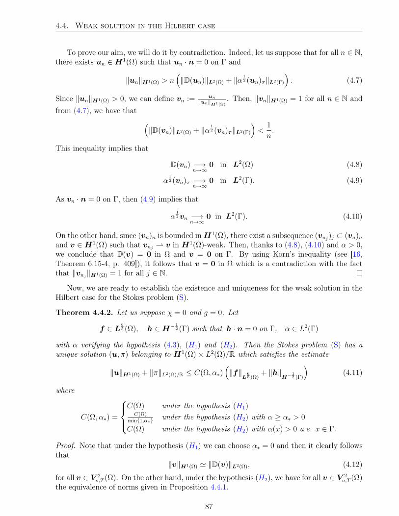
4.4. Weak solution in the Hilbert case

To prove our aim, we will do it by contradiction. Indeed, let us suppose that for all n ∈ N,there exists un ∈H1(Ω) such that un · n = 0 on Γ and

‖un‖H1(Ω) > n(‖D(un)‖L2(Ω) + ‖α

12 (un)τ‖L2(Γ)

). (4.7)

Since ‖un‖H1(Ω) > 0, we can define vn := un‖un‖H1(Ω)

. Then, ‖vn‖H1(Ω) = 1 for all n ∈ N andfrom (4.7), we have that (

‖D(vn)‖L2(Ω) + ‖α12 (vn)τ‖L2(Γ)

)<

1

n.

This inequality implies that

D(vn) −→n→∞

0 in L2(Ω) (4.8)

α12 (vn)τ −→

n→∞0 in L2(Γ). (4.9)

As vn · n = 0 on Γ, then (4.9) implies that

α12vn −→

n→∞0 in L2(Γ). (4.10)

On the other hand, since (vn)n is bounded inH1(Ω), there exist a subsequence (vnj)j ⊂ (vn)nand v ∈H1(Ω) such that vnj v in H1(Ω)-weak. Then, thanks to (4.8), (4.10) and α > 0,we conclude that D(v) = 0 in Ω and v = 0 on Γ. By using Korn’s inequality (see [16,Theorem 6.15-4, p. 409]), it follows that v = 0 in Ω which is a contradiction with the factthat ‖vnj‖H1(Ω) = 1 for all j ∈ N.

Now, we are ready to establish the existence and uniqueness for the weak solution in theHilbert case for the Stokes problem (S).

Theorem 4.4.2. Let us suppose χ = 0 and g = 0. Let

f ∈ L65 (Ω), h ∈H−


with α verifying the hypothesis (4.3), (H1) and (H2). Then the Stokes problem (S) has aunique solution (u, π) belonging to H1(Ω)× L2(Ω)/R which satisfies the estimate

‖u‖H1(Ω) + ‖π‖L2(Ω)/R ≤ C(Ω, α∗)(‖f‖

L65 (Ω)

+ ‖h‖H−

12 (Γ)

)(4.11)

where

C(Ω, α∗) =




Proof. Note that under the hypothesis (H1) we can choose α∗ = 0 and then it clearly followsthat

‖v‖H1(Ω) ' ‖D(v)‖L2(Ω), (4.12)

for all v ∈ V 2σ,T (Ω). On the other hand, under the hypothesis (H2), we have for all v ∈ V 2

σ,T (Ω)the equivalence of norms given in Proposition 4.4.1.

87


It follows that the existence of the unique solution (u, π) ∈ H1(Ω) × L2(Ω)/R is aconsequence of the Lax-Milgram theorem (because from above we can prove the coercivityof the bilinear form associated to the variational formulation (4.4)) besides the De Rham’stheorem (to recover the pressure), see Remark 4.3.6.

The estimate follows from the fact that the solution u verifies

2

∫Ω

|D(u)|2 dx+

∫Γ

α|uτ |2 ds ≤ ‖f‖L

65 (Ω)‖u‖L6(Ω) + ‖h‖

H−12 (Γ)‖u‖

H12 (Γ)

,

that is, if α satisfies (H1) or (H2) with α ≥ α∗ > 0, then

2‖D(u)‖2L2(Ω) + α∗‖uτ‖2

L2(Γ) ≤ ‖f‖L 65 (Ω)‖u‖L6(Ω) + ‖h‖

H−12 (Γ)‖u‖

H12 (Γ)

,

and if α satisfies (H2) with α(x) > 0 a.e. x ∈ Γ, then

‖D(u)‖2L2(Ω) + ‖α

12uτ‖2

L2(Γ) ≤ ‖f‖L 65 (Ω)‖u‖L6(Ω) + ‖h‖

H−12 (Γ)‖u‖

H12 (Γ)

.

In this way, if α satisfies (H1), we can choose α∗ = 0, and from (4.12) we obtain that

‖u‖H1(Ω) ≤ C1(Ω)(‖f‖

L65 (Ω)

+ ‖h‖H−

12 (Γ)

);

if α satisfies (H2) with α ≥ α∗ > 0, from (4.6), we have

‖u‖H1(Ω) ≤C2(Ω)

min1, α∗

(‖f‖

L65 (Ω)

+ ‖h‖H−

12 (Γ)

),

and if α satisfies (H2) with α(x) > 0 a.e. x ∈ Γ, from (4.5), it follows that

‖u‖H1(Ω) ≤ C3(Ω)(‖f‖

L65 (Ω)

+ ‖h‖H−

12 (Γ)

).

On the other hand,

‖π‖L2(Ω)/R ≤ ‖∇π‖H−1(Ω)

≤ C4(Ω)(‖f‖

L65 (Ω)

+ ‖∆u‖H−1(Ω)

)≤ C4(Ω)

(‖f‖

L65 (Ω)

+ ‖u‖H1(Ω)

).

Hence,‖π‖L2(Ω)/R ≤ C4(Ω)

(‖f‖

L65 (Ω)

+ ‖h‖H−

12 (Γ)

). (4.13)

The estimate (4.11) follows immediately from the estimates for u in each case and (4.13).

Remark 4.4.3. (i) In the case α(x) > 0 a.e. x ∈ Γ, we have another equivalence of normsfor the velocity field thanks to Proposition 3.3.8: for all u ∈ V 2

σ,T (Ω)

‖u‖H1(Ω) ' ‖D(u)‖L2(Ω).

(ii) The case α = 0 and Ω axisymmetric is analyzed in [5].

88


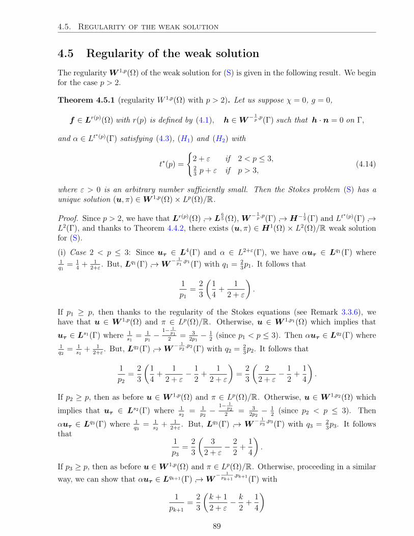
4.5 Regularity of the weak solution

The regularityW 1,p(Ω) of the weak solution for (S) is given in the following result. We beginfor the case p > 2.

Theorem 4.5.1 (regularity W 1,p(Ω) with p > 2). Let us suppose χ = 0, g = 0,


and α ∈ Lt∗(p)(Γ) satisfying (4.3), (H1) and (H2) with

t∗(p) =

2 + ε if 2 3,

(4.14)

where ε > 0 is an arbitrary number sufficiently small. Then the Stokes problem (S) has aunique solution (u, π) ∈W 1,p(Ω)× Lp(Ω)/R.

Proof. Since p > 2, we have that Lr(p)(Ω) → L65 (Ω),W− 1

p,p(Γ) →H−

12 (Γ) and Lt∗(p)(Γ) →

L2(Γ), and thanks to Theorem 4.4.2, there exists (u, π) ∈ H1(Ω) × L2(Ω)/R weak solutionfor (S).

(i) Case 2 < p ≤ 3: Since uτ ∈ L4(Γ) and α ∈ L2+ε(Γ), we have αuτ ∈ Lq1(Γ) where1q1

= 14

+ 12+ε

. But, Lq1(Γ) →W− 1p1,p1(Γ) with q1 = 2

3p1. It follows that

1

p1

=2

3

(1

4+

1

2 + ε

).

If p1 ≥ p, then thanks to the regularity of the Stokes equations (see Remark 3.3.6), wehave that u ∈ W 1,p(Ω) and π ∈ Lp(Ω)/R. Otherwise, u ∈ W 1,p1(Ω) which implies that

uτ ∈ Ls1(Γ) where 1s1

= 1p1−

1− 1p1

2= 3

2p1− 1

2(since p1 < p ≤ 3). Then αuτ ∈ Lq2(Γ) where

1q2

= 1s1

+ 12+ε

. But, Lq2(Γ) →W− 1p2,p2(Γ) with q2 = 2

3p2. It follows that

1

p2

=2

3

(1

4+

1

2 + ε− 1

2+

1

2 + ε

)=

2

3

(2

2 + ε− 1

2+

1

4

).

If p2 ≥ p, then as before u ∈ W 1,p(Ω) and π ∈ Lp(Ω)/R. Otherwise, u ∈ W 1,p2(Ω) which

implies that uτ ∈ Ls2(Γ) where 1s2

= 1p2−

1− 1p2

2= 3

2p2− 1

2(since p2 < p ≤ 3). Then

αuτ ∈ Lq3(Γ) where 1q3

= 1s2

+ 12+ε

. But, Lq3(Γ) → W− 1p3,p3(Γ) with q3 = 2

3p3. It follows

that1

p3

=2

3

(3

2 + ε− 2

2+

1

4

).

If p3 ≥ p, then as before u ∈W 1,p(Ω) and π ∈ Lp(Ω)/R. Otherwise, proceeding in a similarway, we can show that αuτ ∈ Lqk+1(Γ) →W

− 1pk+1

,pk+1(Γ) with

1

pk+1

=2

3

(k + 1

2 + ε− k

2+

1

4

)89


(in order to get this, we use the fact that pk < 3). Then, u ∈ W 1,pk+1(Ω) and choosingk = b1

ε− 1

2c + 1 (where bac stands for the greatest integer less than or equal to a) we have

that pk+1 ≥ 3 ≥ p. Finally u ∈W 1,p(Ω) and π ∈ Lp(Ω)/R.

(ii) Case p > 3: From the previous case, we have that (u, π) ∈ W 1,3(Ω) × L3(Ω). Thisimplies that uτ ∈ Lq(Γ) for all 1 < q < ∞, and since α ∈ L

2p3

+ε(Γ), we obtain thatαuτ ∈ L

2p3 (Γ) →W− 1

p,p(Γ). Finally, by using the regularity of the Stokes equations (Remark

3.3.6), we have that u ∈W 1,p(Ω) and π ∈ Lp(Ω).

Remark 4.5.2. (i) The regularity W 1,p(Ω) when α = 0 is given in [5].(ii) Note that for p > 3, we can not consider α ∈ Ls(Γ) with s ≤ 2 + ε. Indeed, let ussuppose that α ∈ L2+ε(Γ) and since uτ ∈ Lq(Γ) for 1 < q <∞, we have that αuτ ∈ L2(Γ).Then, we have L2(Γ) → W− 1

p,p(Γ) if and only if p ≤ 3, which is not the case.

(iii) We will study later the case of generalized solutions in W 1,p(Ω)× Lp(Ω) for p < 2.

Now, we study the case of strong solutions for the Stokes problem (S).

Theorem 4.5.3 (regularity W 2,p(Ω) with p ≥ 65). Let us suppose χ = 0, g = 0,


and

α ∈ H12 (Γ) if

6

5≤ p ≤ 2; α ∈ H

12

+ε(Γ) if 2 0 is an arbitrary number sufficiently small and α satisfies (4.3), (H1) and (H2).Then the solution given by Theorem 4.4.2 satisfies that (u, π) ∈W 2,p(Ω)×W 1,p(Ω)/R.

Proof. Due to p ≥ 65, it follows that Lp(Ω) → L

65 (Ω),W 1− 1

p,p(Γ) →H−

12 (Γ) and α ∈ L2(Γ),

then thanks to Theorem 4.4.2, there exists (u, π) ∈H1(Ω)×L2(Ω)/R weak solution for (S).

(i) Case 65≤ p ≤ 2: Since α ∈ H 1

2 (Γ), we can extend α to the inside of the domain Ω, hencewe can consider α ∈ H1(Ω). Then, for all i, j = 1, 2, 3 we have that ∂α

∂xjui ∈ Lq1(Ω) and

α ∂ui∂xj∈ Lq1(Ω) where 1

q1= 1

2+ 1

6= 2

3. Then, ∂

∂xj(αui) = ∂α

∂xjui + α ∂ui

∂xj∈ L 3

2 (Ω) which implies

that αu ∈W 1, 32 (Ω) and therefore, αuτ ∈W 1− 2

3, 32 (Γ). By using Proposition 3.3.3, we have

that u ∈W 2, 32 (Ω) and π ∈W 1, 3

2 (Ω)/R.From above we have that u ∈ W 2, 3

2 (Ω) → Ls(Ω) for all 1 < s < ∞ and ∇u ∈W 1, 3

2 (Ω) → L3(Ω). Then, for all i, j = 1, 2, 3 we have that ∂α∂xjui ∈ Lq2(Ω) where 1

q2= 1

2+ 1

s

and α ∂ui∂xj∈ Lq3(Ω) where 1

q3= 1

6+ 1

3= 1

2. Clearly, q2 < q3 and then ∂

∂xj(αui) ∈ Lq2(Ω) which

implies that αu ∈W 1,q2(Ω) and therefore, αuτ ∈W 1− 1q2,q2(Γ). By using Proposition 3.3.3,

we have that u ∈W 2,q2(Ω) and π ∈ W 1,q2(Ω)/R with 32< q2 < 2.

Finally, since u ∈W 2,q2(Ω) → L∞(Ω) and ∇u ∈W 1,q2(Ω) → Lq∗2 (Ω) with 1

q∗2= 1

q2− 1

3,

we have for all i, j = 1, 2, 3 that ∂α∂xjui ∈ L2(Ω) and α ∂ui

∂xj∈ Lq4(Ω) where 1

q4= 1

6+ 1

q∗2= 1

q2− 1

6.

Clearly, 2 < q4 and then ∂∂xj

(αui) ∈ L2(Ω) which implies that αu ∈ H1(Ω) and therefore,

αuτ ∈ H12 (Γ). By using Proposition 3.3.3, we have that u ∈ H2(Ω) and π ∈ H1(Ω)/R.

Then, we have showed that (u, π) ∈W 2,p(Ω)×W 1,p(Ω)/R for 65≤ p ≤ 2.

90


(ii) Case 2 < p < 3: From the previous case, we have that (u, π) ∈ H2(Ω) × H1(Ω),hence, u ∈ L∞(Ω) and ∇u ∈ H1(Ω) → L6(Ω). Since α ∈ H

12

+ε(Γ), we can regardα ∈ H1+ε(Ω) → Ls(Ω) where 1

s= 1

2− 1+ε

3, assuming that ε < 1

2. Also, ∇α ∈Hε(Ω) → Lt(Ω)

where 1t

= 12− ε

3. For all i, j = 1, 2, 3 we have that ∂α

∂xjui ∈ Lt(Ω) and α ∂ui

∂xj∈ Lr(Ω) where

1r

= 1s+ 1

6= 1

3− ε

3. Clearly, t < r and then ∂

∂xj(αui) ∈ Lt(Ω) which implies that αu ∈W 1,t(Ω)

and therefore, αuτ ∈W 1− 1t,t(Γ) where 2 < t < 3. By using Proposition 3.3.3, we have that

u ∈W 2,t(Ω) and π ∈ W 1,t(Ω)/R. Then, (u, π) ∈W 2,p(Ω)×W 1,p(Ω)/R for 2 < p < 3.(ii) Case p ≥ 3: From above we have that u ∈ W 2,t(Ω) for 2 < t < 3, hence, u ∈ L∞(Ω)

and ∇u ∈ W 1,t(Ω) → Lr(Ω) where 1r

= 1t− 1

3. Since α ∈ W 1− 1

p,p(Γ), we can regard

α ∈ W 1,p(Ω) → Ls(Ω) where 1 < s < ∞ for p = 3 and s = ∞ for p > 3. Further,∇α ∈ Lp(Ω).

If p = 3, then for all i, j = 1, 2, 3 we have that ∂α∂xjui ∈ L3(Ω) and α ∂ui

∂xj∈ Lr∗(Ω) where

1r∗

= 1s

+ 1rfor any 1 < s <∞, then 1

r∗= 1

s+ 1

2− ε

3− 1

3= 1

s+ 1

6− ε

3. Choosing s sufficiently

big such that s − ε3≤ 0, we have that r∗ ≥ 6. Clearly, 3 < r∗ and then ∂

∂xj(αui) ∈ L3(Ω)

which implies that αu ∈ W 1,3(Ω) and therefore, αuτ ∈ W 1− 13,3(Γ). By using Proposition

3.3.3, we have that u ∈W 2,3(Ω) and π ∈ W 1,3(Ω)/R.On the other hand, if p > 3, we have u ∈ W 2,3(Ω) → L∞(Ω) and ∇u ∈ W 1,3(Ω) →

Ls∗(Ω) for any 1 < s∗ <∞. Further, α ∈ L∞(Ω) and ∇α ∈ Lp(Ω). Then, for all i, j = 1, 2, 3

we have that ∂α∂xjui ∈ Lp(Ω) and α ∂ui

∂xj∈ Ls∗(Ω). For s∗ sufficiently large, we have that p ≤ s∗.

It follows that ∂∂xj

(αui) ∈ Lp(Ω) which implies that αu ∈ W 1,p(Ω) and therefore, αuτ ∈W 1− 1

p,p(Γ). By using Proposition 3.3.3, we have that u ∈W 2,p(Ω) and π ∈ W 1,p(Ω)/R.

Remark 4.5.4. (i) The regularity W 2,p(Ω) when α = 0 is given in [5].(ii) We will study later the case of strong solutions in W 2,p(Ω)×W 1,p(Ω) for 1 < p < 6

5.

91

Bibliography

[1] P. Acevedo, C. Amrouche, and C. Conca. Existence, uniqueness and regularity for theBoussinesq system with non-homogeneous boundary conditions. Submitted for publica-tion.

[2] H. Al Baba. Problèmes d’évolutions de Stokes et de Navier-Stokes avec des conditionsaux limites de type Navier. PhD thesis, Université de Pau et des Pays de l’Adour, 2015.

[3] C. J. Amick. Existence of solutions to the nonhomogeneous steady Navier-Stokes equa-tions. Indiana Univ. Math. J., 33(6):817–830, 1984.

[4] C. Amrouche and V. Girault. Decomposition of vector spaces and application to theStokes problem in arbitrary dimension. Czechoslovak Math. J., 44(1):109–140, 1994.

[5] C. Amrouche and A. Rejaiba. Lp-theory for Stokes and Navier–Stokes equations withNavier boundary condition. J. Differential Equations, 256(4):1515–1547, 2014.

[6] C. Amrouche and M. A. Rodríguez-Bellido. Stationary Stokes, Oseen and Navier-StokesEquations with Singular Data. Arch. Ration. Mech. Anal., 199(2):597–651, 2011.

[7] C. Amrouche and N. Seloula. Lp-theory for vector potentials and Sobolev’s inequalitiesfor vector fields: Application to the Stokes equations with pressure boundary conditions.Math. Models Methods Appl. Sci., 23(1):37–92, 2013.

[8] C. Bègue, C. Conca, F. Murat, and O. Pironneau. Les équations de Stokes et de Navier-Stokes avec des conditions aux limites sur la pression. In Nonlinear Partial DifferentialEquations and their Applications, Collège de France Seminar, volume 9, pages 179–264.Pitman Res. Notes Math. Ser., 1988.

[9] H. Beirão da Veiga. Regularity for Stokes and generalized Stokes systems under non-homogeneous slip-type boundary conditions. Adv. Differential Equations, 9(9-10):1079–1114, 2004.

[10] C. Bernardi, B. Métivet, and B. Pernaud-Thomas. Couplage des équations de Navier-Stokes et de la chaleur: le modèle et son approximation par éléments finis. RAIROModél. Math. Anal. Numér., 29(7):871–921, 1995.

[11] L. Berselli and S. Spirito. An elementary approach to the inviscid limits for the 3DNavier–Stokes equations with slip boundary conditions and applications to the 3DBoussinesq equations. NoDEA Nonlinear Differential Equations Appl., 21(2):149–166,2014.

92

Bibliography

[12] W. Borchers and K. Pileckas. Note on the flux problem for stationary incompressibleNavier-Stokes equations in domains with a multiply connected boundary. Acta Appl.Math., 37(1-2):21–30, 1994.

[13] J. Boussinesq. Théorie analytique de la chaleur: mise en harmonie avec la thermody-namique et avec la théorie mécanique de la lumière, volume 2. Gauthier-Villars, Paris,1903.

[14] J. Casado-Díaz, E. Fernández-Cara, and J. Simon. Why viscous fluids adhere to rugosewalls: A mathematical explanation. J. Differential Equations, 189(2):526–537, 2003.

[15] S. Chandrasekhar. Hydrodynamic and Hydromagnetic Stability. The International Seriesof Monographs on Physics. Clarendon Press, Oxford, 1961.

[16] P. G. Ciarlet. Linear and Nonlinear Functional Analysis with Applications. AppliedMathematics. SIAM, 2013.

[17] C. Conca. Numerical results on the homogenization of Stokes and Navier-Stokes equa-tions modeling a class of problems from fluid mechanics. Comput. Methods Appl. Mech.Engrg., 53(3):223–258, 1985.

[18] C. Conca. On the application of the homogenization theory to a class of problems arisingin fluid mechanics. J. Math. Pures Appl., 64(1):31–75, 1985.

[19] C. Conca. Stokes equations with non-smooth data. Rev. Mat. Apl., 10(2):115–122, 1989.

[20] C. Conca, F. Murat, and O. Pironneau. The Stokes and Navier-Stokes equations withboundary conditions involving the pressure. Japan. J. Math., 20(2):279–318, 1994.

[21] L. Consiglieri, Š. Necasová, and J. Sokolowski. Incompressible Maxwell-Boussinesqapproximation: Existence, uniqueness and shape sensitivity. Control Cybernet.,38(4A):1193–1215, 2009.

[22] P. De Boer. Thermally driven motion of strongly heated fluids. Int. J. Heat MassTransfer, 27(12):2239–2251, 1984.

[23] L. Desvillettes and C. Villani. On a variant of Korn’s inequality arising in statisticalmechanics. ESAIM Control Optim. Calc. Var., 8:603–619, 2002.

[24] R. Dmowska and B. Saltzman. Advances in Geophysics, volume 33 of ADVANCES INGEOPHYSICS. Academic Press, 1991.

[25] P. Drazin and W. Reid. Hydrodynamic stability. Cambridge university press, 2004.

[26] R. Farwig and H. Morimoto. Leray’s Inequality for Fluid Flow in Symmetric Multi-connected Two-dimensional Domains. Tokyo J. Math., 35(1):63–70, 2012.

[27] G. P. Galdi. An Introduction to the Mathematical Theory of the Navier-Stokes Equations:Steady-State Problems. Springer Monographs in Mathematics. Springer, New York, 2ndedition, 2011.

93

Bibliography

[28] M. I. Gil’. Solvability of a system of stationary Boussinesq equations. Differ. Equ.,27(11):1377–1382, 1991.

[29] D. Gilbarg and N. S. Trudinger. Elliptic Partial Differential Equations of Second Order.Springer-Verlag, Berlin, 2001.

[30] V. Girault and P. A. Raviart. Finite Element Methods for Navier-Stokes Equations:Theory and Algorithms. Springer Series in Computational Mathematics, 5. Springer-Verlag, Berlin, 1986.

[31] D. Gray and A. Giorgini. The validity of the Boussinesq approximation for liquids andgases. Int. J. Heat Mass Transfer, 19(5):545–551, 1976.

[32] V. John. Slip with friction and penetration with resistance boundary conditions forthe Navier-Stokes equations — numerical tests and aspects of the implementation. J.Comput. Appl. Math., 147(2):287–300, 2002.

[33] D. D. Joseph. Stability of Fluid Motions II. Springer Tracts in Natural Philosophy.Springer-Verlag, 1976.

[34] J. P. Kelliher. Navier-Stokes Equations with Navier Boundary Conditions for a BoundedDomain in the Plane. SIAM J. Math. Anal., 38(1):210–232, 2006.

[35] H. Kim. The existence and uniqueness of very weak solutions of the stationary Boussi-nesq system. Nonlinear Anal., 75(1):317–330, 2012.

[36] H. Kozono and T. Yanagisawa. Leray’s problem on the stationary Navier–Stokes equa-tions with inhomogeneous boundary data. Math. Z., 262(1):27–39, 2009.

[37] P. K. Kundu, I. M. Cohen, and D. R. Dowling. Fluid Mechanics. Elsevier, 5th edition,2012.

[38] G. N. Kuraev. The problem of stationary free convection with non-linear boundaryconditions. U.S.S.R. Comput. Math. and Math. Phys., 18(3):263–270, 1978.

[39] O. A. Ladyzhenskaya. The Mathematical Theory of Viscous Incompressible Flow, vol-ume 2 of Mathematics and Its Applications. Gordon and Breach, Science Publishers,New York, 2nd edition, 1969.

[40] J. Leray. Étude de diverses équations intégrales non linéaires et de quelques problèmesque pose l’hydrodynamique. J. Math. Pures Appl., 12:1–82, 1933.

[41] A. Liakos. Discretization of the Navier-Stokes equations with slip boundary condition.Numer. Methods Partial Differential Equations, 17(1):26–42, 2001.

[42] A. Liakos. Discretization of the Navier-Stokes equationswith slip boundary condition II.Comput. Math. Appl., 48(7):1153–1166, 2004.

[43] J. L. Lions. Quelques Méthodes de Résolution des Problèmes aux Limites Non Linéaires.Dunod, Paris, 1969.

94

Bibliography

[44] J. C. Maxwell. On Stresses in Rarified Gases Arising from Inequalities of Temperature.Philosophical Transactions of the Royal Society of London, 170:pp. 231–256, 1879.

[45] T. McDougall, R. Greatbatch, and Y. Lu. On conservation equations in oceanogra-phy: How accurate are Boussinesq ocean models? Journal of Physical Oceanography,32(5):1574–1584, 2002.

[46] J. M. Mihaljan. A Rigorous Exposition of the Boussinesq Approximations Applicableto a Thin Layer of Fluid. Astrophys. J., 136:1126–1133, 1962.

[47] H. Morimoto. On the existence of weak solutions of equation of natural convection. J.Fac. Sci. Univ. Tokyo Sect. IA Math., 36:87–102, 1989.

[48] H. Morimoto. On the existence and uniqueness of the stationary solution to the equationsof natural convection. Tokyo J. Math., 14(1):217–226, 1991.

[49] H. Morimoto. A Remark on the Existence of 2-D Steady Navier–Stokes Flow in BoundedSymmetric Domain Under General Outflow Condition. J. Math. Fluid Mech., 9(3):411–418, 2007.

[50] H. Morimoto. Heat convection equation with nonhomogeneous boundary condition.Funkcial. Ekvac., 53(2):213–229, 2010.

[51] C. Navier. Mémoire sur les lois du mouvement des fluides. Mémoires de l’AcadémieRoyale des Sciences de l’Institut de France, 6:389–440, 1823.

[52] E. A. Notte-Cuello and M. A. Rojas-Medar. Stationary solutions for generalized Boussi-nesq models in exterior domains. Electron. J. Differential Equations, 1998(22):1–9, 1998.

[53] A. Novotný, M. Ruzicka, and G. Thäter. Rigorous derivation of the anelastic approxi-mation to the Oberbeck-Boussinesq equations. Asymptot. Anal., 75(1-2):93–123, 2011.

[54] A. Oberbeck. Ueber die Wärmeleitung der Flüssigkeiten bei Berücksichtigung der Strö-mungen infolge von Temperaturdifferenzen. Annalen der Physik, 243(6):271–292, 1879.

[55] A. Oberbeck. Über die Bewegungserscheinungen der Atmosphaere. 1888.

[56] K. Oeda. Stationary solutions of the heat convection equations in exterior domains.Proc. Japan Acad. Ser. A Math. Sci., 73(6):111–115, 1997.

[57] J. R. A. Pearson. On convection cells induced by surface tension. J. Fluid Mech.,4:489–500, 1958.

[58] V. V. Pukhnachev. Viscous flows in domains with a multiply connected boundary. Adv.Math. Fluid Mech., pages 333–348, 2010.

[59] L. Rayleigh. LIX. On convection currents in a horizontal layer of fluid, when the highertemperature is on the under side. The London, Edinburgh, and Dublin PhilosophicalMagazine and Journal of Science, 32(192):529–546, 1916.

[60] M. Santos da Rocha, M. A. Rojas-Medar, and M. D. Rojas-Medar. On the existence anduniqueness of the stationary solution to equations of natural convection with boundarydata in L2. R. Soc. Lond. Proc. Ser. A Math. Phys. Eng. Sci., 459:609–621, 2003.

95

Bibliography

[61] M. Satoh. Atmospheric Circulation Dynamics and General Circulation Models. SpringerPraxis Books. Springer-Verlag Berlin Heidelberg, 2 edition, 2014.

[62] N. Seloula. Mathematical Analysis and Numerical Approximation of the Stokes andNavier-Stokes equations with non standard boundary conditions. PhD thesis, Universitéde Pau et des Pays de l’Adour, 2010.

[63] V. Solonnikov and V. Ščadilov. A certain boundary value problem for the stationarysystem of Navier-Stokes equations. Tr. Mat. Inst. Steklova, 125:196–210, 1973.

[64] E. A. Spiegel and G. Veronis. On the Boussinesq approximation for a compressible fluid.Astrophys. J., 131:442–447, 1960.

[65] G. G. Stokes. On some cases of fluid motion. Trans. Cambridge Phil. Soc., 8:105–165,1843.

[66] R. Temam. Navier-Stokes Equations: Theory and Numerical Analysis, volume 2 ofStudies in Mathematics and its Applications, 2. North-Holland, 1979.

[67] R. Verfürth. Finite element approximation on incompressible Navier-Stokes equationswith slip boundary condition. Numer. Math., 50(6):697–721, 1987.

[68] R. Verfürth. Finite element approximation of incompressible Navier-Stokes equationswith slip boundary condition II. Numer. Math., 59(1):615–636, 1991.

[69] E. H. Weber. Mikroskopische Beobachtungen sehr gesetzmässiger Bewegungen, welchedie Bildung von Niederschlägen harziger Körper aus Weingeist begleiten. Annalen derPhysik, 170(3):447–459, 1855.

[70] J.C. Weddell, J. Kwack, P.I. Imoukhuede, and A. Masud. Hemodynamic Analysis in anIdealized Artery Tree: Differences in Wall Shear Stress between Newtonian and Non-Newtonian Blood Models. PLoS One, 10(4):e0124575, 2015.

[71] J. Wesfreid. Scientific Biography of Henri Bénard (1874–1939). In Dynamics of Spatio-Temporal Cellular Structures, pages 9–37. Springer, 2006.

[72] A.M. Yaglom and U. Frisch. Hydrodynamic Instability and Transition to Turbulence.Fluid Mechanics and Its Applications. Springer Netherlands, 2012.

[73] R. Zeytounian. Joseph Boussinesq and his approximation: a contemporary view. C. R.Mecanique, 331(8):575–586, 2003.

[74] R. Zeytounian. Theory and Applications of Viscous Fluid Flows. Springer-Verlag BerlinHeidelberg, 2004.

96

Documents

L -THEORY FOR THE BOUSSINESQ SYSTEM PAUL ANDR ES …