Irregular wave propagation with a 2DH Boussinesq-type

HAL Id: hal-01419946https://hal.inria.fr/hal-01419946

Submitted on 20 Dec 2016

HAL is a multi-disciplinary open accessarchive for the deposit and dissemination of sci-entific research documents, whether they are pub-lished or not. The documents may come fromteaching and research institutions in France orabroad, or from public or private research centers.

L’archive ouverte pluridisciplinaire HAL, estdestinée au dépôt et à la diffusion de documentsscientifiques de niveau recherche, publiés ou non,émanant des établissements d’enseignement et derecherche français ou étrangers, des laboratoirespublics ou privés.

Irregular wave propagation with a 2DH Boussinesq-typemodel and an unstructured finite volume scheme

M Kazolea, A Delis

To cite this version:M Kazolea, A Delis. Irregular wave propagation with a 2DH Boussinesq-type model and an unstruc-tured finite volume scheme. [Research Report] RR-9008, Inria Bordeaux Sud-Ouest. 2016. hal-01419946

https://hal.inria.fr/hal-01419946

https://hal.archives-ouvertes.fr

ISS

N02

49-6

399

ISR

NIN

RIA

/RR

--90

08--

FR+E

NG

RESEARCHREPORTN° 9008December 2016

Project-Teams Cardamom

Irregular wavepropagation with a 2DHBoussinesq-type modeland an unstructuredfinite volume schemeM. Kazolea, A.I. Delis

RESEARCH CENTREBORDEAUX – SUD-OUEST

200 avenue de la Vieille Tour33405 Talence Cedex

Irregular wave propagation with a 2DHBoussinesq-type model and an unstructured finite

volume scheme

M. Kazolea*, A.I. Delis†

Project-Teams Cardamom

Research Report n° 9008 — December 2016 — 24 pages

Abstract: The application and validation, with respect to the transformation, breaking and run-up ofirregular waves, of an unstructured high-resolution finite volume (FV) numerical solver for the 2D extendedBoussinesq-type (BT) equations of Nwogu (1993) is presented. The numerical model is based on thecombined FV approximate solution of the BT model and that of the nonlinear shallow water equations(NSWE) when wave breaking emerges. The FV numerical scheme satisfies the desired properties of well-balancing, for flows over complex bathymetries and in presence of wet/dry fronts, and shock-capturing foran intrinsic representation of wave breaking, that is handled as a shock by the NSWE. Several simulationsand comparisons with experimental data show that the model is able to simulate wave height variations,mean water level setup, wave run-up, swash zone oscillations and the generation of near-shore currentswith satisfactory accuracy.

Key-words: Irregular Waves, Boussinesq-type equations, Finite Volumes, Unstructured meshes

This is a note

This is a second note

* Inria Bordeaux Sud-Ouest, 200 Avenue de la Vielle Tour, 33405 Talence cedex, France- [email protected]† School of Production Engineering and Management, Technical University of Crete, University Campus, Chania, Crete, Greece

Propagation des vagues irrégulières avec un modèle Boussinesq2DH et un schéma de volumes finis non-structurés

Résumé : On présente la validation d’un code Boussinesq non-structuré utilisant les equations de Nwogusur simulation de la transformation et du déferlement de vagues correspondantes à des états de mer ir-réguliers. Le code résout les equations de Boussinesq par une méthode de type Volumes Finis (VF) avecune approximation de type Shallow-Water dans les régions déferlantes. Le schéma VF utilisé est well-balanced pour des bathymétries arbitraires et en présence de fronts secs. Les propriétés de capture dechoc du schéma utilisé permettent aussi de représenter correctement les fronts déferlants par des ressauts,grace à l’utilisation locale des équations shallow water. La comparaison avec une large base de donnéesexpérimentales démontre le potentiel de l’approche proposée pour prédire avec une précision satisfaisanteles hauteurs d’eau, le setup, l’inondation et l’oscillation dans la région de swash.

Mots-clés : vagues irréguliers, equations de type Boussinesq, Volumes Finis, non-structuré

Irregular wave propagation with a 2DH BT model 3

1 Introduction

Accurate simulations of near-shore hydrodynamics is of fundamental importance to marine and coastalengineering. Wind and swell gravity water waves propagate towards the coastline in groups of high- andlow-frequency waves which shoal in shallow waters and eventually break on the beach. As such, near-shore hydrodynamics are strongly influenced by the evolution of both high- and low-frequency wavesand their interactions. Due to their dispersive nature, these wave groups are transient and evolve in spaceand time leading to wave focusing that can potentially result to the formation of extreme or rogue waves.In addition to the formation of extreme waves, the focusing of wave energy, along with the wave heightvariation across the group, forces low-frequency long waves that propagate with the wave group. Thesegroup bound long waves may be amplified by continued forcing during shoaling of the short-wave groupsin shallower water. In sufficiently shallow water, the short waves within the group break at differentdepths, leading to further long-wave forcing by the varying breakpoint position. The influence of low-frequency waves on the short wave field is important, as it has been suggested that their presence mightlead to the de-saturation of the surf zone at short wave frequencies. Furthermore, low-frequency motions,which contribute significantly to surf and swash zone energy levels, are relevant to sediment mobility,harbor oscillations, and coastal inundation.

Important physical effects associated with nonlinear transformations of sea waves in near-shore re-gions can be described by Boussinesq-type equations (BTE). BTE are more appropriate for describingflows in deeper waters where frequency dispersion effects may become more important than nonlinearityby introducing dispersion terms in the modeling thus being more suitable in waters where dispersion be-gins to have an effect on the free surface. Over the last decades, BTE have been widely used to describewave transformations in coastal regions. For very recent comprehensive reviews on the theory, numer-ics and applications of BT models we refer to the review works in [8, 24]. The success of the BTEs ismainly due to the optimal blend of physical adequacy, in representing all main physical phenomena, andto their relative computational ease. However, the accurate and efficient numerical approximation of BTequations is still in the focus of on-going research especially in terms of higher-order numerics and theadaptive mathematical/numerical description of the flow. The first set of extended BTE was derived byPeregrine [34], under the assumption that nonlinearity and frequency dispersion are weak and they arelimited to relatively shallow water due to the weak dispersion. Subsequent attempts to extent the validityand applicability of these so-called standard Boussinesq equations have been successful. Madsen andSorensen [29] and Nwogu [33] have extended their validity by giving a more accurate representation ofthe phase and group velocities in intermediate waters, closely relating to linear wave theory. Furthermore,significant effort has been made in recent years into advancing the nonlinear and dispersive properties ofBT models by including high order nonlinear and dispersion terms, we refer to [24] and references therein,which in turn are more difficult to integrate and thus require substantially more computational effort intheir numerical integration. Further, the correct representation of the low-frequency wave generation andevolution is a requirement for near-shore simulation models. To this end, the achievement of a good mod-eling of low-frequency motion is closely related to an accurate simulation of nonlinear energy transfers,breaking-induced energy dissipation and swash zone motion; hence, an appropriate treatment of the wavebreaking and wave run-up/run-down processes is very important.

The present work is complementary to [21, 22] where, for the first time, a high-order well-balancedunstructured finite volume (FV) scheme on triangular meshes was presented for modeling weakly non-linear and weakly dispersive water waves over slowly varying bathymetries, as described by the 2Ddepth-integrated BTE of Nwogu [33]. The FV scheme numerically solves the conservative form of theequations following the median dual node-centered approach, for both the advective and dispersive partof the equations. For the advective fluxes, the scheme utilizes an approximate Riemann solver along witha well-balanced topography source term upwinding. Higher order accuracy in space and time is achievedthrough a MUSCL-type reconstruction technique and through a strong stability preserving explicit Runge-

RR n° 9008

4 Kazolea & Delis

Kutta time stepping. The model aims at combining the best features of the two families of equations: thepropagation properties of Boussinesq equations and the shock-capturing features of the NSWE. At thispurpose, it solves Boussinesq equations where nonlinear and dispersive effects are both relevant andNSWE where nonlinearity prevails and dispersion is negligible. To this end, a new methodology waspresented in [22] to handle wave breaking over complex bathymetries in extended two-dimensional BTmodels. Certain criteria, along with their proper implementation, were established to characterize break-ing waves. Once breaking waves are recognized, a switching is performed locally in the computationaldomain from the BTE to NSWE by suppressing the dispersive terms in the vicinity of the wave fronts.Thus, the shock-capturing features of the FV scheme enable an intrinsic representation of the breakingwaves, which are handled as shocks by the NSWE. An additional methodology was presented on howto perform a stable switching between the BTE and NSWE within the unstructured FV framework Theproposed approach is essential and has been proven efficient, especially in two dimensional conditions,for regular wave propagation. Since the model is intended for practical, engineering purposes it aimsat accurately simulating the global effects of wave-breaking i.e. wave height decay, mean water levelsetup, current generation. Hence, the proposed model’s its application and validation, with respect to thetransformation, breaking and run-up of irregular waves is the main scope of this presentation

2 Mathematical ModelThe model equations solved in the present work, following [21, 22], are the extended BT equations ofNwogu [33] which describe weakly non-linear weakly dispersive water waves in variable bathymetries.They were derived under the assumption that the wave height (A) to constant water depth (h) ratio, ε :=A/h, which measures the weight of nonlinear effects, and the square water depth to wave length (L) ratioµ2 := h2/L2, which represents the dimension of the dispersive effects, is of the same order with, i.e.the Stokes number S := ε/µ2 = O(1). The equations provide accurate linear dispersion and shoalingcharacteristics for values of kh up to 3 (intermediate water depths), where k is the wave number and khis essentially a scale of the value of µ, providing a correction of O(µ2) to the shallow water theory. Byretaining O(µ2) terms in the derivation of the models some vertical variations in the horizontal velocityare included even though the explicit appearance of the vertical coordinate has been removed from thecontinuity and momentum equations by integration.

Using the velocity vector [u, v]T = u ≡ ua at an arbitrary distance, za, from the still water level, h, asthe velocity variable, an optimum value of za = −0.531h is derived so that the dispersion properties of theequations most closely approximate those defined by linear wave theory, making the equations applicableto a wider range of water depths compared to the classical Boussinesq equations. Following [21] thevector conservative form of the equations reads as:

∂tU + ∇ · H(U?) = S on Ω × [0, t] ⊂ R2 × R+, (1)

where Ω × [0, t] is the space-time Cartesian domain, U? = [H, qx, qy]T = [H,Hu,Hv]T are the physicallyconservative variables, with H being the total water depth and q = [qx, qy]T are the volume fluxes alongthe x and y directions, U is the vector of the actual solution variables and H = [F,G] the nonlinear fluxvectors given as

U =

HP1P2

, F =

qx

q2x/H +

12

gH2

qxqy/H

, G =

qy

qxqy/H

q2y/H +

12

gH2

,where

P =

[P1P2

]= H

[z2

a

2∇(∇ · u) + za∇(∇ · hu) + u

]. (2)

Inria


The source term vector, S = Sb + S f + Sd, includes the bed topography’s, b(x, y), slope Sb, the bed frictioneffects S f , and the dispersive terms Sd. These terms read as

Sb =

0−gH∂xb−gH∂yb

, Sd =

−ψc

−uψc + ψMx

−vψc + ψMy

.with

ψc = ∇ ·

[(z2

a

2−

h2

6

)h∇(∇ · u) +

(za +

h2

)h∇(∇ · hu)

], (3)

and

ψM =

[ψMx

ψMy

]= ∂tH

z2a

2∇(∇ · u) + ∂tHza∇(∇ · hu). (4)

The bed friction effects are approximated by the quadratic law:

S f =

0

−fw2

qx‖q‖h−2

−fw2

qy‖q‖h−2

where fw is the bed friction coefficient, typically in the range of O(10−3) to O(10−2), depending on theReynolds number and the bed material.

Equations (1) have flux terms identical as those in the NSW equations and variables P contain all timederivatives in the momentum equations, including part of the dispersion terms. The dispersion vector Sdcontains only spatial derivatives since ∂tH is explicitly defined by the mass equation. It is obvious that theNSW equations are a subset of the BT equations since equations (1) degenerate into the NSW equationswhen the dispersive terms in P and Sd are vanishing.

2.1 Wave generationThe internal generation of wave motion is performed following the approach of Wei et al. [51]. Themethod employs a source term added to the mass equation. This source function was obtained usingFourier transform and Green’s functions to solve the linearized and non-homogeneous equations of Pere-grine and Nwogu. In the present model, this source function wave making method is adopted in order tolet the reflected waves outgo through the wave generator freely.

To obtain a desired oscillation signal in the wave generating area, a source function S (x, t) is addedinto the mass conservation equation at each time step, which is expressed as

S (x, t) = D∗ exp(σ(x − xs)2

)sin(λy − ωt) (5)

in whichσ =

5(δL/4)2 =

80δ2L2 (6)

where L is the wave length, ω the wave frequency, θ the wave incident angle, λ(= ky = k sin θ) the wavenumber in the y−direction, xs is the location of the center of the wave-making area, δ is a parameter thatinfluences the width W = δL/2 of the wave generator area and D∗ is the source function’s amplitude. Fora monochromatic wave, D∗ is defined as

D∗ =2√σA0 cos θ

(ω2 − α1gk4h3

)ωk√π exp(−l2/4σ)

[1 − α(kh)2] (7)

RR n° 9008

6 Kazolea & Delis

where h is again the still water level at the wave generation region, A0 the wave amplitude, l(= kx =

k cos θ) the wave number in the x−direction, α = −0.390 and α1 = α + 1/3.For irregular waves and following [19] we use the linear superposition of component waves. Ac-

cording to the irregular wave concept of Longuet-Higgings et al. [27] the water surface elevation can bedescribed by

η(t) =

∞∑i=1

ai cos(ωit + εi)

where, ai andωi represent the amplitude and frequency of the component wave respectively and εi denotesthe initial phase of the component wave, which is distributed randomly in the range of [0, 2π] . This meansthat each component wave has its deterministic amplitude and frequency. The source function now readsas:

S (x, t) = exp(σ(x − xs)2

) M∑i=1

D∗i sin(λiy − ωit + εi) (8)

where the source function’s amplitude is now

D∗i =2√σAi cos θi

(ω2

i − α1gk4i h3

)ωki√π exp(−l2i /4σ)

[1 − α(kih)2] (9)

with li = ki sin(θi). For the wave making area W we use the maximum wavelength between the compo-nents.

The BT equations of Nwogu that we use in this work are restricted to h/L values less than 1/2.. Moreprecisely using a value of α = −0.39 in the range 0 < h/L < 1/2 gives an error of the normalised phasespeed of less than 2% [33]. Beyond this range errors in the linear dispersion relationship grow, hence oneshould be careful when testing to accurately represent the free waves at the given frequency. Following[47, 30] the wave generator is placed, each time, at the position with the appropriate water depth.

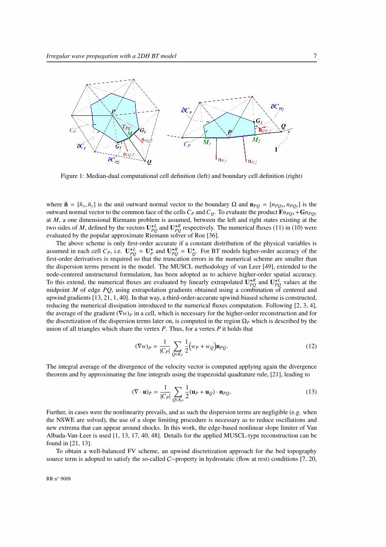
3 The Numerical MethodologyTo numerically solve BT system (1), the high-resolution shock-capturing finite volume (FV) scheme pro-posed in [21, 22] has been implemented. We will briefly review it here, for completeness. The consideredFV approach is of the vertex-centered median-dual type where the control volumes are elements dual to aprimal triangulation of the computational domain Ω. Referring to Fig. 1, the boundary ∂CP of a compu-tational cell CP, around an internal vertex P, is defined by connecting the barycenters of the surroundingtriangles with the mid-points of the corresponding edges that meet at vertex P.

After integration of (1) over each computational cell and application of the Gauss divergence theoremthe semi-discrete form of the scheme follows the usual FV formulation and reads as

∂UP

∂t= −

1|CP|

∑Q∈KP

F PQ −1|CP|F P,Γ +

1|CP|

∑Q∈KP

"CP.

S dΩ

, (10)

where UP is the volume-average value of the conserved-like quantities at a given time, KP is the set ofneighboring vertices to P, Γ is the boundary of Ω and F PQ and F P,Γ are the numerical flux vectors acrosseach internal and boundary face, respectively. Assuming a uniform distribution ofH over ∂CPQ, equal toits value at the midpoint M of edge PQ, these fluxes are approximated as

F PQ =

∮∂CPQ

(Fnx + Gny

)dl ≈

(Fnx + Gny

)M

∥∥∥nPQ

∥∥∥ =(FnPQx + GnPQy

)M. (11)

Inria


Figure 1: Median-dual computational cell definition (left) and boundary cell definition (right)

where n = [nx, ny] is the unit outward normal vector to the boundary Ω and nPQ = [nPQx, nPQy] is theoutward normal vector to the common face of the cells CP and CQ. To evaluate the product FnPQx +GnPQy

at M, a one dimensional Riemann problem is assumed, between the left and right states existing at thetwo sides of M, defined by the vectors U?L

PQ and U?RPQ respectively. The numerical fluxes (11) in (10) were

evaluated by the popular approximate Riemann solver of Roe [36].The above scheme is only first-order accurate if a constant distribution of the physical variables is

assumed in each cell CP, i.e. U?LPQ = U?

P and U?RPQ = U?

Q. For BT models higher-order accuracy of thefirst-order derivatives is required so that the truncation errors in the numerical scheme are smaller thanthe dispersion terms present in the model. The MUSCL methodology of van Leer [49], extended to thenode-centered unstructured formulation, has been adopted as to achieve higher-order spatial accuracy.To this extend, the numerical fluxes are evaluated by linearly extrapolated U?R

PQ and U?LPQ values at the

midpoint M of edge PQ, using extrapolation gradients obtained using a combination of centered andupwind gradients [13, 21, 1, 40]. In that way, a third-order-accurate upwind-biased scheme is constructed,reducing the numerical dissipation introduced to the numerical fluxes computation. Following [2, 3, 4],the average of the gradient (∇w)P in a cell, which is necessary for the higher-order reconstruction and forthe discretization of the dispersion terms later on, is computed in the region ΩP which is described by theunion of all triangles which share the vertex P. Thus, for a vertex P it holds that

(∇w)P =1|CP|

∑Q∈KP

12

(wP + wQ

)nPQ. (12)

The integral average of the divergence of the velocity vector is computed applying again the divergencetheorem and by approximating the line integrals using the trapezoidal quadrature rule, [21], leading to

(∇ · u)P =1|CP|

∑Q∈KP

12

(uP + uQ) · nPQ. (13)

Further, in cases were the nonlinearity prevails, and as such the dispersion terms are negligible (e.g. whenthe NSWE are solved), the use of a slope limiting procedure is necessary as to reduce oscillations andnew extrema that can appear around shocks. In this work, the edge-based nonlinear slope limiter of VanAlbada-Van-Leer is used [1, 13, 17, 40, 48]. Details for the applied MUSCL-type reconstruction can befound in [21, 13].

To obtain a well-balanced FV scheme, an upwind discretization approach for the bed topographysource term is adopted to satisfy the so-called C−property in hydrostatic (flow at rest) conditions [7, 20,

RR n° 9008

8 Kazolea & Delis

32]. To this end, the topography source term, Sb must be linearized in the same way and evaluated in thesame Roe-average states as the flux terms. More details can be found in [21, 22]. Moreover, in wet/dryfronts special considerations are needed to accurately model transition between wet and dry areas andmaintain the high-order spatial accuracy and mass conservation. As identified in [35, 13, 21], and webriefly list here for completeness, the following issues have are addressed:

• Dry cell identification. Computational cells with water depth H < εwd are considered as dry, whereεwd is a tolerance parameter computed from grid geometrical quantities [35, 13].

• Conservation of flow at rest with dry regions. A FV scheme has to satisfy the extended C-property[11]. We redefine the bed elevation at the emerging dry cell following [12, 9, 32, 13, 10] to obtainan exact balance at the front between the bed slope and the hydrostatic terms for steady conditions.

• Consisted depth reconstruction in dry regions. In a wet/wet steady case, in each computationalcell were the MUSCL reconstruction for b involves dry cells (∇H)P = −(∇b)P must be inforced tomaintain higher-order accuracy [13].

• Flow in motion over adverse slopes. For flow in motion and at wet/dry fronts we impose, temporar-ily, u = 0 for the computation of the numerical fluxes and source terms, following [11, 12, 32].

• Water depth positivity and mass conservation. To avoid computing negative water depths in dryingcells and to achieve absolute mass conservation, we follow treatments proposed in [9, 26, 13].

For the discretisation of the dispersion terms we assume a uniform distribution of the integratedquantities over ∂CPQ equal to their values at the midpoint M of the edge PQ. The mass equation in(1) contains the integral average of the dispersive term ψC and to approximate this term, we use thedivergence theorem, which leads to

(ψc)P ≈1|CP|

∑Q∈KP

[(z2

a

2−

h2

6

)h]

M

[∇(∇ · u) · nPQ

]M +

[(za +

h2

)h]

M

[∇(∇ · hu) · nPQ

]M

. (14)

In (14) we require the evaluation of the gradient of the divergence of u and hu along the edge midpoints M.Hence, the evaluation of the gradient of a quantity w at M requires the definition of a new computationalcell constructed by the union of the two triangles which share edge PQ. By denoting with KPQ :=R ∈ N | R is a vertex of MPQ

we obtain

(∇w)M =

"MPQ

∇wdΩ =

∮∂MPQ

wnRQdl =∑

R,Q∈KPQRQ∈∂MPQ

12

(wR + wQ

)nRQ, (15)

with nRQ the vector normal to the edge RQ.Next, for the the dispersive source terms in the momentum equations we have

1|CP|

"CP

−uψc + ψMdΩ = −uP

"CP

ψcdΩ +1|CP|

"CP

ψMdΩ. (16)

The first term of the right hand side of the equation is discretized as before in (14) and the second termtakes the discrete form:

(ψM)P =1|CP|

"CP

ψMdΩ =1|CP|

"CP

∂tHz2

a

2∇(∇ · u) + ∂tHza∇(∇ · hu)dΩ (17)

≈

[∂tH

z2a

2

]P|CP| [∇(∇ · u)]P + [∂tHza]P |CP| [∇(∇ · hu)]P ,

Inria


where the divergence (∇ · u)P and (∇ · hu)P are computed again using formula (12).Concerning the time discretization, an optimal third order explicit Strong Stability-Preserving Runge-

Kutta (SSP-RK) method was adopted [43, 21] under the usual CFL stability restriction. After each timestep in the RK scheme, the values of the velocities u = [u, v]T must be extracted from the new solutionvariable P = [P1, P2]T, from the momentum equation. The discretization of P results into a linear systemMV = C with M ∈ R2N×2N , V = [u1,u2, · · · uN]T and C = [P1,P2, · · ·PN]T. Matrix M is a sparse, meshdependent and structurally symmetric. Keeping in mind that u is our unknown velocity vector at eachmesh node, each two rows of the matrix correspond to a vertex P ∈ 1, 2, . . . ,N on the grid and for eachsuch vertex equation (2) holds. Using (12) to discretize equation (2) and replacing the arithmetic averagein equation (12) by the values at the midpoints M of the edges equation (2) reads as:

HP

(z2a)P

21|CP|

∑Q∈KP

(∇ · u)MnPQ +(za)P

|CP|

∑Q∈KP

(∇ · hu)MnPQ + uP

= PP. (18)

After some calculations the sparse 2N × 2N linear system to be solved can be presented in a compactform, as:

(z2a)P

2|CP|

∑Q∈KP

(AQuQ + APuP

)+

(za)P

|CP|

∑Q∈KP

(BQuQ + BPuP

)+ I2uP =

1HP

PP, P = 1 . . .N, (19)

where the sub-matrices AQ,AP,BQ,BP, depend only on the geometric quantities nPQ and area |MPQ|.The properties of the sparse matrix vary depending on the physical situation of each problem solved,

the type of the grid used and the number of the nodes on the grid. The matrix was stored in the compressedsparse row (CSR) format of and linear system was solved using the Bi-Conjugate Gradient Stabilizedmethod (BiCGStab) [38]. The ILUT pre-conditioner from SPARSKIT package [38] was implementedand the reverse Cuthill–McKee (RCM) algorithm [16] was also employed to reorder the matrix elementsas to minimize the matrix bandwidth. Convergence to the solution was obtained in one or two steps forthe test problems presented in following sections.

3.1 Wave breakingFor treating breaking waves the hybrid wave breaking model of Kazolea et al. [22] is implemented.This is a phase resolving model and up to now this treatment of breaking has only be tested on regularwaves [15, 22]. It is based on a hybrid BT/NSWE approach [22, 46] meaning that when a wave breakinginterface occurs, BTEs are turned into NSWE by switching off the dispersive terms. In this way, the wavebreaking interface is treated as a bore by the NSWE and the shock capturing FV scheme. The model isdescribed briefly below:

1. Using a new set of physical criteria we first estimate the location of breaking waves and then theNSWE are solved in the breaking regions and BTEs elsewhere. More precisely the criteria fortriggering the wave breaking modeling within the FV scheme are

• the surface variation criterion: |∂tη| ≥ γ√

gh

• the local slope angle criterion: ‖∇η‖2 ≥ tan(φc), where φc is the critical front face angle at theinitiation of breaking

The first criterion flags for breaking when ∂tη is positive, as breaking starts on the front face ofthe wave and has the advantage that can be easily calculated during the running of the model. Inprevious works [15, 22] which studied regular wave breaking over complex bathymetries the valueof γ varies from 0.35 to 0.65 and it may be affected by the scale of the wave under consideration.

RR n° 9008

10 Kazolea & Delis

Dealing with irregular wave breaking, it has been found, that these values are not affected. However,this criterion alone is inefficient for stably computing stationary (breaking or partially breaking)hydraulic jumps since in these cases ∂tη ≈ 0. The second criterion acts complementarily to thefirst one and is based on the critical front slope approach in [39, 41]. Depending on the BT modelused and the breaker type, e.g. spilling or plunging, the critical slope values are in the range ofφc ∈ [14o, 33o]. For certain BT models this has been considered as the least sensitive breakingthreshold, with the correct breaking location predicted for φc ≈ 30o, see for example [28, 44], andis is the value adopted in this work. This value for φc is relatively large for this criterion to triggerthe breaking process by its own in our BT model but is sufficient to detect breaking hydraulic jumpsthus, correcting the limitation of the first criterion.

2. If at least one of the criteria is satisfied: we flag the relative solution nodes as breaking ones in thecomputational mesh..

3. We distinguish the different breaking waves by creating a dynamical list that contains the breakingnodes of such a wave and the different breaking waves are treated individually.

4. The wave front of each breaking wave is then handled as a bore by the NSWE dissipating energy.At the same time, we take into account that bores stop breaking when their Froude (Fr) numberdrops below a critical value. If Fr 1 a bore is purely breaking and will consist of a steep frontand if the Fr number drops below a certain value Frc non-breaking undular bores occur, see [44].Thus, an additional criterion is needed to determine when to switch back to the BT equations fornon-breaking bores, allowing for the breaking process to stop. The criterion adopted is based on theanalogy between a broken wave and a bore in the sense of a simple transition between two uniformlevels. The wave’s Fr number is defined as:

Fr =

√(2H2/H1 + 1)2 − 1

8, (20)

where H1 is the water depth at the wave’s trough and H2 the water depth at the wave’s crest.Since we have tracked each breaking wave individually (with its own dynamic list), it is relativelystraightforward to find H1 and H2 for each wave. We simply approximate them by finding theminimum and maximum water depth respectively, from all the breaking nodes corresponding to thatwave. If Fr ≤ Frc all the breaking points of that wave are un-flagged and the wave is considerednon-breaking. Following [44, 22], the critical value for Frc was set equal to 1.3 in our computations.

5. For each breaking wave an extension of the computational region governed by the NSWE is per-formed, as to avoid non-physical effects that may appear at the interface between a zone governedby the BTEs and a zone governed by NSWE [22].

3.2 Boundary conditions

In the presented FV approach, the degrees of freedom are located directly on the physical boundary. Assuch, boundary conditions based on mesh faces rather than mesh vertices where adopted. To this end,the weak formulation was used where the boundary condition was introduced into the residual throughthe modified boundary flux F P,Γ in (5). The idea of using the weak formulation to calculate the flux(and dispersion terms) at the boundary has been used here in the description of wall (solid) boundaryconditions [21].

Absorbing boundaries have also been applied which should dissipate the energy of incoming wavesperfectly, in order to eliminate nonphysical reflections. In front of this kind of boundaries a sponge layer

Inria


is defined. On this layer, the surface elevation was damped by multiplying its value by a coefficient m(x)defined as [52]

m(x) =

√1 −

(x − d(x)

Ls

)2

(21)

where Ls is the sponge layer width and d(x) is the normal distance between the cell center with coordinatesx and the adsorbing boundary. The sponge layer width should be L ≤ Ls ≤ 1.5L, i.e. the width of thesponge layer is proportional to the wave length. Thus, longer wave lengths require longer sponge layers.

4 Numerical Tests and Results

4.1 Bichromatic wave groupsThe first test case reproduces the experiments made by Mase [31] on the transformation, breaking andrun-up of bichromatic wave groups on a mildly sloping beach. Mase’s laboratory measurements, whichinclude shoaling, breaking and swash motion, can provide good test cases for the verification of a run-upscheme in combination with a wave breaking model. Subsequently, these test cases have been used byresearchers, e.g. [47, 30, 23], to evaluate their numerical models.

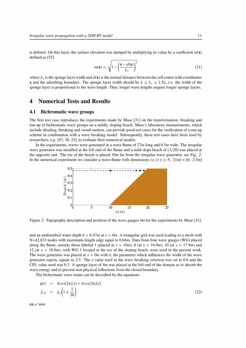
In the experiments, waves were generated in a wave flume of 27m long and 0.5m wide. The irregularwave generator was installed at the left end of the flume and a mild slope beach of (1/20) was placed atthe opposite end. The toe of the beach is placed 10m far from the irregular wave generator, see Fig. 2.In the numerical experiment we consider a wave-flume with dimensions (x, y) ∈ [−5, 21m] × [0, 2.5m]

Figure 2: Topography description and position of the wave gauges (•) for the experiments by Mase [31].

and an undisturbed water depth h = 0.47m at x = 0m. A triangular grid was used leading to a mesh withN=42,833 nodes with maximum length edge equal to 0.04m. Data from four wave gauges (WG) placedalong the flume, namely those labeled 1 (placed at x = 10m), 8 (at x = 16.9m), 10 (at x = 17.9m) and12 (at x = 18.9m), with WG 1 located at the toe of the sloping beach, were used in the present work.The wave generator was placed at x = 0m with δ, the parameter which influences the width of the wavegenerator region, equals to 2.5. The γ value used in the wave breaking criterion was set in 0.6 and theCFL value used was 0.3. A sponge layer of 4m was placed at the left end of the domain as to absorb thewave energy and to prevent non-physical reflections from the closed boundary.

The bichromatic wave trains can be described by the equations:

η(t) = Acos(2π f1t) + Acos(2π f2t)

f1,2 = fm

(1 ±

120

)(22)

RR n° 9008

12 Kazolea & Delis

where fm is the mean frequency and A the wave’s amplitude. In this work three different values of themean frequency have been used that is fm = 1, 0.6 and 0.3Hz and a = 0.015m which leads to a mediumenergy level. Changing the mean frequency leads to a variation of the waves characteristics. As fm isreduced the deep water wave steepness decreases and the probability that plunging breakers occur insteadof spilling breakers is higher for low mean frequencies. An explanation of that is given in [47] using thesurf similarity parameter defined by [5]. The first and the second case in this work use fm = 1Hz and0.6Hz respectively where spilling wave breaking occurs, while the third test case uses fm = 0.3Hz wherethe wave breaker is mainly of the plunging type. Bed friction was neglected in these test cases and thewet/dry εwd tolerance parameter was set equal to 10−6.

In order to produce the wave pattern, and since we use (8) we need the wave amplitude and frequencyof each wave component as to define the source function amplitude (9). The numerical wave trains aregenerated internally using linear theory and following the bichromatic wave pattern given in (22), toidentify the frequency components of the wave signal; however, as the actual experimental frequenciesand amplitudes deviated from the target ones, several trials were necessary to find the best match withthe measured waves. In [47] it is noted that in the experiments the generation of spurious harmonics wasnot compensated at the generator and that there was no active absorption of reflected waves, therefore itis difficult to reproduce the laboratory conditions exactly. After several trials we found the used meanfrequencies for each case respectively: fm = 1.03, 0.605, 0.31Hz

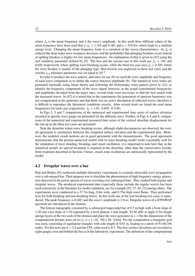
In Figs 3, 5 and 7 comparisons of the numerical and experimental time series of surface elevationrecorded at specific wave gauge are presented for the different cases. Further, in Figs 4, 6 and 8, compar-isons of the numerical and experimental measured time series of the vertical shoreline displacement forthe run-up in the three test cases are presented.

Near the shoreline where wave breaking occurs, although slight discrepancies are observed, the over-all agreement is satisfactory between the computed surface elevation and the experimental data. More-over, the modeled swash motions are in good agreement with the measurements. The good agreementdemonstrates that the present numerical model with its wave breaking model works reasonably well forthe simulation of wave shoaling, breaking, and swash oscillation. it is important to note here that, in thenumerical model, no special treatment is required at the shoreline, other than the conservative wet/dryfront treatment described in Section 3 hence, swash zone oscillations are intrinsically represented by themodel.

4.2 Irregular waves over a bar

Beji and Battjes [6] conducted multiple laboratory experiments to examine sinusoidal wave propagationover a sub-merged bar. Their purpose was to elucidate the phenomenon of high frequency energy genera-tion observed in the power spectra of waves traveling over submerged bars. They studied both regular andirregular waves. The produced experimental data (especially those include the regular waves) has beenused extensively in the literature for model validation, see for example [53, 37, 45, 21] among others. Theexperiments were conducted in a 37.7m long, 0.8m wide, and 0.75m high wave flume. They performedtests for both breaking and non-breaking waves. In this work one of the non-breaking test cases is repro-duced. The peak frequency is 0.4Hz and the wave’s amplitude is 2.9cm. Irregular waves of a JONSWAPspectrum are introduced in the domain.

The bottom topography consisted by a submerged trapezoidal bar of 0.3 m high with a front slope of1:20 and a lee slope of 1:10 separated by a level plateau 2 min length. To be able to apply 6.5m lengthsponge layers at the two ends of the domain and place the wave generator at x = 0m the dimensions of thecomputational domain were set to (x, y) ∈ [−10, 30] × [0, 0.8m]. For the computation a triangular gridwas used, consisting of equilateral triangles with side length of 0.03 m, leading to a mesh of N=40,346nodes. For this test case δ = 2.5 and the CFL value used is 0.3. The free-surface elevations are recorded ateight gauges over and behind the bar as in the laboratory experiment. The definition of the computational

Inria


Figure 3: Comparison of time series of the surface elevation in the wave gauges 8, 10 and 12 (from top tobottom)) for bicromatic waves with fm = 1Hz between numerical solution (solid line) and experimentaldata.

Figure 4: Comparison of the time series of the shoreline elevation for bicromatic wave trains producedwith fm = 1Hz between the numerical (solid line) and the experimental (dashed line) one.

domain along the centerline as well as the wave gauge locations are shown in Fig. 9.As mentioned above the wave gauges record the time series of the free surface elevation. The analysis

of the collected data carried out with the usage of the standard FFT package WAFO [50]. The datasegments, in each gauge, are 150s long. Fig. 10 shows the computed and experimental normalizedenergy spectrum for four wave gauges along the submerged bar. The numerical data slightly overestimate

RR n° 9008

14 Kazolea & Delis

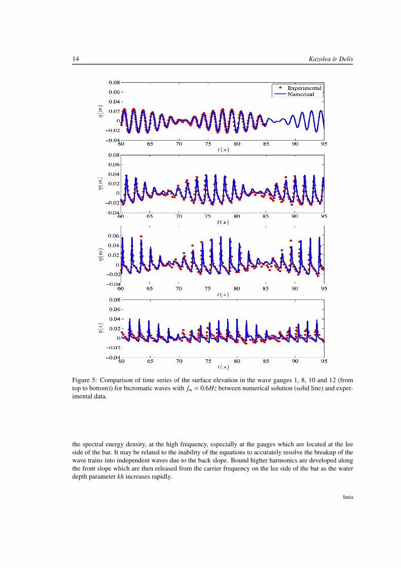
Figure 5: Comparison of time series of the surface elevation in the wave gauges 1, 8, 10 and 12 (fromtop to bottom)) for bicromatic waves with fm = 0.6Hz between numerical solution (solid line) and exper-imental data.

the spectral energy density, at the high frequency, especially at the gauges which are located at the leeside of the bar. It may be related to the inability of the equations to accurately resolve the breakup of thewave trains into independent waves due to the back slope. Bound higher harmonics are developed alongthe front slope which are then released from the carrier frequency on the lee side of the bar as the waterdepth parameter kh increases rapidly.

Inria


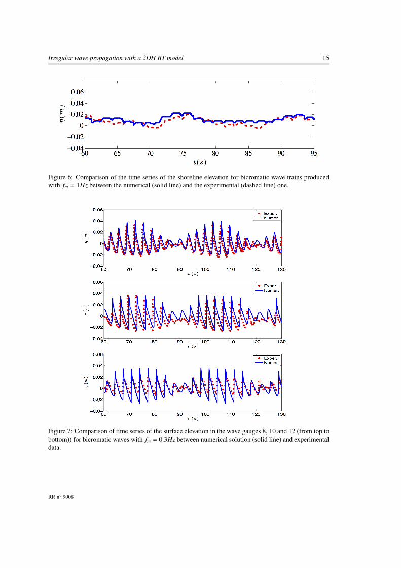
Figure 6: Comparison of the time series of the shoreline elevation for bicromatic wave trains producedwith fm = 1Hz between the numerical (solid line) and the experimental (dashed line) one.

Figure 7: Comparison of time series of the surface elevation in the wave gauges 8, 10 and 12 (from top tobottom)) for bicromatic waves with fm = 0.3Hz between numerical solution (solid line) and experimentaldata.

RR n° 9008

16 Kazolea & Delis

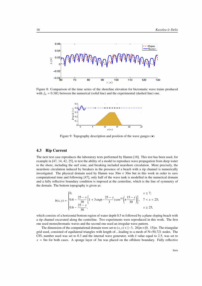
Figure 8: Comparison of the time series of the shoreline elevation for bicromatic wave trains producedwith fm = 0.3Hz between the numerical (solid line) and the experimental (dashed line) one.

Figure 9: Topography description and position of the wave gauges (•)

4.3 Rip CurrentThe next test case reproduces the laboratory tests performed by Hamm [18]. This test has been used, forexample in [47, 14, 42, 25], to test the ability of a model to reproduce wave propagation from deep waterto the shore, including the surf zone, and breaking included nearshore circulation. More precisely, thenearshore circulation induced by breakers in the presence of a beach with a rip channel is numericallyinvestigated. The physical domain used by Hamm was 30m × 30m but in this work in order to savecomputational time and following [47], only half of the wave tank is modelled in the numerical domainand a fully reflective boundary condition is imposed at the centreline, which is the line of symmetry ofthe domain. The bottom topography is given as:

b(x, y) =

0, x ≤ 7;

0.6 −25 − x

30

[1 + 3 exp(−

25 − x3

) cos10(π

15 − y30

)], 7 < x < 25;

0.6 −25 − x

30, x ≥ 25,

which consists of a horizontal bottom region of water depth 0.5 m followed by a plane sloping beach witha rip channel excavated along the centreline. Two experiments were reproduced in this work. The firstone used monochromatic waves and the second one used an irregular wave pattern.

The dimension of the computational domain were set to (x, y) ∈ [−3, 26]m× [0, 15]m. The triangulargrid used, consisted of equilateral triangles with length of....leading to a mesh of N=50,721 nodes. TheCFL number used was set to 0.3 and the internal wave generator, with δ value equal to 2.5, was set tox = 0m for both cases. A sponge layer of 3m was placed on the offshore boundary. Fully reflective

Inria


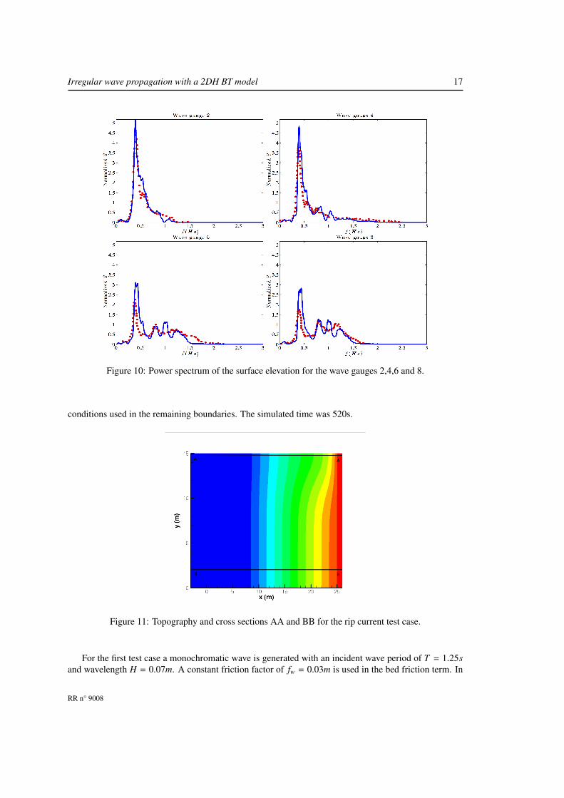
Figure 10: Power spectrum of the surface elevation for the wave gauges 2,4,6 and 8.

conditions used in the remaining boundaries. The simulated time was 520s.

Figure 11: Topography and cross sections AA and BB for the rip current test case.

For the first test case a monochromatic wave is generated with an incident wave period of T = 1.25sand wavelength H = 0.07m. A constant friction factor of fw = 0.03m is used in the bed friction term. In

RR n° 9008

18 Kazolea & Delis

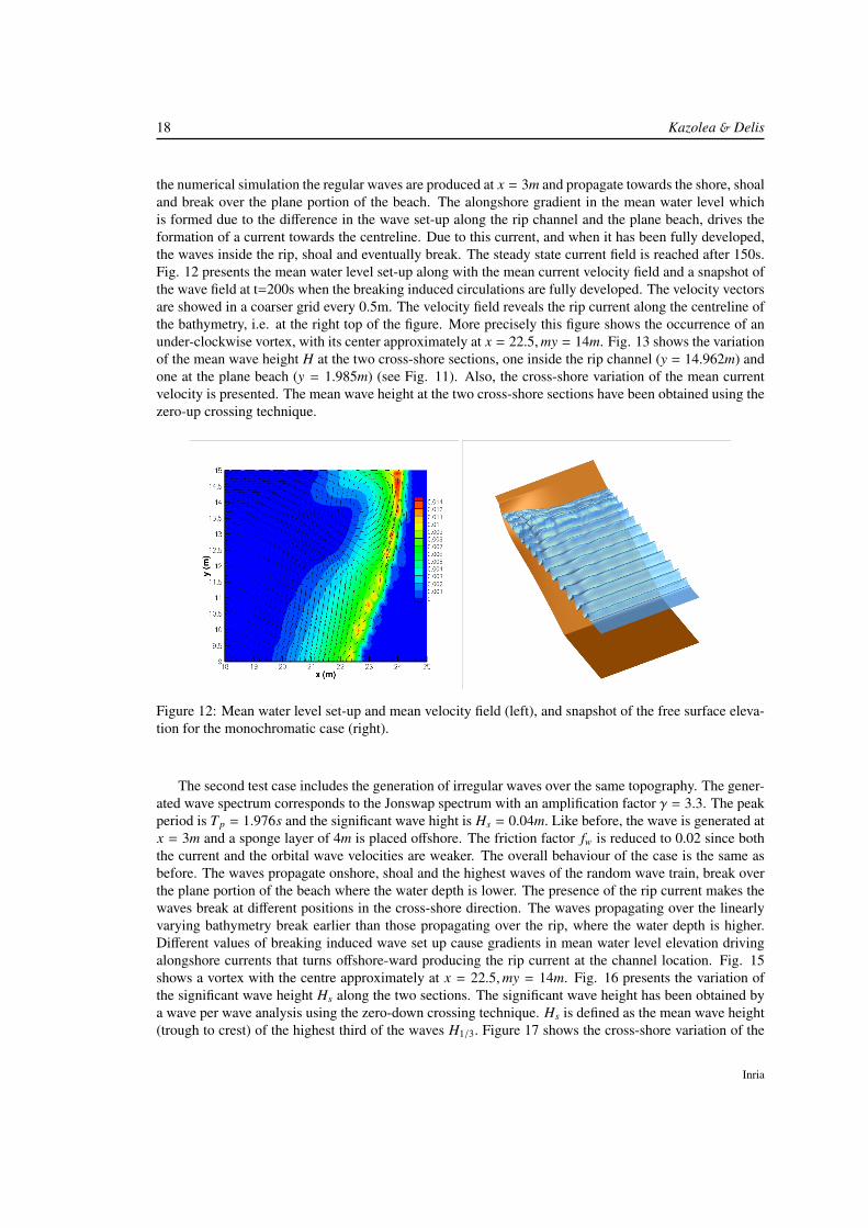
the numerical simulation the regular waves are produced at x = 3m and propagate towards the shore, shoaland break over the plane portion of the beach. The alongshore gradient in the mean water level whichis formed due to the difference in the wave set-up along the rip channel and the plane beach, drives theformation of a current towards the centreline. Due to this current, and when it has been fully developed,the waves inside the rip, shoal and eventually break. The steady state current field is reached after 150s.Fig. 12 presents the mean water level set-up along with the mean current velocity field and a snapshot ofthe wave field at t=200s when the breaking induced circulations are fully developed. The velocity vectorsare showed in a coarser grid every 0.5m. The velocity field reveals the rip current along the centreline ofthe bathymetry, i.e. at the right top of the figure. More precisely this figure shows the occurrence of anunder-clockwise vortex, with its center approximately at x = 22.5,my = 14m. Fig. 13 shows the variationof the mean wave height H at the two cross-shore sections, one inside the rip channel (y = 14.962m) andone at the plane beach (y = 1.985m) (see Fig. 11). Also, the cross-shore variation of the mean currentvelocity is presented. The mean wave height at the two cross-shore sections have been obtained using thezero-up crossing technique.

Figure 12: Mean water level set-up and mean velocity field (left), and snapshot of the free surface eleva-tion for the monochromatic case (right).

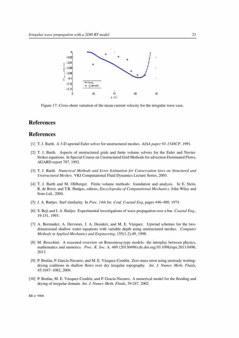
The second test case includes the generation of irregular waves over the same topography. The gener-ated wave spectrum corresponds to the Jonswap spectrum with an amplification factor γ = 3.3. The peakperiod is Tp = 1.976s and the significant wave hight is Hs = 0.04m. Like before, the wave is generated atx = 3m and a sponge layer of 4m is placed offshore. The friction factor fw is reduced to 0.02 since boththe current and the orbital wave velocities are weaker. The overall behaviour of the case is the same asbefore. The waves propagate onshore, shoal and the highest waves of the random wave train, break overthe plane portion of the beach where the water depth is lower. The presence of the rip current makes thewaves break at different positions in the cross-shore direction. The waves propagating over the linearlyvarying bathymetry break earlier than those propagating over the rip, where the water depth is higher.Different values of breaking induced wave set up cause gradients in mean water level elevation drivingalongshore currents that turns offshore-ward producing the rip current at the channel location. Fig. 15shows a vortex with the centre approximately at x = 22.5,my = 14m. Fig. 16 presents the variation ofthe significant wave height Hs along the two sections. The significant wave height has been obtained bya wave per wave analysis using the zero-down crossing technique. Hs is defined as the mean wave height(trough to crest) of the highest third of the waves H1/3. Figure 17 shows the cross-shore variation of the

Inria


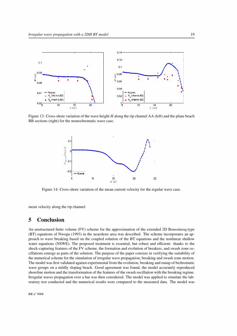
Figure 13: Cross-shore variation of the wave height H along the rip channel AA (left) and the plane beachBB sections (right) for the monochromatic wave case.

Figure 14: Cross-shore variation of the mean current velocity for the regular wave case.

mean velocity along the rip channel.

5 ConclusionAn unstructured finite volume (FV) scheme for the approximation of the extended 2D Boussinesq-type(BT) equations of Nwogu (1993) in the nearshore area was described. The scheme incorporates an ap-proach to wave breaking based on the coupled solution of the BT equations and the nonlinear shallowwater equations (NSWE). The proposed treatment is essential, but robust and efficient: thanks to theshock-capturing features of the FV scheme, the formation and evolution of breakers, and swash zone os-cillations emerge as parts of the solution. The purpose of the paper consists in verifying the suitability ofthe numerical scheme for the simulation of irregular wave propagation, breaking and swash zone motion.The model was first validated against experimental from the evolution, breaking and runup of bichromaticwave groups on a mildly sloping beach. Good agreement was found; the model accurately reproducedshoreline motion and the transformation of the features of the swash oscillation with the breaking regime.Irregular waves propagation over a bar was then considered. The model was applied to simulate the lab-oratory test conducted and the numerical results were compared to the measured data. The model was

RR n° 9008

20 Kazolea & Delis

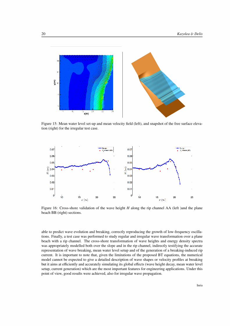
Figure 15: Mean water level set-up and mean velocity field (left), and snapshot of the free surface eleva-tion (right) for the irregular test case.

Figure 16: Cross-shore validation of the wave height H along the rip channel AA (left )and the planebeach BB (right) sections.

able to predict wave evolution and breaking, correctly reproducing the growth of low-frequency oscilla-tions. Finally, a test case was performed to study regular and irregular wave transformation over a planebeach with a rip channel. The cross-shore transformation of wave heights and energy density spectrawas appropriately modelled both over the slope and in the rip channel, indirectly testifying the accuraterepresentation of wave breaking, mean water level setup and of the generation of a breaking-induced ripcurrent. It is important to note that, given the limitations of the proposed BT equations, the numericalmodel cannot be expected to give a detailed description of wave shapes or velocity profiles at breakingbut it aims at efficiently and accurately simulating its global effects (wave height decay, mean water levelsetup, current generation) which are the most important features for engineering applications. Under thispoint of view, good results were achieved, also for irregular wave propagation.

Inria


Figure 17: Cross-shore variation of the mean current velocity for the irregular wave case.

References

References[1] T. J. Barth. A 3-D upwind Euler solver for unstructured meshes. AIAA paper 91-1548CP, 1991.

[2] T. J. Barth. Aspects of unstructured grids and finite volume solvers for the Euler and Navier-Stokes equations. In Special Course on Unstructured Grid Methods for advection Dominated Flows,AGARD report 787, 1992.

[3] T. J. Barth. Numerical Methods and Error Estimation for Conservation laws on Structured andUnstructured Meshes. VKI Computational Fluid Dynamics Lecture Series, 2003.

[4] T. J. Barth and M. Ohlberger. Finite volume methods: foundation and analysis. In E. Stein,R. de Borst, and T.R. Hudges, editors, Encyclopedia of Computational Mechanics. John Wiley andSons Ltd., 2004.

[5] J. A. Battjes. Surf similarity. In Proc. 14th Int. Conf. Coastal Eng, pages 446–480, 1974.

[6] S. Beji and J. A. Battjes. Experimental investigations of wave propagation over a bar. Coastal Eng.,19:151, 1993.

[7] A. Bermudez, A. Dervieux, J. A. Desideri, and M. E. Vázquez. Upwind schemes for the two-dimensional shallow water equations with variable depth using unstructured meshes. ComputerMethods in Applied Mechanics and Engineering, 155(1-2):49, 1998.

[8] M. Brocchini. A reasoned overview on Boussinesq-type models: the interplay between physics,mathematics and numerics. Proc. R. Soc. A, 469 (20130496):dx.doi.org/10.1098/rspa.2013.0496,2013.

[9] P. Brufau, P. García-Navarro, and M. E. Vázquez-Cendón. Zero mass error using unsteady wetting-drying coditions in shallow flows over dry irregular topography. Int. J. Numer. Meth. Fluids,45:1047–1082, 2004.

[10] P. Brufau, M. E. Vázquez-Cendón, and P. Gracía-Navarro. A numerical model for the flooding anddrying of irregular domain. Int. J. Numer. Meth. Fluids, 39:247, 2002.

RR n° 9008

22 Kazolea & Delis

[11] M. J. Castro, A. M. Ferreiro, J. A. García-Rodriguez, J. M. González-Vida, J. Macías, C. Parés, andM. E. Vázquez-Cendón. The numerical treatment of wet/dry fronts in shallow flows: Applicationto one-layer and two-layer systems. Mathematical and Computer Modelling, 42:419–439, 2005.

[12] A. I. Delis, M. Kazolea, and N. A. Kampanis. A robust high resolution finite volume scheme for thesimulation of long waves over complex domain. Int. J. Numer. Meth. Fluids, 56:419–452, 2008.

[13] A. I. Delis, I. K. Nikolos, and M. Kazolea. Performance and comparison of cell-centered and node-centered unstructured finite volume discretizations for shallow water free surface flows. Archives ofComputational Methods in Engineering, 18:57–118, 2011.

[14] Gallerano F., G. Cannata, and Villani M. An integral contravariant formulation of the fully non-linear boussinesq equations. Coast. Eng., 83:119–136, 2014.

[15] A.G. Filippini, M. Kazolea, and M. Ricchiuto. A flexible genuinely nonlinear approach for nonlinearwave propagation, breaking and run-up. Journal of Computational Physics, 310:381–417, 2016.

[16] A. George and J. W. H Liu. Computer solution of Large Sparce Positive Definite Systems. PrenticeHall: Englewood Cliffs, N.J., 1981.

[17] E. Godlewski and P. A. Raviart. Hyperbolic systems of conservation laws, Applied MathematicalSciences, vol. 118. Springer, Berlin, 1995.

[18] L. Hamm. Directional nearshore wave propagation over a rip channel: an experiment. In Proc. 23rdInt. Conf. Coastal Eng., 1992.

[19] G. Hanbin, L. Yanbao, L. Shaowu, and Luwen Q. Applications of a boussinesq wave model. InInternational Conference on Estuariew and Coasts, 2003.

[20] M. E. Hubbard and P. García-Navarro. Flux difference splitting and the balancing of source termsand flux gradients. J. Comp. Phys., 165:89–125, 2000.

[21] M. Kazolea, A. I. Delis, I. A Nikolos, and C. E. Synolakis. An unstructured finite volume numericalscheme for extended 2D Boussinesq-type equations. Coast. Eng., 69:42–66, 2012.

[22] M. Kazolea, A. I. Delis, and C. E. Synolakis. Numerical treatment of wave breaking on unstructuredfinite volume approximations for extended Boussinesq-type equations. J.Comput.Phys., 271:281–305, 2014.

[23] A. B. Kennedy, J .T. Chen, Q. Kirby, and R. A. Dalrymple. Boussinesq modeling of wave trans-formation, breaking and runup. Part I: 1D. J. Waterw., Port, Coast., Ocean Engrg., 126:39–47,2000.

[24] J.T. Kirby. Boussinesq models and their application to coastal processes across a wide range ofscales. Journal of Waterway, Port, Coastal and Ocean Engineering, 142(6), 2016.

[25] G.T. Klonaris, C.D. Memos, and N.K. DrÃ¸nen. High-order boussinesq-type model for integratednearshore dynamics. Journal of Waterway, Port, Coastal and Ocean Engineering, 142(6), 2016.

[26] Q. Liang and A. G. L. Borthwick. Adaptive quadtree simulation of shallow flows with wet/dry frontover complex topography. Comput. Fluids, 38:221–234, 2009.

[27] M. S. Longet-Higgins, D. E. Cartwright, and N. D Smith. Observation of the directional spectrumof sea waves using the motions of a floating buoy. In Proc. Conf. of Ocean Wave Spectra, 1961.

Inria


[28] P. J. Lynett. Nearshore Wave Modeling with High-Order Boussinesq-Type Equations. Journal ofWaterway, Port, Coastal, and Ocean Engineering, 132:348–357, 2006.

[29] P. A. Madsen and O. R. Sørensen. A new form of the Boussinesq equations with improved lineardispersion characteristics. Part 2: A slowing varying bathymetry. Coast. Eng., 18:183–204, 1992.

[30] P.A. Madsen, O. R. Sørensen, and H. A. Schäffer. Surf zone dynamics simulated by a Boussinesq-type model: Part II. Surf beat and swash oscillations for wave groups and irregular waves. Coast.Eng., 32:289–319, 1997b.

[31] H. Mase. Frequency down-shift of swash oscillations compared to incident waves. J. HydraulicRes, 33:3:397–411, 1995.

[32] I. K. Nikolos and A. I. Delis. An unstructured node-centered finite volume scheme for shallowwater flows with wet/dry fronts over complex topography. Comput. Methods Appl. Mech. Engrg,198:3723–3750, 2009.

[33] O. Nwogu. An alternative form of the Boussinesq equations for nearshore wave propagation. Jour-nal of Waterway, Port, Coastal, and Ocean Engineering, 119:618–638, 1994.

[34] D. H. Peregrine. Long waves on a beach. J. Fluid Mech., 27:815–882, 1967.

[35] M. Ricchiuto and A. Bollermann. Stabilized residual distribution for shallow water simulations.J.Comput.Phys, 228:1071–1115, 2009.

[36] P. L. Roe. Approximate Riemann solvers, parameter vectors, and difference schemes. J. Comp.Phys., 43:357–372, 1981.

[37] V. Roeber, K. F. Cheung, and M. H. Kobayashi. Shock-capturing Boussinesq-type model fornearshore wave processes. Coast. Eng., 57:407–423, 2010.

[38] Y. Saad. Iterative Methods for Sparse Linear Systems. PWS, 1996.

[39] H. A. Schäffer, P.A. Madsen, and R. Deigaard. A Boussinesq model for waves breaking in shallowwater. Coast. Eng., 20:185–202, 1993.

[40] T. M. Smith, M. F. Barone, and R. B. Bond. Comparison of reconstruction techniques for un-structured mesh vertex centered finite volume schemes. 18th AIAA Computational Fluid DynamicsConference, pages 1–22, 2007.

[41] O. R. Sørensen, H. A. Schäffer, and P. A. Madsen. Surf zone dynamics simulated by a Boussinesqtype model: Part III. Wave-induced horizontal nearshore circulations. Coastal. Eng., 33:155–176,1998.

[42] O. R. Sørensen, H.A. Shäffer, and L.S. Sørensen. Boussinesq-type modelling using an unstructuredfinite element technique. Coastal Eng., 50:182, 2004.

[43] R. J. Spiteri and S. J. Ruuth. A new class of optimal high-order strong-stability-preserving timediscretization methods. SIAM J. Numer. Anal., 40:469, 2002.

[44] M. Tissier, P. Bonneton, F. Marche, F. Chazel, and D. Lannes. A new approach to handle wavebreaking in fully non-linear Boussinesq models. Coastal Engineering, 67:54–66, 2012.

[45] M. Tonelli and M. Petti. Hybrid finite-volume finite-difference scheme for 2DH improved Boussi-nesq equations. Coast. Eng., 56:609–620, 2009.

RR n° 9008

24 Kazolea & Delis

[46] M. Tonelli and M. Petti. Finite volume scheme for the solution of 2D extended Boussinesq equationsin the surf zone. Ocean. Eng., 37:567–582, 2010.

[47] M. Tonelli and M. Petti. Shock-capaturing Boussinesq model for irregular wave propagation.Coastal Engineering, 61:8–19, 2012.

[48] G. D. Van Albada, B. Van Leer, and W. W. Roberts. A comparative study of computational methodsin cosmic gas dynamics. Astron. Astrophysics, 108:46–84, 1982.

[49] B. van Leer. Towards the ultimate conservative difference scheme V. A second order sequel toGodunov’s method. J. Comp. Phys., 32:101, 1979.

[50] WAFO-group. WAFO - A Matlab Toolbox for Analysis of Random Waves and Loads - A Tutorial.Math. Stat., Center for Math. Sci., Lund Univ., Lund, Sweden, 2000.

[51] G. Wei, J. T. Kirby, and A. Sinha. Generation of waves in Boussinesq models using a source functionapproach. Coastal Eng., 36:271, 1999.

[52] T.-R. Wu. A numerical study of three dimensional breaking waves and turbulence effects. PhDthesis, Cornell University, 2004.

[53] Y. Yamazaki, Z. Kowalik, and K. F. Cheung. Depth-integrated, non-hydrostatic model for wavebreaking and run-up. Int. J. Numer. Meth. Fluids, 61:473, 2009.

Inria

RESEARCH CENTREBORDEAUX – SUD-OUEST

200 avenue de la Vieille Tour33405 Talence Cedex

PublisherInriaDomaine de Voluceau - RocquencourtBP 105 - 78153 Le Chesnay Cedexinria.fr

ISSN 0249-6399

Documents

Irregular wave propagation with a 2DH Boussinesq-type