Embed Size (px)
Citation preview
Introduction Thermal Counterflow Model Results and Conclusions
SUPERFLUID VORTICES IN A WALL-BOUNDED FLOW
L. Galantucci, M. Quadrio, P. Luchini
Dip. Ingegneria Aerospaziale, Politecnico di MilanoDip. Meccanica, Università di Salerno
Ancona, 17 settembre 2009

Introduction Thermal Counterflow Model Results and Conclusions
STRUTTURA DELLA PRESENTAZIONE
1 INTRODUCTION
2 THERMAL COUNTERFLOW
3 MODEL
4 RESULTS AND CONCLUSIONS

Introduction Thermal Counterflow Model Results and Conclusions
HE4 CHARACTERISTICS
HE PECULIARITIES
permanent liquid
distinct liquid phases
λ-phase-transition
HE I: ORDINARY FLUID
ρ = 0.137 g/cm3
ν= 2.56 · 10−8m2/s
HE II: QUANTUM FLUID
very low temperatures
indistinguishable particles
Bose-Einstein quantum statistics

Introduction Thermal Counterflow Model Results and Conclusions
Two-fluid MODEL
Tisza (1940) , Landau (1941-1947)
NORMAL
ρn
vn
sn
νn
SUPERFLUID
ρs
vs
ss = 0
νs = 0
ρ = ρn +ρs
j = ρnvn +ρsvs
∂vn∂t = N .S. (vn) ∇×vs = 0
INCOMPLETE
Introduction Thermal Counterflow Model Results and Conclusions
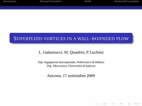
SUPERFLUID QUANTIZED VORTEX-LINES
REGIONS OF CONCENTRATED SUPERFLUID VORTICITY
very small regionscirculation of vs quantized Γ= n
h
m, n ∈N
London (1954), Landau & Lifshitz (1955): vortex-sheetsOnsager (1949), Feynman (1955): vortex-lines
HALL & VINEN, 1956
studies on uniformly rotating He II
thermodynamical discussion
experimental study
⇓QUANTIZED VORTEX-LINES

Introduction Thermal Counterflow Model Results and Conclusions
MUTUAL FRICTION FORCEHALL & VINEN, 1956
vortex lines = scattering centres⇓
momentum transfercollision rotons, phonons – vortex lines
⇓MUTUAL FRICTION FORCE
THEORY OF MUTUAL FRICTION IN UNIFORMLY ROTATING HE II
f D =−αρsΓωs ×[ωs ×
(vn −vs
)]−α′ρsΓωs ×(vn −vs
)α=α(T) , α′ =α′(T)
ωs // axis of rotation
vn and vs: average over `À `0

Introduction Thermal Counterflow Model Results and Conclusions
MUTUAL FRICTIONSCHWARZ, 1978
generic He II system
vortex – tangle
ωs = 0
THEORETICAL FORMULATION
vn and vs local
vortex curvatureself induction
vi(s) = Γ
4π
∫L
(z− s)×dz
|z− s|3
f D =−αρsΓs′× [s′× (vn −vs −vi)
]−α′ρsΓs′× (vn −vs −vi)
vL = vs +vi +αs′× (vn −vs −vi)−α′s′× [s′× (vn −vs −vi)
]

Introduction Thermal Counterflow Model Results and Conclusions
NUMERICAL SIMULATIONS
SCHWARZ, 1988
prescribed vn and vs
vi computed with LIA
analysis of vortex topology
preliminary study of reconnections
AARTS, DE WAELE, SAMUELS, BARENGHI (1994–1997)
kinematic simulations
vn prescribeduniformPoiseuilleABC model flows
vn and vs coupling

Introduction Thermal Counterflow Model Results and Conclusions
NUMERICAL SIMULATIONS
BARENGHI, SAMUELS (2001) , IDOWU et al. (2001)
self-consistent algorithm
Lagrangian description vL
vortex filament methodLocal Induced Approximation for vi
Navier–Stokes Eulerian equations vn∂vn
∂t+ (vn ·∇)vn=− 1
ρ∇p− ρs
ρns∇T +νn∇2vn − 1
ρnF ns
local F ns
BUT
all past simulations performed in unbounded domains
IMPORTANCE OF SOLID BOUNDARIES
Vortex–lines nucleation
Vortex–lines dynamics
Introduction Thermal Counterflow Model Results and Conclusions
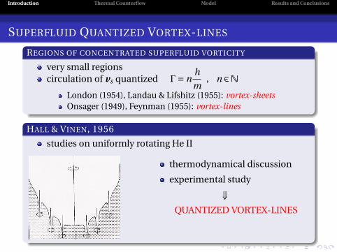
THERMAL COUNTERFLOW
IMPORTANCE
unique phenomenon
two-fluid model
fundamentals ofvortex–line dynamics
Q ⇒ q = ρsTvn
two-fluid model equations
ρn∂vn
∂t+ρn (vn ·∇)vn = ηn∇2vn − ρn
ρ∇p−ρss∇T
ρs∂vs
∂t+ρs (vs ·∇)vs = ρs
ρ∇p+ρss∇T
Introduction Thermal Counterflow Model Results and Conclusions
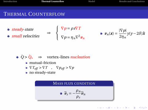
THERMAL COUNTERFLOW
steady-state
small velocities⇒
∇p = ρs∇T
∇p = ηn∇2vn
vn(x) = |∇p|2ηn
y(y−2δ)x
Q > Q∗ ⇒ vortex–lines nucleationmutual–friction∇Teff >∇T , ∇peff >∇pno steady–state
MASS FLUX CONDITION
vs =−ρn
ρsvn

Introduction Thermal Counterflow Model Results and Conclusions
COMPUTATIONAL METHOD
thermal–channel–counterflow
bidimensional domain
solid boundaries︸ ︷︷ ︸N vortex–points dynamics
vL(xk,yk, t) =[(
1−α′)(vexts +vx
s,i
)−α′vn(y)±αvy
s,i
]x+
+[(
1−α′)vys,i ∓α
(vn(y)+vext
s +vxs,i
)]y
vs,i(x, t) : superfluid induced velocity
vn(x) =−vn(y)x , vn(y) ≥ 0 , parabolic profile
vexts = vext
s x =−ρn
ρsvn : uniform superfluid velocity

Introduction Thermal Counterflow Model Results and Conclusions
COMPUTATIONAL METHOD
irrotational
incompressible
}⇒ complex-potentials
VORTEX IN A PLANE CHANNEL
conformal mapping
images method
vj(z) = vxj − ivy
j =∓iħm
π
4δ
{coth
[ π4δ
(z−zj
)]−coth[ π
4δ
(z−zj
)]}vs,i(zk) = vx
s,i − ivys,i =
∑j 6=k
vj(zk)± iħm
π
4δcoth
[ π4δ
(zk −zk
)]VORTEX–POINTS NUCLEATION
N constant
y∗ = 2
πarctan
(π
4
1
vexts
)

Introduction Thermal Counterflow Model Results and Conclusions
NUMERICAL RESULTS
T(◦K ) 1.5ρn/ρs 0.143α 0.078α′ 6.25×10⁻³
∆ptot(Pa) 10Lx(m) 0.1ηn(Pa·s) 3×10⁻⁷
δ(m) 3×10⁻⁵
vn = 0.10m/s
vexts = 0.014m/s
vortex–points sign–separation
vyL =
(1−α′)vy
s,i∓∓α
(vn(y)+vext
s +vxs,i
)+ vortices ↓− vortices ↑
y∗ ∼ δvortex nucleation on centerline

Introduction Thermal Counterflow Model Results and Conclusions
NUMERICAL RESULTSSURFACE PLOTS OF vx
s,i
t1
t3
t5
t2
t4
t6
Introduction Thermal Counterflow Model Results and Conclusions
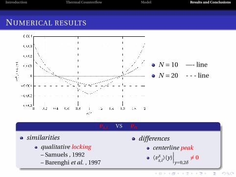
NUMERICAL RESULTS
N = 10 —- line
N = 20 - - - line
vs,i VS vn
similaritiesqualitative locking– Samuels , 1992– Barenghi et al. , 1997
differencescenterline peak
⟨vxs,i⟩(y)
∣∣∣y=0,2δ
6= 0

Introduction Thermal Counterflow Model Results and Conclusions
SUMMARY AND FUTURE WORK
SUMMARY
bidimensional numerical simulation ofHe II thermal–channel–counterflow
first simulation in wall bounded geometry
focus on:vortex–points dynamicsvortex–points nucleationsuperfluid induced velocity profile⟨vx
s,i⟩(y) vs vn(y)
FUTURE WORKS
compute vs,i mass–flux
implement vortex–points feedback on normal fluid
verify numerically flattening of normal fluid profile