KULIN/DUDININ CATCHMENTS WATER MANAGEMENT PLAN Appendix C

KULIN/DUDININ CATCHMENTS WATER MANAGEMENT PLAN Appendix C Management Options Evaluation Final Report

Kulin/Dudinin Catchments Water Management Plan Appendix C – Management Options Evaluation Final Report May 2009

PO Box 3596

Australia Fair,

QLD 4215

Australia

Tel: +61 7 5564 0916

Fax: +61 7 5564 0946

e-mail: [email protected]

Web: www.dhigroup.com.au

Client

Western Australia Department of Water

Client’s representative

Mr Jason Lette

Project Kulin/Dudinin Catchment Water Management Plan

Project No

50575

Authors

Graeme Cox (GJC)

Tony Chiffings (TWC)

Ashley Prout

Date 02 March 2009

Approved by

4 Draft GJC TWC TWC 19/04/09

3 Final Report

2 Draft Report

1 Interim Report

Rev Description By Checked Approved Date

Key words

Salinity Management plan MIKE SHE

Classification

Open

Internal

Proprietary

Distribution No of copies

Western Australia department of Water Mr Jason Lette Office Copy

1 1

© DHI Water and Environment Pty Ltd 2009

The information contained in this document produced DHI Water and Environment Pty Ltd is solely for the use of the

Client identified on the cover sheet for the purpose for which it has been prepared and DHI Water and Environment Pty

Ltd undertakes no duty to or accepts any responsibility to any third party who may rely upon this document.

All rights reserved. No section or element of this document may be removed from this document, reproduced,

electronically stored or transmitted in any form without the written permission of DHI Water and Environment Pty Ltd.

All hard copies of this document are “UNCONTROLLED DOCUMENTS”. The “CONTROLLED” document is held in

electronic form by DHI Water and Environment Pty Ltd.

iii DHI Water & Environment

CONTENTS

1 INTRODUCTION ........................................................................................................... 1

2 MANAGEMENT OPTIONS ........................................................................................... 2 2.1 Engineering ..................................................................................................... 2 2.2 Modified Farming Practice ............................................................................... 2 2.3 Vegetation ....................................................................................................... 2

3 NUMERICAL MODELLING ........................................................................................... 3 3.1 Model Setup .................................................................................................... 3 3.2 Model Calibration ........................................................................................... 10 3.3 Base Case Results ........................................................................................ 12

3.3.1 Salt Concentration and Loads ............................................................ 27

3.4 Scenarios ...................................................................................................... 30 3.5 Fine Scale Modelling ..................................................................................... 32

3.5.1 Detention Basin .................................................................................. 37

3.6 Discussion ..................................................................................................... 38 3.6.1 Effectiveness of saltbush at lowering the water table.......................... 38

3.6.2 Deep Drain Discharges ...................................................................... 39

3.6.3 LASCAM Results ............................................................................... 40

3.7 Recommendations From Model Outcomes .................................................... 41

4 FINAL OPTIONS EVALUATION ................................................................................. 42 4.1 Effectiveness At Protecting Agricultural Production ....................................... 42 4.2 Cost ............................................................................................................... 43 4.3 Environmental Impacts .................................................................................. 44 4.4 Social Impacts ............................................................................................... 44 4.5 Operational & Governance Requirements ..................................................... 45

5 CONCLUSIONS .......................................................................................................... 46

6 REFERENCES ........................................................................................................... 47

FIGURES

Figure 1 Model extents and topographic grid. ............................................................................. 5 Figure 2 Daily rainfall used as input to the model. ....................................................................... 5 Figure 3 Daily potential evaporation used as inputs to the model. ............................................... 6 Figure 4 - Vegetation codes map (from Table 1) ......................................................................... 7 Figure 5 – Applied rooting depth pattern for crop, crop, bare fallow, crop, crop, pasture as model

input for generating soil water balance (Pattern was repeated as per Table 1). .......... 7 Figure 6 - Areas of the catchment (green) where detention storage was applied to represent

imperfect surface drainage. ......................................................................................... 8 Figure 7 - Soil types map (Codes in Table 2) ............................................................................ 10

iv DHI Water & Environment

Figure 8 – Initial (1950) depth to groundwater. .......................................................................... 11 Figure 9 – Simulated and observed ground water levels, (X axis is the date and Y axis depth

below ground (m)). .................................................................................................... 12 Figure 10 – Simulated and observed ground water levels, (X axis is the date and Y axis depth






below ground (m)). .................................................................................................... 18 Figure 16 – Simulated catchment water balance from 1/1/1950 to 1/1/2008. ............................ 19 Figure 17 – Annual flow duration curve from MIKE SHE and other sources for comparison...... 19 Figure 18 – Mean annual recharge (UZ to SZ) from 1975 to 2008 (mm/yr). .............................. 20 Figure 19 – Groundwater recharge for different vegetation based on field leakage studies

throughout Australia (CSIRO). .................................................................................. 21 Figure 20 – Simulated depth to groundwater for December 2007. ............................................ 22 Figure 21 – Simulated area with water table within 1m. ............................................................ 23 Figure 22 – Simulated depth to groundwater for December 2029. ............................................ 24 Figure 23 – Simulated areas with water table within 1m for 2008 and 2030. ............................. 25 Figure 24 – Simulated Groundwater Cross Section A-B. ........................................................... 26 Figure 25 – Simulated Groundwater Long Section C-D (Dec 2029). ......................................... 26 Figure 26 – Typical simulation of overland flow during the January 2006 flood event................ 27 Figure 27 – Modelled runoff and salinity at the catchment outlet for the Base Case and Base

Case with 20% less rainfall. ...................................................................................... 29 Figure 28 – Modelled salt load at the catchment outlet for the Base Case. ............................... 29 Figure 29 – Drains implemented in MIKE SHE as SZ drainage at 2m below the ground in the

blue cells (Farmer mapped salinity is white hatch). ................................................... 33 Figure 30 – Calibrated deep drain flow. .................................................................................... 34 Figure 31 – Modelled salt load at the catchment outlet for Scenario 8 – Based Case (Fine Scale

model). ...................................................................................................................... 36 Figure 32 – Modelled salt load at the catchment outlet for Scenario 9 – Single deep drain linking

existing drains. .......................................................................................................... 36 Figure 33 – Modelled salt load at the Kulin\Dudinin Catchment outlet for Scenario 11 –

Combination. ............................................................................................................. 37 Figure 34 – Simulated inflow and outflow to the proposed 2ha detention basin......................... 38 Figure 35 – Simulated inflow and outflow to the proposed 6ha detention basin......................... 38

TABLES

Table 1 – Vegetation Rotations ................................................................................................... 6 Table 2 - Unsaturated zone soil type properties .......................................................................... 9 Table 3 - Saturated zone parameters ........................................................................................ 10 Table 4 - Simulated areas with shallow water table. .................................................................. 21 Table 5 – Scenarios simulated with the course resolution model. ............................................. 30 Table 6 – Summary of results from the course resolution modelling. ........................................ 31 Table 7 - Saturated zone Hydraulic Conductivity for fine scale model ....................................... 32 Table 8 – Scenarios simulated with the fine scale model. ......................................................... 34

v DHI Water & Environment

Table 9 - Summary of results from the fine resolution modelling. .............................................. 35 Table 10 – Summary statistics from LASCAM model. ............................................................... 40 Table 11 – Summary of model observations and resultant recommended management

strategies. ............................................................................................................... 41 Table 12 – Estimated Cost for Option B – Engineering. ............................................................ 43 Table 13 – Estimated Cost for Option C – Vegetation. .............................................................. 44

1 DHI Water & Environment

1 INTRODUCTION

This appendix details step two of the management plan development. The plan seeks to

provide a best practice mix of management options, as appropriate to achieve effective

and acceptable salinity management for the catchment. This encompasses at least

consideration of the following:

Engineering (eg banks, diversions, drains, groundwater pumping, pipes,

catchment storage);

Modified farming practice (e.g. use of perennials and alternative cropping

systems); and

Revegetation (eg Oil Mallees) and Remnant vegetation (protected, enhanced).

The landholder consultation produced a number of management options that the

community was interested in pursuing. A numerical model was then developed to

determine the effectiveness of the proposed options at controlling groundwater levels

and the impact on surface water quantity and quality. The most effective and feasible

options were then refined and evaluated in terms of effectiveness at protecting

agricultural production, costs, and operational requirements (e.g. governance and

maintenance).


2 MANAGEMENT OPTIONS

Based on public consultation and committee input, interest was shown in the following

options for managing salinity in the catchment:

2.1 Engineering

These options help to prevent water from recharging and remove saline groundwater:

Surface water management: Incorporating surface water drains into farm and

catchment water to reduce opportunity for ponding and subsequent groundwater

recharge.

Deep drains: Using deep drains to lower watertables, preventing continued

accumulation of salts while allowing rainfall to leach salt from the upper soil

profile. This technique increases the rate of discharge, and consequently reduces

the area of groundwater discharge necessary to establish equilibrium.

Evaporation basins can be used to dispose of saline groundwater, or if suitable

conditions exist, water can be discharged to natural drainage lines.

2.2 Modified Farming Practice

To modify current agronomic practices with alternative, economically viable systems,

that increase evapotranspiration and reduce the amount of water percolating below the

root zone:

Alternative cropping systems: Crops and crop rotations that promote higher

water use e.g. continuous cropping verse pastures in a rotation.

Use of perennial plants: Deep rooted pastures which are capable of growing

throughout the year, and trees or fodder shrubs, which combine the advantages

of deep root systems and year round growth with higher water use, due to their

large leaf area.

2.3 Vegetation

Saltland pastures and crops: Saltland plants can provide some production from what is

otherwise generally unusable land.

Revegetate areas that maybe significant sources of recharge but offer low crop

potential. eg deep sands.

Revegetate areas at immediate risk of salinity (watertables 2-5 m and rising

trends) with perennials systems, continuos crops and trees (such as oil mallees).

Protect, manage and enhance the remnant vegetation: To maintain existing water

use and contribute to reducing groundwater recharge.


3 NUMERICAL MODELLING

The MIKE SHE modelling system was used to simulate the effectiveness of the

management options. It was selected for its ability to simulate realistic linkages between

surface water and groundwater, as well as dynamic distributed infiltration through the

unsaturated zone and vegetation-based soil-water deficits. In this context, MIKE SHE is

widely recognised as more reliable and defensible for decision-making. MIKE SHE is

regularly and independently reviewed as the most comprehensive and advanced model

for integrated catchment modelling (US Army Corp of Engineers et. al, 2002; Kaiser

Hill Company, 2001; Camp, Dresser and McKee, 2001; Aqua Terra et. al, 2001). Full

details of the MIKE SHE theory are given in the MIKE SHE User Manual (DHI, 2008).

3.1 Model Setup

The model domain covered the Dudinin Catchment and extended slightly into the

Lockhart River as shown in Figure 1. The horizontal model resolution was 200m. The

model topography was sampled from a 10m DEM provided by Department of

Agriculture and Food (DAFWA). Minor closed depressions in the model topographic

grid, which are generally an artefact of the DEM interpolation, were filled.

Historical daily rainfall and reference evaporation data was obtained from SILO data

drill (www.nrm.qld.gov.au/silo). To simulate future conditions the data from 1988 to

2008 was repeated into the future.

The land use\vegetation changes across the catchment were represented by different

rooting depths. Figure 4 shows spatial variation of vegetation and Table 1 shows the

corresponding vegetation rotations. The rooting depth was varied on a monthly basis

based on the following formulae:

Applied Rooting Depth = Crop Coefficient x Max rooting Depth x Calibration

Factor

Crop coefficients were obtained from AgET (Argent and George, 1997). The calibration

factor was used to tune the recharge amounts during calibration. Figure 5 shows the

calibrated rooting depth pattern for all vegetation excluding trees which were a constant

5000 mm.

http://www.nrm.qld.gov.au/silo



Figure 1 Model extents and topographic grid.

Figure 2 Daily rainfall used as input to the model.


Figure 3 Daily potential evaporation used as inputs to the model.

Table 1 – Vegetation Rotations

Code Vegetation Rotation

1 Trees Constant Trees

2

Crop/pasture/fallow

post1950 1950 - 1965 Crop, Crop, Bare Fallow, Crop, Crop, Pasture

post1965 Crop, Crop, Pasture

3 Crop/pasture post1965 1950 - 1965 Trees

post1965 Crop, Crop, Pasture

4 Saltland post2007 post1950 Crop, Crop, Pasture

post2007 Bare Soil


Figure 4 - Vegetation codes map (from Table 1)

Figure 5 – Applied rooting depth pattern for crop, crop, bare fallow, crop, crop, pasture as model input

for generating soil water balance (Pattern was repeated as per Table 1).

Advice from the landowners on the committee was that for the period 1950 – 1965 most

farmers would apply a Crop/Pasture/Fallow cycle. Since 1965 approximately 2/3 of

farmers would have applied a 50/50 cropping/pasture cycle and the rest would have

continually cropped. This equates to an average of 75% cropping/25% pasture. This is

in line with the assumptions in the modellings which assume 67% cropping/33%

pasture post 1965.

Note, the extent and timing of assumed clearing is approximate. Code 3 (post 1965) in

Figure 4 was not all cleared in 1965, it was cleared over decades leading up to or around

1950 1951 1952 1953 1954 1955

[s]

0.0

0.5

1.0

[()]

Le

af A

re

a In

de

x

0

200

400

600

[millimeter]

Ro

ot D

ep

th


1965. It has also been suggested by the Committee that the Code 2 (cleared pre 1950)

could extend further up the valley. These approximations to the timing of the clearing of

the higher parts of the catchment may lead to lower confidence in the modelled water

tables in these areas. However the model has been calibrated to bore levels in this area

(Bore 14, 15 and 20) to minimise any bias and the salinity risks lie lower in the

catchment. Future modelling could be based on a better reconstructed clearing map.

The Dudinin and Kulin Creeks were explicitly represented as 1D channels (MIKE11)

with trapezoidal cross section (4-10m bed, 0.4m deep, 1:1 batters) and with the top of

bank aligned with the topographic grid. These channels were coupled to the aquifer

using a river bed only conductance with a very low leakage coefficient of 1e-20. This

leakage coefficient effectively limits significant exchange with the groundwater.

Observations note that groundwater does not directly intersect the creek beds (ie no

baseflow results), and is unlikely to during the simulation period. No overbank flooding

was allowed back out of the 1D channel (i.e. one way flow from overland flow to

channels) and kinematic routing was applied to both branches.

Figure 6 - Areas of the catchment (green) where detention storage was applied to represent

imperfect surface drainage.


Overland flow was simulated using the finite difference method with a Mannings n of

0.1. Detention storage of 30mm was applied to areas of the valley floor to simulate

imperfect surface drainage as shown in Figure 6. This accounts for subgrid scale

depressions. Any large depressions (e.g. towards the bottom of the catchment) are

explicitly represented in the topographic grid will retain water and overflow after a

runoff event.

Unsaturated zone was simulated using the 2 Layer Model. A DAFWA soils map of the

catchment was simplified to four basic soil types with the properties in Table 2. The

spatial extents of each soil type are shown in Figure 7. The soil properties were initially

estimated from the AgET soils database (Argent and George, 1997) but the final

properties where fine tuned during model calibration, particularly the saturated

hydraulic conductivity.

Table 2 - Unsaturated zone soil type properties

Soil Code 1 2 3 4

Name Valley Sandy

Duplex

Ironstone

Duplex

Salt Lakes

(m/s)


Figure 7 - Soil types map (Codes in Table 2)

The saturated zone was initially simulated in the coarser grid model (200m) using three

layers as parameterised below. The model was later altered to account for observed

permeability (from soil pits) and drain flows (50 m grid model).

Table 3 - Saturated zone parameters

Layer

Lower Level

(m below

surface)

Hydraulic Conductivity

(m/d) Specific

Yield (-) Horiz. Vert.

Sediments 3 1.04 0.10 0.1

Weathered 25* 0.05 0.05 0.1

Saprock 30 0.50 0.50 0.1 *25m except in valley floor below Kulin/Dudinin Creek confluences where 5m was used to

represent a palaeochannel in the bottom layer.

3.2 Model Calibration

There was limited data to calibrate the model. Groundwater data comprised of water

table levels measured at approximately 28 sites drilled by DAFWA and two by farmers.

The additional two sites, drilled in the 1950s for stock watering purposes, were also able

to be used as the water table at this time was recorded. The levels in 2007 measured


showed rises of 17 and 29m. These increases formed the basis to calibrating the

recharge component of the model. Approximately half of the remaining bores had data

from 2000 to 2007, while the other half had only one or two points measured in 2007.

The bore locations are shown in a figure in the main document.

The model was run from 1950 until 2007. The soil surface saturated hydraulic

conductivity was adjusted until the mean annual runoff was obtained that is similar to

measured from nearby catchments.

Rooting depth was then adjusted to get recharge/groundwater response observed in bore

records placing heavy reliance on the 1950 bores. The calibration plots are shown in the

next section.

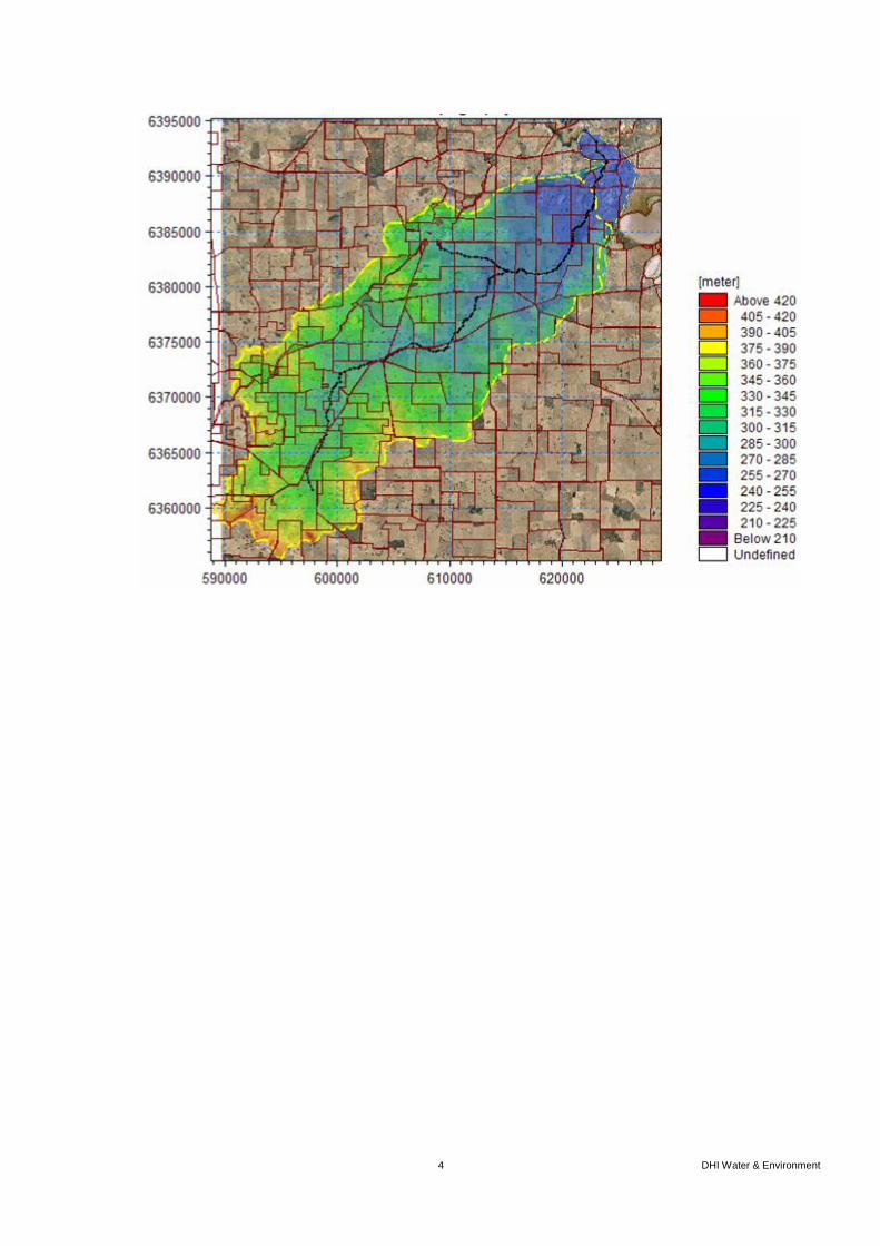
Finally, the initial (1950) water table elevation across the model domain was adjusted

until the observed bores matched as closely as possible. The adopted levels are shown in

Figure 8 and indicate that levels of 15-18m below the valley floor, and elsewhere are at

the model bedrock (30m below). Note the ‘calibrated’ levels in the lower part of the

catchment are possibly deeper than might be expected. Additional bore information in

the valley floor from the 1950s would be the only way to support this but is unavailable.

Figure 8 – Initial (1950) depth to groundwater.


3.3 Base Case Results

Figure 9 to Figure 15 show the simulated depth to groundwater at a number of bores,

along with the observed water levels. Figure 9 shows the results for the two bores

drilled in the 1950s. The simulated rise is reasonably close for both bores indicating the

simulated recharge rates are suitable.

The other bores match closely with the exception of bores in the upland areas where the

measured levels are generally more than 30m below. See bore 07KU17. This may be

partially due to the deeper regolith higher in the catchment, which is not incorporated

into the model (eg 40 to 50m not 30m as assumed). Also some upland areas were

cleared after 1965 (eg Bores 07KU16-19), where as it was assumed in the model that all

upland areas were cleared in 1965. This would result in the model over estimating the

total recharge to the groundwater in these areas and hence higher than observe

groundwater levels.

It is interesting to note the simulated rate in rise (and hence recharge) is generally the

greatest in the 1960s and has reduced somewhat since then. This is supported by

anecdotal evidence (Mike Wilson, pers. comm., 2006) that indicates this period was

wetter than average where machinery commonly got bogged. Mean monthly rainfall

residuals analysis of rainfall also supports this result.

Figure 9 – Simulated and observed ground water levels, (X axis is the date and Y axis depth below

ground (m)).



ground (m)).



ground (m)).



ground (m)).



ground (m)).



ground (m)).



ground (m)).

Figure 16 shows the catchment water balance for the period of 1950 to 2008. The

average recharge is 21.5 mm/yr and surface runoff (River + OL boundary) is 5.1 mm/yr.

The surface runoff rate of 5 mm/yr is significantly influenced by the Jan 2006 flood

event. If this event was removed the rate would drop to approximately 3.5mm/yr which

is similar to the nearby Toolibin catchment. As a result it is concluded that the figures

obtained above are suitable for use in modelling catchment behaviour.

Figure 16 also shows the approximate percentage of the largest water balance

components. The groundwater recharge of 6% is basically the root cause of the salinity

problems in the catchment. Under preclearing conditions, the groundwater recharge

component would probably be less than 0.5% and the evapotranspiration would be

closer to 99%.

Figure 17 shows how the simulated annual flow duration curve compared with other

local sources of information. MIKE SHE produces similar flows to LASCAM but

compared to the Toolibin Gauge produces significantly more low flows (50 percentile

and less). This is probably due to the fact that the Toolibin catchment has significantly

more depression storage which prevents low flows from reaching the gauge.


Figure 16 – Simulated catchment water balance from 1/1/1950 to 1/1/2008.

Figure 17 – Annual flow duration curve from MIKE SHE and other sources for comparison.

0

1

10

100

1,000

10,000

100,000

0% 20% 40% 60% 80% 100%

Proportion of Time Less Than

An

nu

al F

low

(M

L/y

r)

Dudinin Ck Modelled

(MIKE SHE 1965-2005)

Dudinin Ck Modelled

(LASCAM 1965-2005)

Toolibin Gauged (609010

scaled for area 1979-

2005)


Figure 18 shows the mean annual recharge over the period of 1950 to 2008. The highest

recharge (38-48mm/yr) is occurring in the edges of the valley floor due to the combined

effect of the assumed earlier tree clearing and the lighter soils than in the valley. The

valley floor with the heavier soil averages 26mm/yr. The areas with trees retained have

virtually no recharge. Figure 19 supports the simulated recharge.

Figure 18 – Mean annual recharge (UZ to SZ) from 1975 to 2008 (mm/yr).


Figure 19 – Groundwater recharge for different vegetation based on field leakage studies throughout

Australia (CSIRO).

Figure 20 shows the simulated depth to groundwater for December 2007 overlayed by

areas perceived by the farmers as being salt affect (white hatching). The correlation is

reasonable however the simulated area within two metres is significantly larger than the

farmer perceived areas (8100ha vs. 3400ha). Two meters is generally assumed to be the

critical depth however this is dependent on soil type and decreases with sandy soils.

There is also a time lag from when the groundwater approaches the surface and when

salinity effects can be seen, which could explain some of the difference also. Table 4

shows that 3400ha corresponds to somewhere between 0.5m and 1m to the water table.

Based on this, 1m was adopted as the critical depth to groundwater to classify an area as

salt affected in further analysis.

Table 4 - Simulated areas with shallow water table.

Depth To Water Table

2008

Area

2030

Area

ha %* ha %*

Less than 0.5m 870 2 1580 3

Less than 1m 4150 7 8000 14

Less than 2m 7990 14 12800 22

Less then 3.5m 12040 21 17200 30

Notes: * Percent of total catchment

Figure 21 shows the growth of the shallow water table area over time. The period from

2000 to 2005, shows a reduction in area reflecting a period of low rainfall years. This

result is supported by observed bore levels. The period from 1992 to 2000 was a

somewhat wetter period that saw the area grow quickly. As the rainfall and potential

evaporation from 1988-2008 were repeated in the model for estimating future changes,

a similar pattern is simulated of a quick rise from 2012 to 2018, followed by a reduction

from 2018 to 2030. Note that even though the shallow water table area may decrease

over a period, the salt affected area is unlikely to reduce as fast, if at all. This is because

the salt will accumulate in the soil profile during the period of shallow water table and


remain in the soil profile even if the water table reduces. Some downward leaching of

salt may occur in the soil profile due to rainfall, but this process is even less likely

during these corresponded lower rainfall periods. Low permeabilities also suggest

reversibility in salt accumulation is likely to be a lengthy process.

Figure 21 also shows the model outcome is quite sensitive to lower future rainfall

which could be possible under climate change.

Figure 20 – Simulated depth to groundwater for December 2007.


Figure 21 – Simulated area with water table within 1m.

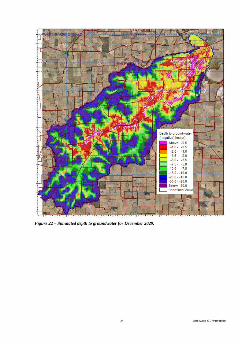
Figure 22 shows the depth groundwater in December 2029 and Table 4 shows the

corresponding areas.

0

2,000

4,000

6,000

8,000

10,000

19

50

19

55

19

60

19

65

19

70

19

75

19

80

19

85

19

90

19

95

20

00

20

05

20

10

20

15

20

20

20

25

Year

Are

a w

ith

wa

tert

ab

le w

ith

in 1

m (

ha

)

Base Case

Base Case with 20% less rain


Figure 22 – Simulated depth to groundwater for December 2029.


Figure 23 – Simulated areas with water table within 1m for 2008 and 2030.


Figure 24 – Simulated Groundwater Cross Section A-B.

.

Figure 25 – Simulated Groundwater Long Section C-D (Dec 2029).


Figure 26 – Typical simulation of overland flow during the January 2006 flood event.

Figure 26 gives an indication of how MKE SHE simulates overland flow using the Finite

Difference Method. Water flows from cell to cell depending on the surrounding water

elevations (diffusive flow equation). This allows the effect of large depressions and

increased infiltration time on flow paths to be simulated. This has been observed to be

an important phenomena affecting salinity in the catchment.

3.3.1 Salt Concentration and Loads The salt concentration in runoff from wheatbelt catchments is complex, dynamic over

time and space and often strongly related to flow. There are limited flow and salt

concentration data available from the study and nearby catchments which makes the

task of estimating the impact of the various management options difficult. To allow

basic estimates of salt concentration and total salt load to be made for the purpose of

option comparison, the salt load at the study catchment outlet was calculated. This was

based on the following estimates of salt concentrations from various runoff sources:

Good Land Runoff: 400 mg/L

This is the runoff from areas that express no signs of salinity and is the average

concentration in runoff typically measured in the Kulin Catchment from areas

with no significant signs of salinity (e.g. upstream of the existing drains in

Dudinin Ck and from the upper parts of Kulin Ck.). It is also typical of the

average concentrations found in the Toolibin catchment prior to 1980.


Salt Land Runoff: 12,500 mg/L

Dogramaci et al (2004) analysed the salinity from Lake Toolibin catchment from

the salinity record over the last 20 years and suggested that the surface water

salinity has increased from ~ 900 mg/L to ~ 1,800 mg/L for an 8% increase in

area underlain by shallow watertable. Assuming the runoff rate from this land is

the same as the rest of the catchment, this 900 mg/L increase would require an

average concentration of 11,250mg/L (900/0.08) from the salt land. Another

source of salt generation data from saline land is that of a CRC Future Farm

Industries project, at Yealering, located 50 km west of the Kulin-Dudinin

Catchment. At this site, a 25 ha bunded saline paddock (a control area for a

saltland treatment) yielded 0.37 t/ha/yr (pers. comm. George R, 2008).

Assuming an average runoff rate from the saline land is 3.2 mm/yr, this equates

to an average concentration of 11,500mg/L.

Saltland Perennial Runoff: 6,000 mg/L

This is based on preliminary results from the same CRC FFI project at

Yealering. At this site, a 25 ha bunded saline paddock with saltland perennial

vegetation is producing runoff with approximately half the salt concentration of

a control area with no treatment (pers. comm. George R, 2008). These are

preliminary results at and early stage in the project and may change over time.

This trial has also shown that the runoff volume from the saltland perennial

vegetation is approximately half that of a control area with no treatment (pers.

comm. George R, 2008). This observation has been incorporated into the load

calculations also.

Groundwater discharge: 25,000 mg/L

This is based on the average concentration measured from bores in the area and

the existing deep drains discharge measured mostly in 2006. Note, due to in-

drain and in-stream evaporation losses, it is estimated that groundwater driven

streamflow would need to consistently exceed 5 to 10 L/s before Dudinin Creek

would flow continuously to the end of the catchment. At this time, particularly

in winter, flow would reach lower into the catchment. In the mean time, the salt

load will be precipitated on the creek bed and required significant surface runoff

events to mobilise it.

Based on these concentrations and the results simulated by MIKE SHE (runoff,

flow, areas with groundwater within 1m and area planted to saltland perennials

(vegetation options), the averaged salt concentration and loads were calculated on an

annual basis at the catchment outlet. Figure 27 and Figure 28 show these results for

the Base Case (Do Nothing) Scenario.

While this method is simplistic, it does allow a simple and transparent method of

estimating the averaged salt concentration and loads with the purpose of comparing

management options.

Figure 27 shows the simulated runoff is dominated by large and infrequent flood

events. These events occur every 5 to 10 years but appear to have increased in

magnitude from 1988 to 2008. This is repeated in the forecast time period due to the

repetition of the climatic data. Figure 27 also shows the simulated stream flow


salinity started rising in 1970 and accelerated after 1991 with some periods of

reduction. This is inline with the growth of the shallow water table area over time

(Figure 21) including the reduction during dryer period. These reductions maybe an

artefact of the modelling assumption and it maybe that a ‘ratchet’ effect (up only)

actually occurs. Figure 27 also shows the simulated stream flow salinity is quite

sensitive to the future rainfall with a 20% reduction causing the simulated stream

flow salinity to plateau.

Figure 28 shows the salt load from the catchment is increasing but dominated by

large and infrequent flood events which ‘flush’ the majority of the salt through the

system. The background salt (from rainfall) that comes off the catchment naturally

is relatively consistent as expected, but the salt from the salt land becomes

prominent after 1989 and increases into the future.

Figure 27 – Modelled runoff and salinity at the catchment outlet for the Base Case and Base Case with

20% less rainfall.

Figure 28 – Modelled salt load at the catchment outlet for the Base Case.

0

1,000

2,000

3,000

19

50

19

55

19

60

19

65

19

70

19

75

19

80

19

85

19

90

19

95

20

00

20

05

20

10

20

15

20

20

20

25

Year

Str

ea

mfl

ow

Sa

lin

ity

(m

g/L

TD

S)

0

10,000

20,000

30,000

40,000

50,000

60,000

70,000

Ru

no

ff (

ML

/yr)

Runoff - Base Case

Streamflow Salinty- Base Case

Streamflow Salinty- Base Case less 20% rain

0

20,000

40,000

60,000

80,000

100,000

120,000

140,000

19

50

19

55

19

60

19

65

19

70

19

75

19

80

19

85

19

90

19

95

20

00

20

05

20

10

20

15

20

20

20

25

Year

Sa

lt L

oa

d (

t/y

r)

Groundwater Discharge Salt

Saltland Runoff Salt

Catchment Runoff Salt


3.4 Scenarios

Based on the salinity management options discussed in section 2, a number of scenarios

were defined to test in the numerical model. These are given in Table 5. Scenario 0 and

1 were discussed in the previous section. For the other scenarios, the model was run

from 2008 to 2030. The results are summarised in Table 6.

Table 5 – Scenarios simulated with the course resolution model.

Scenario

Number Scenario Description

0 Base Case (Do Nothing) as defined in sections above

1 Base Case (Do Nothing) with 20% less rainfall

2 Trees replanted on all upland areas code 2 (65% of catchment)

3 Continuous cropping on arable land i.e. no perennial pastures.

4 2m deep drains covering area within 1m at Dec 2007 (4100ha)

5 Single deep drain parallel to Dudinin Ck linking existing drains

6 Surface Water Management - No depression storage on valley floor

7 Saltland Perennial System covering area within 1m at Dec 2007 (4100ha)


Table 6 – Summary of results from the course resolution modelling.

Scen

ario

Scenario

Short

Description

Area with

water table

less than

1m in 2030

(ha)

Change in

2030 Area

Compared

to Base

Case

(ha)

(%)*

Mean

Salinity

Concentra-

tion

2025-2030

(mg/L) #

Mean

Runoff

Volume

2025-2030

(ML/yr)

Mean Salt

Load 2025-

2030

(t/yr)

0 Base Case 8,000 0 1,800 16,400 29,100

1 Base Case 20%

less rainfall

3,800

-3,200

-40% 1,200 10,100 11,600

2 Trees on all

upland areas

7,100

-900

-11% NA NA NA

3 Deep rooted

farming

5,400

-2,600

-32% NA NA NA

4 2m Deep

drains (4100ha)

4,100

-3,900

-49% 17,400 17,400 70,900

5

Single deep

drain linking

existing drains

7,500

-500

-6% 13,800 16,700 41,400

6 Surface Water

Management

7,800

-200

-2% NA NA NA

7

Saltland

Perennial

System **

2,100

-5,900

-74% ~1,700 ~15,900 ~22,200

Notes:

* Percent reduction from Base Case area is also given. In 2008, 4100ha was modelled with

water table less than 1m.

# Time weighted mean based on the mean annual concentration for each of the 5 years summed

and then divided by 5. This is significantly higher than the flow weighted mean which may be

calculated by dividing the last column by the second last column. Time weighted mean is used

because it is not affected by floods as much.

** A significant limitation of the model is the fact that there is no restriction in the water use by

vegetation and the salt concentration in the ground water. The model assumes that if the

groundwater rises into the root zone then the vegetation can extract that water. With the very

saline groundwater experienced in the study catchments it is unlikely the vegetation will be able

to use much of this water. Some proposed vegetation maybe able to use saline groundwater (eg

Salt bush and lucerne) but this will be restricted by the high groundwater salinity. This attribute

of the model will lead to a significant over estimation of the effectiveness of this scenario at

managing the catchment salinity. Local empirical data suggests that saltland plantings reduce

watertables by between 0.1 to 0.5m.


3.5 Fine Scale Modelling

Due to difficulty in modelling the existing deep drains observed flows, a finer scale

model was developed (50m grid). Overland flow simulation had to be simplified to the

lumped model in MIKE SHE as the model run times became too large. The saturated

zone hydraulic conductivities were recalibrated to those given in Table 7. These values

are supported by the test pits which generally showed low hydraulic conductivities and

are in line with published values (George 1992). However these values are significantly

lower than those adopted for the course scale model. The calibration results for the

deep drain flow are shown in Figure 30.

Table 7 - Saturated zone Hydraulic Conductivity for fine scale model

Layer Hydraulic Conductivity (m/d)

Horz. Vert.

Sediments 0.010 0.001

Weathered 0.010 0.001

Saprock 0.50 0.050

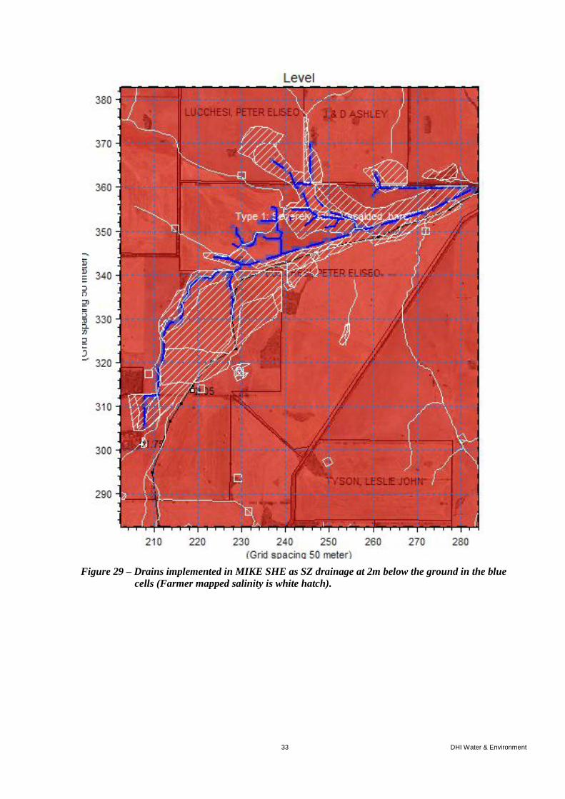
Based on the outcomes from the course-scale model, the management options were

refined to those shown in Table 8. For each scenario, the model was run from 2008 to

2030. The results are summarised in Table 9 and shown graphically in Figure 31, Figure

32 and Figure 33. These figures all show that the majority of the salt movement occurs

during the years with large flow events. The contribution from saltland is the dominant

source of salt post 2000 and grows into the future. Figure 32 shows that although the

load from the deep drains is less than 10% of the total load, it is quite consistent and

during the years with no major runoff events is the dominant source with over 90% of

the load. This would generally express itself as was experienced when the existing

drains were open; creek flow being of high salinity concentration for much longer than

previously experienced. Figure 33 shows the total load of the combination option is

approximately half of the load from the other figures and the ground water contribution

(from the deep drains) is almost non existent. This is because the vegetation is assumed

to be planted right up to the edge of the drains and thereby limiting the inflow into the

drains.


Figure 29 – Drains implemented in MIKE SHE as SZ drainage at 2m below the ground in the blue

cells (Farmer mapped salinity is white hatch).


Figure 30 – Calibrated deep drain flow.

Table 8 – Scenarios simulated with the fine scale model.

Scenario

Number Scenario Description

8 Base Case (Do Nothing)

9

Engineering Option:

Single deep drain parallel to Dudinin Ck linking existing drains and

extending to upstream of Commonwealth Road where a detention basin

will be sited.

Drain lengths: 13km existing and 13km new. Drain Depth: 2m deep.

10

Vegetation Option:

Saltland perennials (e.g. saltbush blocks and alleys) on areas identified as

showing signs of salinity by farmers in 2007 - 4100ha

Areas identified as at risk by 2030 to be treated with a 10% tree (Eg Oil

Mallee), 20% perennial plants (E.g. Lucerne), and remainder continuous

cropping system. Total 4000ha

11 Combined Engineering and Vegetation Option

(Scenario 9 and 10 treatments combined)

0

1

2

3

4

5

6

7

8

9

10

Ap

r-2

00

4

Ju

n-2

00

4

Au

g-2

00

4

Oct-

20

04

De

c-2

00

4

Fe

b-2

00

5

Ap

r-2

00

5

Ju

n-2

00

5

Au

g-2

00

5

Oct-

20

05

De

c-2

00

5

Fe

b-2

00

6

Ap

r-2

00

6

Ju

n-2

00

6

Au

g-2

00

6

Dra

in F

low

(L

/s)

Modelled

Observed


Table 9 - Summary of results from the fine resolution modelling.

Scen

ario

Scenario

Short

Description

Area with

water table

less than

1m in 2030

(ha)

Change in

2030 Area

Compared

to Base

Case

(ha)

(%)*

Mean

Salinity

Concentra-

tion

2025-2030

(mg/L) #

Mean

Runoff

Volume

2025-

2030

(ML/yr)

Mean Salt

Load 2025-

2030

(t/yr)

8 Base Case 12,530 0 2,200 17,170 39,300

9

Single deep

drain linking

existing

drains

12,375

-155

(-1%)

2,200

+25,000 Drain

17,130

+130

Drain

38,800

+3,200

Drain

10 Vegetation**

@ 4,155

-8,375

(-67%) 1,210 15,800 19,100

11 Combination

@

4,000

-8,530

(-67.5%)

1,180

+25,000 Drain

15,800

+65 Drain

18,600

+1,600

Drain

Notes:

* Percent reduction from Base Case area is also given.

# Time weighted mean based on the mean annual concentration for each of the 5 years

summed and then divided by 5. This is significantly higher than the flow weighted

mean which can be calculated by dividing the last column by the second last column.

Time weighted mean highlights is used because it is not affected by floods as much.

** Scenario 10 results were not explicitly modelled but estimated based on the results

from Scenario 9 and 11.

@ A significant limitation of the model is the fact that there is no restriction in the water

use by vegetation and the salt concentration in the ground water. The model assumes

that if the groundwater rises into the root zone then the vegetation can extract that water.

With the very saline groundwater experienced in the study catchments it is unlikely the

vegetation will be able to use much of this water. Some proposed vegetation maybe able

to use saline groundwater (eg Salt bush and lucerne) but this will be restricted by the

high groundwater salinity. This attribute of the model will leads to a significant over

estimation of the effectiveness of this scenario at managing the catchment salinity.


Figure 31 – Modelled salt load at the catchment outlet for Scenario 8 – Based Case (Fine Scale

model).

Figure 32 – Modelled salt load at the catchment outlet for Scenario 9 – Single deep drain linking

existing drains.

0

20,000

40,000

60,000

80,000

100,000

120,000

140,000

160,000

180,000

19

50

19

55

19

60

19

65

19

70

19

75

19

80

19

85

19

90

19

95

20

00

20

05

20

10

20

15

20

20

20

25

Year

Sa

lt L

oa

d (

t/y

r)




0

20,000

40,000

60,000

80,000

100,000

120,000

140,000

160,000

180,000

19

50

19

55

19

60

19

65

19

70

19

75

19

80

19

85

19

90

19

95

20

00

20

05

20

10

20

15

20

20

20

25

Year

Sa

lt L

oa

d (

t/y

r)





Figure 33 – Modelled salt load at the Kulin\Dudinin Catchment outlet for Scenario 11 – Combination.

3.5.1 Detention Basin To manage the expected low flows in drier years (Figure 34), a detention basin is

proposed for Scenario 9 and 11 at or near Commonwealth Road, at the end of the

proposed single deep drain running parallel to Dudinin Ck linking existing drains. The

purpose of this basin is not to evaporate all of the drain flow, but to store salt during low

flow periods and to over flow during high flow periods when it is intended a significant

creek flow will dilute the salt. The size of the basin will determine the effectiveness at

achieving this. Figure 34 and Figure 35 show the simulated inflow (from Scenario 9

model) and outflow (from simple water balance) from a 2ha and 6ha basin respectively.

These results suggest the basin may need to be at least 6ha. However, it is thought the

MIKE SHE model maybe overestimating the drain flows, particular the peak flows. It is

also likely that if Scenario 11 is adopted as a management option then the vegetation

component of it may reduce the drain flows, particularly if the vegetation options are

planted right up to the drains. Further analysis is recommended if this detention basin is

to proceed.

0

20,000

40,000

60,000

80,000

100,000

120,000

140,000

160,000

180,000

19

50

19

55

19

60

19

65

19

70

19

75

19

80

19

85

19

90

19

95

20

00

20

05

20

10

20

15

20

20

20

25

Year

Sa

lt L

oa

d (

t/y

r)





Figure 34 – Simulated inflow and outflow to the proposed 2ha detention basin.

Figure 35 – Simulated inflow and outflow to the proposed 6ha detention basin.

3.6 Discussion

3.6.1 Effectiveness of saltbush at lowering the water table The native saltbush, Atriplex nummularia, is a deep-rooted perennial shrub tolerant of

drought, saline soils and shallow water tables. This plant has been shown to lower water

tables and stabilise soil. It can therefore reduce salinity impact in vulnerable areas as its

deep rooting ability will ensure that recharge is reduced. Saltbush has water efficient

leaves, deep roots and a strong osmotic (cell sap) force. This means saltbush can extract

0

5

10

15

20

25

30

Jan

2008

Jan

2010

Jan

2012

Jan

2014

Jan

2016

Jan

2018

Jan

2020

Jan

2022

Jan

2024

Jan

2026

Jan

2028

Date

Flo

w (

L/s

)Basin Inflow

Basin Outflow

0

5

10

15

20

25

30

Jan

2008

Jan

2010

Jan

2012

Jan

2014

Jan

2016

Jan

2018

Jan

2020

Jan

2022

Jan

2024

Jan

2026

Jan

2028

Date

Flo

w (

L/s

)

Basin Inflow

Basin Outflow


more soil moisture (70% of available soil moisture), from a greater depth (down to 5m)

and saline water.

Ferdowsian et. al. (2002) showed that saltbush can lower groundwater levels to below

the capillary fringe and thus prevent ongoing worsening of soil salinity at the surface.

Judging from two bores that they established and monitored for 56 months, the effect of

saltbush on watertable levels was mostly achieved within 30 months after planting.

After that period, saltbush managed to keep groundwater levels at bay and prevent them

from rising again. There are impediments preventing saltbush from further lowering the

watertable. Groundwater salinity (27,000 mg/L) and high salt storage (i.e. >15 Kg/m3)

are likely to be prominent amongst these limiting factors.

It appears that the saltbush is not drawing on the highly saline groundwater below

depths of 1.5 to 2 m. In many areas increased concentration of chloride beneath stands

of saltbushes can become a problem (see for example Barrett-Lennard and Malcolm,

1999). However, in the environmental studied, the production system appears to be

sustainable, subject to survival of the saltbush plants. Because this part of the landscape

has a one-dimensional groundwater flow system (i.e. movement is predominantly up

and down, not to the side) salt build-up in the root zone of the saltbush plants will be

moderated. This may not be the case where saline groundwater from another area flows

to the root zone and replaces the depleted watertable.

This research is supported by local anecdotal experience by A Bowey (pers. comm.

2009) who has used saltbush as a salinity management tool for a number of years in the

lower Kulin Catchment.

Note though, Slavich et. al. (1999) conducted a very thorough study examining the

water use of salt bush in NSW and found that although saltbush can establish and grow

slowly on highly saline land, its capacity to transpire saline groundwater is small

relative to recharge from rainfall. This could be due to the limited leaf area (LIA 0.35)

as a result of grazing pressure and salinity build-up from the use of groundwater

restricting the effective rooting depth to less than 0.6m.

Based on this information, it appears saltbush can be an effective method of preventing

ongoing worsening of soil salinity at the soil surface but there are some limitations

including:.

Saltbush needs to be established early enough so that salinity is not given time to

build-up in the root zone and significantly restrict the saltbush rooting depth.

Grazing pressure should be managed so that it does not significantly limit the

leaf area.

In area with significant lateral groundwater movement (e.g. break of slope),

saltbush’s effectiveness could decrease over time as the lateral ground water

movement continually brings more salt into the root zone.

3.6.2 Deep Drain Discharges As a comparison to the drain discharges modelled here, other studies from the wheatbelt

have observed the following flows:


Beynon Road Drain: Discharge flow data for the 2m drain measured at

0.14L\s\km (average of winter end summer flow).

Narambeen Drainage System: Producing 6ML/d of baseflow from

approximately100km of 2.5 to 3 m drain or 0.7 L/s/km (SKM, 2007). CSIRO

reports numbers of 0.6 L/s/km (CSIRO, Ali et al, 2000)

8 Mile drains, 2.5 m, Mean drain base flow 1 L/sec or ~0.1 L/s/km

Dumbleyung drains, 2 m; 55 km at ~4 L/sec or <0.1 L/s/km

The Scenario 9 modelling for this study shows an average of 5 L/s for 26 km (13 km old

and 13 km new) of drain or 0.2L/s/km. This maybe twice the actual.

3.6.3 LASCAM Results As a comparison to the result presented here, Table 10 shows summary statistics from

CSIRO’s LASCAM modelling with No Drainage scenario. The period 2018 to 2023

was selected so a large flow event (equivalent to 1990 rainfall event) was included

which significantly affects the outcomes and is more comparable to the Table 8 values.

The results for the Kulin/Dudinin Catchment in Table 8 are comparable to Table 10

although the flows is lower from LASCAM. Table 10 also shows the relative salt

contribution of the Kulin/Dudinin Catchment compared to the other major sources in

the vicinity.

Table 10 – Summary statistics from LASCAM model.

Location

Mean Runoff Volume

(ML/yr)

Mean Salt Load

(t/yr)

Kulin/Dudinin Catchment before joining

Lake Jilikin Outflow 4,557 37,055

Lake Jilikin Outlet 7,695 230,850

Camm River- before joins Lochart 11,390 100,967


3.7 Recommendations From Model Outcomes

The numerical modelling has been very useful at helping stakeholders to understand and

visualise the salinity issue at the local level and in a quantitative fashion. Whilst the

model has some limitations, the results provide useful observations that enable the

following recommendations to be made.

Table 11 – Summary of model observations and resultant recommended management strategies.

Modelling Observation Recommended Management Strategy

Deep Drains adds a lot of salt to the

surface waters in dry years but in

wet years the salt load from the

saltland delivers most of the load.

Drained water should be separated from

surface water and disposal options may be

required for dry years with overflow in wet

years.

Deep Drains at close spacings may

have a significant affect on reducing

areas with high water tables.

Introduce deep drains where permeability and

benefit are favourable taking into account

disposal issues.

Saltland Perennial System have a

significant affect on reducing area

with high water tables. Model

overestimates benefit.

Plant saltland perennial crops into areas too

saline for cropping. (Block on Type 1, Alleys

Type 3 & Type 2)

Deeper rooted crop rotations have

a moderate affect to reduce the rate

of water table rise.

Promote and implement deeper rooted crop

rotations into farming systems of the whole

catchment.

Future rainfall has a significant

affect on the areas with high water

table and at risk.

An adaptive management strategy would be

beneficial in terms of when and where actions

should be triggered.

Replanting trees higher in the

catchment has minor impact to

2030.

Don’t put much effort in here from a salinity

point of view.

Surface water management has

minimal impact on water tables.

Model may under estimate benefit.

Use to manage freshwater flow and enable

better production on valley floors.


4 FINAL OPTIONS EVALUATION

Based on these findings the following options were taken to the landholders for

consideration in the form of a community forum. These options generally follow the

scenarios of fine scale modelling.

OPTION A – DO NOTHING

The existing drains remain blocked and no other management changes are made in the

catchment to address the further onset of salinity changes into the future.

OPTION B – ENGINEERING

Single deep drain parallel to Dudinin Ck linking existing drains and extending down to

upstream of Commonwealth Road where a detention basin will be sited. This options is

discussed in more detail in the body of the plan.

OPTION C – VEGETATION

A mixture of vegetation options on areas identified as at risk by 2030. This options is

discussed in more detail in the body of the plan.

OPTION D - COMBINATION

A combination of Engineering and Vegetation options defined above.

The evaluation of these management options needs to give due consideration to

effectiveness at protecting agricultural production, costs, environmental impacts, social

impacts and operational requirements (e.g. governance and maintenance). These are

briefly discussed below.

4.1 Effectiveness At Protecting Agricultural Production

The estimated effect of each option on agricultural land productivity in order of

decreasing effectiveness is:

Option C - Vegetation: 7% of the catchment becomes significantly salt affected and

14% of the catchment is less productive because it is planted to saltland perennials and

oil mallee alleys.

Option D - Combination: 7% of the catchment becomes significantly salt affected and

14% of the catchment is less productive because it is planted to saltland perennials and

oil mallee alleys. This reduces the income to the community and viability of farming

operations.

Option B - Engineering: 22% of the catchment becomes significantly salt affected

because only 150ha is reclaimed.

Option A – Do Nothing: 22% of the catchment becomes significantly salt affected.


4.2 Cost

The estimated 20 year cost for implementing each option in order of increasing cost is:

Option A - Do Nothing: $0

Option B - Engineering: $690,000

Option C - Vegetation: $5,690,000

Option D - Combination: $6,380,000

Note these costs do not include economic losses due to increasing salinity such as lost

agricultural production, infrastructure damage, lost water supplies, etc.

Details of these figure is given in Table 12 and Table 13. Note Table 12 is the total cost

estimate for the engineering option but this option could be implemented in Stages

discussed in the main document. The components required for each stage are shown in

the comment column of Table 12.

Table 12 – Estimated Cost for Option B – Engineering.

Captal Cost

Item Amount Units Unit Cost Cost Comment

Surface Water Drain Construction 8 km 5,000$ 40,000$ Stage 1 - Diversion Drain around Kulin Creek

Diversion Structure 1 - 10,000$ 10,000$ Stage 1

Deep Drain Construction 13 km 13,000$ 169,000$

Stage 3 - 13km Aerterial Drain to connect the

existing drains

Road and Creek Crossings 13 - 5,000$ 65,000$

Stage 3 - A crossing every kilometre, culverts under

shire roads

Detention Basin 4 Ha 13,000$ 52,000$ Stage 3

Subtotal for Capital 336,000$

Overheads & Contingency 30 % 100,800$

Overall Capital Cost 436,800$

Operation and Maintenance Cost (over 20yr)*

Item Unit Cost/yr

Surface Drain Maintenance 8 km/yr 200$ 32,000$

Deep Drain Maintenance 26 km/yr 400$ 208,000$ Proposed (13km) and exisiting drains (13km)

Detention Basin Maintenance 4 ha/yr 200$ 16,000$

Subtotal for Operation and Maintenance 256,000$

Total Cost 692,800$

* Assumes No Net Present Value Discounting Applied


Table 13 – Estimated Cost for Option C – Vegetation.

4.3 Environmental Impacts

One indicator of environmental impact is the salt load travelling through and leaving the

catchment. Assuming the salt in all options is not retained within the catchment but is

exported from the system, the environmental impact for each option in order of

increasing impact is:

Option C - Vegetation: An average of 19,000 t/yr of salt leaves the catchment in

2030. This option also has the advantage of providing increased catchment vegetation

which may promote increased biodiversity.

Option D - Combination: An average of 20,000 t/yr of salt leaves the catchment in

2030. This option also has the advantage of protecting some infrastructure, paddocks

and providing increased catchment vegetation which may promote increased

biodiversity.

Option A - Do Nothing: An average of 39,000 t/yr of salt leaves the catchment in

2030.

Option B - Engineering: An average of 42,000 t/yr of salt leaves the catchment in

2030.

4.4 Social Impacts

The estimated social impact for each option in order of increasing social impact is:

Option C - Vegetation: 7% of the catchment becomes significantly salt affected plus

14% of the catchment is less productive such as saltland perennials and oil mallee

Captal Cost

Item Amount Units Unit Cost Cost Comment

Salinity Type 1: Saltbush - block planting 1830 ha 350$ 640,500$

350 plants per ha x $1 seeding + $260ha for

spraying & planting

Salinity Type 2 & 3: Saltbush alleys with pasture in

between 668 ha 435$ 290,580$

4m wide @ 15m alleys = ~25% perennial cover at


spraying & planting

Salinity Type 4: Reduced Recharge Vegetation System:

Oil Malees, Perennial Pasture, Cropping option 5502 ha 301$ 1,653,901$

7m wide @ 60m alleys = ~11.6% perennial cover at


spraying & planting

Rest of Catchment: Cropping systems that reduced

recharge through use of more water 50000 - -$ -$ E.g. continuous cropping

Subtotal for Capital 2,584,981$

Overheads & Contingency 20 % 516,996$

Overall Capital Cost 3,101,977$

Operation and Maintenance Cost (over 20yr)* Unit Cost/yr

Salinity Type 1: Saltbush - block planting 1830 ha 18$ 640,500$ 5% of upfront cost

Salinity Type 2 & 3: Saltbush alleys with pasture in

between 668 ha 22$ 290,580$ 5% of upfront cost

Salinity Type 4: Reduced Recharge Vegetation System:

Oil Malees, Perennial Pasture, Cropping option 5502 ha 15$ 1,653,901$ 5% of upfront cost

Subtotal for Operation and Maintenance 2,584,981$

Total Cost 5,686,959$

* Assumes No Net Present Value Discounting Applied


alleys. As these treatments are generally not as productive as grain growing, this

reduces the income to the community and viability of farming operations.

Option D - Combination: 7% of the catchment becomes significantly salt affected plus

14% of the catchment is less productive such as saltland perennials and oil mallee

alleys. As these treatments are generally not as productive as grain growing, this

reduces the income to the community and viability of farming operations. Also the flow

of saline deep drainage water through landholders properties can cause social

disharmony.

Option A – Do Nothing: 22% of the catchment becomes significantly salt affected. As

these treatments are generally not as productive as grain growing, this reduces the

income to the community and viability of farming operations.

Option B - Engineering: 22% of the catchment still becomes less productive salt

affected land. As these treatments are generally not as productive as grain growing, this

reduces the income to the community and viability of farming operations. Also the flow

of saline deep drainage water through landholder’s properties can cause social

disharmony.

4.5 Operational & Governance Requirements

The estimated operational and governance requirements for each option in order of

increasing complexity is:

Option A – Do Nothing: Requirements as they exist today.

Option C – Vegetation: Minimal requirements. Each landowner manages their own

implementation and maintenance.

Option B - Engineering: Significant requirements. The arrangements can range from

‘no formal governance structure’ where each landowner manages their own

implementation and maintenance. However the responsibilities, risks and liabilities are

unclear.

A more complex governance arrangement could be a ‘Drainage Management Authority’

where:

Shire or Roe VROC establishes a ‘Drainage Management Authority’ within its

structure, and provides full cost recovery service

Landholders retain ownership, lease land to ‘Drainage Management Authority’

Funds raised from landholders owning main drain alignment, with funds collected from

other landholders as they connect to the system

‘Drainage Management Authority’ reports operations through normal procedures

Risk and liabilities identified and documented.

Option D - Combination: Requires the arrangements of both Options B and C.


5 CONCLUSIONS

The landholder consultation process produced a number of management options that the

community was interested in analysing. A numerical model was developed to determine

the effectiveness of the options at controlling groundwater levels and the impact on

surface water quantity and quality. The most effective and feasible options were then

refined and evaluated in terms of effectiveness at protecting agricultural production,

costs, environmental impacts, social impacts and operational requirements (e.g.

governance and maintenance). The outcomes could be summarised as:

Vegetation options seem to be the most useful option for mitigating the effects

of secondary salinity but must be established before category 1 salinity levels

are reached. However, this is not without a significant cost for establishment,

maintenance and reduced productivity compared to current cropping systems.

Engineering options in the form of deep drains were not shown to be generally

effective or economic at mitigating the effects of secondary salinity due to the

low hydraulic conductivity of the soil in the valley floor. However, it is

recognised that the analysis may under estimate the effectiveness, especially in

areas of the catchment where the hydraulic conductivity of the soils are higher or

where improved designs are used (eg parallel drains). Once category 1 levels of

salinity are reached deep drains represent the only possible solution and

therefore it is also acknowledged that some landowners may still desire to use

deep drains as a management options and this option should be allowed if

suitable disposal methods for the saline water can be developed to all

stakeholders satisfactions. In this regard consideration could be given to larger

detention or evaporation basins.


6 REFERENCES

Aqua Terra, West Consultants and Gartner Lee for Tampa Bay Water, May 2001, Scientific

Review of the Integrated Hydrologic Model ISGW/CNTB and summary of comparison

Argent, R.M. and George, R.J., 1997. ‘AgET’ - A water balance calculator for dryland salinity

management - MODSIM ‘97, International Congress on Modelling and Simulation, Hobart 8-11

December, pp 5.

Barrett-Lennard, E.G. and Malcolm, C.V., 1999, Increased concentration of chloride beneath

stands of saltbushes (Atriplex species) suggest substantial use of groundwater: Australian Journal

of Experimental Agriculture, 39, 949-55,

Camp, Dresser and McKee, 2001, Evaluation of Integrated Surface Water and Groundwater

Modeling Tools and summary of rankings

DHI, 2008, MIKE SHE User Manual, DHI, Denmark

Dogramaci, S., George, R., Mauger, G., and Ruprecht, J., 2004, Water balance and salinity trend,

Toolibin catchment, Western Australia, Department of Conservation and Land Management

Ferdowsian R., D.J. Pannell and M. Lloyd 2002. Explaining groundwater depths in saltland:

impacts of saltbush, rainfall, and time trends, SEA Working Paper 02/09, School of Agricultural

and Resource Economics, University of Western Australia, Crawley, Australia.

http://cyllene.uwa.edu.au/~dpannell/dpap0209.htm

George, R.J., 1992. Hydraulic properties of groundwater systems in the saprolite and sediments

of the wheatbelt, Western Australia. Journal of Hydrology, 130:251-278.

Kaiser Hill Company, 2001, Model Code and Scenario Selection Report Site-Wide Water

Balance for Rocky Flats Environmental Technology Site and summary of rankings

P. G. Slavich, K. S. Smith, S. D. Tyerman, G. R. Walker, Water use of grazed salt bush

plantations with saline watertable, Agricultural Water Management, Volume 39, Issues 2-3, 25

February 1999, Pages 169-185, ISSN 0378-3774, DOI: 10.1016/S0378-3774(98)00077-8.

US Army Corp of Engineers, South Florida Water Management District, and Kimley-Horn and

Assoc. Inc., 2002, Everglades Agricultural Area - Model Evaluation Report

Documents

KULIN/DUDININ CATCHMENTS WATER MANAGEMENT PLAN Appendix C