NBER WORKING PAPER SERIES

KNOWLEDGE CAPITAL AND AGGREGATE INCOME DIFFERENCES: DEVELOPMENT ACCOUNTING FOR U.S. STATES

Eric A. HanushekJens Ruhose

Ludger Woessmann

Working Paper 21295http://www.nber.org/papers/w21295

NATIONAL BUREAU OF ECONOMIC RESEARCH1050 Massachusetts Avenue

Cambridge, MA 02138June 2015

Previously circulated as "Human Capital Quality and Aggregate Income Differences: Development Accounting for U.S. States." We gratefully acknowledge comments from the editor, three very helpful referees, Francesco Caselli, Chad Jones, and Jeff Smith, as well as seminar participants at Harvard, UCLA, Koç, Konstanz, the AEA meetings, and the CESifo area conference on economics of education. This research was supported by the Kern Family Foundation. The views expressed herein are those of the authors and do not necessarily reflect the views of the National Bureau of Economic Research.

NBER working papers are circulated for discussion and comment purposes. They have not been peer-reviewed or been subject to the review by the NBER Board of Directors that accompanies official NBER publications.

© 2015 by Eric A. Hanushek, Jens Ruhose, and Ludger Woessmann. All rights reserved. Short sections of text, not to exceed two paragraphs, may be quoted without explicit permission provided that full credit, including © notice, is given to the source.

Knowledge Capital and Aggregate Income Differences: Development Accounting for U.S. StatesEric A. Hanushek, Jens Ruhose, and Ludger WoessmannNBER Working Paper No. 21295June 2015, Revised February 2017JEL No. I25,J24,O47

ABSTRACT

Improvement in human capital is often presumed important for state economic development, but little research links better education to state incomes. We develop detailed measures of worker skills in each state that incorporate cognitive skills from state- and country-of-origin achievement tests. These new measures of knowledge capital permit development accounting analyses calibrated with standard production parameters. Differences in knowledge capital account for 20-30 percent of the state variation in per-capita GDP, with roughly even contributions by schoolattainment and cognitive skills. Similar results emerge from growth accounting analyses. Theseestimates support school improvement as a strategy for state economic development.

Eric A. HanushekHoover InstitutionStanford UniversityStanford, CA 94305-6010and NBERhanushek@stanford.edu

Jens RuhoseUniversity of MunichIfo Institute for Economic Research and CESifoPoschingerstr. 581679 Munich, Germanyruhose@ifo.de

Ludger WoessmannUniversity of MunichIfo Institute for Economic Research and CESifoPoschingerstr. 581679 Munich, Germanywoessmann@ifo.de

1

1. Introduction

A key element of economic development policies has been the improvement of the human

capital of workers through such policies as upgrading public schooling or enticing the migration

of skilled workers. Most empirical research has, however, focused more narrowly on school

attainment, both distorting the empirical assessments and removing much of the analysis from

the actual policy debates. We have two objectives in this study. First, we develop new measures

of worker skills, or knowledge capital, that are designed to incorporate both quantity and quality

of skill investments. Second, we investigate the extent to which difference in knowledge capital

can explain variations in income across U.S. states. The more complete measurement of worker

skills proves very important in understanding state growth and development.

Not much attention has been paid to the substantial income differences among U.S. states

and the role of differences in state human capital as a possible source. The magnitude of

variation in Gross Domestic Product (GDP) per capita across U.S. states is actually quite

significant. At $59,251, per-capita GDP in Connecticut is twice as high as that in West Virginia.1

The standard deviation in state incomes of $6,388 is more than 15 percent of the national

average, indicating that states have clearly reached very different levels of development. In

addition, average annual growth rates between 1970 and 2007 range from 1.6 percent in

Michigan to 2.9 percent in South Dakota. That is, while South Dakota’s GDP per capita

increased by 187 percent – lifting it from 43rd to 21st in the national state ranking – Michigan’s

GDP per capita increased by 77 percent – making it drop from 9th to 35th rank. As is evident from

Figure 1, which shows the full distribution of state GDPs per capita from 1970 to 2007, the

variation (in terms of standard deviations) in state incomes has more than doubled since 1970.

Past analyses of state income and growth have focused so consistently on school attainment

as a measure of worker skills that years of schooling has become virtually synonymous with

human capital.2 A key component of our addressing the underlying causes of income variations

1 See Tables A3 and A4 in the Online Appendix. Data refer to 2007 in 2005 U.S. dollars. Throughout the

paper, the analysis stops in 2007 to avoid any distortion of the long-run picture by the 2008 financial crisis, but results are very similar for 2010. Part of these differences reflect price differences across states. If adjusted for the Regional Price Parities of the Bureau of Economic Analysis, the ratio of high to low drops to 1.6. We consider the impact of price differences on our development accounting in the robustness analysis.

2 This correspondence between years of schooling and human capital derives in part from the common acceptance of Mincer earnings functions that focus on years of schooling as a measure of human capital (see Mincer (1974); Card (2001); Hanushek et al. (2015)).

2

is developing more complete estimates of the skills of workers in each U.S. state. Importantly,

we consider investments in both a quantity dimension and a quality dimension. We refer to the

expanded aggregate measures as knowledge capital in order to distinguish sharply from the

historical focus of human capital measurement exclusively on quantity measures of worker

skills. For the quantity dimension, we simply employ the traditional attainment measure of years

of schooling of each state, which can readily be derived from Census micro data.

The more challenging task is to derive quality measures. For this, we focus on standardized

assessments of cognitive skills of each state’s working-age population. Cross-state and cross-

country migration, however, lead to substantial differences between schooling location and

current residency (Bound et al. (2004)), so that test scores of current students do not accurately

indicate the skills of current workers. We use the migration history of current workers –

including international migrants – in order to construct a state by state-plus-country matrix that

maps the current residence of the workforce of each state to the appropriate location of

schooling. Combining measures of achievement test scores by schooling location from the

National Assessment of Educational Progress (NAEP) and from international tests with this

migration matrix allows us to construct measures of the cognitive skills of the working-age

population of each state. Testing, however, was not done during the schooling years of some

older workers, so we also project backward state NAEP test scores – which are available since

1990 – in order to allow for variation in cognitive skills over age cohorts.

We pay particular attention to selective migration. As indicated in the discussions of the

effects of state variation in school resources on individual returns to education (Card and

Krueger (1992)), selectivity of cross-state migration is an important issue (Heckman, Layne-

Farrar, and Todd (1996)).3 We adjust for the selectivity of interstate migrants based on separate

test scores by educational background of parents. In addition, we adjust for the selectivity of

international immigrants based on where in their home country’s schooling distribution

immigrants are drawn from, thus recognizing the highly selective nature of international

migration (e.g., Borjas (1987); Grogger and Hanson (2011)). Altogether, our most refined test

score measure is based on more than a thousand different subpopulation cells (of different age

cohorts from different states and countries of origin with different educational backgrounds) for

each state and year. 3 See Borjas, Bronars, and Trejo (1992) and Dahl (2002) for additional evidence of selective regional migration

within the United States.

3

The two dimensions of workers’ skills are integrated according to market prices in a Mincer-

type specification of aggregate knowledge capital. The parameters of the economic value of

school attainment and cognitive skills are derived from the micro literature. These new measures

of state knowledge capital are central to our analysis of state income differences.

To avoid identification problems of estimating parameters in aggregate regression analyses,

we employ a development accounting approach that uses an aggregate Cobb-Douglas production

function to decompose output variation into contributions by factor inputs. Our choice of

development accounting for analyzing state income differences reflects the conceptually

appealing elements that have led to its popularity in investigations of international income

differences. By applying externally estimated production parameters to variations in state

economic inputs, the analysis avoids a central concern about endogeneity in such estimation.

It is interesting to place this analysis into the context of international applications of

development accounting. There are reasons to believe that the cross-state application of

development accounting is more appropriate than the international application. A concern with

cross-country analysis is the difficulty of applying consistent economic models across extremely

diverse economies, where comparisons are made between economies that have incomes differing

by a factor of 30 such as between the United States and Uganda. It is much more plausible that

U.S. states operate under a common aggregate production function. Further, the common cultural

and institutional milieu across the U.S. eliminates major structural factors that are generally

unmeasured and likely to distort cross-country analyses. Relatedly, issues of data quality across

diverse countries add to these concerns. On the other hand, free movement of workers, capital,

and technologies, among others, and the resulting smaller income differences within a country

suggest difficulties in extracting the influence of underlying input differences from other factors

entering into state income determination.

Depending on the specific test score measure and accounting method used, we find that state

differences in knowledge capital account for about 20-30 percent of the current variation in GDP

per capita across U.S. states. Differences in school attainment and in cognitive skills contribute

roughly evenly to this, implying that the evidence across U.S. states is surprisingly similar to the

existing cross-country evidence. Recent international investigations of differences in income and

growth indicate that 20-40 percent of existing cross-country income differences can be accounted

for by skill differences incorporating both quantity and quality of education (e.g., Schoellman

4

(2012); Hanushek and Woessmann (2012b)). Nevertheless, together with physical capital, the

accumulated inputs account for less than half the total variation in state incomes, leaving an

important role for state differences in total factor productivity.

We also introduce our knowledge capital measures into growth accounting analyses, where

the separate components account for roughly similar shares of average U.S. growth since 1970,

with some variation across states.

We view our cross-state estimates as lower bounds on the impact of knowledge capital.

They are derived from a neoclassical production function that describes growth as occurring

through the added accumulation of skills.4 This formulation ignores any elements of endogenous

growth or complementarity of inputs and technology. Further, measurement error in knowledge

capital likely acts to lessen its role in explaining income differences.

Our analysis contributes a within-country perspective to the substantial literature on human

capital in cross-country development accounting analyses.5 While much of that literature has

focused on years of schooling, an extension to considering differences in the quality of education

has proved important. Schoellman (2012) estimates quality differences from returns to schooling

of immigrants on the U.S. labor market (see also Hendricks (2002)), while Hanushek and

Woessmann (2012b) use direct measures of quality differences from test scores.6

The role of skill differences in explaining cross-state income variations has been much less

studied, especially when measurement is expanded from just school attainment to include a

quality dimension. Work on convergence across U.S. states has usually not incorporated human

capital (e.g., Barro and Sala-i-Martin (1992); Evans and Karras (2006)). Aghion et al. (2009) use

cross-state variation to estimate the causal impact of different types of education spending on

state growth. Turner et al. (2007) and Turner, Tamura, and Mulholland (2013) apply an extensive

4 Growth theory has modeled human capital as an accumulated factor of production in augmented neoclassical

growth models (e.g., Mankiw, Romer, and Weil (1992)), as a source of technological change in endogenous growth models (e.g., Lucas (1988); Romer (1990); Aghion and Howitt (1998)), or as a factor crucial for technology adoption in models of knowledge diffusion (e.g., Nelson and Phelps (1966)). While we do not attempt to distinguish among these alternatives here, it is clear that the neoclassical model incorporates a more limited role for human capital than the others.

5 E.g., Klenow and Rodriquez-Clare (1997); Hall and Jones (1999); Bils and Klenow (2000); Caselli (2005, 2014); and Hsieh and Klenow (2010).

6 See also Gundlach, Rudman, and Woessmann (2002) and Kaarsen (2014). While issues of identification are larger in cross-country growth regressions, their results show a similar pattern on the quantity and quality dimension; see, e.g., Barro (1991) and Mankiw, Romer, and Weil (1992) on school attainment and Hanushek and Kimko (2000), Hanushek and Woessmann (2008, 2012a), and Ciccone and Papaioannou (2009) on cognitive skills.

5

state-level dataset on years of schooling to growth regression and growth accounting analyses of

U.S. states over 1840-2000.7 The extended analysis in Gennaioli et al. (2013) of regional

development for more than 1,500 regions in 110 countries also focuses on years of schooling. In

more recent analysis, You (2014) investigates the roles of school spending (as a measure of

school quality) and of school selection in the determination of aggregate U.S. growth over time.

Consistent with other evidence on the relationship of school resources with student outcomes

(Hanushek (2003)), her results indicate a very low elasticity of spending on school quality. In

this paper, we aim to understand to what extent differences in worker skills can account for the

substantial differences in income levels that exist across U.S. states, widening the focus from

educational attainment to measures of cognitive skills.8

Section 2 describes our construction of state knowledge capital measures from years of

schooling and cognitive skills in a Mincer-type specification of aggregate knowledge capital

(with further detail provided in the Online Appendix). Section 3 introduces the income data and

development accounting framework. Section 4 applies our state knowledge capital measures in

development accounting analyses. Section 5 derives how they can be incorporated in growth

accounting analyses. Section 6 concludes.

2. Constructing Measures of State Knowledge Capital

Measuring the human capital of workers has traditionally relied solely on observing the

quantity of schooling. This near-universal approach follows partly from the seminal theoretical

and empirical analyses of investment and wage determination by Jacob Mincer (1974) and partly

from expediency based on data availability. But this approach ignores the extensive work

showing the variation in school quality that exists and showing the importance of other factors

such as families and peers that enter into individual skill differences. We thus expand on prior

measures of state worker skills by bringing in a quality dimension in addition to the more usual

quantity dimension. We rely on market prices derived from Mincer-type specifications of 7 Tamura (2001) and Tamura, Simon, and Murphy (2016) provide additional analyses of schooling and state

incomes. Examples of analyses of U.S. regional growth and income at the sub-state (city, county, or commuting zone) level include Rappaport and Sachs (2003), Glaeser and Saiz (2004), Higgins, Levy, and Young (2006), Autor, Dorn, and Hanson (2013), and Glaeser, Ponzetto, and Tobio (2014).

8 Recent contributions to the cross-country literature have generalized the accounting framework to reevaluate the possible role of human capital (Erosa, Koreshkova, and Restuccia (2010); Manuelli and Seshadri (2014); Jones (2014)). In order to highlight the measurement issues of quality and skill differences, our analysis stays with a standard accounting framework to allow direct comparison with the existing literature in a simple model framework.

6

earnings determination to aggregate years of schooling and cognitive skills into a composite

measure of knowledge capital (section 2.1).9 Calculating average years of schooling of U.S. state

working age populations from Census micro data is relatively straightforward (section 2.2).

Obtaining reliable and valid measures of state cognitive skills, however, is a much more

substantial task and constitutes a core part of our analysis (section 2.3), which results in rich

measurement of patterns of knowledge capital across U.S. states (section 2.4).

2.1 A Mincer-Type Measure of Aggregate Knowledge Capital

Our starting point for measuring knowledge capital, or the aggregate worker skills in a state,

is the quantitative dimension captured by school attainment, but we augment school attainment

by test scores that are designed to measure variations in cognitive skills. Following the basic

setup of Bils and Klenow (2000), we use the Mincer representation of an earnings function to

create a measure of aggregate knowledge capital per worker h by combining average years of

schooling S and test scores T according to prices in the labor market:10

ℎ = 𝑒𝑒𝑟𝑟𝑟𝑟+𝑤𝑤𝑤𝑤 (1)

The respective parameters r and w are the earnings gradients for each component of knowledge

capital and are used as weights to map years of schooling and test scores into a single knowledge

capital indicator according to their respective impact on individual earnings and productivity.

We turn to the existing literature to calibrate the knowledge capital measure empirically.

While no available estimate is perfect, we select estimates that we think best fit the required

purpose but then provide a sensitivity analysis based on a realistic range of possibilities. By far

the most common estimates involve standard Mincer values for r from estimation that excludes

any measures of cognitive skills or of other inputs to the determination of skills. The gradient for

years of schooling is typically estimated to be around r = 0.10 (e.g., Card (1999)), but these

estimates are not appropriate for our purpose because they implicitly include the impact of the

9 See Jones (2014) for a general discussion of aggregating human capital in a development accounting context,

although that work is more focused on aggregating school attainment in the more challenging cross-country setting. 10 The standard Mincer equation also contains labor-market experience. We investigated including experience

in our knowledge capital measure by adding state averages of experience and experience squared using return parameters estimated from the 2007 IPUMS data. Estimated coefficients are 0.041 on experience and -0.0006 on experience squared. Experience did not contribute significantly to our development accounting analysis, presumably because of the limited variation in experience across U.S. states, and we dropped this from the analysis. The existing literature from which we draw our estimates of r and w does, however, always condition on experience.

7

portion of cognitive skills that is correlated with school attainment. We instead look for joint

estimates of earnings functions that avoid any double counting of schooling and cognitive skills.

The ideal estimates for our purposes would be how school-age skills and subsequent school

attainment affect lifetime earnings, but such estimates do not exist in the literature. There are two

canonical sets of estimates. The first group of studies provides estimates of returns to school-age

skills early in a person’s career, while the second group estimates lifetime earnings based on

skills measured during the worker’s career.11 The measures of returns in early career miss

systematic differences across lifetime earnings, while the late skill measures introduce the

possibility that career outcomes affect measured skill differences.

Examples of the first group, based on different nationally representative panel datasets that

follow students after they leave school and enter the labor force, indicate that a one standard

deviation increase in mathematics performance at the end of high school translates into 9-15

percent higher annual earnings (e.g., Mulligan (1999); Murnane et al. (2000); Lazear (2003)).12

A separate review of earlier studies of the impact of measured cognitive skills on early-career

earnings by Bowles, Gintis, and Osborne (2001) finds that the mean estimate is 0.15.13

However, all of these estimates come early in the workers’ career, and there are reasons to

expect that these estimated returns are lower than later in the lifecycle and that they understate

the impact on lifetime earnings. A rising pattern over the lifecycle could reflect better employer

information with experience (Altonji and Pierret (2001)), improved job matches over the career

(Jovanovic (1979)), steeper earnings trajectories of people with higher lifetime earnings (Haider

and Solon (2006)), or the effects of technological change over time.14

11 A third set of studies looks at how cognitive skills affect early career earnings but does not condition on

school attainment. Chetty et al. (2011) look at how kindergarten test scores affect earnings at age 25-27 and find an increase of 18 percent per standard deviation. Neal and Johnson (1996) emphasize estimates of school-age AFQT scores on earnings of approximately 20 percent per standard deviation when unconditional but also provide estimates of 0.13-0.14 when school degree levels are included.

12 More details on the individual studies shown here can be found in Hanushek (2011). 13 Examples of earlier studies include Bishop (1989) and Murnane, Willett, and Levy (1995). Bowles, Gintis,

and Osborne (2001) emphasize the returns to school attainment that are independent of cognitive skills as measuring the returns to noncognitive skills. While they report that the mean estimate of the regression coefficients of standardized cognitive skills on log earnings is 0.15 across their surveyed studies, the main focus of their analysis relates to a measure that is normalized for the distribution of earnings (which equals 0.07 on average).

14 These estimates are derived from observations at a point in time. Over the past few decades, the returns to skill have risen. If these trends continue, the estimates may understate the lifetime value of skills to individuals. On the other hand, the trends themselves could change in the opposite direction. For an indication of the competing forces over a long period, see Goldin and Katz (2008).

8

In addition, a number of these studies rely on the AFQT test and similar tests that are often

taken as a measure of IQ. IQ has been shown to vary with schooling, but it generally is meant to

signify a measure that is less malleable than achievement, and thus it would be less sensitive to

variations in cognitive skills that develop over time from various sources. As a consequence,

estimates from test measures that are closer to IQ than to overall achievement will suffer from

attenuation bias when used as parameters for the effect of total skills on earnings.

The second set of estimates refers to the return to skills across the lifecycle but relies on tests

of cognitive skills that are given at the individual’s age at the time earnings are observed.

Hanushek and Zhang (2009) estimate a gradient of 0.193 for the United States using the

International Adult Literacy Survey (IALS), a 1995 dataset covering the entire working life; their

returns to quantity are r = 0.080. Hanushek et al. (2015) provide estimates of w for the United

States of 0.138, based on data from the 2012 Programme for the International Assessment of

Adult Competencies (PIAAC) and similarly find r = 0.081.15,16

The latter estimates of w are actually very consistent with the early career estimates.

Hanushek et al. (2015) explicitly look at the age pattern of returns and find that the impact of

skills indeed rises during the early career. Returns to prime-age males (age 35-54), which are

most likely to capture lifetime earnings (Haider and Solon (2006)), are 25 percent above those

for workers of lower age in the United States. Thus, for example, the average value of w = 0.15

from Bowles, Gintis, and Osborne (2001) would be equivalent to w = 0.1875 for prime-age

workers, which is slightly above the average of the direct estimates from the two studies of

career earnings.

We thus calibrate our baseline model with r = 0.08 and w = 0.17, and in robustness checks,

we investigate the sensitivity of the estimates to these parameter choices.17

15 Hanushek et al. (2015) emphasize estimates of cognitive skills in the absence of school attainment, viewing

schooling as just one input into skill production. This estimate for the U.S. of w = 0.28 is included in the sensitivity analysis below with r = 0.

16 Using yet another method that relies on international test scores and immigrants into the U.S., Hanushek and Woessmann (2012a) obtain an estimate of 14 percent per standard deviation. These estimates come from a difference-in-differences formulation based on whether the immigrant was educated in the home country or in the U.S. Skills measured by international math and science tests from each immigrant’s home country are significant in explaining earnings within the U.S. While covering the full age range of the workforce, the slightly lower estimates are consistent with the lower gradients for immigrants found in Hanushek et al. (2015).

17 In his baseline calibration for a Latin American analysis, Caselli (2016) assumes a return to cognitive skills of close to zero (w = 0.014) based on a coefficient estimate in one Mexican study on the score on a shortened-version Raven test, which is referred to by the author as a “noisy measure of cognitive skills” (Vogl (2014)). Separate estimates kindly provided by the author show that the low coefficient on the Raven score is not related to

9

2.2 Years of Schooling

The most straightforward component of state knowledge capital is average completed years

of schooling. The U.S. Census micro data permit a calculation of school attainment for the

working-age population of each state (Ruggles et al. (2010)). We focus on the population aged

20 to 65 not currently in school.

The transformation of educational degrees into years of schooling follows Jaeger (1997).

Due to their relatively weak labor-market performance (Heckman, Humphries, and Mader

(2011)), GED holders are assigned 10 years of schooling.

Based on these data, we calculate the average years of schooling completed by the working-

age individuals living in a state in the different Census years.18 Figure 2 shows the distribution of

average years of schooling of U.S. states over time. Mean educational attainment of the working-

age population of the median U.S. state has steadily increased, albeit at a decreasing rate, from

just over 11 years in 1970 to just over 13 years in 2007. The considerable variation in the

average years of schooling across states has noticeably narrowed over time due to migration,

school policies, and individual schooling decisions.

2.3 Cognitive Skills

The second task is developing a measure of the cognitive skills for each state’s working-age

population. No complete measure exists for the current working-age population, which is made

up of people educated in the state at various times, of people educated in other U.S. states at

various times, and of people educated in other countries at various times. In recent periods, state-

specific achievement test information is available for current students, and we develop a

mapping from these test data to the skills of the current working-age population.

Going from the available information to an estimate of the skills of the state working-age

population involves four steps. First, we construct mean test scores of the students of each state

across the available test years (section 2.3.1). Second, we adjust state test scores for migration

the fact that the specification reported in the paper also controls for health as measured by height. More importantly, Raven tests are generally not regarded as a measure of general skills but rather of the abstract reasoning component of intelligence. In an alternative calibration, Caselli (2016) chooses parameters similar to the ones used here. We view the range of U.S.-based studies employing measures of cognitive skills rather than an intelligence component as more appropriate for our analysis, but we also report sensitivity results with lower parameter choices below.

18 Online Appendix A provides additional detail. Column 2 of Table A4 in the Online Appendix reports the average years of completed schooling of the working-age population of each state in 2007.

10

between states, with a special focus on selectivity of the interstate migration flows (section

2.3.2). Third, we adjust the score for international migration, again with a focus on selectivity

(section 2.3.3). Fourth, we allow the state scores to vary over time by projecting available score

information backward for older cohorts (section 2.3.4). Here we just describe the main ideas of

the derivations; Online Appendix B provides additional detail on each of the steps.19

2.3.1 Construction of Mean State Test Scores

We start by combining all available state test score information into a single average score

for each state, using the reliable U.S. state-level test score data from the National Assessment of

Educational Progress (NAEP; see National Center for Education Statistics (2014)). In our main

analysis, we focus on the NAEP mathematics test scores in grade eight.20 For 41 states, NAEP

started to collect eighth-grade math test scores on a representative scale at the state level in 1990

and repeated testing every two to four years. After 2003, these test scores are consistently

available for all states. An eighth-grader in 1990 would be aged 31 in 2007, implying that the

majority of workers in the labor force would not have participated in the testing program.

Importantly, the distribution of NAEP results across states is relatively stable over time. An

analysis of variance for grade eight math tests shows that 88 percent of test variation lies

between states and just 12 percent represents variation in state-average scores over the two

decades of observations. Thus, we begin by calculating an average state score using all the

available NAEP observations for each state, but we subsequently also project age-varying test

scores. As described in Online Appendix B.1, the average state scores are estimated as state fixed

effects in a regression with year (and, where applicable, grade-by-subject) fixed effects on scores

that were normalized to a common scale that has a U.S. mean of 500 and a U.S. standard

deviation of 100 in the year 2011. The average state score in eighth-grade math is provided in

column 3 of Table A4 in the Online Appendix.

19 The aim here is to measure differences in the quality dimension of worker skills, irrespective of where they

stem from – be it families, innate abilities, health, the quality of schools, or any other influence. 20 In robustness analyses, we also consider results using reading test scores in grade eight, even though those

are available only from 1998 onwards. Results are very similar. NAEP also tests students in grade four but these are not available by parental education, which is vital information for our adjustment for selective migration. We did construct mean state test scores for the different grades and subjects, however, and they turn out to be very highly correlated. The correlations range from 0.87 between 8th-grade math and 4th-grade reading to 0.96 between 8th-grade reading and 4th-grade reading, indicating that the test scores provide similar information about the position of the state in terms of student achievement.

11

Our primary analysis relies on these estimates of skills for students educated in each of the

states. Minnesota, North Dakota, Massachusetts, Montana, and Vermont make up the top five

states, whereas Hawaii, New Mexico, Louisiana, Alabama, and Mississippi constitute the bottom

five states. The top-performing state (Minnesota) surpasses the bottom-performing state

(Mississippi) by 0.87 standard deviations. Various analyses suggest that the average learning

gain from one grade to the next is roughly between one-quarter and one-third of a standard

deviation in test scores (Hanushek, Peterson, and Woessmann (2013), p. 72). Thus, the average

eighth-grade math achievement difference between the top- and the bottom-performing state

amounts to about three grade-level equivalents – highlighting the problem of relying exclusively

on school attainment without regard to quality.

2.3.2 Adjustment for Interstate Migration

The second step of our derivation involves adjusting for migration between U.S. states, first

without and then with consideration of selectivity in the migration process.

Adjusting for State of Birth Obviously, not all current workers in a state were educated in their state of current residence.

From the Census data, we know the state of birth of all persons in each state who were born in

the United States. On average, somewhat less than 60 percent of the working-age population in

2007 is living in their state of birth (see Figure 3), indicating that many were unlikely to have

been educated in their current state of residence. But there is also substantial variation across

states. For example, only 16 percent of Nevada’s residents in 2007 report having been born there,

while 78 percent of the population in Louisiana was born there. These numbers indicate that

interstate migration is a major issue when assessing the cognitive skills of the working-age

population of a state.

To adjust for interstate migration, we start by computing the birthplace composition of each

state from the Census data. That is, for each state, we break the state working-age population into

state locals (those born in their current state of residence), interstate migrants from all other

states (those born in the U.S. but outside current state of residence), and international immigrants

(those born outside the U.S.). For the U.S.-born population, we construct a state-by-state matrix

of the share of each state’s current population born in each of the other states.

Assuming that interstate migrants have not left their state of birth before finishing grade

12

eight,21 we can then combine test scores for the U.S.-born population of a state according to the

separate birth-state scores. Our baseline skill measure thus assigns all state locals and all

interstate migrants the mean test score of students in their state of birth – which only for the state

locals will be equivalent to the mean test score of their state of residence. This baseline skill

measure is reported in column 4 of Table A4 in the Online Appendix for each state.

Adjusting for Selective Interstate Migration based on Educational Background The baseline skill measure implicitly assumes that the internal migrants from one state to

another are a random sample of the residents of their state of origin. This obviously need not be

the case, as the interstate migration pattern may be (very) selective. For example, graduates of

Ohio universities might migrate to a very different set of states than Ohioans with less education

– and it would be inappropriate to treat both flows the same.

The potential importance of selective migration can be seen from NAEP scores by

educational background. Figure 4 displays the overall distribution of state scores for students

from families where at least one parent has some kind of university education and for students

from families where the parents do not have any university education. Children of parents with

high educational backgrounds record much higher test scores than children of parents with lower

educational backgrounds, with an average difference of over 0.6 standard deviations.

To account for selective interstate migration, we consider the migration patterns by

education levels and adjust test scores accordingly. We make the assumption that we can assign

to the working-age population with a university education the test score of children with parents

who have a university degree in each state of birth, and equivalently for those without a

university education. From the Census data, we first compute separate population shares of

university graduates and non-university graduates by state of birth for the current working-age

population of each state. With these population shares, we then assign separate test scores by

educational category (including those born and still living in the state as well as migrants). Note

that this adjustment also deals with another aspect of selection that is often ignored: It allows for

selectivity of outmigration and for any differential fertility that generate differences in the cohort

composition between the working-age population and those taking the NAEP tests. 21 Across the United States as a whole, 86 percent of children aged 0-14 years still live in their state of birth, so

that any measurement error introduced by this assumption should be limited. With the exception of Alaska (34 percent) and Washington, DC (54 percent) – neither of which is used in our analysis – the share is well beyond 70 percent in each individual state (own calculations based on the 2007 U.S. Census data (Ruggles et al., 2010)).

13

The refined average scores for each state that adjust both locals and interstate migrants by

education category provide cohort- and selectivity-adjusted estimates of state test scores for the

working-age populations of state locals and interstate migrants.

2.3.3 Adjustment for International Migration22

A remaining topic is how to assess the skills of immigrants who were educated in a foreign

country. On average, international migration is less frequent than interstate migration, but, more

importantly for our purposes, there is wide variation in both the country patterns and the level of

immigration across states. Figure 5 shows that more than 90 percent of the U.S. working-age

population was born in the United States, but the variation across states is large (and has been

increasing): in 2007, 99 percent of the working-age population in West Virginia was born in the

United States compared to only 70 percent of the working-age population in California.

Since we already know the school attainment of immigrants in each state, the challenge is

estimating their cognitive skills. The Census data provide the country of origin of each

immigrant, and we can assess whether the immigrants were educated in the U.S. or in their home

country by age of entry to the United States. Also, the major international tests – PISA, TIMSS,

and PIRLS – provide information about the cognitive skill levels of students in the home

countries that is directly comparable to U.S. student performance.23 What we lack is information

about where in the distribution of skills the immigrants from each country would fall.

Even more than for interstate migration, selectivity is a major concern when considering

international immigrants. The United States has rather strict immigration laws, and skill-selective

immigration policies represent a substantial hurdle for many potential immigrants (Bertoli and

Fernández-Huertas Moraga (2015); Ortega and Peri (2013)). The research on selective

immigration has mainly focused on school attainment measures, but from this we know that

international migration is a highly selective process: The existing research mostly indicates that

migrants who go to developed countries are better educated, on average, than those they leave

behind (Borjas (1987); Chiswick (1999); Grogger and Hanson (2011)).

22 The approach for adjusting for selectivity in international migration was suggested in helpful referee

comments. 23 PISA stands for Programme for International Student Assessment, TIMSS for Trends in International

Mathematics and Science Study, and PIRLS for Progress in International Reading Literacy Study. We rescale these test scores to the NAEP scale as in Hanushek, Peterson, and Woessmann (2013).

14

While it is easy to conclude that the mean test score of the country of birth is unlikely to

represent the cognitive skills of the migrant group accurately because of selection, it is more

difficult to pinpoint immigrant location in the home-country skill distribution. Moreover,

because the pattern of immigrant home countries varies considerably across states, it is important

to consider the possibility of differential selectivity across the various countries of origin.

Our approach is based on using information about the selectivity of immigration into the

U.S. in terms of school attainment to provide an initial benchmark for where immigrants fall in

the distribution of cognitive skills of their home country. This approach is motivated by the fact

that the achievement of individual students is a strong, albeit imprecise, predictor of further

school attendance. Unfortunately, the available data on the distribution of attainment are quite

coarse and school access policies have varied across countries and across time, leading us to

adjust the benchmark selectivity.

We know the proportion of U.S. immigrants from each country of origin whose school

completion is primary school or less, secondary school, or tertiary school, and this matches

information on the distribution of attainment by these same categories in each country of origin

(using data available for 2000 from Docquier, Lowell, and Marfouk (2009)). From this, we can

estimate the average percentile of the distribution of attainment for the typical immigrant by

using the relevant percentiles of the home-country distribution to weight the distribution of

immigrant school categories in the U.S.

For each country of origin (country subscripts omitted), we calculate the selectivity

parameter for school attainment as the percentile p of the home country distribution from which

the average immigrant to the U.S. is drawn:

𝑝𝑝 = 𝑠𝑠𝑈𝑈𝑟𝑟𝑝𝑝𝑟𝑟𝑝𝑝 ∗ 1

2𝑠𝑠ℎ𝑜𝑜𝑜𝑜𝑜𝑜𝑝𝑝𝑟𝑟𝑝𝑝 + 𝑠𝑠𝑈𝑈𝑟𝑟𝑠𝑠𝑜𝑜𝑠𝑠 ∗ �𝑠𝑠ℎ𝑜𝑜𝑜𝑜𝑜𝑜

𝑝𝑝𝑟𝑟𝑝𝑝 + 12𝑠𝑠ℎ𝑜𝑜𝑜𝑜𝑜𝑜𝑠𝑠𝑜𝑜𝑠𝑠 � + 𝑠𝑠𝑈𝑈𝑟𝑟𝑡𝑡𝑜𝑜𝑟𝑟 ∗ �𝑠𝑠ℎ𝑜𝑜𝑜𝑜𝑜𝑜

𝑝𝑝𝑟𝑟𝑝𝑝 + 𝑠𝑠ℎ𝑜𝑜𝑜𝑜𝑜𝑜𝑠𝑠𝑜𝑜𝑠𝑠 + 1

2𝑠𝑠ℎ𝑜𝑜𝑜𝑜𝑜𝑜𝑡𝑡𝑜𝑜𝑟𝑟 � (2)

where the respective educational degrees of the population are given by pri = primary, sec =

secondary, and ter = tertiary, s refers to the shares of the population with the respective degrees

(with spri+ ssec+ ster=1), home refers to the population in the respective home country, and US

refers to the immigrants from the specific home country living in the United States.

An example provides the intuition. 81.6 percent of immigrants to the U.S. from South Africa

had a tertiary education, while only 10 percent of those residing in South Africa itself had a

tertiary education. The South African immigrants with a secondary education (13 percent) come

15

from the 47 percent still residing in South Africa, while the 6 percent of immigrants with just a

primary education are drawn from the 42 percent of South Africans with just a primary

education. But, seen from the perspective of the U.S., 81.6 percent of immigrants fall in the 90-

100 percentile of the South African attainment distribution, 13 percent fall in the 42-90

percentile, and 6 percent fall in the 0-42 percentile. From this we can estimate that the average

South African immigrant comes from the 87th percentile of the attainment distribution of South

Africa (0.06*21 + 0.13*66 + 0.816*95 = 87).

The pattern of selectivity on school attainment is shown in Figure 6 for a sample of

countries (see Table A2 in the Online Appendix for details). While immigrants from Niger and

Kenya come almost entirely from the college educated part of the distribution (which is only 0.5

and 1.2 percent of the home country populations, respectively), the selectivity falls to the level of

Canada and Mexico, which have the least selective immigrants based on school attainment.

But the selectivity parameter for the aggregate attainment distribution of immigrants is not

itself an appropriate estimate for the selectivity parameter for the cognitive skill distribution. The

assumption that immigrants are drawn uniformly from within the range of the coarse

distributional information of educational degrees is inconsistent with the spirit of this estimation.

There is ample evidence that selectivity can be very strong also within educational degree

categories (e.g., Parey et al. (2016)). Moreover, access to schooling in many countries has

historically involved political and economic forces that make school attendance an error-prone

indicator of underlying skills, and again likely yield an underestimate of the skills of immigrants.

We lack country-specific information on cognitive-skill selectivity of immigrants, but a

straightforward approach is to adjust the estimate of selectivity from the school attainment

distribution upwards using the country-specific attainment selection parameter p. Thus, our

baseline estimate calculates the percentile of the cognitive skill distribution for the average

immigrant as 𝑝𝑝∗ = 𝑝𝑝 + 𝑝𝑝 ∗ (1 − 𝑝𝑝). Returning to the prior example, instead of assigning the

average South African immigrant to the U.S. the 87th percentile, to recognize the further

selectivity of skills, the selectivity parameter for the skill distribution is estimated at the 98th

percentile. In terms of cognitive skills, the two neighboring countries remain the least selective.

The average immigrant from Mexico is estimated to be at the 71st percentile of the home-country

skill distribution; for Canada at the 77th percentile of the home-country distribution.

16

Importantly, we now have a way for assigning scores for cognitive skills by using these

country-specific selectivity parameters for immigrants with the country-specific score

distribution from the international math tests. These estimates of average cognitive skills vary by

country – reflecting both the skill distribution in each sending country and the place in this

distribution where the average immigrant is estimated to fall. Thus, for example, while the score

of the average native born American is 500, the average immigrant from South Africa is

estimated to have a score of 514, the average Mexican of 458, and the average Canadian of 614.

In other words, coming high up in the distribution of a generally poorly performing country may

mean that immigrants are still better performing than the typical native-born American, whereas

Mexican immigrants are substantially behind native-born Americans as they are drawn from

lower down in a poor home-country skill distribution.

The skill measure with adjustment of international immigrants by selectivity is reported in

column 5 of Table A4 in the Online Appendix. In our sensitivity analysis below, we also report

lower-bound results using the estimate of international skills using just the unadjusted school-

attainment selectivity factor.

2.3.4 Backward Projection of Time-Varying Scores

The measures so far are based on the assumption that the achievement levels produced in

each state are constant over time. As a final step, we develop two methods to project the

available test scores backward in time so as to allow for skill levels to differ across age cohorts

of graduates from each state, one based on an extrapolation of NAEP trends and one based on a

projection from available SAT scores. With the latter, we have observed state scores as far back

as for those aged 53 in 2007, having to rely on trend extrapolations only for those older than that.

Extrapolation of NAEP Trends We can potentially obtain a better estimate of older workers’ skills (than obtained from

relying just on the observed average state test scores) by projecting the available test scores

backward in time. This makes use of the time patterns of scores within each state observed for

the period 1992-2011, as well as the long-term national NAEP trend data available since 1978.

First, we linearly extrapolate state scores based upon the time pattern of NAEP score

changes for each state over the period 1992-2011.24 Second, because we worry about the validity

24 For the nine states that just began testing in 2003, we rely only on the pattern since then.

17

of the linear extrapolation over long periods, we force the state values for the period 1978-1992

to aggregate on a student-weighted basis to the national trend in NAEP performance.

We lack NAEP information on performance for the period before 1978, so we use two

simple variants for prior test score developments. The first holds all state scores at their

estimated values for 1978. Thus, people older than 43 – the age in 2007 of an eighth-grader who

took the test in 1978 – have the same test score as a 42-year-old with the same birth state. The

second estimates linear state trends on the state time series between 1978 and 2011 and assumes

this linear development prior to 1978, starting from the projected 1978 value of each state. (For

further detail, see Online Appendix B.4).

We combine the projected test score series with information on the age pattern of the

working-age population from the Census. For each Census year and state of residence, we

compute population shares by state of origin and education category in five-year age intervals.

We then similarly construct five-year averages of the projected test score series which we match

to the population shares of the appropriate age. For example, people aged 20-24 in 2007 were

aged 13, the age at which the test was taken, in 1996-2000. Thus, we average the projected test

scores between 1996 and 2000 and assign these test scores to the age group of 20-24 in 2007.

Proceeding in the same way for the other age groups yields a new measure of cognitive skills for

each state based on test scores that vary with age (see column 6 of Table A4 in the Online

Appendix).

Note that in this final measure, state scores are adjusted for differences in scores between

large numbers of subpopulations. In particular, for each state, we assign more than a thousand

different scores for different subgroups of the resident population: residents from 51 states of

origin times two education categories times nine age groups (918 scores) plus residents from 96

countries of origin times two education categories. We thus create more than 50,000 separate test

score cells (for each year for which we create the skill measure).

Projection from State SAT Scores There is one other test score series at the state level, albeit not representative for the state

population, that goes back further in time: the SAT college admission test. We obtained data on

mean SAT test scores and participation by state for the period 1972 to 2013 from the College

Board. We use this information to predict NAEP scores backwards on the basis of the

development of SAT scores.

18

We cannot relate the SAT scores directly to the NAEP scores because mean SAT scores are

not representative for the student population in a state (Graham and Husted (1993); Coulson

(2014)). In particular, the mean SAT score depends strongly on the participation rate.25 A higher

participation rate signals a less selective student body and therefore lower mean SAT scores. By

regressing mean SAT scores on the participation rate and including state and year fixed effects,

we predict mean SAT scores as if all states would have shown a participation rate that is equal to

the mean U.S. participation rate (47 percent).

We use these state-specific participation-adjusted SAT scores to predict state NAEP scores

before 1992. First, for each state we regress NAEP scores on participation-adjusted SAT scores

in the years since 1992 when both data series are available. As the SAT is normally taken at the

end of high school, we lag the SAT scores by four years to align them with the eighth-grade

NAEP score. Using the coefficients from these state-specific regressions, we then predict NAEP

scores from the available SAT score for the period 1968 to 1991.

The projected NAEP test score series is then used to construct alternative aggregate test

scores for each state and year by applying the same algorithm for the projection of test scores by

age as before. This skill measure with SAT-based adjustment is reported in column 7 of Table

A4 in the Online Appendix for each state.

2.4 Patterns of Gains and Losses in Knowledge Capital from Migration

The U.S. is well known for the volume of internal migration, but the implications of this

migration for the knowledge capital of the workforce across states have not previously been

available. Table 1 provides a correlation matrix of the different skill measures. The correlations

are usually very high and many exceed 0.9, indicating that all test scores describe a similar

distribution of cognitive skills. However, there are also notable differences for some states. The

adjustment of international immigrants, even though a relatively small group overall, leads to

somewhat lower correlations with the other measures. The correlation is least strong between

measures based on backward projections of time-varying scores and measures based on constant

scores. Still, the relevance of the different adjustments for understanding cross-state income

differences remains to be explored.

25 The College Board provided the total numbers of participants. We construct participation rates by dividing

SAT participation by the number of public high school graduates in the respective year, obtained from various years of the Digest of Education Statistics.

19

At the level of individual states, we can see substantial differences in the overall impact on

state labor forces when we trace through the previously described estimates that take us to the

estimates of the knowledge capital of each state. In 18 states, locally educated students make up

less than half of the overall workforce. (See Appendix Table A1 for state data on quality of the

workforce by origin location). Over a fifth of the total workforce in five states were international

immigrants (California, 30 percent; New York, 25; New Jersey, 24; Nevada, 22; and Florida,

22).

In almost all states, the emigrants – those born in the state but subsequently leaving – have

higher school attainment than those staying in the state, with Maine being the one exception.

This pattern also implies that test scores of emigrants exceed those of students continuing to live

in the state, with Arkansas and Mississippi being the exceptions.

While international immigrants almost always have lower school attainment than those born

in each state and those who have emigrated to a different state, the selectivity of immigrants

implies that the test scores of immigrants on average exceed those of locals. Surprisingly,

international immigrants do not align closely with the locals in each state; the correlation of

school attainment is just 0.08, while the correlation of test scores is 0.4.

Internal and international migration have varying effects on states. As shown on the map of

Figure 7, a total of 26 states see net gains in knowledge capital when compared to that available

just from home-grown workers. The remaining states lose, largely from out-migration to other

states. The states that gain the most are Hawaii, Georgia, Virginia, Maryland, and North

Carolina. The states that lose the most are Iowa, South Dakota, Montana, Wisconsin, and North

Dakota. In general, the states losing knowledge capital are clustered in the center of the country

with the gaining states found along the coasts and the southern border. While we use these data

to perform development accounting analyses here, they also intersect with the larger research on

the character of cross-state migration patterns within the United States (e.g., Kennan (2015)).

3. Development Accounting Framework We aim to evaluate the extent to which income differences across U.S. states can be

accounted for by cross-state differences in knowledge capital. This section introduces the state

sample, GDP data, and the analytical framework. The next section then presents the results.

20

3.1 State Sample and GDP Data From the 50 U.S. states, we employ 47 in our analysis. Three states are excluded from the

analysis sample because of a very particular industry structure that makes their GDP unlikely to

be well described by a standard macroeconomic production function based on physical and

human capital. In particular, following the convention in the cross-country literature (Mankiw,

Romer, and Weil (1992)), we exclude states that are abundant in natural resources, since their

income will depend more on sales of raw material and less on production. Hence, we leave out

Alaska and Wyoming, where 27.3 percent and 30.6 percent, respectively, of GDP comes from

extraction activities in 2007. All other states have extraction shares of less than 12 percent.

We also exclude Delaware from the analysis. Finance and insurance in the state account for

more than 35 percent of Delaware’s GDP in 2007, more than twice than in any other state.

Delaware is also known as a tax haven for companies; for example, Delaware hosts more

companies (ca. 945,000) than people (ca. 917,000) (Economist (2013)). Such factors reduce the

dependence of the state’s income on production.26

For each of the 47 states in our sample, we calculate the real state GDP per capita. This

measure is constructed by using nominal GDP data at the state level from the Bureau of

Economic Analysis (2013b). We deflate nominal GDP by the nation-wide implicit GDP price

deflator (Bureau of Economic Analysis (2013c)), following the approach of Peri (2012).27 We set

the base year for real GDP to 2005. For real GDP per capita, we divide total real GDP by total

state population. The population data also comes from the Bureau of Economic Analysis

(2013a). Column 1 of Table A4 in the Online Appendix reports the real GDP per capita of each

state in 2007.

While it is well known that mean real GDP per capita more than doubled from 1970 to 2007,

the dispersion across states is less well known. As noted earlier, there was a $30,000 mean

difference between the richest and poorest states in 2007. Figure 1 also reveals that the

dispersion across states has increased substantially. In real dollar terms, the standard deviation

across states increased from $2,895 in 1970 to $6,388 in 2007. This dispersion motivates the

analysis of the underlying causes of the differences.

26 Consequently, including these three states would reduce our baseline estimate from 0.228 to 0.163. 27 In sensitivity analyses in section 4.4, we show that results are very similar when additionally adjusting for

state-specific price deflators.

21

State incomes are strongly correlated with both measures of knowledge capital. Figures 8

and 9 show scatterplots of the association across states of log GDP per capita in 2007 with

average years of schooling and with the skill measure adjusted for selective interstate and

international migration, respectively. The cross-state correlations are 0.521 between log GDP per

capita and average years of schooling and 0.555 between log GDP per capita and the cognitive

skill measure. Similarly, average years of schooling and the skill measure are strongly correlated

at 0.718 (see Figure A1 in the Online Appendix). To go beyond these correlations and provide an

indication of the causal contributions of the different knowledge capital components to income

differences across states, we next turn to an augmented development accounting framework.

3.2 Analytical Framework Development accounting provides a means of decomposing variations in the level of GDP

per capita between states into the different components of input factors of a macroeconomic

production function.28 Our basic development accounting framework begins with an aggregate

Cobb-Douglas production function:

𝑌𝑌 = (ℎ𝐿𝐿)1−𝛼𝛼𝐾𝐾𝛼𝛼𝐴𝐴𝜆𝜆 (3)

where Y is GDP, L is labor, h is a measure of labor quality or human capital per worker, and K is

capital. 𝐴𝐴𝜆𝜆 describes total factor productivity. With Harrod-neutral productivity (𝜆𝜆 = 1 − 𝛼𝛼), we

can express the production function in per capita terms as:

𝑌𝑌𝐿𝐿≡ 𝑦𝑦 = ℎ �𝑘𝑘

𝑦𝑦�𝛼𝛼/(1−𝛼𝛼)

𝐴𝐴 (4)

where 𝑘𝑘 ≡ 𝐾𝐾𝐿𝐿 is the capital-labor ratio.

The decomposition of variations in per-capita production is then straightforward. Taking

logarithms, the covariances of log GDP per capita with the input factors are additively separable

(Klenow and Rodriquez-Clare (1997)):

𝑣𝑣𝑣𝑣𝑣𝑣(ln(𝑦𝑦)) = 𝑐𝑐𝑐𝑐𝑣𝑣(ln(𝑦𝑦) , ln(ℎ)) + 𝑐𝑐𝑐𝑐𝑣𝑣 �ln(𝑦𝑦) , ln ��𝑘𝑘𝑦𝑦�𝛼𝛼/(1−𝛼𝛼)

�� + 𝑐𝑐𝑐𝑐𝑣𝑣(ln(𝑦𝑦) , ln(𝐴𝐴)) (5)

Dividing by the variance of GDP per capita puts each component in terms of its proportional

contribution to the variance of income: 28 Caselli (2005) and Hsieh and Klenow (2010) provide additional detail on the approach of development

accounting.

22

𝑠𝑠𝑜𝑜𝑐𝑐(ln(𝑦𝑦),ln(ℎ))𝑐𝑐𝑣𝑣𝑟𝑟(ln(𝑦𝑦))

+𝑠𝑠𝑜𝑜𝑐𝑐�ln(𝑦𝑦),ln��𝑘𝑘𝑦𝑦�

𝛼𝛼/(1−𝛼𝛼)��

𝑐𝑐𝑣𝑣𝑟𝑟(ln(𝑦𝑦))+ 𝑠𝑠𝑜𝑜𝑐𝑐(ln(𝑦𝑦),ln(𝐴𝐴))

𝑐𝑐𝑣𝑣𝑟𝑟(ln(𝑦𝑦))= 1 (6)

Our interest is the importance of human capital for income differences. Thus, we focus on

the first term of this decomposition, the share of the income variance due to human capital, 𝑠𝑠𝑜𝑜𝑐𝑐(ln(𝑦𝑦),ln(ℎ))

𝑐𝑐𝑣𝑣𝑟𝑟(ln(𝑦𝑦)).

To check the robustness of our results, we also look at how well we can account for the

extremes of GDP per capita of the five states with the highest GDP per capita and the five states

with the lowest GDP per capita (Hall and Jones (1999)). We will refer to this measure as the

five-state measure:

𝑙𝑙𝑙𝑙��∏ 𝑋𝑋𝑖𝑖

5𝑖𝑖=1 ∏ 𝑋𝑋𝑗𝑗

𝑛𝑛𝑗𝑗=𝑛𝑛−4� �

15� �

𝑙𝑙𝑙𝑙��∏ 𝑦𝑦𝑖𝑖5𝑖𝑖=1 ∏ 𝑦𝑦𝑗𝑗𝑛𝑛

𝑗𝑗=𝑛𝑛−4� �15� �

+𝑙𝑙𝑙𝑙��∏ 𝐴𝐴𝑖𝑖

5𝑖𝑖=1 ∏ 𝐴𝐴𝑗𝑗

𝑛𝑛𝑗𝑗=𝑛𝑛−4� �

15� �

𝑙𝑙𝑙𝑙��∏ 𝑦𝑦𝑖𝑖5𝑖𝑖=1 ∏ 𝑦𝑦𝑗𝑗𝑛𝑛

𝑗𝑗=𝑛𝑛−4� �15� �

= 1 (7)

where i and j are states which are ranked according to their GDP per capita, i,…,j,…,n among the

total of n states and X refers to the two factor input components (human and physical capital) as

above. Using this decomposition method, we can account for the contribution of human capital

to the difference in GDP per capita between the five richest and five poorest states.29

4. The Contribution of Knowledge Capital to State Income We are now in a position to decompose state variations in GDP per capita into contributions

that can be accounted for by differences in the two components of knowledge capital, years of

schooling and cognitive skills. For that, we introduce the different test score specifications

developed in section 2.3 into the aggregate knowledge capital measure derived in section 2.1 and

apply it in the development accounting framework of section 3.2.30

29 The five richest states in 2007 are Connecticut, New York, Massachusetts, New Jersey, and California. The

five poorest states in 2007 are West Virginia, Mississippi, Arkansas, Kentucky, and Alabama. 30 For completeness, we can report information about the full decomposition of income differences even

though we concentrate completely on the knowledge capital component. Using the 2000 value of state physical capital from Turner, Tamura, and Mulholland (2013) in our development accounting analysis and assuming a production elasticity of physical capital of α = ⅓, differences in physical capital can account for 14.1 percent of the cross-state income variation with the covariance measure and 18.1 percent with the five-state measure. With 22.8 and 30.6 percent, respectively, attributed to differences in our preferred knowledge capital measure with the two decomposition methods (see below), the unexplained part of the income variation that could be attributed to differences in total factor productivity would be 63.1 percent with the covariance measure and 51.3 percent with the five-state measure. In these calculations, our measure of knowledge capital is correlated with the total factor productivity term calculated from the neoclassical production framework at 0.12.

23

4.1 Basic Results Table 2 shows the results of the development accounting exercise for different basic test

score specifications. At this point, we focus on GDP per capita in 2007 (although results for 2010

are very similar). Subsequently, we consider earlier periods.

Baseline Test Score Specification The contribution of knowledge capital to state differences in the level of income can be

separated into quantitative (attainment) and qualitative (cognitive skills) dimensions. Based on a

rate of return per year of schooling of 8 percent, state differences in average years of schooling

of the working-age population account for 9.3 percent of the cross-state variance in GDP per

capita in 2007.31 This component of our knowledge capital measure does not change in most of

our subsequent analysis, so its contribution stays the same.

For the baseline measure of the cognitive skill component of knowledge capital, we begin

with the raw math test score data for states and proceed to refine the skill estimates of the

working-age population. The baseline specification adjusts the local average test score for the

portion of the working-age population that is made up of interstate migrants. Locals and

international migrants receive the test score of their state of residence, and interstate migrants

receive the test score of their state of birth.

State differences in this baseline cognitive skill measure account for 5.7 percent of the

variance in GDP per capita across states, based on a return per standard deviation in test scores

of 17 percent. Differences in aggregate knowledge capital of the working-age population thus

account for 15.0 percent of the variation in GDP per capita in this specification.

The five-state measure provides a slightly different perspective on income variations. From

this, we see that knowledge capital can account for 21.3 percent of the variation of GDP per

capita between the five richest and the poorest states. Across these state extremes, 9.3 percent of

the variation is accounted for by differences in test scores and 12.0 percent is accounted for by

differences in years of schooling.

Adjustment of Test Scores for Selective Interstate Migration The remainder of Table 2 provides results for the more refined test score measures of the

knowledge capital of the working-age population in each state. Since the measure of school

31 Reported standard errors are bootstrapped with 1,000 replications throughout.

24

attainment is held constant, it accounts for a constant portion of the variance in income (9.3

percent), and we focus on how income variations are related to alternative test score measures.

The distribution of skills in the labor force differs from that of students because of both

selective migration and heterogeneous fertility. The most straightforward step is adjusting the

test scores of locals for their educational background, i.e., whether the working-age locals have a

university degree or not. With this refinement, differences in cognitive skills account for 6.6

percent of the state variation in GDP per capita.

Similarly adjusting the scores of interstate migrants by educational background raises the

explanatory value of test scores to 7.6 percent. Thus, after adjusting scores of the U.S.-born

population for education levels, we account for 16.9 percent of the total variation in GDP per

capita with knowledge capital differences across states with 45 percent derived from variations in

test scores and 55 percent from variations in years of schooling.

In terms of the variation in income between the richest and poorest five states, adjusting the

test scores of locals and interstate migrants by education category raises the explained income

variation to 11.1 percent, or close to equal the impact of variations in years of schooling.

Adjustment of Test Scores for International Migration The uneven distribution of international immigrants across states also has significant

impacts on the knowledge capital in each state and on differences in GDP per capita. The prior

estimates simply assigned international migrants the average test score of their state of residence.

We now use our estimates of the scores for immigrants based on their country-specific

selectivity.

As Table 2 shows, refinement of measurement of worker skills leads to an increase in the

share of GDP per capita that is accounted for by cognitive skills. Knowledge capital now

accounts for 19.0 percent of the variation in GDP per capita with cognitive skill differences

contributing slightly more than half of the total. The five-state measure shows total knowledge

capital accounting for one-quarter of the variation in state incomes, with the test score

component being slightly larger than the years of schooling component.

Our measure of selectivity-adjusted scores for immigrants of course has error because the

observed selectivity for school attainment by itself is likely not perfectly correlated with the

selectivity based on cognitive skills. We have looked at a series of alternatives (not shown), but

none appeared to be superior in explaining state differences in income. The alternative of using

25

just the school-attainment selection parameter performs noticeably worse than our preferred

adjustment for selectivity in the cognitive skill distribution (see also the sensitivity analysis

below). An alternative to using the country-specific selectivity is simply to use a constant value

across countries. If we assume that immigrants uniformly come from the 90th percentile of their

home country skill distribution, we explain slightly less of the variation than in our base case.

Those results are unaffected by assuming that Mexico is the exception and that Mexican

immigrants come from the mean of their country.

4.2 An Historical Picture of the Contribution of Knowledge Capital While our next refinement involves improving the age-matching of test scores to workers, it

is useful first to consider some parallel evidence on the historical pattern of state incomes. It is

possible to conduct development accounting analysis for earlier decades, building on the picture

of the state working-age population available in prior decennial censuses. Table A6 in the Online

Appendix reports the covariance measure results of development accounting analyses going back

to 1970. In constructing the skill measure for the earlier years, the population shares of state

locals, interstate migrants, and international immigrants by education categories of each state are

taken from the respective year. The test scores that are assigned to the different groups, though,

still come from the assumption of a constant test score level being produced for each education

category in the school system of each state.

Three broad patterns of results emerge in the historical picture. First, while there is some

variation over time, the importance of knowledge capital in accounting for state income

variations remains quite similar over the four decades of the analysis. The total variation due to

knowledge capital remains between 17 percent and 20 percent.

Second, the proportion attributed to years of schooling, or school attainment, is consistently

higher in earlier decades than in 2007. In 1970, 15.1 percent of state income variations were

related to years of schooling; this fell to 9.3 percent in 2007.

Third, independent of the precise approach to estimating test scores for locals, interstate

migrants, and international migrants, the proportion of variations in state GDP per capita

accounted for by test scores falls as we move back from 2007. This changing pattern is

particularly important for guiding further improvements on the measurement of knowledge

capital. While this result might arise if there was less demand for skilled workers in the past, we

suspect that it more likely reflects the measurement errors in cognitive skills becoming more

26

important for earlier generations of workers. Indeed, in the earliest two years analyzed – i.e.,

1970 and 1980 – none of a state’s workers actually participated in any of the NAEP testing.

The weakened explanatory power of test scores as we look at income patterns further in the

past reinforces the potential gains from improving on the historical measurement of worker

skills. Therefore, we now turn to our backward extrapolations of test scores by age.

4.3 Backward Projection of Historical Achievement Patterns The alternative to assuming a constant achievement level for each state is to project

achievement levels backward, either based on observed state trends in NAEP achievement or

additionally using earlier information on SAT scores as explained previously.

Extrapolation of NAEP Trends We begin with the extrapolation of trends based on the state-level time patterns of NAEP

scores observed from 1992 to 2011 and on the long-term national NAEP trend data go back to 1978

(see section 2.3.4 above). In the results reported here, we assume linear state trends before 1978.

We perform the projections for each of the 47 states in our analysis and for the separate

education categories. Because the projections include obvious estimation error, we consider the

development accounting exercise first without and then with division by education category.

The second row from the bottom of Table 2 shows the results of the 2007 development

accounting for the test scores projected by five-year age cohorts. Once we adjust the test scores

of locals and interstate migrants for the projections by age category, the variation in GDP per

capita accounted for by the test scores rises to 12.2 percent – greater than the 9.3 percent that

years of schooling account for – yielding a total due to knowledge capital of 21.5 percent.

Our preferred specification is found in the last row of Table 2. There, we push the

projections one step further and use projected test scores adjusted for both age and education

category to allow for selectivity of locals and interstate migrants. It increases the portion of

income variation attributed to test scores to 13.5 percent. Total knowledge capital accounts for

22.8 percent of the variation in GDP per capita across states.

While not emphasized, the role of knowledge capital in explaining differences in the

extremes of the state income distribution as seen in the five-state analysis is uniformly larger.

With the full projections of skills, the five-state measure accounts for 30.6 percent of the

variation, with 18.6 percentage points attributed to cognitive skills and 12.0 percentage points

attributed to years of schooling.

27

Projection from State SAT Scores A check on the reliability of the age projections based on NAEP trends comes from the test

score projections based on participation-adjusted SAT scores, which are observed at the state

level back to 1968. Unfortunately, SAT scores are not available by educational background, so

we cannot perform the selectivity adjustment by educational categories here.

The first cell of Table 3 reproduces the respective development accounting results based on

the extrapolated NAEP trends by age (but not educational categories) for comparison. The

second column reports the respective development accounting results based on the SAT

projections. The results from this very different projection approach to constructing test scores

before 1992 closely resemble our main results, providing added confidence in the results based

on time-varying test scores.32 However, the estimates based on SAT projections are slightly less

precise, as indicated by a larger standard error.

We do not have information on test score trends before the first observed scores for either

case: 1978 in the case of national NAEP and 1968 in the case of SAT. While the specifications

reported so far assume backward projections of observed linear state trends before the first

observed test score, an alternative is to simply assume that state scores remained constant before

the first observed score. As seen in the final row of Table 3, development accounting estimates

are somewhat lower, but do not differ markedly in this specification.

4.4 Sensitivity Analysis We close the development accounting analysis with evidence on the sensitivity of the

accounting results across different subjects, alternative return parameters, to regional price

adjustment, for different modeling of the selectivity of international migrants, and for different

numbers of states included in the top-bottom comparison of states. In general, results provide the

same qualitative picture for reasonable variations of chose parameters.

While our analysis has focused on achievement in math throughout, we can perform the

same analysis for reading, where state-specific scores are available just from 1998 onwards.

Results are quite similar: The 13.5 percent of the cross-state income variation attributed to math

scores in our preferred specification corresponds to 12.2 percent based on the reading scores.

When math and reading test scores are combined into one measure, the value is 13.2 percent.

32 Note that test scores between 1992 and 2011 are the same for the two projections.

28

As discussed in section 2.1, we chose a return of w = 0.17 per standard deviation in test

scores and a return of r = 0.08 per year of schooling as parameters in our main calibration. Table

4 reports results for alternatives for each for the two parameters that are 20 percent higher/lower

than the baseline values. For test scores, these estimates effectively also reflect the range given

by the two studies of Hanushek and Zhang (2009) and Hanushek et al. (2015). With the different

parameter values, the contribution attributed to test scores ranges from 11.1 to 15.9 percent and

the contribution attributed to years of schooling ranges from 7.0 to 11.7 percent.

One specific alternative, consistent with the estimation of skill returns in Hanushek et al.

(2015), is to treat years of schooling as just one input to human capital (along with families,

peers, and other inputs). As such, r is set to zero and w=0.28. Interestingly, this formulation of

knowledge capital explains virtually the same proportion of the variations in GDP per capita

across states as our baseline case.

So far, we use common return parameters for different levels of the knowledge capital

measures. It has been argued, however, that technological change over recent decades has raised

the returns to human capital at the higher end compared to at the lower end. While we do not

have access to micro estimates of returns to cognitive skills that vary across skill levels, we can

use the IPUMS data to estimate returns to years of schooling that differ for different levels of

education. Estimating the average return to years of schooling in the standard Mincer way on the

2007 IPUMS data yields a return estimate of r = 0.124, or more than half higher than the r = 0.08

we assume in our calibration. But when returns are allowed to differ between years of schooling

at the tertiary and non-tertiary levels, the return to non-tertiary years of schooling is estimated at

0.057 and the return to tertiary years of schooling at 0.157. That is, returns to years of schooling

appear to be substantially larger at higher rather than lower levels of education.

Results using these level-specific returns to years of schooling in our development

accounting analysis are reported in the next row of Table 4. Interestingly, the share of state

income variation attributed to state differences in years of schooling rises from 14.5 percent with

the average return estimate (when estimated from the current IPUMS data) to 18.0 percent with

the level-specific return estimates. Together with the cognitive skill component, this raises the

total contribution of knowledge capital to 31.5 percent. This suggests that high-end human

capital may play a particular role in state development and that our main analysis based on

average human capital potentially represents a lower bound of the true contribution of

29

knowledge capital to income differences across states.

While estimates so far are based on national prices, price levels tend to be higher in high-

income states. We can use estimates of regional price parities to adjust the GDP data for

differences in price levels across states (available for 2008 from the Bureau of Economic

Analysis).33 As is evident from the next row of Table 4, our development accounting results are

quite insensitive to these local price adjustments. Interestingly, though, the share attributed to test

scores increases from 0.135 to 0.147, whereas the share attributed to years of schooling declines

from 0.093 to 0.082.

We also return to alternative approaches for considering the selectivity of immigrants. If we

simply use the unadjusted selectivity parameter based just on school attainment for each country,

the estimated impact of knowledge capital falls noticeably. On the other hand, if we place all

immigrants at the 90th percentile of their home skill distribution, we obtain results that are very

similar to our country-specific selectivity estimates.

Finally, the choice of five – rather than some other number of – states at the top and bottom

of the state income distribution to estimate the five-state measure is somewhat arbitrary. Table

A7 in the Online Appendix shows, however, that the qualitative results of this measure are quite

similar when using three or seven states at the top and bottom of the distribution.

5. Growth Accounting The analysis so far has considered income levels across the U.S. states. We close with a

brief corresponding growth accounting exercise that analyzes the extent to which changes in

knowledge capital can consistently account for differences in observed growth rates across U.S.

states over the past decades.

5.1 Introducing Mincer-Type Knowledge Capital into Growth Accounting Analysis We begin with the derivation of a growth accounting decomposition in our model

framework. We show that both years of schooling and test scores have a straightforward

mapping into growth rates once a Mincer-type specification of aggregate knowledge capital is

applied.

Consider again a standard Cobb-Douglas production function:

𝑌𝑌 = (ℎ𝐿𝐿)1−𝛼𝛼𝐾𝐾𝛼𝛼𝐴𝐴 (8)

33 See http://www.bea.gov/newsreleases/regional/rpp/rpp_newsrelease.htm.

30

which in growth accounting analyses is usually taken to exhibit Hicks-neutral productivity.34

This can be written in per-capita terms as:

𝑦𝑦 = (ℎ𝐿𝐿)1−𝛼𝛼𝐾𝐾𝛼𝛼

𝐿𝐿𝛼𝛼L1−𝛼𝛼𝐴𝐴 = h1−𝛼𝛼𝑘𝑘𝛼𝛼𝐴𝐴 (9)

Accordingly, average annual growth in GDP per capita can be decomposed into three

components – the contributions of human capital, physical capital, and total factor productivity,

respectively – as follows:

𝑔𝑔 ≡ 1𝑡𝑡∆ ln𝑦𝑦 = 1

𝑡𝑡(1 − 𝛼𝛼)∆ ln ℎ + 1

𝑡𝑡𝛼𝛼∆ ln 𝑘𝑘 + 1

𝑡𝑡∆ ln𝐴𝐴 (10)

As before, human capital per capita is given by the Mincer-type specification augmented by

cognitive skills in equation 1, ℎ = 𝑒𝑒𝑟𝑟𝑟𝑟+𝑤𝑤𝑤𝑤. Then, the contribution of human capital to the

average annual rate of growth has a straightforward expression:

1𝑡𝑡

(1 − 𝛼𝛼)∆ ln ℎ = 1𝑡𝑡

(1 − 𝛼𝛼)[ln ℎ𝑡𝑡 − ln ℎ0] = 1𝑡𝑡

(1 − 𝛼𝛼)[(𝑣𝑣𝑆𝑆𝑡𝑡 + 𝑤𝑤𝑇𝑇𝑡𝑡) − (𝑣𝑣𝑆𝑆0 + 𝑤𝑤𝑇𝑇0)]

= 1𝑡𝑡

(1 − 𝛼𝛼)𝑣𝑣∆𝑆𝑆 + 1𝑡𝑡

(1 − 𝛼𝛼)𝑤𝑤∆𝑇𝑇 (11)

That is, the absolute change in years of schooling, as well as the absolute change in test

scores, have a direct linear mapping into economic growth rates. The mapping is given by the

standard parameterization of the share of capital in income which is usually assumed at α = ⅓,

the earnings rate of return to years of schooling r = 0.08, and the earnings returns to cognitive

skills w = 0.17 per standard deviation in test scores.

For example, if the average years of schooling S were to increase by half a year over a 10-

year period, the contribution to average annual growth in GDP per capita g would be given as:

1𝑡𝑡

(1 − 𝛼𝛼)𝑣𝑣∆𝑆𝑆 = 110∗ 23∗ 0.08 ∗ 0.5 = 0.27%

That is, by assuming the production function with the standard parameterization, we can infer

that an increase in a population’s average schooling by half a year, obtained over one decade,

would account for slightly more than one fourth of a percentage point average annual growth

over the decade.

34 See Gundlach, Rudman, and Woessmann (2002) on the relevance of the differences in the different

neutrality concepts.

31

Similarly, if the average educational achievement level T of a population were to increase by

25 percent of a standard deviation over a 10-year period, the contribution to average annual

growth in GDP per capita g would be given as:

1𝑡𝑡

(1 − 𝛼𝛼)𝑤𝑤∆𝑇𝑇 = 110∗ 23∗ 0.17 ∗ 0.25 = 0.28%

That is, again assuming the production function with the standard parameterization, we can infer

that an increase in educational achievement by 0.25 standard deviations over one decade would

also account for somewhat more than one fourth of a percentage point average annual growth

over the decade.

5.2 Growth Accounting for the United States Table 5 provides some basic results of growth accounting analyses for the United States

over recent decades. Average annual growth in GDP per capita amounted to 2.2 percent over the

1970s, 2.4 percent over the 1980s, 2.5 percent over the 1990s, and 1.5 percent over the 2000s

(excluding the crisis years).

Average years of schooling in the working-age population increased from 11.1 in 1970 to

12.0 in 1980, 12.5 in 1990, 12.8 in 2000, and 13.04 in 2007.35 Based on the derivation above,

these increases can account for 0.5 percent average annual growth in GDP per capita over the

1970s, 0.3 percent over the 1980s, and 0.15-0.16 percent over the 1990s and the 2000s.

Quantifying changes in the cognitive skills of the working-age population over time is much

harder. But to pin down magnitudes, consider the change in the projected test scores based on

SAT scores derived above, which provide us with test-score trends since 1968 (see section 2.3.4

for details). For the U.S. as a whole, test scores increased by 3.16 percent of a standard deviation

per year over the observed period. If we were to assume that the average achievement of the

working-age population increased by the same amount, this would account for 0.36 percent of

average annual growth in GDP per capita based on the derivation above.

Over the entire period 1970-2007 when growth was 2.2 percent, the total change in

knowledge capital accounts for 0.64 percent average annual growth, or 29 percent of the total

observed growth in the United States. Changes in test scores contribute somewhat more to this

number than changes in years of schooling.

35 Own calculations based on Ruggles et al. (2010).

32

5.3 Growth Accounting for Individual States The prior growth accounting for the nation can be extended to look at growth within each of

the states. There is considerable heterogeneity across states in growth rates since 1970: seven

states have real growth of GDP per capita that exceeds 2.5 percent annually, while another seven

states have growth less than 2 percent per year.

If we decompose these different growth experiences in the same way as the national

experience, we see even further heterogeneity in the role of knowledge capital and other factors.

Figure 10 shows growth accounting results separately for each state.36 It is obvious that growth

in years of schooling and in test scores can account for a substantial part of the overall economic

growth between 1970 and 2007 in all states, but there appears to be no simple pattern. For

example, in Iowa, Nebraska, and North Dakota, three states with above average growth, test

score growth explains little. In contrast, Washington, North Carolina, Massachusetts, and South

Carolina are driven significantly more by knowledge capital growth and especially test score

growth.

These estimates are surely quite error prone, in particular because of the lack of data on

longer-term test score trends for the working-age population. Nonetheless, they provide data for

further investigations of growth dynamics.

6. Conclusions

Variations in state income across the United States remain large and important. Indeed the

variation of state GDP per capita expanded in recent decades even in the face of substantial

migration of the population. But, the sources of these variations are imperfectly understood.

This paper focuses on the contribution of knowledge capital to the variations in state GDP

per capita. Almost all states, in their efforts to foster economic development, introduce policies

to improve the skills of their youth (the future labor force), to attract skilled people from other

states or countries, and to otherwise improve the knowledge capital of their labor force. One

might expect population shifts across the states to equalize incomes across states and to blunt the

impact of skill policies on state development, but the net result remains uncertain.

We pursue development accounting analyses to decompose variations in state GDP per

capita. The decomposition relies on external estimates of the key parameters of a neoclassical 36 Detailed results of the growth accounting by state are provided in Table A8 in the Online Appendix.

33

aggregate production function. By its nature, this accounting is conservative, relying on just the

accumulation of human capital and not allowing for skills to directly affect growth as in

endogenous growth models.

The central empirical challenge is developing knowledge capital measures for the different

states. Following research on international differences in income and growth, we are particularly

interested in the role of cognitive skills. While it is easy to measure the school attainment of the

working-age population of each state, it is much more challenging to measure the cognitive skills

of each state’s working-age population.

We base our cognitive skill measure on test scores of the school-age population in each state

and in each country internationally. The challenge is to reconcile the different locations of

schooling due to migration and the changing scores of different generations of students in our

assessment of the skills of the current working-age population in each state. We do this by

working with each person’s state of birth as the main indicator of likely schooling location. This,

in turn, provides the skill mapping for the current working-age population. But prior analyses of

migration have made clear that we must also account for the selectivity of migration.

Our analysis confirms the importance of a detailed identification of cognitive skills for the

working-age population. In our preferred model, we allow for differences in the cognitive skills

of the working-age population according to education levels, incorporating selective migration

from other states and other countries. Because the test score information by state of birth is

unavailable for older workers in each state, we use time patterns of state and national

achievement scores to extrapolate back in time and, thereby, to estimate the cognitive skills

accrued by older workers when they were in school.

Our estimates of knowledge capital combine cognitive skills with school attainment of the

working-age population. We use market prices estimated in micro studies for each of the two in

order to aggregate the two components of knowledge capital.

Our results indicate that in the preferred specifications, roughly 20 to 30 percent of the

overall variation in state GDP per capita is attributable to variations in knowledge capital across

states. With cruder estimates of the cognitive skills of the state population, results are somewhat

lower at around 15 percent. The importance of cognitive skills to economic performance rises

with the precision of the measurement. Variations in cognitive skills and variations in school

attainment contribute in approximately equal measure to the variations attributable to knowledge

34

capital. Growth accounting exercises indicate similar results for the role of knowledge capital in

accounting for observed U.S. growth rates over the past several decades.

These estimates appear remarkably large for a variety of reasons. First, the estimation of

state knowledge capital stocks is subject to error, even in our more refined estimates. There is

measurement error in the student test scores themselves, and the adjustments for selective

migration are imperfect. This inaccuracy most likely drives down the variations in income that

can be attributed to knowledge capital. As noted, the contribution of knowledge capital is

consistently larger when the most refined estimates of skills are used. Second, the United States

is known for the openness of its labor and capital markets, which allow free movement of

workers across state lines. This dynamic would presumably tend to equalize the marginal

productivity of human capital and lead to convergence of and thus limited variation in state

incomes.

Furthermore, the chosen simple neoclassical modeling framework likely underestimates the

contribution of human capital. Allowing for complementarities of human capital with physical

capital and with unskilled labor may lead to a significant increase in the income differences

attributed to human capital (Jones (2014)). Furthermore, human capital may have indirect effects

on output by facilitating access to the best technologies and by driving technological change,

making total factor productivity a function of human capital. For example, the availability of

talented managers in the population may play a particular role in the organization of firms that

has a bearing on the adoption of technologies and efficient use of resources not captured in our

development accounting framework (e.g., Bloom et al. (2014)). Thus, while our results highlight

the importance of improved measurement of human capital, for a variety of reasons our estimates

likely constitute a lower bound of the true contribution of knowledge capital to income

differences across U.S. states.

The importance of knowledge capital, and particularly cognitive skills, provides support for

policies of various states that are aimed at improving the quality of schools, or indeed any other

policies that raise the knowledge capital of the state population. Of course, the effect of school

improvement on a state’s own economic development depends on the extent of outmigration, as

projection models in Hanushek, Ruhose, and Woessmann (2015) indicate. While any details of

policy considerations are beyond the scope of this analysis, the value of improving skills has

clear implications for state incomes.

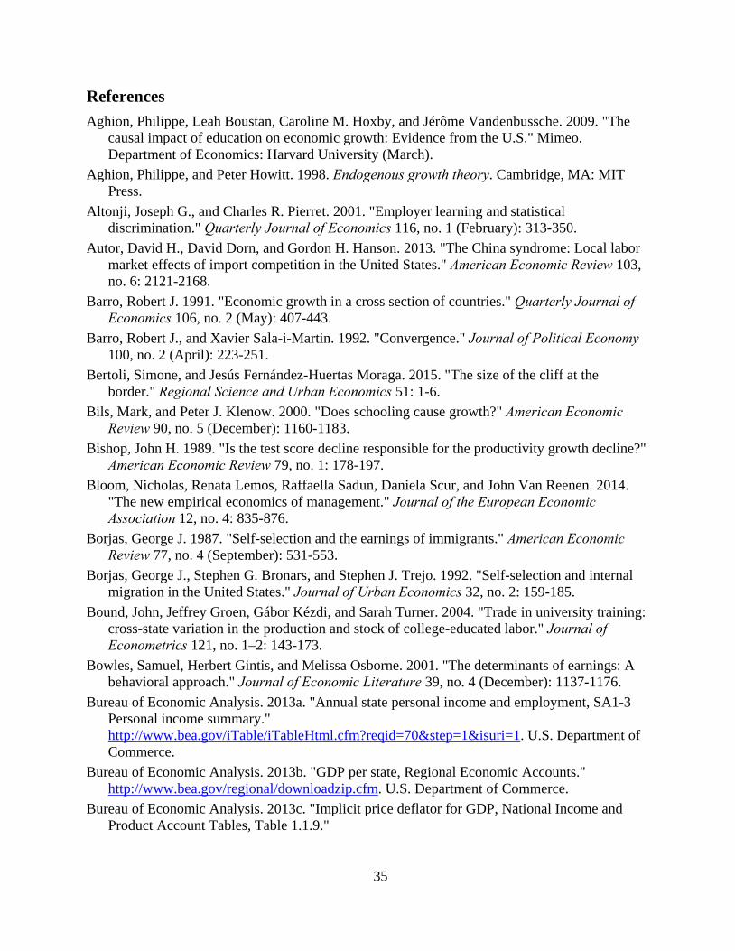
35

References Aghion, Philippe, Leah Boustan, Caroline M. Hoxby, and Jérôme Vandenbussche. 2009. "The

causal impact of education on economic growth: Evidence from the U.S." Mimeo. Department of Economics: Harvard University (March).

Aghion, Philippe, and Peter Howitt. 1998. Endogenous growth theory. Cambridge, MA: MIT Press.

Altonji, Joseph G., and Charles R. Pierret. 2001. "Employer learning and statistical discrimination." Quarterly Journal of Economics 116, no. 1 (February): 313-350.

Autor, David H., David Dorn, and Gordon H. Hanson. 2013. "The China syndrome: Local labor market effects of import competition in the United States." American Economic Review 103, no. 6: 2121-2168.

Barro, Robert J. 1991. "Economic growth in a cross section of countries." Quarterly Journal of Economics 106, no. 2 (May): 407-443.

Barro, Robert J., and Xavier Sala-i-Martin. 1992. "Convergence." Journal of Political Economy 100, no. 2 (April): 223-251.

Bertoli, Simone, and Jesús Fernández-Huertas Moraga. 2015. "The size of the cliff at the border." Regional Science and Urban Economics 51: 1-6.

Bils, Mark, and Peter J. Klenow. 2000. "Does schooling cause growth?" American Economic Review 90, no. 5 (December): 1160-1183.

Bishop, John H. 1989. "Is the test score decline responsible for the productivity growth decline?" American Economic Review 79, no. 1: 178-197.

Bloom, Nicholas, Renata Lemos, Raffaella Sadun, Daniela Scur, and John Van Reenen. 2014. "The new empirical economics of management." Journal of the European Economic Association 12, no. 4: 835-876.

Borjas, George J. 1987. "Self-selection and the earnings of immigrants." American Economic Review 77, no. 4 (September): 531-553.

Borjas, George J., Stephen G. Bronars, and Stephen J. Trejo. 1992. "Self-selection and internal migration in the United States." Journal of Urban Economics 32, no. 2: 159-185.

Bound, John, Jeffrey Groen, Gábor Kézdi, and Sarah Turner. 2004. "Trade in university training: cross-state variation in the production and stock of college-educated labor." Journal of Econometrics 121, no. 1–2: 143-173.

Bowles, Samuel, Herbert Gintis, and Melissa Osborne. 2001. "The determinants of earnings: A behavioral approach." Journal of Economic Literature 39, no. 4 (December): 1137-1176.

Bureau of Economic Analysis. 2013a. "Annual state personal income and employment, SA1-3 Personal income summary." http://www.bea.gov/iTable/iTableHtml.cfm?reqid=70&step=1&isuri=1. U.S. Department of Commerce.

Bureau of Economic Analysis. 2013b. "GDP per state, Regional Economic Accounts." http://www.bea.gov/regional/downloadzip.cfm. U.S. Department of Commerce.

Bureau of Economic Analysis. 2013c. "Implicit price deflator for GDP, National Income and Product Account Tables, Table 1.1.9."

36

http://www.bea.gov/iTable/iTable.cfm?reqid=9&step=3&isuri=1&903=13#reqid=9&step=3&isuri=1&903=13. U.S. Department of Commerce.

Card, David. 1999. "The causal effect of education on earnings." In Handbook of Labor Economics, edited by Orley Ashenfelter and David Card. Amsterdam: North-Holland: 1801-1863.

Card, David. 2001. "Estimating the return to schooling: Progress on some persistent econometric problems." Econometrica 69, no. 5 (September): 1127-1160.

Card, David, and Alan B. Krueger. 1992. "Does school quality matter? Returns to education and the characteristics of public schools in the United States." Journal of Political Economy 100, no. 1 (February): 1-40.

Caselli, Francesco. 2005. "Accounting for cross-country income differences." In Handbook of Economic Growth, edited by Philippe Aghion and Steven N. Durlauf. Amsterdam: North Holland: 679-741.

Caselli, Francesco. 2014. "The Latin American efficiency gap." CFM Discussion Paper 2014-21. London: Centre for Macroeconomics.

Caselli, Francesco. 2016. "The Latin American efficiency gap." In Understanding the Income and Efficiency Gap in Latin America and the Caribbean, edited by Jorge Thompson Araujo, Ekaterina Vostroknutova, Konstantin M. Wacker, and Mateo Clavijo. Washington, DC: World Bank: 33-56.

Chetty, Raj, John N. Friedman, Nathaniel Hilger, Emmanuel Saez, Diane Whitmore Schanzenbach, and Danny Yagan. 2011. "How does your kindergarten classroom affect your earnings? Evidence from Project STAR." Quarterly Journal of Economics 126, no. 4 (November): 1593-1660.

Chiswick, Barry R. 1999. "Are immigrants favorably self-selected?" American Economic Review 89, no. 2 (May): 181-185.

Ciccone, Antonio, and Elias Papaioannou. 2009. "Human capital, the structure of production, and growth." Review of Economics and Statistics 91, no. 1 (February): 66-82.

Coulson, Andrew J. 2014. "Drawing meaningful trends from the SAT." Cato Working Papers Washington, DC: Cato Institute (March).

Dahl, Gordon B. 2002. "Mobility and the return to education: Testing a Roy model with multiple markets." Econometrica 70, no. 6: 2367-2420.

Docquier, Frédéric, B. Lindsay Lowell, and Abdeslam Marfouk. 2009. "A gendered assessment of highly skilled emigration." Population and Development Review 35, no. 2: 297-321.

Economist. 2013. How to stop companies and people dodging tax, in Delaware as well as Grand Cayman. The Economist, February 16.

Erosa, Andrés, Tatyana Koreshkova, and Diego Restuccia. 2010. "How important is human capital? A quantitative theory assessment of world income inequality." Review of Economic Studies 77, no. 4 (October): 1421-1449.

Evans, Paul, and Georgios Karras. 2006. "Do economies converge? Evidence from a panel of U.S. states." Review of Economics and Statistics 78, no. 3: 384-388.

Gennaioli, Nicola, Rafael La Porta, Florencio Lopez-de-Silanes, and Andrei Shleifer. 2013. "Human capital and regional development." Quarterly Journal of Economics 128, no. 1 (February): 105-164.

37

Glaeser, Edward L., Giacomo A. M. Ponzetto, and Kristina Tobio. 2014. "Cities, skills and regional change." Regional Studies 48, no. 1: 7-43.

Glaeser, Edward L., and Albert Saiz. 2004. "The rise of the skilled city." Brookings-Wharton Papers on Urban Affairs 5: 47-105.

Goldin, Claudia, and Lawrence F. Katz. 2008. The race between education and technology. Cambridge, MA: Harvard University Press.

Graham, Amy E., and Thomas A. Husted. 1993. "Understanding state variations in SAT scores." Economics of Education Review 12, no. 3 (September): 197-202.

Grogger, Jeffrey, and Gordon H. Hanson. 2011. "Income maximization and the selection and sorting of international migrants." Journal of Development Economics 95, no. 1: 42-57.

Gundlach, Erich, Desmond Rudman, and Ludger Woessmann. 2002. "Second thoughts on development accounting." Applied Economics 34, no. 11: 1359-1369.

Haider, Steven, and Gary Solon. 2006. "Life-cycle variation in the association between current and lifetime earnings." American Economic Review 96, no. 4: 1308-1320.

Hall, Robert E., and Charles I. Jones. 1999. "Why do some countries produce so much more output per worker than others?" Quarterly Journal of Economics 114, no. 1: 83-116.

Hanushek, Eric A. 2003. "The failure of input-based schooling policies." Economic Journal 113, no. 485 (February): F64-F98.

Hanushek, Eric A. 2011. "The economic value of higher teacher quality." Economics of Education Review 30, no. 3 (June): 466-479.

Hanushek, Eric A., and Dennis D. Kimko. 2000. "Schooling, labor force quality, and the growth of nations." American Economic Review 90, no. 5 (December): 1184-1208.

Hanushek, Eric A., Paul E. Peterson, and Ludger Woessmann. 2013. Endangering prosperity: A global view of the American school. Washington, DC: Brookings Institution Press.

Hanushek, Eric A., Jens Ruhose, and Ludger Woessmann. 2015. "Economic gains for U.S. states from educational reform." NBER Working Paper 21770. Cambridge, MA: National Bureau of Economic Research (December).

Hanushek, Eric A., Guido Schwerdt, Simon Wiederhold, and Ludger Woessmann. 2015. "Returns to skills around the world: Evidence from PIAAC." European Economic Review 73: 103-130.

Hanushek, Eric A., and Ludger Woessmann. 2008. "The role of cognitive skills in economic development." Journal of Economic Literature 46, no. 3 (September): 607-668.

Hanushek, Eric A., and Ludger Woessmann. 2012a. "Do better schools lead to more growth? Cognitive skills, economic outcomes, and causation." Journal of Economic Growth 17, no. 4 (December): 267-321.

Hanushek, Eric A., and Ludger Woessmann. 2012b. "Schooling, educational achievement, and the Latin American growth puzzle." Journal of Development Economics 99, no. 2 (November): 497-512.

Hanushek, Eric A., and Lei Zhang. 2009. "Quality-consistent estimates of international schooling and skill gradients." Journal of Human Capital 3, no. 2 (Summer): 107-143.

Heckman, James J., John Eric Humphries, and Nicholas S. Mader. 2011. "The GED." In Handbook of the Economics of Education, edited by Eric A. Hanushek, Stephen Machin, and Ludger Woessmann. Amsterdam: North Holland: 423-483.

38

Heckman, James J., Anne Layne-Farrar, and Petra Todd. 1996. "Human capital pricing equations with an application to estimating the effect of schooling quality on earnings." Review of Economics and Statistics 78, no. 4 (November): 562-610.

Hendricks, Lutz. 2002. "How important is human capital for development? Evidence from immigrant earnings." American Economic Review 92, no. 1 (March): 198-219.

Higgins, Matthew J., Daniel Levy, and Andrew T. Young. 2006. "Growth and convergence across the United States: Evidence from county-level data." Review of Economics and Statistics 88, no. 4: 671-681.

Hsieh, Chang-Tai, and Peter J. Klenow. 2010. "Development accounting." American Economic Journal: Macroeconomics 2, no. 1: 207-223.

Jaeger, David A. 1997. "Reconciling the old and new Census Bureau education questions: Recommendations for researchers." Journal of Business and Economic Statistics 15, no. 3 (July): 300-309.

Jones, Benjamin F. 2014. "The human capital stock: A generalized approach." American Economic Review 104, no. 11: 3752-77.

Jovanovic, Boyan. 1979. "Job matching and the theory of turnover." Journal of Political Economy 87, no. 5 (October): 972-990.

Kaarsen, Nicolai. 2014. "Cross-country differences in the quality of schooling." Journal of Development Economics 107: 215-224.

Kennan, John. 2015. "Spatial variation in higher education financing and the supply of college graduates." NBER Working Paper 21065. Cambridge, MA: National Bureau of Economic Research (November).

Klenow, Peter J., and Andres Rodriquez-Clare. 1997. "The neoclassical revival in growth economics: Has it gone too far?" In NBER Macroeconomics Annual 1997, edited by Ben S. Bernancke and Julio J. Rotemberg. Cambridge, MA: MIT Press: 83-103.

Lazear, Edward P. 2003. "Teacher incentives." Swedish Economic Policy Review 10, no. 3: 179-214.

Lucas, Robert E., Jr. 1988. "On the mechanics of economic development." Journal of Monetary Economics 22, no. 1 (July): 3-42.

Mankiw, N. Gregory, David Romer, and David Weil. 1992. "A contribution to the empirics of economic growth." Quarterly Journal of Economics 107, no. 2 (May): 407-437.

Manuelli, Rodolfo E., and Ananth Seshadri. 2014. "Human capital and the wealth of nations." American Economic Review 104, no. 9: 2736-62.

Mincer, Jacob. 1974. Schooling, experience, and earnings. New York: NBER. Mulligan, Casey B. 1999. "Galton versus the human capital approach to inheritance." Journal of

Political Economy 107, no. 6, pt. 2 (December): S184-S224. Murnane, Richard J., John B. Willett, Yves Duhaldeborde, and John H. Tyler. 2000. "How

important are the cognitive skills of teenagers in predicting subsequent earnings?" Journal of Policy Analysis and Management 19, no. 4 (Fall): 547-568.

Murnane, Richard J., John B. Willett, and Frank Levy. 1995. "The growing importance of cognitive skills in wage determination." Review of Economics and Statistics 77, no. 2 (May): 251-266.

39

National Center for Education Statistics. 2014. National Assessment of Educational Progress (NAEP). http://nces.ed.gov/nationsreportcard/naepdata/.

Neal, Derek, and William R. Johnson. 1996. "The role of pre-market factors in black-white differences." Journal of Political Economy 104, no. 5 (October): 869-895.

Nelson, Richard R., and Edmund Phelps. 1966. "Investment in humans, technology diffusion and economic growth." American Economic Review 56, no. 2 (May): 69-75.

Ortega, Francesc, and Giovanni Peri. 2013. "The effect of income and immigration policies on international migration." Migration Studies 1, no. 1 (March): 47-74.

Parey, Matthias, Jens Ruhose, Fabian Waldinger, and Nicolai Netz. 2016. "The selection of high-skilled emigrants." Review of Economics and Statistics: forthcoming.

Peri, Giovanni. 2012. "The effect of immigration on productivity: Evidence from U.S. states." Review of Economics and Statistics 94, no. 1 (February): 348-358.

Rappaport, Jordan, and Jeffrey D. Sachs. 2003. "The United States as a coastal nation." Journal of Economic Growth 8, no. 1: 5-46.

Romer, Paul. 1990. "Endogenous technological change." Journal of Political Economy 99, no. 5, pt. II: S71-S102.

Ruggles, Steven, J. Trent Alexander, Katie Genadek, Ronald Goeken, Matthew B. Schroeder, and Matthew Sobek. 2010. "Integrated Public Use Microdata Series: Version 5.0 [Machine-readable database]. University of Minnesota.

Schoellman, Todd. 2012. "Education quality and development accounting." Review of Economic Studies 79, no. 1 (January): 388-417.

Tamura, Robert. 2001. "Teachers, growth, and convergence." Journal of Political Economy 109, no. 5: 1021-1059.

Tamura, Robert, Curtis Simon, and Kevin M. Murphy. 2016. "Black and white fertility, differential baby booms: The value of equal education opportunity." Journal of Demographic Economics 82, no. 1: 27-109.

Turner, Chad, Robert Tamura, and Sean E. Mulholland. 2013. "How important are human capital, physical capital and total factor productivity for determining state economic growth in the United States, 1840–2000?" Journal of Economic Growth 18, no. 4 (December): 319-371.

Turner, Chad, Robert Tamura, Sean E. Mulholland, and Scott Baier. 2007. "Education and income of the states of the United States: 1840–2000." Journal of Economic Growth 12, no. 2 (June): 101-158.

Vogl, Tom S. 2014. "Height, skills, and labor market outcomes in Mexico." Journal of Development Economics 107(March): 84-96.

You, Hye Mi. 2014. "The contribution of rising school quality to U.S. economic growth." Journal of Monetary Economics 63(April): 95-106.

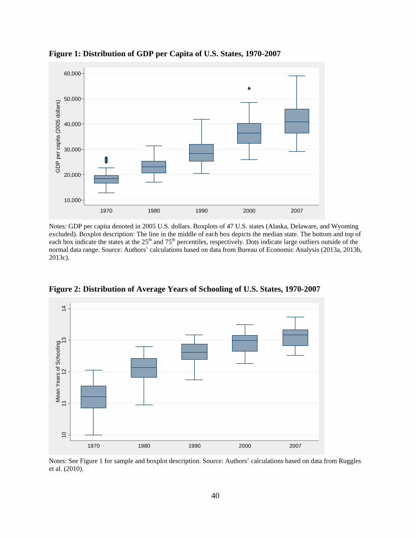
40

Figure 1: Distribution of GDP per Capita of U.S. States, 1970-2007

Notes: GDP per capita denoted in 2005 U.S. dollars. Boxplots of 47 U.S. states (Alaska, Delaware, and Wyoming excluded). Boxplot description: The line in the middle of each box depicts the median state. The bottom and top of each box indicate the states at the 25th and 75th percentiles, respectively. Dots indicate large outliers outside of the normal data range. Source: Authors’ calculations based on data from Bureau of Economic Analysis (2013a, 2013b, 2013c). Figure 2: Distribution of Average Years of Schooling of U.S. States, 1970-2007

Notes: See Figure 1 for sample and boxplot description. Source: Authors’ calculations based on data from Ruggles et al. (2010).

10,000

20,000

30,000

40,000

50,000

60,000

GD

P pe

r cap

ita (2

005

dolla

rs)

1970 1980 1990 2000 2007

1011

1213

14M

ean

Year

s of

Sch

oolin

g

1970 1980 1990 2000 2007

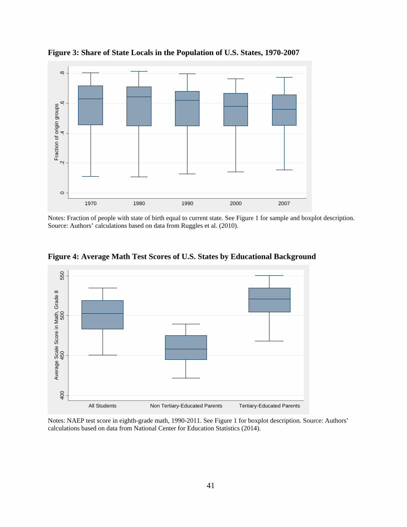
41

Figure 3: Share of State Locals in the Population of U.S. States, 1970-2007

Notes: Fraction of people with state of birth equal to current state. See Figure 1 for sample and boxplot description. Source: Authors’ calculations based on data from Ruggles et al. (2010). Figure 4: Average Math Test Scores of U.S. States by Educational Background

Notes: NAEP test score in eighth-grade math, 1990-2011. See Figure 1 for boxplot description. Source: Authors’ calculations based on data from National Center for Education Statistics (2014).

0.2

.4.6

.8Fr

actio

n of

orig

in g

roup

s

1970 1980 1990 2000 2007

400

450

500

550

Aver

age

Scal

e Sc

ore

in M

ath,

Gra

de 8

All Students Non Tertiary-Educated Parents Tertiary-Educated Parents

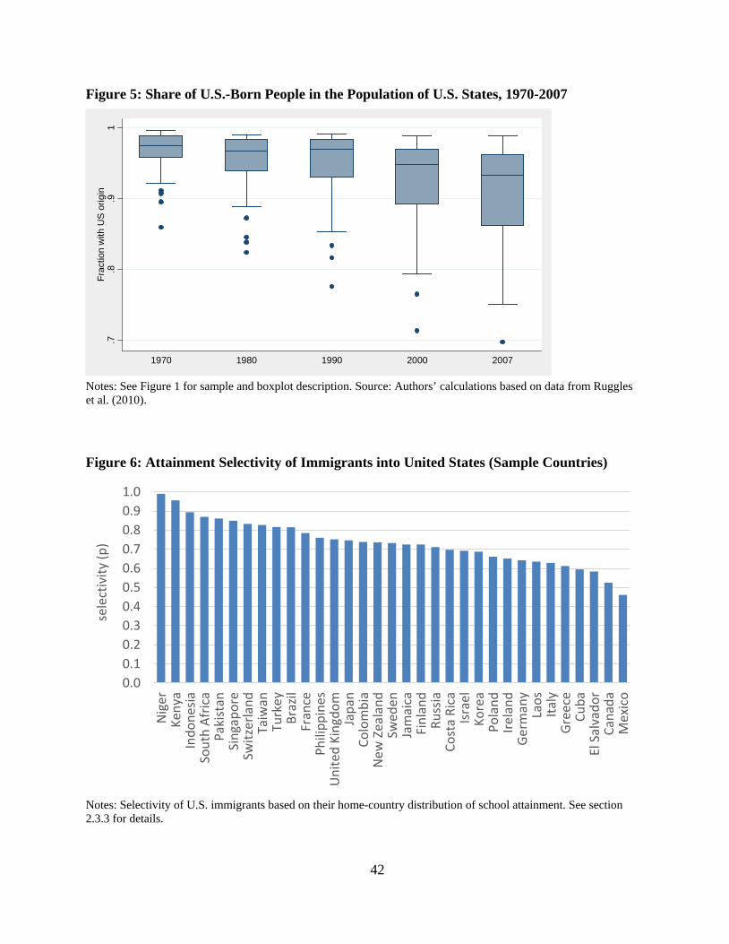
42

Figure 5: Share of U.S.-Born People in the Population of U.S. States, 1970-2007

Notes: See Figure 1 for sample and boxplot description. Source: Authors’ calculations based on data from Ruggles et al. (2010). Figure 6: Attainment Selectivity of Immigrants into United States (Sample Countries)

Notes: Selectivity of U.S. immigrants based on their home-country distribution of school attainment. See section 2.3.3 for details.

.7.8

.91

Frac

tion

with

US

orig

in

1970 1980 1990 2000 2007

0.00.10.20.30.40.50.60.70.80.91.0

Nig

erKe

nya

Indo

nesia

Sout

h Af

rica

Paki

stan

Sing

apor

eSw

itzer

land

Taiw

anTu

rkey

Braz

ilFr

ance

Phili

ppin

esU

nite

d Ki

ngdo

mJa

pan

Colo

mbi

aN

ew Z

eala

ndSw

eden

Jam

aica

Finl

and

Russ

iaCo

sta

Rica

Isra

elKo

rea

Pola

ndIre

land

Germ

any

Laos

Italy

Gree

ceCu

baEl

Sal

vado

rCa

nada

Mex

ico

sele

ctiv

ity (p

)

43

Figure 7: Net Gain in Knowledge Capital from Migration

Notes: Net gain in knowledge capital from migration: ratio of the actual returns-weighted knowledge capital measure (calculated from equation (1)) over a knowledge capital without any migration. See Appendix Table A1 for details.

44

Figure 8: Years of Schooling and GDP per Capita across U.S. States, 2007

Source: Authors’ calculations based on data from Bureau of Economic Analysis (2013a, 2013b, 2013c) and Ruggles et al. (2010). Figure 9: Cognitive Skills and GDP per Capita across U.S. States, 2007

Source: Authors’ calculations based on data from Bureau of Economic Analysis (2013a, 2013b, 2013c), Ruggles et al. (2010), and National Center for Education Statistics (2014).

AL

AZ

AR

CACO

CT

FLGA

HI

ID

IL

IN

IAKS

KY

LA

ME

MD

MA

MI

MN

MS

MO

MT

NE

NV

NH

NJ

NM

NY

NC ND

OH

OK

OR

PA

RI

SC

SD

TN

TX

UT

VT

VAWA

WV

WI

10.2

10.4

10.6

10.8

11.0

Log

GD

P pe

r cap

ita ($

2005

), 20

07

12.5 13 13.5 14

Mean years of schooling, 2007

AL

AZ

AR

CACO

CT

FLGA

HI

ID

IL

IN

IAKS

KY

LA

ME

MD

MA

MI

MN

MS

MO

MT

NE

NV

NH

NJ

NM

NY

NC ND

OH

OK

OR

PA

RI

SC

SD

TN

TX

UT

VT

VA WA

WV

WI

10.2

10.4

10.6

10.8

11.0

Log

GD

P pe

r cap

ita ($

2005

), 20

07

380 400 420 440 460 480

Test score

45

Figure 10: Growth Accounting by State, 1970-2007

Notes: Growth accounting results by U.S. states. Contribution of changes in years of schooling and in estimated test scores to the average annual rate of growth in GDP per capita in 1970-2007. See Table A8 in the Online Appendix for details. Source: Authors’ calculations based on data from Bureau of Economic Analysis (2013a, 2013b, 2013c), Ruggles et al. (2010), and National Center for Education Statistics (2014).

0.0

0.5

1.0

1.5

2.0

2.5

3.0

Sout

h D

akot

aN

orth

Dak

ota

Con

nect

icut

Virg

inia

Col

orad

oM

assa

chus

etts

New

Ham

pshi

reTe

xas

Geo

rgia

Kan

sas

Neb

rask

aLo

uisi

ana

Mar

ylan

dN

ew Je

rsey

Uta

hA

rkan

sas

Min

neso

taM

issi

ssip

piA

laba

ma

Iow

aR

hode

Isla

ndO

rego

nN

orth

Car

olin

aSo

uth

Car

olin

aTe

nnes

see

Okl

ahom

aW

ashi

ngto

nM

aine

Wis

cons

inFl

orid

aC

alifo

rnia

New

Yor

kM

onta

naPe

nnsy

lvan

iaA

rizon

aIll

inoi

sId

aho

Indi

ana

New

Mex

ico

Ver

mon

tM

isso

uri

Ken

tuck

yO

hio

Nev

ada

Wes

t Virg

inia

Haw

aii

Mic

higa

n

Ann

ual a

vera

ge G

DP

per c

apita

gro

wth

, 197

0-20

07

Years of schooling Test scores Total annual average GDP per capita growth

46

Table 1: Correlations among Test Score Measures, 2007

Test score specification 1 2 3 4 5 6

1 Baseline: local average adjusted for interstate migrants 1

2 + Adjustment of locals by education category 0.990 1

3 + Adjustment of interstate migrants by education category 0.984 0.996 1

4 + Adjustment of international migrants scores by selectivity 0.914 0.945 0.959 1

5 Age adjustment with extrapolation of NAEP trends by education category 0.803 0.848 0.862 0.922 1

6 Age adjustment with projection from SAT scores 0.668 0.704 0.707 0.746 0.911 1

Notes: Test scores refer to eighth-grade math. Locals are all persons who report a state of birth equal to the current state of residence. Interstate migrants report another state of birth than state of residence. International migrants report another country of birth than the United States. “By education category” indicates that individuals with/without university education are assigned the test scores of children of parents with/without university education.

47

Table 2: Development Accounting Results with Different Test Score Specifications, 2007

Notes: Development accounting results for 47 U.S. states with different test score specifications. Test scores refer to eighth-grade math. Locals are all persons who report a state of birth equal to the current state of residence. Interstate migrants report another state of birth than state of residence. International migrants report another country of birth than the United States. “By education category” indicates that individuals with/without university education are assigned the test scores of children of parents with/without university education. Calculations assume a return of w=0.17 per standard deviation in test scores and a return of r=0.08 per year of schooling. Bootstrapped standard errors in parentheses with 1,000 replications. Significance levels: * p < 0.10, ** p < 0.05, *** p < 0.01.

Covariance Measure Five-State Measure

Test score specification Total know-ledge capital

Test scores

Years of schooling

Total know-ledge capital

Test scores

Years of schooling

Baseline: local average adjusted for interstate migrants 0.150*** (0.045)

0.057** (0.025)

0.093*** (0.023)

0.213 0.093 0.120

+ Adjustment of locals by education category 0.159*** (0.043)

0.066*** (0.024)

0.093*** (0.023)

0.221 0.101 0.120

+ Adjustment of interstate migrants by education category 0.169*** (0.043)

0.076*** (0.024)

0.093*** (0.023)

0.231 0.111 0.120

+ Adjustment of international migrants by selectivity-adjusted home country scores

0.190*** (0.041)

0.097*** (0.022)

0.093*** (0.023)

0.255 0.135 0.120

+ Backward projection of NAEP scores by age 0.215*** (0.045)

0.122*** (0.029)

0.093*** (0.023)

0.295 0.175 0.120

+ Backward projection of NAEP scores by age and parental education

0.228*** (0.044)

0.135*** (0.028)

0.093*** (0.023)

0.306 0.186 0.120

48

Table 3: Development Accounting Results with Alternative Projections of Cognitive Skills from SAT Scores by Age, 2007

Extrapolation of NAEP trends Projection from state SAT scores

Linear state trend before first observed score 0.122*** (0.029)

0.124*** (0.042)

Constant before first observed score 0.114*** (0.026)

0.115*** (0.038)

Notes: Development accounting results for 47 U.S. states with different test score specifications based on projections by age. First scores are observed in 1978 in the case of national NAEP and in 1968 in the case of SAT. Test scores refer to eighth-grade math. Calculations assume a return of w=0.17 per standard deviation in test scores and a return of r=0.08 per year of schooling. Bootstrapped standard errors in parentheses with 1,000 replications. Significance levels: * p < 0.10, ** p < 0.05, *** p < 0.01.

49

Table 4: Sensitivity to Alternative Return Parameters

Notes: Development accounting results (covariance measure) for 47 U.S. states with different assumptions on the return w per standard deviation in test scores and the return r per year of schooling. Test score specification adjusts locals and interstate migrants by age-education category based on extrapolation of NAEP trends by education category and international migrants with selectivity-adjusted home country scores of birth. Test scores refer to eighth-grade math. Bootstrapped standard errors in parentheses with 1,000 replications. Significance levels: * p < 0.10, ** p < 0.05, *** p < 0.01.

r w Total knowledge

capital Test

scores Years of schooling

Baseline 0.08 0.17 0.228*** (0.044)

0.135*** (0.028)

0.093*** (0.023)

Alternative returns to test scores 0.08 0.14 0.204*** (0.040)

0.111*** (0.023)

0.093*** (0.023)

0.08 0.20 0.252*** (0.049)

0.159*** (0.033)

0.093*** (0.023)

Alternative returns to years of schooling 0.06 0.17 0.205*** (0.040)

0.135*** (0.028)

0.070*** (0.017)

0.10 0.17 0.252*** (0.049)

0.135*** (0.028)

0.117*** (0.028)

Pure skills 0.0 0.28 0.222*** (0.046)

0.222*** (0.046)

0.000

Returns to years of schooling estimated from IPUMS 2007:

Uniform returns estimate 0.124 0.17 0.280*** (0.055)

0.135*** (0.028)

0.145*** (0.035)

Schooling level-specific returns estimates rnon-tertiary = 0.057 rtertiary = 0.157

0.17 0.315*** (0.052)

0.135*** (0.028)

0.180*** (0.032)

Price-adjusted GDP per capita 0.08 0.17 0.229*** (0.088)

0.147*** (0.054)

0.082*** (0.040)

Unadjusted school-attainment selectivity 0.08 0.17 0.181*** (0.047)

0.088*** (0.029)

0.093*** (0.023)

International migrants at 90th percentile 0.08 0.17 0.226*** (0.044)

0.133*** (0.029)

0.093*** (0.023)

50

Table 5: Growth Accounting Results

Average annual growth rate of

Absolute change in Estimated

Average annual growth rate accounted for by Percent of total growth

real GDP per

capita (percent) years of

schooling annual change in test scores

Total know-ledge capital

Test scores

Years of schooling Total know-

ledge capital Test

scores Years of schooling

1970-1980 2.17 0.89 3.16 0.83 0.36 0.47 38.2 16.5 21.7

1980-1990 2.39 0.56 3.16 0.66 0.36 0.30 27.5 15.0 12.5

1990-2000 2.47 0.29 3.16 0.51 0.36 0.15 20.7 14.5 6.3

2000-2007 1.52 0.22 3.16 0.52 0.36 0.16 34.4 23.6 10.8

1970-2007 2.19 1.95 3.16 0.64 0.36 0.28 29.2 16.4 12.9

1970-2000 2.35 1.74 3.16 0.67 0.36 0.31 28.4 15.3 13.2

1970-1990 2.28 1.45 3.16 0.74 0.36 0.39 32.6 15.7 16.9

1990-2007 2.08 0.50 3.16 0.52 0.36 0.16 24.9 17.2 7.6

Notes: Estimated annual change in test scores: in percent of a standard deviation, obtained from a regression of test scores (NAEP scores projected based on participation-corrected SAT scores as derived in section 2.3.4) on years for each state, 1968-2011.

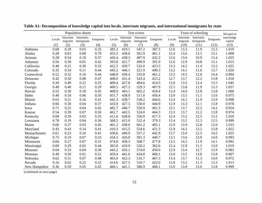
51

Table A1: Decomposition of knowledge capital into locals, interstate migrants, and international immigrants by state

Population shares Test scores Years of schooling Net gain in

Locals Interstate migrants

Internatio. Immigrants Emigrants Locals Interstate

migrants Internatio. immigrants Emigrants Locals Interstate

migrants Internatio. immigrants Emigrants knowledge

capital (1) (2) (3) (4) (5) (6) (7) (8) (9) (10) (11) (12) (13) Alabama 0.68 0.29 0.03 0.35 385.3 419.1 547.2 387.5 12.6 13.3 11.9 13.3 1.019 Alaska 0.28 0.63 0.08 0.70 455.5 438.6 561.9 461.1 12.4 13.6 12.5 13.1 1.008 Arizona 0.28 0.54 0.18 0.37 426.4 438.3 497.9 432.2 12.6 13.6 10.9 13.4 1.025 Arkansas 0.56 0.39 0.05 0.42 393.8 421.7 499.9 391.9 12.6 12.9 10.8 13.1 1.015 California 0.48 0.21 0.30 0.33 422.5 439.7 532.0 423.5 13.3 14.2 11.4 13.5 1.025 Colorado 0.35 0.54 0.11 0.44 445.2 446.1 521.9 449.3 13.2 14.1 11.6 13.7 1.020 Connecticut 0.52 0.32 0.16 0.44 448.8 439.4 535.8 461.2 13.5 14.5 12.6 14.4 0.994 Delaware 0.42 0.50 0.08 0.47 408.6 431.4 543.4 423.2 12.7 13.7 12.2 13.8 1.018 Florida 0.30 0.49 0.22 0.35 408.4 427.8 494.6 414.5 12.8 13.5 12.4 13.5 1.045 Georgia 0.49 0.40 0.11 0.29 400.5 427.3 529.3 407.9 12.5 13.8 11.9 13.3 1.057 Hawaii 0.52 0.30 0.18 0.45 408.9 443.1 602.2 418.4 13.4 14.0 12.8 13.8 1.060 Idaho 0.40 0.54 0.06 0.50 451.7 438.9 511.8 456.4 13.0 13.5 11.1 13.6 0.975 Illinois 0.63 0.21 0.16 0.41 441.3 438.7 538.2 444.6 13.4 14.1 11.9 13.9 0.998 Indiana 0.66 0.30 0.04 0.37 433.9 427.5 530.0 444.9 12.9 13.3 12.1 13.8 0.978 Iowa 0.71 0.25 0.04 0.45 482.7 446.7 550.9 491.5 13.1 13.7 12.2 14.2 0.954 Kansas 0.54 0.39 0.07 0.50 461.7 442.5 524.0 464.3 13.3 13.7 11.2 13.8 0.974 Kentucky 0.68 0.29 0.03 0.35 411.6 428.8 556.9 417.3 12.4 13.2 12.5 13.2 1.010 Louisiana 0.78 0.19 0.04 0.36 368.5 415.0 532.4 379.3 12.4 13.2 12.3 13.5 0.999 Maine 0.60 0.37 0.03 0.45 461.2 438.6 601.2 465.1 12.9 13.9 12.8 12.6 1.033 Maryland 0.43 0.43 0.14 0.41 410.3 415.5 554.6 421.3 12.9 14.3 13.2 13.8 1.052 Massachusetts 0.61 0.23 0.16 0.41 438.6 449.9 557.2 442.9 13.7 15.0 12.5 14.2 1.025 Michigan 0.75 0.19 0.07 0.33 434.3 426.0 581.3 440.7 13.1 13.6 12.9 14.0 0.993 Minnesota 0.66 0.27 0.07 0.31 474.0 458.3 568.7 477.8 13.5 14.2 11.9 14.1 0.992 Mississippi 0.69 0.29 0.02 0.44 365.0 410.9 526.2 362.6 12.4 12.9 11.5 13.0 1.019 Missouri 0.64 0.33 0.04 0.36 443.2 435.1 574.0 450.0 12.9 13.4 12.7 13.9 0.983 Montana 0.49 0.50 0.01 0.52 459.4 441.0 634.8 469.1 13.0 13.5 13.0 13.8 0.967 Nebraska 0.62 0.31 0.07 0.48 463.0 452.3 516.7 467.5 13.4 13.7 11.3 14.0 0.972 Nevada 0.16 0.62 0.22 0.52 414.6 427.5 510.7 422.0 12.8 13.2 11.3 13.3 1.013 New Hampshire 0.36 0.59 0.05 0.45 460.1 441.1 586.9 468.1 13.0 13.9 13.6 13.8 0.999

(continued on next page)

52

Table A1 (continued)

Population shares Test scores Years of schooling Net gain in

Locals Interstate migrants

Internatio. Immigrants Emigrants Locals Interstate

migrants Internatio. immigrants Emigrants Locals Interstate

migrants Internatio. immigrants Emigrants knowledge

capital (1) (2) (3) (4) (5) (6) (7) (8) (9) (10) (11) (12) (13) New Jersey 0.49 0.27 0.24 0.45 442.0 434.8 548.7 449.5 13.4 14.2 12.9 14.2 1.013 New Mexico 0.47 0.43 0.10 0.48 408.8 433.6 496.7 416.4 12.6 13.6 10.3 13.3 1.018 New York 0.62 0.13 0.25 0.45 428.3 439.7 549.9 435.5 13.5 14.4 12.3 14.3 1.008 North Carolina 0.54 0.38 0.08 0.28 389.1 432.4 517.6 394.1 12.7 13.7 11.5 13.5 1.052 North Dakota 0.68 0.30 0.02 0.58 475.5 459.6 592.8 479.7 13.4 13.7 13.1 14.1 0.968 Ohio 0.74 0.22 0.04 0.35 426.7 426.0 582.9 435.1 13.0 13.5 13.4 13.9 0.989 Oklahoma 0.56 0.38 0.06 0.41 435.7 426.3 526.5 441.9 12.9 13.1 11.2 13.7 0.973 Oregon 0.41 0.49 0.10 0.41 446.4 435.3 541.6 452.0 13.1 13.8 11.2 13.6 0.997 Pennsylvania 0.74 0.19 0.06 0.35 438.4 430.1 558.1 448.5 13.1 13.8 12.9 14.2 0.984 Rhode Island 0.58 0.27 0.15 0.48 425.5 445.1 522.6 436.3 13.1 14.1 11.2 14.1 0.987 South Carolina 0.56 0.39 0.05 0.33 397.3 423.8 537.4 406.2 12.5 13.5 12.0 13.4 1.032 South Dakota 0.63 0.35 0.02 0.53 461.5 454.6 535.4 465.8 13.0 13.5 11.4 14.0 0.965 Tennessee 0.57 0.38 0.05 0.32 401.4 421.1 541.0 407.7 12.4 13.3 11.9 13.4 1.020 Texas 0.55 0.26 0.19 0.24 420.9 431.6 498.0 426.6 12.8 13.8 10.6 13.3 1.004 Utah 0.57 0.33 0.10 0.34 450.5 442.1 520.6 457.4 13.2 13.9 11.7 14.0 0.988 Vermont 0.48 0.49 0.03 0.46 438.2 445.5 619.1 449.1 12.8 14.4 13.5 13.7 1.041 Virginia 0.45 0.43 0.12 0.39 420.2 431.8 555.5 432.4 12.7 14.3 13.0 13.7 1.057 Washington 0.42 0.45 0.13 0.35 442.7 442.6 577.1 444.5 13.3 13.9 12.2 13.8 1.026 West Virginia 0.70 0.28 0.01 0.50 405.2 421.7 589.9 410.5 12.3 12.9 13.6 13.1 0.990 Wisconsin 0.70 0.26 0.05 0.31 466.1 441.8 537.9 476.4 13.2 13.7 12.1 14.4 0.968 Wyoming 0.38 0.58 0.03 0.62 456.0 445.0 532.9 458.0 13.0 13.4 12.0 13.7 0.974

Notes: Population shares in columns (1)-(3) add up to 1 for each state. Column (4): Share of the population born in this state that currently lives in another state. Column (13): Net gain in knowledge capital: ratio of the actual returns-weighted knowledge capital measure (calculated from equation (1)) over a knowledge capital without any migration.

Online Appendix 2

Appendix A: Construction of Years of Schooling Measures by State

We compile average years of educational attainment for each U.S. state from the Integrated

Public Use Microdata Series (IPUMS) data of the Minnesota Population Center (Ruggles et al.

(2010)). We concentrate on the working-age population between 20 and 65 years. We also drop

all respondents who are still in school at the time of the survey.

For the years 1970 to 2000, we use the 1 percent (1970) and 5 percent (1980, 1990, and

2000) random samples of the American population. The 1 percent sample has about 4 million

observations, the 5 percent samples have about 13 to 14 million observations. Beginning in the

year 2001, we use census data from the American Community Survey (ACS). The ACS provides

annual 1 percent random population samples (with smaller sample sizes between 2001 and

2004). The approximate sample size is 3 million observations each year. Survey weights in the

census and the ACS allow us to calculate measures that are representative for the U.S.

population.

Until 1980, the Census reported directly the years of schooling or highest grade level

completed of each individual. Beginning with the 1990 Census, the Census Bureau has changed

the coding of educational categories and reports degrees (Bachelor, Master, etc.) instead. To

translate the degree information into years of schooling, we use the estimates of average years of

schooling of each degree provided by Jaeger (1997).1

Substantial differences in the labor-market performance between GED holders and standard

high school graduates (Heckman, Humphries, and Mader (2011)) warrant a special treatment of

GED holders. Due to the weak labor-market position of GED holders, we assign them 10 rather

than 12 years of schooling.

Only the most recent survey waves identify GED holders in the Census data. We therefore

estimate a constant share of GED holders among all high-school graduates from the pooled ACS

2008-2010 samples. The pooled sample is restricted for each year to get approximately the same

age cohort of people aged 20-65. For example, for the year 2007, we use all people aged 21-66 in

ACS 2008, 22-67 in ACS 2009, and 23-68 in 2010; for the year 1990, we use all people aged 38-

83 in ACS 2008, 39-84 in ACS 2009, and 40-85 in ACS 2010. Note that 1940 is not adjusted

because the GED was introduced in 1942.

1 Some Census years only report educational categories that cover several years of schooling. For these years,

we assume the same fraction for this educational category as in the closest survey with full information.

Online Appendix 3

Overall, the GED adjustment affects the average years of schooling only very little, though.

In 2007, for example, 15 percent of those who would have received 12 years of schooling

otherwise are now assigned 10 years of schooling, reducing the mean of the average years of

schooling from 12.33 to 12.27 years. Put differently, accounting for GED holders raises the mean

share of those with less than 12 years of schooling from 22.6 percent to 26.7 percent.

Having computed the years of schooling of each individual i, the average years of schooling

S in state s at time t is then given by combining individual years of schooling by the weighted

share of individuals i with education level e in the state at the time:

𝑆𝑆𝑠𝑠𝑠𝑠 = ∑ ∑ 𝑝𝑝𝑝𝑝𝑝𝑝𝑠𝑠𝑝𝑝𝑝𝑝 w𝑝𝑝𝑒𝑒𝑒𝑒ℎ𝑠𝑠𝑠𝑠𝑖𝑖𝑖𝑖𝑖𝑖𝑖𝑖𝑖𝑖∑ 𝑝𝑝𝑝𝑝𝑝𝑝𝑠𝑠𝑝𝑝𝑝𝑝 𝑤𝑤𝑝𝑝𝑒𝑒𝑒𝑒ℎ𝑠𝑠𝑠𝑠𝑖𝑖𝑖𝑖𝑖𝑖𝑖𝑖

∗ 𝑦𝑦𝑦𝑦𝑦𝑦𝑦𝑦𝑦𝑦 𝑜𝑜𝑜𝑜 𝑦𝑦𝑠𝑠ℎ𝑜𝑜𝑜𝑜𝑜𝑜𝑜𝑜𝑜𝑜𝑜𝑜𝑝𝑝𝑝𝑝 (A1)

This yields the average years of schooling by state over time as shown in Figure 2.

Appendix B: Construction of Test Score Measures by State

As indicated in section 2.3 of the main text, our construction of cognitive skill measures for

each U.S. state proceeds in four steps. This appendix provides methodological details on each

step. First, we construct a constant measure of the mean test scores of students of each state

(Appendix B.1). Second, we adjust the test scores of the working-age population of each state for

interstate migration, thereby placing particular emphasis on the fact that interstate migration is

selective (Appendix B.2). Third, test scores are adjusted for immigration from other countries,

again with a special focus on selectivity (Appendix B.3). Fourth, we project test scores backward

in time to allow for age-varying test scores in each state (Appendix B.4).

B.1 Construction of Mean State Test Scores

The National Assessment of Educational Progress (NAEP) studies the educational

achievement of American students in grades four and eight in different subjects (National Center

for Education Statistics (2014)). In our main analysis, we focus on the mathematics score in

grade eight, on which we focus the following description. But as far as possible, we also

computed test scores based on reading and grade four, as well as on a combination of subjects

and grades.

Since 1990, NAEP math tests have been administered on a representative scale at the state

level every two to four years for most states. By 2003, test scores are available for all states.

Online Appendix 4

Adjustment of Pre-1996 Tests for Accommodation

Since 1996, NAEP allows students with disabilities and English language learners specific

accommodations to facilitate test participation. The NAEP test scores before 1996 (in 1990 and

1992) did not permit such accommodation, so that they have to be adjusted in order to be on a

common scale with the subsequent tests. Therefore, we rescale the pre-1996 tests as follows: For

1996, NAEP test scores and standard deviations are available for tests with and without

accommodation at the national level. By subtracting the 1996 U.S. mean without accommodation

from the state score and dividing by the 1996 U.S. standard deviation without accommodation,

we standardize test scores to mean 0 and standard deviation of 1. By multiplying the 1996 U.S.

standard deviation with accommodation and adding the 1996 U.S. mean with accommodation,

we bring each test score before 1996 to the same scale as the tests that permitted

accommodation.

That is, the pre-1996 waves are aligned to the post-1996 scale in the following way:

𝑦𝑦𝑠𝑠𝑜𝑜𝑦𝑦𝑦𝑦𝑠𝑠𝑠𝑠𝑎𝑎𝑎𝑎𝑎𝑎 = �

𝑠𝑠𝑠𝑠𝑝𝑝𝑝𝑝𝑝𝑝𝑖𝑖𝑖𝑖−𝑚𝑚𝑝𝑝𝑎𝑎𝑝𝑝𝑈𝑈𝑈𝑈,𝑖𝑖=1996𝑖𝑖𝑠𝑠𝑠𝑠𝑖𝑖 𝑖𝑖𝑠𝑠𝑠𝑠𝑠𝑠𝑖𝑖

𝑠𝑠𝑎𝑎𝑈𝑈𝑈𝑈,𝑖𝑖= 1996𝑖𝑖𝑠𝑠𝑠𝑠𝑖𝑖 𝑖𝑖𝑠𝑠𝑠𝑠𝑠𝑠𝑖𝑖 � ∗ 𝑦𝑦𝑠𝑠𝑈𝑈𝑈𝑈,𝑠𝑠= 1996

𝑝𝑝𝑝𝑝𝑤𝑤 𝑠𝑠𝑠𝑠𝑎𝑎𝑠𝑠𝑝𝑝 + 𝑚𝑚𝑦𝑦𝑦𝑦𝑜𝑜𝑈𝑈𝑈𝑈,𝑠𝑠=1996𝑝𝑝𝑝𝑝𝑤𝑤 𝑠𝑠𝑠𝑠𝑎𝑎𝑠𝑠𝑝𝑝 (B1)

where 𝑦𝑦𝑠𝑠𝑜𝑜𝑦𝑦𝑦𝑦𝑠𝑠𝑠𝑠 is the raw score (without accommodation) of state s at time t, mean refers to the

U.S. national mean, sd refers to the U.S. standard deviation, same scale refers to scores without

accommodation, and new scale refers to scores with accommodation.

Normalization of Scales to Base Year 2011

Next, we normalize each scale – eight-grade math, etc. – to have a mean of 500 and a

standard deviation of 100 in the common base year 2011. This is done by subtracting from each

test score the 2011 U.S. mean and dividing by the 2011 U.S. standard deviation and then

multiplying by 100 and adding 500:

𝑦𝑦𝑠𝑠𝑜𝑜𝑦𝑦𝑦𝑦𝑠𝑠𝑠𝑠𝑠𝑠𝑠𝑠𝑎𝑎𝑝𝑝𝑎𝑎𝑎𝑎𝑝𝑝𝑎𝑎 = �𝑠𝑠𝑠𝑠𝑝𝑝𝑝𝑝𝑝𝑝𝑖𝑖𝑖𝑖

𝑠𝑠𝑎𝑎𝑎𝑎−𝑚𝑚𝑝𝑝𝑎𝑎𝑝𝑝𝑈𝑈𝑈𝑈, 𝑖𝑖=2011

𝑠𝑠𝑎𝑎𝑈𝑈𝑈𝑈, 𝑖𝑖=2011� ∗ 100 + 500 (B2)

Regression-based Estimation of Mean State Scores by State Fixed Effects

Using the normalized scores, we estimate the average test score of each state over all test

scores that are available until 2011. This is done by estimating state fixed effects in a regression

Online Appendix 5

with year fixed effects that take into account systematic differences over time, as well as – in

estimations that combine tests across subjects and grades – grade-by-subject fixed effects that

takes into account systematic differences between grades and subjects:

𝑦𝑦𝑠𝑠𝑜𝑜𝑦𝑦𝑦𝑦𝑠𝑠𝑒𝑒𝑠𝑠𝑠𝑠𝑠𝑠𝑠𝑠𝑎𝑎𝑝𝑝𝑎𝑎𝑎𝑎𝑝𝑝𝑎𝑎 = ∑ 𝛼𝛼𝑠𝑠𝐼𝐼𝑠𝑠50𝑠𝑠=1 + 𝐼𝐼𝑒𝑒 ∗ 𝐼𝐼𝑠𝑠 + 𝐼𝐼𝑠𝑠 + 𝜖𝜖𝑠𝑠𝑒𝑒𝑠𝑠𝑠𝑠 (B3)

𝐼𝐼𝑠𝑠 is the fixed effect of state s that we are interested in. 𝐼𝐼𝑠𝑠 are time fixed effects and 𝐼𝐼𝑒𝑒 ∗ 𝐼𝐼𝑠𝑠

are grade-by-subject fixed effects. By leaving out the indicators that represent math, grade eight,

and the year 2011, all state fixed effects refer to this subject, grade, and year. The same

adjustments and estimations can also be performed for different subsamples of the population,

e.g., by education category of the parents. In further analysis, we estimate average standard

deviations by employing the same fixed effects regression framework.2

B.2 Adjustment for Interstate Migration

Adjusting for State of Birth

To be able to adjust the state skill measure for interstate migration, we start by computing

the birthplace composition of each state from the Census data. In particular, we compute the

population shares of people currently living in state s who were born in state s (“state locals”),

those born in in another state k (“interstate migrants”), and those born in another country

(“international immigrants”). Thus, the population share of individuals i from origin

state/country o living in state s at time t is given by

𝑝𝑝𝑜𝑜𝑝𝑝𝑝𝑝𝑜𝑜𝑦𝑦𝑝𝑝𝑜𝑜𝑜𝑜𝑜𝑜 𝑦𝑦ℎ𝑦𝑦𝑦𝑦𝑦𝑦𝑝𝑝𝑠𝑠𝑠𝑠 = ∑ 𝑝𝑝𝑝𝑝𝑝𝑝𝑠𝑠𝑝𝑝𝑝𝑝 𝑤𝑤𝑝𝑝𝑒𝑒𝑒𝑒ℎ𝑠𝑠𝑠𝑠𝑖𝑖𝑖𝑖𝑖𝑖𝑖𝑖𝑖𝑖∑ 𝑝𝑝𝑝𝑝𝑝𝑝𝑠𝑠𝑝𝑝𝑝𝑝 𝑤𝑤𝑝𝑝𝑒𝑒𝑒𝑒ℎ𝑠𝑠𝑠𝑠𝑖𝑖𝑖𝑖𝑖𝑖𝑖𝑖

(B4)

Each state is composed of individuals educated in other states. To adjust, at least partially,

for the differences in schooling that these individuals brought with them to their current state of

residence, we construct a series of composite test scores. The idea is that each person who is

living in a state receives the test score of his home state. The baseline composite test score of

state s at time t is then the weighted sum of test scores from all origin states o which are

weighted by the fraction of people born in a particular origin o living in state s at time t:

2 Standard deviations are also adjusted to be on the same scale by 𝑦𝑦𝑠𝑠𝑠𝑠𝑠𝑠𝑠𝑠𝑠𝑠𝑎𝑎𝑝𝑝𝑎𝑎𝑎𝑎𝑝𝑝𝑎𝑎 = �

𝑠𝑠𝑎𝑎𝑖𝑖𝑖𝑖𝑠𝑠𝑎𝑎𝑎𝑎−𝑠𝑠𝑎𝑎𝑈𝑈𝑈𝑈, 𝑖𝑖=2011

𝑠𝑠𝑎𝑎𝑈𝑈𝑈𝑈, 𝑖𝑖=2011� ∗ 100 +

100.

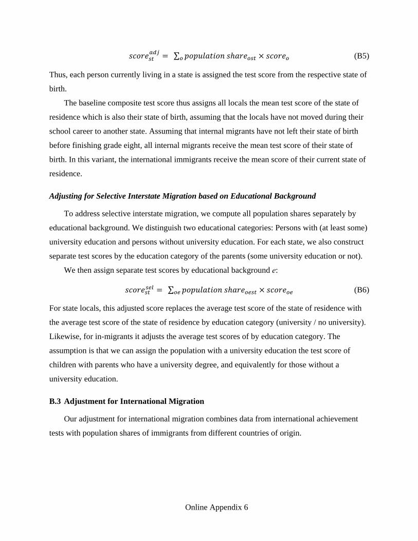
Online Appendix 6

𝑦𝑦𝑠𝑠𝑜𝑜𝑦𝑦𝑦𝑦𝑠𝑠𝑠𝑠𝑎𝑎𝑎𝑎𝑎𝑎 = ∑ 𝑝𝑝𝑜𝑜𝑝𝑝𝑝𝑝𝑜𝑜𝑦𝑦𝑝𝑝𝑜𝑜𝑜𝑜𝑜𝑜 𝑦𝑦ℎ𝑦𝑦𝑦𝑦𝑦𝑦𝑝𝑝𝑠𝑠𝑠𝑠 × 𝑦𝑦𝑠𝑠𝑜𝑜𝑦𝑦𝑦𝑦𝑝𝑝𝑝𝑝 (B5)

Thus, each person currently living in a state is assigned the test score from the respective state of

birth.

The baseline composite test score thus assigns all locals the mean test score of the state of

residence which is also their state of birth, assuming that the locals have not moved during their

school career to another state. Assuming that internal migrants have not left their state of birth

before finishing grade eight, all internal migrants receive the mean test score of their state of

birth. In this variant, the international immigrants receive the mean score of their current state of

residence.

Adjusting for Selective Interstate Migration based on Educational Background

To address selective interstate migration, we compute all population shares separately by

educational background. We distinguish two educational categories: Persons with (at least some)

university education and persons without university education. For each state, we also construct

separate test scores by the education category of the parents (some university education or not).

We then assign separate test scores by educational background e:

𝑦𝑦𝑠𝑠𝑜𝑜𝑦𝑦𝑦𝑦𝑠𝑠𝑠𝑠𝑠𝑠𝑝𝑝𝑠𝑠 = ∑ 𝑝𝑝𝑜𝑜𝑝𝑝𝑝𝑝𝑜𝑜𝑦𝑦𝑝𝑝𝑜𝑜𝑜𝑜𝑜𝑜 𝑦𝑦ℎ𝑦𝑦𝑦𝑦𝑦𝑦𝑝𝑝𝑝𝑝𝑠𝑠𝑠𝑠 × 𝑦𝑦𝑠𝑠𝑜𝑜𝑦𝑦𝑦𝑦𝑝𝑝𝑝𝑝𝑝𝑝𝑝𝑝 (B6)

For state locals, this adjusted score replaces the average test score of the state of residence with

the average test score of the state of residence by education category (university / no university).

Likewise, for in-migrants it adjusts the average test scores of by education category. The

assumption is that we can assign the population with a university education the test score of

children with parents who have a university degree, and equivalently for those without a

university education.

B.3 Adjustment for International Migration

Our adjustment for international migration combines data from international achievement

tests with population shares of immigrants from different countries of origin.

Online Appendix 7

International Test Score Data

We use international test score data from PISA, TIMSS, and PIRLS for international

immigrants residing in one of the U.S. states.3 As a first step, the international test data have to

be rescaled onto a common scale with the national NAEP data (Hanushek, Peterson, and

Woessmann (2012)). To do so, we first standardize all international test scores by subtracting

from each mean score on the international scale the U.S. mean value on the international scale by

subject, grade, and year and divide this difference by the U.S. standard deviation on the

international scale, also by subject, grade, and year. Next, we multiply the standardized value by

the U.S. standard deviation of the NAEP score by subject, grade, and year and add the U.S. mean

of the NAEP score by subject, grade, and year:

𝑦𝑦𝑠𝑠𝑜𝑜𝑦𝑦𝑦𝑦𝑠𝑠𝑒𝑒𝑠𝑠𝑠𝑠𝑎𝑎𝑎𝑎𝑎𝑎 = �

𝑠𝑠𝑠𝑠𝑝𝑝𝑝𝑝𝑝𝑝𝑖𝑖𝑠𝑠𝑠𝑠𝑖𝑖−𝑚𝑚𝑝𝑝𝑎𝑎𝑝𝑝𝑈𝑈𝑈𝑈,𝑠𝑠𝑠𝑠𝑖𝑖𝑖𝑖𝑖𝑖𝑖𝑖´𝑠𝑠

𝑠𝑠𝑎𝑎𝑈𝑈𝑈𝑈,𝑠𝑠𝑠𝑠𝑖𝑖𝑖𝑖𝑖𝑖𝑖𝑖´𝑠𝑠 � ∗ 𝑦𝑦𝑠𝑠𝑈𝑈𝑈𝑈,𝑒𝑒𝑠𝑠𝑠𝑠

𝑁𝑁𝑁𝑁𝑁𝑁𝑁𝑁 + 𝑚𝑚𝑦𝑦𝑦𝑦𝑜𝑜𝑈𝑈𝑈𝑈,𝑒𝑒𝑠𝑠𝑠𝑠𝑁𝑁𝑁𝑁𝑁𝑁𝑁𝑁 (B7)

where 𝑦𝑦𝑠𝑠𝑜𝑜𝑦𝑦𝑦𝑦𝑠𝑠𝑒𝑒𝑠𝑠𝑠𝑠 is the raw international test score of country s at grade g in subject u in year t.

To compute average test scores for each country, we proceed in the same way as for the

national test data. The regression design takes into account systematic differences between

grades, subjects, and years. The final estimate of the country average test score is then a country

fixed effect:

𝑦𝑦𝑠𝑠𝑜𝑜𝑦𝑦𝑦𝑦𝑠𝑠𝑒𝑒𝑠𝑠𝑠𝑠𝑠𝑠𝑠𝑠𝑎𝑎𝑝𝑝𝑎𝑎𝑎𝑎𝑝𝑝𝑎𝑎 = ∑ 𝛼𝛼𝑠𝑠𝐼𝐼𝑠𝑠𝑠𝑠 + 𝐼𝐼𝑒𝑒 ∗ 𝐼𝐼𝑠𝑠 ∗ 𝐼𝐼𝑠𝑠𝑝𝑝𝑠𝑠𝑠𝑠 + 𝐼𝐼𝑠𝑠 + 𝜖𝜖𝑠𝑠𝑒𝑒𝑠𝑠𝑠𝑠 (B8)

where 𝐼𝐼𝑠𝑠 is the fixed effect of country s that we are interested in. 𝐼𝐼𝑠𝑠 are time fixed effects and

𝐼𝐼𝑒𝑒 ∗ 𝐼𝐼𝑠𝑠 ∗ 𝐼𝐼𝑠𝑠𝑝𝑝𝑠𝑠𝑠𝑠 are grade times subject times survey fixed effects. The survey fixed effects indicate

whether we identify grade 4 in PIRLS or grade 4 in TIMSS. Thus, they are dummy variables for

TIMSS, PIRLS, and PISA. Again, the same regression can be estimated for different subsamples

of the population.4

3 We draw the data from the International Data Explorer (IDE) of the National Center of Education Statistics

(http://nces.ed.gov/surveys/international/ide/). 4 When estimating separate scores by the education category of the father, in PISA we use a simple average of

the test scores in ISCED categories 0-4 for non-university education and ISCED categories 5a and 6 for university education. In TIMSS 1995 and 1999, we use the average of the categories until “finished secondary” for non-university education and “finished university” for university education. In the subsequent TIMSS waves, we use ISCED categories 0-4 for non-university education and ISCED categories 5a and more than 5a for university education. The IDE does not report educational background variables for PIRLS and TIMSS grade 4.

Online Appendix 8

Apart from the mean test score, we also estimate the performance of the 75th and the 90th

percentile of students in each country for comparison. We also estimate the standard deviation.5

In cases where a source country did not participate in the international achievement tests, we

impute values from neighboring countries or regions. Table A5 reports the respective

imputations for the main source countries of immigrants in the United States.

Selectivity Adjustment of Home-Country Test Scores

As discussed in the paper, the skills of migrants are not random draws from the home-

country skill distribution. To estimate the migrant selectivity for each country, we proceed in two

steps. First, for each country of origin (country subscripts omitted), we calculate the selectivity

parameter for school attainment as the percentile p of the home-country distribution from which

the average immigrant to the U.S. is drawn:

𝑝𝑝 = 𝑦𝑦𝑈𝑈𝑈𝑈𝑝𝑝𝑝𝑝𝑒𝑒 ∗ 1

2𝑦𝑦ℎ𝑝𝑝𝑚𝑚𝑝𝑝𝑝𝑝𝑝𝑝𝑒𝑒 + 𝑦𝑦𝑈𝑈𝑈𝑈𝑠𝑠𝑝𝑝𝑠𝑠 ∗ �𝑦𝑦ℎ𝑝𝑝𝑚𝑚𝑝𝑝

𝑝𝑝𝑝𝑝𝑒𝑒 + 12𝑦𝑦ℎ𝑝𝑝𝑚𝑚𝑝𝑝𝑠𝑠𝑝𝑝𝑠𝑠 � + 𝑦𝑦𝑈𝑈𝑈𝑈𝑠𝑠𝑝𝑝𝑝𝑝 ∗ �𝑦𝑦ℎ𝑝𝑝𝑚𝑚𝑝𝑝

𝑝𝑝𝑝𝑝𝑒𝑒 + 𝑦𝑦ℎ𝑝𝑝𝑚𝑚𝑝𝑝𝑠𝑠𝑝𝑝𝑠𝑠 + 1

2𝑦𝑦ℎ𝑝𝑝𝑚𝑚𝑝𝑝𝑠𝑠𝑝𝑝𝑝𝑝 � (B9)

where the respective educational degrees of the population are given by pri = primary, sec =

secondary, and ter = tertiary, s refers to the shares of the population with the respective degrees

(with spri+ ssec+ ster=1), home refers to the population in the respective home country, and US

refers to the immigrants from the specific home country living in the United States. Data are

taken from Docquier, Lowell, and Marfouk (2009) and refer to the year 2000.

Second, to adjust for skill selectivity within educational degrees, our baseline estimate uses

the country-specific attainment selection parameter p to calculate the percentile of the cognitive

skill distribution for the average immigrant as 𝑝𝑝∗ = 𝑝𝑝 + 𝑝𝑝 ∗ (1 − 𝑝𝑝). For each country, we know

the mean and standard deviation of the test score distribution. Assuming a normal distribution,

we can calculate the corresponding test score that is adjusted for international migrant

selectivity:

𝑦𝑦𝑠𝑠𝑜𝑜𝑦𝑦𝑦𝑦𝑠𝑠𝑒𝑒𝑠𝑠𝑠𝑠𝑠𝑠𝑝𝑝𝑠𝑠𝑝𝑝𝑠𝑠𝑠𝑠𝑒𝑒𝑠𝑠𝑒𝑒𝑠𝑠𝑠𝑠 = 𝑜𝑜𝑜𝑜𝑖𝑖𝑜𝑜𝑜𝑜𝑦𝑦𝑚𝑚(𝑝𝑝∗) ∗ 𝑦𝑦𝑠𝑠𝑠𝑠𝑒𝑒𝑠𝑠𝑠𝑠𝑠𝑠𝑠𝑠𝑎𝑎𝑝𝑝𝑎𝑎𝑎𝑎𝑝𝑝𝑎𝑎 + 𝑦𝑦𝑠𝑠𝑜𝑜𝑦𝑦𝑦𝑦𝑠𝑠𝑒𝑒𝑠𝑠𝑠𝑠𝑠𝑠𝑠𝑠𝑎𝑎𝑝𝑝𝑎𝑎𝑎𝑎𝑝𝑝𝑎𝑎 (B10)

where 𝑜𝑜𝑜𝑜𝑖𝑖𝑜𝑜𝑜𝑜𝑦𝑦𝑚𝑚(𝑝𝑝∗) are draws of the p*th percentile from a normal (0,1) distribution,

𝑦𝑦𝑠𝑠𝑜𝑜𝑦𝑦𝑦𝑦𝑠𝑠𝑒𝑒𝑠𝑠𝑠𝑠𝑠𝑠𝑠𝑠𝑎𝑎𝑝𝑝𝑎𝑎𝑎𝑎𝑝𝑝𝑎𝑎 is the average international test score of country s at grade g in subject u in year t,

and 𝑦𝑦𝑠𝑠𝑠𝑠𝑒𝑒𝑠𝑠𝑠𝑠𝑠𝑠𝑠𝑠𝑎𝑎𝑝𝑝𝑎𝑎𝑎𝑎𝑝𝑝𝑎𝑎 is the corresponding standard deviation. The comparison of 𝑦𝑦𝑠𝑠𝑜𝑜𝑦𝑦𝑦𝑦𝑠𝑠𝑠𝑠𝑝𝑝𝑠𝑠𝑝𝑝𝑠𝑠𝑠𝑠𝑒𝑒𝑠𝑠𝑒𝑒𝑠𝑠𝑠𝑠 in

5 Standard deviations are again adjusted to be on the same scale with NAEP.

Online Appendix 9

math, grade 8, in the year 2007, using 𝑝𝑝∗ = 75 and 𝑝𝑝∗ = 90, respectively, with the available

country-specific observed test scores at the 75th and 90th percentile, respectively, show that this

prediction works well (correlations almost perfect with r = 99 percent in both cases). In further

analysis, we use 𝑝𝑝∗ = 𝑝𝑝 (according to equation (B9)) and 𝑝𝑝∗ = 90, respectively.

Population Shares of Immigrants from Different Countries of Origin

Using Census data, we next calculate the population shares of those born outside U.S. Table

A5 shows the main source countries of immigrants who came to the United States over the last

70 years.

In calculating the share of immigrants from different origin countries in the birthplace

composition of each state, we take into account the age of immigration. In particular, immigrants

arriving in the United States before the age of 6 are assumed to have spent their school career in

the U.S. school system, so they are assigned the NAEP score of their state of residence. Those

who immigrated after the age of 20 are assigned the test score of their country of origin. And

those who immigrated between ages 6 and 20 are assigned a weighted average of the two.

Using the population shares of immigrants from different countries of origin as in equation

(B4), we then basically proceed in the same way as with the national test score data. That is, we

adjust the composite test score of each state by applying the selectivity-adjusted country-of-

origin test scores for international immigrants.

B.4 Backward Projection of Time-Varying Scores

Finally, we employ two methods of age projections of historical achievement patterns, one

based on extrapolation from the available NAEP data and one based on projection from state

SAT scores.

Extrapolation of NAEP Trends

The skill measures developed so far assume that an average test score applies to the whole

working-age population. We now aim to project developments of cognitive skills over time by

state. Because test score data are not available before 1990 at the state level, we project test

scores back in time, incorporating the long-term national trend which dates back to 1978 for

eighth-grade math. For the projections, we do not use the 1990 value but rather start in 1992, as

the very first test scores seem to differ somewhat from the subsequent trends. The basic idea of

Online Appendix 10

our backward projection is to use an average of the linear trend in the state test score and the

observed national trend to predict the test score of the state in a given year until 1978, i.e. from

1978 to 1992.

The national NAEP series that goes back until 1978, called long-term trend NAEP, is on a

slightly different scale than the state NAEP series used in the state analysis. First, as scores

reported prior to 2004 are reported in a different testing format and both formats are reported for

2004, we align the prior scores by standardization equivalent to the adjustment for scores without

accommodation above. Then, to make the scales comparable, we subtract from each long-term

trend test score the long-term trend score in 1992 and divide by the U.S. standard deviation in

1992 from the long-term trend. We then multiply this term by the U.S. standard deviation in

1992 from the state NAEP series and add the national mean from the from the state NAEP series.

We start the projection by interpolating the available test scores linearly for each state from

1992 to 2011.6 The projection then follows an iterative process: We assume that each test score

of state s in t–1, 𝑇𝑇�𝑠𝑠,𝑠𝑠−1, is equal to the test score in t, 𝑇𝑇𝑠𝑠𝑠𝑠, minus a simple average of the change in

the state-specific linear time trend, i.e. the slope of the time trend, and the change in the national

time trend:

𝑇𝑇�𝑠𝑠,𝑠𝑠−1 = 𝑇𝑇𝑠𝑠𝑠𝑠 −12�𝑥𝑥𝑠𝑠𝛥𝛥𝛥𝛥𝑜𝑜𝑜𝑜𝑦𝑦𝑦𝑦𝑦𝑦 𝑆𝑆𝑝𝑝𝑦𝑦𝑝𝑝𝑦𝑦 𝑇𝑇𝑦𝑦𝑦𝑦𝑜𝑜𝑠𝑠𝑠𝑠𝑠𝑠 + 𝛥𝛥𝑁𝑁𝑦𝑦𝑝𝑝𝑁𝑁𝑜𝑜𝑜𝑜𝑦𝑦𝑜𝑜𝑠𝑠�������������� (B11)

where

𝛥𝛥𝛥𝛥𝑜𝑜𝑜𝑜𝑦𝑦𝑦𝑦𝑦𝑦 𝑆𝑆𝑝𝑝𝑦𝑦𝑝𝑝𝑦𝑦 𝑇𝑇𝑦𝑦𝑦𝑦𝑜𝑜𝑠𝑠𝑠𝑠𝑠𝑠 = 𝛥𝛥𝑜𝑜𝑜𝑜𝑦𝑦𝑦𝑦𝑦𝑦 𝑆𝑆𝑝𝑝𝑦𝑦𝑝𝑝𝑦𝑦 𝑇𝑇𝑦𝑦𝑦𝑦𝑜𝑜𝑠𝑠𝑠𝑠𝑠𝑠 − 𝛥𝛥𝑜𝑜𝑜𝑜𝑦𝑦𝑦𝑦𝑦𝑦 𝑆𝑆𝑝𝑝𝑦𝑦𝑝𝑝𝑦𝑦 𝑇𝑇𝑦𝑦𝑦𝑦𝑜𝑜𝑠𝑠𝑠𝑠,𝑠𝑠−1

𝛥𝛥𝑁𝑁𝑦𝑦𝑝𝑝𝑁𝑁𝑜𝑜𝑜𝑜𝑦𝑦𝑜𝑜𝑠𝑠������������� = 𝑁𝑁𝑦𝑦𝑝𝑝𝑁𝑁𝑜𝑜𝑜𝑜𝑦𝑦𝑜𝑜𝑠𝑠������������� − 𝑁𝑁𝑦𝑦𝑝𝑝𝑁𝑁𝑜𝑜𝑜𝑜𝑦𝑦𝑜𝑜𝑠𝑠−1����������������

The 𝛥𝛥𝑜𝑜𝑜𝑜𝑦𝑦𝑦𝑦𝑦𝑦 𝑆𝑆𝑝𝑝𝑦𝑦𝑝𝑝𝑦𝑦 𝑇𝑇𝑦𝑦𝑦𝑦𝑜𝑜𝑠𝑠𝑠𝑠𝑠𝑠 is obtained from state-specific regressions of the test score on years.

𝑁𝑁𝑦𝑦𝑝𝑝𝑁𝑁𝑜𝑜𝑜𝑜𝑦𝑦𝑜𝑜𝑠𝑠������������� is the long-term trend national average and available backwards until 1978.

To ensure that the (weighted) average of all state test scores is equal to the national average,

we adjust the linear state trend with a time-varying constant, 𝑥𝑥𝑠𝑠. This adjustment factor is

computed by taking the weighted sum of the test score projection on both sides and solving for

𝑥𝑥𝑠𝑠: 6 A few states started representative NAEP testing later than 1992. These are Alaska, Montana, Oregon,

Vermont, and Washington in 1996, Illinois, Kansas, and Nevada in 2000, and South Dakota in 2003. We project their scores back to 1992 with a simple backward projection method: 𝑇𝑇�𝑠𝑠,𝑠𝑠−1 = 𝑇𝑇𝑠𝑠𝑠𝑠 −

12�𝛥𝛥𝛥𝛥𝑜𝑜𝑜𝑜𝑦𝑦𝑦𝑦𝑦𝑦 𝑆𝑆𝑝𝑝𝑦𝑦𝑝𝑝𝑦𝑦 𝑇𝑇𝑦𝑦𝑦𝑦𝑜𝑜𝑠𝑠𝑠𝑠𝑠𝑠 +

𝛥𝛥𝑁𝑁𝑦𝑦𝑝𝑝𝑁𝑁𝑜𝑜𝑜𝑜𝑦𝑦𝑜𝑜𝑠𝑠��������������.

Online Appendix 11

𝑁𝑁𝑦𝑦𝑝𝑝𝑁𝑁𝑜𝑜𝑜𝑜𝑦𝑦𝑜𝑜𝑠𝑠−1���������������� = ∑ 𝑤𝑤𝑠𝑠𝑇𝑇�𝑠𝑠,𝑠𝑠−151𝑠𝑠=1 , 𝑜𝑜𝑜𝑜𝑦𝑦 𝑝𝑝 ≤ 1991 𝑦𝑦𝑜𝑜𝑠𝑠 ∑ 𝑤𝑤𝑠𝑠51

𝑠𝑠=1 = 1

⟺ 𝑥𝑥𝑠𝑠 = 2∗∑ 𝑤𝑤𝑖𝑖𝑇𝑇𝑖𝑖𝑖𝑖51𝑖𝑖=1 −𝑁𝑁𝑎𝑎𝑠𝑠𝑁𝑁𝑝𝑝𝑝𝑝𝑎𝑎𝑠𝑠𝑖𝑖���������������−𝑁𝑁𝑎𝑎𝑠𝑠𝑁𝑁𝑝𝑝𝑝𝑝𝑎𝑎𝑠𝑠𝑖𝑖−1������������������

∑ 𝑤𝑤𝑖𝑖𝛥𝛥𝛥𝛥𝑒𝑒𝑝𝑝𝑝𝑝𝑎𝑎𝑝𝑝 𝑈𝑈𝑠𝑠𝑎𝑎𝑠𝑠𝑝𝑝 𝑇𝑇𝑝𝑝𝑝𝑝𝑝𝑝𝑎𝑎𝑖𝑖𝑖𝑖51𝑖𝑖=1

(B12)

The weights, 𝑤𝑤𝑠𝑠, are based on average daily attendance in public elementary and secondary

schools by state from the Digest of Education Statistics (U.S. Department of Education (2013)).

To obtain a weight for each state, we divide the average daily attendance in the state by the total

national daily attendance. This measure is averaged over the time period 1978 to 1992 as the

fractions are rather stable. The cross-sectional correlation between the fractions in 1978 and in

1992 is 98 percent.

This part of the extrapolation is exemplified by Figure A2, which shows both the observed

data and the extrapolated state trends for two states: Massachusetts and Mississippi.

Massachusetts was above the national average in 2011, but also had a steeper growth trend than

the nation as a whole. As such, we shrink the extrapolated trend toward the national trend.

Mississippi is different: while it also had a steeper growth trend than the nation as a whole, its

scores were below the national average. Again, we shrink the extrapolation to the nationally

observed trend.

The projected test score series then uses the available test score information for each state

from 1992 to 2011 and the projected scores from the above iterative procedure from 1978 to

1992. Before 1978, we either assume a constant test score or a linear state trend.

The adjusted skill measure is then constructed by taking five-year averages of the projected

test score series. These five year averages are then matched to the population shares of the

appropriate age. To match the projected test score data, the share of people from origin o living

in state s in equation (B4) is computed in five-year age intervals from the Census data, both for

the state average and for the education-category subsamples. The adjusted skill measure is then

derived as

𝑦𝑦𝑠𝑠𝑜𝑜𝑦𝑦𝑦𝑦𝑠𝑠𝑠𝑠𝑝𝑝𝑝𝑝𝑝𝑝𝑎𝑎𝑝𝑝𝑠𝑠𝑠𝑠𝑝𝑝𝑎𝑎 = ∑ 𝑝𝑝𝑜𝑜𝑝𝑝𝑝𝑝𝑜𝑜𝑦𝑦𝑝𝑝𝑜𝑜𝑜𝑜𝑜𝑜 𝑦𝑦ℎ𝑦𝑦𝑦𝑦𝑦𝑦𝑝𝑝𝑝𝑝𝑎𝑎𝑠𝑠𝑠𝑠 × 𝑦𝑦𝑠𝑠𝑜𝑜𝑦𝑦𝑦𝑦𝑝𝑝𝑝𝑝𝑎𝑎𝑝𝑝𝑝𝑝𝑎𝑎 (B13)

where the population shares and scores now do not only vary by state of origin o and educational

category e, but also by age category a.

Online Appendix 12

Projection from State SAT Scores

We obtained state-specific SAT scores (in math, writing, and reading) from 1972 to 2013

from the College Board. SAT scores are not representative for the total student population. But

College Board also provided information on total participation (number of test takers). We

calculate SAT participation rates by dividing the number of SAT participants by the total number

of public high school graduates in each state. The latter is collected from various years of the

Digest of Education Statistics (filling gaps by linear interpolation between available years).

Regressing the SAT score on the participation rate shows a significant negative relationship,

indicating that a higher participation rate is related to a less selective sample and lower test

scores. We therefore construct a series of participation-adjusted SAT scores:

𝑆𝑆𝑆𝑆𝑇𝑇 𝑦𝑦𝑠𝑠𝑜𝑜𝑦𝑦𝑦𝑦𝑠𝑠𝑠𝑠 = 𝛼𝛼0 + 𝛼𝛼1𝑝𝑝𝑦𝑦𝑦𝑦𝑝𝑝𝑜𝑜𝑠𝑠𝑜𝑜𝑝𝑝𝑦𝑦𝑝𝑝𝑜𝑜𝑜𝑜𝑜𝑜 𝑦𝑦𝑦𝑦𝑝𝑝𝑦𝑦𝑠𝑠𝑠𝑠 + 𝜆𝜆𝑠𝑠 + 𝜆𝜆𝑠𝑠 + 𝜖𝜖𝑠𝑠𝑠𝑠 (B14)

We use the estimated coefficients to predict SAT test scores with constant participation

rates, where we assume that all states have the mean U.S. participation rate over the period 1972

to 2013 of 46.9 percent.

The participation-adjusted SAT scores allow us to predict state NAEP scores before 1992.

To do so, we first regress the eighth-grade math test scores in NAEP on the participation-

adjusted SAT scores by state for the years since 1992 where both test scores series are available:

𝑁𝑁𝑆𝑆𝑁𝑁𝑁𝑁 𝑦𝑦𝑠𝑠𝑜𝑜𝑦𝑦𝑦𝑦𝑠𝑠 = 𝛽𝛽0 + 𝛽𝛽1𝑆𝑆𝑆𝑆𝑇𝑇 𝑦𝑦𝑠𝑠𝑜𝑜𝑦𝑦𝑦𝑦𝑠𝑠𝑎𝑎𝑎𝑎𝑎𝑎𝑠𝑠𝑠𝑠𝑠𝑠𝑝𝑝𝑎𝑎 + 𝜖𝜖𝑠𝑠 (B15)

Because the SAT is taken around high school graduation, in these regressions we lag the

SAT test scores by four years to capture almost the same cohorts as in NAEP. The regressions

show that the participation-adjusted SAT score and the NAEP score move together over time in

almost all states.7

With the estimated coefficients, we can then construct predicted NAEP test scores for each

state for the years 1968 to 1991. Applying the same algorithm for the projection of test scores by

age as before, we construct new aggregate test scores for each state and year by using the

predicted NAEP test scores based on the SAT data.

7 Exceptions are Kansas, Nevada, and South Dakota, which are also the states that start relatively late in

NAEP, thereby impeding the prediction of a reliable connection between NAEP and SAT. For these states, we use the U.S. average coefficient.

Online Appendix 13

Additional Appendix Tables

Table A2: Selectivity of Migrant Sending Countries Country School-attainment selectivity Country School-attainment selectivity Adjusted Unadjusted Adjusted Unadjusted Mongolia 0.997 0.948 England 0.938 0.752 Indonesia 0.989 0.894 Scotland 0.938 0.752 Macedonia 0.988 0.893 United Kingdom 0.938 0.752 Botswana 0.987 0.887 American Samoa 0.936 0.746 Ghana 0.985 0.877 Guam 0.936 0.746 Southern Africa 0.985 0.878 Japan 0.936 0.747 Africa 0.984 0.872 Overseas Territories 0.936 0.746 Algeria 0.984 0.872 U.S. Virgin Islands 0.936 0.746 Morocco 0.983 0.869 Israel/Palestine 0.934 0.751 South Africa 0.983 0.870 Kazakhstan 0.933 0.742 Egypt 0.982 0.867 Panama 0.933 0.741 Northern Africa 0.982 0.867 Colombia 0.932 0.738 Tunisia 0.981 0.861 Estonia 0.932 0.739 Bahrain 0.978 0.852 Baltic States 0.931 0.738 Iran 0.978 0.853 Denmark 0.931 0.737 Qatar 0.978 0.853 New Zealand 0.930 0.736 Saudi Arabia 0.978 0.852 Trinidad and Tobago 0.930 0.736 United Arab Emirates 0.978 0.853 Sweden 0.929 0.733 Singapore 0.977 0.850 Western Europe 0.929 0.741 Kuwait 0.974 0.839 Belgium 0.928 0.731 Liechtenstein 0.974 0.838 Former USSR without Russia 0.928 0.734 Switzerland 0.972 0.833 Chile 0.927 0.730 Taiwan (Chinese Taipei) 0.970 0.827 Former USSR 0.927 0.731 Southeast Asia + Iran 0.968 0.825 Kyrgyzstan 0.927 0.729 Brazil 0.966 0.816 Hungary 0.926 0.728 Turkey 0.966 0.817 Finland 0.925 0.725 Southeast Asia 0.965 0.820 South America 0.925 0.730 Palestinian Nat'l Auth. 0.963 0.809 Total Average 0.925 0.744 Thailand 0.962 0.806 Netherlands 0.923 0.723 Malaysia 0.956 0.790 Argentina 0.922 0.721 Asia 0.955 0.798 Lithuania 0.921 0.719 Middle East 0.955 0.798 Northern Europe 0.921 0.720 France 0.954 0.785 Ukraine 0.919 0.716 Georgia 0.953 0.784 Moldova 0.918 0.714 East Asia 0.950 0.791 Oceania 0.918 0.715 Lebanon 0.949 0.775 Syrian Arab Republic 0.918 0.713 Hong Kong 0.947 0.769 Europe 0.914 0.714 Macao-China 0.947 0.769 Iceland 0.914 0.708 Azerbaijan 0.944 0.763 Jordan 0.914 0.707 Spain 0.944 0.764 Antarctica 0.913 0.706 Philippines 0.943 0.760 Austria 0.912 0.704 Latvia 0.941 0.758 Montenegro 0.912 0.704 Bulgaria 0.938 0.750 Serbia 0.912 0.704

(continued on next page)

Online Appendix 14

Table A2 (continued) Country School-attainment selectivity Country School-attainment selectivity Adjusted Unadjusted Adjusted Unadjusted Slovak Rep. 0.912 0.703 Norway 0.894 0.674 Czechoslovakia 0.909 0.698 Central America 0.891 0.677 Romania 0.909 0.699 Bosnia and Herzegovina 0.889 0.666 Eastern Europe 0.907 0.698 Malta 0.885 0.660 Australia 0.906 0.693 Poland 0.885 0.661 Czech Rep. 0.906 0.693 Croatia 0.884 0.66 Yugoslavia 0.906 0.707 Ireland 0.879 0.652 Cyprus 0.905 0.692 Honduras 0.876 0.647 Oman 0.905 0.692 Germany 0.872 0.643 Peru 0.905 0.692 Portugal 0.865 0.633 Armenia 0.903 0.688 Italy 0.863 0.629 Korea, Rep. 0.902 0.688 Greece 0.850 0.613 Albania 0.901 0.685 El Salvador 0.827 0.584 Southern Europe 0.899 0.697 Canada 0.774 0.525 Uruguay 0.898 0.681 North America 0.774 0.525 Luxembourg 0.894 0.674 Mexico 0.710 0.461

Notes: Selectivity of U.S. immigrants based on their home-country distribution of school attainment. See section 2.3.3 for details.

Online Appendix 15

Table A3: Summary Statistics

Obs. Mean Std. dev. Min. Max.

Real GDP per capita, 2007 47 41,218 6,388 29,302 59,251

Years of schooling, 2007 47 13.11 0.35 12.52 13.74

Test scores:

Baseline: local average adjusted for interstate migrants 47 499.9 15.98 460.4 527.7

+ Adjustment of locals by education category 47 494.4 15.46 454.9 521.3

+ Adjustment of interstate migrants by education category 47 493.9 15.80 453.1 522.0

+ Adjustment of international migrants scores by selectivity 47 497.7 15.57 454.8 524.7

Age adjustment with extrapolation of NAEP trends by education category 47 442.4 22.04 381.9 476.5

Age adjustment with projection from SAT scores 47 407.2 27.52 321.5 456.6

Growth rate of real GDP per capita, 1970-2007 47 2.24 0.31 1.56 2.89

Change in years of schooling, 1970-2007 47 2.02 0.45 0.78 2.86

Estimated annual change in test scores, 1968-2011 47 3.17 1.21 1.17 6.77

Notes: See sections 2.2, 2.3, and 3.1 for details on the data. Test scores refer to eighth-grade math. Locals are all persons who report a state of birth equal to the current state of residence. Interstate migrants report another state of birth than state of residence. International migrants report another country of birth than the United States. “By education category” indicates that individuals with/without university education are assigned the test scores of children of parents with/without university education.

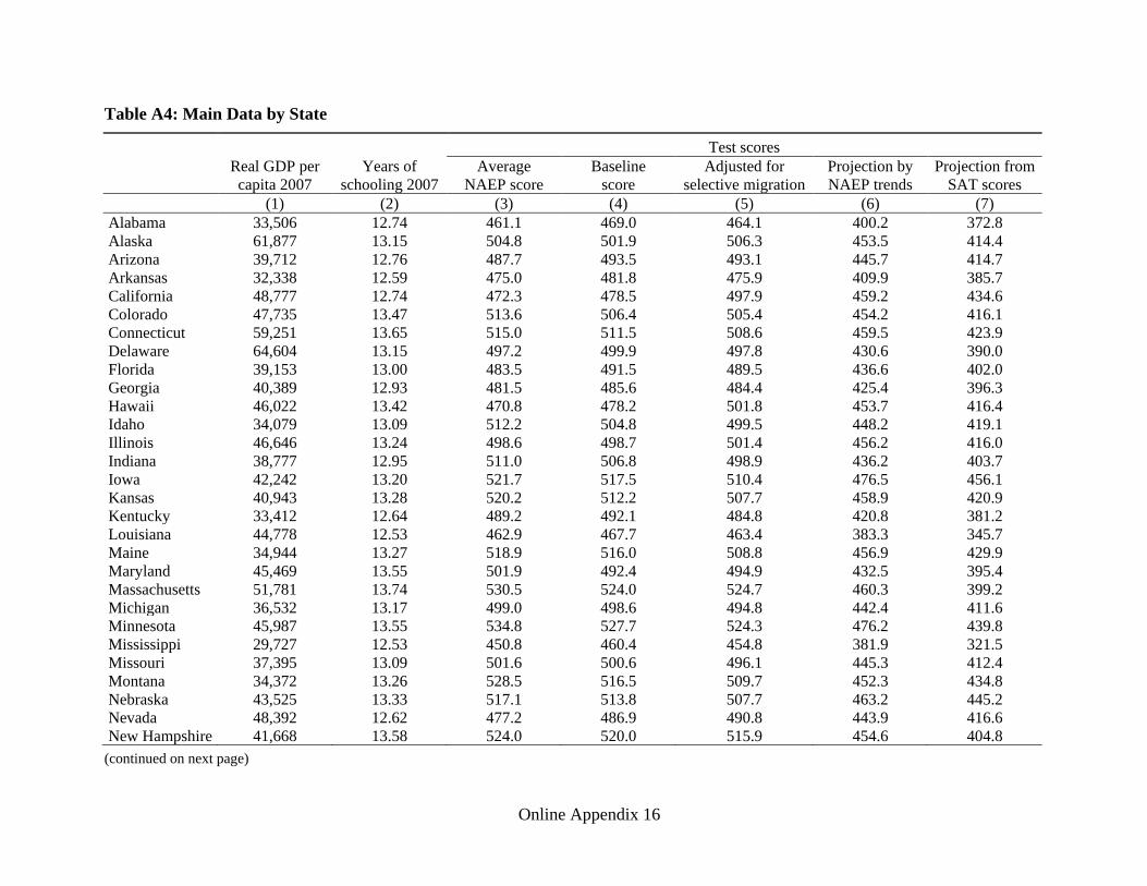
Online Appendix 16

Table A4: Main Data by State

Test scores Real GDP per

capita 2007 Years of

schooling 2007 Average

NAEP score Baseline

score Adjusted for

selective migration Projection by NAEP trends

Projection from SAT scores

(1) (2) (3) (4) (5) (6) (7) Alabama 33,506 12.74 461.1 469.0 464.1 400.2 372.8 Alaska 61,877 13.15 504.8 501.9 506.3 453.5 414.4 Arizona 39,712 12.76 487.7 493.5 493.1 445.7 414.7 Arkansas 32,338 12.59 475.0 481.8 475.9 409.9 385.7 California 48,777 12.74 472.3 478.5 497.9 459.2 434.6 Colorado 47,735 13.47 513.6 506.4 505.4 454.2 416.1 Connecticut 59,251 13.65 515.0 511.5 508.6 459.5 423.9 Delaware 64,604 13.15 497.2 499.9 497.8 430.6 390.0 Florida 39,153 13.00 483.5 491.5 489.5 436.6 402.0 Georgia 40,389 12.93 481.5 485.6 484.4 425.4 396.3 Hawaii 46,022 13.42 470.8 478.2 501.8 453.7 416.4 Idaho 34,079 13.09 512.2 504.8 499.5 448.2 419.1 Illinois 46,646 13.24 498.6 498.7 501.4 456.2 416.0 Indiana 38,777 12.95 511.0 506.8 498.9 436.2 403.7 Iowa 42,242 13.20 521.7 517.5 510.4 476.5 456.1 Kansas 40,943 13.28 520.2 512.2 507.7 458.9 420.9 Kentucky 33,412 12.64 489.2 492.1 484.8 420.8 381.2 Louisiana 44,778 12.53 462.9 467.7 463.4 383.3 345.7 Maine 34,944 13.27 518.9 516.0 508.8 456.9 429.9 Maryland 45,469 13.55 501.9 492.4 494.9 432.5 395.4 Massachusetts 51,781 13.74 530.5 524.0 524.7 460.3 399.2 Michigan 36,532 13.17 499.0 498.6 494.8 442.4 411.6 Minnesota 45,987 13.55 534.8 527.7 524.3 476.2 439.8 Mississippi 29,727 12.53 450.8 460.4 454.8 381.9 321.5 Missouri 37,395 13.09 501.6 500.6 496.1 445.3 412.4 Montana 34,372 13.26 528.5 516.5 509.7 452.3 434.8 Nebraska 43,525 13.33 517.1 513.8 507.7 463.2 445.2 Nevada 48,392 12.62 477.2 486.9 490.8 443.9 416.6 New Hampshire 41,668 13.58 524.0 520.0 515.9 454.6 404.8

(continued on next page)

Online Appendix 17

Table A4 (continued)

Test scores Real GDP per

capita 2007 Years of

schooling 2007 Average

NAEP score Baseline

score Adjusted for

selective migration Projection by NAEP trends

Projection from SAT scores

(1) (2) (3) (4) (5) (6) (7) New Jersey 51,337 13.48 519.0 513.9 516.5 465.5 433.2 New Mexico 35,313 12.71 468.2 480.9 480.0 428.4 403.3 New York 53,165 13.27 497.8 498.4 508.8 460.1 426.4 North Carolina 41,123 12.98 497.3 497.1 492.3 416.1 358.3 North Dakota 41,329 13.47 531.8 527.0 520.3 472.8 456.6 Ohio 38,389 13.13 510.2 506.8 500.8 432.5 394.4 Oklahoma 36,504 12.84 488.5 491.4 486.2 437.8 412.4 Oregon 42,422 13.18 511.0 503.1 503.9 450.7 420.1 Pennsylvania 39,951 13.21 509.2 507.7 501.5 444.3 406.7 Rhode Island 42,274 13.05 489.4 495.8 495.5 445.4 411.0 South Carolina 33,539 12.85 490.5 492.7 486.8 414.8 354.5 South Dakota 41,649 13.12 521.6 518.6 508.7 460.5 427.1 Tennessee 37,068 12.74 475.8 482.1 477.3 415.5 374.3 Texas 45,502 12.52 502.7 499.8 496.8 438.1 400.2 Utah 39,464 13.26 506.5 502.9 497.2 454.7 434.7 Vermont 36,445 13.63 525.2 517.1 511.7 447.5 400.1 Virginia 47,501 13.44 508.3 501.8 501.6 441.0 402.6 Washington 47,553 13.37 513.8 506.8 514.2 460.2 391.5 West Virginia 29,302 12.53 475.7 483.0 472.8 411.9 380.2 Wisconsin 39,841 13.28 521.1 516.5 509.5 463.1 433.3 Wyoming 59,558 13.22 514.1 509.4 504.9 452.2 423.6

Notes: (1) Real GDP per capita in 2005 U.S. dollars. (2) Mean years of completed schooling, 2007. (3) Estimated average eighth-grade math NAEP score from 1992 to 2011, obtained from a regression of NAEP test scores on time and state fixed effects; see Appendix B.1. (4) Baseline: local average adjusted for interstate migrants by average test score of their state of birth. (5) Baseline + adjustment of locals by education category + adjustment of interstate migrants by education category + adjustment of international migrants by selectivity. (6) Age adjustment with extrapolation of NAEP trends by education category; see Appendix B.4. (7) Age adjustment with projection from SAT scores; see Appendix B.4.

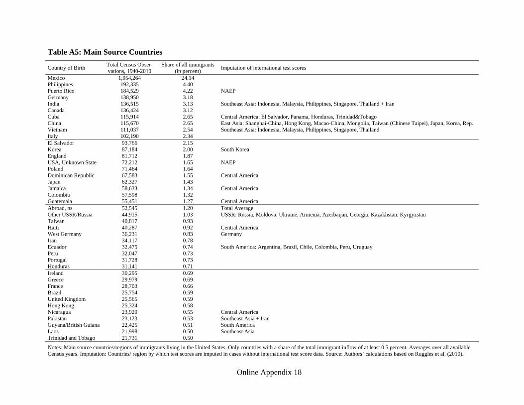
Online Appendix 18

Table A5: Main Source Countries

Country of Birth Total Census Obser-vations, 1940-2010

Share of all immigrants (in percent) Imputation of international test scores

Mexico 1,054,264 24.14 Philippines 192,335 4.40 Puerto Rico 184,529 4.22 NAEP Germany 138,950 3.18 India 136,515 3.13 Southeast Asia: Indonesia, Malaysia, Philippines, Singapore, Thailand + Iran Canada 136,424 3.12 Cuba 115,914 2.65 Central America: El Salvador, Panama, Honduras, Trinidad&Tobago China 115,670 2.65 East Asia: Shanghai-China, Hong Kong, Macao-China, Mongolia, Taiwan (Chinese Taipei), Japan, Korea, Rep. Vietnam 111,037 2.54 Southeast Asia: Indonesia, Malaysia, Philippines, Singapore, Thailand Italy 102,190 2.34 El Salvador 93,766 2.15 Korea 87,184 2.00 South Korea England 81,712 1.87 USA, Unknown State 72,212 1.65 NAEP Poland 71,464 1.64 Dominican Republic 67,583 1.55 Central America Japan 62,327 1.43 Jamaica 58,633 1.34 Central America Colombia 57,598 1.32 Guatemala 55,451 1.27 Central America Abroad, ns 52,545 1.20 Total Average Other USSR/Russia 44,915 1.03 USSR: Russia, Moldova, Ukraine, Armenia, Azerbaijan, Georgia, Kazakhstan, Kyrgyzstan Taiwan 40,817 0.93 Haiti 40,287 0.92 Central America West Germany 36,231 0.83 Germany Iran 34,117 0.78 Ecuador 32,475 0.74 South America: Argentina, Brazil, Chile, Colombia, Peru, Uruguay Peru 32,047 0.73 Portugal 31,728 0.73 Honduras 31,141 0.71 Ireland 30,295 0.69 Greece 29,979 0.69 France 28,703 0.66 Brazil 25,754 0.59 United Kingdom 25,565 0.59 Hong Kong 25,324 0.58 Nicaragua 23,920 0.55 Central America Pakistan 23,123 0.53 Southeast Asia + Iran Guyana/British Guiana 22,425 0.51 South America Laos 21,998 0.50 Southeast Asia Trinidad and Tobago 21,731 0.50

Notes: Main source countries/regions of immigrants living in the United States. Only countries with a share of the total immigrant inflow of at least 0.5 percent. Averages over all available Census years. Imputation: Countries/ region by which test scores are imputed in cases without international test score data. Source: Authors’ calculations based on Ruggles et al. (2010).

Online Appendix 19

Table A6: Development Accounting Results for Different Years

Test score specification Year Total knowledge capital Test scores Years of schooling Baseline: local average adjusted for interstate migrants 2007 0.150*** (0.045) 0.057** (0.025) 0.093*** (0.023)

2000 0.149*** (0.047) 0.061** (0.026) 0.088*** (0.024) 1990 0.127*** (0.048) 0.031 (0.029) 0.096*** (0.023) 1980 0.155** (0.078) 0.024 (0.038) 0.131*** (0.044) 1970 0.179*** (0.060) 0.028 (0.033) 0.151*** (0.032)

+ Adjustment of locals by education category 2007 0.159*** (0.043) 0.066*** (0.024) 0.093*** (0.023) 2000 0.157*** (0.046) 0.069*** (0.025) 0.088*** (0.024) 1990 0.138*** (0.046) 0.042 (0.027) 0.096*** (0.023) 1980 0.181** (0.076) 0.050 (0.035) 0.131*** (0.044) 1970 0.198*** (0.059) 0.047 (0.031) 0.151*** (0.032)

+ Adjustment of interstate migrants by education category 2007 0.169*** (0.043) 0.076*** (0.024) 0.093*** (0.023) 2000 0.165*** (0.047) 0.077*** (0.025) 0.088*** (0.024) 1990 0.145*** (0.046) 0.049* (0.026) 0.096*** (0.023) 1980 0.178** (0.075) 0.047 (0.034) 0.131*** (0.044) 1970 0.186*** (0.057) 0.035 (0.029) 0.151*** (0.032)

+ Adjustment of international migrants by selectivity 2007 0.190*** (0.041) 0.097*** (0.022) 0.093*** (0.023) 2000 0.180*** (0.045) 0.092*** (0.024) 0.088*** (0.024) 1990 0.169*** (0.043) 0.073*** (0.023) 0.096*** (0.023) 1980 0.195** (0.076) 0.064* (0.034) 0.131*** (0.044) 1970 0.203*** (0.056) 0.052* (0.028) 0.151*** (0.032)

Notes: Development accounting results (covariance measure) for 47 U.S. states with different test score specifications. Test scores refer to eighth-grade math. Locals are all persons who report a state of birth equal to the current state of residence. Interstate migrants report another state of birth than state of residence. International migrants report another country of birth than the United States. “By education category” indicates that individuals with/without university education are assigned the test scores of children of parents with/without university education. Calculations assume a return of w=0.17 per standard deviation in test scores and a return of r=0.08 per year of schooling. Bootstrapped standard errors in parentheses with 1,000 replications. Significance levels: * p < 0.10, ** p < 0.05, *** p < 0.01.

Online Appendix 20

Table A7: Five-State Measure: Alternative Numbers of Top and Bottom States

Total knowledge capital Test scores Years of schooling

Five-state measure 0.306 0.186 0.120 Three-state measure 0.307 0.170 0.137 Seven-state measure 0.261 0.164 0.097

Notes: Development accounting results (five-state measure) for 47 U.S. states with different numbers of countries used at the top and bottom of the state distribution. Test score specification adjusts locals and interstate migrants by age-education category based on extrapolation of NAEP trends by education category and international migrants by selectivity. Test scores refer to eighth-grade math. Calculations assume a return of w=0.17 per standard deviation in test scores and a return of r=0.08 per year of schooling.

Online Appendix 21

Table A8: Growth Accounting by State, 1970-2007

Average annual growth rate of

Absolute change in Estimated

Average annual growth rate accounted for by Percent of total growth

real GDP per

capita (percent) years of

schooling annual change in test scores

Total know-ledge capital

Test scores

Years of schooling Total know-

ledge capital Test

scores Years of schooling

(1) (2) (3) (4) (5) (6) (7) (8) (9) Alabama 2.35 2.65 2.77 0.70 0.31 0.38 29.6 13.4 16.3 Arizona 2.03 1.60 2.71 0.54 0.31 0.23 26.5 15.1 11.4 Arkansas 2.39 2.50 2.85 0.68 0.32 0.36 28.5 13.5 15.0 California 2.14 1.01 2.22 0.40 0.25 0.15 18.5 11.8 6.8 Colorado 2.58 1.57 3.38 0.61 0.38 0.23 23.6 14.8 8.8 Connecticut 2.79 2.25 2.77 0.64 0.31 0.32 22.9 11.3 11.6 Florida 2.16 1.98 3.93 0.73 0.45 0.29 33.9 20.6 13.2 Georgia 2.44 2.66 2.90 0.71 0.33 0.38 29.2 13.5 15.7 Hawaii 1.63 1.96 3.28 0.65 0.37 0.28 40.2 22.9 17.4 Idaho 2.02 1.53 2.08 0.46 0.24 0.22 22.6 11.7 10.9 Illinois 2.03 2.03 3.36 0.67 0.38 0.29 33.1 18.7 14.4 Indiana 2.01 1.85 3.28 0.64 0.37 0.27 31.8 18.5 13.3 Iowa 2.32 1.64 1.17 0.37 0.13 0.24 15.9 5.7 10.2 Kansas 2.43 1.63 3.10 0.59 0.35 0.23 24.1 14.4 9.6 Kentucky 1.86 2.62 3.64 0.79 0.41 0.38 42.6 22.2 20.3 Louisiana 2.41 2.33 4.30 0.82 0.49 0.34 34.2 20.3 14.0 Maine 2.20 2.20 1.63 0.50 0.18 0.32 22.8 8.4 14.4 Maryland 2.41 2.32 3.94 0.78 0.45 0.33 32.5 18.6 13.9 Massachusetts 2.56 2.21 5.47 0.94 0.62 0.32 36.7 24.2 12.5 Michigan 1.56 1.97 2.74 0.59 0.31 0.28 38.1 19.9 18.2 Minnesota 2.37 1.96 2.88 0.61 0.33 0.28 25.6 13.7 11.9 Mississippi 2.36 2.46 5.16 0.94 0.58 0.35 39.7 24.8 15.0 Missouri 1.89 2.10 2.56 0.59 0.29 0.30 31.3 15.3 16.0 Montana 2.10 1.68 1.42 0.40 0.16 0.24 19.2 7.7 11.5 Nebraska 2.42 1.67 1.54 0.42 0.17 0.24 17.1 7.2 10.0 Nevada 1.69 0.78 3.12 0.47 0.35 0.11 27.6 21.0 6.7 New Hampshire 2.56 2.16 2.85 0.64 0.32 0.31 24.8 12.6 12.2 New Jersey 2.41 2.25 3.41 0.71 0.39 0.32 29.5 16.1 13.5 (continued on next page)

Online Appendix 22

Table A8 (continued)

Average annual growth rate of

Absolute change in Estimated

Average annual growth rate accounted for by Percent of total growth

real GDP per

capita (percent) years of

schooling annual change in test scores

Total know-ledge capital

Test scores

Years of schooling Total know-

ledge capital Test

scores Years of schooling

(1) (2) (3) (4) (5) (6) (7) (8) (9) New Mexico 2.01 1.71 1.86 0.46 0.21 0.25 22.7 10.5 12.3 New York 2.12 2.05 3.49 0.69 0.40 0.30 32.6 18.7 13.9 North Carolina 2.30 2.76 6.06 1.08 0.69 0.40 47.2 29.9 17.3 North Dakota 2.86 2.38 1.46 0.51 0.17 0.34 17.7 5.8 12.0 Ohio 1.80 1.92 3.86 0.71 0.44 0.28 39.7 24.3 15.4 Oklahoma 2.26 1.71 1.93 0.47 0.22 0.25 20.6 9.7 10.9 Oregon 2.31 1.58 2.13 0.47 0.24 0.23 20.3 10.4 9.8 Pennsylvania 2.04 2.20 3.24 0.68 0.37 0.32 33.5 18.0 15.5 Rhode Island 2.32 2.19 2.67 0.62 0.30 0.32 26.6 13.1 13.6 South Carolina 2.30 2.86 5.35 1.02 0.61 0.41 44.2 26.4 17.9 South Dakota 2.89 1.89 2.94 0.61 0.33 0.27 20.9 11.5 9.4 Tennessee 2.29 2.52 3.59 0.77 0.41 0.36 33.7 17.8 15.9 Texas 2.48 1.85 4.43 0.77 0.50 0.27 30.9 20.2 10.7 Utah 2.41 1.22 1.93 0.39 0.22 0.18 16.4 9.1 7.3 Vermont 2.00 2.19 4.02 0.77 0.46 0.32 38.5 22.8 15.8 Virginia 2.69 2.66 3.74 0.81 0.42 0.38 30.0 15.8 14.3 Washington 2.24 1.48 6.77 0.98 0.77 0.21 43.8 34.3 9.5 West Virginia 1.67 2.33 2.88 0.66 0.33 0.34 39.6 19.5 20.1 Wisconsin 2.17 1.94 2.26 0.54 0.26 0.28 24.7 11.8 12.9 Notes: Estimated annual change in test scores: in percent of a standard deviation, obtained from a regression of test scores (NAEP scores projected based on participation-corrected SAT scores as derived in section 2.3.4) on years for each state, 1968-2011.

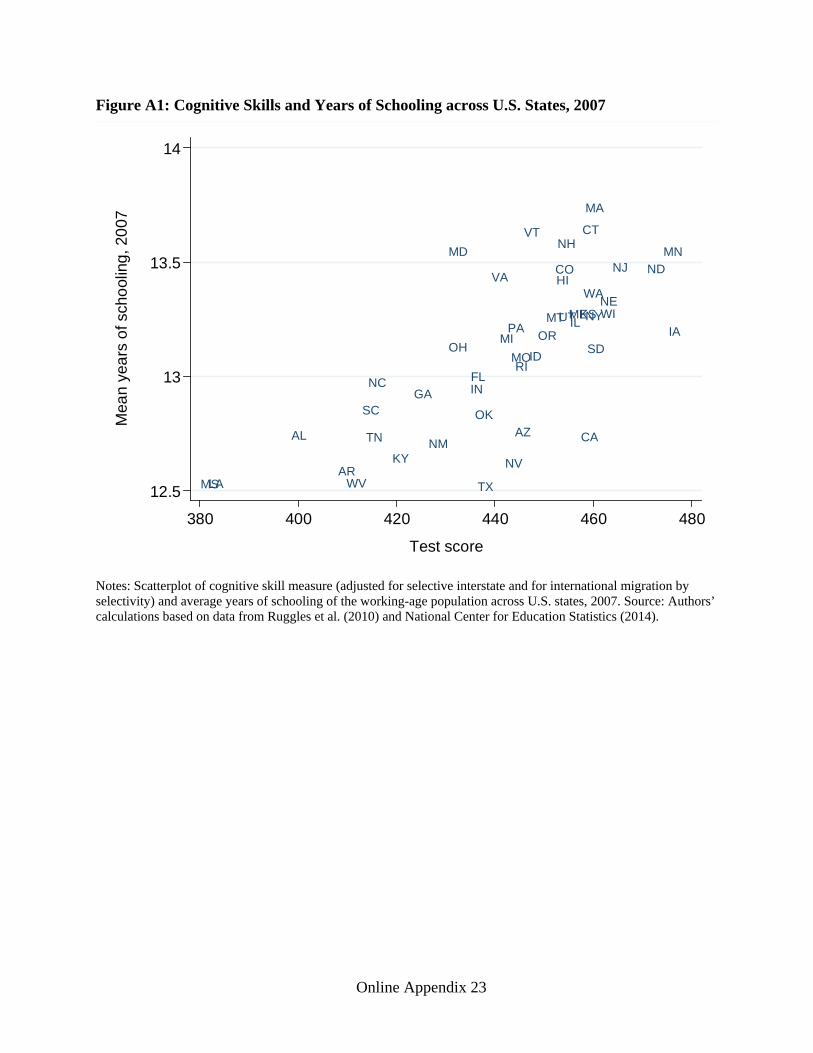
Online Appendix 23

Figure A1: Cognitive Skills and Years of Schooling across U.S. States, 2007

AL AZ

AR

CA

CO

CT

FLGA

HI

ID

IL

IN

IAKS

KY

LA

ME

MD

MA

MI

MN

MS

MO

MTNE

NV

NH

NJ

NM

NY

NC

ND

OH

OK

ORPA

RI

SC

SD

TN

TX

UT

VT

VAWA

WV

WI

12.5

13

13.5

14

Mea

n ye

ars

of s

choo

ling,

200

7

380 400 420 440 460 480

Test score

Notes: Scatterplot of cognitive skill measure (adjusted for selective interstate and for international migration by selectivity) and average years of schooling of the working-age population across U.S. states, 2007. Source: Authors’ calculations based on data from Ruggles et al. (2010) and National Center for Education Statistics (2014).

Online Appendix 24

Figure A2: Projection of Test Scores for Massachusetts and Mississippi

Notes: NAEP test score in eighth-grade math. Source: Authors’ calculations based on data from National Center for Education Statistics (2014).

350

400

450

500

550

1980 1990 2000 2010 1980 1990 2000 2010

Massachusetts Mississippi

State Trend Linear State TrendNational Trend Extrapolated State Trend

Stan

dard

ized

test

sco

re

Year