Kernel Belief Propagation

707

Kernel Belief Propagation

Le Song,1 Arthur Gretton,1,2 Danny Bickson,1 Yucheng Low,1 Carlos Guestrin1

1 School of Computer Science, CMU; 2Gatsby Computational Neuroscience Unit & MPI for Biological Cybernetics

Abstract

We propose a nonparametric generalization ofbelief propagation, Kernel Belief Propagation(KBP), for pairwise Markov random fields. Mes-sages are represented as functions in a repro-ducing kernel Hilbert space (RKHS), and mes-sage updates are simple linear operations in theRKHS. KBP makes none of the assumptionscommonly required in classical BP algorithms:the variables need not arise from a finite do-main or a Gaussian distribution, nor must theirrelations take any particular parametric form.Rather, the relations between variables are rep-resented implicitly, and are learned nonparamet-rically from training data. KBP has the advan-tage that it may be used on any domain wherekernels are defined (Rd, strings, groups), evenwhere explicit parametric models are not known,or closed form expressions for the BP updatesdo not exist. The computational cost of mes-sage updates in KBP is polynomial in the train-ing data size. We also propose a constant timeapproximate message update procedure by rep-resenting messages using a small number of ba-sis functions. In experiments, we apply KBP toimage denoising, depth prediction from still im-ages, and protein configuration prediction: KBPis faster than competing classical and nonpara-metric approaches (by orders of magnitude, insome cases), while providing significantly moreaccurate results.

1 IntroductionBelief propagation is an inference algorithm for graphicalmodels that has been widely and successfully applied in agreat variety of domains, including vision (Sudderth et al.,2003), protein folding (Yanover & Weiss, 2002), and turbodecoding (McEliece et al., 1998). In these applications,the variables are usually assumed either to be finite dimen-sional, or in continuous cases, to have a Gaussian distri-bution (Weiss & Freeman, 2001). In many applications ofgraphical models, however, the variables of interest are nat-

Appearing in Proceedings of the 14th International Conference onArtificial Intelligence and Statistics (AISTATS) 2011, Fort Laud-erdale, FL, USA. Volume 15 of JMLR: W&CP 15. Copyright2011 by the authors.

urally specified by continuous, non-Gaussian distributions.For example, in constructing depth maps from 2D images,the depth is both continuous valued and has a multimodaldistribution. Likewise, in protein folding, angles are mod-eled as continuous valued random variables, and are pre-dicted from amino acid sequences. In general, multimodal-ities, skewness, and other non-Gaussian statistical featuresare present in a great many real-world problems. The corre-sponding inference procedures for parametric models typ-ically involve integrals for which no closed form solutionsexist, and are without computationally tractable exact mes-sage updates. Worse still, parametric models for the rela-tions between the variables may not even be known, or maybe prohibitively complex.

Our first contribution in this paper is a novel generalizationof belief propagation for pairwise Markov random fields,Kernel BP, based on a reproducing kernel Hilbert space(RKHS) representation of the relations between randomvariables. This extends earlier work of Song et al. (2010)on inference for trees to the case of graphs with loops. Thealgorithm consists of two parts, both nonparametric: first,we learn RKHS representations of the relations betweenvariables directly from training data, which removes theneed for an explicit parametric model. Second, we pro-pose a belief propagation algorithm for inference basedon these learned relations, where each update is a linearoperation in the RKHS (although the relations themselvesmay be highly nonlinear in the original space of the vari-ables). Our approach applies not only to continuous-valuednon-Gaussian variables, but also generalizes to strings andgraphs (Scholkopf et al., 2004), groups (Fukumizu et al.,2009), compact manifolds (Wendland, 2005, Chapter 17),and other domains on which kernels may be defined.

A number of alternative approaches have been developed toperform inference in the continuous-valued non-Gaussiansetting. Sudderth et al. (2003) proposed an approximatebelief propagation algorithm for pairwise Markov randomfields, where the parametric forms of the node and edgepotentials are supplied in advance, and the messages areapproximated as mixtures of Gaussians: we refer to thisapproach as Gaussian Mixture BP (this method was in-troduced as “nonparametric BP”, but it is in fact a Gaus-sian mixture approach). Instead of mixtures of Gaussians,Ihler & McAllester (2009) used particles to approximatethe messages, resulting in the Particle BP algorithm. BothGaussian mixture BP and particle BP assume the potentials

708


to be pre-specified by the user: the methods described arepurely approximate message update procedures, and do notlearn the model from training data. By contrast, kernel BPlearns the model, is computationally tractable even beforeapproximations are made, and leads to an entirely differ-ent message update formula than the Gaussian Mixture andParticle representations.

A direct implementation of kernel BP has a reason-able computational cost: each message update costsO(m2dmax) when computed exactly, where m is the num-ber of training examples and dmax is the maximum degreeof a node in the graphical model. For massive data setsand numbers of nodes, as occur in image processing, thiscost might still be expensive. Our second contribution isa novel constant time approximate message update proce-dure, where we express the messages in terms of a smallnumber ` � m of representative RKHS basis functionslearned from training data. Following an initialization costlinear in m, the cost per message update is decreased toO(`2dmax), independent of the number of training pointsm. Even without these approximate constant time updates,kernel BP is substantially faster than Gaussian mixture BPand particle BP. Indeed, an exact implementation of Gaus-sian mixture BP would have an exponentially increasingcomputational and storage cost with number of iterations.In practice, both Gaussian mixture and particle BP requirea Monte Carlo resampling procedure at every node of thegraphical model.

Our third contribution is a thorough evaluation of kernel BPagainst other nonparametric BP approaches. We apply bothkernel BP and competing approaches to an image denoisingproblem, depth prediction from still images, protein con-figuration prediction, and paper topic inference from ci-tation networks: these are all large-scale problems, withcontinuous-valued or structured random variables havingcomplex underlying probability distributions. In all cases,kernel BP performs outstandingly, being orders of magni-tude faster than both Gaussian mixture BP and particle BP,and returning more accurate results.

2 Markov Random Fields And BeliefPropagation

We begin with a short introduction to pairwise Markov ran-dom fields (MRFs) and the belief propagation algorithm.A pairwise Markov random field (MRF) is defined on anundirected graph G := (V, E) with nodes V := {1, . . . , n}connected by edges in E . Each node s ∈ V is associatedwith a random variable Xs on the domainX (we assumea common domain for ease of notation, but in practicethe domains can be different), and Γs := {t|(s, t) ∈ E}is the set of neighbors of node s with size ds := |Γs|.In a pairwise MRF, the joint distribution of the variablesX := {X1, . . . , X|V|} is assumed to factorize according toa model P(X) = 1

Z

∏(s,t)∈E Ψst(Xs, Xt)

∏s∈V Ψs(Xs),

where Ψs(Xs) and Ψst(Xs, Xt) are node and edge poten-tials respectively, and Z is the partition function that nor-malizes the distribution.

The inference problem in an MRF is defined as calculat-ing the marginals P(Xs) for nodes s ∈ V and P(Xs, Xt)for edges (s, t) ∈ E . The marginal P(Xs) not only pro-vides a measure of uncertainty of Xs, but also leads to apoint estimate x?s := argmaxP(Xs). Belief Propagation(BP) is an iterative algorithm for performing inference inMRFs (Pearl, 1988). BP represents intermediate results ofmarginalization steps as messages passed between adjacentnodes: a message mts from t to s is calculated based onmessages mut from all neighboring nodes u of t besidess, i.e.,

mts(Xs) =

∫X

Ψst(Xs, Xt)Ψt(Xt)∏u\s

mut(Xt)dXt. (1)

Note that we use∏

u\s to denote∏

u∈Γt\s, where it is un-derstood that the indices range over all neighbors u of t ex-cept s. This notation also applies to operations other thanthe product. The update in (1) is iterated across all nodesuntil a fixed point,m?

ts, for all messages is reached. The re-sulting node beliefs (estimates of node marginals) are givenby B(Xs) ∝ Ψs(Xs)

∏t∈Γs

m?ts(Xs).

For acyclic or tree-structured graphs, BP results in nodebeliefs B(Xs) that converge to the node marginals P(Xs).This is generally not true for graphs with cycles. In manyapplications, however, the resulting loopy BP algorithmexhibits excellent empirical performance (Murphy et al.,1999). Several theoretical studies have also provided in-sight into the approximations made by loopy BP, partiallyjustifying its application to graphs with cycles (Wainwright& Jordan, 2008; Yedidia et al., 2001).

The learning problem in MRFs is to estimate the node andedge potentials, which is often done by maximizing the ex-pected log-likelihood EX∼P?(X)[logP(X)] of the modelP(X) with respect to the true distribution P?(X). The re-sulting optimization problem usually requires solving a se-quence of inference problems as an inner loop (Koller &Friedman, 2009); BP is often deployed for this purpose.

3 Properties of Belief PropagationOur goal is to develop a nonparametric belief propagationalgorithm, where the potentials are nonparametric func-tions learned from data, such that multimodal and othernon-Gaussian statistical features can be captured. Mostcrucially, these potentials must be represented in such away that the message update in (1) is computationallytractable. Before we go into the details of our kernel BPalgorithm, we will first explain a key property of BP, whichrelates message updates to conditional expectations. Whenthe messages are RKHS functions, these expectations canbe evaluated efficiently.

709

Le Song, Arthur Gretton, Danny Bickson, Yucheng Low, Carlos Guestrin

Yedidia et al. (2001) showed BP to be an iterative algorithmfor minimizing the Bethe free energy, which is a variationalapproximation to the log-partition function, logZ, in theMRF model P(X). The beliefs are fixed points of BP al-gorithm if and only if they are zero gradient points of theBethe free energy. In Section 5 of the Appendix, we showmaximum likelihood learning of MRFs using BP results inthe following equality, which relates the conditional of thetrue distribution, the learned potentials, and the fixed pointmessages,

P?(Xt|Xs) =Ψst(Xs, Xt)Ψt(Xt)

∏u\sm

?ut(Xt)

m?ts(Xs)

, (2)

where P?(Xs) and m?ts(Xs) are assumed strictly positive.

Wainwright et al. (2003, Section 4) derived a similar rela-tion, but for discrete variables under the exponential fam-ily setting. By contrast, we do not assume an exponentialfamily model, and our reasoning applies to continuous vari-ables. A further distinction is that Wainwright et al. spec-ify the node potential Ψs(Xs) = P?(Xs) and edge poten-tial Ψ(Xs, Xt) = P?(Xs, Xt)P?(Xs)

−1P?(Xt)−1, which

represent just one possible choice among many that satis-fies (2). Indeed, we next show that in order to run BP forsubsequent inference, we do not need to commit to a par-ticular choice for Ψs(Xs) and Ψ(Xs, Xt), nor do we needto optimize to learn Ψs(Xs) and Ψ(Xs, Xt).

We start by dividing both sides of (1) by m?ts(Xs), and

introducing 1 =∏

u\sm?

ut(Xt)m?

ut(Xt),

mts(Xs)

m?ts(Xs)

=

∫X

Ψst(Xs, Xt)Ψt(Xt)∏

u\sm?ut(Xt)

m?ts(Xs)

×∏

u\s

mut(Xt)

m?ut(Xt)

dXt. (3)

We next substitute the BP fixed point relation (2) into (3),and reparametrize the messages mts(Xs) ← mts(Xs)

m?ts(Xs) , to

obtain the following property for BP updates (see Section6 in the Appendix for details):

Property 1 If we learn an MRF using BP and subse-quently use the learned potentials for inference, BP updatescan be viewed as conditional expectations,

mts(Xs) =

∫XP?(Xt|Xs)

∏u\s

mut(Xt) dXt

= EXt|Xs

[∏u\s

mut(Xt)

]. (4)

Using similar reasoning, the node beliefs on convergenceof BP take the form B(Xs) ∝ P?(Xs)

∏t∈Γs

m?ts(Xs). In

the absence of external evidence, a fixed point occurs at thetrue node marginals, i.e., B(Xs) ∝ P?(Xs) for all s ∈ V .Typically there can be many evidence variables, and thebelief is then an estimate of the true conditional distributiongiven the evidence.

The above property of BP immediately suggests that if be-lief propagation is the inference algorithm of choice, thenMRFs can be learned very simply: given training datadrawn from P?(X), the empirical conditionals P(Xt|Xs)

are estimated (either in parametric form, or nonparametri-cally), and the conditional expectations are evaluated us-ing these estimates. Evidence can also be incorporatedstraightforwardly: if an observation xt is made at node t,the message from t to its neighbor s is simply the empiricallikelihood function mts(Xs) ∝ P(xt|Xs), where we uselowercase to denote observed variables with fixed values,and capitalize unobserved random variables.

With respect to kernel belief propagation, our key insightfrom Property 1, however, is that we need not explicitlyrecover the empirical conditionals P(Xt|Xs) as an inter-mediate step, as long as we can compute the conditionalexpectation directly. We will pursue this approach next.

4 Kernel Belief PropagationWe develop a novel kernelization of belief propagation,based on Hilbert space embeddings of conditional distri-butions (Song et al., 2009), which generalizes an earlierkernel algorithm for exact inference on trees (Song et al.,2010). As might be expected, the kernel implementationof the BP updates in (4) is nearly identical to the ear-lier tree algorithm, the main difference being that we nowconsider graphs with loops, and iterate until convergence(rather than obtaining an exact solution in a single pass).This difference turns out to have major implications for theimplementation: the earlier solution of Song et al. is poly-nomial in the sample size, which was not an issue for thethe smaller trees considered by Song et al., but becomesexpensive for the large, loopy graphical models we addressin our experiments. We defer the issue of efficient imple-mentation to Section 5, where we present a novel approxi-mation strategy for kernel BP which achieves constant timemessage updates.

In the present section, we will provide a detailed deriva-tion of kernel BP in accordance with Song et al. (2010).While the immediate purpose is to make the paper self-contained, there are two further important reasons: to pro-vide the background necessary in understanding our effi-cient kernel BP updates in Section 5, and to demonstratehow kernel BP differs from the competing Gaussian mix-ture and particle based BP approaches in Section 6 (whichwas not addressed in earlier work on kernel tree graphicalmodels).

4.1 Message RepresentationsWe begin with a description of the properties of a messagemut(xt), given it is in the reproducing kernel Hilbert space(RKHS) F of functions on the separable metric space X(Aronszajn, 1950; Scholkopf & Smola, 2002). As we willsee, the advantage of this assumption is that the update pro-cedure can be expressed as a linear operation in the RKHS,and results in new messages that are likewise RKHS func-tions. The RKHS F is defined in terms of a unique pos-itive definite kernel k(xs, x

′s) with the reproducing prop-

erty 〈mts(·), k(xs, ·)〉F = mts(xs), where k(xs, ·) indi-

710


cates that one argument of the kernel is fixed at xs. Thus,we can view the evaluation of message mts at any pointxs ∈ X as a linear operation in F : we call k(xs, ·)the representer of evaluation at xs, and use the shorthandk(xs, ·) = φ(xs). Note that k(xs, x

′s) = 〈φ(xs), φ(x′s)〉F ;

the kernel encodes the degree of similarity between xs andx′s. The restriction of messages to RKHS functions neednot be onerous: on compact domains, universal kernels(in the sense of Steinwart, 2001) are dense in the space ofbounded continuous functions (e.g., the Gaussian RBF ker-nel k(xs, x

′s) = exp(−σ ‖xs − x′s‖

2) is universal). Ker-

nels may be defined when dealing with random variableson additional domains, such as strings, graphs, and groups.

4.2 Kernel BP Message UpdatesWe next define a representation for message updates, un-der the assumption that messages are RKHS functions.For simplicity, we first establish a result for a three nodechain, where the middle node t incorporates an incom-ing message from u, and then generates an outgoing mes-sage to s (we will deal with multiple incoming messageslater). In this case, the outgoing message mts(xs) eval-uated at xs simplifies to mts(xs) = EXt|xs

[mut(Xt)].Under some regularity conditions for the integral, we canrewrite message updates as inner products, mts(xs) =EXt|xs

[〈mut, φ(Xt)〉F ] =⟨mut,EXt|xs

[φ(Xt)]⟩F us-

ing the reproducing property of the RKHS. We refer toµXt|xs

:= EXt|xs[φ(Xt)] ∈ F as the feature space em-

bedding of the conditional distribution P(Xt|xs). If wecan estimate this quantity directly from data, we can per-form message updates via a simple inner product, avoidinga two-step procedure where the conditional distribution isfirst estimated and the expectation then taken.

An expression for the conditional distribution embeddingwas proposed by Song et al. (2009). We describe this ex-pression by analogy with the conditioning operation for aGaussian random vector z ∼ N (0, C), where we partitionz = (z>1 , z

>2 )> such that z1 ∈ Rd and z2 ∈ Rd′ . Given the

covariances C11 := E[z1z>1 ] and C12 := E[z1z

>2 ], we can

write the conditional expectation E[Z1|z2] = C12C−122 z2.

We now generalize this notion to RKHSs. Following Fuku-mizu et al. (2004), we define the covariance operator CXsXt

which allows us to compute the expectation of the prod-uct of function f(Xs) and g(Xt), i.e. EXsXt

[f(Xs)g(Xt)],using linear operation in the RKHS. More formally, letCXsXt : F 7→ F such that for all f, g, h ∈ F ,EXsXt

[f(Xs)g(Xt)] = 〈f, EXsXt[φ(Xs)⊗ φ(Xt)] g〉F

= 〈f, CXsXtg〉F (5)

where we use tensor notation (f ⊗ g)h = f 〈g, h〉F . Thiscan be understood by analogy with the finite dimensionalcase: if x, y, z ∈ Rd, then (x y>)z = x(y>z); furthermore,(x>x′)(y>y′)(z>z′) = 〈x⊗ y ⊗ z, x′ ⊗ y′ ⊗ z′〉Rd3

given x, y, z, x′, y′, z′ ∈ Rd. Based on covariance op-erators, Song et al. define a conditional embedding op-erator which allow us to compute conditional expecta-

tions EXt|xs[f(Xt)] as linear operations in the RKHS. Let

UXt|Xs:= CXtXsC−1

XsXssuch that for all f ∈ F ,

EXt|xs[f(Xt)] =

⟨f, EXt|xs

[φ(Xt)⟩F =

⟨f, µXt|xs

⟩F

=⟨f, UXt|Xs

φ(xs)⟩F . (6)

Although we used the intuition from the Gaussian case inunderstanding this formula, it is important to note that theconditional embedding operator allows us to compute theconditional expectation of any f ∈ F , regardless of thedistribution of the random variable in feature space (asidefrom the condition that h(xs) := EXt|xs

[f(Xt)] is in theRKHS on xs, as noted by Song et al.). In particular, wedo not need to assume the random variables have a Gaus-sian distribution in feature space (the definition of featurespace Gaussian BP remains a challenging open problem:see Appendix, Section 7).

We can thus express the message update as a linear opera-tion in the feature space,

mts(xs) =⟨mut, UXt|Xs

φ(xs)⟩F .

For multiple incoming messages, the message updates fol-low the same reasoning as in the single message case, albeitwith some additional notational complexity (see also Songet al., 2010). We begin by defining a tensor product repro-ducing kernel Hilbert space H := ⊗dt−1F , under whichthe product of incoming messages can be written as a sin-gle inner product. For a node t with degree dt = |Γt|, theproduct of incoming messages mut from all neighbors ex-cept s becomes an inner product inH,∏

u\smut(Xt) =

∏u\s〈mut, φ(Xt)〉F

=

⟨⊗u\s

mut, ξ(Xt)

⟩H, (7)

where ξ(Xt) :=⊗

u\s φ(Xt). The message update (4)becomes

mts(xs) =

⟨⊗u\s

mut, EXt|xs[ξ(Xt)]

⟩H. (8)

By analogy with (6), we can define the conditional embed-ding operator for the tensor product of features, such thatUX⊗t |Xs

: F → F⊗ satisfies

µX⊗t |xs:= EXt|xs

[ξ(Xt)] = UX⊗t |xsφ(xs). (9)

As in the single variable case, UX⊗t |xsis defined in terms of

a covariance operator CX⊗t Xs:= EXtXs

[ξ(Xt) ⊗ φ(Xs)]in the tensor space, and the operator CXsXs . The operatorUX⊗t |Xs

takes the feature map φ(xs) of the point on whichwe condition, and outputs the conditional expectation ofthe tensor product feature ξ(Xt). Consequently, we canexpress the message update as a linear operation, but in atensor product feature space,

mts(xs) =

⟨⊗u\s

mut, UX⊗t |Xsφ(xs)

⟩H. (10)

The belief at a specific node s can be computed as B(Xs) =P?(Xs)

∏u∈Γs

mus(Xs) where the true marginal P?(Xr)can be estimated using Parzen windows. If this is unde-sirable (for instance, on domains where density estimation

711


cannot be performed), the belief can instead be expressedas a conditional embedding operator (Song et al., 2010).

4.3 Learning Kernel Graphical ModelsGiven a training sample of m pairs

{(xit, x

is)}mi=1

drawn i.i.d. from P?(Xt, Xs), we can represents messagesand their updates based purely on these training examples.We first define feature matrices Φ = (φ(x1

t ), . . . , φ(xmt )),Υ = (φ(x1

s), . . . , φ(xms )) and Φ⊗ =(ξ(x1

t ), . . . , ξ(xmt )),

and corresponding kernel matrices K = Φ>Φ and L =Υ>Υ. The assumption that messages are RKHS functionsmeans that messages can be represented as linear combina-tions of the training features Φ, i.e., mut = Φβut, whereβut ∈ Rm. On this basis, Song et al. (2009) propose adirect regularized estimate of the conditional embeddingoperators from the data. This approach avoids explicit con-ditional density estimation, and directly provides the toolsneeded for computing the RKHS message updates in (10).Following this approach, we first estimate the covarianceoperators CXtXs

= 1mΦΥ>, CX⊗t Xs

= 1mΦ⊗Υ> and

CXsXs= 1

mΥΥ>, and obtain an empirical estimate of theconditional embedding operator,

UX⊗t |Xs= Φ⊗(L> + λmI)−1Υ>, (11)

where λ is a regularization parameter. Note that we neednot compute the feature space covariance operators explic-itly: as we will see, all steps in kernel BP are carried outvia operations on kernel matrices.

We now apply the empirical conditional embedding op-erator to obtain a finite sample message update for (10).Since the incoming messages mut can be expressed asmut = Φβut, the outgoing message mts at xs is⟨⊗

u\sΦβut, Φ⊗(L+ λmI)−1Υ>φ(xs)

⟩H

=

(⊙u\s

Kβut

)>(L+ λmI)−1Υ>φ(xs) (12)

where⊙

is the elementwise vector product. If we defineβts = (L+λmI)−1(

⊙u\sKβut), then the outgoing mes-

sage can be expressed as mts = Υβts. In other words,given incoming messages expressed as linear combinationsof feature mapped training samples from Xt, the outgo-ing message will likewise be a weighted linear combinationof feature mapped training samples from Xs. Importantly,only m mapped points will be used to express the outgoingmessage, regardless of the number of incoming messagesor the number of points used to express each incoming mes-sage. Thus the complexity of message representation doesnot increase with BP iterations or degree of a node.

Although we have identified the model parameters withspecific edges (s, t), our approach extends straightfor-wardly to a templatized model, where parameters areshared across multiple edges (this setting is often naturalin image processing, for instance). Empirical estimates ofthe parameters are computed on the pooled observations.

The computational complexity of the finite sample BP up-date in (12) is polynomial in term of the number of trainingsamples. Assuming a preprocessing step of cost O(m3) tocompute the matrix inverses, the update for a single mes-sage costsO(m2dmax) where dmax is the maximum degreeof a node in the MRF. While this is reasonable in compari-son with competing nonparametric approaches (see Section6 and the experiments), and works well for smaller graphsand trees, a polynomial time update can be costly for verylarge m, and for graphical models with loops (where manyiterations of the message updates are needed). In Section5, we develop a message approximation strategy which re-duces this cost substantially.

5 Constant Time Message UpdatesIn this section, we formulate a more computationally ef-ficient alternative to the full rank update in (12). Ourgoal is to limit the computational cost of each update toO(`2dmax) where ` � m. We will require a one-off pre-processing step which is linear inm. This efficient messagepassing procedure makes kernel BP practical even for verylarge graphical models and/or training set sizes.

5.1 Approximating Feature MatricesThe key idea of the preprocessing step is to approxi-mate messages in the RKHS with a few informative ba-sis functions, and to estimate these basis functions in adata dependent way. This is achieved by approximatingthe feature matrix Φ as a weighted combination of a sub-set of its columns. That is, Φ ≈ ΦIWt, where I :={i1, . . . , i`} ⊆ {1, . . . ,m}, Wt has dimension ` ×m, andΦI = (φ(xi1t ), . . . , φ(xi`t )) is a submatrix formed by tak-ing the columns of Φ corresponding to the indices in I.Likewise, we approximate Υ ≈ ΥJWs, assuming |J | = `for simplicity. We thus can approximate the kernel matricesas low rank factorizations, i.e., K ≈ W>t KIIWt and L =W>s LJJWs, where KII := Φ>I ΦI and LJJ = Υ>JΥJ .

A common way to obtain the approximation Φ ≈ ΦIWt

is via a Gram-Schmidt orthogonalization procedure in fea-ture space, where an incomplete set of ` orthonormal ba-sis vectors Q := (q1

t , . . . , q`t ) is constructed from a greed-

ily selected subset of the data, chosen to minimize thereconstruction error (Shawe-Taylor & Cristianini, 2004,p.126). The original feature matrix can be approximatelyexpressed using this basis subset as Φ ≈ QR where R ∈R`×m are the coefficients under the new basis. There isa simple relation between Q and the chosen data pointsΦI , i.e., Q = ΦIR

−1I , where RI is the submatrix formed

by taking the columns of R corresponding to I. It fol-lows that Wt = R−1

I R. All operations involved in Gram-Schmidt orthogonalization are linear in feature space, andthe entries of R can be computed based solely on kernelvalues k(xt, x

′t). The cost of performing this orthogonal-

ization is O(m`2). The number ` of chosen basis vectorsis inversely related to the approximation error or residual

712


ε = maxi ‖φ(xit) − ΦIWit ‖F (W i

t denotes column i ofWt). In many cases of interest (for instance, when a Gaus-sian RBF kernel is used), a small ` � m will be sufficientto obtain a small residual ε for the feature matrix, due tothe fast decay of the eigenspectrum in feature space (Bach& Jordan, 2002, Appendix C).

5.2 Approximating Tensor FeaturesThe approximations Φ ≈ ΦIWt and Υ ≈ ΥJWs, and as-sociated low rank kernel approximations are insufficient fora constant time approximate algorithm, however. In fact,directly applying these results will only lead to a linear timeapproximate algorithm: this can be seen by replacing thekernel matrices in (12) by their low rank approximations.

To achieve a constant approximate update, our strategy isto go a step further: in addition to approximating the kernelmatrices, we further approximate the tensor product featurematrix in equation (11), Φ⊗ ≈ Φ⊗I′W

⊗t (W⊗t ∈ R`′×m).

Crucially, the individual kernel matrix approximations ne-glect to account for the subsequent tensor product of thesemessages. By contrast, our proposed approach also approx-imates the tensor product directly. The computational ad-vantage of a direct tensor approximation approach is sub-stantial in practice (a comparison between exact kernel BPand its constant and linear time approximations can befound in Section 3 of the Appendix) .

The decomposition procedure for tensor Φ⊗ ≈ Φ⊗I′W⊗t

follows exactly the same steps as in the original featurespace, but using the kernel kdt−1(xt, x

′t), and yielding an

incomplete orthonormal basis in the tensor product space.In general the index sets I ′ 6= I, meaning they select dif-ferent training points to construct the basis functions. Fur-thermore, the size `′ of I ′ is not equal to the size ` of Ifor a given approximation error ε. Typically `′ > `, sincethe tensor product space has a slower decaying spectrum,however we will write ` in place of `′ to simplify notation.

5.3 Constant Time Approximate UpdatesWe now compute the message updates based on the variouslow rank approximations. The incoming messages and theconditional embedding operators become⊗

u\smut ≈

⊗u\s

ΦIWtβut, (13)

UX⊗t |Xsφ(xs) ≈ Φ⊗I′WtsΥ

>J φ(xs), (14)

where Wts := W⊗t (W>s LJJWs + λmI)−1W>s . If wereparametrize the messages mut as mut = ΦIαut whereαut := Wtβut, we can express the message updates formts(xs) as

mts(xs) ≈(⊙

u\sKI′Iαut

)>WstΥ

>J φ(xs), (15)

where KI′I denotes the submatrix of K with rows in-dexed I ′ and columns indexed I. The outgoing mes-sage mts can also be reparametrized as a vector αts =

W>st

(⊙u\sKI′Iαut

). In short, the message from t to

s is a weighted linear combination of the ` vectors in ΥJ .

We note that Wts can be computed efficiently priorto the message update step, since W⊗t (W>s LJJWs +λmI)−1W>s = W⊗t W

>s (WsW

>s + λmL−1

JJ )−1L−1JJ via

the Woodbury expansion of the matrix inverse. In the latterform, matrix products WsW

>s and W⊗t W

>s cost O(`2m);

the remaining operations (size ` matrix products and inver-sions) are significantly less costly at O(`3). This initializa-tion cost of O(`3 + `2m) need only be borne once.

The cost of updating a single message mts in (15) be-comes O(`2dmax) where dmax is the maximum degree ofa node. This also means that our approximate message up-date scheme will be independent of the number of trainingexamples. With these approximate messages, the evalua-tion of the belief B(xr) of a node r at xr can be carried outin time O(`dmax).

Finally, approximating the tensor features introduces ad-ditional error into each message update. This is causedby the difference between the full rank conditional em-bedding operator UX⊗t |Xs

in (11) and its low rank coun-

terpart UX⊗t |Xsin (14). Under suitable conditions, this

difference is bounded by the feature approximation errorε, i.e., ‖UX⊗t |Xs

− UX⊗t |Xs‖HS ≤ 2ε(λ−1 + λ−3/2) (see

Section 8 of the Appendix for details).

6 Gaussian Mixture And Particle BPWe briefly review two state-of-the-art approaches to non-parametric belief propagation: Gaussian Mixture BP (Sud-derth et al., 2003) and Particle BP (Ihler & McAllester,2009). By contrast with our approach, we must providethese algorithms in advance with an estimate of the condi-tional density P?(Xt|Xs), to compute the conditional ex-pectation in (4). For Gaussian Mixture BP, this conditionaldensity must take the form of a mixture of Gaussians. Wedescribe how we learn the conditional density from data,and then show how the two algorithms use it for inference.

A direct approach to estimating the conditional densityP?(Xt|Xs) would be to take the ratio of the joint empir-ical density to the marginal empirical density. The ratioof mixtures of Gaussians is not itself a mixture of Gaus-sians, however, so this approach is not suitable for Gaus-sian Mixture BP (indeed, message updates using this ratioof mixtures would be non-trivial, and we are not aware ofany such inference approach). We propose instead to learnP?(Xt|Xs) directly from training data following Sugiyamaet al. (2010), who provide an estimate in the form of a mix-ture of Gaussians (see Section 1 of the Appendix for de-tails). We emphasize that the updates bear no resemblanceto our kernel updates in (12), which do not attempt densityratio estimation.

Given the estimated P(Xt|Xs) as input, each nonparamet-ric inference method takes a different approach. Gaussianmixture BP assumes incoming messages to be a mixture of

713


(a) Sunset image (b) Noisy image

50 100 150 200 250

10

15

20

25

Number of Colors

RM

SE

Kernel BP

Discrete BPGaussian Mixture BP

Particle BP

50 100 150 200 2501

10

100

1000

Number of ColorsR

untim

e (s

)

Kernel BPDiscrete BP

Gaussian Mixture BP

Particle BP

(c) Denoising error (d) RuntimeFigure 1: Average denoising error and runtime of kernel BP com-pared to discrete, Gaussian mixture and particle BP over 10 testimages with varying numbers of rings. Runtimes are plotted on alogarithmic scale.

b Gaussians. The product of dt incoming messages to nodet then contains bdt Gaussians. This exponential blow-upis avoided by replacing the exact update with an approxi-mation. An overview of approximation approaches can befound in Bickson et al. (2011); we used an efficient KD-treemethod of Ihler et al. (2003) for performing the approxi-mation step. Particle BP represents the incoming messagesusing a common set of particles.These particles must bere-drawn via Metropolis-Hastings at each node and BP it-eration, which is costly (although in practice, it is sufficientto resample periodically, rather than strictly at every iter-ation). By contrast, our updates are simply matrix-vectorproducts. See Appendix for further discussion.

7 ExperimentsWe performed four sets of experiments. The first two wereimage denoising and depth prediction problems, where weshow that kernel BP is superior to discrete, Gaussian mix-ture and particle BP in both speed and accuracy, using aGraphLab implementation of each (Low et al., 2010). Theremaining two experiments were protein structure and pa-per category prediction problems, where domain-specifickernels were crucial (for the latter see Appendix, Sec. 4).

Image denoising: In our first experiment, the data con-sisted of grayscale images of size 100× 100, resembling asunset (Figure 1(a)). The number of colors (gray levels) inthe images ranged across 10, 25, 50, 75, 100, 125, 150, 175,200, 225 and 250, with gray levels varying evenly from 0 to255 from the innermost ring of the sunset to the outermost.As we increased the number of colors, the grayscale transi-tion became increasingly smooth. Our goal was to recoverthe original images from noisy versions, to which we hadadded zero mean Gaussian noise with σ = 30. We com-pared the denoising performance and runtimes of discrete,Gaussian mixture, particle, and kernel BP.

The topology of our graphical model was a grid of hid-den noise-free pixels with noisy observations made at each.The maximum degree of a node was 5 (four neighboursand an observation), and we used a template model where

both the edge potentials and the likelihood functions wereshared across all variables. We generated a pair of noise-free and noisy images as training data, at each color num-ber. For kernel BP, we learned both the likelihood functionand the embedding operators nonparametrically from thedata. We used a Gaussian RBF kernel k(x, x′), with ker-nel bandwidth set at the median distance between trainingpoints, and residual ε = 10−3 as the stopping criterion forthe feature approximation (see definition of ε in Section5.1). For discrete, Gaussian mixture, and particle BP, welearned the edge potentials from data, but supplied the truelikelihood of the observation given the hidden pixel (i.e., aGaussian with standard deviation 30). This gave compet-ing methods an important a priori advantage over kernelBP: in spite of this, kernel BP still outperformed compet-ing approaches in speed and accuracy.

In Figure 1(c) and (d), we report the average denoisingperformance (RMSE: root mean square error) and runtimeover 30 BP iterations, using 10 independently generatednoisy test images. The RMSE of kernel BP is significantlylower than Gaussian mixture and particle BP for all num-bers of colors. Although the RMSE of discrete BP is aboutthe same as kernel BP when the number of colors is small,its performance becomes worse than kernel BP as the num-ber of colors increases beyond 100 (despite discrete BPreceiving the true observation likelihood in advance). Interms of speed, kernel BP has a considerable advantageover the alternatives: the runtime of KBP is barely affectedby the number of colors. For discrete BP, the scaling is ap-proximately square in the number of colors. For Gaussianmixture and particle BP, the runtimes are orders of magni-tude longer than kernel BP, and are affected by the variabil-ity of the resampling algorithm.

Predicting depth from 2D images: The prediction of 3Ddepth information from 2D image features is a difficult in-ference problem, as the depth may be ambiguous: sim-ilar features can occur at different depths. This createsa multimodal depth distribution given the image feature.Furthermore, the marginal distribution of the depth can it-self be multimodal, which makes the Gaussian approxima-tion a poor choice (see Figure 2(b)). To make a spatiallyconsistent prediction of the depth map, we formulated theproblem as an undirected graphical model, where a depthvariable yi ∈ R was associated with each patch of an im-age, and these variables were connected according to a 2Dgrid topology. Each hidden depth variable was linked toan image feature variable xi ∈ R273 for the correspond-ing patch. This formulation resulted in a graphical modelwith 9, 202 = 107 × 86 continuous depth variables, anda maximum node degree of 5. Due to the way the imageswere taken (upright), we used a templatized model wherehorizontal edges in a row shared the same potential, ver-tical edges at the same height shared the same potential,and patches at the same row shared the same likelihood

714


(a) Image and depth pair (b) Depth distribution

Kernel BP Discrete BP Particle BP Gauss. Mix.0.1

0.12

0.14

0.16

0.18

0.2

0.22

Mea

n A

bs. E

rr. o

f log

10 d

epth

Kernel BP Discrete BP Particle BP Gauss. Mix.1

10

100

1000

Run

time

(s)

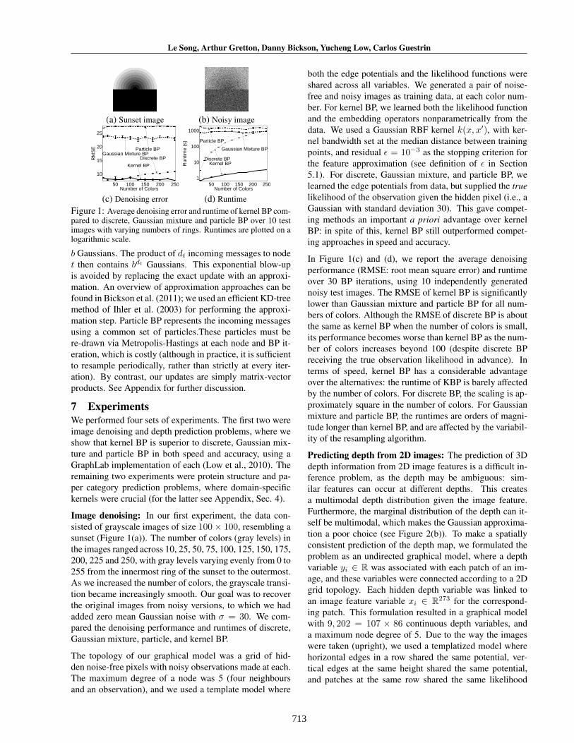
(c) Depth prediction error (d) RuntimeFigure 2: Average depth prediction error and runtime of kernelBP compared to discrete, Gaussian mixture and particle BP over274 images. Runtimes are on a logarithmic scale.

Kernel BP Particle BP0.1

0.2

0.3

0.4

0.5

0.6

Mea

n C

osin

e S

imila

rity

(a) Angle distribution (b) Prediction accuracyFigure 3: Average angle prediction accuracy of kernel versusparticle BP in the protein folding problem.

function. Both the edge potentials between adjacent depthvariables and the likelihood function between image fea-ture and depth were unknown, and were learned from data.

We used a set of 274 images taken on the Stanford campus,including both indoor and outdoor scenes (Saxena et al.,2009). Images were divided into patches of size 107 by 86,with the corresponding depth map for each patch obtainedusing 3D laser scanners (e.g., Figure 2(a)). Each patch wasrepresented by a 273 dimensional feature vector, whichcontained both local features (such as color and texture)and relative features (features from adjacent patches). Wetook the logarithm of the depth map and performed learningand prediction in this space. The entire dataset containedmore than 2 million data points (107 × 86 × 274). Weapplied a Gaussian RBF kernel on the depth information,with the bandwidth parameter set to the median distancebetween training depths, and an approximation residual ofε = 10−3. We used a linear kernel for the image features.

Our results were obtained by leave-one-out cross valida-tion. For each test image, we ran discrete, Gaussian mix-ture, particle, and kernel BP for 10 BP iterations. The aver-age prediction error (MAE: mean absolute error) and run-time are shown in Figures 2(c) and (d). Kernel BP pro-duces the lowest error (MAE=0.145) by a significant mar-gin, while having a similar runtime to discrete BP. Gaussianmixture and particle BP achieve better MAE than discreteBP, but their runtimes are two order of magnitude slower.We note that the error of kernel BP is slightly better than the

results of pointwise MRF reported in Saxena et al. (2009).

Protein structure prediction: Our final experiment inves-tigates the protein folding problem. The folded configu-ration of a protein of length n is roughly determined by asequence of angle pairs {(θi, ωi)}ni=1, each specific to anamino acid position. The goal is to predict the sequenceof angle pairs given only the amino acid sequence. Thetwo angles (θi, ωi) have ranges [0, 180] and (−180, 180]respectively, such that they correspond to points on the unitsphere S2. Kernels yield an immediate solution to infer-ence on these data: Wendland (2005, Theorem 17.10) pro-vides a sufficient condition for a function on S2 to be posi-tive definite, satisfied by k(x, x′) := exp(σ 〈x, x′〉), where〈x, x′〉 is the standard inner product between Euclidean co-ordinates. Given the data are continuous, multimodal, andon a non-Euclidean domain (Figure 3(a)), it is not obvioushow Gaussian mixture or discrete BP might be applied. Wetherefore focus on comparing kernel and particle BP.

We obtained a collection of 1, 400 proteins with lengthlarger than 100 from PDB. We first ran PSI-BLAST to gen-erate the sequence profile (a 20 dimensional feature foreach amino acid position), and then used this profile asfeatures for predicting the folding structure (Jones, 1999).The graphical model was a chain of connected angle pairs,where each angle pair was associated with a 20 dimen-sional feature. We used a linear kernel on the sequence fea-tures. For the kernel between angles, the bandwidth param-eter was set at the median inner product between trainingpoints, and we used the approximation residual ε = 10−3.For particle BP, we learned the nonparametric potentialsusing exp(σ 〈x, x′〉) as the basis functions.

In Figure 3(b), we report the average prediction accuracy(Mean Cosine Similarity between the true coordinate xand the predicted x′, i.e., 〈x, x′〉) over a 10-fold cross-validation process. In this case, kernel BP achieves a sig-nificantly better result than particle BP while running muchfaster (runtimes not shown due to space constraints).

8 Conclusions and Further WorkWe have introduced kernel belief propagation, where themessages are functions in an RKHS. Kernel BP performslearning and inference on challenging graphical modelswith structured and continuous random variables, and ismore accurate and much faster than earlier nonparametricBP algorithms. A possible extension to this work wouldbe to kernelize tree-reweighted belief propagation (Wain-wright et al., 2003). The convergence of kernel BP is a fur-ther challenging topic for future work (Ihler et al., 2005).

Acknowledgements: We thank Alex Ihler for the Gaussianmixture BP codes and helpful discussions. LS is supportedby a Stephenie and Ray Lane Fellowship. This research wasalso supported by ARO MURI W911NF0710287, ARO MURIW911NF0810242, NSF Mundo IIS-0803333, NSF Nets-NBDCNS-0721591 and ONR MURI N000140710747.

715


References

Aronszajn, N. (1950). Theory of reproducing kernels. Trans.Amer. Math. Soc., 68, 337–404.

Bach, F. R., & Jordan, M. I. (2002). Kernel independent compo-nent analysis. J. Mach. Learn. Res., 3, 1–48.

Bickson, D., Baron, D., Ihler, A., Avissar, H., & Dolev, D.(2011). Fault identification via non-parametric belief propa-gation. IEEE Transactions on Signal Processing. ISSN 1053-587X.

Fukumizu, K., Bach, F. R., & Jordan, M. I. (2004). Dimension-ality reduction for supervised learning with reproducing kernelHilbert spaces. J. Mach. Learn. Res., 5, 73–99.

Fukumizu, K., Sriperumbudur, B., Gretton, A., & Schoelkopf, B.(2009). Characteristic kernels on groups and semigroups. InAdvances in Neural Information Processing Systems 21, 473–480. Red Hook, NY: Curran Associates Inc.

Ihler, A., & McAllester, D. (2009). Particle belief propagation. InAISTATS.

Ihler, A. T., Fisher III, J. W., & Willsky, A. S. (2005). Loopybelief propagation: Convergence and effects of message errors.J. Mach. Learn. Res., 6, 905–936.

Ihler, E. T., Sudderth, E. B., Freeman, W. T., & Willsky, A. S.(2003). Efficient multiscale sampling from products of gaus-sian mixtures. In In NIPS 17.

Jones, D. T. (1999). Protein secondary structure prediction basedon position-specific scoring matrices. J. Mol. Biol., 292, 195–202.

Koller, D., & Friedman, N. (2009). Probabilistic Graphical Mod-els: Principles and Techniques. MIT Press.

Low, Y., Gonzalez, J., Kyrola, A., Bickson, D., Guestrin, C., &Hellerstein, J. M. (2010). GraphLab: A new parallel frame-work for machine learning. In Conference on Uncertainty inArtificial Intelligence.

McEliece, R., MacKay, D., & Cheng, J. (1998). Turbo decodingas an instance of Pearl’s belief propagation algorithm. J-SAC.

Murphy, K. P., Weiss, Y., & Jordan, M. I. (1999). Loopy beliefpropagation for approximate inference: An empirical study. InUAI, 467–475.

Pearl, J. (1988). Probabilistic Reasoning in Intelligent Systems:Networks of Plausible Inference. Morgan Kaufman.

Saxena, A., Sun, M., & Ng, A. Y. (2009). Make3d: Learning 3dscene structure from a single still image. IEEE Trans. PatternAnal. Mach. Intell., 31(5), 824–840. ISSN 0162-8828. doi:http://dx.doi.org/10.1109/TPAMI.2008.132.

Scholkopf, B., & Smola, A. (2002). Learning with Kernels. Cam-bridge, MA: MIT Press.

Scholkopf, B., Tsuda, K., & Vert, J.-P. (2004). Kernel Methods inComputational Biology. Cambridge, MA: MIT Press.

Shawe-Taylor, J., & Cristianini, N. (2004). Kernel Methodsfor Pattern Analysis. Cambridge, UK: Cambridge UniversityPress.

Song, L., Gretton, A., & Guestrin, C. (2010). Nonparametric treegraphical models. In 13th Workshop on Artificial Intelligenceand Statistics, vol. 9 of JMLR workshop and conference pro-ceedings, 765–772.

Song, L., Huang, J., Smola, A., & Fukumizu, K. (2009). Hilbertspace embeddings of conditional distributions. In Proc. Intl.Conf. Machine Learning.

Steinwart, I. (2001). On the influence of the kernel on the con-sistency of support vector machines. J. Mach. Learn. Res., 2,67–93.

Sudderth, E., Ihler, A., Freeman, W., & Willsky, A. (2003). Non-parametric belief propagation. In CVPR.

Sugiyama, M., Takeuchi, I., Suzuki, T., Kanamori, T., Hachiya,H., & Okanohara, D. (2010). Conditional density estimationvia least-squares density ratio estimation. 781–788.

Wainwright, M., Jaakkola, T., & Willsky, A. (2003). Tree-reweighted belief propagation and approximate ML estimationby pseudo-moment matching. In 9th Workshop on ArtificialIntelligence and Statistics.

Wainwright, M. J., & Jordan, M. I. (2008). Graphical models,exponential families, and variational inference. Foundationsand Trends in Machine Learning, 1(1 – 2), 1 – 305.

Weiss, Y., & Freeman, W. T. (2001). Correctness of belief prop-agation in Gaussian graphical models of arbitrary topology.Neural Computation, 13, 2173–2200.

Wendland, H. (2005). Scattered Data Approximation. Cambridge,UK: Cambridge University Press.

Yanover, C., & Weiss, Y. (2002). Approximate inference andprotein-folding. In NIPS, 1457–1464. MIT Press.

Yedidia, J. S., Freeman, W. T., & Weiss, Y. (2001). Generalizedbelief propagation. In T. K. Leen, T. G. Dietterich, & V. Tresp,eds., Advances in Neural Information Processing Systems 13,689–695. MIT Press.

Documents

Kernel Belief Propagation