Nonparametric BeliefPropagation and FacialAppearance Estimation

Erik B. Sudderth, Alexander T. Ihler, William T. Freeman and Alan S. Willsky

AI Memo 2002-020 December 2002

© 2 0 0 2 m a s s a c h u s e t t s i n s t i t u t e o f t e c h n o l o g y, c a m b r i d g e , m a 0 2 1 3 9 u s a — w w w. a i . m i t . e d u

m a s s a c h u s e t t s i n s t i t u t e o f t e c h n o l o g y — a r t i f i c i a l i n t e l l i g e n c e l a b o r a t o r y

@ MIT

Abstract

In many applications of graphical models arising in computer vision, the hidden variables of interestare most naturally specified by continuous, non-Gaussian distributions. There exist inference algorithmsfor discrete approximations to these continuous distributions, but for the high-dimensional variablestypically of interest, discrete inference becomes infeasible. Stochastic methods such as particle filtersprovide an appealing alternative. However, existing techniques fail to exploit the rich structure of thegraphical models describing many vision problems.

Drawing on ideas from regularized particle filters and belief propagation (BP), this paper developsa nonparametric belief propagation (NBP) algorithm applicable to general graphs. Each NBP itera-tion uses an efficient sampling procedure to update kernel-based approximations to the true, continuouslikelihoods. The algorithm can accomodate an extremely broad class of potential functions, includingnonparametric representations. Thus, NBP extends particle filtering methods to the more general visionproblems that graphical models can describe. We apply the NBP algorithm to infer component interre-lationships in a parts-based face model, allowing location and reconstruction of occluded features.

This report describes research done within the Laboratory for Information and Decision Systems and the Artificial Intelli-gence Laboratory at the Massachusetts Institute of Technology. This research was supported in part by ONR under GrantN00014-00-1-0089, by AFOSR under Grant F49620-00-1-0362, and by an ODDR&E MURI funded through ARO GrantDAAD19-00-1-0466. E. S. was partially funded by an NDSEG fellowship.

1

1. IntroductionGraphical models provide a powerful, general frameworkfor developing statistical models of computer vision prob-lems [7, 9, 10]. However, graphical formulations are onlyuseful when combined with efficient algorithms for infer-ence and learning. Computer vision problems are par-ticularly challenging because they often involve high–dimensional, continuous variables and complex, multi-modal distributions. For example, the articulated modelsused in many tracking applications have dozens of degreesof freedom to be estimated at each time step [18]. Realis-tic graphical models for these problems must represent out-liers, bimodalities, and other non–Gaussian statistical fea-tures. The corresponding optimal inference procedures forthese models typically involve integral equations for whichno closed form solution exists. Thus, it is necessary to de-velop families of approximate representations, and corre-sponding methods for updating those approximations.

The simplest method for approximating intractablecontinuous–valued graphical models is discretization. Al-though exact inference in general discrete graphs is NPhard [2], approximate inference algorithms such as loopybelief propagation (BP) [17, 22, 24, 25] have been shown toproduce excellent empirical results in many cases. Certainvision problems, including stereo vision [21] and phase un-wrapping [8], are well suited to discrete formulations. Forproblems involving high–dimensional variables, however,exhaustive discretization of the state space is intractable.In some cases, domain–specific heuristics may be used todynamically exclude those configurations which appear un-likely based upon the local evidence [3, 7]. In more chal-lenging vision applications, however, the local evidence atsome nodes may be inaccurate or misleading, and these ap-proaches will heavily distort the computed estimates.

For temporal inference problems, particle filters [6, 10]have proven to be an effective, and influential, alternative todiscretization. They provide the basis for several of the mosteffective visual tracking algorithms [15, 18]. Particle fil-ters approximate conditional densities nonparametrically asa collection of representative elements. Although it is possi-ble to update these approximations deterministically usinglocal linearizations [1], most implementations use MonteCarlo methods to stochastically update a set of weightedpoint samples. The stability and robustness of particle fil-ters can often be improved by regularization methods [6,Chapter 12] in which smoothing kernels [16, 19] explicitlyrepresent the uncertainty associated with each point sample.

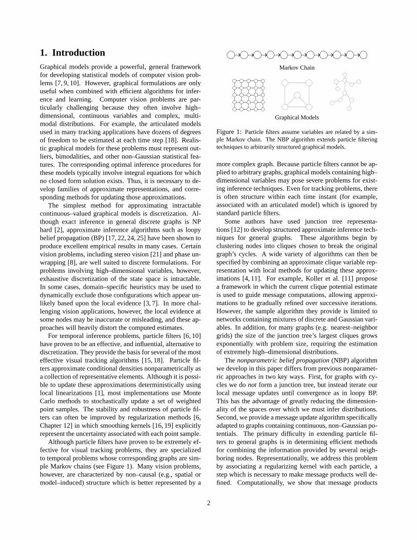
Although particle filters have proven to be extremely ef-fective for visual tracking problems, they are specializedto temporal problems whose corresponding graphs are sim-ple Markov chains (see Figure 1). Many vision problems,however, are characterized by non–causal (e.g., spatial ormodel–induced) structure which is better represented by a

Markov Chain

Graphical Models

Figure 1: Particle filters assume variables are related by a sim-ple Markov chain. The NBP algorithm extends particle filteringtechniques to arbitrarily structured graphical models.

more complex graph. Because particle filters cannot be ap-plied to arbitrary graphs, graphical models containing high–dimensional variables may pose severe problems for exist-ing inference techniques. Even for tracking problems, thereis often structure within each time instant (for example,associated with an articulated model) which is ignored bystandard particle filters.

Some authors have used junction tree representa-tions [12] to develop structured approximate inference tech-niques for general graphs. These algorithms begin byclustering nodes into cliques chosen to break the originalgraph’s cycles. A wide variety of algorithms can then bespecified by combining an approximate clique variable rep-resentation with local methods for updating these approx-imations [4, 11]. For example, Koller et al. [11] proposea framework in which the current clique potential estimateis used to guide message computations, allowing approxi-mations to be gradually refined over successive iterations.However, the sample algorithm they provide is limited tonetworks containing mixtures of discrete and Gaussian vari-ables. In addition, for many graphs (e.g. nearest–neighborgrids) the size of the junction tree’s largest cliques growsexponentially with problem size, requiring the estimationof extremely high–dimensional distributions.

The nonparametric belief propagation (NBP) algorithmwe develop in this paper differs from previous nonparamet-ric approaches in two key ways. First, for graphs with cy-cles we do not form a junction tree, but instead iterate ourlocal message updates until convergence as in loopy BP.This has the advantage of greatly reducing the dimension-ality of the spaces over which we must infer distributions.Second, we provide a message update algorithm specificallyadapted to graphs containing continuous, non–Gaussian po-tentials. The primary difficulty in extending particle fil-ters to general graphs is in determining efficient methodsfor combining the information provided by several neigh-boring nodes. Representationally, we address this problemby associating a regularizing kernel with each particle, astep which is necessary to make message products well de-fined. Computationally, we show that message products

2

may be computed using an efficient local Gibbs samplingprocedure. The NBP algorithm may be applied to arbitrar-ily structured graphs containing a broad range of potentialfunctions, effectively extending particle filtering methods toa much broader range of vision problems.

Following our presentation of the NBP algorithm, wevalidate its performance on a small Gaussian network. Wethen show how NBP may be combined with parts–based lo-cal appearance models [5, 14, 23] to locate and reconstructoccluded facial features.

2. Undirected Graphical ModelsAn undirected graph G is defined by a set of nodes V , and acorresponding set of edges E . The neighborhood of a nodes ∈ V is defined as Γ(s) , {t|(s, t) ∈ E}, the set of allnodes which are directly connected to s. Graphical modelsassociate each node s ∈ V with an unobserved, or hidden,random variable xs, as well as a noisy local observation ys.Let x = {xs}s∈V and y = {ys}s∈V denote the sets of allhidden and observed variables, respectively. To simplifythe presentation, we consider models with pairwise poten-tial functions, for which p (x, y) factorizes as

p (x, y) =1

Z

∏

(s,t)∈E

ψs,t (xs, xt)∏

s∈V

ψs (xs, ys) (1)

However, the nonparametric updates we present may be di-rectly extended to models with higher–order potential func-tions.

In this paper, we focus on the calculation of the condi-tional marginal distributions p (xs | y) for all nodes s ∈ V .These densities provide not only estimates of xs, but alsocorresponding measures of uncertainty.

2.1. Belief PropagationFor graphs which are acyclic or tree–structured, the desiredconditional distributions p (xs | y) can be directly calcu-lated by a local message–passing algorithm known as beliefpropagation (BP) [17, 25]. At iteration n of the BP algo-rithm, each node t ∈ V calculates a message mn

ts (xs) to besent to each neighboring node s ∈ Γ(t):

mnts (xs) = α

∫

xt

ψs,t (xs, xt)ψt (xt, yt)

×∏

u∈Γ(t)\s

mn−1ut (xt) dxt (2)

Here, α denotes an arbitrary proportionality constant. Atany iteration, each node can produce an approximationpn(xs | y) to the marginal distributions p (xs | y) by com-bining the incoming messages with the local observation

potential:

pn(xs | y) = αψs (xs, ys)∏

t∈Γ(s)

mnts (xs) (3)

For tree–structured graphs, the approximate marginals, orbeliefs, pn(xs | y) will converge to the true marginalsp (xs | y) once the messages from each node have propa-gated to every other node in the graph.

Because each iteration of the BP algorithm involves onlylocal message updates, it can be applied even to graphswith cycles. For such graphs, the statistical dependenciesbetween BP messages are not properly accounted for, andthe sequence of beliefs pn(xs | y) will not converge to thetrue marginal distributions. In many applications, however,the resulting loopy BP algorithm exhibits excellent empir-ical performance [7, 8]. Recently, several theoretical stud-ies have provided insight into the approximations made byloopy BP, partially justifying its application to graphs withcycles [22, 24, 25].

2.2. Nonparametric RepresentationsExact evaluation of the BP update equation (2) involves anintegration which, as discussed in the Introduction, is notanalytically tractable for most continuous hidden variables.An interesting alternative is to represent the resulting mes-sage mts (xs) nonparametrically as a kernel–based densityestimate [16, 19]. Let N (x;µ,Λ) denote the value of aGaussian density of mean µ and covariance Λ at the pointx. We may then approximate mts (xs) by a mixture of MGaussian kernels as

mts (xs) =M∑

i=1

w(i)s N

(

xs;µ(i)s ,Λs

)

(4)

where w(i)s is the weight associated with the ith kernel

mean µ(i)s , and Λs is a bandwidth or smoothing parameter.

Other choices of kernel functions are possible [19], but inthis paper we restrict our attention to mixtures of diagonal–covariance Gaussians.

In the following section, we describe stochastic meth-ods for determining the kernel centers µ

(i)s and associ-

ated weights w(i)s . The resulting nonparametric represen-

tations are only meaningful when the messages mts (xs)are finitely integrable.1 To guarantee this, it is sufficient toassume that all potentials satisfy the following constraints:

∫

xs

ψs,t (xs, xt = x) dxs <∞∫

xs

ψs (xs, ys = y) dxs <∞(5)

1Probabilistically, BP messages are likelihood functions mts (xs) ∝

p (y = y | xs), not densities, and are not necessarily integrable (e.g.,when xs and y are independent).

3

Under these assumptions, a simple induction argument willshow that all messages are normalizable. Heuristically,equation (5) requires all potentials to be “informative,” sothat fixing the value of one variable constrains the likely lo-cations of the other. In most application domains, this canbe trivially achieved by assuming that all hidden variablestake values in a large, but bounded, range.

3. Nonparametric Message UpdatesConceptually, the BP update equation (2) naturally de-composes into two stages. First, the message prod-uct ψt (xt, yt)

∏

umn−1ut (xt) combines information from

neighboring nodes with the local evidence yt, producinga function summarizing all available knowledge about thehidden variable xt. We will refer to this summary asa likelihood function, even though this interpretation isonly strictly correct for an appropriately factorized tree–structured graph. Second, this likelihood function is com-bined with the compatibility potential ψs,t (xs, xt), andthen integrated to produce likelihoods for xs. The non-parametric belief propagation (NBP) algorithm stochasti-cally approximates these two stages, producing consistentnonparametric representations of the messages mts (xs).Approximate marginals p(xs | y) may then be determinedfrom these messages by applying the following section’sstochastic product algorithm to equation (3).

3.1. Message ProductsFor the moment, assume that the local observation poten-tials ψt (xt, yt) are represented by weighted Gaussian mix-tures (such potentials arise naturally from learning–basedapproaches to model identification [7]). The product of dGaussian densities is itself Gaussian, with mean and covari-ance given by

d∏

j=1

N (x;µj ,Λj) ∝ N(

x; µ, Λ)

Λ−1 =

d∑

j=1

Λ−1j Λ−1µ =

d∑

j=1

Λ−1j µj

(6)

Thus, a BP update operation which multiplies d Gaussianmixtures, each containing M components, will produce an-other Gaussian mixture with Md components. The weightw associated with product mixture component N

(

x; µ, Λ)

is given by

w ∝

∏dj=1 wjN (x;µj ,Λj)

N(

x; µ, Λ) (7)

where {wj}dj=1 are the weights associated with the input

Gaussians. Note that equation (7) produces the same value

for any choice of x. Also, in various special cases, such aswhen all input Gaussians have the same variance Λj = Λ,computationally convenient simplifications are possible.

Since integration of Gaussian mixtures is straightfor-ward, in principle the BP message updates could be per-formed exactly by repeated use of equations (6,7). In prac-tice, however, the exponential growth of the number of mix-ture components forces approximations to be made. Givend input mixtures of M Gaussian, the NBP algorithm ap-proximates their Md–component product mixture by draw-ing M independent samples.

Direct sampling from this product, achieved by explic-itly calculating each of the product component weights (7),would require O(Md) operations. The complexity associ-ated with this sampling is combinatorial: each product com-ponent is defined by d labels {lj}d

j=1, where lj identifies akernel in the jth input mixture. Although the joint distribu-tion of the d labels is complex, the conditional distributionof any individual label lj is simple. In particular, assumingfixed values for {lk}k 6=j , equation (7) can be used to samplefrom the conditional distribution of lj in O(M) operations.

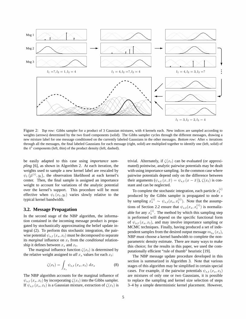
Since the mixture label conditional distributions aretractable, we may use a Gibbs sampler [9] to draw asymp-totically unbiased samples from the product distribution.Details are provided in Algorithm 1, and illustrated in Fig-ure 2. At each iteration, the labels {lk}k 6=j for d − 1 ofthe input mixtures are fixed, and a new value for the jth la-bel is chosen according to equation (7). At the followingiteration, the newly chosen lj is fixed, and another label isupdated. This procedure continues for a fixed number ofiterations κ; more iterations lead to more accurate samples,but require greater computational cost. Following the finaliteration, the mean and covariance of the selected productmixture component is found using equation (6), and a sam-ple point is drawn. To draw M (approximate) samples fromthe product distribution, the Gibbs sampler requires a totalof O(dκM2) operations.

Although formal verification of the Gibbs sampler’s con-vergence is difficult, in our experiments we have observedgood performance using far fewer computations than re-quired by direct sampling. Note that the NBP algorithmuses the Gibbs sampling technique differently from clas-sic simulated annealing procedures [9]. In simulated an-nealing, the Gibbs sampler updates a single Markov chainwhose state dimension is proportional to the graph dimen-sion. In contrast, NBP uses many local Gibbs samplers,each involving only a few nodes. Thus, although NBP mustrun more independent Gibbs samplers, for large graphs thedimensionality of the corresponding Markov chains is dra-matically smaller.

In some applications, the observation potentialsψt (xt, yt) are most naturally specified by analytic func-tions. The previously proposed Gibbs sampler may

4

Msg 1

Msg 2 - -

Msg 3

l1 =?, l2 = 1, l3 = 4 l1 = 4, l2 =?, l3 = 4 l1 = 4, l2 = 3, l3 =?

�

?...

��

���

@@I

l1 = 3, l2 = 2, l3 = 4

Figure 2: Top row: Gibbs sampler for a product of 3 Gaussian mixtures, with 4 kernels each. New indices are sampled according toweights (arrows) determined by the two fixed components (solid). The Gibbs sampler cycles through the different messages, drawing anew mixture label for one message conditioned on the currently labeled Gaussians in the other messages. Bottom row: After κ iterationsthrough all the messages, the final labeled Gaussians for each message (right, solid) are multiplied together to identify one (left, solid) ofthe 43 components (left, thin) of the product density (left, dashed).

be easily adapted to this case using importance sam-pling [6], as shown in Algorithm 2. At each iteration, theweights used to sample a new kernel label are rescaled byψt

(

µ(i), yt

)

, the observation likelihood at each kernel’scenter. Then, the final sample is assigned an importanceweight to account for variations of the analytic potentialover the kernel’s support. This procedure will be mosteffective when ψt (xt, yt) varies slowly relative to thetypical kernel bandwidth.

3.2. Message PropagationIn the second stage of the NBP algorithm, the informa-tion contained in the incoming message product is propa-gated by stochastically approximating the belief update in-tegral (2). To perform this stochastic integration, the pair-wise potential ψs,t (xs, xt) must be decomposed to separateits marginal influence on xt from the conditional relation-ship it defines between xs and xt.

The marginal influence function ζ(xt) is determined bythe relative weight assigned to all xs values for each xt:

ζ(xt) =

∫

xs

ψs,t (xs, xt) dxs (8)

The NBP algorithm accounts for the marginal influence ofψs,t (xs, xt) by incorporating ζ(xt) into the Gibbs sampler.If ψs,t (xs, xt) is a Gaussian mixture, extraction of ζ(xt) is

trivial. Alternately, if ζ(xt) can be evaluated (or approxi-mated) pointwise, analytic pairwise potentials may be dealtwith using importance sampling. In the common case wherepairwise potentials depend only on the difference betweentheir arguments (ψs,t (x, x) = ψs,t (x − x)), ζ(xt) is con-stant and can be neglected.

To complete the stochastic integration, each particle x(i)t

produced by the Gibbs sampler is propagated to node s

by sampling x(i)s ∼ ψs,t(xs, x

(i)t ). Note that the assump-

tions of Section 2.2 ensure that ψs,t(xs, x(i)t ) is normaliz-

able for any x(i)t . The method by which this sampling step

is performed will depend on the specific functional formof ψs,t (xs, xt), and may involve importance sampling orMCMC techniques. Finally, having produced a set of inde-pendent samples from the desired output messagemts (xs),NBP must choose a kernel bandwidth to complete the non-parametric density estimate. There are many ways to makethis choice; for the results in this paper, we used the com-putationally efficient “rule of thumb” heuristic [19].

The NBP message update procedure developed in thissection is summarized in Algorithm 3. Note that variousstages of this algorithm may be simplified in certain specialcases. For example, if the pairwise potentials ψs,t (xs, xt)are mixtures of only one or two Gaussians, it is possibleto replace the sampling and kernel size selection of steps3–4 by a simple deterministic kernel placement. However,

5

Given d mixtures of M Gaussians, where {µ(i)j ,Λ

(i)j , w

(i)j }

Mi=1

denote the parameters of the jth mixture:

1. For each j ∈ [1 : d], choose a starting label lj ∈ [1 : M ] bysampling p (lj = i) ∝ w

(i)j .

2. For each j ∈ [1 : d],

(a) Calculate the mean µ∗ and variance Λ∗ of the product∏

k 6=jN

(

x;µ(lk)k ,Λ

(lk)k

)

using equation (6).

(b) For each i ∈ [1 : M ], calculate the mean µ(i) and vari-

ance Λ(i) of N (x;µ∗,Λ∗) · N(

x;µ(i)j ,Λ

(i)j

)

. Using

any convenient x, compute the weight

w(i) = w(i)j

N(

x;µ(i)j ,Λ

(i)j

)

N (x;µ∗,Λ∗)

N(

x; µ(i), Λ(i))

(c) Sample a new label lj according to p (lj = i) ∝ w(i).

3. Repeat step 2 for κ iterations.

4. Compute the mean µ and variance Λ of the product∏d

j=1N(

x;µ(lj)

j ,Λ(lj)

j

)

. Draw a sample x ∼ N(

x; µ, Λ)

.

Algorithm 1: Gibbs sampler for products of Gaussian mixtures.

Given d mixtures of M Gaussians and an analytic function f(x),follow Algorithm 1 with the following modifications:

2. After part (b), rescale each computed weight by the analyticvalue at the kernel center: w(i) ← f(µ(i))w(i).

5. Assign importance weight w = f(x)/f(µ) to the sampledparticle x.

Algorithm 2: Gibbs sampler for the product of several Gaussianmixtures with an analytic function f(x).

these more sophisticated updates are necessary for graphicalmodels with more expressive priors, such as those used inSection 5.

4. Gaussian Graphical ModelsGaussian graphical models provide one of the few continu-ous distributions for which the BP algorithm may be imple-mented exactly [24]. For this reason, Gaussian models maybe used to test the accuracy of the nonparametric approxi-mations made by NBP. Note that we cannot hope for NBP tooutperform algorithms (like Gaussian BP) designed to takeadvantage of the linear structure underlying Gaussian prob-lems. Instead, our goal is to verify NBP’s performance in asituation where exact comparisons are possible.

We have tested the NBP algorithm on Gaussian modelswith a range of graphical structures, including chains, trees,and grids. Similar results were observed in all cases, sohere we only present data for a single typical 5× 5 nearest–

Given input messages mut (xt) = {µ(i)ut ,Λ

(i)ut , w

(i)ut }

Mi=1 for each

u ∈ Γ(t) \ s, construct an output message mts (xs) as follows:

1. Determine the marginal influence ζ(xt) using equation (8):

(a) If ψs,t (xs, xt) is a Gaussian mixture, ζ(xt) is themarginal over xt.

(b) For analytic ψs,t (xs, xt), determine ζ(xt) by sym-bolic or numeric integration.

2. Draw M independent samples {x(i)t }

Mi=1 from the product

ζ(xt)ψt (xt, yt)∏

umut (xt) using the Gibbs sampler of

Algorithms 1-2.

3. For each {x(i)t }

Mi=1, sample x(i)

s ∼ ψs,t(xs, xt = x(i)t ):

(a) If ψs,t (xs, xt) is a Gaussian mixture, x(i)s is sampled

from the conditional of xs given x(i)t .

(b) For analytic ψs,t (xs, xt), importance sampling orMCMC methods may be used as appropriate.

4. Construct mts (xs) = {µ(i)ts ,Λ

(i)ts , w

(i)ts }

Mi=1:

(a) Set µ(i)ts = x

(i)s , and w

(i)ts equal to the importance

weights (if any) generated in step 3.

(b) Choose {Λ(i)ts }

Mi=1 using any appropriate kernel size

selection method (see [19]).

Algorithm 3: NBP algorithm for updating the nonparametricmessage mts (xs) sent from node t to node s as in equation (2).

neighbor grid (as in Figure 1), with randomly selected inho-mogeneous potential functions. To create the test model, wedrew independent samples from the single correlated Gaus-sian defining each of the graph’s clique potentials, and thenformed a nonparametric density estimate based on thesesamples. Although the NBP algorithm could have directlyused the original correlated potentials, sample–based mod-els are a closer match for the information available in manyvision applications (see Section 5).

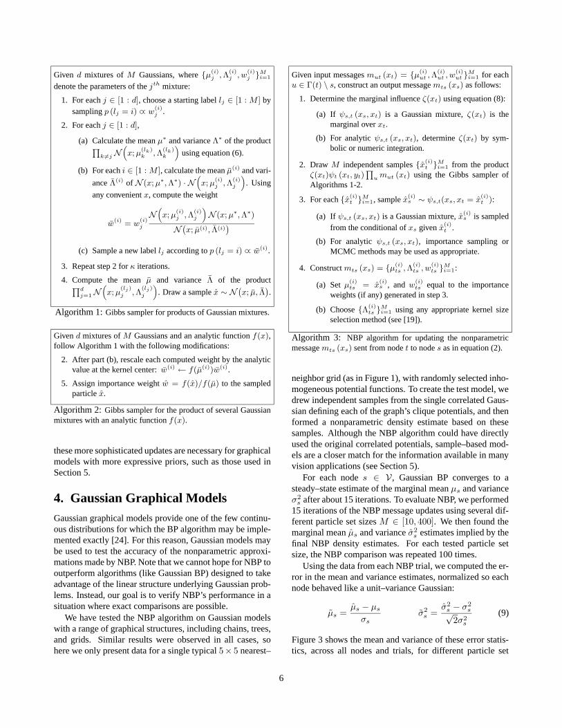
For each node s ∈ V , Gaussian BP converges to asteady–state estimate of the marginal mean µs and varianceσ2

s after about 15 iterations. To evaluate NBP, we performed15 iterations of the NBP message updates using several dif-ferent particle set sizes M ∈ [10, 400]. We then found themarginal mean µs and variance σ2

s estimates implied by thefinal NBP density estimates. For each tested particle setsize, the NBP comparison was repeated 100 times.

Using the data from each NBP trial, we computed the er-ror in the mean and variance estimates, normalized so eachnode behaved like a unit–variance Gaussian:

µs =µs − µs

σsσ2

s =σ2

s − σ2s√

2σ2s

(9)

Figure 3 shows the mean and variance of these error statis-tics, across all nodes and trials, for different particle set

6

0 50 100 150 200 250 300 350 400−1

−0.8

−0.6

−0.4

−0.2

0

0.2

0.4

0.6

0.8

1

Number of Particles (M)0 50 100 150 200 250 300 350 400

0

0.5

1

1.5

2

2.5

Number of Particles (M)

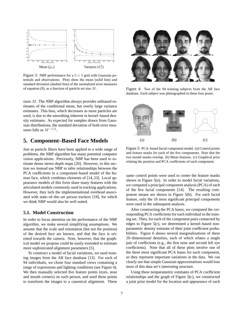
Mean (µs) Variance (σ2s )

Figure 3: NBP performance for a 5 × 5 grid with Gaussian po-tentials and observations. Plots show the mean (solid line) andstandard deviation (dashed line) of the normalized error measuresof equation (9), as a function of particle set size M .

sizes M . The NBP algorithm always provides unbiased es-timates of the conditional mean, but overly large varianceestimates. This bias, which decreases as more particles areused, is due to the smoothing inherent in kernel–based den-sity estimates. As expected for samples drawn from Gaus-sian distributions, the standard deviation of both error mea-sures falls as M−1/2.

5. Component–Based Face ModelsJust as particle filters have been applied to a wide range ofproblems, the NBP algorithm has many potential computervision applications. Previously, NBP has been used to es-timate dense stereo depth maps [20]. However, in this sec-tion we instead use NBP to infer relationships between thePCA coefficients in a component–based model of the hu-man face, which combines elements of [14, 23]. Local ap-pearance models of this form share many features with thearticulated models commonly used in tracking applications.However, they lack the implementational overhead associ-ated with state–of–the–art person trackers [18], for whichwe think NBP would also be well suited.

5.1. Model ConstructionIn order to focus attention on the performance of the NBPalgorithm, we make several simplifying assumptions. Weassume that the scale and orientation (but not the position)of the desired face are known, and that the face is ori-ented towards the camera. Note, however, that the graph-ical model we propose could be easily extended to estimatemore sophisticated alignment parameters [5].

To construct a model of facial variations, we used train-ing images from the AR face database [13]. For each of94 individuals, we chose four standard views containing arange of expressions and lighting conditions (see Figure 4).We then manually selected five feature points (eyes, noseand mouth corners) on each person, and used these pointsto transform the images to a canonical alignment. These

Figure 4: Two of the 94 training subjects from the AR facedatabase. Each subject was photographed in these four poses.

(a) (b) (c)

Figure 5: PCA–based facial component model. (a) Control pointsand feature masks for each of the five components. Note that thetwo mouth masks overlap. (b) Mean features. (c) Graphical priorrelating the position and PCA coefficients of each component.

same control points were used to center the feature masksshown in Figure 5(a). In order to model facial variations,we computed a principal component analysis (PCA) of eachof the five facial components [14]. The resulting com-ponent means are shown in Figure 5(b). For each facialfeature, only the 10 most significant principal componentswere used in the subsequent analysis.

After constructing the PCA bases, we computed the cor-responding PCA coefficients for each individual in the train-ing set. Then, for each of the component pairs connected byedges in Figure 5(c), we determined a kernel–based non-parametric density estimate of their joint coefficient proba-bilities. Figure 6 shows several marginalizations of these20–dimensional densities, each of which relates a singlepair of coefficients (e.g., the first nose and second left eyecoefficients). Note that all of these plots involve one ofthe three most significant PCA bases for each component,so they represent important variations in the data. We canclearly see that simple Gaussian approximations would losemost of this data set’s interesting structure.

Using these nonparametric estimates of PCA coefficientrelationships and the graph of Figure 5(c), we constructeda joint prior model for the location and appearance of each

7

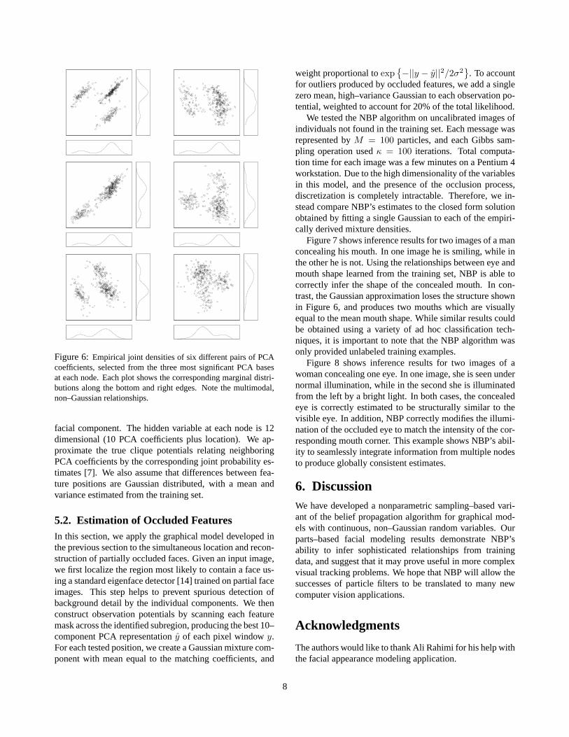
Figure 6: Empirical joint densities of six different pairs of PCAcoefficients, selected from the three most significant PCA basesat each node. Each plot shows the corresponding marginal distri-butions along the bottom and right edges. Note the multimodal,non–Gaussian relationships.

facial component. The hidden variable at each node is 12dimensional (10 PCA coefficients plus location). We ap-proximate the true clique potentials relating neighboringPCA coefficients by the corresponding joint probability es-timates [7]. We also assume that differences between fea-ture positions are Gaussian distributed, with a mean andvariance estimated from the training set.

5.2. Estimation of Occluded FeaturesIn this section, we apply the graphical model developed inthe previous section to the simultaneous location and recon-struction of partially occluded faces. Given an input image,we first localize the region most likely to contain a face us-ing a standard eigenface detector [14] trained on partial faceimages. This step helps to prevent spurious detection ofbackground detail by the individual components. We thenconstruct observation potentials by scanning each featuremask across the identified subregion, producing the best 10–component PCA representation y of each pixel window y.For each tested position, we create a Gaussian mixture com-ponent with mean equal to the matching coefficients, and

weight proportional to exp{

−||y − y||2/2σ2}

. To accountfor outliers produced by occluded features, we add a singlezero mean, high–variance Gaussian to each observation po-tential, weighted to account for 20% of the total likelihood.

We tested the NBP algorithm on uncalibrated images ofindividuals not found in the training set. Each message wasrepresented by M = 100 particles, and each Gibbs sam-pling operation used κ = 100 iterations. Total computa-tion time for each image was a few minutes on a Pentium 4workstation. Due to the high dimensionality of the variablesin this model, and the presence of the occlusion process,discretization is completely intractable. Therefore, we in-stead compare NBP’s estimates to the closed form solutionobtained by fitting a single Gaussian to each of the empiri-cally derived mixture densities.

Figure 7 shows inference results for two images of a manconcealing his mouth. In one image he is smiling, while inthe other he is not. Using the relationships between eye andmouth shape learned from the training set, NBP is able tocorrectly infer the shape of the concealed mouth. In con-trast, the Gaussian approximation loses the structure shownin Figure 6, and produces two mouths which are visuallyequal to the mean mouth shape. While similar results couldbe obtained using a variety of ad hoc classification tech-niques, it is important to note that the NBP algorithm wasonly provided unlabeled training examples.

Figure 8 shows inference results for two images of awoman concealing one eye. In one image, she is seen undernormal illumination, while in the second she is illuminatedfrom the left by a bright light. In both cases, the concealedeye is correctly estimated to be structurally similar to thevisible eye. In addition, NBP correctly modifies the illumi-nation of the occluded eye to match the intensity of the cor-responding mouth corner. This example shows NBP’s abil-ity to seamlessly integrate information from multiple nodesto produce globally consistent estimates.

6. DiscussionWe have developed a nonparametric sampling–based vari-ant of the belief propagation algorithm for graphical mod-els with continuous, non–Gaussian random variables. Ourparts–based facial modeling results demonstrate NBP’sability to infer sophisticated relationships from trainingdata, and suggest that it may prove useful in more complexvisual tracking problems. We hope that NBP will allow thesuccesses of particle filters to be translated to many newcomputer vision applications.

Acknowledgments

The authors would like to thank Ali Rahimi for his help withthe facial appearance modeling application.

8

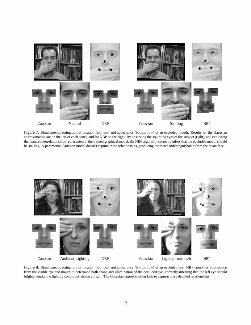
Gaussian Neutral NBP Gaussian Smiling NBP

Figure 7: Simultaneous estimation of location (top row) and appearance (bottom row) of an occluded mouth. Results for the Gaussianapproximation are on the left of each panel, and for NBP on the right. By observing the squinting eyes of the subject (right), and exploitingthe feature interrelationships represented in the trained graphical model, the NBP algorithm correctly infers that the occluded mouth shouldbe smiling. A parametric Gaussian model doesn’t capture these relationships, producing estimates indistinguishable from the mean face.

Gaussian Ambient Lighting NBP Gaussian Lighted from Left NBP

Figure 8: Simultaneous estimation of location (top row) and appearance (bottom row) of an occluded eye. NBP combines informationfrom the visible eye and mouth to determine both shape and illumination of the occluded eye, correctly inferring that the left eye shouldbrighten under the lighting conditions shown at right. The Gaussian approximation fails to capture these detailed relationships.

9

References

[1] D. L. Alspach and H. W. Sorenson. NonlinearBayesian estimation using Gaussian sum approxima-tions. IEEE Trans. AC, 17(4):439–448, August 1972.

[2] G. Cooper. The computational complexity of proba-bilistic inference using Bayesian belief networks. Ar-tificial Intelligence, 42:393–405, 1990.

[3] J. M. Coughlan and S. J. Ferreira. Finding deformableshapes using loopy belief propagation. In ECCV,pages 453–468, 2002.

[4] A. P. Dawid, U. Kjærulff, and S. L. Lauritzen. Hybridpropagation in junction trees. In Adv. Intell. Comp.,pages 87–97, 1995.

[5] F. De la Torre and M. J. Black. Robust parameterizedcomponent analysis: Theory and applications to 2Dfacial modeling. In ECCV, pages 653–669, 2002.

[6] A. Doucet, N. de Freitas, and N. Gordon, editors. Se-quential Monte Carlo Methods in Practice. Springer-Verlag, New York, 2001.

[7] W. T. Freeman, E. C. Pasztor, and O. T. Carmichael.Learning low–level vision. IJCV, 40(1):25–47, 2000.

[8] B. J. Frey, R. Koetter, and N. Petrovic. Very loopybelief propagation for unwrapping phase images. InNIPS 14. MIT Press, 2002.

[9] S. Geman and D. Geman. Stochastic relaxation, Gibbsdistributions, and the Bayesian restoration of images.IEEE Trans. PAMI, 6(6):721–741, November 1984.

[10] M. Isard and A. Blake. Contour tracking by stochasticpropagation of conditional density. In ECCV, pages343–356, 1996.

[11] D. Koller, U. Lerner, and D. Angelov. A general algo-rithm for approximate inference and its application tohybrid Bayes nets. In UAI 15, pages 324–333, 1999.

[12] S. L. Lauritzen. Graphical Models. Oxford UniversityPress, 1996.

[13] A. M. Martınez and R. Benavente. The AR facedatabase. Technical Report 24, CVC, June 1998.

[14] B. Moghaddam and A. Pentland. Probabilistic visuallearning for object representation. IEEE Trans. PAMI,19(7):696–710, July 1997.

[15] O. Nestares and D. J. Fleet. Probabilistic tracking ofmotion boundaries with spatiotemporal predictions. InCVPR, pages 358–365, 2001.

[16] E. Parzen. On estimation of a probability density func-tion and mode. Ann. of Math Stats., 33:1065–1076,1962.

[17] J. Pearl. Probabilistic Reasoning in Intelligent Sys-tems. Morgan Kaufman, San Mateo, 1988.

[18] H. Sidenbladh and M. J. Black. Learning the statis-tics of people in images and video. IJCV, 2002. Inrevision.

[19] B. W. Silverman. Density Estimation for Statistics andData Analysis. Chapman & Hall, London, 1986.

[20] E. B. Sudderth, A. T. Ihler, W. T. Freeman, and A. S.Willsky. Nonparametric belief propagation. Techni-cal Report 2551, MIT Laboratory for Information andDecision Systems, October 2002.

[21] J. Sun, H. Shum, and N. Zheng. Stereo matching usingbelief propagation. In ECCV, pages 510–524, 2002.

[22] M. J. Wainwright, T. Jaakkola, and A. S. Willsky.Tree–based reparameterization for approximate infer-ence on loopy graphs. In NIPS 14. MIT Press, 2002.

[23] M. Weber, M. Welling, and P. Perona. Unsupervisedlearning of models for recognition. In ECCV, 2000.

[24] Y. Weiss and W. T. Freeman. Correctness of beliefpropagation in Gaussian graphical models of arbitrarytopology. Neural Comp., 13:2173–2200, 2001.

[25] J. S. Yedidia, W. T. Freeman, and Y. Weiss. Con-structing free energy approximations and generalizedbelief propagation algorithms. Technical Report 2002-35, Mitsubishi Electric Research Laboratories, August2002.

10