Embed Size (px)
Citation preview
Belief Propagation
by Jakob Metzler
Outline
Motivation Pearl’s BP Algorithm Turbo Codes Generalized Belief Propagation
Free Energies
Probabilistic Inference
From the lecture we know:
Computing the a posteriori belief of a variable in a general Bayesian Network is NP-hard
Solution: approximate inference MCMC sampling
Probabilistic Inference
From the lecture we know:
Computing the a posteriori belief of a variable in a general Bayesian Network is NP-hard
Solution: approximate inference MCMC sampling Belief Propagation
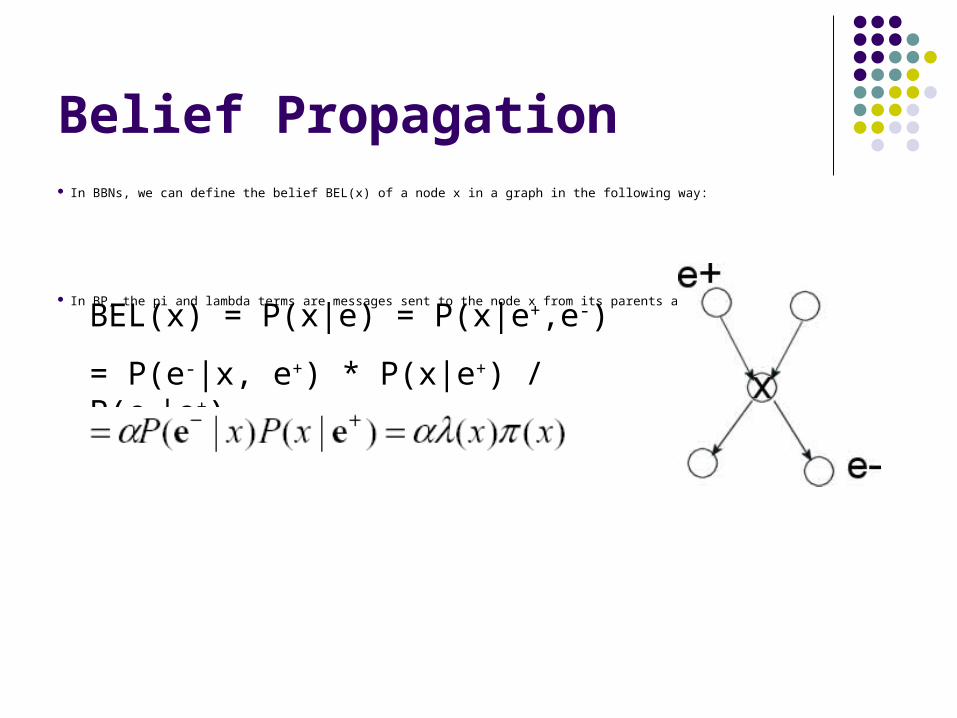
Belief Propagation In BBNs, we can define the belief BEL(x) of a node x in a graph in the following way:
In BP, the pi and lambda terms are messages sent to the node x from its parents and children, respectivelyBEL(x) = P(x|e) = P(x|e+,e-)
= P(e-|x, e+) * P(x|e+) / P(e-|e+)
Pearl’s BP Algorithm
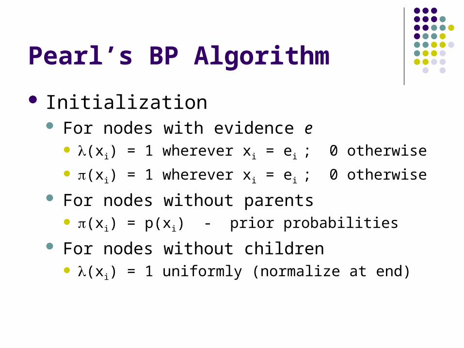
Initialization For nodes with evidence e
(xi) = 1 wherever xi = ei ; 0 otherwise
(xi) = 1 wherever xi = ei ; 0 otherwise
For nodes without parents (xi) = p(xi) - prior probabilities
For nodes without children (xi) = 1 uniformly (normalize at end)
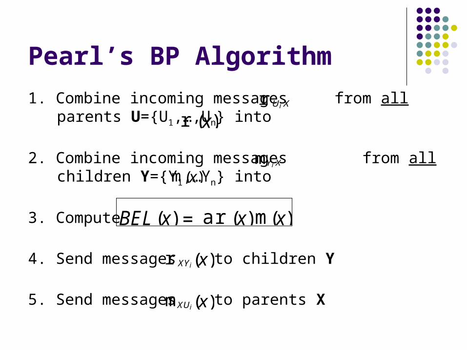
Pearl’s BP Algorithm
1. Combine incoming messages from all parents U={U1,…,Un} into
2. Combine incoming messages from all children Y={Y1,…Yn} into
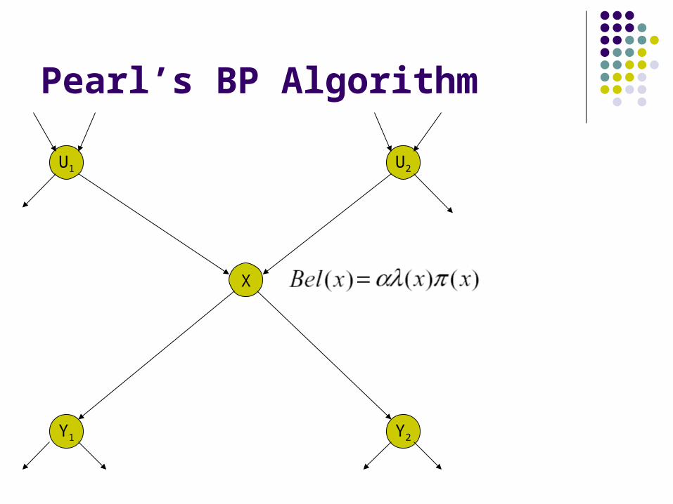
3. Compute
4. Send messages to children Y
5. Send messages to parents X
r Uj X
mYj X
m(x)
r (x)
BEL (x) = ar (x)m(x)
r XYj(x)
mXUj(x)
Pearl’s BP Algorithm
X
U2
Y1 Y2
U1
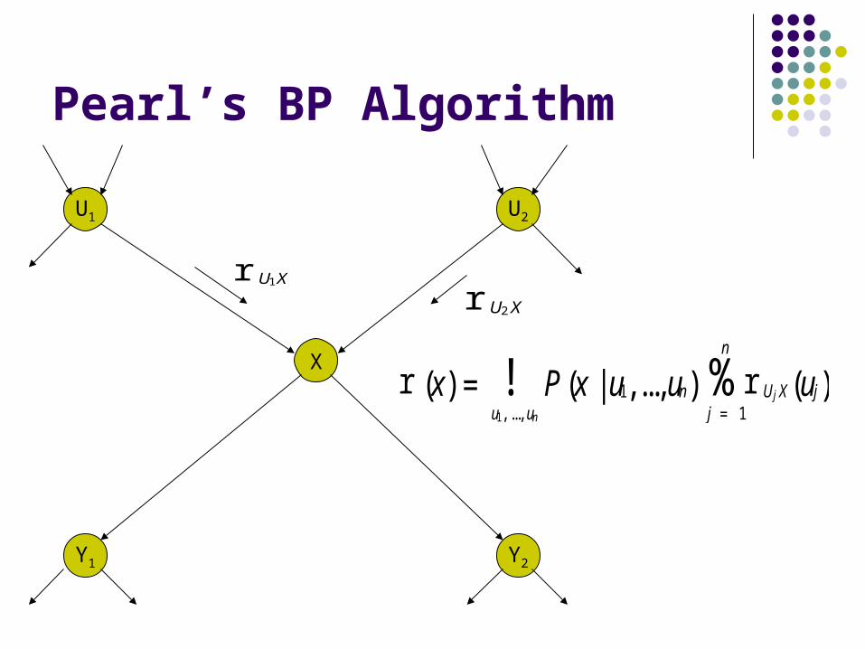
r (x) =u1, ..., un
! P (x |u1,...,un) r Uj X(uj)j = 1
n
%
r U1X
r U2X
Pearl’s BP Algorithm
X
U2
Y1 Y2
U1
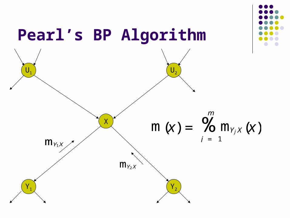
m(x) = mYj X(x)j = 1
m
%mY1X
mY2X
Pearl’s BP Algorithm
X
U2
Y1 Y2
U1
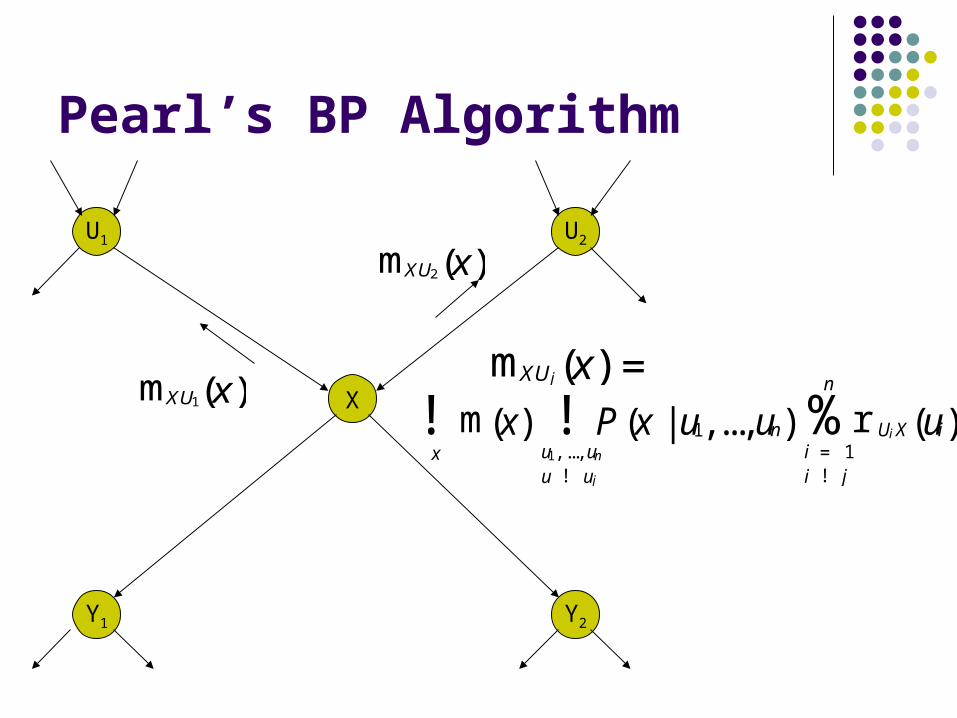
Pearl’s BP Algorithm
X
U2
Y1 Y2
U1
mXU1(x)
mXU2(x)
m(x)x
! P (x |u1,...,un)u1, ..., unu ! uj
! r UiX(ui)i = 1i ! j
n
%mXUj(x) =
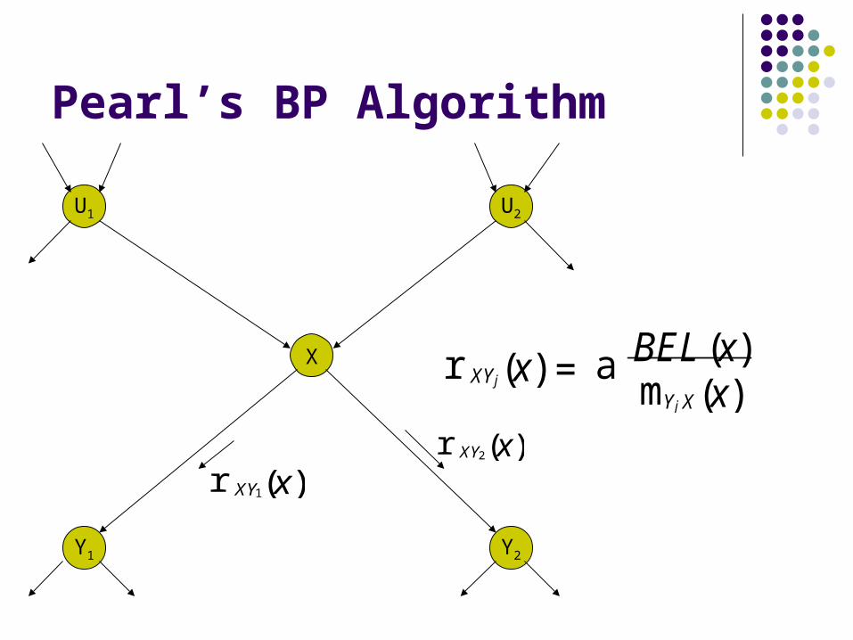
Pearl’s BP Algorithm
X
U2
Y1 Y2
U1
r XY1(x)r XY2(x)
r XYj(x) = amYj X(x)BEL (x)
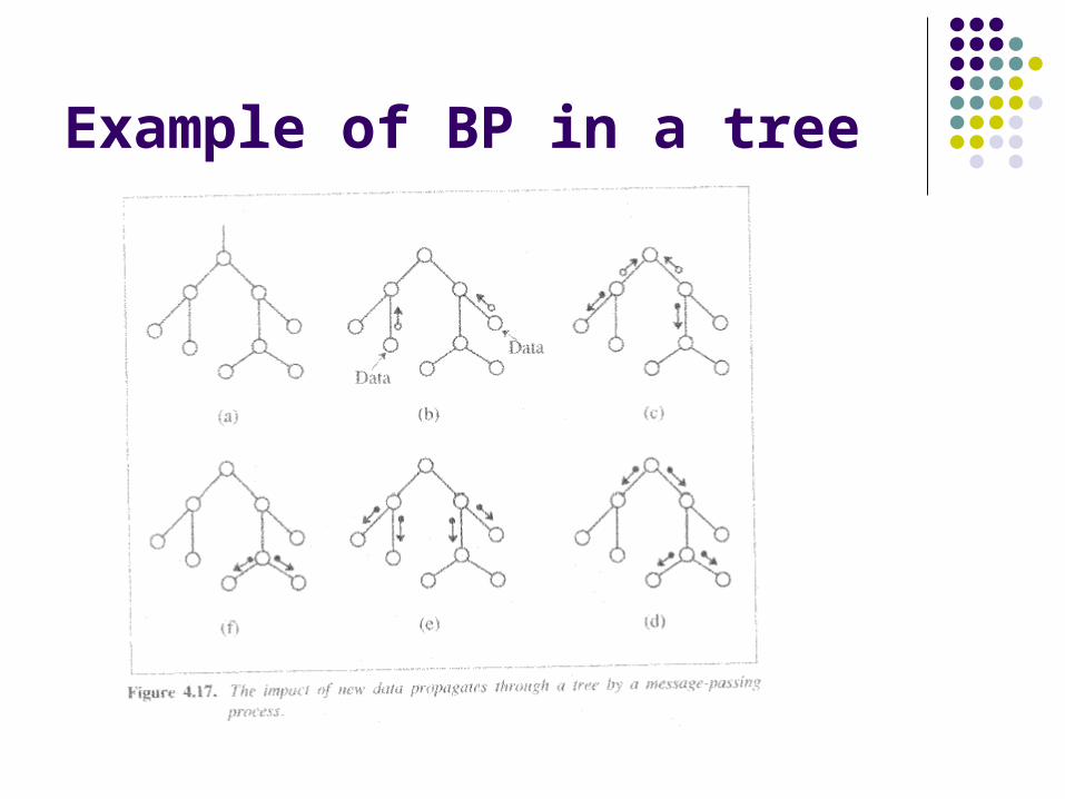
Example of BP in a tree
Properties of BP
Exact for polytrees Each node separates Graph into 2 disjoint
components On a polytree, the BP algorithm converges in time
proportional to diameter of network – at most linear Work done in a node is proportional to the size of CPT
Hence BP is linear in number of network parameters For general BBNs
Exact inference is NP-hard Approximate inference is NP-hard
Properties of BP
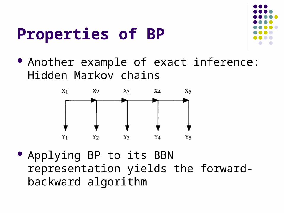
Another example of exact inference: Hidden Markov chains
Applying BP to its BBN representation yields the forward-backward algorithm
Loopy Belief Propagation
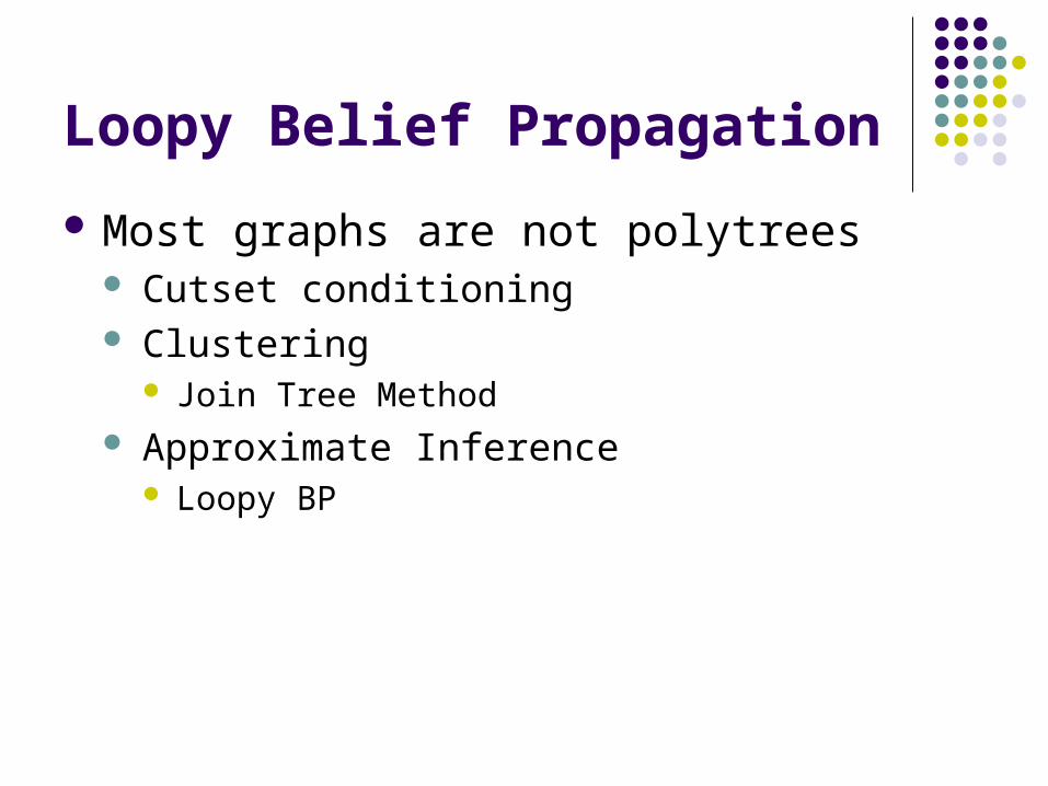
Most graphs are not polytrees Cutset conditioning Clustering
Join Tree Method Approximate Inference
Loopy BP
Loopy Belief Propagation
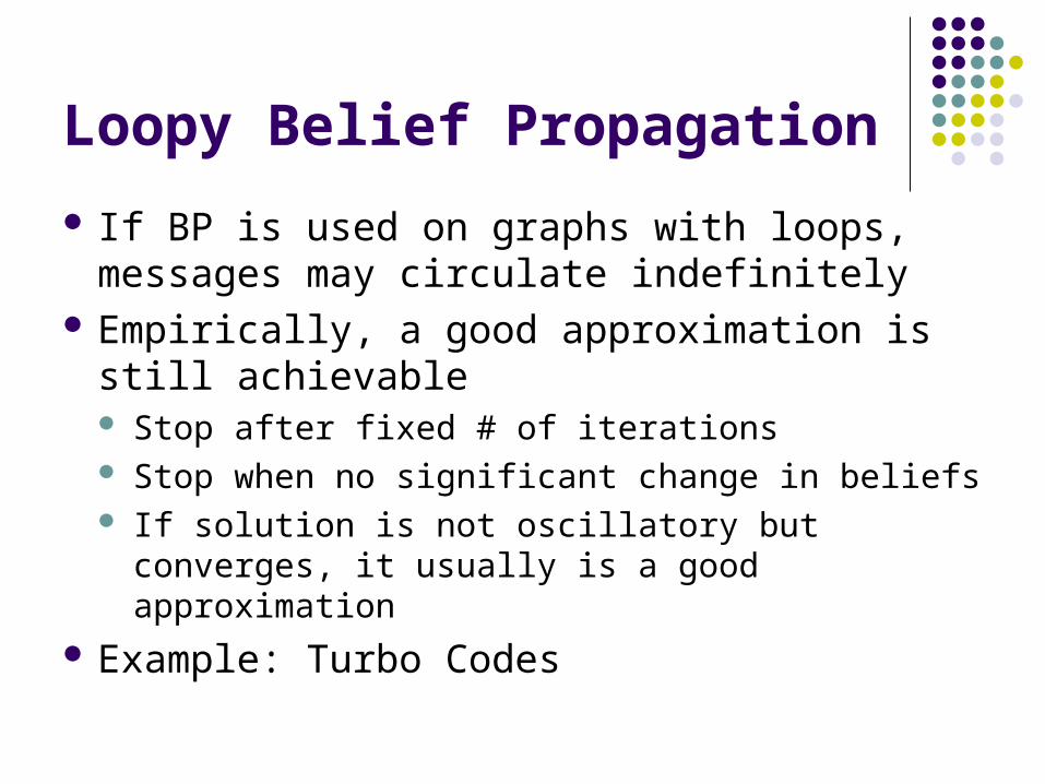
If BP is used on graphs with loops, messages may circulate indefinitely
Empirically, a good approximation is still achievable Stop after fixed # of iterations Stop when no significant change in beliefs If solution is not oscillatory but converges, it
usually is a good approximation Example: Turbo Codes
Outline
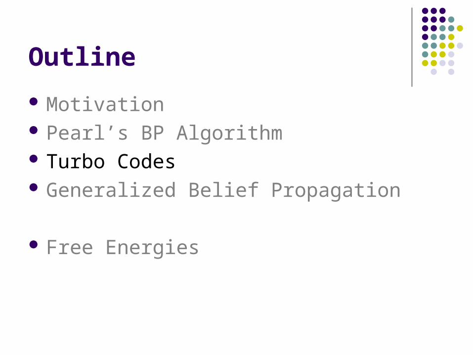
Motivation Pearl’s BP Algorithm Turbo Codes Generalized Belief Propagation
Free Energies
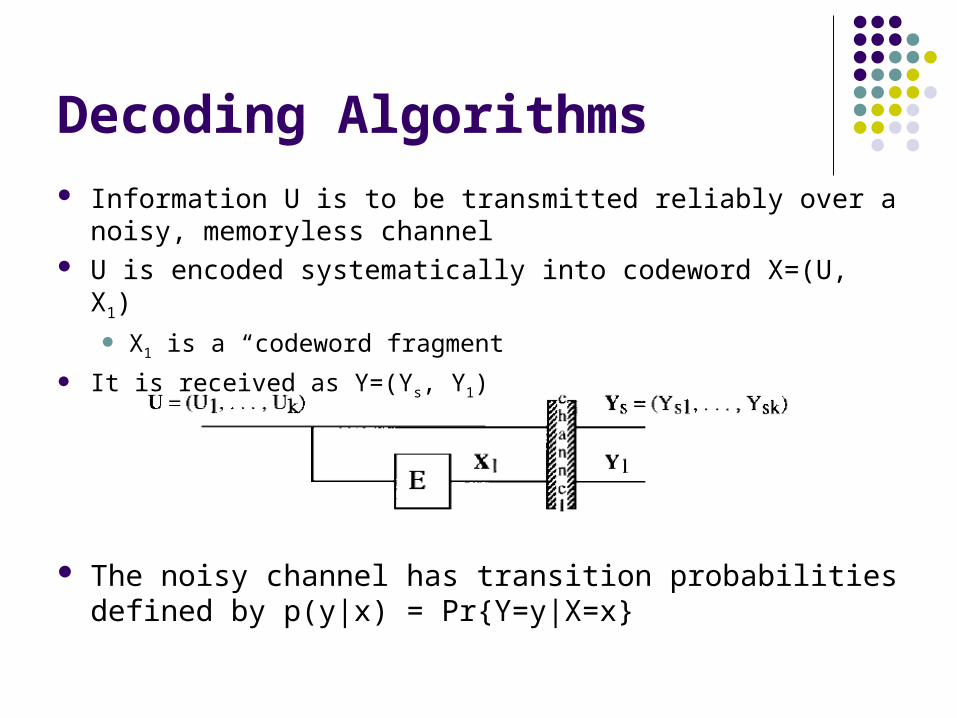
Decoding Algorithms Information U is to be transmitted reliably over a noisy,
memoryless channel U is encoded systematically into codeword X=(U, X1)
X1 is a “codeword fragment
It is received as Y=(Ys, Y1)
The noisy channel has transition probabilities defined by p(y|x) = Pr{Y=y|X=x}
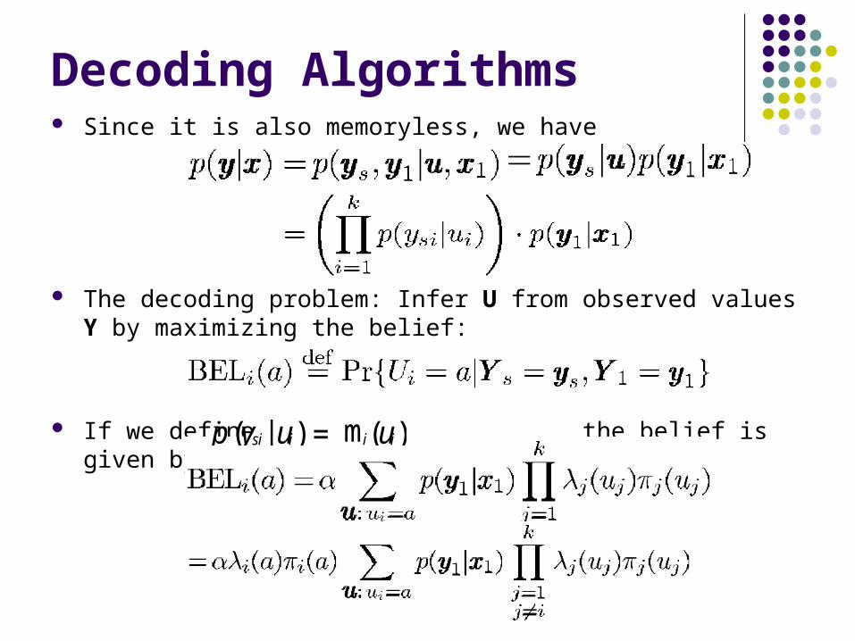
Decoding Algorithms Since it is also memoryless, we have
The decoding problem: Infer U from observed values Y by maximizing the belief:
If we define the belief is given byp(ysi|ui) =mi(ui)
Decoding using BP
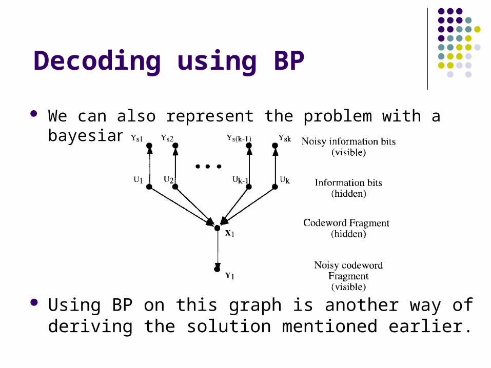
We can also represent the problem with a bayesian network:
Using BP on this graph is another way of deriving the solution mentioned earlier.
Turbo Codes
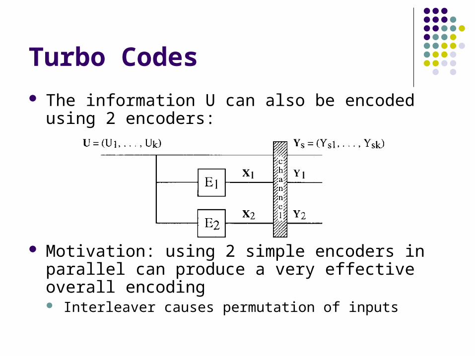
The information U can also be encoded using 2 encoders:
Motivation: using 2 simple encoders in parallel can produce a very effective overall encoding Interleaver causes permutation of inputs
Turbo Codes
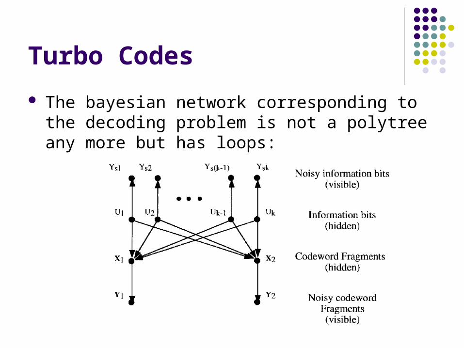
The bayesian network corresponding to the decoding problem is not a polytree any more but has loops:
Turbo Codes
We can still approximate the optimal beliefs by using loopy Belief Propagation Stop after # of iterations
Choosing the order of belief updates among the nodes derives “different” previously known algorithms Sequence U->X1->U->X2->U->X1->U etc. yields the well-
known turbo decoding algorithm Sequence U->X->U->X->U etc. yields a general decoding
algorithm for multiple turbo codes and many more
Turbo Codes Summary
BP can be used as a general decoding algorithm by representing the problem as a BBN and running BP on it.
Many existing, seemingly different decoding algorithms are just instantiations of BP.
Turbo codes are a good example of successful convergence of BP on a loopy graph.
Outline
Motivation Pearl’s BP Algorithm Turbo Codes Generalized Belief Propagation
Free Energies
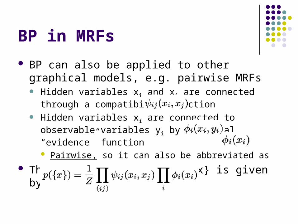
BP in MRFs
BP can also be applied to other graphical models, e.g. pairwise MRFs Hidden variables xi and xj are connected through a
compatibility function Hidden variables xi are connected to observable variables
yi by the local “evidence” function Pairwise, so it can also be abbreviated as
The joint probability of {x} is given by
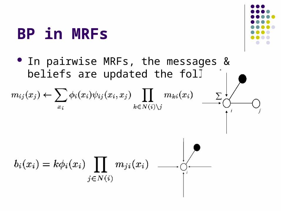
BP in MRFs
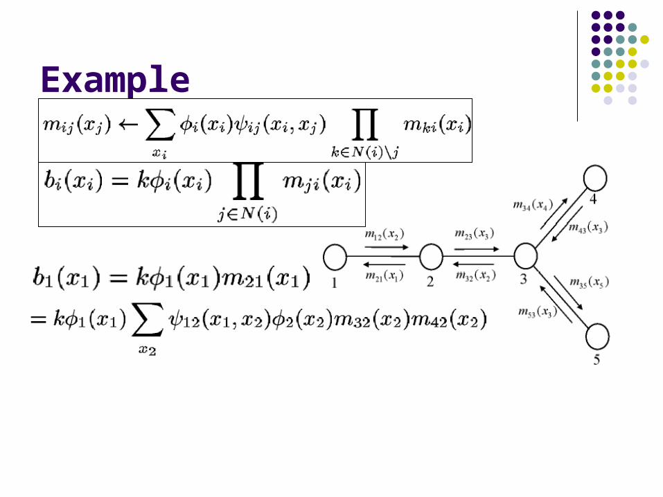
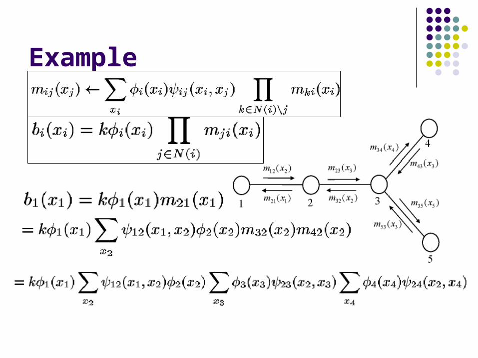
In pairwise MRFs, the messages & beliefs are updated the following way:
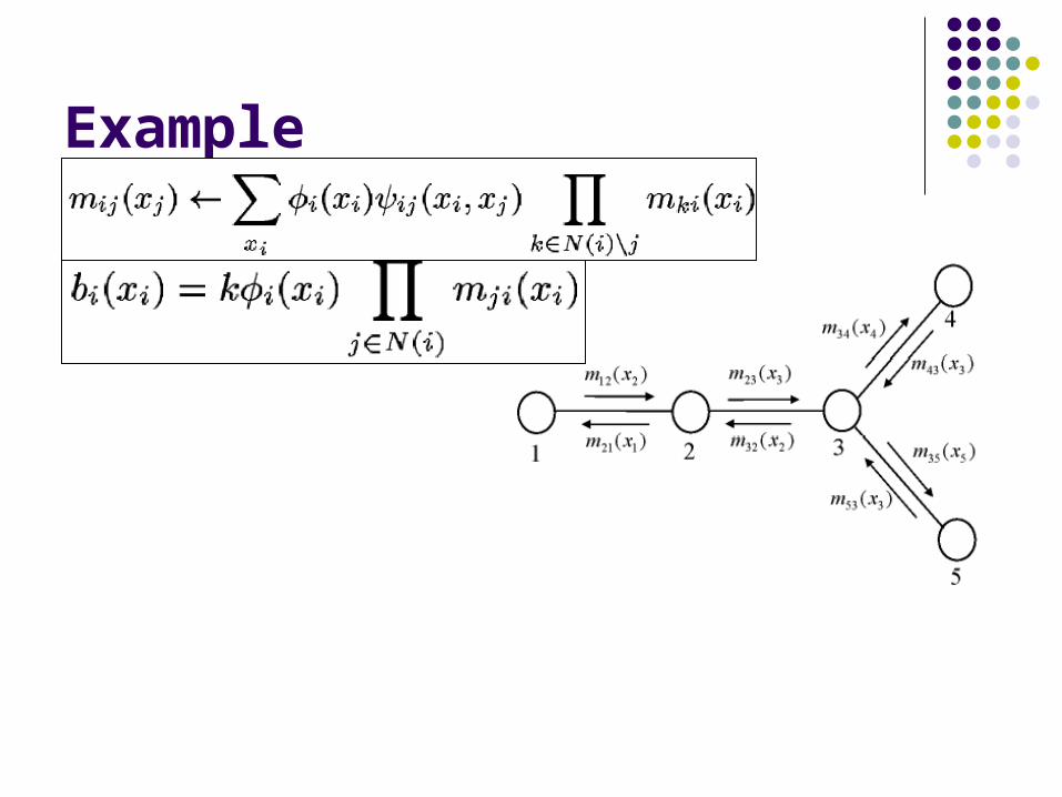
Example
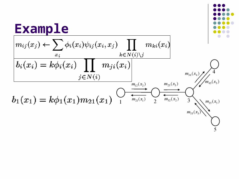
Example
Example
Example
Generalized BP
We can try to improve inference by taking into account higher-order interactions among the variables
An intuitive way to do this is to define messages that propagate between groups of nodes rather than just single nodes
This is the intuition in Generalized Belief Propagation (GPB)
GBP Algorithm
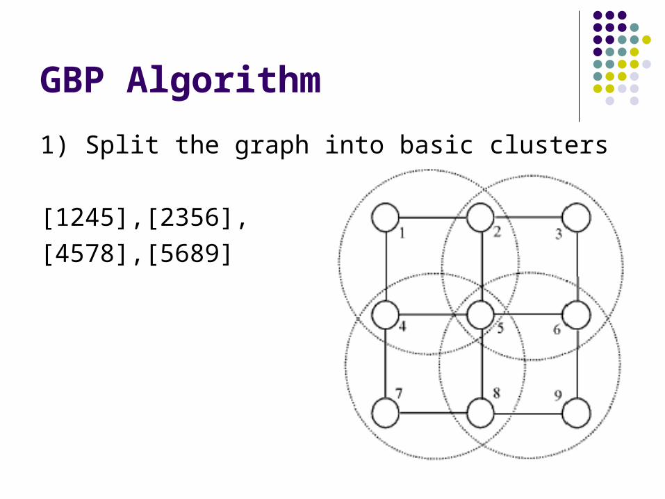
1) Split the graph into basic clusters
[1245],[2356],
[4578],[5689]
GBP Algorithm
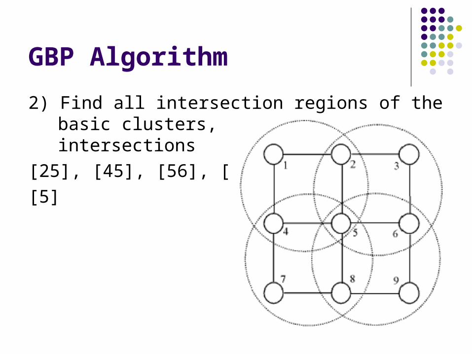
2) Find all intersection regions of the basic clusters, and all their intersections
[25], [45], [56], [58],
[5]
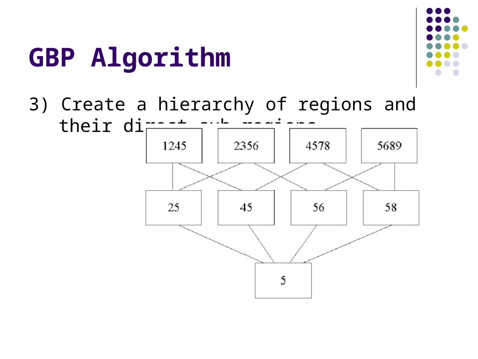
GBP Algorithm
3) Create a hierarchy of regions and their direct sub-regions
GBP Algorithm
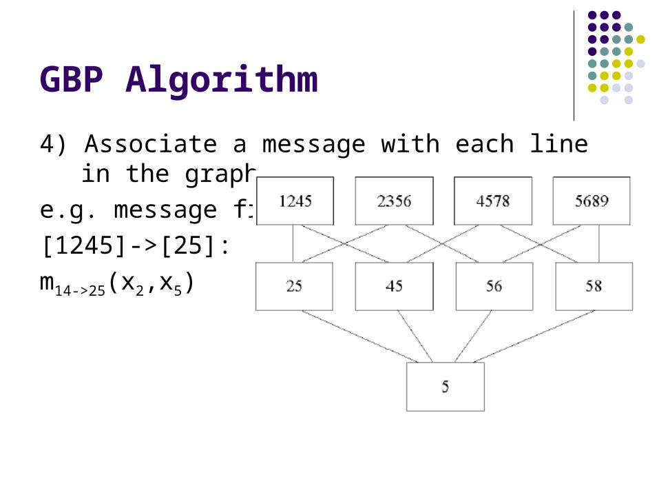
4) Associate a message with each line in the graph
e.g. message from
[1245]->[25]:
m14->25(x2,x5)
GBP Algorithm
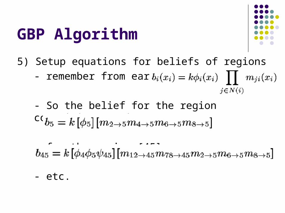
5) Setup equations for beliefs of regions
- remember from earlier:
- So the belief for the region containing [5] is:
- for the region [45]:
- etc.
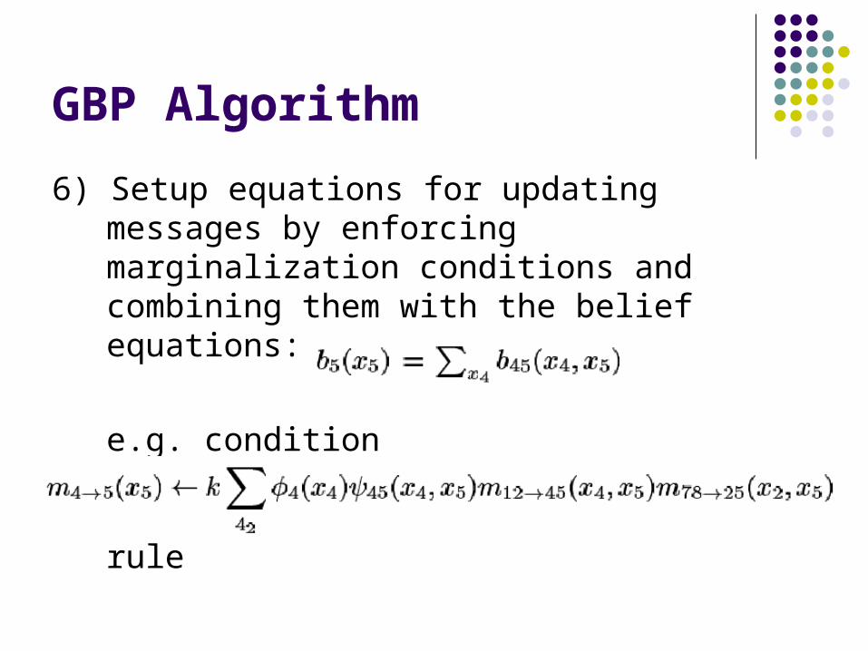
GBP Algorithm
6) Setup equations for updating messages by enforcing marginalization conditions and combining them with the belief equations:
e.g. condition yields, with the previous two belief formulas, the message update rule
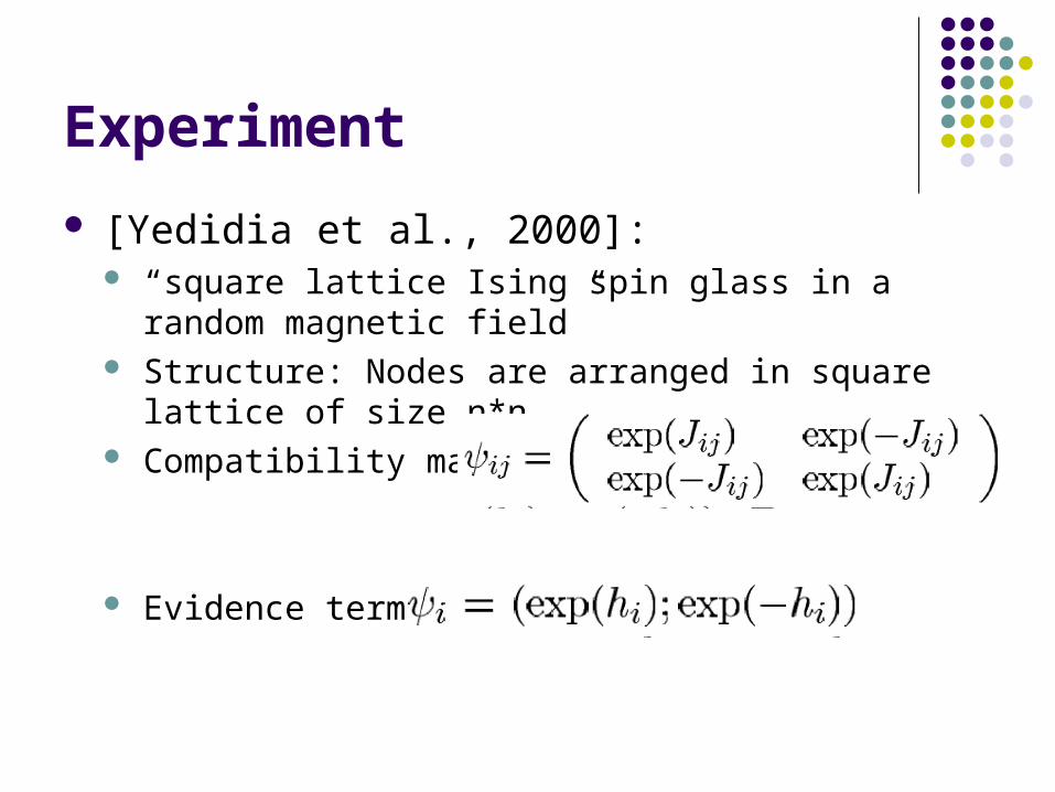
Experiment
[Yedidia et al., 2000]: “square lattice Ising spin glass in a random magnetic
field” Structure: Nodes are arranged in square lattice of size
n*n Compatibility matrix:
Evidence term:
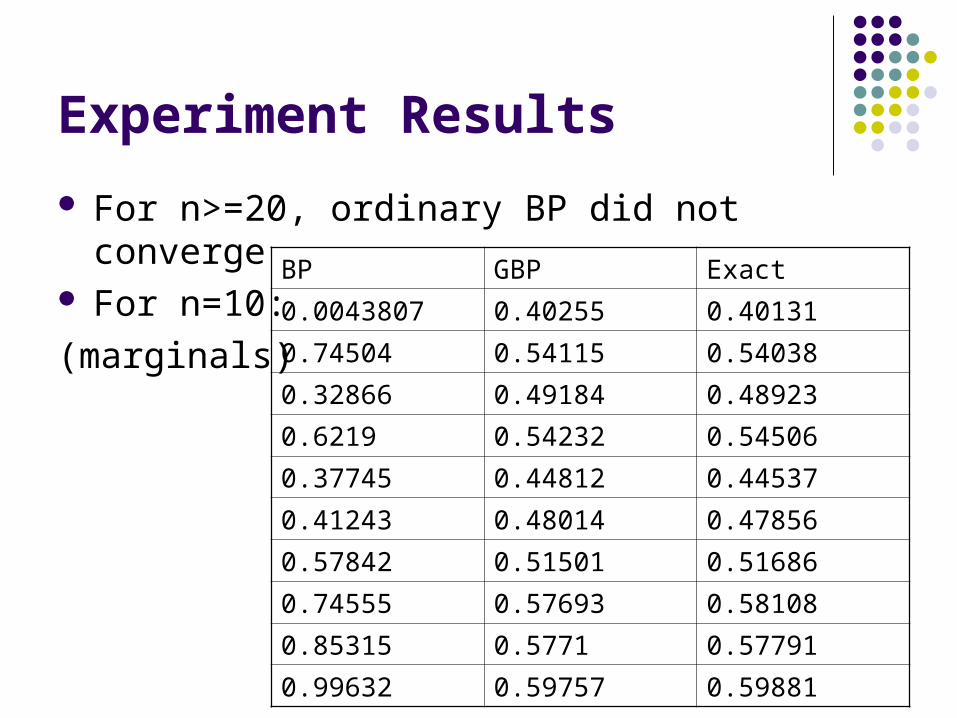
Experiment Results
For n>=20, ordinary BP did not converge For n=10:
(marginals)BP GBP Exact
0.0043807 0.40255 0.40131
0.74504 0.54115 0.54038
0.32866 0.49184 0.48923
0.6219 0.54232 0.54506
0.37745 0.44812 0.44537
0.41243 0.48014 0.47856
0.57842 0.51501 0.51686
0.74555 0.57693 0.58108
0.85315 0.5771 0.57791
0.99632 0.59757 0.59881
Outline
Motivation Pearl’s BP Algorithm Turbo Codes Generalized Belief Propagation
Free Energies

Free Energies