Embed Size (px)
Citation preview

0
—
Kaiela (Lower Goulburn River) Environmental Flows Study Final Report 24 November 2020
Dr Avril Horne, A Prof Angus Webb, Dr Libby Rumpff Meghan Mussehl, Dr Keirnan Fowler, Andrew John

1
Executive summary The Kaiela (Lower Goulburn River) is the major Victorian tributary of the Murray-Darling Basin. Over the last fifteen years, entitlements of environmental water have risen from almost zero to some 360 GL. The last environmental flow assessment was completed for the lower Goulburn River in 2011. With considerable monitoring and research undertaken in the river over the last decade, coupled with increasing environmental water allocations, an update of environmental flow recommendations was due.
In setting the terms of reference for this environmental flows assessment, the Goulburn Broken Catchment Management Authority requested that the study consider the future risks of climate change and the ecological impacts of unseasonal summer flows primarily associated with Inter-Valley Transfers (IVTs) of trade water through the Kaiela and into the Murray. They also requested a far greater emphasis on stakeholder engagement, particularly indigenous engagement, compared to past environmental flow assessments in Victoria.
The context of environmental water management in the Kaiela is continually changing (e.g. climate change, water demand and operations, scientific knowledge, community values). This project has adopted a method that recognises this continual change and the need for adaptive management, setting up an approach that allows adaptive implementation of the recommendations and ongoing revision of the technical inputs as new data becomes available. Rather than set and forget, this project sees environmental flow recommendations, and the tools that inform them, as requiring continual development, refinement and discussion.
Method
The approach adopted in this project shifts away from the commonly used Natural Flows Paradigm and instead adopts a designer flow approach. This recognises that the system is non-stationary and highly regulated, and builds the flow recommendations based on a bottom-up approach that links flows to specific management objectives. Perhaps a key example of this is that rather than use pre-determine flow components commonly used through the FLOWS method, the final flow components are identified through the development of conceptual models that link flows to specific objectives.
The project is built around a series of workshops that build a collaborative approach by bringing together local perspectives with science and water resource managers (Figure E.1). The untimely interruption of COVID-19 from March 2020 onward reduced the amount of stakeholder involvement relative to what was originally planned. Nevertheless, this study sets a new benchmark for stakeholder engagement for environmental flows assessments in Victoria. A prime example of the criticality of engagement was demonstrated in the first workshop where the community stakeholders unanimously agreed that inclusion of the floodplain was critical for the project. This required a change in project scope as the GB CMA had specified only consideration of in-channel objectives due to operational constraints and current Victorian government policies around inundation of private land..
An initial workshop with stakeholders identified objectives for environmental water. These objectives were divided into fundamental objectives, means objectives (those outcomes that support the things we fundamentally care about) and process objectives (the objectives for how decision get made and communicated). The fundamental objectives, along with a number of the key means objectives, were then incorporated into conceptual models, again using a workshop based approach. These conceptual models provide a clear link between flow components and each identified objective. They are not complete and detailed conceptual models, but rather aim to provide the key concepts that would alter flow related decision making. The conceptual models were then refined through decisions with the technical panel.

2
A structured and rigorous expert elicitation process was then used to translate these conceptual models into quantitative ecological response models. This was done through a series of questions to elicit information about the relationship between flows and ecological outcomes within the conceptual models. It is a more onerous process for a technical panel than the traditional FLOWS method and in many instances asks questions of the technical panel outside their comfort zone. In eliciting the information for the models this way, we also gain insight into the level of confidence, certainty and consistency between technical panel members. The ecological models were then presented to the technical panel and discussed, with a number of re-elicitation steps where fundamental issues were identified in the model structure. There was a relatively high level of consistency in the information elicited between experts, and with monitoring data available.
These quantitative ecological models essentially form a documented hypothesis of how the objectives will respond to flow. Their purpose is to highlight the relative benefit of different flow delivery options for environmental water, rather than to predict a specific outcome. They should be used by the CMA as working models to show the logic that links flow to outcomes, and updated as our understanding of the system changes through time (the hypothesis is updated). The combination of the ecological models and the flow tool are there to help inform and guide decision-making. They do not take away the need for discussion, debate and interpretation by the CMA in developing seasonal watering plans and deciding on individual watering events.
A set of flow recommendations was developed from a scientific expert panel workshop and interpretation of the ecological response models. The flow recommendations and ecological models were then incorporated into a bespoke flow scenario tool that will allow managers in the Goulburn-Broken catchment to test the predicted effects to ecological condition from different proposed flow regimes and environmental water use.
Figure E.. Overview of project approach
Objectives

3
Four overarching objectives were identified through the stakeholder-driven workshop process:
Maximise native floral biodiversity
Maximise native faunal biodiversity
Maximise self-sustaining populations of iconic faunal species
Promote community health and wellbeing through connection to river
These are represented through the following fundamental objectives that can be monitored, modelled and planned for through the environmental flows program:
Maximise self-sustaining populations of native large bodied fish
Maximise self-sustaining populations of native small bodied fish
Maximise self-sustaining populations of floodplain birds
Maximise self-sustaining populations of turtles
Maximise self-sustaining populations of platypus
Maximise structural complexity and diversity of floodplain vegetation, including wetlands
Maximise structural complexity and diversity of bank vegetation
Ensure social and community needs of the river are met (including fishing, boating, swimming and ceremonial uses)
Traditional environmental flow studies would often include water quality, geomorphology and macroinvertebrates within the objectives. These were not identified as fundamental objectives by the community, however they were identified as means objectives (i.e. essential for achieving the fundamental objectives). In the flow recommendations and ecological model outputs it is clear that supporting geomorphology and macroinvertebrates is essential in achieving the fundamental objectives identified by stakeholders.
Flow recommendations
A summary of the flow recommendations is provided in Table E.1. Unlike previous flow recommendations, these are provided as a list in order of priority for delivery. There was substantial discussion at the workshops around what factors might change priority for delivery (for example a wet or dry year) and it was decided that a wet year would allow more flow components to be delivered, however the priority of the flow components would not change. The most important flow component to deliver is variable baseflows year round. During summer and autumn, these baseflows are to be varied between 500-1000 ML/d during the summer and autumn months, however in winter and spring the volume has no upper limit. The second most important flow component is a winter flow event that at least partially inundates the floodplain of the Kaiela. This highlights the importance of channel formation for a number of the fundamental objectives. Other flow recommendations are summarised in the table below. It is important to note that there are additional considerations and trade-offs provided with the recommendations in Table 24 of the full report, and these should be consulted to provide all relevant information. An important element of involving the community in the flows study is the considerations for delivering environmental water that relate to community use of the river.
There are a number of risks or challenges identified to delivering environmental flows and meeting the identified objectives. These include risks from river operations, risks from climate change, the challenges of an interconnected system and of capacity constraints. The two issues consistently raised by community

4
members that they would like addressed in future are the high summer flows caused by IVTs, and the current lack of floodplain inundation.
The study identified that while the Kaiela is vulnerable to climate change impacts on water supply, it will be relatively less affected that other nearby rivers, and therefore may be subject to even greater demand for reliable consumptive water in future. However, climate change will reduce managers’ ability to deliver some of the higher-magnitude recommended flow events as these rely on piggy-backing upon natural flow events.
Transfer of traded water in the form of IVTs will remain an issue for flow management in the Kaiela into the future. The way IVTs are currently delivered as unnatural high flows over summer, delivered at short notice, but with caps on peak flows, makes it very difficult to minimize environmental damage, and also reduces achievable ecological outcomes from environmental water delivery.

0
Table E.1: Summary of environmental flow recommendations (refer to Table 10 for complete recommendations)
PRIORITY FLOW COMPONENT MAGNITUDE DURATION TIMING FREQUENCY RELEVANT OBJECTIVES
1 Year round Baseflow
(Providing habit diversity and sustaining the
system)
Preferred flows are between 500 – 1000 ML/d (or natural) during summer and autumn
During summer and autumn, ensure variability in flow regime (CV > 0.2) (e.g. mean of 750 and standard deviation of 150 ML/d)
During winter and spring ensure flow is great than 500 ML/d
N/A Year round
Every Year All Fish, Instream Productivity Macroinvertebrates Littoral Vegetation, Midbank Vegetation- Bank Stability, Turtles, Social
2a Overbank or high flows
(channel forming event)
Opportunistic event – aim to provide as high as possible an event by piggybacking natural event. Where overbank not possible, still provide as large an event as possible (aiming for 15,000 ML/d) for channel maintenance and forming.
>30,000 ML/d allow significant area of floodplain vegetation to be inundated
>20,000 ML/d inundates floodplain near Loch Garry >10,500 ML/d starts to inundate low lying
floodrunners and anabranches
Areas on the lower floodplain will fill instantaneously.
5 days at peak to fill
larger wetlands (base this on opportunity to piggyback).
Ideally late winter to spring or as naturally induced
Not during
summer to minimize black water events.
As often as possible given natural flow events
Aim for an event >10,500 each year (rainfall runoff or release)
>20,000 7 in 10 years or as per natural rainfall runoff
>30,000 Natural frequency.
Opportunistic Fish Periodic/Equilibrium Fish Instream Productivity Macroinvertebrates Littoral/Bank Vegetation Floodplain Vegetation Instream Habitat Complexity Turtles, Platypus
2b Early Spring fresh (Priming the
system)
(Provide if 2a not achievable or if 2a occurred early in winter allowing a second fresh)
Range 5,000 ML/d to 10,500 ML/d >5000 ML/d provide some benefit for bank
vegetation >7300 ML/d to mobilize bed sediments and scour
fine sediment
7 days at peak At least one annually in
early spring
Yearly All Fish Macroinvertebrates Littoral/Bank Vegetation Instream Habitat Complexity
4 Autumn fresh (flow variability and
ecosystem maintenance)
>5700 ML/d to reset surfaces
1 – 2 day at peak for vegetation and scouring
7 days at peak for migration of fish
During the growing season
Yearly All Fish Macroinvertebrates Littoral/Bank Vegetation Instream Habitat Complexity
5 Late Spring fresh (to cue fish spawning)
>7,500 ML/d for high chance of spawning >5600 ML/d for any benefit
2 day at peak Nov – Dec when Water temperature > 19°C
Yearly Periodic Fish Macroinvertebrates Instream Habitat Complexity
6 Winter-Spring variable baseflow
(Ensure habitat diversity)
Variability required – mimic natural variability by passing freshes and larger events from tributaries
>500 ML/d - natural
N.A Winter/spring Yearly All Fish Macroinvertebrates Littoral Vegetation Midbank Vegetation Instream Habitat Complexity

0
Recommendations for further work
Overall, the new recommendations, coupled with the flow management tool, should provide managers in the Goulburn-Broken catchment the ability to plan flows at annual and multi-annual scales. Moreover, these tools are designed to be used within an adaptive management framework that uses new monitoring data to continually improve the models’ abilities to predict, and thus inform, the improved management of environmental water in the Kaiela.
This project has led to the following recommendations for future activities to support environmental water management
1. Traditional Owner engagement - There is real potential to enhance environmental water management through engagement with the Yorta Yorta Nation, where possible looking for mutual outcomes by making links to cultural flows and integrating their knowledge and understanding of country.
2. Model reviews and link to monitoring and data collection - To remain relevant, it is important that the ecological models are updated overtime with new knowledge. One way to do this is to link the models to monitoring and data collection and gradually refine the models to become more data dependent.
3. Further investigation of options to deliver flows onto the floodplain - Further investigations into the implications of climate change that specifically address impacts on high flow events should be undertaken prior to inform decisions around how best to reengage the floodplain.
4. Targeted monitoring and investigations to better understanding of role of winter and spring flows - Winter and spring base flows appear low in the priority list and play only small roles in the ecological models. We recommend specific research and investigation of the role of winter and spring baseflows and the implications for each of the objectives.
5. Role of bank stability in overall geomorphic complexity - The flows scenario tool output highlighted an apparent incongruity between the bank stability model and the geomorphic complexity model. Put simply, IVT flows had clear negative impacts on bank stability but little apparent impact on geomorphic complexity. It could be that the different way in which bank stability was incorporated into the geomorphic complexity model has reduced the actual importance of this process in predictions of geomorphic complexity. Given that IVTs are likely to continue to be an important part of the water management landscape in the Kaiela, resolving these uncertainties is of high priority
6. Exploration of role of Goulburn Environmental Flows and Goulburn system to delivery of Murray River environmental and consumptive objectives (IVTs)
Although the flow recommendations reported here have greater consideration of the effects of unseasonal summer flows, they do not attempt to answer the specific question of how to deliver consumptive and environmental water to the Murray River through the Kaiela. Opportunities should be explored such that flow management may be optimized to allow for simultaneous consumptive and environmental outcomes.
7. Consideration of the role of the Goulburn River within the Basin - There is also a role for the Goulburn River in contributing to downstream values and health of the Basin and this role requires further consideration in implementing the flow recommendations.

1
Table of Contents
Executive summary .......................................................................................................... 1
1 Introduction ............................................................................................................... 3 1.1. Background ....................................................................................................................... 3
1.2. Project Objectives and approach ..................................................................................... 3
2 Study Area ................................................................................................................. 5 2.1 Traditional Owners ........................................................................................................... 5
2.2 Water resource management........................................................................................... 7
2.3 Current environmental flows program, ecological values and condition ........................ 9
3 Risks and vulnerabilities ........................................................................................... 19 3.1 Introduction .................................................................................................................... 19
3.2 Risks from river operations ............................................................................................. 19
3.3 Risks from climate change .............................................................................................. 23
3.4 Challenges aligning upstream and downstream environmental demands .................... 28
3.5 Challenges from Capacity constraints ............................................................................ 29
4 Setting environmental flow objectives ...................................................................... 31 4.1 Stakeholder led objectives .............................................................................................. 31
4.2 Establishing a hierarchy of objectives ............................................................................ 32
4.3 Objectives for the Kaiela ................................................................................................. 32
4.4 Process objectives ........................................................................................................... 38
5 Development of ecological models to support decision making ................................ 40 5.1 Method ........................................................................................................................... 40
5.2 Summary of flow needs based on ecological models..................................................... 44
5.3 Monitoring and data integration .................................................................................... 47
6 Flow Scenario testing to inform flow recommendations ........................................... 52 6.1 Flow scenario tool ........................................................................................................... 52
6.2 Flow scenarios................................................................................................................. 53
6.3 Results ............................................................................................................................. 53
6.4 Comparison to data ........................................................................................................ 58
6.5 Summary ......................................................................................................................... 60
7 Determining environmental flow recommendations ................................................. 62 7.1 Overview of approach..................................................................................................... 62

2
7.2 Environmental Flow Recommendations......................................................................... 62
7.3 Linking the flow recommendations to the ecological model and flow tool ................... 66
7.4 Potential implications of climate change ....................................................................... 69
8 Recommendations for future activities to inform environmental flows in the Kaiela . 76
9 References ............................................................................................................... 78
Appendix A: Workshop 1 Summary – Setting objectives ................................................. 81 Introductory Interview Questions ............................................................................................ 81
Workshop 1 Runsheet .............................................................................................................. 81
List of Participants .................................................................................................................... 84
Summary of objectives defined in workshop .......................................................................... 85
Notes from workshop .............................................................................................................. 91
Appendix B: Mapping previous flows studies and recommendations to stakeholder set objectives ...................................................................................................................... 97
Appendix C: Workshop 2 Stakeholder development of conceptual models ................... 105 Kaiela (Lower Goulburn) River Environmental Flows Study .................................................. 105
Model Development from Workshop 2 to final Netica Model Structures ............................ 109
Relevant flow components and existing knowledge provided to experts during expert elicitation ...................................................................................................................... 129
Appendix D: Ecological models .............................................................................................. 139
Appendix E: Workshop 3 setting environmental flow recommendations and priorities . 182 Workshop running sheet ....................................................................................................... 182
Appendix F: Flow components and considerations raised at flow recommendation stage .................................................................................................................................... 192
Appendix G: Method notes for climate change hydrology ............................................. 195

3
1 Introduction
1.1. Background
It is a critical time for the management of the Lower Goulburn River. Knowledge of the river ecosystem is greater than ever thanks to strong monitoring programs and engagement between researchers and managers. There is also a substantial volume of environmental water available to manage to achieve real ecological outcomes. However, there are challenges, both existing and emerging. The Goulburn River has seen, and will continue to see, significant changes due to system operation, irrigation demands and trade, catchment processes and climate change. Operational constraints are such that some environmental watering objectives, such as connectivity with the floodplain, are not currently achievable. Decisions around the timing, duration and volume of environmental flows are contested due to competing demands from intervalley transfers. Against a backdrop of uncertainty around the future scarcity of water and related ecological impacts of climatic change, there is real concern that these demands will result in adverse ecological outcomes. A significant challenge exists for the GBCMA to manage environmental water under these changing conditions.
At the same time, scarce water resources mean increasing scrutiny of environmental water programs and an increased awareness of the importance of community and stakeholder engagement in decision-making. It is critical that knowledge and decisions around management of environmental water is accessible and transparent. Better communication and inclusion can help ensure decisions capture values of the community and stakeholders, foster multidirectional learning, and bring a sense of ownership.
To this end, the Goulburn Broken Catchment Management Authority (GBCMA) has commissioned an environmental flows assessment for the Kaiela (Lower Goulburn) River that
i) incorporates some clear guidance around the risks of climate change and intervalley transfers to ecological outcomes, enabling the GBCMA to tackle these changing conditions (and those we have not yet foreseen), and;
ii) involves a participatory process that incorporates the ecological, social and economic benefits as envisaged by a range of stakeholders, and fosters sharing of information to develop a series of evidence based flow recommendations that meet those objectives.
1.2. Project Objectives and approach The Kaiela (Lower Goulburn) River has a long history of environmental flows, a strong monitoring program and deep scientific engagement, along with an active and engaged local community that values the river. The key challenge for this environmental flows assessment (hereafter ‘flows study’) is making use of the breadth of existing knowledge and using a participatory approach to link this knowledge with community values and experience.
The project is built around a series of workshops that build a collaborative approach by bringing together local perspectives with science and water resource managers (see Figure 1 for method overview). These workshops will be used to develop
clear objectives for environmental water in the Kaiela (Lower Goulburn) River;
models that relate water management decisions and flow regimes to outcomes for each objective;
tools to explore future scenarios, risks and key vulnerabilities; and
an adaptive management approach.

4
The project will deliver environmental flow recommendations targeting improved decision making. The CMA needs new tools and practices to provide more agile responses to future challenges. Importantly, the project also aims to build a lasting collaboration between local stakeholders, Traditional Owners, scientists and government agencies interested in the ongoing sustainability of the Kaiela.
Figure 1. Overview of project approach
The approach adopted in this project shifts away from the commonly used Natural Flows Paradigm (Poff et al., 1997) and instead adopts a designer flow approach (Acreman et al., 2014, Poff, 2018). This recognises that the system is non-stationary and highly regulated, and builds the flow recommendations based on a bottom-up approach that links flows to specific management objectives. In contrast, natural flow paradigm influenced approaches pre-determine particular flow components that are expected to be widely ecologically relevant.

5
2 Study Area The Kaiela (Lower Goulburn) River is the stretch of river downstream of the Goulburn Weir to the confluence of the Murray River, including the associated floodplains. The CMA has divided the Kaiela into two reaches for management purposes (see Figure 2):
4. Goulburn Weir to Loch Garry (110km); and
5. Loch Gary to the Murray River (125km).
While the Kaiela is the focus of this study, it cannot be discussed in isolation of the Goulburn River as a whole and the management of upstream reaches, in particular the Warring (Mid Goulburn River) which is the river between Lake Eildon and Goulburn Weir. This section introduces the study area including the Traditional Owners, current river operation and water uses, and current environmental water management and objectives.
Figure 2. Map of study area
2.1 Traditional Owners The Yorta Yorta Nation extends either side of the Murray River, and includes the riverine plains of the Goulburn Broken Catchment, including the junction of the Goulburn and Murray Rivers (Figure 3). Yorta Yorta people know the Lower Goulburn River as the Kaiela, meaning father water. The Yorta Yorta Nation is neighboured by Taungurung Country which includes the high country areas of the Goulburn Broken Catchment, including the head waters of the Goulburn and Broken Rivers. The Warring (Mid Goulburn River) is significantly impacted by the operation of Lake Eildon.
In 2007, MLDRIN released the Echuca Declaration, which defined cultural flows as:
“water entitlements that are legally and beneficially owned by Aboriginal Nations of a sufficient and adequate quantity and quality to improve the spiritual, cultural, environmental, social and economic conditions of those Aboriginal Nations. This is our inherent right.”

6
In 2016, the Water for Victoria policy document required water planners to ensure greater Aboriginal participation in water planning and management, as well as to better recognise the importance of Aboriginal water values and water rights to support Aboriginal economic development (Department of Environment Land Water and Planning (Vic), 2016). This overarching policy commitment has since been reflected in the Minister for Water’s letter of expectations to all water corporations each year. DELWP has also provided significant funding to Aboriginal organisations to complete ‘Aboriginal Waterways Assessments’, which include both environmental and cultural values (Mooney and Cullen, 2019).
An Aboriginal Waterways Assessment has not yet been undertaken for the Kaiela, nor are any cultural flows held through the Goulburn River system. However, a Whole of Country Plan (Yorta Yorta Nation Aboriginal Corporation, 2012) has been written. The plan highlights that the “Yorta Yorta see no separation between cultural and natural resources; or between Yorta Yorta people and their Country.”
“For Yorta Yorta people, the land and the world view in which they live is an extension of themselves. The land and water is the embodiment of their identity and existence, as river based people, passed on by the great creation spirit Biami” (Dr Wayne Atkinson)
It also highlights that Yorta Yorta people see their country as a whole and recognize the inherent links between land and water management—two aspects that have traditionally been separated in European natural resource management.
The Whole of Country Plan identifies an action platform, with 3 actions that relate directly to this flows project (and others indirectly):
Manage endangered and threatened flora, fauna, species and habitats
“Of particular concern is the health and status of the turtle populations. Turtles are important to the Yorta Yorta as both a totemic protector and as a food source. Bayadherra, the Broad-shelled Turtle Chelodina expansa, is a totem species and plays a significant role in Yorta Yorta creation stories, acting as a provider, guide and protector. The two other turtle species, Dhungalla Watjerrupna, the Murray River Turtle Emydura macquarii, and Djirrungana Wanurra Watjerrupna, the Common Long-necked Turtle Chelodina longicollis, are culturally significant as a food source.”
Improve water quality and water flows, and wetlands restoration
“This drastic fall in discharge resulted in the drying of most floodplain habitats and the death of many of the River Red Gum Trees that grow on the floodplain. Flooding and water flows have changed in timing and now peak during the summer irrigation season (Close 1990) This has had major consequences for the health of reptiles including turtles, and has required both Yorta Yorta and other natural resource managers to adapt our management practices and priorities, including in relation to uses and quality of water resources.”
Investigate Yorta Yorta’s role and opportunities for engagement in climate change research, programs, services and investments
“Yorta Yorta also seeks an active role in the design and construction of biodiversity corridors across Yorta Yorta Country in collaboration with the range of land and water managers responsible for landscape health and healing, and reducing carbon impacts.”
The Yorta Yorta people are represented on the Steering Committee for the flows project and were asked to participate in all workshops and through other forums.

7
Figure 3. Map of Yorta Yorta Nation
2.2 Water resource management Flows in the Kaiela have been significantly altered by the construction and operation of upstream Lake Eildon and Goulburn Weir. Lake Eildon harvests significant volumes of water during wetter months and regulates releases to meet irrigation and other consumptive demands during dry periods and summer months. Goulburn-Murray Water (GMW) operates the infrastructure to deliver water to meet consumptive demands, with Goulburn Weir diverting a significant volume of flow though the Waranga, Stuart Murray and East Goulburn Main channels to meet water needs in key Goulburn-Murray irrigation districts, the lower Campaspe and lower Loddon rivers. Several unregulated tributaries including the Acheron, Taggerty and Yea Rivers add some flow variation downstream of Lake Eildon. Tributaries downstream of Goulburn Weir, in particular the Broken River and Seven Creeks add flow variation on top of the regulated flow regime in the Kaiela.
Under the current Bulk Entitlement (BE) there is a minimum flow requirement in the Goulburn River immediately downstream of Goulburn Weir of a weekly average flow of 250 ML/d and minimum flow on any one day of 200 ML/d. Releases from Goulburn Weir may also be driven by the need to meet minimum flow
Consideration within project: In keeping with the Yorta Yorta Whole of Country Plan, we recognise the importance of including the Yorta Yorta people in decision making processes around management for the river. There was early representation on the Steering committee, however staffing changes throughout the project led to a loss of continuity.
It was not possible to complete a cultural flows assessment within the scope of this project. However, we recommend that this is discussed with Yorta Yorta Nation Aboriginal Corporation in the future and where appropriate, the environmental flow recommendations are adapted.

8
requirements when there are low tributary inflows and no other passing flow requirement at McCoys Bridge. Passing flow requirements at McCoys Bridge are:
(i) average monthly minimum of 350 ML/d for the months of November to June inclusive, at a daily rate of no less than 300 ML/d; and
(ii) average monthly minimum of 400 ML/d for the months of July to October inclusive, at a daily rate of no less than 350 ML/d.
The floodplain of the Kaiela is now predominately used for agriculture, a large portion of which is within the boundaries of the Goulburn-Murray Irrigation District. Over the last twenty years the GMID has had a net decline in usage of 1,000GL/y (almost 50%), with half of this due to the Basin Plan recovery of entitlements and the other 500GL/y due to water trade, climate, carryover, new reserve policies and earlier water recovery initiatives such as The Living Murray (RMCG, 2018). The types of enterprises using water in the region have changed and will continue to do so (see Table 1). The dairy industry in the Goulburn irrigation region has already reduced production levels by one third of pre-millennium drought levels. This is expected to reduce further in the future.
Table 1. Water use in the GMID by sector (GL, including 70 – 120 GL groundwater) (Source: RMCG, 2018)
Sector 2000 Current 5 years time 5 years time with 450 GL UpWater*
Average Average (17/18)
Last drought (06/07)
Average Drought Average Drought
Mixed Grazing 283 139 75 110 40 85 30
Crops 160 155 42 108 34 91 29
Dairy 1468 825 615 720 359 595 300
Horticulture 90 131 100 138 137 138 133
Total 2000 1250 832 1075 570 908 491
*Basin Plan has provision for a further 450 GL of water recovery from infrastructure water saving projects. Savings in GMID has been indicated as a possible source, although this may not be practical given the extent of existing efficiency work that has occurred in the region (RMCG, 2018)
Carryover of water allocations is used significantly by irrigators to manage risk between seasons. At the start of the 17/18 season, carryover was at an all-time high of 2,000 GL (equivalent to the total volume of water used in each season of the last 3 drought years) (RMCG, 2018). The level of carryover has resulted in a reduction in average annual water use within current years.
There has been an increase in deliveries from the Goulburn Inter-Valley Trade account to the Murray system in the four two years. This is largely driven by strong trade demands from increased plantings in the Murray system, coupled with drought conditions in NSW and the relative level of security in the Goulburn system. Inter-Valley Transfers (IVTs) cause significant volumes of water to be transferred out of the Goulburn system over the irrigation season, leading to unseasonal and prolonged high summer flows downstream of Goulburn weir. Prior to 2013-14, IVT deliveries averaged in the order of 60GL. This increased to 320 GL in 2017-18 and 433 GL in 2018-19 (RMCG, 2018). In August 2019, the Victorian Government announced interim changes to the trade rules in the Goulburn system designed to reduce the amount of water being traded over the summer-autumn period (https://waterregister.vic.gov.au/about/news/274-changes-to-goulburn-system-trade-and-operational-arrangements).

9
2.3 Current environmental flows program, ecological values and condition 2.3.1 Environmental water entitlements The availability of environmental water in the Kaiela has increased dramatically over the last decade. Early environmental entitlements were established under the Victorian government’s Environmental Water Reserves initiative. However, the increasing severity of the Millennium Drought during this period meant that environmental allocations were small. Environmental allocations increased markedly following the changes to the Federal Water Act in 2007 and the advent of The Basin Plan. Through water buy backs and efficiency schemes, the amount of Commonwealth Environmental Water (CEW) has increased from an entitlement of just 1,942 ML in 2009 to 360,024 ML in 2020, with a near doubling of total entitlements occurring since 2012 (Figure 4).
Figure 4. Commonwealth Environmental Water entitlements in the Goulburn River over 12 years. Shading denotes high- and low-reliability water. Data sourced from the Commonwealth Environmental Water Office (https://www.environment.gov.au/water/cewo/about/water-holdings) and K. Webber, CEWO, pers. comm.).
Smaller environmental entitlements are held by the Victorian Environmental Water Holder (VEWH) and water is also delivered down the Goulburn for MDBA allocations under The Living Murray (TLM) program. Since 2012-13 these other environmental flows have averaged around 70 GL yearly.
0
50
100
150
200
250
300
350
400
Com
mon
wea
lth E
ntitl
men
ts (G
L)
Low
High
Consideration within project: System operation continues to change in the Goulburn system and respond to changing irrigation demands. The environmental flow recommendations need to be robust under these variable conditions.
The environmental flow recommendations have been based on the requirements for the environment not constrained by current system operation. The ability to implement the recommendations in full will require further work and discussion with GMW and others. It is not within the scope of this study to provide advice on the best delivery of IVTs. Rather, the outcomes from this project will form one input into the decisions made around how best to manage the river.

10
2.3.2 Environmental values The Goulburn-Broken Waterway Strategy (GBCMA, 2014) identifies the Goulburn River as a high priority waterway. It has significant environmental values associated with the river and its floodplain and wetland habitats. Collectively, these environments support intact River Red Gum forest and numerous threatened species such as Murray cod, trout cod, squirrel glider, and eastern great egret.
Gawne et al. (2013) documented environmental values for the Kaiela (Table 2Table 2). These confirm that the Kaiela provides considerable biodiversity, ecosystem function and water quality value.
Table 2. Ecological values of the Kaiela in relation to Basin Plan objectives and Level 2 and 3 objectives derived for the Long-Term Intervention Monitoring Project. Re-drawn from Gawne et al. (2013).
Basin Plan Level 1 objectives
Level 2 and 3 Objectives derived from the Basin Plan
Ecological values of the Goulburn River
Biodiversity Ecosystem diversity • The Goulburn River is considered a wetland of national importance, and is listed as a National Park (biodiversity values).
• The river is listed as a Heritage River in Victoria (conservation and biodiversity values).
• The river supports threatened flora and fauna species and communities (biodiversity values).
Vegetation • The river supports: o intact and generally healthy riparian and floodplain areas,
including river red gum and other ecological vegetation classes and complexes.
Invertebrates • The river supports: o a high diversity and abundance of invertebrates that are a
fundamental part of the food chain. Native Fish • The river supports:
o robust, diverse native fish populations o fish spawning and recruitment o icon species such as Murray cod and Trout cod.
Waterbirds • The river supports: o piscivorous waterbirds.
Other Vertebrates • The river supports: o frogs and turtles.
Function Connectivity • The river provides: o longitudinal connection (within the Goulburn and to Murray and
Broken river systems) o connection between channel and floodplain.
Process • The river supports: o ecosystem functions that support food chains and provide
habitat o algal primary productivity o decomposition o nutrient and carbon cycling.
Water quality characteristics
Chemical • The river provides good water quality to support the ecological values of system.
Biological • The river provides good water quality to support the ecological values of system.
Constructed levees along the Goulburn River downstream of Shepparton prevent large-scale inundation of the floodplain. Overbank flows downstream of Shepparton either return to the channel (where blocked by

11
levees), or flow north via the Deep Creek system that discharges to the Murray River downstream of Barmah. The Broken River is a major tributary of the Goulburn River, joining the Goulburn River at Shepparton.
Riparian vegetation in the Kaiela was severely impacted during the Millennium Drought. With persistent low flows in the channel during this period, terrestrial pasture grasses colonized much of the riverbank. With the drought-breaking floods in 2010-11 and 2011-12, these grasses were killed and washed away leaving the banks exposed. Also during the Millennium drought, Golden perch, a flow cued spawner, did not significantly spawn (Koster et al., 2012). This made spawning a priority for environmental flows programs to rebuild populations and age classes.
2.3.3 Targeting of environmental flows to ecological values Physical changes to the river channel and floodplain, such as levees and check banks prevent water delivery to much of the floodplain of the Kaiela, third party risks also mean that environmental flows are not delivered to achieve overbank outcomes (GBCMA, 2018). Therefore, environmental flows are targeted towards in-channel outcomes. Particular ecological objectives under existing environmental flow programs include native fish, riparian vegetation, macroinvertebrates, geomorphology, and habitat diversity (GBCMA, 2018). Under previous environmental flow assessments, these ecological values are targeted using a range of flow components (Table 3), which are then prioritised through the seasonal planning process.
Table 3. Priority environmental flow components for Kaiela for the 2018-19 water year, and determined through the seasonal watering planning process. Table modified from GBCMA (2018).
Flow Component
Ecological Value Ecological Objectives
Nested Ecological Objectives Season Reach 4 (ML/d)
Reach 5 (ML/d)
Baseflow Native fish Provide suitable in channel habitat for all life stages.
• Provide slow shallow habitat required for larvae/juvenile recruitment and adult habitat for small bodied fish
Summer Autumn Winter Spring
400 540
• Provide deep water habitat for large bodied fish
Summer Autumn Winter Spring
500 320
Baseflow Macroinvertebrates Provide food and habitat for macroinvertebrates including suitable water quality
• Entrainment of litter packs available as food/habitat source for macroinvertebrates
Summer Autumn Winter Spring
540 770
Baseflow Macroinvertebrates Provide habitat and food source for macroinvertebrates by submerging snag habitat within the euphotic zone
• Provide conditions suitable for aquatic vegetation, which provides habitat for macroinvertebrates
• Provide slackwater habitat favourable for planktonic production (food source) and habitat for macroinvertebrates
• Entrain litter packs available as food/habitat source for macroinvertebrates
• Maintain water quality suitable for macroinvertebrates
Summer Autumn Winter Spring
830 940

12
Flow Component
Ecological Value Ecological Objectives
Nested Ecological Objectives Season Reach 4 (ML/d)
Reach 5 (ML/d)
• Provision of conditions suitable for the establishment of aquatic vegetation (for macroinvertebrate habitat) Provision of slackwater habitat favourable for planktonic production (food for macroinvertebrates) and slackwater habitat
Summer (30 – 40
days)
1,500 NA
Baseflow / fresh
Geomorphology Maintain pool depth especially from unseasonal events that fill pools but do not flush them
• Maintenance of water quality suitable for macroinvertebrates
Summer <90 days
856, 1186, 1660, 2223, 3142, 4490, 6590
1096, 1505, 1993, 2711, 3800, 5240, 6060
Fresh Native fish Initiate spawning, pre-spawning migrations and recruitment of native fish (preferably late spring early summer for native fish)
• Maintain aquatic macrophytes, macroinvertebrate and fish habitat (e.g. snags) by mobilising fine sediments, replenishing slackwater habitat
Winter Spring Summer
5,600 Up to 14 days (winter/ spring) 2-4 days (summer/ autumn)
5,600 Up to 14 days (winter/ spring) 2-4 days (summer/ autumn)
Fresh Riparian vegetation Remove terrestrial vegetation and re- establish amphibious vegetation
• Provide carbon (e.g. leaf litter) to the channel, inundate bench habitats to encourage germination
Winter Spring
Summer / Autumn
6,600 ML/day 14 days (winter / spring) 2-4 days summer/ autumn 1 – 4 events
6,600 ML/day 14 days (winter / spring) 2-4 days summer/ autumn1 – 4events
Overbank Floodplain and wetland vegetation
Increase the extent and diversity of flood dependent vegetation communities
• Provide habitat for wetland specialist fish
• Exchange of food and organic material between the floodplain and channel
• Increase breeding and feeding opportunities for native fish, waterbirds and amphibians
Winter Spring
25,000 5+ days 2-3 events in a year 7-10 event years in10
NA
Overbank Floodplain and wetland vegetation higher in the landscape
Increase the extent and diversity of flood dependent vegetation communities
• Provide habitat for wetland specialist fish
• Exchange of food and organic material between the floodplain and channel
• Increase breeding and feeding opportunities for native fish, waterbirds and amphibians
Winter Spring
40,000 4+ day 1-2 events in a year 4-6 event years in 10
NA

13
Flow Component
Ecological Value Ecological Objectives
Nested Ecological Objectives Season Reach 4 (ML/d)
Reach 5 (ML/d)
Rate of flow rise
Native fish and macroinvertebrates
Reduce displacement of macroinvertebrates and small/juvenile fish
All year Max rate of 0.38 / 0.38 / 1.20 / 0.80 m river height in summer / autumn / winter / spring
NA
Rate of flow fall
Geomorphology, native fish and macroinvertebrates
Reduce bank slumping/erosion and stranding of macroinvertebrates and small/juvenile fish
All year Max rate of 0.15 / 0.15 / 0.78 / 0.72 m river height in summer / autumn / winter / spring
NA
2.3.4 Recent changes in condition: Monitoring and adaptive management Ecological condition in the Kaiela has been monitored by a wide range of programs over many years. More recently, specific responses to environmental water deliveries have been primarily monitored through the Commonwealth Government’s Long-Term Intervention Monitoring Project (LTIM; Webb et al., 2018) and the Victorian Government’s Victorian Environmental Flows Monitoring and Assessment Program (Chee et al., 2009, DELWP, 2017). VEFMAP focuses on vegetation and fish as part of a wider-scale state-wide program. The LTIM Project includes a wider range of endpoints (Figure 5), with the Goulburn River being one of seven ‘selected areas’ in the Murray-Darling Basin to assess the effects of Basin Plan environmental flows, and the only selected area in Victoria (Gawne et al., 2020).

14
Figure 5 Sites and monitoring endpoints for the LTIM Project in the Kaiela (Reproduced from Webb et al., 2019b).
The five years of the LTIM Project (2014-2019) allowed a longer-term evaluation of environmental flows. The program was able to observe repeated specific responses to environmental flow actions over time, increasing confidence in the generality of those responses, and was also able to observe general trajectories in the monitoring endpoints over the period.
It showed generally improving condition in vegetation and fish assemblages, but with specific adverse events (e.g. blackwater, IVTs) reducing condition. It also showed specific responses in physical habitat, stream metabolism and macroinvertebrate assemblages (Table 4).

15
The LTIM Project was replaced by the Monitoring, Evaluation and Research (MER; Webb et al., 2019d) Program in 2019. This will be the major monitoring project for environmental flows in the Kaiela through to at least 2022.
Table 4. Summary of observed responses to flow actions in the Kaiela LTIM Project for the four years 2014–15 to 2018–19 (Reproduced from Webb et al., 2020).
Matter Major Ecological Outcomes 2014–15 to 2018–19
Physical habitat - hydraulic habitat
• As flow increases (up to 2,000 ML/day), the area of still and slow flowing (slackwater) habitats increase. These areas are important habitat for small fish and macroinvertebrates, and are ideal sites for vegetation establishment.
• As flow increases further (to around 5,000 ML/d) the area of pool habitat for larger native fish increases.
• Adding a fresh of 5,000 ML/day to baseflow helps remove accumulated sediment from the river bed and hard surfaces such as submerged large wood habitat, greatly increasing the quality of habitats for macroinvertebrates.
• High flows that inundate benches and banks enhance sediment transport and deposition which help provide good conditions (increased soil moisture and slow flowing areas) for vegetation germination and growth.
Physical habitat – bank condition
• Current environmental flows do not cause more erosion than would occur under natural flows.
• Bank erosion and deposition are highly variable along, and up and down the banks, and over time, with a single point on the bank often changing from erosion to deposition with subsequent flow events.
• The peak flow or volume of water is not related to bank erosion.
• Slow drawdown rates can promote deposition and the development of mud drapes that encourage vegetation establishment. Fast drawdown rates can increase minor erosion. However, there is no influence of the rate of drawdown on significant erosion events (i.e. erosion > 30 mm).
• In 2018–19, following the high IVT flows, greater rates of both erosion and deposition were observed. However, the proportional change from previous years was small.
• Notching of the lower bank has been observed where high IVT flows were delivered at constant levels over summer
Turf mats - sediment
• Turf mats were effective at monitoring sediment deposition on channel features under different flow events.
• The winter and spring freshes provided around half of the sediment and seeds deposited across the turf mat monitoring. The environmental flows were the primary contributor of sediment and seeds to higher sections of the riverbank, providing three-quarters of the sediment and seed deposition on these features.
• IVT resulted in more sediment being deposited on bars rather than on higher bank features.
• Across all flow events the highest deposition occurred on bars with the lowest deposition occurring on benches and ledges.
Stream metabolism: production and respiration
• Stream metabolism (the amounts of carbon created and consumed each day) increases with increasing in-channel flows up to around 4,000 ML/d. This represents a benefit to the total food resources produced for fish and other organisms, especially at small flow increases. However, it is still suggested that larger flows that inundate flood runners and parts of the floodplain would provide even greater benefits.
• Metabolic rates are seasonal with highest rates during December–January, typical of those in the southern Murray-Darling Basin but at the lower end of the ‘normal’ range on a global comparison.
• Over the five years at McCoy’s Bridge, it was estimated that Commonwealth environmental water produced about a quarter of the organic carbon created by GPP over the five-year period. With greatest benefits in spring-time and winter when 35–73% and 60–65% respectively of all GPP was associated with the extra CEW of winter-time organic carbon load in the final three years of the LTIM project.
• Low DO as a result of summer tributary inflows of poor quality water associated with intense storm events occurred in 3 of 5 years (2014–15, 2016–17 and 2017–18), and caused an anoxic event in 2016–17 that resulted in fish kills.
Algal Biofilms Results from preliminary investigations over one-year show:
• Elevated flows (environmental or for consumptive purposes) result in reduced algal biofilm biomass on hard substrates and alterations to the relative biofilm community composition from diatom dominated to cyanobacterial and/or chlorophyte dominated. This may reduce food availability for macroinvertebrates.
• Seasonal differences are observed in biofilm abundance and composition. It is unclear if this is due to managed flows or environmental factors. Further investigation is needed to elucidate this.

16
Macro-invertebrate biomass and diversity
• Macroinvertebrate richness, abundance and large crustacean biomass increased in both the Goulburn and Broken rivers following natural winter/spring floods in 2016.
• Smaller environmental flows also resulted in increased macroinvertebrate biomass and abundance, although the effect was smaller when compared with natural events.
• Crustacean abundance and biomass generally increased in the edge habitats after the CEW suggesting complex habitats, particularly aquatic vegetation refuges are important for these species.
• The January 2016 blackwater event resulted in a decline in water quality, increasing stress, mortality, and causing macroinvertebrates to drift downstream.
• Winter flows may be important in sustaining crustacean abundance and biomass and suggests it is important to monitor multiple sites within a catchment to understand drivers of key crustacean populations.
Bankside vegetation abundance and diversity
• High flow events provide soil moisture to the banks that help plant establishment and growth.
• Early spring freshes promoted the establishment and growth of flood tolerant plants and reduced the occurrence of terrestrial plants on the banks of the Goulburn River.
• Cover and occurrence of flood tolerant vegetation has risen over the term of the LTIM Project, but appears to have reduced following high IVT flows in summer 2018–19.
• Natural flooding and spring freshes help reduce the cover of exotic pasture grass. However, prolonged natural flooding in spring 2016 also caused declines in cover and presence of some native species.
• Despite short-term increases in the cover of water dependent vegetation there has not been a sustained increase in cover of water dependant plants as a group
Turf mats - seeds • Turf mats were successful at capturing seed deposition under a range of flow events.
• Seed abundance tended to be highest on ledges and bank features.
• Darcy’s track and Loch Gary had similar rates of deposition. McCoy’s Bridge had the lowest rates of deposition.
• Winter freshes and IVT flows tended to deposit the greatest number of seeds, but the results varied amongst sites and channel features.
• More than 50,000 seedlings from 94 different taxa were successfully germinated for seeds deposited on turf mats
• More than 50 percent of seedlings were from two species of rush (Juncus usitatus, Juncus amabilis) and one sedge (Cyperus eragrostis)
• Tributary inflows may help provide sediment that enhances seedling germination, but further investigations are required to confirm this.
Native fish movement
• Golden perch undertake large-scale (e.g. 10s-100s of km) movements during the spawning season in association with high flows, including during periods of targeted managed flow releases.
• Movements occur predominantly downstream to the lower reaches of the Goulburn River, or into the Murray River, followed by a return upstream movement.
• A strong association between long-distance fish movement and the occurrence of spawning suggests reproduction is a driver of fish movement.
Native fish spawning
• Golden perch spawn in response to increases in flow and appropriate water temperature (>18.5 °C) in the lower Goulburn River, including within-channel flow pulses or bankfull flows especially around November-December, including during targeted managed flow releases (i.e. ‘freshes’).
• Silver perch spawn in response to increases in flow and appropriate water temperature (>20 °C) in the lower Goulburn River, including within-channel flow pulses or bankfull flows especially around November-December, including during periods of targeted managed flow releases.
• Silver perch eggs were also collected coinciding with an increase in flow in mid-December 2018 associated with inter-valley transfer flows.
• The collection of trout cod larvae in the last two years (2017 and 2018) across a range of sites (Pyke Road, Loch Garry, McCoy’s Bridge, Yambuna) demonstrates that breeding populations exist in the lower Goulburn River.

17
Fish communities (composition and abundance)
• The lower Goulburn River supports significant populations of native fish, including several species of conservation significance, namely Murray cod, silver perch, Murray River rainbowfish and trout cod.
• Murray Cod spawn annually in the lower Goulburn River regardless of river discharge. Natural spawning contributes substantially to the Murray cod population in the lower Goulburn River.
• Silver perch were generally collected in low numbers in the surveys, although abundance increased considerably in 2017, likely due to increased immigration following high spring flows in 2016 and managed flow releases in summer/autumn 2016–17.
• Murray River rainbowfish decreased in abundance in the last two years (2018 and 2019), potentially related to prolonged high summer flow conditions due to inter-valley transfer (IVT) flows. To better understand the potential effects of IVT flows on fish, it is recommended that a monitoring program be designed and implemented specifically for this purpose.
• Adult trout cod were not common in the surveys, but the collection of larvae in the last two years (2017 and 2018) across a range of sites (Pyke Road, Loch Garry, McCoy’s Bridge, Yambuna) demonstrates that breeding populations exist in the lower Goulburn River.
• Currently, the golden perch population in the Goulburn River consists mostly of stocked fish, although spawning in the Goulburn River and immigration of fish from the Murray River also contribute to the population. Whilst in situ recruitment is low in the Goulburn River, the Goulburn River is also a source of fish to the Murray River.
Coordination of LTIM-based monitoring with other selected areas, plus research and monitoring funded through other programs, has also shown the importance of larger-scale connection for the management of golden and silver perch. Micro-chemical analysis of otoliths from golden perch has shown that many fish in the Kaiela were hatched elsewhere in the southern Murray-Darling Basin and migrated through the connected system as young fish (Zampatti et al., 2019). A flow management experiment carried out in 2017 showed that high autumn flows in the Goulburn and Campaspe rivers, coupled with lower flows in the Murray River, could attract golden and silver perch from the Murray into the Goulburn River (Tonkin et al., 2017), potentially explaining these large-scale patterns. This type of larger-scale coordination and understanding will become more important for environmental flows planning and management into the future.
The LTIM Project also saw improved adaptive management of environmental flow decision making in the Kaiela. Through both formal (an annual stakeholder forum) and informal (phone calls and conversations between managers and researchers), results from the monitoring were able to be incorporated into decision making well ahead of the annual reporting cycle (Watts et al., 2020).
Finally, although there has been a generally improving trend in ecological condition through the five years of the LTIM Project, specific adverse events and limitations have interrupted these trajectories and will remain challenges for management going forward.
A major blackwater event occurred in the Kaiela below Shepparton in January 2017 (GBCMA, 2017). This caused fish deaths with an observed decrease in adult fish abundance in the annual fish surveys in 2018. Although beyond the control of catchment managers, this type of event will continue to impact upon positive effects of environmental flows.
The inability of river managers to deliver environmental flows to deliberately inundate the Kaiela floodplain also places limitations on the benefits possible with environmental flows. The natural flooding event that occurred in spring 2016 drove a surge in secondary production of macroinvertebrates, presumably through the introduction of significant amounts of allochthonous carbon into the river channel. Such responses have not been seen in the two monitoring seasons since then (Webb et al., 2019a), where spring freshes have peaked at around 8,000 ML/day or approximately half way up the river bank. These flows are not sufficient to engage any off-channel habitats that may contribute large amounts of carbon. The large-bodied crustaceans that were monitored are important prey species for native fish. Thus, increased inundation of the floodplain has the potential to greatly improve food webs and productivity at all trophic levels.

18
Finally, as described in more detail below, IVTs are causing damage to riverbank vegetation and increased bank erosion through prolonged inundation in summer, and may also have other ecological impacts. These events have also impacted upon the sampling schedule and efficiency for the LTIM project (Webb et al., 2019a), and although this is not an ecological impact as such, it does affect our ability to detect the effects of environmental flows.

19
3 Risks and vulnerabilities
3.1 Introduction Discussions with stakeholders identified a number of key current and future risks to the environmental condition of the river. This section briefly discusses risks from river operations, risks from climate change, the challenges of an interconnected system, and of capacity constraints.
3.2 Risks from river operations Recent years have seen substantial changes in the delivery of water down the Goulburn River in spring and summer as inter-valley transfers (IVTs). From quite low volumes of IVTs in 2014-15, volumes increased sharply in 2017-18 and even more so again in 2018-19 (Figure 6). IVTs also began much earlier in the 2018-19 water year than had been the case for previous years (Figure 6e).
0
2000
4000
6000
8000
10000
12000
14000
16000
1-Jul 1-Aug 1-Sep 1-Oct 1-Nov 1-Dec 1-Jan 1-Feb 1-Mar 1-Apr 1-May 1-Jun
Flow
rate
ML/
d
b) Goulburn River @ McCoy's Bridge 2015-16
0
2000
4000
6000
8000
10000
12000
14000
16000
1-Jul 1-Aug 1-Sep 1-Oct 1-Nov 1-Dec 1-Jan 1-Feb 1-Mar 1-Apr 1-May 1-Jun
Flow
rate
(ML/
d)
c) Goulburn River @ McCoy's Bridge 2016-1717162 23552 48729

20
Figure 6. Annual discharges in the Goulburn River at McCoys Bridge from 2014-15 (a) to 2018-19 (e). IVT components of the total discharge are depicted in red. Reproduced from Webb et al. (2019c).
These elevated flows summer are a substantial departure from historical flows. Average discharge from 1976-2010 for the period Dec-Mar is less than 600 ML/day at McCoys Bridge (Cottingham and SKM, 2011). Over the same period for 2018-19, the average discharge was 2213 ML/day at the McCoy’s Bridge gauge (http://data.water.vic.gov.au).
IVT flows are delivered under considerable constraints. The MDBA can order volumes at short notice (days), but as a total volume for the next calendar month. Simultaneously, Goulburn-Murray Water may not deliberately release more than 3000 ML/day down the Kaiela without giving riparian land holders three weeks’ notice to allow them to remove irrigation pumps or other equipment (GBCMA, 2018). The consequence of these two operating conditions is that IVT flows may be delivered at high, but relatively constant discharges, and over extended periods of time. For example, from 9/1/19 – 17/2/19, there was a 40-day period with an average discharge of 2871 ML/day and a standard deviation of just 83 ML/day (http://data.water.vic.gov.au).
Australian river systems have not evolved under conditions of elevated, constant flows and so ecological impacts from IVTs are inevitable. Cognisant of the ecological threat posed by IVTs and amid rising community concern over these potential impacts, the Goulburn Broken CMA commissioned a study in early 2019 to ascertain impacts of IVTs on bank condition and bank vegetation (Vietz et al., 2019).
The study found extensive evidence of erosion associated with the IVTs delivered over the summer period, although the erosion was not severe (e.g. no mass failures were observed). Up to 70% of the site at McCoys bridge experienced notching of the bank at two distinct heights associated with IVT flows (~ 2500 ML/d and ~1000 ML/d) and there was also bank scour below these levels (Vietz et al., 2019).
Similar results were observed anecdotally through monitoring under the LTIM Project. In Figure 7 below, a clear area of scour and notching is visible on the mid-bank, approximately at the level the IVT inundation would have covered at 2500 ML/d (scoured area above the Juncus plants).

21
Figure 7. Riverbank notching associated with the 2018-19 IVT (Yambuna Bridge, June 2019) (Image credit, Streamology Pty. Ltd.)
Vietz et al. (2019) also observed impacts on riverbank vegetation, with young plants recruiting after spring flows and measured in December, no longer visible or only visible as browned-off and presumably dead plants following the extended IVT (Figure 8).
Figure 8. Vegetation site ‘A’ at McCoys Bridge. Recruitment of vegetation on the bar in December (visible at light green) is browned off by March and seemingly absent in April. Reproduced from Vietz et al. (2019).
Data collected by Goulburn Broken CMA confirm these conclusions. Photopoints maintained by the CMA show lower bank vegetation die off following the retreat of the IVT, but conversely improved vegetation condition high on the bank when compared to the dry summer of 2015-16 (Figure 9). These contrasting results are interpretable considering the duration and extent of the IVT compared to the low flows of summer 2015-16. During 2018-19, high flows would have adversely affected lower bank vegetation through prolonged inundation, but would also have recharged bank soil moisture higher on the banks above the IVT flow or where inundation was only brief. Conversely, in 2015-16, low flows in summer maintained vegetation low on the bank through improved soil moisture, but semi-aquatic vegetation higher on the bank dried out.

22
Figure 9. changed patterns of vegetation coverage with IVT flows. In February 2016, vegetation is present at the low water margin following low summer flows, but is in poor condition higher on the bank. In contrast in March 2019, vegetation appears dead on the lower bank, but is in good condition higher on the bank (Image credit, GBCMA).
Beyond these demonstrated impacts of IVTs, impacts to other parts of the biota are also likely based on our understanding of system function.
High flows can reduce the occurrence of shallow, slow-flowing habitat near the riverbank. Hydraulic modelling has shown that a discharge of 3000 ML/d reduces the area of such habitat by approximately 30% compared to a discharge of 1000 ML/d at McCoys Bridge (Webb et al., 2019a). Shallow, slow-flowing habitats provide ‘hot spots’ for primary and secondary production in rivers (Humphries et al., 2006) and are believed to be important habitat for small bodied fish species and juveniles of larger species.
With IVTs taking place in summer after fish reproduction, elevated flows could cause impacts on nests of Murray Cod and on juvenile fish hatched during spring reproduction, as well as small-bodied species. Summer is also the peak time for primary production by plants and algae and secondary production by macroinvertebrates. The disruption of shallow-slow flowing habitats could impact on all these.

23
Data collected under the LTIM Project has demonstrated that increased flows in the warmer months will increase the overall amount of primary productivity, as larger amounts of the river channel are inundated (Webb et al., 2019b). Thus we might expect higher overall productivity under an IVT scenario with higher flows over summer. The benefit for the ecosystem, however, is likely to be limited or non-existent. Carbon fixed by pelagic (water column) primary productivity is exported from the Goulburn into the Murray. It has been hypothesized that such carbon will have benefits much further downstream in the Coorong and Lower Lakes where it can be used to underpin food chains. However, with IVT water being extracted for irrigation in the Sunraysia district, the fixed carbon will also be lost from the river.
In addition to the GBCMA project described above (Vietz et al., 2019), IVT monitoring is being explicitly considered in the Monitoring, Evaluation and Research Program (Webb et al., 2019d). Under that program, extra vegetation monitoring is being conducted at the end of the summer period to assess vegetation survival following spring growth. The bank condition monitoring has also been expanded in terms of methods used, at least partly in response to concerns over IVTs.
Importantly, the Kaiela also has significant social and economic values that are impacted by the high volumes of IVTs during summer months. The Kaiela is popular for fishing, camping and boating. The summer season is especially important for tourism and the local economy. High summer flows impact on visitations over the summer period (peak season), and erosion of bank vegetation impact on the aesthetics of the river once water levels have dropped. The high water levels pose issues for access, with sandbars covered and reduced bank stability. Fishing is also impacted by the velocity of river flows and the reduced availability of slack water habitat. The stakeholder group at workshops raised this impact on social and economic values as a key concern.
The observed and hypothesized impacts of IVTs mean that they are an issue of considerable importance for local communities on the Goulburn River, river managers, and the scientists involved in monitoring ecological responses to environmental flows. The Victorian Government has intervened, with the announcement of interim changes to the trade rules in the Goulburn system, providing greater protection for the riverine environment. Thus, the consideration and management of IVT impacts needs to be a central tenet of any comprehensive environmental flows assessment for the Goulburn River going into the future.
Consideration within project: There is significant community concern over high summer flows caused by IVTs (as raised in stakeholder workshops). The increased summer flows held at consistent levels are having a significant impact on instream vegetation and bank stability.
The project has addressed this by considering environmental flow recommendations in the context of resilience and setting an acceptable band of flow (both upper and lower recommendations) rather than just minimum flow recommendations.
3.3 Risks from climate change Climate change may potentially cause multiple changes within the Goulburn River system, such as:
1. Changes to the average amount of streamflow in the system as a whole; 2. Changes to the balance of flows between regulated and unregulated tributaries; 3. Changes to the relative reliability of Goulburn entitlements compared to other MDB rivers, which may
impact demand/trade practices and thus river operations in the Goulburn (see IVT section above); 4. Changes to the seasonality of streamflow; 5. Changes at the extremes of the flow regime (i.e. low flow events and flood events);

24
6. Changes to the incidence of multi-year wet and dry periods; and 7. Changes to temperature, which may impact riverine and riparian ecosystems.
The existing highly-variable climate will continue to be a key driver of system behaviour and ecosystem response, so discussions of future hydrology should consider aspects of both variability and change. This section summarises available scientific evidence and links this to potential issues in the Goulburn River over planning timeframes (agreed at Workshop 1 to extend as far as 20 years into the future).
The main source of information about future climate is Global Climate Models (GCMs). There are multiple GCMs maintained by different research groups globally, and each is considered a plausible representation of the climate system. Each GCM is run for multiple different hypothetical scenarios of greenhouse gas emissions, and so there is no single ‘correct’ answer when querying future climate possibilities. The GCMs themselves also have strengths and weaknesses that need to be taken into account. For this section, we use the following two sources of information:
1. The government’s “Climate Change in Australia” website (www.climatechangeinaustralia.gov.au), which compiles the outputs of a large set of GCMs, providing effective regional summaries, and giving an indication of how much the answers vary across different GCMs for climatic variables such as rainfall and temperature.
2. A set of simulations of future projections that have been compiled and run specifically for this project and the associated Australian Research Council Linkage Project (LP1701100598, Vulnerabilities for Environmental Water Outcomes in a Changing Climate, MJ Stewardson et al.). Incorporating rainfall-runoff models as well as GCMs provides information about streamflow as well as climate variables. The specifics of these simulations are described below, but it is important to note that the diagrams are based on one possible way that the future might unfold among many that are considered plausible. Steps have been taken to ensure it is as ‘representative’ as possible (Box 1), but there is considerable underlying uncertainty about future climate.
It is likely that a long-term drying trend will be evident in northern Victoria over coming decades. The “Climate Change in Australia” site indicates that most GCMs indicate a warming of 1.5 to 3 degrees by 2050. Rainfall trends vary depending on the model, but future reductions are more commonly projected than increases, particularly in winter. It is likely that this will mean less streamflow on average in the Goulburn system. The simulations undertaken for this project indicate a decline in future streamflow such that the long-term average over 2020-2050 is similar to the Millennium Drought (Figure 10).
According to these projections, the declines will not be equally spread, with a decline of 42% of flows above Eildon (from 1537 to 890 GL/yr) compared to nearly 60% (from 758 to 323 GL/yr) for the unregulated tributaries shown. Because of this, the opportunity to ‘piggy-back’ environmental water onto flows from unregulated tributaries may reduce in the future.
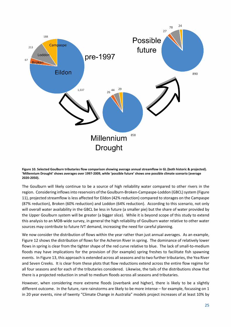
25
Figure 10. Selected Goulburn tributaries flow comparison showing average annual streamflow in GL (both historic & projected). ‘Millennium Drought’ shows averages over 1997-2009, while ‘possible future’ shows one possible climate scenario (average 2020-2050).
The Goulburn will likely continue to be a source of high reliability water compared to other rivers in the region. Considering inflows into reservoirs of the Goulburn-Broken-Campaspe-Loddon (GBCL) system (Figure 11), projected streamflow is less affected for Eildon (42% reduction) compared to storages on the Campaspe (87% reduction), Broken (60% reduction) and Loddon (64% reduction). According to this scenario, not only will overall water availability in the GBCL be less in future (a smaller pie) but the share of water provided by the Upper Goulburn system will be greater (a bigger slice). While it is beyond scope of this study to extend this analysis to an MDB-wide survey, in general the high reliability of Goulburn water relative to other water sources may contribute to future IVT demand, increasing the need for careful planning.
We now consider the distribution of flows within the year rather than just annual averages. As an example, Figure 12 shows the distribution of flows for the Acheron River in spring. The dominance of relatively lower flows in spring is clear from the tighter shape of the red curve relative to blue. The lack of small-to-medium floods may have implications for the provision of (for example) spring freshes to facilitate fish spawning events. In Figure 13, this approach is extended across all seasons and to two further tributaries, the Yea River and Seven Creeks. It is clear from these plots that flow reductions extend across the entire flow regime for all four seasons and for each of the tributaries considered. Likewise, the tails of the distributions show that there is a projected reduction in small to medium floods across all seasons and tributaries.
However, when considering more extreme floods (overbank and higher), there is likely to be a slightly different outcome. In the future, rare rainstorms are likely to be more intense – for example, focussing on 1 in 20 year events, nine of twenty “Climate Change in Australia” models project increases of at least 10% by

26
2050, increasing to seventeen of twenty for 2090. However, catchments will be drier on average due to the higher temperatures and lower rainfalls mentioned above. Because of this, small and medium floods and freshes will likely become less frequent (Figure 12, Figure 13), but more severe floods may become more common (Hirabayashi et al., 2013). Recent research by Wasko and Nathan (2019) suggests floods rarer than 1 in 10 years are the only ones that will become larger (all other floods will reduce in magnitude).
Figure 11. Comparison of flows into reservoirs in the region, showing annual average streamflow in GL (both historic & projected). The ‘Millennium Drought’ shows historic averages over 1997-2009, while ‘possible future’ shows one possible climate scenario (average over 2020-2050). “Campaspe” and “Broken” refer to inflows into lakes Eppalock and Nillahcootie, respectively. “Loddon” refers to combined inflows into Cairn Curran and Tullaroop reservoirs.

27
Figure 12. Comparing the distribution of simulated daily flows for the future (red) and the historic period (blue). This example is for the season of spring (September – November) and for the Acheron River at Taggerty (gauge 405209).
Lastly, we consider multi-year dry and wet periods. It is difficult to say if multi-year droughts will become more common because this aspect of the climate is one in which GCMs often perform poorly. When compared with historic multiyear cycles, GCM cycles may be inconsistent or sometimes entirely absent. As noted above, conditions will likely be drier on average, but variability within this long-term trend is difficult to predict. Better representation of (for example) El Nino events in models is an active area of research. Multi-year droughts like the Millennium Drought are not unprecedented in the pre-observation record (Freund et al., 2017), and so similar events may occur again within planning timeframes.

28
Figure 13. Same as Figure 12, but for all four seasons and for two further unregulated tributaries. Note, for Seven Creeks the distributions are based on the upper catchment area and do not account for flow attenuation (i.e. floods becoming smoother / less peaky) occurring between Euroa and Shepparton.
3.4 Challenges aligning upstream and downstream environmental demands The Murray Darling Basin Authority has published a Basin-wide environmental watering strategy to guide environmental water holders and managers regarding expected environmental outcomes, priorities and strategies for the Murray Darling Basin as a whole. Each year, the MDBA also identifies Basin watering
Consideration within project: To assist with developing the final flow recommendations, this project has used a number of climate change scenarios to ensure that recommendations are robust under a suite of possible futures.

29
priorities for the coming year. These system-scale priorities are considered by environmental water holders alongside local priorities for environmental water management in the Goulburn.
The Kaiela is a major tributary of the Murray, with environmental water outflows from the river (often called environmental water return flows) providing an important contribution to the health of the river and wetlands in the downstream Murray. Environmental water holders and the GBCMA aim to manage environmental water within the Kaiela in a way that meets local catchment priorities whilst also contributing to downstream environmental priorities.
It is challenging for environmental water holders to co-ordinate environmental water releases to meet both local and downstream priorities simultaneously. As an example, the ideal timing for a spring pulse for the lower Murray is generally considered to be late spring. However, over the past two seasons, the spring pulse in the Kaiela has been delivered in early-mid spring in order to provide a drying-phase for the growth and establishment of riverbank vegetation to promote resilience before either subsequent flow events (fresh for fish spawning or IVTs), or dry and hot conditions during summer. The environmental water return flows downstream from an early spring pulse in the Kaiela are still beneficial for downstream outcomes, however monitoring in the Lower Murray (through LTIM) indicates that later delivery would be preferable.
As a further example, environmental water holders often seek to provide additional environmental water to the South Australian Murray in summer and early autumn in order to maintain critical baseflows at the end of system. Baseflows of environmental water delivered in the Kaiela across summer and early autumn could help meet these demands. However, in recent seasons the Kaiela has already been running above target flow rates through summer and early autumn due to the delivery of IVTs. This has restricted the ability for environmental water to help contribute to downstream demands during the same period.
Although it can be challenging to co-ordinate the Kaiela with broader system-scale outcomes, it is nonetheless vital that water managers consider it as part of a broader river system rather than an isolated component. This is particularly important in order to achieve the objectives for native fish in the Kaiela. Monitoring has identified that a significant proportion of golden and silver perch captured in the Kaiela have spawned in the Murray and then entered the Goulburn as juveniles or adults (Zampatti et al. 2015). Improving the native fish population in the Kaiela will require designing environmental flow releases that attract and retain native fish from the Murray into the Kaiela, an approach that was trialled successfully in 2017.
3.5 Challenges from Capacity constraints Lake Eildon fully regulates downstream flows in all but very wet years. Based on a long-term average, smaller floods in the order of 25,000 ML/d occur six years in ten and larger events (40,000 ML/d) occur around three years in ten. DSE (2011) calculates that under current conditions flow events from Murchison to Shepparton of between 25,000 and 55,000 ML/d:
occur 20% to 30% less often compared to unregulated conditions;
are 50% to 70% shorter compared to their unregulated duration; and
have a maximum period between events that is 2.5 to 3.5 times longer than under unregulated conditions.
The frequency of overbank flows is now less than what is needed to maintain the health of the Kaiela floodplain and river channel (DELWP, 2016). Modelling undertaken as part of the original Business Case to
Consideration within project: Environmental flow recommendations are being made specifically for the Kaiela. This project does not adapt these recommendations to explicitly consider delivery challenges for achieving multiple benefits in the southern connected system.

30
address capacity constraints demonstrated that an average flow over 4 days of 25,000 ML/d would inundate 75% of wetlands along with key river red gum areas.
The current operational water delivery limit in stream at Shepparton is 9,500 ML/d, with a period of 1- 2 weeks notice for delivery of flows above 3,000 ML/d for most periods. Delivering these volumes of water would require “piggy backing” of unregulated river flows from the mid and lower Goulburn tributaries. There would also need to be additional capacity installed at a number of river regulators.
Under the Basin Plan, regional, state and federal authorities are investigating ways of relaxing constraints (physical and rules-based) in the Kaila river and other key points in the southern Murray-Darling Basin Authority to improve environmental outcomes. An investigation and costing has been undertaken to consider the delivery of higher in-channel flows of up to 20,000 ML/d (17,000 ML/d target with a 3,000 ML/d unregulated flow risk management buffer) in the Kaiela. To meet the 17,000 ML/d flow target, the project has investigated reducing water harvesting at Goulburn Weir (to Waranga Basin) and releasing from Lake Eildon (if necessary) to top up unregulated flows in the Kaiela (from tributary streams).
Consideration within project: The focus of this project is on flows that are within the range that might be possible based on the current business case i.e. for flows up to bankfull level, which will also allow the watering of some low lying flood runners and wetlands on the floodplain.
Many of the objectives identified by stakeholders require connection of the floodplain and wetlands through overbank flow events. Given the importance of floodplain values for the stakeholders and Traditional Owners, this project will include environmental flow recommendations aimed at achieving these objectives.
Through the flow scenario modelling exercise, we will work with the stakeholders to examine the implications of current capacity constraints in achieving these objectives. It is not the role of this project to address the capacity constraints per se (this is an key objective of the basin plan and ongoing discussion between the CMA and the Victorian Government).

31
4 Setting environmental flow objectives 4.1 Stakeholder led objectives The last decade has seen water management agencies in Victoria make commitments to collaborative and innovative catchment management strategies. The Department of Environmental, Land, Water and Planning has identified coordination between state, regional and local agencies as a target for improvement, with the aim to better align planning objectives at varying scales (DELWP, 2016). They also articulated an explicit goal of effective and equitable community engagement towards regional planning, which prompted the implementation of The Community Engagement and Partnership Framework for Victorian CMAs 1 . This framework places emphasis on embedding stakeholder and community engagement into every level of decision-making through identifying meaningful opportunities for stakeholder contributions.
Given the complex nature of river management, including the allocation and implementation of environmental flows, it is increasingly important to integrate scientific methodologies with societal values and perspectives (Poff et al, 2012). This requires agencies to place greater emphasis on designing tailored, thoughtful approaches to meaningful community engagement. Well-designed community engagement and collaborative methodologies place focus on the processes behind decision making and in doing so, build community relationships. Participatory modelling provides a tangible method for incorporating various types of stakeholders into the decision-making framework for water resources. Participatory modelling approaches draw on the diversity of stakeholder knowledge to create a shared representation of a system (Voinov et al., 2018).
The participatory modelling approach developed for this project was designed to be a collaborative process that is inclusive of multiple stakeholder perspectives and fosters multidirectional learning. The methodology is centred around a series of four participatory workshops (Figure 1). Each workshop has a unique goal that is directly tied to the identification of objectives and the development of the appropriate models. Participants were also invited to comment on all project documentation and asked for feedback at every stage. Because stakeholder participants are involved at every level of the project, their perspectives are embedded in the flow recommendations. It should be noted that this process had to be adapted as the project unfolded to account for COVID-19 restrictions.
Stakeholder identification took place through consultation with GBCMA representatives and participants can be broadly categorized into the following three groups: agency representatives, expert panel scientists, and community members. Community member participants were recruited based on further conversations with the GBCMA and focused on current members of the Environmental Water Advisory Group (EWAG). For a complete list of participants, please refer to Appendix A.
Once the list of participants was finalised, introductory phone interviews were conducted with 20 out of the 22 participants. Questions during the phone interview focused on their perceptions of environmental flows and the associated challenges in the Kaiela. Additional questions targeted participant’s views and values regarding community engagement for this project. For a complete list of interview questions, please see Appendix A. The results of these interviews were used to formulate problem statements and provide context for the first workshop.
The first workshop aimed specifically to define objectives for environmental water in the Kaiela. A key learning from the first workshop demonstrated the importance of consultation when the stakeholders unanimously agreed that inclusion of the floodplain was critical for the project. This required a change in
1 https://www.gbcma.vic.gov.au/downloads/CatchmentEconomy/CMA_Community_Engagement_and_Partnerships_Framework_Final_-_Endorsed.pdf

32
project scope as the GB CMA had specified the tender scope to only include consideration of in-channel objectives due to operational constraints and Victorian government policies of not flooding private land without consent. The process of asking stakeholders what they value from the River and what the key objectives for environmental water should be highlighted the importance of the floodplain for the community and their vision for the River. The details of the workshop structure and summary of discussion can be seen in Appendix A.
4.2 Establishing a hierarchy of objectives We focused on eliciting a first cut of the objectives specific to the management of environmental water and associated decisions around flow regime, and developing a hierarchy of different types of objectives. In a decision framework, objectives are defined as specific, measurable statements that describe what is to be achieved or avoided with management. Objectives are values focused, because they capture what we care about (e.g. fish, platypus, wetlands), but provide more detail about how we want to manage those values (i.e. minimise risk to, maximise the viability of, etc).
Different types of objectives can be identified, but decisions should be focused on those objectives that are fundamental, or the primary reason for the decision. In a hierarchy of objectives, these sit at the top. These are differentiated from means objectives (which specify the means to achieving the fundamental objectives), process objectives (which specify the way a decision might be made) and strategic objectives (which are strategic priorities of the organisation that govern all decisions, and may be fundamental to all decisions). In the development of an objectives hierarchy, we focused on presenting the fundamental (which may include strategic objectives) and means objectives. The process objectives are presented later in this report, as they provide understanding and direction for including what is important to stakeholders in the development of flow recommendations.
4.3 Objectives for the Kaiela Four overarching objectives for the Kaiela were identified through the workshop process:
Maximise native floral biodiversity
Maximise native faunal biodiversity
Maximise self-sustaining populations of icon faunal species
Promote community health and wellbeing through connection to river
These four overarching objectives were broken down into specific fundamental objectives and the means objectives to achieve these (Table 5). A first cut of objectives was developed during the stakeholder workshop. The means objectives were then further refined through development of conceptual models for each fundamental objective. A comparison of these objectives with previous flows studies for the Goulburn River is provided in Appendix B.
The discussion at the workshop revealed that the overall values held by stakeholders for the river are fairly consistent. While there were variations in the wording that different stakeholders used to describe objectives, the fundamental objectives where readily agreed to across groups. The fundamental objectives show that the river is valued for both its intrinsic value (e.g. biodiversity), and also the social wellbeing and interactions it provides (e.g. recreation). It was considered important to capture both these elements within the objectives for the flows study.
Previous environmental flows studies have tended to focus on icon species or representative species. There was discussion at the workshop around whether a successful environmental flows program is about icon

33
species or the overall number and diversity of species. Based on this discussion, it was decided that there should be fundamental objectives that relate both to biodiversity and to icon faunal species. The inclusion of faunal species also ensures that the flow study is consistent with Basin Plan and CEWH monitoring programs.
There was an in-depth discussion around whether geomorphology and ensuring geomorphic complexity should be included as a fundamental objective in its own right. The stakeholder discussion led to the conclusion that geomorphology is a means objective that is essential to a large number of other fundamental objectives. Although it is included in Table 5 as a means objective, the number of different aspects of the river that it supports implies that it will feature significantly in the final flow recommendations.
Turtles, birds and platypus were all identified as fundamental objectives, but have not been specifically mentioned in previous environment flows studies for the Kaiela. Turtles were specifically mentioned by stakeholders in part due to their importance to the Yorta Yorta Nation. There are currently limited data available on turtles in the river. While this may make specific flow recommendations challenging, it is still included as a recommendation. Later reports may list further research needs if knowledge is not adequate to make defensible flow recommendations.
The stakeholder group was vocal in their view of the river needing to incorporate the connection to floodplain areas. This included both values around the upper bank and low level anabranches, but also around the floodplain more broadly. The Yorta Yorta perspective perhaps best encompassed this, describing the connectivity between river and surrounding landscape. Several objectives relate to wetlands, both in terms of vegetation and the fauna the wetlands support (including birds and turtles). These objectives have been included for the flows study, however at this stage there is not enough information on the specific nature of different wetlands to provide models to support flow recommendations. For the purposes of this study, recommendations around wetland inundation will be based on the analysis undertaken as part of the Overbank Flow Recommendation Study (DSE, 2011) and the business case around constraints management in the Goulburn River. However, this is an area that should be flagged for future monitoring and assessment given its importance to the community.
Some of the means objectives relate to measures that are non-flow related (shown with an asterisk in the table). These are actions that cannot be achieved through environmental water management or flow management alone, but require complementary land use management practices or pest management. These have been included in the table as means objectives for completeness and the environmental flows outcomes will be enhanced greatly if these complementary measures are also addressed.

34
Table 5 Stakeholder identified Objectives for environmental flows in the Kaiela. Proposed performance measures derive from several sources. Measures for turtles, platypus and social outcomese came directly from the stakeholder workshop. Performance measures for fish and vegetation were developed in consultation with the expert panel members and through examining existing monitoring data and how these compared to predicted condition from the quantitative models. Performance measures should be viewed as aspirational goals that would indicate good condition. They are subject to change as we learn more about the system and are not pass/fail criteria for the environmental flows program.
Fundamental Objective
Means Objectives Proposed performance measures
Maximise self-sustaining populations of opportunistic fish Number of individuals of Murray River rainbow fish and Australian smelt averages more than 350 per site annually using standardized LTIM data collection methods. Support population survival
Ensure instream habitat diversity
Maintain water quality to support refugia (minimize blackwater events)
Maximize macroinvertebrate community biomass
Support population recruitment
Ensure connectivity to off channel habitat including floodplain and flood runners
Maximise macroinvertebrate community biomass
Ensure longitudinal connectivity throughout channel
Support population movement
Ensure longitudinal connectivity throughout channel (and connection to Murray)
Maximise self-sustaining populations of periodic fish Number of individuals of golden perch and silver perch averages more than 8 per site annually using standardized LTIM data collection methods.
Support population survival
Ensure instream habitat diversity
Maintain water quality to support refugia (minimize blackwater events)
Maximize macroinvertebrate community biomass
Support population recruitment
Support spawning through the provision of flow related spawning cues
Maximise macroinvertebrate community biomass
Ensure longitudinal connectivity throughout channel

35
Fundamental Objective
Means Objectives Proposed performance measures
Support population movement
Ensure longitudinal connectivity throughout channel and to larger Murray system
Maximise self-sustaining populations of equilibrium fish Number of individuals of Murray cod and trout cod averages more than 13 per site annually using standardized LTIM data collection methods.
Support population survival
Ensure instream habitat diversity
Maintain water quality to support refugia (minimize blackwater events)
Maximize macroinvertebrate community biomass
Support population recruitment
Ensure appropriate nesting conditions and avoid adverse (variable) flow conditions
Maximise macroinvertebrate community biomass
Ensure longitudinal connectivity throughout channel
Support population movement
Ensure longitudinal connectivity throughout channel and to larger Murray system
Maximise self-sustaining populations of turtles Proportion of juveniles in the population each year is at least 30% (demonstrating successful reproduction)
Ensure suitable conditions for reproduction
Support environment to enhance body condition
Maximize macroinvertebrate population biomass
Ensure adequate forage habitat
o Support littoral vegetation
o Ensure instream habitat complexity
o Provide periodic inundation of wetlands
Support conditions for nesting habitat
Establish more natural connection to wetlands through periodic inundation
Ensure bank stability

36
Fundamental Objective
Means Objectives Proposed performance measures
Ensure suitable population protection from hazards
Ensure pest control (foxes)*
Minimize impacts from recreational fishing
Maximise self-sustaining populations of platypus Proportion of juveniles in the population each year is at least 20% (demonstrating successful reproduction)
Ensure suitable conditions for reproduction
Support development of body condition and enhance survival
Maximize macroinvertebrate population
Ensure adequate forage habitat
o Ensure instream habitat complexity
o Provide periodic inundation of wetlands and anabranches
o Provide large woody debris
Ensure quality of burrow habitat
Provide appropriate flow conditions in winter and spring
Ensure bank stability
Maximise structural complexity and diversity of floodplain vegetation, including wetlands Average percentage of red gum canopy cover is greater than 50%
Maximize germination and establishment of young plants
Provide floodplain connectivity and seasonally appropriate inundation
Maximize removal of excess litter
Maximize entrapment and transport of seeds
Minimize negative impacts of logging
Maximise structural complexity and diversity of bank vegetation
-Maximize abundance and diversity of littoral vegetation
-Maximize abundance and diversity of mid-bank vegetation
Area of bank vegetation subject to environmental flows with >70% cover of Flood tolerant or suitable vegetation cover
Maximize reproduction of extant vegetation

37
Fundamental Objective
Means Objectives Proposed performance measures
Ensure bank stability
Minimize the negative impacts of large summer flow events
Provide seasonally appropriate flows
Maximize germination and establishment of young plants
Support seed deposition and retention
o Provide connection to floodplain to refresh seed bank
o Maximize proportion of flow coming from tributaries
Minimize negative impacts to young plants due to timing of flows
Ensure social and community needs of the river are met (including fishing, boating, swimming and ceremonial uses) Number of people accessing river at key locations grows by 10% per year.
Support recreational fishing
Maximize abundance and diversity of fish population
Ensure instream habitat complexity
Ensure bank stability
Support exercise and social uses
Provide adequate conditions for picnicking
o Ensure sustainable sandbars (instream habitat complexity)
Provide adequate conditions for swimming
Provide adequate conditions for recreational boating
Support camping
Ensure sustainable sandbars (instream habitat complexity)
* refers to those means objectives that are complementary and not related directly to flow

38
4.4 Process objectives Along with specific objectives for the river, stakeholders repeatedly raised the importance of process objectives—objectives related to how decision-making should be conducted. Process objectives also help us develop a decision-making process that has legitimacy.
The identified process objectives were categorised in the three broad categories: Community Ownership, Transparency, and Knowledge Exchange. While we describe these as discrete process objectives, it is important to note that they are inherently related to one another. For instance, it would be difficult to develop a sense of ownership over the decision if there was no transparency within the decision-making process.
Community Ownership
Community ownership came up repeatedly during interviews and workshops and is a key element of future management strategies for GBCMA. Developing a sense of community ownership entails identifying opportunities for meaningful community engagement and ensuring that community representation is equitable. For the purpose of decision making, the participatory group has articulated that they find it important for community members to be engaged during the entire course of the project and be “brought along on the journey” of decision making on environmental flows more broadly. The following key points were identified:
• Stakeholders need to have a sense of ownership of decisions • The decision-making process builds relationships • Process or journey needs to be oriented to decision making process, not focused only on outcomes • The decision process needs to meaningfully engage stakeholders so that they don’t feel like they’re
being spoken at • The decision process should include a diverse and representative mix of stakeholders • Stakeholders are included at all stages of the decision-making process • The decision process incorporates local knowledge
Transparency
Explicitly building transparency into the process of decision making is vital for building community trust in management agencies. Transparency requires detailed and methodological approaches to documenting the decision-making process and communicating this information to community members through appropriate avenues. In follow up conversations after the first workshops, some community members identified the benefit of having one-on-one conversations with agency representatives. The following key points were identified:
• Information needs to be accessible and well communicated to the community • The decision process needs to be transparent • Be transparent about environmental flow components and their targets and benefits • Be transparent about agency considerations and policy constraints • There needs to be agency collaboration on decisions
Knowledge Exchange
Knowledge exchange arose as a primary concern of participants, with both agency representatives and community members emphasizing this point. Community members voiced an interest in having the opportunity to engage with scientists and learn about river ecology and needs, while agency representatives would like to better understand community priorities. Community members have their own, unique

39
perspectives and understandings of the river, and their knowledge of the system should not be discounted. The following key points were identified:
• Information needs to be accessible and well communicated to the community • The decision process should incorporate multidirectional learning • Decisions should be informed by the best available science and history • Identify areas where more research and knowledge is needed (for instance, floodplain specialist
species) • The decision process should incorporate local knowledge • There needs to be agency collaboration on decisions

40
5 Development of ecological models to support decision making Traditional approaches to environmental flow assessments—including the Victorian FLOWS methodology—are based around the Natural Flow Regime Paradigm (Arthington, 2012, Poff et al., 2017, Poff et al., 1997). The Natural Flow Paradigm recognises that riverine biotas respond to, and are adapted to, the natural intra- and inter-annual variability of river flows (Arthington, 2012, Bunn and Arthington, 2002, Tharme, 2003). This variabilty is typically characterised by hydrologic metrics derived from long-term flow time series describing the average frequency, timing and duration of ecologically relevant flow components (Wheeler et al., 2018). It is these flow metrics that provide the central element of environmental flows assessment methods such as the FLOWS method (Poff et al., 2017, Wheeler et al., 2018).
However, there has been significant discussion in recent literature over the challenges and limitations of conventional environmental flows assessment methods under climate change.
The relationships that underpin flow-ecology responses are largely grounded in implicit assumptions of climatic stationarity – i.e. that future runoff patterns will reflect statistically repeatable properties of past precipitation and runoff regimes (Poff and Matthews, 2013).
Ecosystem responses to individual flow events or specific flow sequences will vary depending on the antecedent conditions, internal feedbacks and time lags (Thompson et al., 2017). However, accounting for the specific sequencing of ecologically consequential flow events is rarely considered in environmental flows modelling (Wang et al., 2018).
The decisions that environmental water managers need to make under a non-stationary climate require a greater understanding of trade-offs, priorities and interactions between flow components, rather than specifying a regime to be targeted.
The literature argues for a shift away from methods that describe flow-ecology relationships using long-term average flow metrics and static ecosystem responses, towards methods more attuned to capturing temporal dynamics, stochasticity of flow, and associated ecological dynamics (Horne et al., 2019, Poff, 2018, Tonkin et al., 2019, Wheeler et al., 2018). The use of more mechanistic based models to link flows to objectives is suggested as one possible way forward (Tonkin et al., 2019) that also lends itself to use in a heavily regulated river system (Acreman et al., 2014).
The ecological models developed for this project have a very specific role – they aim to link environmental flow management decisions to ecological objectives. They are not detailed ecological life-cycle models. They aim only to include enough detail to prioritise or support different flow release decisions by environmental managers. It is important that the models are viewed with this very specific purpose in mind. The ecological models were used to show the relative outcome for different flow scenarios. They will not predict accurately the number of fish or vegetation coverage. Rather, they enable the relative outcome between flow scenarios to be assessed, with an indication of the likely overall condition for each objective.
The following section outlines the approach to developing the ecological models. Importantly, our understanding of ecological response to flow is evolving quickly. For these models (and indeed the flow recommendations) to stay relevant, it is important that they are seen as living models and updated at regular intervals as new knowledge and data become available. This process is discussed at the end of this section. In relation to this study they are used to inform the environmental flow recommendations as they form a repeatable, transparent method for comparing flow scenarios. As living models the uncertainty inherent in models has been considered by the scientific expert panel when developing flow recommendations.
5.1 Method Conceptual models were developed for each of the fundamental objectives, with the exception of “Maximise self-sustaining populations of floodplain birds”. The decision to exclude birds was made as there are limited

41
data currently available on floodplain birds, and floodplain inundation is currently operationally not possible. Within the scope and timeline of the project, and considering the original GB CMA scope did not include the floodplain, it was decided that models for floodplain birds could be developed at a later stage outside of the flows study.
Conceptual models were also required for a number of elements that while not fundamental objectives, are essential in underpinning the fundamental objectives:
Macroinvertebrate biomass and diversity
Bank stability
Instream habitat complexity
Instream productivity
Initial conceptual models were developed in a stakeholder workshop (see Appendix C for workshop overview). These models were then documented and refined based on discussions with technical experts and ensuring consistency in terminology and approach across models. Many refinements were aimed at simplifying models to ensure they were appropriate to transition into quantifiable models. This was an iterative process with the technical expert in each area (Appendix C).
The conceptual models were translated into conditional probability networks (quantifiable models) using a formal expert elicitation process (described in next section). Surveys were used to elicit expert predictions on the effects of environmental flow deliveries. Experts were asked to estimate the likely condition of a certain model element (a means objective), given different combinations of its affecting factors. The aggregated predictions from experts became the prior probability distributions to parameterise the models.
Experts were also asked to provide information on existing data sets that may be relevant to the model. Bayesian modelling was then used to incorporate monitoring data into the models, creating a posterior modelled output that is driven by both expert knowledge and data. The models were documented within the software package Netica. Available monitoring data was then used to improve the models.
5.1.1 Expert Elicitation The expert elicitation process was based on the methods developed in de Little et al. (2018).
The group of experts available for the project each represent a different area of expertise. However, the expert elicitation process asks all experts to complete the survey for each ecological objective. While this may be counterintuitive, research has shown that more robust outcomes, and particularly outcomes that are less affected by bias and overconfidence are usually obtained by using a range of respondents with diverse backgrounds and expertise (Hanea et al., 2017).
For each objective within the flows study, experts were asked a series of questions for scenarios that defined the driving variables. Within each scenario, the expert was asked four questions: to provide their lowest estimate of the outcome given the driving variables, their highest estimate, and their most likely estimate. For these questions, they were also asked to rate the outcome on a scale from 0 to 100 (0 is the worst, and 100 is the best, given the present environment of the Goulburn River). In addition, the fourth question asked the level of confidence that the true result was contained between their lowest and highest estimates. For this question, they provide a rate on a scale from 50 to 100.
The relevant flow components included in the models were derived from the conceptual models that were developed at the stakeholder workshops. We then needed a range of flows to include in the expert elicitation process. To set the initial bounds around each question for the expert elicitation process, we used a range of flows that encompassed, but went significantly higher and lower than (approximately plus and minus 50%),

42
the previous recommended flow magnitude for the flow components deemed relevant to each model. These were selected as a somewhat arbitrary range of flows to allow enough values that experts could express differences in opinion.
Biases affect all estimates, both conscious and unconscious. The four-point elicitation method that we employ, plus the structure of the surveys, are designed to reduce the influence of biases. Two biases are common in expert elicitations:
1. The Availability Bias - Where familiarity with one particular factor may cause it to appear more probable than it actually is. If you’ve spent your life working on the effects of macrophyte habitat on macroinvertebrate abundance, you’re going to believe it to be very important (and may also be overconfident about your ability to estimate its effects)
2. Anchoring and Adjustment Bias - Where people tend to use one value to calculate another by simply adjusting it up or down from an initial anchored value.
The best way to combat these biases is to remain cognisant of them, try to assess all scenarios independently of one another and remember that there are no wrong answers. Therefore, during the questions, experts were reminded it is better to give an independent estimate for each unique question, rather than thinking about any of the previous answers. To help with this, the experts were not allowed to look back at their previous answers.
The elicited results were translated to quantitative relationships for predictive models using the techniques described in de Little et al. (2018). Briefly, this involves translating the four point-level estimates into a single probability distribution that describes the relationship between the two nodes in the conceptual model, and then the probability distributions for all experts were combined. In order to give extra weighting to the acknowledged expert for each ecological endpoint. The elicited probability distributions were combined as a weighted average, with the nominated expert’s distribution carrying 50% of the weight and the other experts’ distributions equally weighted across the remaining 50%.
We ran an online workshop of the expert panel to assess the outcomes of the modelling process and whether they matched expectations. As part of this, we used visualizations of the individual and combined elicited probability distributions to illustrate how the elicited estimates had translated into relationships, and used live manipulations of the resulting Bayesian network models to illustrate how the relationships combined to produce ecological outcomes. For the most part, elicited probability distributions were similar among experts, but the process led to several ‘re-elicitations’ where models or individual relationship were not reacting in a way that seemed reasonable.
5.1.2 Feedback and considerations for future work This is a significant shift from the methods currently used in Victorian Environmental Flows studies, and this has proved challenging for technical experts that are familiar with the existing approach. The experts are very used to providing the final flow recommendations, where as the expert elicitation process instead employs a structured process to unveil the elements and flow regime that then lead to the flow recommendations. A simple example of this is that in a traditional flows study there are a suite of flow components and definitions of these (magnitude, timing and duration) that are predefined. In the approach adopted from this project, the components driving each objective are identified and defined through the conceptual model development and elicitation process. A further challenge in implementing this approach is the time required from each technical expert to go through the formal expert elicitation process for each objective. In the current project, this was exacerbated by COVID restrictions and the limited ability to meet in person.
We received considerable written feedback from several members of the expert panel regarding the process, information that will be very valuable if this process is undertaken again (or if we are to write a standard

43
methods manual for the process). For example, two variations to the processes used in this project, prompted by expert panel feedback are:
• Reducing the number of elicitation surveys for each expert. Expert fatigue is a recognized issue for elicitation-based studies (Cain, 2001). Although it is desirable to get a range of opinions, asking each expert to complete 12 elicitation surveys was, in retrospect, not reasonable. A future study may seek to gain opinions from 3-4 project team members per endpoint, which would reduce the total number of surveys for each expert. The surveys could also be staggered.
• Providing more illustrative examples and opportunity for discussion prior to elicitation. By the time expert elicitation took place, COVID-19 restrictions had changed the way we were working. Consequently, experts were introduced to the elicitation process using written documents with limited chance for discussion or practice for the elicitation process. de Little et al. (2018) recommends that elicitation be done in a workshop setting, where this type of interaction would be helpful for making panel members more comfortable with the elicitation process. This was of course not possible here. A future project would include an in-person meeting prior to beginning the elicitation process.

44
5.2 Summary of flow needs based on ecological models The final ecological models are presented in Appendix D, with details of conceptual model development in Appendix C.
The following table presents a high-level summary of the flow requirements based on the ecological models. This forms a key input into the overall flow recommendations presented later in the report.
Table 6. Summary of flow needs for each objective. Green labelled components are beneficial for that ecological endpoint; red labelled components are deleterious.
Flow component
(and previous rec)
Objective
Floodplain Vegetation
Mid-bank vegetatio
n
Littoral vegetation
Platypus Turtles Equilibrium Fish
Periodic Fish
Opportunistic Fish
Social Macroinvert-ebrates*
Instream Productivity
*
Bank stability*
Geomorphic complexity*
High/Overbank Flow
Flows ˃
20,000ML/d start to
inundate floodplain
vegetation.
5 days to fill larger
wetlands
Benefit from flows
>14,000 ML/d
Benefit from flows
>14,000 ML/d
Benefit from flows
>10,500 ML/d
Benefit from flows
>14,000 ML/d
Benefit from flows >10,500
ML/d
Timing best Aug – Oct,
Jul ok
Benefit from flows
>10,500 ML/d
Timing best Aug – Oct,
Jul ok
Benefit from flows >10,500
ML/d
Timing best Aug – Oct,
Jul ok
Benefit from flows
>14,000 ML/d
Benefit from flows
>10,500 ML/d for wholesale channel
formation
Proportion of high flow from tributaries
Higher proportion
Higher proportio
n
Higher proportion
Higher proportion
Baseflow winter
Higher winter
baseflow
Higher winter baseflow
Higher winter
baseflow to provide depth > 40cm
Higher winter
baseflow to provide depth > 40cm
Higher winter
baseflow to provide depth > 20cm
Above 1200 ML/d is
better for boating
Higher winter
baseflow, marginal
additional benefit
after 940 ML/d
Baseflow spring/ summer
Higher summer baseflows
>1000ML/d
Higher summer baseflow
to provide
Higher summer baseflow
to provide
Higher summer baseflow
to provide
Higher summer
baseflows
Higher summer
baseflow, marginal
additional
Lower baseflow benthic
Flows with low
variability between
1000 ML/d
Flows with low
variability (avoid
periods of

45
starting to impact
depth > 40cm
Temperature
<18 degrees
depth > 40cm
Temperature
<18 degrees
depth > 40cm
Temperature
<18 degrees
benefit after 940
ML/d
algae production
Flows between 300 and
1000 ML/d
– 2500 ML/d lead
to notching
Above 2500 ML/d also potential
for notching
CV less than 5%)
Rate of rise and fall
Higher
During nesting
Sep to Dec, especially Nov and
Dec
Higher rate of rise/fall
leads to worse
slumping
Spring Fresh Higher
>5600 ML/d for
any benefit
No repeat event
within 8 weeks
Higher
>4000 ML/d for any benefit
No repeat event within
8 weeks
Higher
>5600 ML/d for any benefit
Ideally Nov or at latest Dec, Oct a possibility
Higher, greater
than 7280 ML/d to
scour sediment
Autumn Fresh Higher Higher Higher, greater
than 5680 ML/d to
reset surfaces
Summer fresh/pulse
Higher pulses >2000 ML/d likely to remove
vegetation from lower bank^
Flows > 1750 ML/d
for longer durations >7 days
starting to impact
Multiple events
Flow Sep - Jan higher than late
winter high flow
Flows > 14000 ML/d Oct to Dec
Higher flow for duration
of longer than 7 days
leads to slumping

46
Fresh (anytime)
Higher for movement
Higher for movement
Higher for movement
Higher magnitude for regular
channel formation
(>5600 ML/d better but
some benefit below this)
Other (non flow drivers)
Cold fire
Logging
*Bank stability
*Bank Stability Large woody debris
*Bank Stability
*Geomorphic
complexity
*Macroinvert-ebrates
Foxes
*Littoral vegetation
*Bank Stability
*Geomorphic
complexity
*Macroinvertebrates
*Geomorphic
complexity
*Macroinvert-ebrates
*Geomorphic
complexity
*Macroinvertebrates
*Geomorphic
complexity
*Macroinvertebrates
*Bank Stability
*Geomorphic
complexity
*Fish population
*Track access
Instream vegetation
*Instream production

47
5.3 Monitoring and data integration 5.3.1 Data Integration by Model Below we outlined how data were processed and incorporated into each model. Although many data sources are available for the Goulburn, the scope of this project only allowed a preliminary attempt to incorporate data into the models. With that in mind, we decided to use only the data from the Lower Goulburn River Long-Term Intervention Monitoring Project (LTIM; Webb et al., 2018).
It is important to note that data were summarized on a yearly scale for integration into the Netica models developed for this project. LTIM monitoring data were not collected as a means of characterizing an entire stream’s condition, but in order to understand how the application of environmental flows influences key ecological indicators. Timing and method of data collection reflects this objective and impacts the suitability of data for model integration. The yearly scale of data integration used here is the most conservative approach, but future work will assess whether finer scale data can be used. This would increase the amount of influence of the data on the expert-based models.
Fish Models
Three data sets were used for integration into the fish models, all of which were gathered through the LTIM project. The following describes how each of the data sets were used in this project.
Fish Movement
The fish movement data from the LTIM project targeted golden perch and was aimed at understanding dispersal and movement within the Kaiela and connectivity to the larger Murray-Darling Basin. Specifically, the goal was to understand how environmental flows influence golden perch dispersal and movements associated with spawning. The data are acoustic telemetry data that were collected using an array of acoustic receivers in the Lower Goulburn. Approximately 30 golden perch were tagged each year in the first three years of the program.
These data were processed to summarize the movement of individual fish within the system in each year. Using these summaries, we were able to determine the total number of fish that moved each year, including the total amount of downstream and upstream movement, and when movement took place. Downstream movement during the October-December period was used to populate the spawning movement node, while all upstream movement and downstream movements at other times of year was used to populate the general movement node in the periodic fish model. This data were only suitable for the periodic fish model, as movement data were only collected for golden perch.
Fish Larvae
Fish larvae data were collected for the LTIM project in order to assess to what extent environmental flows contributed to native fish spawning (specifically golden perch). This sampling was done using larval drift nets at four sites in along the Kaiela. An average of ten surveys were conducted each spawning season over the five-year period of the project. While golden perch was the interest of this monitoring, data were also collected for other species including an additional periodic species (silver perch), three equilibrium species, and several opportunistic species.
Data from the LTIM project were processed to summarize the yearly counts for each fish species between and across the four sites. The yearly counts for species were totalled to find the counts for the three life-history stages. The yearly totals of each life history grouping were used to populate the recruitment node in their respective models, although we acknowledge that larval presence does not directly translate to recruitment of juveniles into the adult population.
Fish Surveys
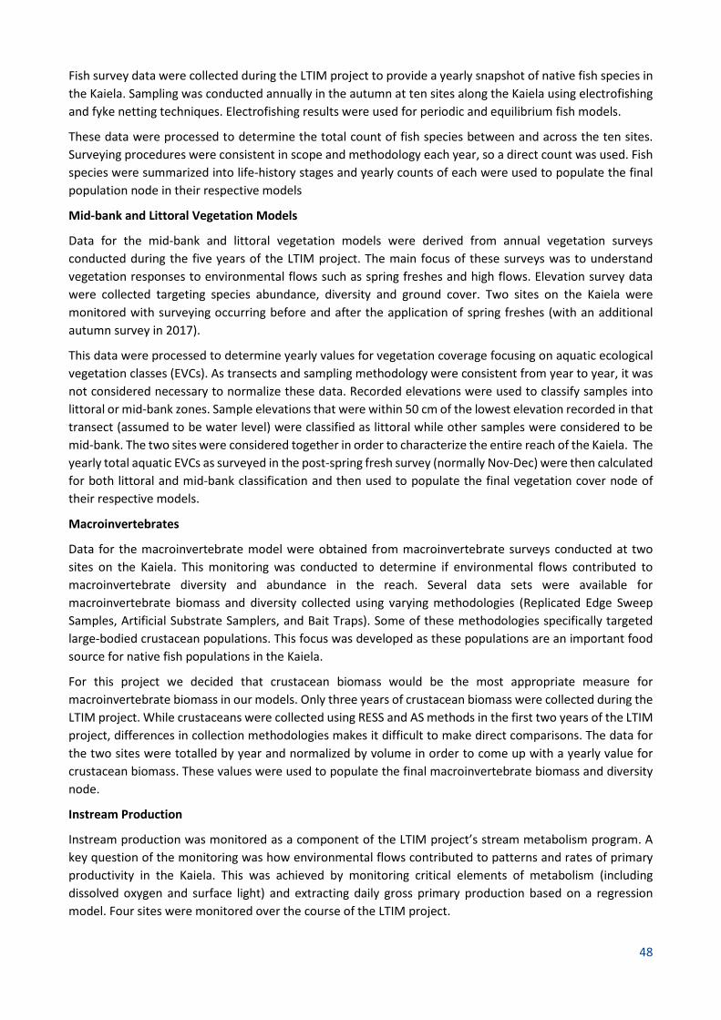
48
Fish survey data were collected during the LTIM project to provide a yearly snapshot of native fish species in the Kaiela. Sampling was conducted annually in the autumn at ten sites along the Kaiela using electrofishing and fyke netting techniques. Electrofishing results were used for periodic and equilibrium fish models.
These data were processed to determine the total count of fish species between and across the ten sites. Surveying procedures were consistent in scope and methodology each year, so a direct count was used. Fish species were summarized into life-history stages and yearly counts of each were used to populate the final population node in their respective models
Mid-bank and Littoral Vegetation Models
Data for the mid-bank and littoral vegetation models were derived from annual vegetation surveys conducted during the five years of the LTIM project. The main focus of these surveys was to understand vegetation responses to environmental flows such as spring freshes and high flows. Elevation survey data were collected targeting species abundance, diversity and ground cover. Two sites on the Kaiela were monitored with surveying occurring before and after the application of spring freshes (with an additional autumn survey in 2017).
This data were processed to determine yearly values for vegetation coverage focusing on aquatic ecological vegetation classes (EVCs). As transects and sampling methodology were consistent from year to year, it was not considered necessary to normalize these data. Recorded elevations were used to classify samples into littoral or mid-bank zones. Sample elevations that were within 50 cm of the lowest elevation recorded in that transect (assumed to be water level) were classified as littoral while other samples were considered to be mid-bank. The two sites were considered together in order to characterize the entire reach of the Kaiela. The yearly total aquatic EVCs as surveyed in the post-spring fresh survey (normally Nov-Dec) were then calculated for both littoral and mid-bank classification and then used to populate the final vegetation cover node of their respective models.
Macroinvertebrates
Data for the macroinvertebrate model were obtained from macroinvertebrate surveys conducted at two sites on the Kaiela. This monitoring was conducted to determine if environmental flows contributed to macroinvertebrate diversity and abundance in the reach. Several data sets were available for macroinvertebrate biomass and diversity collected using varying methodologies (Replicated Edge Sweep Samples, Artificial Substrate Samplers, and Bait Traps). Some of these methodologies specifically targeted large-bodied crustacean populations. This focus was developed as these populations are an important food source for native fish populations in the Kaiela.
For this project we decided that crustacean biomass would be the most appropriate measure for macroinvertebrate biomass in our models. Only three years of crustacean biomass were collected during the LTIM project. While crustaceans were collected using RESS and AS methods in the first two years of the LTIM project, differences in collection methodologies makes it difficult to make direct comparisons. The data for the two sites were totalled by year and normalized by volume in order to come up with a yearly value for crustacean biomass. These values were used to populate the final macroinvertebrate biomass and diversity node.
Instream Production
Instream production was monitored as a component of the LTIM project’s stream metabolism program. A key question of the monitoring was how environmental flows contributed to patterns and rates of primary productivity in the Kaiela. This was achieved by monitoring critical elements of metabolism (including dissolved oxygen and surface light) and extracting daily gross primary production based on a regression model. Four sites were monitored over the course of the LTIM project.

49
For this project we looked at total gross primary production load for the year by totalling up daily loads measured over the course of the year. This was used to populate the final production node in the model.
Bank Stability
Bank condition was monitored over the course of the LTIM project through the use erosion pins deployed at four sites along the Kaiela. Sediment and deposition at these sites was measured on average every three to four months. The aim of this monitoring work was to determine if environmental flows had a negative impact on bank condition and assess how the timing and duration of flows influenced bank structure.
For this project we summarized yearly bank condition by looking at the total amount of erosion at all four sites, as it was necessary to characterize the entire river reach. It was assumed that high levels of erosion indicated lower bank stability, although it is recognized the erosion is a natural process in channel formation. Total erosion for the year was used to populate the final bank stability node.
5.3.2 Outcomes of Data Integration The data were used to update the conditional probability tables (CPTs) that underpin the models. This is done via the expectation maximization algorithm built into Netica, which updates CPT table entries based on data provided, and in consideration of the existing CPT entries. This alters the relationships between drivers and outcomes in the models and thus leads to differences in predictions.
Given that the amount of data is limited to five years for the LTIM project, it is unsurprising that the models were only slightly modified by the data integration process (Table 7). If data integration is expanded to include VEFMAP and CEWO STIM data, we can expect closer to 10-15 years of data for casefiles (depending on the ecological objective) and there is a possibility of more significant modifications to the models. Five years of data, while extensive in the context of ecological datasets, does not fully capture the variability of ecological condition or the range of possible flow scenarios for the river. For the purposes of this project, we have used models without data integration to pair with the flow tool described in this report. We strongly recommend that work continue to incorporate existing data beyond LTIM into the models.
Table 7: Outcomes of data integration. Percentage change to state is the difference in the belief bar percentage of the most common outcome following data integration, when all flow and non-flow driving variables were included in their optimal states. Negative amounts imply that the state became less likely.
Model Data Sets Used Nodes Populated Final Node Measurement
% Change to state
Mid-bank Vegetation Vegetation Survey Mid-bank Vegetation Coverage
Total Aquatic EVCs -2.4
Littoral Vegetation Vegetation Survey Littoral Vegetation Coverage
Total Aquatic EVCs -2.7
Periodic Fish Movement Larvae Survey River Survey
Movement Recruitment Self-Sustaining Fish Population
Sum of fish surveys for life history grouping
-3.5
Equilibrium Fish River Survey Larvae Survey
Self-Sustaining Fish Population Recruitment
Sum of fish surveys for life history grouping
-4.5
Opportunistic Fish River Survey Larvae Survey
Self-Sustaining Fish Population Recruitment
Sum of fish surveys for life history grouping
3.6
Macroinvertebrate Crustacean Bait Traps Macroinvertebrate biomass and diversity
Total biomass 6.2
Bank Stability Bank Condition (Erosion Pins)
Bank Stability Total erosion 1.2
Instream Production Stream Metabolism Instream Production Total instream production for year
1.4
50
5.3.3 Gaps in the data and other shortcomings Data integration into ecological models for the purpose of environmental flows assessment is currently a novel approach and needs further development and refinement. This first data integration attempt has helped us identify several gaps and shortcomings that will need to be overcome for this to become a more widely used method. Integration of data over time will make model predictions more realistic, but we note that this does not necessarily mean that predictions will become more precise (i.e. reduced uncertainty). The stochastic nature of flow-response systems mean that outcomes will always be difficult to predict.
Lack of data for key ecological objectives
There are no data available in the Kaiela system for turtles and platypus. Instream habitat complexity was assessed as part of early environmental flows monitoring (Chee et al. 2009), but these data are well outside the scope of the current project. There are some data for platypus in nearby catchments, but they are not suitable for the purposes of these models. Instream habitat complexity is extremely difficult to measure or monitor, but methodologies could potentially be developed. As instream habitat complexity is a crucial component of the other ecological models, this should be explored in future monitoring projects.
Lack of data for intermediate nodes
All ecological models contain intermediate nodes that are crucial for illustrating and understanding the complex relationships underpinning ecological processes in the Kaiela. However, there are almost no data for these intermediate processes that could be used to populate these nodes. Data from the LTIM project were primarily used to populate the final condition node of the model. The fish models are the most notable exception to this, as larvae and movement data were used to populate key intermediate nodes in the periodic fish model. Directing monitoring of these intermediate processes would help us to better understand the complex flow-ecology relationships and verify/refine model structures.
Suitability of data to final nodes
The final nodes of the models developed for this project were based on the ecological objectives defined in the first workshop. Since the LTIM monitoring data were not explicitly undertaken with these objectives in mind, there needs to be a further discussion around the suitability of these data to the ecological models. For example, the fundamental objective for mid-bank and littoral vegetation is to maximise the structural complexity and diversity of bank vegetation. The LTIM project monitored vegetation by identifying specific species and aquatic EVCs at specified transects. It is difficult to ascertain the structural complexity from these values and total aquatic EVCs was assumed to be a proxy for vegetation condition.
5.3.4 Future Approaches and Monitoring As a first step, the data should be expanded to include data from the VEFMAP and CEWH Short-Term Intervention Monitoring projects, plus other monitoring programs in the Kaiela. Processing these additional data will add at least five more years to some of the case file reports. One issue with this process is the collating of multiple data sets with inconsistent collection methods. Methodologies are sometimes changed over the course of monitoring programs and can be different between monitoring programs that occur in the same areas. This is due to changing priorities in monitoring objectives, fluctuating budgets for projects, and improvements in technologies and measurement methods. This can make it difficult to compare data between years in a rigorous or quantitative way.
Data processing should be refined through further consultation with discipline experts to determine the best ways to measure final conditions and intermediate processes. Additionally, state definitions for the nodes should be further refined based on further monitoring and expert opinion. Nodes within the models have state definitions such as “good-average-poor” or “large-medium-small”, and it can be difficult to define these states for a given population.

51
These models can be improved through continued monitoring extending existing datasets. Additionally, the CMA could undertake targeted monitoring in order to improve model performance and understand ecological responses of specific objectives. Responsive monitoring programs designed with ecological objectives and management priorities in mind are a key component of adaptive management. Outlined in Table 8 are future monitoring recommendations for the Kaiela.
Table 8: Future monitoring recommendations for the Kailea River to support model improvements for environmental flows decisions
Objective Proposed Monitoring Priorities
Turtles Begin monitoring turtle populations through targeted surveys with cathedral and fyke nets during the summer months in key locations on the Kaiela. Exploration of possible citizen science initiatives.
Platypus Begin monitoring platypus populations. Possibility of working as a citizen science program or working in collaboration with other efforts.
Mid-bank and Littoral Vegetation
Monitoring of reproduction of extant vegetation to populate important intermediate nodes and better understand structural relationships
Floodplain Vegetation
Begin monitoring floodplain vegetation coverage and diversity. Recommended to select 1-2 key sites to limit monitoring effort
Equilibrium Fish Expert recommends looking at the influence of flow on Murray cod and trout cod dispersal to populate the connectivity cues and movement node. Nesting condition could be monitored as well to determine flow conditions necessary to support habitat. Survival is one of the driving relationships in the model, so quantification and monitoring for this node would be desirable. One way to explore this would be monitoring of habitat diversity and determining ecohydraulic characteristics of ideal habitat. Exploration of other ways to quantify survival and better understand this structural relationship.
Opportunistic Fish Same as equilibrium
Periodic Fish Recruitment should be adequately monitored. Are fish larvae surveys the most appropriate? Are there more thorough ways to measure and characterize recruitment? As with other fish models, survival should also be addressed through the characterization of the ecohydraulics of habitat condition.
Macroinvertebrates Historically, macroinvertebrate monitoring has focused on measuring diversity as an indicator of river health. The focus in the later years of LTIM of looking at biomass is something that should be continued and extended so that biotic production over years with different flow regimes can be better estimated.
Instream Production
It is strongly recommended that organic matter be monitored on a regular basis including autosamplers for flow events. This would be a significant investment, but organic matter is a key driver of production. It would also be beneficial to increase monitoring of nutrients, but this is also costly. Determining the separate contributions of benthic algae, phytoplankton production, and submerged plant production, with a particular emphasis on benthic algae would be a major advance.
Bank Stability Explore ways of measuring notching and slumping in order to better characterize bank stability. Streamology has been pioneering the use of drone-based photogrammetry to look at wholesale bank changes, mostly in the context of IVT flows (Vietz et al. 2019). As we move towards quantification of the relationships between such events and flow regimes, we will be able to improve probabilistic relationships within the models.
Instream Habitat Complexity
Difficult to monitor or measure this objective, as processes can be large scale and gradual. There may be some possibility to monitor this via aerial imagery using drones, but this would need to be explored further given that the habitat is submerged.

52
6 Flow Scenario testing to inform flow recommendations 6.1 Flow scenario tool The ecological models developed through this project operate as conditional probability networks in the Netica environment. These Netica models can be easily manipulated to see the contribution of flow components (and other inputs) and their effect on ecological outcomes in individual years. However, the Netica interface does not facilitate simple comparisons across multiple models (especially dependent models) and cannot automatically determine the states of the hydrological input nodes, nor can it easily sequence outputs over multiple years.
We have developed an external flow scenario tool to address these shortcomings. This standalone program allows the user to upload flow scenarios as full hydrographs and assess all of the ecological models simultaneously across any number of years. Briefly, the workflow and functionality is described below:
• Users upload a flow scenario specifying unregulated (i.e. tributary) and regulated (i.e. IVT and environmental water) flows for any number of years. Graphical comparison of outcomes is aided by not including more than about 5 years of flow data.
• Users select a directory housing any number of Netica models. The Netica models are automatically interpreted and converted by the flow scenario tool. Changes to the Netica models can be made in Netica, and these will persist when uploaded to the tool.
• The outcomes are calculated for all loaded models across all years in the simulation. Model dependencies, including other model outputs and antecedent conditions are automatically included. These outcomes are shown in a table and graph on the main tool interface. The table sorts the models that are performing well each year and can be configured to focus on good or poor outcomes. Users can toggle the graph to show any specific model outcome or process (node) within a particular model.
• The full numeric and graphical outputs can also be shown. Full simulation results can be saved to an excel spreadsheet, and a window can be opened that shows graphs of the sequence of condition for all models, and a comparison of the starting and ending condition of all models together in one graph.
An example of interface and outputs of the tool is shown in Figure 14. The tool has been made available to the CMA along with resources on how to use it. In addition, we have used the tool to compare several scenarios of environmental water and IVT delivery to gauge performance of the ecological models in predicting outcomes over multiple years. This is further described in section 6.3 below.
It is relevant to note there are some functionalities that are not available in the tool. These include:
• For the assessment of ecological response to future conditions, the user must select their own hypothesised or representative timeseries of unregulated inflow. The tool cannot forecast streamflows.
• The tool cannot predict environmental flow delivery based on flow recommendations. The user must input their own timeseries of environmental water use. Similarly, IVTs must be specified by the user in a way that considers the implied water availability in the timeseries of unregulated flows.
• Non-hydrological inputs (for example, temperature for fish models or fox population for the turtle model) cannot be assessed beyond a user specified default distribution. These must be specified in the Netica model, but will not update year-to-year. The exception to this is dependencies from other models (i.e. bank stability or macroinvertebrate outcomes) which are updated automatically.

53
Figure 14. Example interface and graphical output of the flow scenario tool.
6.2 Flow scenarios We have assessed modelled outcomes across several scenarios to compare whether predicted outcomes across multiple years align with actual observed outcomes and what is expected given known ecological behaviour to certain flow conditions. These scenarios are explained below in Table 9, using a mixture of historic flows and hypothesised regulated flows.
Table 9. Flow scenarios for model testing and evaluation
Flow scenario Description
S1 – historic flows Historic flows at McCoys’ Bridge from 01/01/2004 to 31/03/2020. Includes IVT and environmental water delivery.
S2 – no environmental flows As S1, but with no environmental water delivery.
S3 – optimum environmental flows As S1, but with flow modified to reflect current (i.e. before this project) flow recommendations. This includes some modification of summer flows to be at or below 940 ML/d.
S4 –IVT scenario (high IVTs) As S3, but with IVTs modified to deliver 3000 ML/d from Dec-Apr for 10 out of every 15 years.
Non-hydrological model inputs were set at default uniform distributions when undertaking these flow scenarios. Then, when assessing model outputs, raw outputs were scaled according to the range of possible outcomes considering these default distributions. In other words, model outcomes were adjusted based on the possible outcomes when considering what changes in flow components only can achieve. This allows a better relative comparison of ecological condition and sensitivity to each flow scenario.
6.3 Results The results for each scenario are presented below in Figure 15. Note the flow tool only operates over complete water years (July-June) so 2004 and 2020 are excluded. In addition, 2005 is excluded to remove

54
some sensitivity to assumed antecedent conditions. Antecedent conditions for each model were uniformly set at one third good, average and poor condition (or their equivalent) at the start of the temporal sequence.
Results are presented with a measure of “overall condition” rather than the proportion of good, average and poor. This is calculated using the proportions in each condition, where:
𝑆𝑆𝑆𝑆𝑆𝑆𝑆𝑆𝑆𝑆 =∑ 𝑛𝑛 ∗ 𝑆𝑆𝑐𝑐=𝑔𝑔𝑔𝑔𝑔𝑔𝑔𝑔𝑐𝑐=𝑝𝑝𝑔𝑔𝑔𝑔𝑝𝑝
max (𝑛𝑛), 𝑛𝑛 = �
2, 𝑆𝑆 = 𝑔𝑔𝑆𝑆𝑆𝑆𝑔𝑔1, 𝑆𝑆 = 𝑎𝑎𝑎𝑎𝑔𝑔0, 𝑆𝑆 = 𝑝𝑝𝑆𝑆𝑆𝑆𝑆𝑆
As an example, if a modelled outcome were 100% poor, the overall condition score would be 0. If an outcome were 100% good, the score would be 1. If an outcome were 33% good, 33% average, and 33% poor – the overall score would be 0.5.
There are two reasons for presenting outcomes this way: 1) it allows an easier comparison for the five scenarios in one figure; and 2) it still allows good/average/poor conditions to be distinguished by their weighting on the score calculation. For example, an outcome with 40% poor, 20% average and 40% good would score higher than 40% poor, 40% average and 20% good.

55
2006 2008 2010 2012 2014 2016 2018
Year
0.1
0.2
0.3
0.4
0.5
0.6
0.7R
elat
ive
cond
ition
BankStability
Historic
No eFlow
Opt. eFlowIVT high
2006 2008 2010 2012 2014 2016 2018
Year
0
0.2
0.4
0.6
0.8
1
Rel
ativ
e co
nditi
on
FloodplainVegetation
Historic
No eFlow
Opt. eFlowIVT high
2006 2008 2010 2012 2014 2016 2018
Year
0.4
0.5
0.6
0.7
0.8
0.9
1
Rel
ativ
e co
nditi
on
InstreamProduction
Historic
No eFlow
Opt. eFlowIVT high

56
2006 2008 2010 2012 2014 2016 2018
Year
0.25
0.3
0.35
0.4
0.45
0.5R
elat
ive
cond
ition
LittoralVegetation
Historic
No eFlow
Opt. eFlowIVT high
2006 2008 2010 2012 2014 2016 2018
Year
0.5
0.52
0.54
0.56
0.58
0.6
0.62
Rel
ativ
e co
nditi
on
MacroBiomassDiversity
Historic
No eFlow
Opt. eFlowIVT high
2006 2008 2010 2012 2014 2016 2018
Year
0.32
0.34
0.36
0.38
0.4
0.42
0.44
0.46
Rel
ativ
e co
nditi
on
MidBankVegetation
Historic
No eFlow
Opt. eFlowIVT high
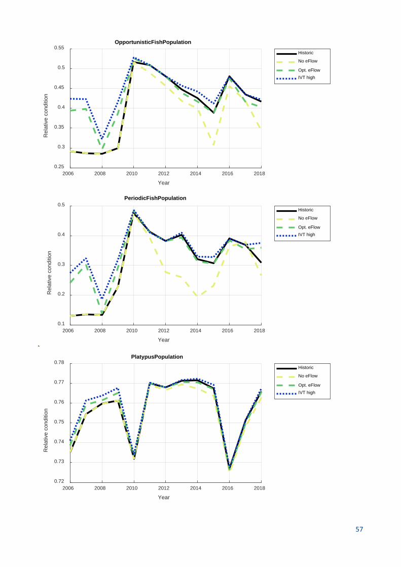
57
2006 2008 2010 2012 2014 2016 2018
Year
0.25
0.3
0.35
0.4
0.45
0.5
0.55R
elat
ive
cond
ition
OpportunisticFishPopulation
Historic
No eFlow
Opt. eFlowIVT high
2006 2008 2010 2012 2014 2016 2018
Year
0.1
0.2
0.3
0.4
0.5
Rel
ativ
e co
nditi
on
PeriodicFishPopulation
Historic
No eFlow
Opt. eFlowIVT high
2006 2008 2010 2012 2014 2016 2018
Year
0.72
0.73
0.74
0.75
0.76
0.77
0.78
Rel
ativ
e co
nditi
on
PlatypusPopulation
Historic
No eFlow
Opt. eFlowIVT high

58
Figure 15. Modelled outcomes for all 12 ecological models across the five flow scenarios.
6.4 Comparison to data
The figure below compares the output for the historical flow scenario with catch data for fish. The modelled outputs align with the catch data well during the latter years of the millennium drought and in the post-drought period when sampled numbers of fish peaked around 2009-11. Equilibrium and opportunistic fish numbers have dropped off more than the model suggested. However the data incorporated here for comparison is electrofishing data only, whereas many opportunistic fish come through fyke nets. We note also that the model suggested a peak in opportunistic fish condition in 2010, which was one of the higher capture years.
2006 2008 2010 2012 2014 2016 2018
Year
0.3
0.32
0.34
0.36
0.38R
elat
ive
cond
ition
TurtlePopulation
Historic
No eFlow
Opt. eFlowIVT high
2006 2008 2010 2012 2014 2016 2018
Year
0.3
0.35
0.4
0.45
0.5
0.55
0.6
Rel
ativ
e co
nditi
on
EquilibriumFishPopulation
Historic
No eFlow
Opt. eFlowIVT high

59
Figure 16. Comparison of historical flow scenario modelled versus fish catch data. The y-axis for capture data has been scaled so that peak modelled condition values coincide approximately with peak fish captures.
0.0
0.2
0.4
0.6
0.8
1.0
0
2
4
6
8
10
12
14
16
18
20
2004 2005 2006 2007 2008 2009 2010 2011 2012 2014 2015 2016 2017 2018 2019 2020
Pred
icte
d re
lativ
e co
nditi
on
Num
ber o
f fis
h pe
r site
±sd
Equilibrium fish
0.0
0.2
0.4
0.6
0.8
1.0
0
2
4
6
8
10
12
2004 2005 2006 2007 2008 2009 2010 2011 2012 2014 2015 2016 2017 2018 2019 2020Pr
edic
ted
rela
tive
cond
ition
Num
ber o
f fis
h pe
r site
±sd
Periodic fish
0.0
0.2
0.4
0.6
0.8
1.0
0
50
100
150
200
250
300
350
400
450
500
2004 2005 2006 2007 2008 2009 2010 2011 2012 2014 2015 2016 2017 2018 2019 2020
Pred
icte
d re
lativ
e co
nditi
on
Num
ber o
f fis
h pe
r site
±sd
Opportunisitic fish

60
A similar comparison was undertaken for bank stability, comparing the predicted relative condition to total erosion at erosion pins (for LTIM monitoring sites). The bank stability model is representative of bank condition along the entire reach, rather than at a point location. There is a discrepancy with the year 2015, but the trend from 2016 to 2018 is matched. The data available on erosion is only a short duration. The outputs from the flow tool suggest that bank stability would have been most impacted in 2010, the year with significant high flow events.
Figure 17. Comparison of historical flow scenario modelled versus bank erosion data.
6.5 Summary In general, modelled outcomes conform to expectations of ecological behaviour under each of the scenarios. Some models were relatively insensitive to scenarios, including floodplain vegetation, instream complexity, platypus and turtles. The most sensitive models were bank stability, littoral and mid-bank vegetation, and all fish models. The insensitivity of platypus and turtle models can be due to their dependence on non-hydrological inputs. Floodplain vegetation is only sensitive to high overbank flows which generally cannot be delivered as environmental water. Hence, floodplain vegetation is insensitive to the five scenarios as they all share common characteristics in overbank flows.
There is a clear trend in the most sensitive models of scenario S2 (historic flows with no environmental water) leading to the poorest ecological outcomes. The are a few exceptions – the bank stability and instream production models show the best outcomes with scenario S2. These two results are not surprising. Banks will be more stable in rivers with less water, as there is less erosive force. For instream production, low flows will greatly increase benthic (stream bed) production because shallower water will attenuate less light. High flow events are also associated with elevated turbidity, which decreases light penetration into the water and therefore production. Littoral vegetation shows some benefits from 2010-2014 under scenario S2. We believe these benefits arise from having relatively stable low flows during this period, which would promote littoral vegetation. Outcomes gradually get worse into 2019, where S2 leads to the lowest overall outcomes.
All fish models generally respond well to the alternate IVT scenario (S4). This is because fish outcomes benefit from higher year-round low flows, with adverse outcomes usually related to low baseflows or poorly timed fresh events. Mid-bank and littoral vegetation models respond poorly to IVT scenarios, likely due to high summer flows affecting survival and reproduction.

61
Across all models, the scenario that led to a trade-off of overall best outcomes was S3 (optimum environmental water). This scenario, whilst not quite delivering the best outcomes for fish, avoids poor outcomes from IVT scenarios for littoral vegetation and bank stability models. It should be noted that there is an apparent disconnect in these scenarios between the outcome for bank stability and the outcome for geomorphic complexity. While bank stability processes are currently considered in the geomorphic complexity model through the summer baseflows node, there is currently no explicit link between the two models. Creating this connection in future iterations of models has been flagged as a topic for future research and could potentially better represent the longer-term impacts of IVTs on bank stability and overall geomorphology.
This demonstration of the flow scenario tool shows that it can be used to make predictions under different hypothesized flow regimes. The tool can be used in annual and multi-annual planning cycles, testing outcomes for different flow regimes, building on the observed antecedent condition for the start year (as opposed to the evenly distributed conditions we used here.

62
7 Determining environmental flow recommendations
7.1 Overview of approach We ran a workshop to use a structured approach to define the environmental flow recommendations. Outputs from the ecological models and flow tool formed significant inputs to this workshop. From the ecological models, developed using robust methods (expert elicitation), the key influencing flow components were identified and presented to the workshop members. The workshop asked participants to firstly prioritise flow components for each individual objective, and then to work in small groups to prioritise flow components across objectives and understand when/and why the priorities might change due to external drivers (such as climate). Refer to Appendix D for a list of workshop documents.
The flow recommendations developed from the workshop were circulated in draft form to project stakeholders for comment and correction. Changes were incorporated into the final recommendations presented below. During this stage, many comments were received relating to the perceived importance of specific flow components for particular ecological outcomes, but for which we did not have evidence in the models that they were important. Flow components were either lacking from models altogether, or the sensitivity analyses had shown that they were less important than indicated in the feedback to the flow recommendations.
The process to work with stakeholders and the technical panel to develop conceptual models and then the quantification of those models with expert opinion was a very structured process. We decided based on this not to include recommendations that were not supported by the discussions around model development and indeed the model outcomes. In this project, we have sought to improve the rigour of ecological predictions to changes in flows. However, such comments may be useful inputs to future revisions of the models and recommendations coming from them. The aim of having these models as the foundation for the flow recommendations is that they can be updated over time with new data and knowledge. We have captured the comments in Appendix F so that they may be considered in future work.
7.2 Environmental Flow Recommendations The final flow recommendations are provided in Table 10. The format of these flow recommendations differs from the traditional approach. The recommendations are given in priority order, where each year the higher priority flow components should be provided where possible before moving down the list. Where there are trade-offs between flow components (e.g. some favour fish over vegetation), these should be considered based on antecedent ecological condition. There is also a column in the table highlighting environmental constraints around delivery. These are recommendations that must be met through river operations, rather than necessarily through the provision of additional environmental water.
Note that the environmental flow recommendations are for McCoy’s bridge near the bottom of the Kaiela. Given that flows are delivered from Goulburn Weir, we don’t see additional value in separate flow recommendations for reach 4 and reach 5. However, if there are significant tributary flows from broken river and seven creeks, releases of environmental water downstream of the weir may be required to ensure targets are met in reach 4. Note also that flow recommendations are delivered at a resolution of no greater than 100 ML/d. We don’t believe that we have sufficiently precise knowledge of either the hydraulics of the river nor the ecological responses to make recommendations at a scale finer than this.

63
Table 10. Environmental Flow Recommendations for the Kaiela.
PRIORITY FLOW COMPONENT
MAGNITUDE DURATION TIMING FREQUENCY ENVIRONMENTAL FLOW CONSTRAINTS or TRADEOFFS
RELEVANT OBJECTIVES and key considerations DISCUSSION
1 Year round Baseflow
(Providing habit diversity and sustaining the
system)
During summer and autumn, preferred flows are between
500 – 1000 ML/d (or unregulated)
During summer and autumn, ensure
variability in flow regime (CV > 0.2)
(e.g. mean of 750 and standard deviation of
150 ML/d)
During winter and spring, ensure flow
greater than 500 ML/d
N/A All year
Every Year Cod season at start of December and importance of lower base flows for the two weeks prior to provide dry banks for anglers
Baseflows > 1000 ML/d at a constant rate for a duration of longer than 7 days may lead to notching and mass failure (slumping)
• Flows with low variability (CV < 0.2) between 1000 ML/d – 2500 ML/d cause the largest notching impacts - critical zone
• Flows above 2500 ML/d also have potential for notching
Higher rate of fall may pose a risk to bank stability through slumping (keep rate of fall <0.15m per day and rise <0.38m per day)
Flows > 1000ML/day for greater than 10 days will lead to damage/loss of littoral vegetation
Flows > 1750 ML/d may cause damage littoral
vegetation
Flows from Sep - Jan that are higher than the flows delivered in late winter challenge platypus by flooding nesting burrows
All Fish – Baseflow for fish passage, at least 40cm and habitat diversity (provided at 500ML/day).
Instream Productivity (to support Macroinvertebrates) - Water depth < 2-3 m for best irradiation of benthic surfaces across substantial part of cross-section. Max of 2000 ML/day above which slack areas are lost (this will decrease viable areas for biofilm growth)
Macroinvertebrates (to support fish, turtles and platypus) – Flows engage with littoral vegetation to provide edge habitat. Ensure higher flows do not destroy instream vegetation
Littoral Vegetation – Regular but small fluctuations will increase the width of the zone of littoral vegetation, improving habitat outcomes for fish and macroinvertebrates.
Midbank Vegetation- Occasional higher summer baseflows provide wetting midbank elevations and maintaining vegetation, however sustained heightened baseflows causing severe inundation would negatively impact vegetation
Bank Stability – Lower, but variable, baseflows are protective against bank notching.
Turtles – No direct effects; affected through benefits of baseflows for macroinvertebrates as a food source
Social – flows greater than 1000 ML/d inundate high-level sand bars and limit access for camping and fishing (particularly important during holidays and through to Jan 25, with consideration during the Easter holidays)
Lower limit in place to ensure depth for fish and platypus passage (500 ML/d provides a depth of 30 – 40 cm).
Upper limit to protect bank stability (slumping and notching), bank vegetation and social needs
While habitat diversity is primarily determined by channel complexity, variable flows will improve habitat diversity by engaging different parts of the channel at different discharges, including slack water and slow velocity and deep pools.
(Refer to hydraulic cross sections showing 500 and 1000 ML/d)
High summer flows identified as an issue for platypus burrows may become more likely under climate change scenarios, with decreased probabilities of high winter flow events being delivered.
Note that the or natural clause here is to allow flows to exceed 1000 ML/d if there is a natural event outside the control of operations.
2a Overbank or high flows
(channel forming event)
Opportunistic event – aim to provide as
high as possible an event by utilising or re-creating natural
events. Where overbank not
possible, still provide as large an event as possible for channel
maintenance and forming.
>30,000 ML/d allow significant area of
floodplain vegetation to be inundated
>20,000 ML/d inundates floodplain
near Loch Garry
Areas on the lower
floodplain will fill
instantaneously.
5 days at peak to fill larger
wetlands (base this on
opportunity to piggyback).
Ideally late winter to spring or as naturally induced
Not during summer to minimize black water events.
As often as possible given natural flow
events.
Aim for an event >10,500 or as high as possible each year (rainfall runoff or release)
>20,000 7 in 10 years or as per natural rainfall
runoff
>30,000
Natural frequency.
Higher rate of fall may pose a risk to bank stability through slumping (keep rate of fall
<20% change per day)
Flows greater than 40,000 ML/d begin to inundate private properties with adverse
social outcomes
Late spring and summer high flows exceeding the high winter flows can have an adverse
impact on platypus juveniles, increasing risks of flooding burrows. Important to monitor
spring flows in relation to winter flows
Late spring flows greater than 22,000 ML/D will have an impact on turtle nesting and
juveniles
Opportunistic Fish – Provides connectivity to off-channel habitats with greater food resources
Periodic/Equilibrium Fish – Provides cues for movement through the system allowing dispersal
Instream Productivity – Return flows bring organic matter from the floodplain and off-channel habitats into the river channel, driving production and respiration
Macroinvertebrates – Benefit from higher instream productivity as a food source
Littoral/Bank Vegetation – Return flows bring large amounts of sediments and propagules into the river channel system rebuilding vegetation habitat
Floodplain Vegetation – Semi-regular inundation of floodplain vegetation is necessary for plant condition and as part of reproductive cycle
There are currently operational constraints that limit the ability to deliver overbank flows and the achievement of this recommendation.
There is also a delivery constraint of 9,500 ML/d release from Lake Eildon. Delivering this event is therefore opportunistic based on high tributary flows and is only likely to be possible in wetter years (requiring GMW not to divert tributary inflows to Waranga Basin). These tributary inflows also play an important role in transporting sediment/propagules.
Note that climate change will alter the frequency of these natural events. This is an area that requires further investigation to consider how to sustain the objectives that require these overbank / high flow events and look at possible alternatives for managing the floodplain. It is important to note that these events are distinct from activities undertaken by the GBCMA to water individual wetlands through the irrigation system. These decisions are made separately with the wetlands environmental water advisory group.
As noted, these are opportunistic flow events. These flows would be generated naturally in the upper and mid Goulburn River and flow past the
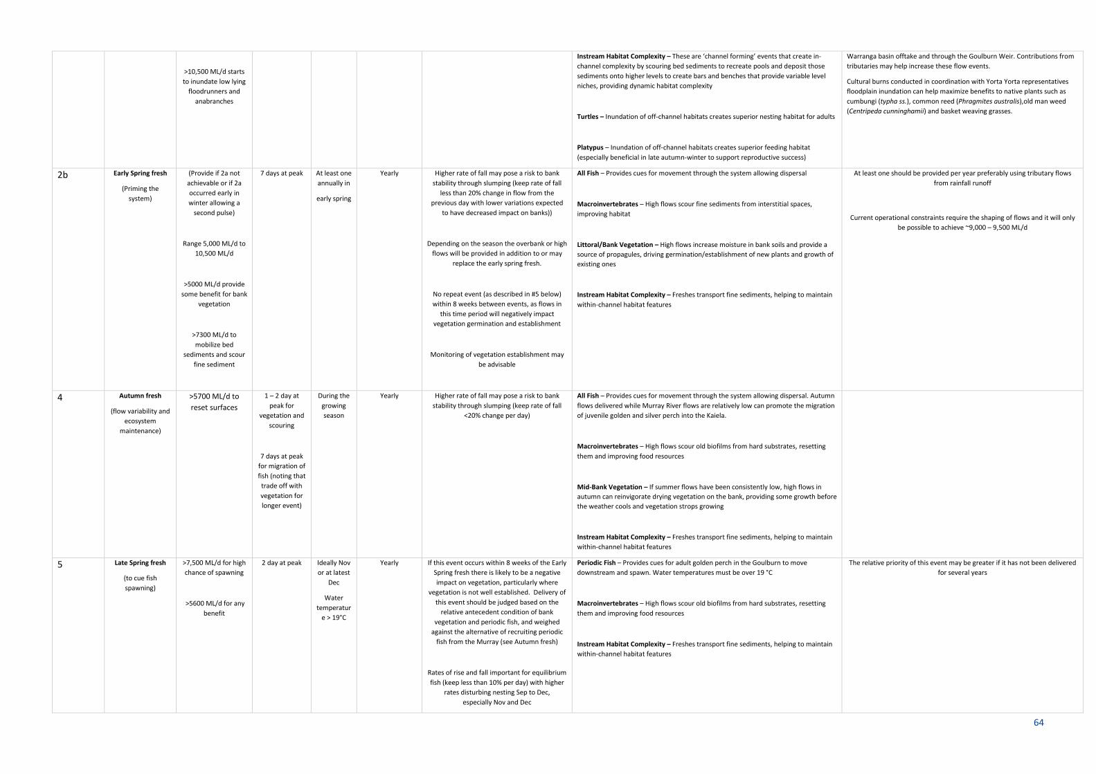
64
>10,500 ML/d starts to inundate low lying
floodrunners and anabranches
Instream Habitat Complexity – These are ‘channel forming’ events that create in-channel complexity by scouring bed sediments to recreate pools and deposit those sediments onto higher levels to create bars and benches that provide variable level niches, providing dynamic habitat complexity
Turtles – Inundation of off-channel habitats creates superior nesting habitat for adults
Platypus – Inundation of off-channel habitats creates superior feeding habitat (especially beneficial in late autumn-winter to support reproductive success)
Warranga basin offtake and through the Goulburn Weir. Contributions from tributaries may help increase these flow events.
Cultural burns conducted in coordination with Yorta Yorta representatives floodplain inundation can help maximize benefits to native plants such as cumbungi (typha ss.), common reed (Phragmites australis),old man weed (Centripeda cunninghamii) and basket weaving grasses.
2b Early Spring fresh
(Priming the system)
(Provide if 2a not achievable or if 2a occurred early in winter allowing a
second pulse)
Range 5,000 ML/d to 10,500 ML/d
>5000 ML/d provide some benefit for bank
vegetation
>7300 ML/d to mobilize bed
sediments and scour fine sediment
7 days at peak At least one annually in
early spring
Yearly Higher rate of fall may pose a risk to bank stability through slumping (keep rate of fall
less than 20% change in flow from the previous day with lower variations expected
to have decreased impact on banks))
Depending on the season the overbank or high flows will be provided in addition to or may
replace the early spring fresh.
No repeat event (as described in #5 below) within 8 weeks between events, as flows in
this time period will negatively impact vegetation germination and establishment
Monitoring of vegetation establishment may be advisable
All Fish – Provides cues for movement through the system allowing dispersal
Macroinvertebrates – High flows scour fine sediments from interstitial spaces, improving habitat
Littoral/Bank Vegetation – High flows increase moisture in bank soils and provide a source of propagules, driving germination/establishment of new plants and growth of existing ones
Instream Habitat Complexity – Freshes transport fine sediments, helping to maintain within-channel habitat features
At least one should be provided per year preferably using tributary flows from rainfall runoff
Current operational constraints require the shaping of flows and it will only be possible to achieve ~9,000 – 9,500 ML/d
4 Autumn fresh
(flow variability and ecosystem
maintenance)
>5700 ML/d to reset surfaces
1 – 2 day at peak for
vegetation and scouring
7 days at peak for migration of fish (noting that trade off with vegetation for longer event)
During the growing season
Yearly Higher rate of fall may pose a risk to bank stability through slumping (keep rate of fall
<20% change per day)
All Fish – Provides cues for movement through the system allowing dispersal. Autumn flows delivered while Murray River flows are relatively low can promote the migration of juvenile golden and silver perch into the Kaiela.
Macroinvertebrates – High flows scour old biofilms from hard substrates, resetting them and improving food resources
Mid-Bank Vegetation – If summer flows have been consistently low, high flows in autumn can reinvigorate drying vegetation on the bank, providing some growth before the weather cools and vegetation strops growing
Instream Habitat Complexity – Freshes transport fine sediments, helping to maintain within-channel habitat features
5 Late Spring fresh
(to cue fish spawning)
>7,500 ML/d for high chance of spawning
>5600 ML/d for any benefit
2 day at peak Ideally Nov or at latest
Dec
Water temperatur
e > 19°C
Yearly If this event occurs within 8 weeks of the Early Spring fresh there is likely to be a negative impact on vegetation, particularly where
vegetation is not well established. Delivery of this event should be judged based on the
relative antecedent condition of bank vegetation and periodic fish, and weighed
against the alternative of recruiting periodic fish from the Murray (see Autumn fresh)
Rates of rise and fall important for equilibrium fish (keep less than 10% per day) with higher
rates disturbing nesting Sep to Dec, especially Nov and Dec
Periodic Fish – Provides cues for adult golden perch in the Goulburn to move downstream and spawn. Water temperatures must be over 19 °C
Macroinvertebrates – High flows scour old biofilms from hard substrates, resetting them and improving food resources
Instream Habitat Complexity – Freshes transport fine sediments, helping to maintain within-channel habitat features
The relative priority of this event may be greater if it has not been delivered for several years

65
Cod season at start of December and importance of lower base flows for the two
weeks prior to provide dry banks for anglers. Noted previously in winter baseflows but a late Spring fresh could also impact opening
6 Winter-Spring variable baseflow
(Ensure habitat diversity)
>500 ML/d - natural
Variability required – mimic natural
variability by passing freshes and larger
events from tributaries
Winter and spring
Every Year Water availability and seasonal conditions may play a role here. Carryover of sufficient
water to ensure that water is available to capitalise on rainfall runoff events in early
season for flow variability.
Water for spring fresh is higher priority.
All Fish – Baseflow for fish passage, at least 40cm and habitat diversity
Macroinvertebrates – Flows engage with littoral vegetation to provide edge habitat.
Littoral Vegetation – Regular fluctuations will increase the width of the zone of littoral vegetation, improving habitat outcomes for fish and macroinvertebrates. However, littoral vegetation is dormant in winter.
Midbank Vegetation- Higher winter baseflows appropriate to season support wetting of midbank soils and vegetation maintenance
Instream Habitat Complexity – Movement of sediment through the system and maintenance of deep pools by passing natural flow events and through the incorporation of tributary inflows
Using a bottom-up method to determine flow requirements the minimum recommendation has therefore been set at 500 ML/d for habitat provision.
However, we know from the natural regime, that winter flows would be significantly higher than summer baseflows. The role these flows play may
well be a knowledge gap, especially given monitoring tends to focus on other seasons. The passing of tributary flows ensures that winter flows do have some variability and larger magnitudes. This recommendation will need
further data and investigation to support.
It is anticipated that the 2a overbank/high bank full event and passing of tributary flows will provide the required variability in average and wet years.
In dry years with little rainfall runoff variability will be much less.

66
A consistent outcome through the process of stakeholder workshops, expert elicitation and setting of flow recommendations was a stakeholder driven desire to see environmental water inundating the lower Kaiela floodplain. Floodplain inundation is expected to have major benefits for floodplain vegetation, instream primary and secondary productivity, with flow-on effects on fish assemblages.
Infrastructure capacity at Lake Eildon, and inundation constraints in the mid-Goulburn mean that it is not possible to deliberately release enough environmental water to achieve bankfull or overbank flows in the lower reaches of the river. Such events would therefore need to be ‘piggy-backed’ on natural inflows into the mid-Goulburn from unregulated tributaries including the Yea and Acheron Rivers, and through similar inflows below Goulburn Weir from Seven Creeks and the Broken River. Constraints also exist in the lower Kaiela, with discharges above ~ 40,000 ML/day inundating private properties on the lower floodplain. Also it is Victorian government policy not to intentionally flood private land without permission. There is no such permission currently for the Goulburn River, so GMW is restricted to current operational limits of 9500ML/day.
Considerable work has been done in the last 10 years examining ways of reducing such constraints and returning water to the lower Kaiela floodplain, but the issues remain unresolved. However, given stakeholder enthusiasm for floodplain inundation, and the modelled scientific benefits, we recommend renewed effort on resolving these constraints, and in the interim, maximizing effort to deliver high winter flows that begin to inundate floodplains (> 20,000 ML/day) or at least inundate low lying flood-runners and anabranch channels (> 10,500 ML/day). Even this lower figure is considerably larger than any environmental flow event previously delivered in the lower Kaiela. Any efforts to allow floodplain inundation should consider the implications of climate change (see discussion in section 8).
An issue of increasing importance in the last 5 years has been the delivery of large amounts of trade water down the channel of the Kaiela as Inter-Valley Transfers. These transfers occur mostly over the summer and autumn months and have been demonstrated to cause damage to both channel structure and vegetation, with recent modelling results also suggesting they are causing declines in native fish populations (Vietz et al. 2019; ARI unpubl. data). Our recommendations reflect that prolonged high flows over summer are expected to cause damage, but they do not specifically address the issue of how best to deliver IVTs through the Kaiela. Beyond IVTs, a similar issue exists for the delivery of environmental water through the Kaiela, but targeted for delivery to the lower Murray River. In these cases, the issue is how to deliver water while either improving ecological outcomes or have a neutral environmental impact.
7.3 Linking the flow recommendations to the ecological model and flow tool The flow tool provides an opportunity to test the flow recommendations and ensure their implementation leads to positive ecological outcomes through the models. It also allows us to determine how long it will take models to respond to a fixed set of flow conditions.
Some of the models will not display equilibrium behaviour, or rather, they will always reach a steady state output after a single year. This is due to two models – instream production and bank stability – not featuring an antecedent condition node in their structure. Without sensitivity to antecedent conditions, the models will simply respond to a given set of conditions immediately in that year. However, all other models will take time to adjust their condition to a fixed set of inputs.
To this end, a timeseries of flows that achieves the full flow recommendations was developed and run through the flow tool to confirm two things:
• The maximum achievable ecological condition predicted by the models through delivering the flow recommendations
• The time taken for each model to achieve this ‘equilibrium’ maximum condition if all other inputs remain the same

67
The timeseries of flow recommendations represents an artificial hydrograph that was developed without considering the natural flow regime of the Kaiela (see Figure 18). Note that Figure 18 includes the recommended rates of rise and fall for each flow component and the magnitude and durations are the maximum recommended. It is simply used to assess how models respond when the full set of flow recommendations is delivered. It should be noted, however, that the full set of recommendations is unlikely to be included in a single year because of simple scheduling issues. Having both early and late spring freshes in this sequence, on the back of the overbank flow event means that the recommended 8-week period between spring freshes for vegetation recovery is not met. Because it was uncertain how long models would take to reach equilibrium, the flow recommendations timeseries was repeated for 10 years through the flow tool.
Figure 18. Example annual timeseries achieving the flow recommendations and average flow in the Kaiela for two time periods.
The antecedent condition for all models was set to 0 (i.e. 100% poor or equivalent) at the start of the simulation. All non-hydrological inputs such as temperature or logging were set to their value that gives the maximum benefit in the models, as the point of the analysis is to see how quickly models can respond to flows.
The output for all models in their overall condition is shown in Figure 19. Some models respond more quickly than others, but the typical range for the equilibrium time is between two and five years. The within-channel vegetation models (littoral and midbank) have a generally low equilibrium condition. This is partly due to their dependence on bank stability, which also has a low equilibrium condition. However, it is important to note that this bank stability condition is very close to the maximum achievable given any combination of inputs (refer to previous sections on ecological models). Littoral and mid-bank vegetation may also be responding negatively to the shorter than recommended time between spring fresh events in this synthetic hydrograph. There appears to be some extra dynamic behaviour occurring in the periodic fish model evident from some ‘bouncing’ in its condition around the steady state value (see Figure 19). This is an interesting result given it has a very similar structure to the opportunistic fish model (which does not display this behaviour), although this is unlikely to have any consequences for future modelling or management.
Jan Feb Mar Apr May Jun Jul Aug Sep Oct Nov Dec Jan
Date 2001
0
0.5
1
1.5
2
2.5
3
Dai
ly fl
ow (M
L/d)
10 4
Flow recommendations
Avg. 1977-2011
Avg. 2012-2019
Summer/autumn baseflow
Autumn fresh
Overbank flow Early spring fresh
Late spring fresh
Winter/spring baseflow

68
The equilibrium time is taken to be the time when models reach 95% of their steady state condition. Table 11 shows the equilibrium time and steady state value for all models.
Table 11. Equilibrium overall condition and time taken to reach this for each model when the flow recommendations are delivered.
Models Equilibrium overall condition from flow recommendations
Equilibrium time (years)
Bank Stability 0.42 n/a
Floodplain Vegetation 0.64 1
Geomorphic Complexity 0.87 5
Instream Production 0.64 n/a
Littoral Vegetation 0.35 4
Macro Biomass Diversity 0.61 2
MidBank Vegetation 0.38 4
Opportunistic Fish Population 0.55 3
Periodic Fish Population 0.41 3
Platypus Population 0.88 3
Turtle Population 0.72 3
Equilibrium Fish Population 0.48 3
None of the models reach a steady state condition of 100% even following repeated delivery of all environmental flow components. There are several reasons for this.
• The results in Figure 19 are the proportion of maximum possible condition achievable through flow manipulation. The results show that it is not possible to simultaneously maximize benefit for all ecological endpoints in the river, even with unlimited environmental water.
• The overall condition index is a composite of the different states of potential outcome (e.g. Good, Average, Poor). It is not a deterministic prediction of condition.
• We have deliberately forced experts to state their uncertainties in the parameterization of the ecological response models. It is not realistic to be 100% confident of an ecological outcome regardless of how much environmental water is used. Unforeseen events and poorly understood processes mean that ecological outcomes will always be predicted with uncertainty. This is also incorporated into the calculation of the overall condition index.

69
Figure 19. Model responses to achieving a repeating series of the flow recommendations.
7.4 Potential implications of climate change Our ability to deliver environmental flow recommendations such as those outlined above will be affected by future climate. There are significant uncertainties in both how the climate will change and how realised changes will affect the delivery of environmental water and associated ecological outcomes. Nonetheless, changes in climate will affect unregulated hydrologic regimes and the movement of regulated water in the Kaiela through changes to water allocation and demands. We have investigated some plausible scenarios of how climate change may affect flows at McCoy’s Bridge through a combination of rainfall-runoff and river operations modelling.
One possible method would be to compare historical timeseries (for “current”) with those derived from Global Climate Models (GCMs) (for “future”), which is what was done in Section 6.2. However, this is somewhat limiting, for two reasons: (i) future sequences could unfold in many different ways and are unlikely to repeat past sequences, even if future climate were not changing; and (ii) since GCMs are simplifications of the climate system, their outputs are qualitatively different to historic timeseries. These differences could confuse the overall message about the effect of climate change when directly comparing their outputs with historic timeseries. Thus, a method is needed in which the “current” and “future” flows are qualitatively similar, and the only difference is the climatic conditions. For this purpose, we adopt stochastic data generated under the concurrent ARC Linkage Project (LP1701100598, Vulnerabilities for Environmental Water Outcomes in a Changing Climate), which focuses on Kaiela environmental flow management.
0 1 2 3 4 5 6 7 8 9 10
Number of years
0
0.1
0.2
0.3
0.4
0.5
0.6
0.7
0.8
0.9
1O
vera
ll co
nditi
on
Steady state outputs from achieving flow recommendations
BankStability
FloodplainVegetation
GeomorphicComplexity
InstreamProduction
LittoralVegetation
MacroBiomassDiversity
MidBankVegetation
OpportunisticFishPopulation
PeriodicFishPopulation
PlatypusPopulation
TurtlePopulation
EquilibriumFishPopulation
BankStability FloodplainVegetation GeomorphicComplexityInstreamProduction LittoralVegetation MacroBiomassDiversity
MidBankVegetation OpportunisticFishPopulation PeriodicFishPopulation
PlatypusPopulation TurtlePopulation EquilibriumFishPopulation

70
As summarised in Appendix F, the stochastic data are first generated focussing on annual dynamics, which ensures that the synthetic data contains appropriate multi-year dry periods and wet periods. Successive disaggregation steps are then applied, first to monthly timestep (to mimic observed seasonal patterns) and later to daily timestep using the custom-built disaggregation approach developed for the Linkage Project (K. Fowler, unpubl.). In between the two disaggregation steps, the monthly flow is passed through the river operations model developed for the Linkage Project. This model is able to simulate IVT deliveries and environmental water management based on historic practices and current flow recommendations; hence modelled outputs show what is possible with current regulated water management. It is important to note that this model does not explicitly model the Broken River catchment and flow, hence these inflows are derived using statistical methods.
We define three scenarios relating to plausible future climate. The future flows scenarios are based on stochastic data, but the data have been shifted to reflect plausible future changes in climatic conditions (see Table 12). In general, these shifts are consistent with GCM projections for a twenty year planning horizon and a high emissions scenario (RCP 8.5). However, it is noted the various GCMs provide a range of future projections (see e.g. www.climatechangeinaustralia.gov.au).
Table 12. Climate change scenarios applied to stochastic data.
Climate scenario Change in mean annual rainfall
Change in mean temperature Change in rainfall seasonality
Wet + 10% + 1°C None
Moderate - 5% + 1°C None
High impact - 10% + 2°C 3% of wet season rainfall redistributed to dry season
Future flow scenarios are shown in the context of contemporary observed flows at McCoy’s Bridge. Since water management in the Kiaela river is evolving through time (with increasing IVTs and environmental water entitlements) we have chosen to restrict comparison to the period of 2012-2020, which reflects a more relevant contemporary flow regime rather than the significantly different earlier historical conditions. We have also modelled one other scenario without climatic changes but with reduced IVT deliveries reflecting a 50% reduction in mean annual IVT volume and variation. Scenario results are shown in Figure 20. In these figures, each year of stochastic data is shown as a separate climate replicate, with the overall flow regime inferred from the median of individual years. This allows an assessment of how natural climatic variability influences the range of hydrologic conditions. We also show some indicative flow thresholds related to typical flow rates for several flow components, where:
• Overbank flow is 30,000 ML/d, which allows significant areas of floodplain vegetation to be inundated
• High/bankfull flow is 10,500 ML/d, which starts to inundate low-lying flood runners and anabranches and is the maximum recommended spring fresh
• Fresh is 7,500 ML/d, which provides the maximum benefit for sediment scouring and fish spawning
• Low or minimum fresh is 5,600 ML/d, which provides most of the benefits for early and late spring, and autumn freshes
• Typical baseflow is 1,000 ML/d, the maximum recommended baseflow for summer/autumn
• Low baseflow is 500 ML/d, the minimum recommended baseflow for all periods

71
Figure 20. Results of three climate change and one IVT scenario on the flow regime at McCoy's Bridge.
In assessing the outcomes of these scenarios, it is worth emphasising that a detailed exploration of the vulnerability of environmental water objectives to climate change is part of the ongoing Linkage Project. The intent of the results provided here is to provide some initial commentary on how climate change may affect our ability to deliver environmental flow recommendations.
It is clear that a wetter climate future will assist in providing ecologically-relevant flows. However, this may also lead to adverse outcomes related to high flows, particularly relevant for bank vegetation and bank stability. It was noted also that a wetter future can increase the downstream demand for IVTs.
In a moderate climate scenario with 5% reduction in long-term annual rainfall the ability to deliver certain baseflow components can reduce by up to approximately 10% of typical conditions from 2012-2020. In a high impact scenario this reduction is approximately 20%, and puts particular stress on maintaining baseflows. Under both of these scenarios natural very high flow events (<1% exceedance) are significantly reduced, which would significantly impact our ability to deliver water to the lower Kaiela floodplain through piggy-backing natural flow events.
Reductions in IVT volumes may affect year-round baseflows, although these results show they are unlikely to have a large impact on high flows or freshes.

72
7.4.1 Implications of changes to overbank flows During the project, the question of changes in the future frequency of overbank flows has been raised, and we conclude this section by commenting on this issue. First, we wish to stress that it is a specialised and complicated question, and that providing the best possible answer would require a separate study, possibly using different methods to those above.
Nonetheless, certain drivers of change are represented in the modelling method and thus it is possible to estimate changes in frequency of overbank flows, albeit subject to significant limitations. As already mentioned in Section 6.2, future changes in floods will likely be driven by the interplay between rainfall intensities (which are expected to increase for rare events) and soil moisture (which is expected to decrease on average). With the exception of the largest floods, it is expected that the drier soil moisture will win out, leading to less frequent small-to-medium floods. Here, ‘small-to-medium’ means an average recurrence interval less than 20 years, and most overbank floods are in this category.
A significant limitation of the present approach is that it does not take into account climate-induced changes in rainfall intensity. However, it does account for drier soils via a two-pronged approach (see also Appendix F): firstly, lower average rainfall means lower simulated monthly streamflow and drier soil moisture in the adopted monthly rainfall runoff model (WAPABA). Secondly, when disaggregating to daily flows, the method dynamically responds to the lower simulated soil moisture by selecting daily flow patterns from historic periods that had similarly dry soils. Both of these factors will affect the number of simulated overbank events.
Comparing the scenarios, the proportion of years with an overbank event is detailed below in Table 13. The “current” scenario refers to stochastic data with no simulated impacts. Note two thresholds for overbank flooding are investigated: 15,000 ML/d and 30,000 ML/d, and no duration is associated with events. The “current climate” stochastic sequences lead to overbank flooding in 79% and 38% of years for the two thresholds, respectively. Whereas the “moderate climate” stochastic sequences lead to overbank flooding in 67% and 26% of years, a reduction in raw terms of 15% and 32%, suggesting that higher overbank flows may be significantly more affected under climate change. When analysing these numbers, it is important to consider that long dry spells and wet spells typical for Australian climate may lead to extended periods of high or low flows. For example, in the high impact climate scenario, although the average proportion of years with flows over 30,000 ML/d was 12%, there was a sequence of 53 years consecutively below the threshold within the 110 years of simulated data. Although these estimates have significant limitations as outlined above, it is hoped this information is useful for planning purposes and future refinement of flow recommendations and ecological priorities.
Table 13. Changes in overbank flooding from the modelled climate scenarios
Scenario Percentage of years with overbank flows (15,000 ML/d)
Percentage of years with overbank flows (30,000 ML/d)
Current climate 79% 38%
Wet climate 85% 57%
Moderate climate impacts 67% 26%
High climate impacts 43% 12%
7.4.2 Climate change flow scenarios and ecological responses The flow tool can also be used to assess what the different climate scenarios mean for long-term ecological outcomes. By implementing the 110-year stochastic sequences through the flow tool, longer-term responses can be assessed by looking at overall changes in the distribution of modelled ecological condition. In these scenarios, non-flow inputs are kept at a default (uniform) distribution. Some of these non-flow drivers may be correlated with different degrees of climate change, for example, water temperature used in the fish
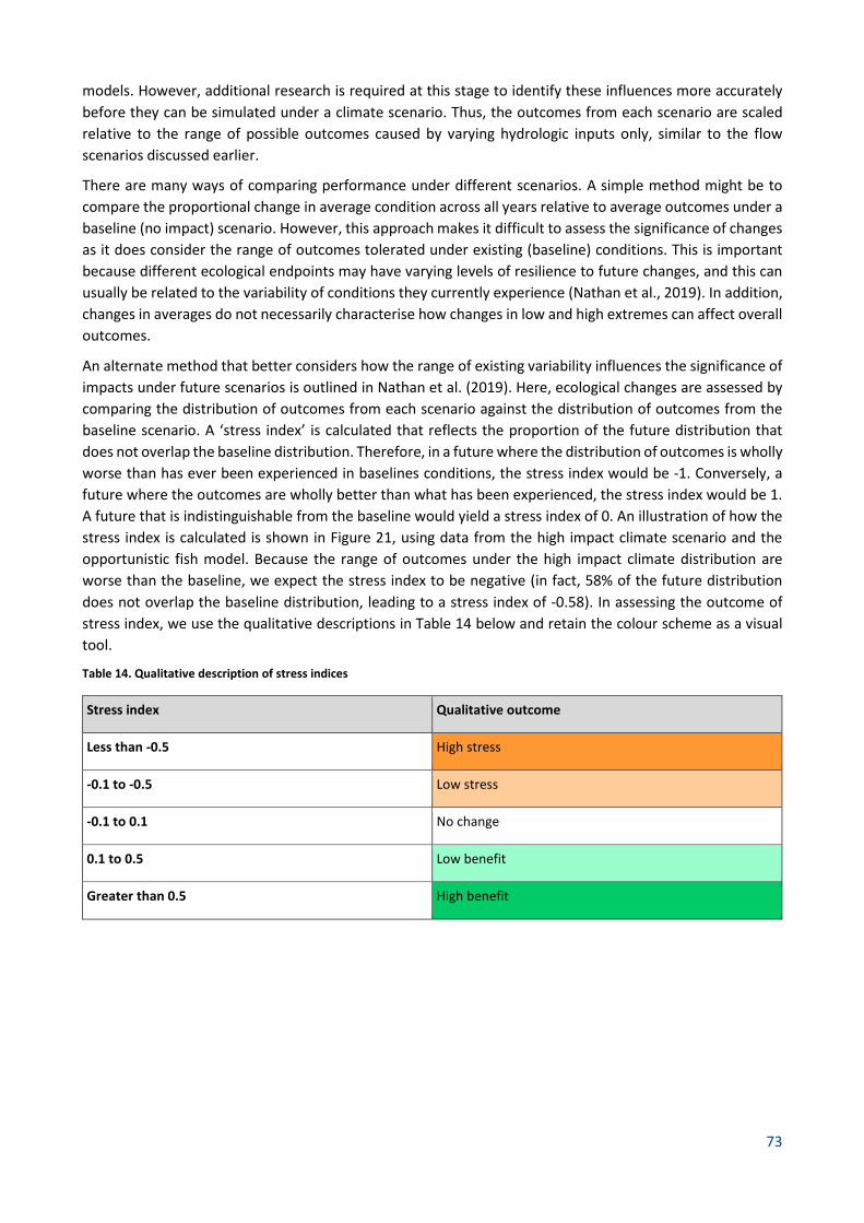
73
models. However, additional research is required at this stage to identify these influences more accurately before they can be simulated under a climate scenario. Thus, the outcomes from each scenario are scaled relative to the range of possible outcomes caused by varying hydrologic inputs only, similar to the flow scenarios discussed earlier.
There are many ways of comparing performance under different scenarios. A simple method might be to compare the proportional change in average condition across all years relative to average outcomes under a baseline (no impact) scenario. However, this approach makes it difficult to assess the significance of changes as it does consider the range of outcomes tolerated under existing (baseline) conditions. This is important because different ecological endpoints may have varying levels of resilience to future changes, and this can usually be related to the variability of conditions they currently experience (Nathan et al., 2019). In addition, changes in averages do not necessarily characterise how changes in low and high extremes can affect overall outcomes.
An alternate method that better considers how the range of existing variability influences the significance of impacts under future scenarios is outlined in Nathan et al. (2019). Here, ecological changes are assessed by comparing the distribution of outcomes from each scenario against the distribution of outcomes from the baseline scenario. A ‘stress index’ is calculated that reflects the proportion of the future distribution that does not overlap the baseline distribution. Therefore, in a future where the distribution of outcomes is wholly worse than has ever been experienced in baselines conditions, the stress index would be -1. Conversely, a future where the outcomes are wholly better than what has been experienced, the stress index would be 1. A future that is indistinguishable from the baseline would yield a stress index of 0. An illustration of how the stress index is calculated is shown in Figure 21, using data from the high impact climate scenario and the opportunistic fish model. Because the range of outcomes under the high impact climate distribution are worse than the baseline, we expect the stress index to be negative (in fact, 58% of the future distribution does not overlap the baseline distribution, leading to a stress index of -0.58). In assessing the outcome of stress index, we use the qualitative descriptions in Table 14 below and retain the colour scheme as a visual tool.
Table 14. Qualitative description of stress indices
Stress index Qualitative outcome
Less than -0.5 High stress
-0.1 to -0.5 Low stress
-0.1 to 0.1 No change
0.1 to 0.5 Low benefit
Greater than 0.5 High benefit

74
Figure 21. Example illustration of the stress index. For opportunistic fish and the high climate impact scenario, 58% of the distribution of outcomes across 110 years lies to the left (i.e. is worse than) the distribution of outcomes under the baseline scenario, leading to a stress index of -0.58.
The overall average ecological condition for each model and each scenario is given in Table 15. The stress index calculated from each scenario distribution relative to the baseline scenario is given in Table 16. The stress indices are consistent with the changes in average outcomes for the scenarios, but give a better indication of the significance of changes. Nonetheless we have included the average outcomes for completeness. The model outputs show some clear winners and losers under the various scenarios. For high climate impacts (the driest scenario), floodplain vegetation, geomorphic complexity, macroinvertebrates, opportunistic and equilibrium fish are all significantly negatively impacted. Conversely, bank stability, littoral vegetation and platypus show significant improvement in their overall condition. This is generally consistent with the earlier flow scenarios – less bank stability problems are expected in a river with less water. The bank stability model feeds into the platypus model which may be responsible for performance improvements, but also there may be fewer spring events affecting burrow habitat quality. Littoral vegetation outcomes are likely improved through high climate impacts leading to lower availability of IVT water.
The moderate climate impacts are in the same direction as the high climate impacts the proportional change in stress index differs for each model. For example, the proportional difference in the stress indices for opportunistic fish are greater than floodplain vegetation, although both are negatively impacted. The wet climate scenario essentially leads to the opposite outcomes compared to the former drier scenarios, although the magnitude of stress indices is lower compared to high climate impacts. Bank stability, mid bank vegetation and instream production condition is reduced, and fish, floodplain vegetation and geomorphic complexity is improved. The wet climate scenario increases both allocations for environmental water use and the potential delivery of IVTs which may interact to dampen stress indices within the in-channel vegetation models sensitive to high summer flows.
In assessing these outputs, it must again be stated that this is an active area of research. Identifying the precise mechanisms responsible for individual model performance to each scenario lies beyond the scope of the current investigation. It is expected that the previously discussed limitations will be reduced as methods
OpportunisticFishPopulation
0.4 0.42 0.44 0.46 0.48 0.5 0.52 0.54 0.56 0.58 0.6
Overall outcome
0
5
10
15
20
25
Freq
uenc
yNo climate impacts
High climate impacts
Proportion of future distribution used to calculate the stress index

75
and models are improved over time, and our understanding of the mechanisms influencing specific ecological responses increases.
Table 15. Overall average outcome across the 110-year simulation for each model and scenario.
Model No impact High climate impacts
Moderate climate impacts
Wet climate
Bank Stability 0.27 0.43 0.35 0.22
Floodplain Vegetation 0.39 0.15 0.26 0.46
Geomorphic Complexity 0.89 0.85 0.87 0.89
Instream Production 0.87 0.95 0.92 0.82
Littoral Vegetation 0.35 0.41 0.36 0.35
Macro Biomass Diversity 0.57 0.55 0.56 0.58
MidBank Vegetation 0.44 0.43 0.44 0.44
Opportunistic Fish Population 0.48 0.43 0.46 0.50
Periodic Fish Population 0.38 0.32 0.35 0.41
Platypus Population 0.73 0.75 0.74 0.72
Turtle Population 0.35 0.35 0.35 0.36
Equilibrium Fish Population 0.52 0.46 0.49 0.54
Table 16. Stress indices calculated for each model and scenario. Colours refer to the qualitative descriptions given in Error! Reference source not found..
Models High climate impacts
Moderate climate impacts
Wet climate
Bank Stability 0.66 0.38 -0.24
Floodplain Vegetation -0.51 -0.45 0.13
Geomorphic Complexity -0.59 -0.35 0.15
Instream Production 0.45 0.24 -0.21
Littoral Vegetation 0.76 0.19 0.04
Macro Biomass Diversity -0.52 -0.34 0.33
Mid Bank Vegetation 0.12 0.16 -0.13
Opportunistic Fish Population -0.58 -0.28 0.34
Periodic Fish Population -0.48 -0.30 0.13
Platypus Population 0.55 0.27 -0.10
Turtle Population -0.20 -0.05 0.11
Equilibrium Fish Population -0.56 -0.35 0.35

76
8 Recommendations for future activities to inform environmental flows in the Kaiela
To conclude this report, we briefly outline four areas that have been identified for further activities to inform environmental flow requirements and management in the Kaiela into the future.
8. Traditional Owner engagement
The Yorta Yorta Nation was engaged through the steering committee of the project during the early stages and attended the first 2 workshops. However staff changes, resourcing and COVID-19 reduced engagement in the later stages of the project.
There is real potential to enhance environmental water management through engagement with the Yorta Yorta Nation, where possible looking for mutual outcomes by making links to cultural flows and integrating their knowledge and understanding of country. The CMA is working to build links with the Yorta Yorta Nation around environmental water management. The currently Commonwealth-funded Monitoring, Evaluation and Research Program is seeking to better engage with the Yorta Yorta Nation, with a view to indigenous knowledge informing the next round of monitoring design. This could provide impetus to improve engagement in the management of environmental water as well.
9. Model reviews and link to monitoring and data collection
The ecological models that have been developed in this project are specifically aimed at supported environmental water management decisions. In their current form, they are predominantly populated by expert opinion. To remain relevant, it is important that these models are updated overtime with new knowledge. One way to do this is to link the models to monitoring and data collection and gradually refine the models to become more data dependent. A formal review point could be nominated at which the model structures could be examined to see if they still capture latest knowledge regarding environmental processes. Such a review would be a significant undertaking because, unless data sets were sufficient to populate the models unaided, expert elicitation would need to be re-done for substantial proportions of the models.
10. Further investigation of options to deliver flows onto the floodplain
The flow recommendations highlight the importance of overbank and bankfull events; all stakeholders agreed on this. A number of the previously explored approaches to putting water on to the floodplain would require significant investment in infrastructure. Further investigations into the implications of climate change that specifically address impacts on high flow events should be undertaken prior to inform decisions around how best to reengage the floodplain.
11. Targeted monitoring and investigations to better understanding of role of winter and spring flows
Winter and spring base flows appear low in the priority list and play only small roles in the ecological models. The natural flow paradigm, along with research and monitoring from other system, demonstrates the ecological importance in having relatively larger seasonal baseflows in the winter and spring months, as these would have occurred under natural conditions. However, using a designer approach and driving the flow recommendations through direct links to ecological outcomes, the role of these flows is less clear. This may well be a result of previous monitoring efforts focussing on the role of summer flows and freshes. We

77
recommend specific consideration of the role of winter and spring baseflows and the implications for each of the objectives.
12. Role of bank stability in overall geomorphic complexity
The flows scenario tool output highlighted an apparent incongruity between the bank stability model and the geomorphic complexity model. Put simply, IVT flows had clear negative impacts on bank stability but little apparent impact on geomorphic complexity. Processes similar to those in the bank stability model appear in the geomorphic complexity model as contributors to the ‘regular channel formation’ node. The sensitivity analysis showed this node to be five times less influential on overall geomorphic complexity than the larger, but much rarer, events that drive ‘wholesale channel formation’. Further research, monitoring and expert elicitation should be used to assess whether the balance of processes in the geomorphic complexity model is appropriate. The current focus on IVT flows and attendant bank stability issues could be resulting in an ‘availability bias’ whereby participants rate a familiar process as being more important simply because they are thinking about it more. Alternatively, it could be that the different way in which bank stability was incorporated into the geomorphic complexity model has reduced the actual importance of this process in predictions of geomorphic complexity. Given that IVTs are likely to continue to be an important part of the water management landscape in the Kaiela, resolving these uncertainties is of high priority
13. Exploration of role of Goulburn Environmental Flows and Goulburn system to delivery of Murray River environmental and consumptive objectives (IVTs)
Although the flow recommendations reported here have greater consideration of the effects of unseasonal summer flows, they do not attempt to answer the specific question of how to deliver consumptive and environmental water to the Murray River through the Kaiela. Several of the comments in Appendix E touched upon this aspect of flow management. As noted in this report, the operational environment, particularly for IVTs is rapidly changing. Longer lead times on IVT and environmental flow orders for the lower Murray system may allow for improved deliveries in the Kaiela. These opportunities should be explored such that flow management may be optimized to allow for simultaneous consumptive and environmental outcomes.
14. Consideration of the role of the Goulburn River within the Basin
The flow objectives identified for the Kaila River are based on the values and outcomes identified by local community and the CMA. There is also a role for the Goulburn River in contributing to downstream values and health of the Basin. This link has not been explored through this flow study.

78
9 References ACREMAN, M., ARTHINGTON, A. H., COLLOFF, M. J., COUCH, C., CROSSMAN, N. D., DYER, F., OVERTON, I., POLLINO, C.
A., STEWARDSON, M. J. & YOUNG, W. 2014. Environmental flows for natural, hybrid, and novel riverine ecosystems in a changing world. Frontiers in Ecology and the Environment, 12, 466-473.
ARTHINGTON, A. 2012. Environmental Flows: Saving Rivers in the Third Millennium, University of California Press. BUNN, E. S. & ARTHINGTON, A. 2002. Basic Principles and Ecological Consequences of Altered Flow Regimes for
Aquatic Biodiversity. Environmental Management, 30, 492-507. CHEE, Y., WEBB, A., STEWARDSON, M. & COTTINGHAM, P. 2009. Victorian Environmental Flows Monitoring and
Assessment Program: Monitoring and assessing environmental flow releases in the Goulburn River. Melbourne: eWater Cooperative Research Centre.
COTTINGHAM, P., KOSTER, W., ROBERTS, J. & VIETZ, G. 2018. Assessment of potential inter-valley transfers (IVT) of water from the Goulburn River.: Report prepared for the Goulburn Broken Catchment Management Authority. .
COTTINGHAM, P. & SKM 2011. Environmental water delivery: lower Goulburn River. Report prepared for Commonwealth Environmental Water, Department of Sustainability, Environment, Water, Populations and Communities. Canberra.
DE LITTLE, S. C., CASAS-MULET, R., PATULNY, L., WAND, J., MILLER, K. A., FIDDLER, F., STEWARDSON, M. J. & WEBB, J. A. 2018. Minimising biases in expert elicitations to inform environmental management: case studies from environmental flows in Australia. Environmental Modelling & Software, 100, 146-158.
DELWP (2016). Goulburn Constraints Measure Business Case – Phase 2 Investigations. Department of Environment, Land, Water and Planning, East Melbourne, Victoria.
DELWP 2017. VEFMAP Stage 6 Part B: Program design and monitoring methods. A report by Arthur Rylah Institute for Environmental Research and Integrated Water and Catchments Division. Melbourne: Department of Environment, Land, Water and Planning.
DEPARTMENT OF ENVIRONMENT LAND WATER AND PLANNING (VIC) 2016. Water For Victoria: Water Plan. Melbourne: State Government Victoria.
FREUND, M., HENLEY, B. J., KAROLY, D. J., ALLEN, K. J. & BAKER, P. J. 2017. Multi-century cool- and warm-season rainfall reconstructions for Australia's major climatic regions. Clim. Past, 13, 1751-1770.
GAWNE, B., BROOKS, S., BUTCHER, R., COTTINGHAM, P., EVERINGHAM, P. & HALE, J. 2013. Long Term Intervention Monitoring Project Monitoring and Evaluation Requirements Goulburn River for Commonwealth environmental water. Final Report prepared for the Commonwealth Environmental Water Office by the Murray-Darling Freshwater Research Centre.
GAWNE, B., HALE, J., STEWARDSON, M. J., WEBB, J. A., RYDER, D. S., BROOKS, S. S., CAMPBELL, C. J., CAPON, S. J., EVERINGHAM, P., GRACE, M. R., GUARINO, F. & STOFFELS, R. J. 2020. Monitoring of environmental flow outcomes in a large river basin: The Commonwealth Environmental Water Holder's long‐term intervention in the Murray–Darling Basin, Australia. River Research and Applications, 36, 630-644.
GBCMA 2014. Goulburn Broken Waterway Strategy 2014-2022. Shepparton: Goulburn Broken Catchment Management Authority.
GBCMA 2017. Goulburn River January 2017 blackwater event. Event summary and GBCMA actions. Shepparton: Goulburn Broken Catchment Management Authority.
GBCMA 2018. Goulburn River seasonal watering proposal 2018/2019. Shepparton: Goulburn Broken Catchment Management Authority.
HANEA, A., MCBRIDE, M., BURGMAN, M., WINTLE, B., FIDLER, F., FLANDER, L., TWARDY, C., MANNING, B. & MASCARO, S. 2017. I nvestigate D iscuss E stimate A ggregate for structured expert judgement. International Journal of Forecasting, 33, 267-279.
HIRABAYASHI, Y., MAHENDRAN, R., KOIRALA, S., KONOSHIMA, L., YAMAZAKI, D., WATANABE, S., KIM, H. & KANAE, S. 2013. Global flood risk under climate change. Nature Climate Change, 3, 816-821.
HORNE, A. C., NATHAN, R., POFF, N. L., BOND, N. R., WEBB, J. A., WANG, J. & JOHN, A. 2019. Modeling Flow-Ecology Responses in the Anthropocene: Challenges for Sustainable Riverine Management. BioScience, 69, 789-799.
HUMPHRIES, P., COOK, R. A., RICHARDSON, A. J. & SERAFINI, L. G. 2006. Creating a disturbance: Manipulating slackwaters in a lowland river. River Research and Applications, 22, 525-542.
KOSTER, W., CROOK, D. A., DAWSON, D. & MOLONEY, P. 2012. Status of fish populations in the lower Goulburn River (2003-2012). Heidelberg, Victoria: Arthur Rylah Institute for Environmental Research, Department of Sustainability and Environment.
MOONEY, W. & CULLEN, A. 2019. Implementing the Aboriginal Waterways Assessment tool: collaborations to engage and empower First Nations in waterway management. Australasian Journal of Environmental Management, 26, 197-215.

79
NIELSEN, D. L., COOK, R. A., NING, N., GAWNE, B. & PETRIE, R. 2016. Carbon and nutrient subsidies to a lowland river following floodplain inundation. Marine and Freshwater Research, 67, 1302-1312.
POFF, L., ARTHINGTON, A. & THARME, R. 2017. Evolution of environmental flows assessment science, principles and methodologies. In: HORNE, A., WEBB, J. A., STEWARDSON, M., RICHTER, B. & ACREMAN, M. (eds.) Water for the Environment: From Policy and Science to Implementation and Management. 1 ed. Cambridge, MA: Academic Press.
POFF, N. L. 2018. Beyond the natural flow regime? Broadening the hydro-ecological foundation to meet environmental flows challenges in a non-stationary world. Freshwater Biology, 63, 1011-1021.
POFF, N. L., ALLAN, J. D., BAIN, M. B., KARR, J. R., PRESTEGAARD, K. L., RICHTER, B. D., SPARKS, R. E. & STROMBERG, J. C. 1997. The Natural Flow Regime - A paradigm for river conservation and restoration. BioScience, 47, 769 - 784.
POFF, N. L. & MATTHEWS, J. H. 2013. Environmental flows in the Anthropocence: past progress and future prospects. Current Opinion in Environmental Sustainability, 5, 667-675.
ROBERTS, J. 2018. Vegetation objectives for the lower Goulburn River. Prepared for GBCMA. THARME, R. E. 2003. A global perspective on environmental flow assessment: emerging trends in the development
and application of environmental flow methodologies for rivers. River Research and Applications, 19, 397-441.
THOMPSON, R. M., KING, A. J., KINGSFORD, R. M., MAC NALLY, R. & POFF, N. L. 2017. Legacies, lags and long-term trends: Effective flow restoration in a changed and changing world. Freshwater Biology, n/a-n/a.
TONKIN, J. D., POFF, N. L., BOND, N. R., HORNE, A., MERRITT, D. M., REYNOLDS, L. V., OLDEN, J. D., RUHI, A. & LYTLE, D. A. 2019. Prepare river ecosystems for an uncertain future. Nature 570, 301-303.
TONKIN, Z., JONES, M., KOSTER, W., O'CONNOR, J., STAMATION, K., KITCHINGMAN, A., DAWSON, D., HACKETT, G., STUART, I., O'MAHONY, J., KEARNS, J. & LYON, J. 2017. VEFMAP Stage 6: Monitoring fish resonse to environmental flow delivery in northern Victorian rivers 2016-17. Heidelberg: Arthur Rylah Institute for Environmental Research.
VIETZ, G., DONGES, M., HOUGHTON, J., MOLE, B., MORRIS, K. & CLARKE, S. 2019. Goulburn riverbanks and bank vegetation: Influence of Intervalley Transfers (IVT). Report by Streamology for the Goulburn Broken Catchment Management Authority and Victorian Environmental Water Holder. Bright.
VIETZ G. (2017) Wetland Inundation Assessment, Lower Goulburn wetlands. Report prepared by Streamology for the Goulburn Broken CMA.
VOINOV, A., JENNI, K., GRAY, S., KOLAGANI, N., GLYNN, P. D., BOMMEL, P., PRELL, C., ZELLNER, M., PAOLISSO, M., JORDAN, R., STERLING, E., SCHMITT OLABISI, L., GIABBANELLI, P. J., SUN, Z., LE PAGE, C., ELSAWAH, S., BENDOR, T. K., HUBACEK, K., LAURSEN, B. K., JETTER, A., BASCO-CARRERA, L., SINGER, A., YOUNG, L., BRUNACINI, J. & SMAJGL, A. 2018. Tools and methods in participatory modeling: Selecting the right tool for the job. Environmental Modelling & Software, 109, 232-255.
WANG, J., HORNE, A., NATHAN, R., PEEL, M. & NEAVE, I. 2018. Vulnerability of Ecological Condition to the Sequencing of Wet and Dry Spells Prior to and during the Murray-Darling Basin Millennium Drought. Journal of Water Resources Planning and Management, 144, 04018049.
WASKO, C. & NATHAN, R. 2019. Influence of changes in rainfall and soil moisture on trends in flooding. Journal of Hydrology, 575, 432-441.
WATTS, R. J., DYER, F., FRAZIER, P., GAWNE, B., MARSH, P., RYDER, D. S., SOUTHWELL, M., WASSENS, S., WEBB, J. A. & YE, Q. 2020. Learning from concurrent adaptive management in multiple catchments within a large environmental flows program in Australia. River Research and Applications, 36, 668-680.
WEBB, A., GUO, D., KING, E., TREADWELL, S., BAKER, B., CASANELIA, S., GRACE, M., KOSTER, W., LOVELL, D., MORRIS, K., PETTIGROVE, V., TOWNSEND, K. & VIETZ, G. 2019a. Commonwealth Environmental Water Office Long Term Intervention Monitoring Project Goulburn River Selected Area Scientific Report 2017–18. Melbourne: University of Melbourne Commercial.
WEBB, A., GUO, D., KING, E., TREADWELL, S., BAKER, B., CASANELIA, S., GRACE, M., KOSTER, W., LOVELL, D., MORRIS, K., PETTIGROVE, V., TOWNSEND, K. & VIETZ, G. 2019b. Commonwealth Environmental Water Office Long Term Intervention Monitoring Project Goulburn River Selected Area Summary Report 2017–18. Melbourne: University of Melbourne Commercial.
WEBB, A., GUO, D., TREADWELL, S., BAKER, B., CASANELIA, S., GRACE, M., GREET, J., KELLAR, C., KOSTER, W., LOVELL, D., MCMAHON, D., MORRIS, K., MYERS, J., PETTIGROVE, V. & VIETZ, G. 2019c. Commonwealth Environmental Water Office Long Term Intervention Monitoring Project Goulburn River Selected Area Scientific Report 2018–19. Melbourne: University of Melbourne Commercial.
WEBB, A., GUO, D., TREADWELL, S., BAKER, B., CASANELIA, S., GRACE, M., GREET, J., KELLAR, C., KOSTER, W., LOVELL, D., MCMAHON, D., MORRIS, K., MYERS, J., PETTIGROVE, V. & VIETZ, G. 2020. Commonwealth Environmental Water Office Long Term Intervention Monitoring Project Goulburn River Selected Area Summary Report 2018–19. Melbourne: University of Melbourne Commercial.

80
WEBB, A., SHARPE, A., KOSTER, W., PETTIGROVE, V., GRACE, M., VIETZ, G., WOODMAN, A., EARL, G. & CASANELIA, S. 2018. Long-term intervention monitoring program for the lower Goulburn River: final monitoring and evaluation plan. Report prepared forthe Commonwealth Environmental Water Office. University of Melborne Commercial.
WEBB, A., TREADWELL, S., LAKHANPAL, G., BAKER, B., CASANELIA, S., GRACE, M., KOSTER, W., LOVELL, D., MORRIS, K., PETTIGROVE, V., TONKIN, Z. & VIETZ, G. 2019d. Lower Goulburn River Selected Area Monitoring, Evaluation and Research Plan (2019-2022). Prepared for the Commonwealth Environmental Water Office. Parkville: The University of Melbourne.
WHEELER, K., WENGER, S. J. & FREEMAN, M. C. 2018. States and rates: Complementary approaches to developing flow-ecology relationships. Freshwater Biology, 63, 906-916.
YORTA YORTA NATION ABORIGINAL CORPORATION 2012. YORTA YORTA NATION Caring for Country and Culture: Whole of Country Plan 2012-2017. Yorta Yorta Nation Aboriginal Corporation,.
ZAMPATTI, B., Fanson, B., Strawbridge, A., Tonkin, Z., Thiem, J., Butler, G., Balcombe, S., Brooks, S., Woods, R., Koster, W., Lyon, J., King, A., Crook, D., Baumgartner, L., & Doyle, K. (2019). Basin-scale population dynamics of golden perch and Murray cod: relating flow to provenance, movement and recruitment in the Murray-Darling Basin. In A. Price, S. Balcombe, P. Humphries, A. King, and B. Zampatti (eds.), Murray-Darling Basin Environmental Water Knowledge and Research Project Fish Theme Research Report. Report prepared for the Department of the Environment and Energy, Commonwealth Environmental Water Office (pp. 41), Albury-Wodonga: Latrobe University.

81
Appendix A: Workshop 1 Summary – Setting objectives
Introductory Interview Questions Each stakeholder (community member, scientist or agency representative) was called prior to the workshop to collect information on their understanding of the project, their interest in the River, and their key concerns. The questions are deliberately open ended, with room for additional prompting and conversation. Conversations were recorded with permission of the participant.
What is the problem and what do you know about it?
1. What do you think an environmental flow is trying to achieve? 2. What are some of the issues or problems around environmental flows in the Goulburn?
- This question is purposefully left vague so that stakeholders can bring up any manner of issues. Perhaps they jump right into issues surrounding community engagement. It always for their personal priorities with this project to kind of rise to the top. Having this question as unguided may help identify issues the facilitators have not thought of?
Who is involved in the project and how?
1. What is your relationship with the river/catchment? How do you use the river/catchment? - Getting them thinking about their role as a stakeholder and helps the facilitators begin thinking about
river uses for the first workshop. 2. Do you think you are broadly representative of any stakeholder groups?
a. How would you define your role as a stakeholder? What kind of stakeholder are you? - Self definition is important and being clear about their role as a stakeholder will help them when they
come to the workshop. Most of the participants should be able to articulate this clearly. Some participants may be stakeholders in multiple ways
3. What do you think the role of stakeholders should be in a participatory approach? And what do you think would make a participatory approach effective?
4. Are there any individuals or organizations that should definitely be included in this process? Knowing that we have to limit our participatory group, but I can feed this information back to the CMA. - Stakeholder identification process needs to be robust.
5. Who is the ultimate decision maker for this project? - Contributes to the project statement and if there is confusion or lots of different answers, then this will
need to be addressed in the first workshop.
Specific questions about PM and establishing baseline for success of PM
1. (For Dan and Simon) What do you think has triggered this process? Why did you choose this process? 2. Why do you think a participatory approach is being used? What issues do you think a participatory
approach might address? - Helps us further clarify what they think issues are around engagement and get a feeling for what their
expectations are for the project. 3. Have you been involved in participatory approaches before and how were those experiences? 4. Do you have any concerns about the participatory approach?
- Opportunity to address issues and concerns either in the conversation or in the development of the first workshop.
What is success?
1. What would a successful outcome for this project look like for you? For the catchment?
Workshop 1 Runsheet Once the list of participants was finalized, introductory phone interviews were conducted with 20 out of the 22 participants. Questions during the phone interview focused on their perceptions of environmental

82
flows and the associated challenges in the Lower Goulburn (Kaiela) River. Additional questions targeted participant’s views and values around community engagement for this project. The results of these interviews were used to formulate problem statements and provide context for the first workshop.
The first workshop focused on the articulation of catchment objectives, and while the conversation was focused primarily on ecological objectives, we acknowledged that many community based objectives were intertwined. When discussing objectives, one of the goals was to identify the values behind objectives to determine if they were fundamental or means based. Fundamental objectives are explicit statements about what you are trying to achieve and are inherently based on the core values of the group. Fundamental objectives cannot be further pared down through questioning the why of the objective (Gregory, 2012). Means objectives are the tasks or approach used to achieve the fundamental objective. Means objectives can be mistaken for fundamental objectives if not adequately questioned to understand the underlying values.
Our approach to identifying the fundamental objectives for this project was to ask the participants to answer some key questions regarding environmental flows in the Kailea (Lower Goulburn) River and write their statements down on cards. Participants were then split into diverse break out groups and presented with statements gathered from their phone interviews. Each group was then tasked with identifying the fundamental, means, and process-based objectives from their own cards and from the ones presented to them. They were then asked to map means objectives to a fundamental objective.

83
Time Agenda item Who
9.45 Coffee and tea on arrival
10.00 Acknowledgement of Country
Introductions and housekeeping – who are you and what do you want to get out of this.
AH
AH
10.15
Workshop context
1. Some background from GBCMA (5-10) 2. An introduction to the project (5 mins) 3. What’s the scope for this workshop? LR to explain decision-making process, and what steps we
will tackle in this workshop. (5-10 mins) 4. Ground rules: Meghan (few minutes) 5. Questions (5 mins)
Dan
AH
LR
MM
LR
10.45 Reviewing a problem statement – have we got this right?
Survey results: Some of the problems that have been highlighted with flows, and the decision making process. Meghan will review by Tuesday 12th and send to LR, then LR will pull together a couple of slides for this.
Draft problem statement: Libby will check we have the ingredients right.
Mostly this is about discussion of trigger, problems (with flows and current decision process), decision to be made, decision maker and stakeholders. Everyone gets to say their piece.
LR
MM
11.30 Morning tea (15mins)
11.45 What are you trying to achieve/avoid? Understanding and defining the objectives used in decision-making
LR will have slides of role and types of objectives used in decision making (10 mins), and present means/ends, and instructions for task
• Questions: Ask participants to individually answer questions (limit them to ~6 statements): What else do you want to achieve with the management decision and the decision-making process? What do you try to avoid? What makes your decision difficult? What are the constraints to your decision?
o LR will check wording with Meghan, by 14th o LR will hand out cards o Meghan will explain her question and why she wants it (constraints)
• Get in 4 groups. Each group has pre-prepared statements, which are from Meghan’s calls. o Meghan – by 12th can you send me any mention of values from the phonecalls
(either good things or bad) • In the groups, the participants work with the pre-prepared statements, and their own statements,
to develop objectives hierarchies using the WITI test. • Each group will have butchers paper, and will compile their fundamental objectives, and the
associated means objectives for each. Meghan will compile for issues paper, and use as the starting point for conceptual modelling.
LR
LR
LR oversee, with MM, AH and AW
1.15 Lunch (30mins)
1.45 Present and Discuss group hierarchies and compile fundamental objectives
Each group, LR facilitate
2:15 Present and compile and define first cut list
LR
2.30 What are your preferred performance measures for the objectives?
LR – 10 mins on good performance measures - powerpoint
LR

84
Split into groups and each group given a few objectives.
LR will make worksheet = good measure, scale, current metrics/Data available, contact.
Discuss: What current metrics do we use? Problems?
3.30 Grab a cuppa
4.00 Recap for the day – Libby 10 mins
Outline next steps – Avril 15 mins
LR
AH
4.30 Finish for the day
List of Participants Keith Chalmers, Victorian Environmental Water Holder
Kris Leckie, Victorian Environmental Water Holder
Andrew Shields, Goulburn Murray Water
Laura Caffrey, DELWP
Daniel, Lovell, GBCMA
Simon Casanelia, GBCMA
Meg Pethybridge, RiverConnect Project Officer
Key Morris, Technical Panel
Apologies
Corey Walker, Yorta Yorta Aboriginal Corporation
Russell Pell, Community Member and Goulburn EWAG
Craig Winnell, Community Melbourne
Geoff Vietz, Technical Panel
Dennis Patterson, Shepparton Councillor
Steven Threfall, Community Member and Goulburn EWAG
John Pettigrew, GVEG representative and Goulburn EWAG
Rolf Weber, Community Member and Turtles Australia
Sean Kelly, CEWH and Goulburn EWAG
Ross McPherson, Community Member
Alejandro Voysest, Taungurung Aboriginal Corporation
Vin Pettigrove, Technical Panel
Rob Aspin, Community Member and Goulburn EWAG
Ian Gibb, Community Member and Goulburn EWAG
Mike Grace, Technical panel
Wayne Koster, Technical panel

85
Summary of objectives defined in workshop Fundamental Objective
Means Objectives Proposed performance measures
Available data Flow regime considerations
Maximise self-sustaining populations of native large bodied fish Number of individuals age >1 year of Murray cod, trout cod, golden perch, silver perch.
Note: Number of populations with individuals >1 year, or total number of individuals >1 year?
LTIM / VEFMAP electrofishing data
Ensure suitable in channel habitat for all life stages
Ensure large woody debris* Snags data held by ARI (Adrian Kitchingman)
NA – complementary measure
Maximise geomorphic complexity including deep pools Bathymetric data collected in 2014 for LTIM, but no resampling
‘channel-forming events’ – very high flow events ~ 15,000 ML/d or greater
Ensure longitudinal connectivity (and connection to Murray) Fish tracking data from LTIM (golden perch)
Baseflows ensure minimum depth; spring high flows stimulate migration in golden perch
Ensure suitable food
Exchange of food and organic material between the floodplain and channel (primary and secondary production)
LTIM primary production and macroinvertebrate biomass data
Primary production not closely related to flow, secondary production responds to carbon inputs from out of channel flow events
Maximise macroinvertebrate community Invertebrate biomass surveys from VEFMAP / LTIM data sets
Baseflows and spring high flows
Ensure appropriate carbon cycle (primary and secondary production)
Unknown: Stable isotope analysis of sources of carbon in the system
Inundation of floodplain

86
Fundamental Objective
Means Objectives Proposed performance measures
Available data Flow regime considerations
Ensure suitable life stage queues and protection
Minimise blackwater events DO data 2014- from LTIM/MER Water quality reserve to flush blackwater out of system if it occurs
Maximise spawning, pre-spawning migrations and recruitment of native fish
LTIM movement and spawning data. Spawning data from 2003 to LTIM held by ARI
Spring high flows for flow-responder taxa (golden and silver perch)
Maximise self-sustaining populations of native small bodied fish Number of individuals age >1 (?) year of Murray River rainbow fish, Australian smelt.
Note: Number of populations with individuals >1 year (?), or total number of individuals >1 year?
LTIM / VEFMAP electrofishing and fyke netting data
Ensure suitable habitat for all life stages
Maximise slow shallow habitat required for larvae/juvenile recruitment and adult habitat
2D hydraulic model results from LTIM
Intermediate flows up to ~2,000 ML/d
Ensure adequate and appropriate aquatic vegetation VEFMAP? Surveys of instream vegetation
Baseflows
Maximise geomorphic complexity including benches and bars Bathymetric data collected in 2014 for LTIM, but no resampling
‘channel-forming events’ – very high flow events ~ 15,000 ML/d or greater
Reinstate more natural connectivity to wetlands Floodplain bathymetry linking to the channel - ISC LiDAR of Goulburn River channel?
Very high flow events ~ 15,000 ML/d or greater, sufficient to reconnect to flood runners
Ensure suitable food
Exchange of food and organic material between the floodplain and channel
LTIM primary production and macroinvertebrate biomass data
Primary production not closely related to flow, secondary production responds to carbon inputs

87
Fundamental Objective
Means Objectives Proposed performance measures
Available data Flow regime considerations
from out of channel flow events
Maximise macroinvertebrate community Invertebrate biomass surveys from VEFMAP / LTIM data sets
Baseflows and spring high flows
Ensure appropriate carbon cycle (primary and secondary production)
Unknown: Stable isotope analysis of sources of carbon in the system
Inundation of floodplain
Maximise self-sustaining populations of floodplain birds A count of the number of nesting pairs/individuals from (5?) species of floodplain bird species sensitive to flows.
Note: Define species.
Unknown – could check with the Royal Australasian Ornithological Union for nesting data
Maximise self-sustaining populations of turtles Number of turtles (age?)
Note: Number of populations with > x individuals? Or, number of populations of turtles of >x age?
Would require targeted turtle surveys – they occasionally turn up in fish surveys, but only as bycatch
Ensure suitable habitat for all life stages
Ensure large woody debris* Snags data held by ARI (Adrian Kitchingman)
NA – complementary measure
Maximise slow shallow habitat 2D hydraulic model results from LTIM
Intermediate flows up to ~2,000 ML/d
Reinstate more natural connectivity to wetlands Floodplain bathymetry linking to the channel - ISC LiDAR of Goulburn River channel?
Very high flow events ~ 15,000 ML/d or greater, sufficient to reconnect to flood runners
Ensure suitable food

88
Fundamental Objective
Means Objectives Proposed performance measures
Available data Flow regime considerations
Exchange of food and organic material between the floodplain and channel
LTIM primary production and macroinvertebrate biomass data
Primary production not closely related to flow, secondary production responds to carbon inputs from out of channel flow events
Maximise macroinvertebrate community Invertebrate biomass surveys from VEFMAP / LTIM data sets
Baseflows and spring high flows
Ensure appropriate carbon cycle (primary and secondary production)
Unknown: Stable isotope analysis of sources of carbon in the system
Inundation of floodplain
Ensure adequate and appropriate aquatic vegetation VEFMAP? Surveys of instream vegetation
Baseflows
Ensure suitable life stage queues and protection
Ensure pest control (foxes)* Unknown – Parks Victoria perhaps for baiting and other control records
NA – complementary measure
Maximise self-sustaining populations of platypus Number of juvenile (and/or female?) platypus
Note: Or, number of populations with juvenile or female individuals? Survey in Autumn. Or, eDNA for presence.
UNSW Linkage Study, Citizen Science project.
Potential risk of high flows during nesting season or when juveniles are leaving nest.
Ensure suitable habitat for all life stages
Ensure bank stability LTIM data using erosion pins
MER data using drone-based photogrammetry
Recession flows after high-flow events (don’t drop too quickly)
Avoid prolonged high flows at constant discharge (notching)

89
Fundamental Objective
Means Objectives Proposed performance measures
Available data Flow regime considerations
Minimise sustained high flows during nesting Hydrology during late spring and over summer: Daily flow records available at several stations along lower Goulburn (DELWP data warehouse)
Summer base flows
Ensure suitable food
Maximise macroinvertebrate community Invertebrate biomass surveys: VEFMAP / LTIM data sets
Baseflows and spring high flows
Maximise structural complexity and diversity of floodplain vegetation, including wetlands Number of patches of two flooding sensitive EVC communities with ‘good’ species representation across structural layers.
To define: relevant communities and definition of ‘good’.
Reinstate more natural connectivity to wetlands Floodplain bathymetry linking to the channel: ISC LiDAR of Goulburn River channel?
Very high flow events ~ 15,000 ML/d or greater, sufficient to reconnect to flood runners
Maximise diversity of over-, mid-, and under-story vegetation Unknown: Surveys of floodplain vegetation
Inundation of floodplain
Maximise structural complexity and diversity of bank vegetation Area of bank vegetation subject to environmental flows with >70% cover of Flood tolerant or suitable vegetation cover
Or: % of riverbank with native littoral vegetation at or above the ‘expected’ level.
A ground cover dominated by perennial herbs and /or graminoids will be persist on 70% or more of the lower river bank

90
Fundamental Objective
Means Objectives Proposed performance measures
Available data Flow regime considerations
A littoral fringe of non-woody emergent or amphibious plants will be present at the toe of bank in 70% of years
Submerged and floating leaf plants will persist and or increase in patch size at known locations
Note: Neither are a complete or direct measure. Discuss whether the objective is specified correctly? Define ‘expected’.
Maximise functional diversity of bank species Surveys of bank vegetation: VEFMAP / LTIM vegetation surveys
Winter, spring, autumn high flow events
Ensure suitable geomorphology to support vegetation Surveys of bank condition: VEFMAP / LTIM surveys
Ensure social and community needs of the river are met (including fishing, boating, swimming and ceremonial uses)
Number of people accessing river at key locations.
Note: Specify ‘key’ locations.
Ensure suitable public access at appropriate locations and times Regional wellbeing survey
Victorian Fishing Authority survey
Timing of high flow events in spring and summer
Ensure sustainable sandbars Bathymetric data collected in 2014 for LTIM, but no resampling
‘channel-forming events’ – very high flow events ~ 15,000 ML/d or greater
Ensure appropriate water quality Monitor DO, PO4, NO3: Monthly water quality data through DELWP; daily DO data through LTIM/MER
Water quality reserve to flush low quality water out of system if it occurs

91
Notes from workshop Fauna Underneath ‘fauna’ some big picture foundational objectives were captured that were not divided into species subcategories. I think it is important to note them before breaking them out into categories.
Foundational Objective:
Maximize native faunal biodiversity across the lower Goulburn.
Maximize self-sustaining populations of icon species both in-stream and throughout the floodplain.
Associated Means objectives:
Provide habitat for all native species
Provide food for all native species
Increase aquatic and flood tolerant plants in beds and banks
Maintain geomporphic complexity of bank and channel
Maintain healthy energy cycles through a diverse food web
Understanding conflicts between objectives, tradeoffs, synergies
Water quality
Engagement and education
Achieve natural flow regime and species targeted flows in order to prompt spawning and migration opportunities
Minimize rubbish dumping in and near streams
Minimize illegal timber removal
Control weed and non native species
Specific icon animals were identified as platypus, turtles, birds and fish, though specific species of each of these categories was not identified. Some groups tackled these individual divisions in their own right and these foundational objectives and associated means are described below.
Birds Foundational Objective:
Maximize self sustaining, diverse populations of native wetland bird populations
Associated means objectives
Achieve wetland connectivity
Maintain diverse vegetation
Maintain appropriate hydrology of wetlands
Platypus Foundational Objective:
Maximize self sustaining
Achieve a viable platypus population. (It is noted that this would also support water rats)

92
Associated Means Objectives:
Create abundance of macroinvertebrates
Maintain geomorphic diversity
Achieve appropriate water levels/flow regime for nesting
Provide appropriate habitat and low flows during summer
Maintain healthy energy cycles
Support instream vegetation
Provide bank stability
Turtles Foundational Objective:
Maintain viable population of three species of turtle
Associated Means Objectives:
Maximize connection to wetlands
Increase diverse types of vegetation
Allow/promote/maintain snags instream
Create slackwater habitat, especially in summer
Increase macroinvertebrate abundance
Pest control (foxes)
Fish Fish were subdivided into two categories: small-bodied and large bodied. Their needs were considered to be unique to one another and they were valued as foundational objectives independent of one another.
Small Bodied
Foundational Objectives:
Increase abundance and diversity of small bodied native fish
A sustainable, resilient and diverse small bodied native fish population (resilient is defined as being able to recover or respond to shocks without intervention)
Means Objectives:
Increase appropriate instream and wetland habitat
Provide slackwater habitat in the summer
Promote wetland connectivity
Support instream and bank vegetation
Provide physical diversity through geomorphology and snags
Support/Encourage a healthy food web focusing in algal growth and macroinvertebrates
Entraining or capturing organic carbon through sediment and floodplain connectivity

93
Support migration and spawning
Provide refuge for breeding
Support flow triggers
Complementary Measures
Remove carp
Large Bodied
Foundational Objectives:
Increase abundant, viable, and diverse populations of large bodied fish.
Support a diverse, sustainable, and resilient population of large bodied fish.
Means Objectives:
Support/Increase aquatic vegetation
Maintain energy cycles
Connectivity to floodplain for lifecycle support
Support migration and spawning
Support diverse food web
Increase macroinvertebrate community
Reduce limiting environmental factors
Pollutant runoff from land use management
Cold water pollution
Minimize blackwater events
Promote geomorphic diversity
Logs-LWD- maintain height over logs for spawning
Flora Foundational objectives were mostly broken into two categories: in-stream/bank vegetation and wetland/floodplain vegetation.
Wetland/Floodplain Vegetation
Foundational Objectives:
Increase structural complexity and diversity of native floodplain vegetation, including wetlands.
Support wetland vegetation.
Support diverse native vegetation in wetlands at multiple levels.
Increase abundance and diversity of floodplain vegetation
Associated Means Objectives:
Reinstate elements of a natural flow regime
Encourage natural geomorphic features

94
Maintain form of bank/channel
Improve hydrologic connectivity
Restore overbank flows
Maintain/use flood runners
Improve water quality levels
Improve/control turbidity
Transport organic matter to channel
Support seed and sediment deposition
Support health of tributaries
Support resilient habitat through droughts or climate change
Exclude non-natural flows and prevent nonseasonal drainage
Refer to EVC maps on current conditons
Complementary Measures
Carp exclusions
Cultural Burns
Limit recreational impact
Stakeholder/community ownership
Control impact of feral animals
Limit stock access and consider land uses
Instream and Bank Vegetation
Foundational Objectives:
Maximize structural complexity and diversity native bank vegetation.
Increase diversity of native inbank and littoral zone vegetation that is resilient (can cope with sustained or frequent “shocks”).
Increase diversity of bank and riparian vegetation at multiple levels
Means Objectives:
Support seed and sediment deposition
Pulse flows in winter and spring
Restore natural flow regime
Encourage natural geomorphic features
Provide bank stability and foster appropriate erosion
Stable riverbank
Promote diversity of river form
Control or minimize turbidity levels
Support health of tributaries

95
Complementary Measures
Limit stock access/control grazing
Give consideration to uses (recreational use/boating)
Reinstate structure
Fire?
Community/Social Social objectives were articulated independently of ecological goals centering on flora and fauna, though they were acknowledged as being interconnected. Some of these objectives also lend themselves towards process oriented objectives and values that underpin this process and speak to the aspirations of the group.
Recreation
Foundational Objectives:
Ensure that social and community needs of the river are met including fishing, boating, walking, swimming, (WQ S&D??)
Means Objectives:
Maintain standard of water quality
Ensure community access to a river that has maintained its unique/natural quality/character/aesthetic.
Maximize sustainability of recreational fishing and camping.
Increase recreational opportunities.
Promote diverse vegetation at multiple levels
Ensure compliance around fish taking/catch limits
Promote education around river
Accessible flow information through social media and signage to ensure proper planning for activities
Use signage to communicate differences between IVTS and environmental flows to promote transparency
Compliance around rubbish dumping
Managing camp fires and timber collection
Promote a sustainable tourism industry
Provide low flows in summer to expose sand bars
Promote river access
Muddy access
Weed encroachment
Erosion
Provide and support riverside facilities and tracks
Promote respect and ownership in community

96
Community health
Foundational Objective:
Promote community health and well being through connection to river.
Promote cultural and indigenous values connected to the river.
Means Objectives:
Advocating for the environment
Promote recreational opportunities and awareness
Healthy economy
Political viability
Community support
Sense of ownership
Dangers and personal risks
Multidirectional learning
Decision process that builds relationships
Foundational Objective:
Promote personal participation towards good outcomes
Means Objectives:
Sense of ownership
Opportunity to be involved
Meaningfully engage stakeholders
Including a diverse and representative mix of stakeholders

97
Appendix B: Mapping previous flows studies and recommendations to stakeholder set objectives
The following studies have previously been undertaken that include objectives for the Kaiela:
• Cottingham et al, 2003, Environmental flow recommendations for the Goulburn River below Lake Eildon
• Cottingham et al, 2007, Evaluations of Summer Inter Valley Water Transfers from the Goulburn River
• DSE, 2011, Overbank flow recommendations for the lower Goulburn River
• Cottingham et al, 2018, Assessment of potential inter-valley transfers of water from the Goulburn River
• Roberts J, 2018, Vegetation objectives for the lower Goulburn River, Victoria

98
Table 17 Mapping objectives against previous studies
Fundamental Objective
Means Objectives Cottingham et al, 2003 Cottingham et al, 2007 DSE, 2011 Cottingham et al, 2018 Roberts J, 2018
Maximise self-sustaining populations of native large bodied fish
Ensure suitable in channel habitat for all life stages
Suitable in-channel habitat for all life stages
Suitable in-channel habitat for all life stages;
Ensure large woody debris*
Maximise geomorphic complexity including deep pools
Maintenance of natural patterns of geomorphic diversity within reaches.
Natural rates of erosion and deposition
Maintain diversity of hydraulic habitats –mainly flowing water habitats favouring river channel specialists (Murray cod, Trout cod, River blackfish).
Maintain natural patterns of geomorphic diversity within reaches
Maintain acceptable rates of erosion and deposition
Ensure longitudinal connectivity (and connection to Murray)
Passage for all life stages Passage for all life stages Provide spawning habitat for Murray cod with higher flows September to November
Ensure suitable food
Exchange of food and organic material between the floodplain and channel (primary and secondary production)
Biomass expressed in diverse organisms supporting diverse floodplain system
Floodplain inundation for exchange of food and organic material between floodplain and channel;
Maximise macroinvertebrate community
Trophic structures more closely resembling local tributaries
Diversity (Full range of habitat types present and functional – supporting a range of aquatic
Provide a post-winter pulse which can result in improved pre-spawning

99
Fundamental Objective
Means Objectives Cottingham et al, 2003 Cottingham et al, 2007 DSE, 2011 Cottingham et al, 2018 Roberts J, 2018
Biomass equivalent to nearby tributaries
Ausrivas O/E scores = Band A
macroinvertebrates that would occur without the impact of flow regulation)
condition in fish by providing food resources
Ensure appropriate carbon cycle (primary and secondary production)
Increased contribution to processes such as river productivity
Productivity resembling sites unimpacted by flow regulation;
Biomass levels resembling sites unimpacted by flow regulation;
Community composition resembling sites unimpacted by flow regulation;
Ensure suitable life stage queues and protection
Minimise blackwater events
Maximise spawning, pre-spawning migrations and recruitment of native fish
Cues for adult migration during spawning season
Cues for adult migration during spawning season
Provide flow cues for migration and spawning during the spawning season for flood specialists (Golden perch and Silver perc)
Provide a flow pulse in January to March to cue movement and immigration for Golden perch and Silver perch from the Murray River.
Provide spring high flows (consistent with Murray cod flows) for

100
Fundamental Objective
Means Objectives Cottingham et al, 2003 Cottingham et al, 2007 DSE, 2011 Cottingham et al, 2018 Roberts J, 2018
immigration of Golden and Silver perc
Maximise self-sustaining populations of native small bodied fish
Ensure suitable habitat for all life stages
Maximise slow shallow habitat required for larvae/juvenile recruitment and adult habitat
Low flows for spawning and recruitment
Low flows for spawning and recruitment;
Ensure adequate and appropriate aquatic vegetation
Enhance the extent and diversity of aquatic vegetation
Maintain vegetation cover and flow refuge (fish and macroinvertebrate?) habitat across a flow range and across seasons.
Maintain conditions suitable for submerged aquatic macrophytes to grow and complete life cycles within the channel.
Submerged and floating-leafed plants will persist and/or increase in patch-size at most of their currently known locations.
Maximise geomorphic complexity including benches and bars
Floodplain and bench inundation for exchange of food and organic material between floodplain and channel
Bench inundation for exchange of food and organic material between floodplain and channel.
Reinstate more natural connectivity to wetlands
Suitable off-channel habitat for all life stages
Access to floodplain and off-channel habitats for spawning and/or larval rearing
Suitable off-channel habitat for all life stages;
Suitable off-channel habitat for all life stages of fish
Access to floodplain and off-channel habitats for spawning and/or larval rearing
Ensure suitable food
Exchange of food and organic material between the floodplain and channel
Biomass expressed in diverse organisms supporting diverse floodplain system
Increase contribution of floodplain to processes such as river productivity
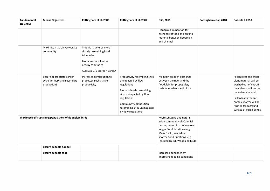
101
Fundamental Objective
Means Objectives Cottingham et al, 2003 Cottingham et al, 2007 DSE, 2011 Cottingham et al, 2018 Roberts J, 2018
Floodplain inundation for exchange of food and organic material between floodplain and channel
Maximise macroinvertebrate community
Trophic structures more closely resembling local tributaries
Biomass equivalent to nearby tributaries
Ausrivas O/E scores = Band A
Ensure appropriate carbon cycle (primary and secondary production)
Increased contribution to processes such as river productivity
Productivity resembling sites unimpacted by flow regulation;
Biomass levels resembling sites unimpacted by flow regulation;
Community composition resembling sites unimpacted by flow regulation;
Maintain an open exchange between the river and the floodplain for propagules, carbon, nutrients and biota
Fallen litter and other plant material will be washed out of cut-off meanders and into the main river channel.
Fallen leaf litter and organic matter will be flushed from ground surface of inside bends.
Maximise self-sustaining populations of floodplain birds Representative and natural avian community of: Colonial nesting waterbirds, Waterfowl: longer flood durations (e.g. Musk Duck), Waterfowl: shorter flood durations (e.g. Freckled Duck), Woodland birds
Ensure suitable habitat
Ensure suitable food Increase abundance by improving feeding conditions

102
Fundamental Objective
Means Objectives Cottingham et al, 2003 Cottingham et al, 2007 DSE, 2011 Cottingham et al, 2018 Roberts J, 2018
Ensure suitable life stage queues
Increase abundance by improving recruitment conditions
Achieve successful recruitment in as many years as possible
Maximise self-sustaining populations of turtles
Maximise self-sustaining populations of platypus
Maximise structural complexity and diversity of floodplain vegetation, including wetlands
Reinstate more natural connectivity to wetlands
Connection of floodplain ecosystem components, including grasslands, woodlands, permanent and temporary wetlands
Flood regime has all the elements of a natural floodplain, including - Seasonality - Frequency – Duration
Flood regime has all the elements of a natural floodplain
Connection of floodplain ecosystem components, including grasslands, woodlands, permanent and temporary wetlands
Wetland vegetation will go through successive phases of aquatic and amphibious development, abundance and then senescence with drawdown, followed by terrestrial non-woody species once dried out.
Maximise diversity of over-, mid-, and under-story vegetation
Increase the extent and diversity of aquatic vegetation
Maintain forest and forb vegetation currently present in wetlands and backwaters
Maximise structural complexity and diversity of bank vegetation
Maximise functional diversity of bank species
Maintain diversity, continuity and cover
Persistent cover of terrestrial grassy vegetation (flood sensitive) maintained over the upper part of the river bank (equivalent to natural flow percentiles where bank inundation frequency and duration have not changed
Maintain a spatially variable fringe of emergent or amphibious macrophytes at the water line and low channel levels –littoral edge
A littoral fringe of non-woody emergent or amphibious plants will be present at the toe of bank in summer – autumn at most favourable sites, in

103
Fundamental Objective
Means Objectives Cottingham et al, 2003 Cottingham et al, 2007 DSE, 2011 Cottingham et al, 2018 Roberts J, 2018
under the current or historic flow regime)
Reduced cover of terrestrial grassy vegetation (flood sensitive) for lower parts of bank that fall below the threshold (flow percentile where natural duration of inundation is approximately equal to historic)
Maintain community composition that is predominantly native species (notionally at least 75% by cover).
Reverse and prevent further encroachment of terrestrial shrubs and trees (i.e. distribution of plants beyond their normal range).
Protect vigour of trees in existing River Red Gum woodland established on inset benches.
Restrict terrestrial vegetation to upper parts of the river bank
Encourage naturally dynamic vegetation cover on in-channel benches and bars -i.e. to allow woody and non-woody vegetation to establish and persist (periodically, not indefinitely)
years with extended low flows.
Patches of non-woody amphibious plants (non-woody species) will be present and abundant on low-lying benches, in some years.
A ground cover dominated by perennial herbs and/or graminoids will persist on favourable sites on lower river bank
Reduce extent and impact of weeds
Avoid conditions that favour significant riparian and aquatic weeds known to occur in the area (e.g. Arrow-head Sagittaria).
Ensure social and community needs of the river are met (including fishing, boating, swimming and ceremonial uses)

104
Fundamental Objective
Means Objectives Cottingham et al, 2003 Cottingham et al, 2007 DSE, 2011 Cottingham et al, 2018 Roberts J, 2018
OTHER Increase the diversity and distribution of amphibian species

105
Appendix C: Workshop 2 Stakeholder development of conceptual models Workshop 2 Runsheet and Participant List
Kaiela (Lower Goulburn) River Environmental Flows Study Workshop 2 (of 4) Agenda
Workshop Date: Wednesday 11th December, 2019
Location: The Connection Shepparton, 7287 Midland Hwy, Shepparton 3630
Aims:
• review the objectives and performance measures from Workshop 1 • develop and discuss conceptual (cause-and-effect) models for each of the fundamental objectives (from above)
Agenda
Time Agenda item
9.45 Coffee and tea on arrival
10.00 Acknowledgement of Country (Avril)
Introductions (brief) and housekeeping
10.10
Workshop context and recap
1. What did we do in Workshop 1? (Avril) 2. What’s the scope for this workshop? (Libby Rumpff, powerpoint)
10.30 Reviewing the problem context, fundamental objectives and performance measures (from Workshop 1 - Libby)
- Use powerpoint and print outs with comment boxes so participants can make direct edits.
- Structure this with ~10 mins spent discussing each, plus 5 mins to make notes, and MU team can look at and speak to at end of day if needed. Note if they want to change performance measures this can be noted and done in the group break outs, but they need to discuss it with a facilitator who might have to make a call if there isn’t agreement.
11.15 Morning tea (15mins)
11.30 Libby – lead a discussion where each expert gets 5 mins to present a first-cut of their ecological cause-and-effect model(s), plus 5 mins questions from participants, reminding everyone they get a chance to work on this further. Libby to remind of scale for model and performance measure:
- Fish – large and small bodied (Dave and Wayne), - Vegetation – bank and floodplain (Kay) - Platypus (Melody) - Turtles (who?) - Macroinvertebrates (Vin)
Talk through social model, and why we have a macroinvert model presented (i.e. underpins many other models)

106
12:30 Group exercise – adding some detail to the cause-and-effect models, including a social model. Participants work with a model/value of their choosing (i.e. fish, platypus etc). Each group has a facilitator, whom will have a handout with instructions. Key tasks:
- What are the key drivers and threats to the ecological objectives? - Any competing hypotheses?
Step 1: For the value and performance measure (i.e. at scale) draw the conceptual model on butchers paper. Facilitator to judge from the group the expertise available, as to whether you work from the expert model or develop afresh. Noting many community members may choose to work with the social model.
• REMEMBER: - You are Producing a generic conceptual model that should be applicable across the
lower Goulburn. - Try to identify the most important variables that may impact on a decision to release
water (or not) for this performance measure, rather than produce a detailed model - If there is disagreement on the model structure, draw >1 models. - Note, if the expert model is really complex, try focus the group on the 5 key factors
driving the performance of the value, and if necessary work from there (i.e. start simple but don’t force it because they will address this in Step 2 after lunch!).
- Do not include flow management or other actions at this stage. - Get participants to be specific about the variables (e.g. rather than allowing ‘climate
change’ in a model, ask what specifically about climate change is the driver? Is it frequency of droughts, magnitude of droughts etc etc)
- If this is done in 45 mins, then continue to Step 2. You could do Step 1 and 2 together but I’m not sure there is time, and this is a better way not to get lost.
1.15 Lunch (30mins)
1.45 Group exercise (cont) – adding some detail to the cause-and-effect models. Key tasks:
- What are the (magnitude and direction of) key drivers and threats to the ecological objectives?
- How can we use flows to address these threats and drivers? - Note: What other management actions are important?
Step 2: Developing the influence diagrams into cognitive maps. - For each variable in the model, look at each accompanying child node and if the
relationship is in the same direction add a ‘+’ (e.g. as rainfall increases so does plant survival), and if in a different direction add a ‘-‘ (i.e. as fire frequency increases the survival of plants decreases). Use blue (+) or red (-) pens if possible. Libby will bring.
- For each ‘+’ or ‘-‘ indicate whether this is a strong, moderate or minor effect (i.e. +++, ++ or +, or vice versa with -)
- REMEMBER: You are asking about the average response of the performance measure across the Lower Goulburn. Think about the current period (i.e. 2019) as your starting point for each value, looking to the future.
- If uncertain, indicate range or + or – if possible, but the upper and lower bound should relate to the upper of the AVERAGE and lower of the AVERAGE (see above point), NOT absolute best and worst case across all sites in the Lower Goulburn.
- If really uncertain to the point where we don’t know if this is + or -, then specify as a green line.

107
Step 3: - Add in relevant management actions for each variable that can be influenced by
management. For timing o Start with flows!! Give detail on timing, location, amount, (affected model
variables) o If time, think about the other nodes that can be influenced by management. o Start with most influential variables (e.g. +++) and go from there (i.e. to
manage time) - Step 4: Think about: What data can we use? Are there key knowledge gaps?
3:30 Feedback from the groups: A spokesperson for each group has to answer the following questions, NOT present their model (because that’s hard given time available)
- What flows are required for the different models? - Any competing models/hypotheses? - Do we need to revise anything from Workshop 1? - What data can we use? Are there key knowledge gaps?
4.00 Wrap up for the day – what did we just do? (Libby, Avril, Meghan)
Next steps – how is the team translating the conceptual models into quantitative models? (Angus)
4.30 Finish for the day
10 List of participants
Name Organisation
1 Keith Chalmers
Kris Leckie
Victorian Environmental Water Holder,
Steering Committee
2. Andrew Shields Goulburn Murray Water, Steering Committee
3 Laura Caffrey DELWP, Steering Committee
4 Corey Walker Yorta Yorta, Steering Committee
5 Daniel Lovell GB CMA, Steering Committee
6 Simon Casanelia GB CMA, Steering Commitee
7 Steven Threfall Community Member, Goulburn EWAG
8 Russell Pell Community Member, Goulburn EWAG
9 Rob Asplin Community Member, Goulburn EWAG
10 Ian Gibb Community Member, Goulburn EWAG
11 John Pettigrew GVEG representative, Goulburn EWAG
12 Rolf Weber Community, Turtles Australia
13 Sean Kelly Commonwealth Environmental Water Holder, Goulburn EWAG

108
14 Ross McPherson Community
15 Alejandro Voysest Taungurung, Goulburn EWAG
16 Meg Pethybridge RiverConnect Project Officer
17 Craig Winnell Community member
18 Angus Webb The University of Melbourne, Goulburn River LTIM Team, Scientific Panel
19 Vin Pettigrove RMIT, Goulburn River LTIM Team, Scientific Panel
20 Mike Grace Monash University, Goulburn River LTIM Team, Scientific Panel
21 Kaylene Morris ARI, Goulburn River LTIM Team, Scientific Panel
22 Wayne Koster ARI, Goulburn River LTIM Team, Scientific Panel
23 Geoff Vietz Streamology, Goulburn River LTIM Team, Scientific Panel

109
Model Development from Workshop 2 to final Netica Model Structures This appendix briefly presents the model development for each of the fundamental objectives. This highlights how models were refined following the conceptual model building workshop in December 2019. We have attempted to justify significant changes to the structure of models and document the thinking of technical experts for their individual subject areas.
1. Fish Models
• While the objectives from Workshop #1 focused on small bodied and large bodied native fish populations, the model developed in Workshop #2 focused on the development of a self-sustaining full fish assemblage. This approach focused on three life-history groupings (opportunistic, equilibrium and periodic. This was done based on conversations within the workshop on how to differentiate between flow requirements for specific fish species.
• This original model had three primary groupings for drivers- habitat, recruitment/growth and movement within and outside of the system. The eventual models developed were divided between recruitment, survival and movement. This development was based on conversations with Wayne Koster and trying to align the conceptual model from the workshop with his model (sent to us in January after the workshop was complete, see Figure 43 below).
• The model in Figure 43 was not well suited for population through expert elicitation and was dissimilar from the model developed during the workshop, but we wanted to ensure that we captured both thought processes in our eventual model.
• While there are many commonalities in drivers between the three life-history groupings, it was decided that lumping them together was not well suited to the Bayesian models. Three separate models were then developed for fish for each life-history grouping.
• Models were refined through conversations with David Crook and Wayne Koster. Steps were taken to simplify the model where possible and complementary management activities were removed from the final models.
• Summary of other key changes to the models: o Avoidance of blackwater events in the original model changes to maintaining water quality for refugia in final o Water quality refugia linked to water depth, temperature and dissolved oxygen through development of statistical relationships
using historic data o Primary productivity removed from model, as it is included in the macroinvertebrate model and does not feed directly into drivers
for fish populations o Using macroinvertebrates as the primary food source in all three fish models ignores species that may be herbivorous (smaller
opportunistic species) or those that eat smaller fish (such as the Murray Cod)
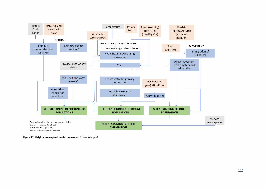
110
Figure 22: Original conceptual model developed in Workshop #2

111
Figure 23. Conceptual model from Wayne Koster emailed to Unimelb team in January 2020

112
Figure 24. Final Bayesian model for opportunistic fish

113
Figure 25. Final Bayesian model for equilibrium fish

114
Figure 26. Final Bayesian model for periodic fish

115
2. Bank Vegetation • Figure 6 below shows the conceptual model that was developed for bank vegetation in Workshop #2. This original model has three zones of
vegetation, the upper bank, mid-bank and littoral. There are many complementary drivers, including trampling/herbivory, logging and weed cover. There are only a limited number of flow related drivers, flow velocity and prolonged summer inundation. Due to the time limitations of the workshop, this model was not developed in explicit detail
• Conversations in January-March 2020 with Kaylene Morris fleshed out the vegetation model. It was decided that flows only have a limited influence on upper bank vegetation. Two vegetation models were developed for this project, mid bank and littoral vegetation. Figures 7 and 8 below shows the mid bank and littoral vegetation models updated with Kaylene Morris’s consideration. There is a detailed description of why flow drivers are included for each model. This was communicated to the Unimelb team in February 2020.
• Figures 9 shows the final Bayesian models used for the mid bank and littoral vegetation. • Below is a brief summary of the key changes to the model based on conversations with Kaylene Morris
o Trampling/herbivory and weeds were removed as complementary drivers as they are not a strong influence o Erosion was summarized as bank stability and linked to the geomorphic model o Prolonged summer flow (primarily IVTs) has been given more detail and described as “summer flow effect” o Many flow components have been added to the model and seed availability has been given a more precise definition as deposition
and retention (building seed banks). o Germination and establishment and reproduction of extant vegetation were added to the model

116
Figure 27. Conceptual model developed during Workshop #2

117
Figure 28: Documentation of Kaylene Morris' conceptual model and thought process for mid bank vegetation

118
Figure 29: Documentation of Kaylene Morris' conceptual model and thought process for mid bank vegetation

119
Figure 30: Bayesian model developed for mid bank and littoral vegetation. Note that the link between Autumn fresh and non-summer flows is NOT present in the littoral model

120
3. Floodplain Vegetation • Figure 10 below shows the conceptual model that was developed for floodplain vegetation in Workshop #2. There are several
complementary measures such as illegal logging and trampling/herbivory. Environmental factors such as bushfire and precipitation were also included
• Conversations from January-March 2020 with Kaylene Morris significantly changed this model, as it does not include some of the primary flow drivers and many of the relationships for floodplains are extremely uncertain. Figure 11 shows a refined version of the floodplain model sent to the Unimelb team in February by Kaylene Morris. This version of the model eliminated some of the less important complementary drivers and sought to simplify some of the relationships in the model and express them in the appropriate terms.
• Figure 12 shows the final Bayesian model used for the floodplain vegetation. • Below is a brief summary of the key changes to the model based on conversations with Kaylene Morris
o While illegal logging was kept, trampling/herbivory and weeds were removed as complementary drivers as they are not a strong influence
o Erosion was summarized as bank stability and linked to the geomorphic model o Environmental drivers that cannot be controlled in any way were removed from the model o “Entrapment and transport” and “germination and establishment” were added to the model and linked to the appropriate flow
drivers. These nodes took the place of some nodes in the original model.

121
Figure 31: Conceptual model for floodplain vegetation developed in Workshop #2

122
Figure 32: Conceptual model from Kaylene Morris in February 2020

123
Figure 33: Final quantitative Bayesian model for floodplain vegetation

124
4. Platypus • Figure 13 below shows the conceptual model that was developed for platypus in Workshop #2. There were three primary drivers in this
model, body condition, breeding, and recruitment. All other factors fed into these three primary drivers. There were a limited number of flow drivers with a focus on winter flows. Several of the drivers were environmental factors that were modeled as means objectives (ie: macroinvertebrates, bank stability, etc).
• The model was refined through conversations with Melody Serena from December 2019-May 2020, though this primary structure was never adjusted in a significant way.
• Figure 14 shows the final Bayesian mode used for platypus • Below is a brief summary of the primary changes to this model
o Breeding and recruitment were combined and defined as reproduction to simplify the model as there was a direct linkage between them. We believe this still accurately captures this process.
o Burrow habitat was originally linked to breeding and is now linked to reproduction o Macroinvertebrate abundance is throughout the year and linked directly to body condition and reproduction o Simplification of the drivers feeding into forage habitat, including removal of primary production as this influence
macroinvertebrate abundance

125
Figure 34: Conceptual model for platypus developed in Workshop #2

126
Figure 35: Final Bayesian model for platypus

127
5. Turtles • Figure 15 below shows the conceptual model that was developed for turtles in Workshop #2. Similar to platypus, there were three primary
drivers in this model, body condition, egg laying, and recruitment. There were a limited number of flow drivers- primarily overbank flows connecting anabranches and wetlands and spring bankfull flows related to nesting. Fox population played a large role in this model.
• The model was refined through conversations with Katie Howard from December 2019-May 2020, though this primary structure was never adjusted in a significant way. Katie Howard did propose that fox population should be linked to body condition and nesting habitat as well as egg laying and recruitment. Additionally, she proposed that macroinvertebrate population be connected to recruitment.
• Figure 16 shows the final Bayesian mode used for turtles • Below is a brief summary of the primary changes to this model
o Egg laying and recruitment were combined and defined as reproduction to simplify the model as there was a direct linkage between them. We believe this still accurately captures this process.
o Nesting habitat was originally linked to breeding and is now linked to reproduction o Fox population is linked to reproduction and final population, however we are aware that fox presence influences almost every
intermediate node in the model. It was decided that it influenced these two nodes most highly. Anything other than a small fox population has an enormous effect on the population, so we think this has been accurately captured
o Simplification of the drivers feeding into forage habitat, including removal of primary production as this influence macroinvertebrate abundance

128
Figure 36: Conceptual turtle model developed in Workshop #2

129
Figure 37: Final Bayesian model for turtles
Relevant flow components and existing knowledge provided to experts during expert elicitation Previous environmental flow studies have recommended a range of standard environmental flow components. The following provides and indication of the types of flow ranges that provide different flow events in the Kaiela (Business case).

130
• Base flows (or low, in-channel flows) that maintain aquatic habitat for fish, plants and invertebrates. Base flows comprise long-term seasonal flows and are usually delivered throughout the year as low volume (<1,000 ML/day at Shepparton) surface flows.
• In-channel fresh events are small-to-medium flow events (up to 8,500 ML/day at Shepparton) which inundate benches within the river channel, replenish soil water for riparian vegetation, provide cues for fish spawning and access to a diversity of habitat for aquatic biota. They are relatively short in duration (up to 14 days) and occur in most years, or possibly multiple times within a year.
• Bank-full flows are the larger flow events (up to 14,000 ML/day at Goulburn Weir) that fill the river channel and may inundate flood-runners in low lying areas of the floodplain. These flows are important for maintaining bed diversity, native fish recruitment and colonisation, regeneration of native riparian species and to retain natural seasonality for macroinvertebrate life stages.
• Overbank flows are the larger flow events that fill the river channel and low parts of the floodplain. They are important for a range of floodplain processes to occur e.g. healthy wetland systems that support fish and waterbird breeding, as well as the transfer of food and organic material that support productive instream foodwebs (MDBA, 2014; GBCMA, 2015).
Figure 38: Maximum velocity at vegetation transects for McCoy’s Bridge

131
Table A. 1 McCoys Bridge habitat area results (Source: LTIM report 2020)
Flow (ML / day)
Flow (m3/s)
Mean velocity (m/s)
Wetted area (m2)
Area of pools > 1.0 m (m2)
Area of pools > 1.5 m (m2)
Area of slackwater habitat (D < 0.5 m, V < 0.05 m/s) (m2)
No. patches slackwater habitat
Mean patch size of slackwater habitat (m2)
Area bed shear > 0.97 N/m2 (1 mm sediment mobilised)
Area bed shear > 1.94 N/m2 (2 mm sediment mobilised)
Bench area inundated (m2)
Change in velocity per ML/day change in flow (m/s/ML/day)
High Velocity (99%) (m/s)
300 3 0.10 24,875 14,048 9,769 3,659 93 39 2,082 1,616 - 0.000320 0.68
500 6 0.13 26,741 15,179 10,804 3,456 101 34 3,104 2,193 - 0.000184 0.78
1,000 12 0.20 29,662 17,752 13,723 2,756 130 21 6,806 3,306 113 0.000127 0.60
2,000 23 0.24 33,829 24,461 17,993 3,066 183 17 10,422 2,609 1,701 0.000041 0.51
3,000 35 0.27 36,988 29,541 23,902 2,004 223 9 14,777 3,613 3,330 0.000037 0.56
4,000 46 0.31 38,408 32,475 28,490 1,450 249 6 18,910 4,541 3,692 0.000032 0.60
5,000 58 0.33 39,601 35,588 31,401 1,292 273 5 22,021 5,781 3,809 0.000028 0.63
6,000 69 0.36 40,662 37,290 34,215 1,267 290 4 23,936 8,149 3,846 0.000023 0.65
7,000 81 0.38 41,863 38,455 36,484 1,320 284 5 25,750 10,312 3,855 0.000020 0.66
8,000 93 0.39 43,058 39,495 37,875 1,390 310 4 26,972 13,100 3,855 0.000015 0.69
10,000 116 0.42 45,636 41,468 39,706 1,787 287 6 29,022 18,397 3,855 0.000014 0.73
12,000 139 0.44 48,098 43,420 41,536 1,794 270 7 30,056 20,958 3,855 0.000011 0.79
15,000 174 0.48 51,096 46,397 43,969 1,647
32,517 24,558 3,855 0.000012 0.87
18,000 208 0.52 53,226 48,757 46,412 1,531
34,492 27,864 3,855 0.000013 0.95
20,000 231 0.54 54,495 50,277 47,803 1,465
35,481 29,256 3,855 0.000011 0.99

132
Figure 39: Reach at Wyuna: wetland inundation with discharge: total and for each vegetation class (Streamology, 2017)
Figure 40: Reach at McCoys Bridge: wetland inundation with discharge: total and for each vegetation class (Streamology, 2017)

133
Figure 41: Reach at Loch Gary: wetland inundation with discharge: total and for each vegetation class (Streamology, 2017)
Figure 42: Reach at Darcys Track: wetland inundation with discharge: total and for each vegetation class (Streamology, 2017)

134
Figure 43: Reach at Murchison: wetland inundation with discharge: total and for each vegetation class (Streamology, 2017)
Figure 44: Reach at Moss Road: wetland inundation with discharge: total and for each vegetation class (Streamology, 2017)

135
Figure 45: HECRAS output river cross sections Flow = 470 ML/d

136
Figure 46: HECRAS output river cross sections Flow = 940 ML/d
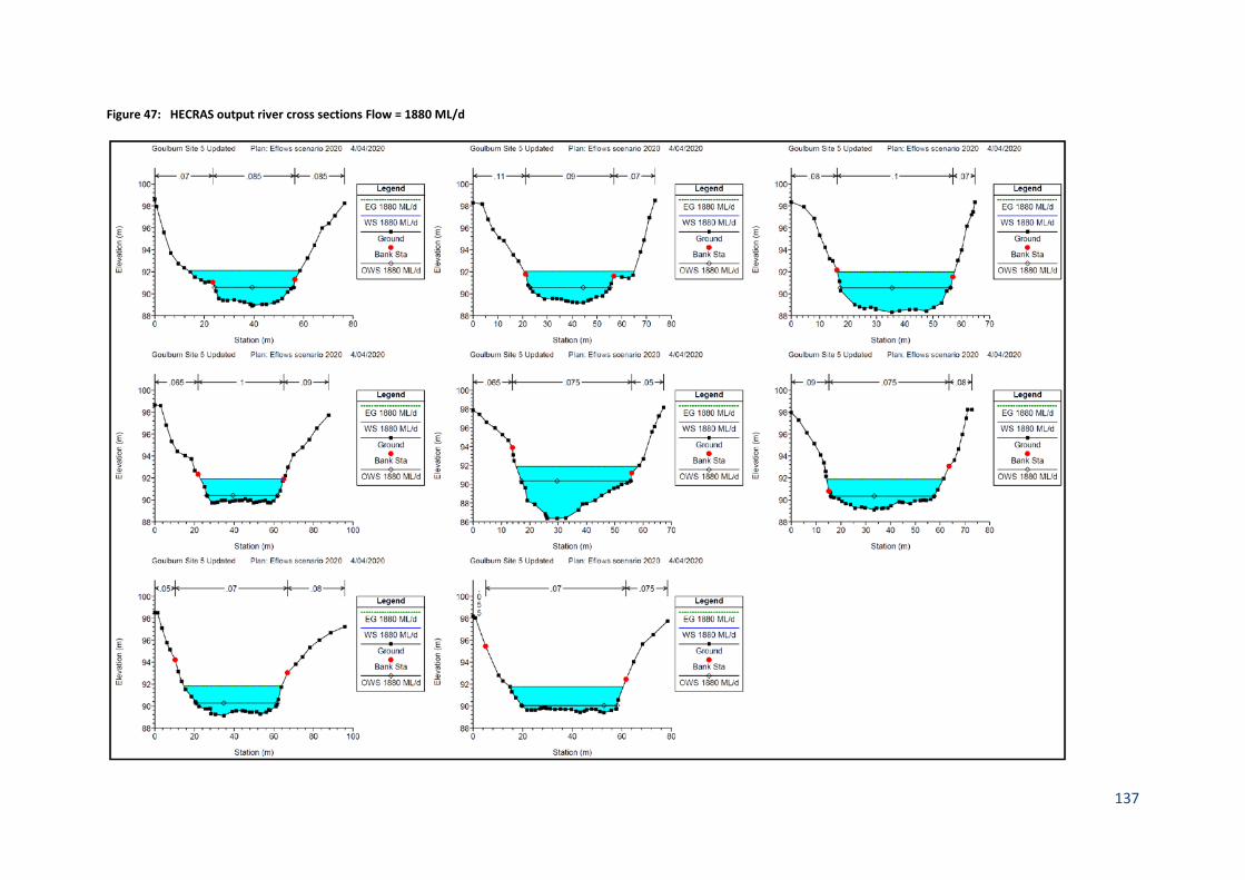
137
Figure 47: HECRAS output river cross sections Flow = 1880 ML/d

138
Figure 48: HECRAS output river cross sections Flow = 8,400 ML/d

139
Appendix D: Ecological models The sections below describe the final ecological model for each endpoint. Details on their construction is included in Appendix C.
Floodplain vegetation The Lower Goulburn River Floodplain supports a range of flood-dependent vegetation communities including river red gum (Eucalyptus camaldulensis) open forest woodland. Smaller areas of grey box (E. microcarpa) open forest woodland with associated yellow box (E. melliodora), white box (E. albens) and black box (E. largiflorens) occur on higher parts of the floodplain (DEWHA 2009).
The model shown in Error! Reference source not found. below represents the key flow and non-flow drivers that influence vegetation dynamics that underpin the fundamental objective “Complexity and Cover of Floodplain Vegetation”. Model components are detailed below.
Overbank flows: Overbank flows provide inundation for vegetation across the floodplain. The required frequency, depth and duration of inundation varies among floodplain and wetland vegetation assemblages. This model does not capture this complexity but represents the key role that overbank flow events and other non-flow drivers have on vegetation dynamics.
Tributary inputs: Overbank flows provide water and nutrients for floodplain and wetland vegetation. Flood waters can also supply seeds and vegetative fragments (collectively propagules) from source populations across the floodplain. The number and diversity of plant propagules supplied by overbank flows is expected to be higher when flooding arises from tributary inputs. As tributary inputs result from rainfall events that help to flush propagules into the stream network, they are likely to carry more propagule that flows released from dams. The importance of tributary inputs for propagule supply depends on the condition of tributaries.
Excess litter: Overbank flows also help to remove accumulated plant litter which at high levels can inhibit germination and establishment. Although the removal of accumulated litter is an important process to include in the model, the transport of carbon within floodplain systems is a complex and dynamic process and relationships between flow magnitude and the amount of carbon transported among different floodplain features in the Lower Goulburn River is currently not well understood. There are likely to be flow thresholds that need to be reached before accumulated carbon is flushed from wetlands.
Cool Fire: Cool fires can provide an alternative means to manage excessive litter accumulation, particularly when overbank flooding has not occurred. Fires must not be so severe that mature trees are killed.
Rainfall: The level of longer-term rainfall in the region may help some perennial plants persist between flood events and can also increase the duration of wetland inundation following overbank flows.

140
Logging: Logging of dead wood reduces important structural features that provide habitat for fauna. If mature live trees are logged this not only reduces habitat structure but removes a supply of seeds limiting regeneration.
Antecedent vegetation cover: Germination and establishment of plants in responses to overbank flow will be influenced by the condition of vegetation. Where vegetation is in good condition there is likely to be a good supply of propagule held in soil or aerial seed banks or produced seasonally. Where vegetation is in poor condition the supply of propagules will be reduced and plant establishment will be more reliant on the arrival of propagules from outside the system.
In the model, the relationship between High/Overbank flow and inundation was populated using a 2017 analysis by Streamology Pty Ltd, while all other relationships were populated using the expert opinion elicitation process.

141
Figure 49. Overall CPN model for floodplain vegetation developed in Netica. Drivers and outcomes are presented as probabilities, with the ‘belief bars’ in each node summing to 100%. For this example, with all drivers in neutral (i.e. all probabilities equal within each node), the probability of Floodplain Vegetation being in Good condition is 17.7%, Average condition 41.5%, and Poor condition 40.8%. All the model diagrams below are interpreted in the same way.

142
Figure 50 below presents the best scenario for the floodplain vegetation model. In this model, there is a 50000 ML/day overbank flow event with 67-100% of this flow coming from tributaries. These are the flow drivers within the model that are connected to environmental flows and the catchment management authority’s environmental watering plan. Controlling logging is a complementary management practice that can be recommended by the catchment management authority in conjunction with other agencies. This is true of the application of controlled cold fire as well.
Figure 50. Outcome when all driving elements are best possible for floodplain vegetation (high overbank flows with large proportion coming from tributaries, no logging within floodplain, good antecedent condition and high rainfall year).

143
High overbank flows are essential for obtaining floodplain vegetation of at least an average rating. When High overbank flows is the only node being manipulated, there is a large impact on the germination and establishment node. Table 18 below outlines the changes to vegetation condition when only the high overbank flow node is changed. While having an extremely high flow of 50000 ML/day does not guarantee good floodplain vegetation condition, having lower flows of only 14000 ML/day greatly increases the likelihood of poor vegetation condition. The model does not address the question of how often overbank flows are required to maintain prevent loss of floodplain vegetation. A sequence of years with no overbank flows would see the probability of a poor outcome rising with each year of no flooding. For a comparison of flow components and outcomes for most favourable and least favourable scenarios for floodplain vegetation refer to Table 19 below.
A sensitivity analysis was performed on the final node, Floodplain Vegetation Complexity and Cover, to ascertain which of the drivers have the greatest impact on the final node. In this analysis, we found that logging had the greatest impact on floodplain vegetation, indicating that even the best flow conditions will have a limited impact if logging is still taking place. The next most important drivers were germination and establishment, inundation and high overbank flows.
Table 18. Implications for Floodplain vegetation health based on changes to high/overbank flow node
High/Overbank Flows Floodplain Vegetation Condition Good Average Poor 50000 ML/day 22.3 45.0 32.7 40000 ML/day 21.6 45.4 33.0 30000 ML/day 18.6 43.9 37.5 20000 ML/day 13.5 37.3 49.3 14000 ML/day 12.6 35.7 51.6
Table 19. Comparison of flow components and outcomes for most favourable and least favourable scenarios for floodplain vegetation
Scenario Flow Components Floodplain Vegetation Condition
Proportion Tributaries High Overbank Flow Good Average Poor
Best Between 67 and 100% 50000 ML/D 22.5 45 32.5
Worst Between 0 and 33% 14000 ML/D 12.6 35.7 51.7
Note: For these scenarios, all non-flow drivers were held in even distributions among possible states. It should be clear that in some models, non-flow drivers have a greater influence over model outcomes than flow drivers. This is not captured in this summary table, but described in detail in the model write up

144
Littoral and mid bank vegetation Bank vegetation generally refers to vegetation on the sides of a river channel and extends from the toe of the bank to the top of the bank. The depth and duration of inundation produced by a flow event varies along the bank face (Figure 51).
Figure 51. Schematic showing different inundation experienced by location on the bank face.
A single conceptual model was developed for the structural complexity of bank vegetation with a focus on mid-bank and littoral regions. While there is a single conceptual model for both regions, the conditional probability networks for each region were populated separately, generating two distinct models. The lower bank is defined hydrologically as the region of the bank inundated at 7500 ML/day (Roberts, 2018). For the purposes of this study, the littoral zone is defined as the lowest part of the riverbank. Flow range for this feature currently ranges from lowest flows of 750 to 1100 ML/d (Roberts, 2018).
Vegetation on the mid bank varies from species intolerant of prolonged inundation at the boundary between the mid and upper bank such as Poa labillardierei (Common tussock grass), to species tolerant of flooding but requiring flood recession over summer, such as Pasaplidium jubiflorum and Carex tereticaulis. Some species tolerate a range of hydrological conditions and are more widely distributed across the elevation gradient such as Persicaria prostrata (Cottingham et al, 2018).
Species at the lower elevations including the littoral zone are adapted to tolerate more frequent inundation and are less tolerant of drying. These species include a range of sedge and rushes (Cyperus eragrostis, Cyperus exaltatus, Juncus spp.) and forbs including, Persicaria hydropiper, Alternanthera denticulata and Centipeda cunninghamii (Cottingham et al., 2018).
The model shown in Figure 52 represents key flow and non-flow drivers that influence vegetation dynamics that underpin outcomes for mid-bank vegetation. Model components are detailed below.
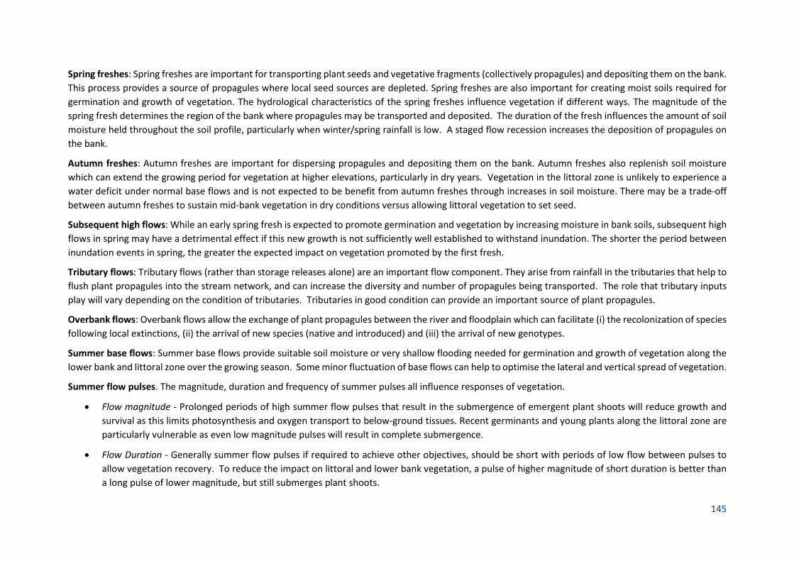
145
Spring freshes: Spring freshes are important for transporting plant seeds and vegetative fragments (collectively propagules) and depositing them on the bank. This process provides a source of propagules where local seed sources are depleted. Spring freshes are also important for creating moist soils required for germination and growth of vegetation. The hydrological characteristics of the spring freshes influence vegetation if different ways. The magnitude of the spring fresh determines the region of the bank where propagules may be transported and deposited. The duration of the fresh influences the amount of soil moisture held throughout the soil profile, particularly when winter/spring rainfall is low. A staged flow recession increases the deposition of propagules on the bank.
Autumn freshes: Autumn freshes are important for dispersing propagules and depositing them on the bank. Autumn freshes also replenish soil moisture which can extend the growing period for vegetation at higher elevations, particularly in dry years. Vegetation in the littoral zone is unlikely to experience a water deficit under normal base flows and is not expected to be benefit from autumn freshes through increases in soil moisture. There may be a trade-off between autumn freshes to sustain mid-bank vegetation in dry conditions versus allowing littoral vegetation to set seed.
Subsequent high flows: While an early spring fresh is expected to promote germination and vegetation by increasing moisture in bank soils, subsequent high flows in spring may have a detrimental effect if this new growth is not sufficiently well established to withstand inundation. The shorter the period between inundation events in spring, the greater the expected impact on vegetation promoted by the first fresh.
Tributary flows: Tributary flows (rather than storage releases alone) are an important flow component. They arise from rainfall in the tributaries that help to flush plant propagules into the stream network, and can increase the diversity and number of propagules being transported. The role that tributary inputs play will vary depending on the condition of tributaries. Tributaries in good condition can provide an important source of plant propagules.
Overbank flows: Overbank flows allow the exchange of plant propagules between the river and floodplain which can facilitate (i) the recolonization of species following local extinctions, (ii) the arrival of new species (native and introduced) and (iii) the arrival of new genotypes.
Summer base flows: Summer base flows provide suitable soil moisture or very shallow flooding needed for germination and growth of vegetation along the lower bank and littoral zone over the growing season. Some minor fluctuation of base flows can help to optimise the lateral and vertical spread of vegetation.
Summer flow pulses. The magnitude, duration and frequency of summer pulses all influence responses of vegetation.
• Flow magnitude - Prolonged periods of high summer flow pulses that result in the submergence of emergent plant shoots will reduce growth and survival as this limits photosynthesis and oxygen transport to below-ground tissues. Recent germinants and young plants along the littoral zone are particularly vulnerable as even low magnitude pulses will result in complete submergence.
• Flow Duration - Generally summer flow pulses if required to achieve other objectives, should be short with periods of low flow between pulses to allow vegetation recovery. To reduce the impact on littoral and lower bank vegetation, a pulse of higher magnitude of short duration is better than a long pulse of lower magnitude, but still submerges plant shoots.

146
• Summer pulses may provide short term benefit to vegetation higher up the bank by improving soil moisture, however long-duration summer pulses reduce bank stability and can result in bank slumping and compromise vegetation higher up the bank.
• Number of pulses - To support germination and early establishment of littoral and lower bank vegetation, delivering pulses at least 6 weeks following the recession of the spring fresh would increase the likelihood that recent germinants are able to reach a stage that is less vulnerable to summer pulses. A period of low flow for 12 weeks or longer would allow many plants that have established from seed to have matured and set seed, replenishing the soil seed bank and improving resilience. Although established littoral vegetation is more tolerant of flow pulses, several years of frequent summer pulses reduces opportunities for growth, which may limit vegetative spread, seed production and carbohydrate stores in below-ground structures. All these contribute to the resilience of vegetation and its ability to recover from unfavourable events.
Bank Stability: Bank stability is critical in the maintenance and establishment of bank vegetation. Where erosion occurs, vegetation may be uprooted and seeds washed away.
Antecedent condition: The state of vegetation strongly influences responses to flow components. This is most significant where vegetation has been lost because flows needed for re-establishment differ to the flows required to maintain established vegetation. Where vegetation is locally absent or in low abundance, aerial and soil seed banks are likely to be low and there will be a greater reliance on propagule arrival from source populations.
For the purposes of this model, flows have been separated into “summer” and “non-summer” flows. This is to acknowledge that in recent years, higher flow volumes due to IVTs have led to a generally negative impact on vegetation during summer months, while higher flows in other seasons are generally valuable and occur due to natural events or environmental releases to supplement natural tributary inflows.

147
Figure 52. Overall CPN model for mid-bank vegetation developed in Netica.
A best-case scenario was examined, as represented in Figure 53. In this scenario, the summer flow effect was set to mild and all the other flow drivers were set to their best possible conditions with maximum fresh volumes, high overbank flows, a high proportion of flows being supplied by tributaries. In addition, for this scenario the previous mid-bank vegetation condition was set as good. In this scenario it is extremely likely that mid-bank vegetation condition will be in good or average condition.

148
Figure 53. Outcome when all driving elements are best possible for mid-bank vegetation (high winter baseflow, spring and autumn freshes, high overbank flow, with a high proportion of these flows coming from tributaries, mild effects from IVTs and a good antecedent vegetation condition).
Certain drivers were examined in more detail and their influence on the model was isolated. This was done for the summer flows node, representing the influence of IVTs on the system. The summer flow effect node is influenced by the summer base flow, pulse magnitude, pulse duration and number of pulses. When all these parent drivers are set to their best states, the summer flow effect is likely to be moderate. When the situation is reversed, and all nodes are set to their worst states, counter-intuitively, the model predicts these effects to be mild. This stems from the expert elicitation process, in which the vegetation expert estimated that in all conditions that the summer flow effect would be mild. This plays out in the model as a control on the summer flow effect in which no conditions trigger severe summer flow effects, leaving them primarily in mild or moderate. However, this does not match our experience or data from the system, and we believe it to be caused by misinterpretation of some questions during the expert elicitation process. With this in mind, we manipulated summer flow effects directly for this scenario, rather than by manipulating the flow events that lead into this node. For a comparison of flow components and outcomes for most favourable and least favourable scenarios for midbank vegetation refer to Table 21 below. Subsequent to the analysis and sensitivity analysis, review comments suggested that the outcomes for summer flow effects, for mid-bank vegetation only, are not as surprising as we first perceived.

149
Higher summer flows can create bank moisture for mid-bank vegetation as long as the vegetation is not inundated for long periods. Under these conditions, a small positive effect of summer flows is not unreasonable.
A sensitivity analysis was performed on the final node, Mid-Bank Vegetation and Cover. We found that the most important driver for the model was the antecedent condition of the vegetation. When all nodes were held in a constant state, the influence of the antecedent condition was extremely strong. The next most important drivers were reproduction of extant vegetation and non-summer flows, which are highly related to one another as well. Additionally, bank stability was also highly influential on model outcome. While high overbank flows has a large impact on the deposition and retention of sediments on riverbanks, this impact is not carrying through to the final vegetation condition as other drivers have a higher impact.
Figure 54 below presents the overall model for littoral vegetation condition and coverage. The only structural difference between this model and the mid-bank vegetation model is that the autumn fresh flow driver is only connected to the deposition and retention node. As described above, the probability tables for this model were populated based on their own set of questions in which experts were explicitly asked to consider littoral vegetation.
Figure 54. Overall CPN model for littoral vegetation developed in Netica.

150
A best-case scenario was examined, as represented in Figure 55 below. In this scenario, the summer flow effect was set to mild and all the other flow drivers were set to their best possible conditions with maximum fresh volumes, high overbank flows, a high proportion of flows being supplied by tributaries. In addition, for this scenario the antecedent littoral vegetation condition was set as good as was the condition of bank stability. In this scenario it is extremely likely that the littoral vegetation will be in good or average condition. It is important to note that antecedent condition is the overwhelming driver for this model (similar to mid-bank vegetation above). For instance, if all drivers are held constant in their best state but the antecedent condition is changed to poor the littoral vegetation is extremely likely to be in poor or average condition (See Figure 55 below). Bank stability also has a large influence on the overall outcome when all states are held in their best possible conditions. If all states are held in their best possible conditions while bank stability is adjusted to poor, the probability for the littoral vegetation condition is almost evenly distributed between good, average, and poor conditions. This means that if conditions are primarily good for littoral vegetation, but bank stability is poor, it may be difficult to predict the condition of littoral vegetation.
Figure 55. Outcome when all driving elements are best possible for littoral vegetation (high winter baseflow, spring and autumn freshes, high overbank flow, with a high proportion of these flows coming from tributaries, mild effects from IVTs and a good antecedent vegetation condition, and good bank stability condition).

151
Certain drivers were examined in more detail and their influence on the model was isolated. This was done for the summer flows node, representing the influence of IVTs on the system. The summer flow effect node is influenced by the summer baseflow, pulse magnitude, pulse duration and number of pulses. When all these parent drivers are set to their best states, the summer flow effect is likely to be mild. When the situation is reversed, and all nodes are set to their worst states, these effects are likely to be moderate or severe. The influence of these drivers on the summer flow effect are stronger for littoral vegetation than for mid-bank vegetation. This is due to littoral vegetation and their location on the periphery of the water’s edge to slightly in-channel location. This means that heightened, sustained summer flows will have a greater impact on these species. A sensitivity analysis was performed on the reproduction of extant vegetation node, which is the child node of summer flow effects. We found that when all parent nodes were left in their distributed states, the most important influence on this node was bank stability. However, when summer flow drivers were shifted to their worst possible states causing the effect to be moderate to severe, summer flow effects became the most important driver of reproduction of extant vegetation. This indicates that if summer flow effects are moderate to severe, even if all other drivers are in their best state, then it is likely that reproduction of extant vegetation will be poor or average. This is reflected in the overall outcome for the final littoral vegetation node as well. For a comparison of flow components and outcomes for most favourable and least favourable scenarios for littoral vegetation refer to Table 21 below.
A sensitivity analysis was performed on the final node, Littoral Vegetation and Cover, to ascertain which of the drivers have the greatest impact on the model outcome We found that the most important driver for the model was the antecedent condition of the vegetation. When all nodes were held in a constant state, the influence of the antecedent condition was extremely strong, driving the outcome of the model. The next most important drivers were reproduction of extant vegetation, bank stability and summer flow effects. This is the main difference between this model and the mid-bank vegetation model. The condition of littoral vegetation is more highly dependent on bank stability and summer flow effects. While high overbank flows have a large impact on deposition and retention, this impact is not carrying through to the final vegetation condition as other drivers have a higher impact.
Table 20. Comparison of flow components and outcomes for most favourable and least favourable scenarios for midbank vegetation
Scenario Flow Components Midbank Vegetation Condition
High Overbank
Flows
Proportion Tributaries
Subsequent High Flows
Autumn Fresh Winter Baseflow Spring Fresh Good Average Poor
Best More than 25000
Between 67 and 100%
None 9900 ML/D 1800 ML/D 8400 ML/D 29.8 31.9 38.3
Worst None Between 0 and 33%
Under 8 weeks 4620 ML/D 470 ML/D 3920 ML/D 24.1 29.3 46.6

152
Note: For these scenarios, all non-flow drivers were held in even distributions among possible states. It should be clear that in some models, non-flow drivers have a greater influence over model outcomes than flow drivers. This is not captured in this summary table, but described in detail in each model’s description.
Table 21. Comparison of flow components and outcomes for most favourable and least favourable scenarios for littoral vegetation
Scenario Flow Components Littoral Vegetation Condition
High Overbank
Flows
Proportion Tributaries
Subsequent High Flows
Autumn Fresh Winter Baseflow Spring Fresh Good Average Poor
Best More than 25000
Between 67 and 100%
None 9900 ML/D 1800 ML/D 8400 ML/D 22.2 34.8 43.1
Worst None Between 0 and 33%
Under 8 weeks 4620 ML/D 470 ML/D 3920 ML/D 19.7 33.0 47.3
Note: For these scenarios, all non-flow drivers were held in even distributions among possible states. It should be clear that in some models, non-flow drivers have a greater influence over model outcomes than flow drivers. This is not captured in this summary table, but described in detail in each model’s description.
Platypus Figure 56 below shows the model structure for platypus. Platypus populations are governed by the antecedent population condition at the end of the previous year plus the success of reproduction during the current year. Reproductive success is a function of the provision of burrow habitat in which the young platypus are reared, and the ability for adult platypus to find sufficient food to maintain good body condition both prior to breeding and after the birth of the young.
Food availability is driven by the availability of forage habitat and macroinvertebrate abundance as the major food source. Foraging habitat is improved in rivers with high habitat complexity, and if the river’s connection to wetlands is good. Connection is facilitated by winter overbank and high flows.
Burrow habitat suitability is improved by high bank stability allowing the adults to build and maintain nesting burrows. Winter high flows provide a cue for lower-risk nest site selection by adults. The occurrence of bankfull and overbank flows in the period when juveniles are confined to burrows (from September through at least January) is predicted to result in widespread, catastrophic breeding failure due to nesting burrows being drowned out, though some

153
protection from briefly peaking high flows may be provided in the first half of juvenile development by the compacted soil ‘pugs’ routinely fabricated by mothers to block access to nesting burrows in this period.
Figure 56. Overall CPN model for platypus developed in Netica.
Figure 57 below presents the best flow scenario for the platypus population while non-flow drivers are left distributed among the different possible states. When flow drivers are in their optimal states, the platypus population is likely to be large or medium, with a 57.7% chance of being large. For a comparison

154
of flow components and outcomes for most favourable and least favourable scenarios for platypus population refer to Table 22 below. A sensitivity analysis was performed on the final node, Self-Sustaining Platypus Population, to ascertain which of the drivers have the greatest impact on the model outcome. We found that by far, the most important driver for the model was the antecedent population node. This reflects the long-lived nature of platypus populations. Populations will only shift slightly from year to year based on flow drivers, thus it will take a period of several years for these changes in flow to cascade through and affect the platypus population. The next most important node was reproduction, which is to be expected given that this is one of the immediate parent nodes for the final population. The next most important drivers were body condition and macroinvertebrate population respectively. Macroinvertebrate population was found to have a large impact on the final population outcome. This is most likely because it drives both body condition and reproduction. The least important driver in the model was late winter high flows.

155
Figure 57. Outcome when all flow drivers are the best possible for a self-sustaining platypus population (low winter and late winter overbank/high flows with lower relative flows in Sep-Jan).
Table 22. Comparison of flow components and outcomes for most favourable and least favourable scenarios for platypus population
Scenario Flow Components Platypus Population
Winter Overbank High
Flows
Late Winter High Flows
Sept to Jan Flows (in relation to Winter Flows)
Large Medium Small
Best 10500 ML/D 10500 ML/D 6000 ML/D 59.0 29.5 11.5
Worst 22500 ML/D 22500 ML/D 22500 ML/D 55.4 31.5 13.1
Note: For these scenarios, all non-flow drivers were held in even distributions among possible states. It should be clear that in some models, non-flow drivers have a greater influence over model outcomes than flow drivers. This is not captured in this summary table but described in detail in each model’s write-up.
Turtles Forage habitat combined with macroinvertebrate population are the key drivers that influence turtle body condition. Body condition influences the likelihood of breeding and egg production, essential for population persistence.
It is important that deep pools persist throughout the year as they provide important refuge and forage habitat. Forage habitat is also influenced by the condition of the littoral vegetation, and wetland connectivity, as food sources are present in different environments.
Winter high and overbank flows strongly influence the connectivity to wetlands within the riparian corridor. High flows fill flood runners that connect the main channel to wetland areas and turtles use these habitat corridors. This wetland connection is also a driver for nesting habitat
The provision of appropriate nesting habitat is essential for species persistence and is driven primarily by a relationship with bank stability. Banks need to be stable enough to support nests on the upper banks (above high water), but not so steep as to be inaccessible. Nesting habitat can be adversely impacted by high and overbank flows in Oct-Jan, as inundation of buried eggs will kill them.

156
Reproduction, describing the process from breeding to through to the appearance of juvenile turtles, is driven by nesting habitat and adult body condition with a strong negative influence from fox presence. Foxes will feed on eggs, juveniles and adults and negatively influence reproduction and the ultimate turtle population.
The ultimate fundamental objective, a self-sustaining turtle population, is driven by the antecedent turtle population and reproduction in the current year. A strong turtle population from a previous year needs to have appropriate reproductive opportunities to continue thriving in the present year. Fishing can negatively influence a turtle population through accidental bycatch in nets and by anglers.
Figure 58 below shows the overall Netica CPN model finalized following the expert elicitation workshop and subsequent conversations with Katie Howard, the selected expert. This model is highly influenced by drivers that are related to other modelled objectives (macroinvertebrate abundance, littoral zone vegetation condition, bank stability, and instream habitat complexity). The flow drivers are limited to overbank flows and late spring/early summer high flows. It is important to note that this analysis was done with the fox population set to small as having an evenly-distributed fox population had major impacts on the turtle population, even if every other driver was in its best possible state.

157
Figure 58. Overall CPN model for turtle population developed in Netica.

158
In Figure 59, all drivers of the model are set to the best possible combination for turtles. Note, while this provides a high likelihood of good forage habitat, wetland inundation, body condition and nesting habitat—reproduction may still be moderate. For a comparison of flow components and outcomes for most favourable and least favourable scenarios for turtle population refer to Table 23 below.
Figure 59. Outcome when all driving elements are the best possible for turtles (rare foxes and fishing, good bank stability, macroinvertebrates, habitat complexity, littoral zone vegetation and high winter flow event, no high summer event).

159
A sensitivity analysis was performed on the final node, Turtle Population, to ascertain which of the drivers have the greatest impact on the final node. In this analysis, we found that reproduction and fox population had the largest impact on the final outcome of the turtle population. Antecedent population had 10 times less influence on the final node. Reproduction was also strongly influenced by fox population, explaining why fox population has such a large effect on overall model performance. The second strongest impact on reproduction was from body condition.
Table 23. Comparison of flow components and outcomes for most favourable and least favourable scenarios for turtle population
Scenario Flow Components Turtles Population
Overbank Flows
Oct-Dec High Flows
Large Medium Small
Best 50000 ML/D None 41.6 41.1 17.3
Worst 14000 ML/D > 25000 ML/D 34.7 40.4 24.9
Note: For these scenarios, all non-flow drivers were held in even distributions among possible states, except fox population which was limited to small. It should be clear that in some models, non-flow drivers have a greater influence over model outcomes than flow drivers. This is not captured in this summary table but described in detail in each model’s write-up.
Fish Models The final model presented for the diverse fish assemblage looks significantly different from the original conceptual model developed during the workshop. The models presented below were constructed through an iterative process with the fish biologists associated with this project and represent a synthesis of the models. The conceptual model for a diverse fish assemblage has been split into three models, each representing a different functional group of fish species. This approach was used as it primarily based on reproductive traits that are often driven by flow requirements. This is only one way of many alternatives to divide the fish assemblage.
The three models presented below are extremely similar in most regards, and we will first outline the drivers and nodes that are common among the three models. Every population is influenced by three primary drivers, the survival, recruitment and movement of the population. Fish species must be able to spawn, survive through to adulthood and disperse within the catchment.
In these models, the number of fish that survive from one generation to the next (Survival) is a function of how many fish there are to begin with (antecedent population – i.e. the number of fish at the end of the previous year), and how good conditions are for survival. Survival is influenced by three drivers that are related to previously developed models including water quality, diverse instream habitat, and a healthy macroinvertebrate population. For survival, there

160
must be a food source, a diversity of places to hide and rest. Blackwater events must be kept at a minimum, as they negatively affect fish survival in all three fish groups.
Movement in all three populations is influenced by connectivity throughout the catchment and, for the periodic fish, to the larger Murray-Darling basin. In all three models, this connectivity is influenced by year-round baseflow and freshes to allow for and cue movement throughout the reaches. There is also a driver of late winter/spring high flows/bankfull which allow for large-scale migration within and beyond the boundaries of the catchment, but only for equilibrium and periodic species. For opportunistic species, this higher baseflows, overbank flows and freshes with appropriate timing provide connectivity to off-channel habitats.
Recruitment is present in all three models as drivers of overall population health but is significantly different among the three models.
Periodic Fish Model
Figure 60 shows the model for periodic fish species (i.e. golden and silver perch). In this model, spawning cues and macroinvertebrate populations are the primary drivers behind recruitment. Spawning is triggered by a fresh timed from Oct-Dec.
Figure 61 shows a best-case scenario when all drivers, both flow and non-flow, are set to their optimal condition. In this case, it becomes likely that the periodic fish population will be large or medium. Manipulating habitat diversity, macroinvertebrates and the antecedent condition, we see a large positive influence on the outcome of the final node. The model’s behaviour suggests that good performance for the periodic fish objective requires both flow and non-flow drivers to be in their optimal conditions. Flow drivers do not cause a significant shift in the final population outcome unless the other drivers are set to optimal condition and vice versa. For a comparison of flow components and outcomes for most favourable and least favourable scenarios for periodic fish refer to Table 24 below.

161
Figure 60. Overall CPN model for periodic fish population developed in Netica.

162
Figure 61. Outcome when all driving elements are the best possible for periodic fish population (high baseflow, bankfull flow, and fresh with optimal timings as well as complex habitat, good macroinvertebrate populations and a large antecedent population).

163
A sensitivity analysis was performed for the final node, Periodic Fish Population, to determine which drivers were the most influential on the overall model outcome. We found that recruitment and survival were the two most important drivers. These drivers were around twice as important as the movement (non-spawning related) driver, the third most influential node. Of the flow drivers, the most important was the fresh node. By examining the performance of the model in different scenarios, we found that the drivers within this model are extremely dependent on one another. For instance, the instream habitat diversity node is insignificant when all other drivers are in their worst states, but highly influential when all drivers are in their best states. Shifting habitat complexity from complex to simple in this scenario can cause the final population to shift from large to medium. Antecedent population, habitat diversity, and the combined effect of the flow drivers all demonstrate this behaviour. Macroinvertebrate population was highly influential in all scenarios.
Table 24. Comparison of flow components and outcomes for most favourable and least favourable scenarios for periodic fish population
Scenario Flow Components Periodic Fish Population
Baseflow High/Bankfull Flow Timing of Bankfull Fresh Timing of Fresh Large Medium Small
Best 1880 ML/D 22500 ML/D September 8400 ML/D November 19.6 41.9 38.5
Worst 470-752 ML/D 10500 ML/D July 3920 ML/D October 11.5 38.5 51.9
Note: For these scenarios, all non-flow drivers were held in even distributions among possible states. It should be clear that in some models, non-flow drivers have a greater influence over model outcomes than flow drivers. This is not captured in this summary table but described in detail in each model’s write-up.
Equilibrium Fish Model
The equilibrium fish (for example Murray and Trout cod) model has an extremely similar structure to that of the periodic fish with one key change. The main difference is that there is no spawning/movement node in the equilibrium model and there is instead a nesting conditions node. Nesting conditions is driven by variability in flow represented by the rate of the rise and fall and timing of the rise and fall nodes. A highly variable falling limb in a fresh can be detrimental for fish larvae. It is important to note that while macroinvertebrates are included as the main source of food in the equilibrium model, smaller (typically opportunistic) fish are also a source of food for the Murray Cod, a prominent equilibrium species.
Figure 62 below shows the final structure of the equilibrium fish model. In this scenario all drivers are left with even distributions among the possible states.
Figure 63 below presents the best flow scenario for the equilibrium fish population. In this scenario all of the flow drivers have been adjusted to their optimal states while the other drivers were left with even distributions. A high magnitude fresh is provided, there are high bankfull flows in September, the average baseflow magnitude is high, and the rate of rise and fall is slow. In this scenario, the equilibrium fish population is only slightly improved. When all drivers are set to their optimal state including non-flow drivers (habitat diversity, macroinvertebrates, and antecedent condition) the equilibrium fish population is very likely to be large to medium.

164
Figure 62. Overall CPN model for equilibrium fish population developed in Netica.
When the flow drivers are in their worst possible states and the non-flow drivers are left evenly distributed among their possible states, it is very likely that the equilibrium fish population will be small to medium. If the flow drivers are held in their worst-case states while the non-flow drivers are adjusted to their best states, the expected outcome of the final equilibrium population shifts to medium. This indicates that the model behaviour is more strongly influenced by non-flow drivers and the flow drivers are most important when other drivers are in their optimal states. For a comparison of flow components and outcomes for most favourable and least favourable scenarios for equilibrium fish refer to Table 25 below.

165
A sensitivity analysis was conducted on the final node to determine which drivers were the most influential. We found that the survival node was by far the most significant node in the model, almost three times as influential as the next most significant node, recruitment. After survival and recruitment, macroinvertebrates was the most influential driver of the final outcome. As expected, based on testing of various model scenarios, flow drivers were the least influential on ultimate model outcome. Of the flow drivers, baseflow had the most significant individual impact.
Figure 63. Outcome when flow elements are best possible for equilibrium fish population (high baseflow, bankfull flow and fresh, rate of rise and fall is slow and well timed). All non-flow drivers are left in even distributions.

166
Table 25. Comparison of flow components and outcomes for most favourable and least favourable scenarios for equilibrium fish population
Scenario Flow Components Equilibrium Fish Population
Baseflow High/Bankfull Flow Timing of Bankfull Fresh Rate of Rise/Fall Timing of Rise/Fall
Large Medium Small
Best 1880 ML/D 22500 ML/D September 8400 ML/D 50% of Recommendation
September 29.1 35.4 35.5
Worst 470-752 ML/D 10500 ML/D July 3920 ML/D 125% of Recommendation
December 17.2 37.2 45.7
Note: For these scenarios, all non-flow drivers were held in even distributions among possible states. It should be clear that in some models, non-flow drivers have a greater influence over model outcomes than fl drivers. This is not captured in this summary table but described in detail in each model’s write-up.
Opportunistic Fish Model
The opportunistic fish (such as Australian smelt) model is structurally similarly to the previous two fish models, with a few differences. The connectivity node from the previous model has been changed to connectivity cues within and is driven by depth and a fresh. This is to differentiate connectivity within the reach from connectivity to off channel habitat. The connectivity to off channel node is driven by a high/bankfull flow node and the timing of that flow. The structure of this model can be seen below in Figure 64. For this scenario, all drivers have been left with even distributions among the possible states. When all drivers are set to their optimal states including non-flow drivers, it is extremely likely that the opportunistic fish population will be large. For a comparison of flow components and outcomes for most favourable and least favourable scenarios for opportunistic fish refer to Table 26 below.
A sensitivity analysis was conducted on the final node to examine which drivers were the most influential of overall model behaviour. The findings were similar to those for equilibrium fish population in that survival was by far the largest driver of model outcome, followed by recruitment and macroinvertebrates. Movement and connectivity cues within channel were also highly influential on model outcome. Of the flow drivers, the most influential driver was the fresh. Antecedent condition was less influential in this model than in the other two fish models because these are short-lived species.

167
Figure 64. Overall CPN model for opportunistic fish population developed in Netica.

168
Table 26. Comparison of flow components and outcomes for most favourable and least favourable scenarios for opportunistic fish population
Scenario Flow Components Opportunistic Fish Population
Baseflow High/Bankfull Flow Timing of Bankfull Fresh Large Medium Small
Best 1880 ML/D 22500 ML/D September 8400 ML/D 32.1 40.6 27.3
Worst 470-752 ML/D 10500 ML/D July 3920 ML/D 20.0 42.8 37.2
Note: For these scenarios, all non-flow drivers were held in even distributions among possible states. It should be clear that in some models, non-flow drivers have a greater influence over model outcomes than flow drivers. This is not captured in this summary table but described in detail in each model’s write-up.
Macroinvertebrates Macroinvertebrates are primarily conceived as a means objective for this study – as a food supply for native fish, platypus and turtles. The macroinvertebrate biomass and diversity will be partly affected by the antecedent population condition – the biomass and diversity in the previous year.
Beyond this, macroinvertebrates respond to the quality and provision of habitat extent and diversity. Flow components in summer act to scour older algal biofilms, resetting surfaces to allow new growth of diatoms and other epilithic algae, the primary food source for macroinvertebrates. Winter and spring freshes act to scour fine sediments from coarse substrates and prevent smothering of habitat. Habitat is also greatly improved by the having good condition of instream vegetation, as this provides both shelter and food sources for a range of macroinvertebrates.
Macroinvertebrate biomass and diversity are also enhanced by Instream productivity, in this case is the provision of large amounts of allochthonous carbon from the floodplain following bankfull/overbank flows in winter/spring. Such inputs also stimulate food resources for macroinvertebrates.
Figure 65 below shows the structure of this model. Flow drivers include seasonal freshes and number of freshes as well as yearly baseflow. Additional drivers include instream production and instream vegetation which are accounted for through other CPN models within this project.
Figure 66 below presents the best flow scenario for the macroinvertebrate biomass and diversity model. This means that there is high baseflow year-round, large freshes in both spring and late summer/early autumn and all other drivers are in good condition. When all drivers are in their optimal state, it is very likely that macroinvertebrates will be in good or average condition. It is important to note that the number of freshes in the spring does not influence the model outcome at all. This is due to the expert elicitation step, as the experts expect that the benefits for a spring fresh will last about two months and therefore one fresh would have the same effect and benefit as two freshes. For a comparison of flow components and outcomes for most favourable and least favourable scenarios for macroinvertebrates refer to Table 27 below.

169
A sensitivity analysis was performed on the final node, macroinvertebrate biomass and diversity, to ascertain which of the drivers have the greatest impact on the model outcome. We found that the most important driver for the model was the habitat extent and diversity node. The habitat extent and diversity node was most influenced by instream vegetation condition, which was also highly influential on the final macroinvertebrate node, indicating that instream vegetation one of the most important factors for macroinvertebrate biomass and diversity. Additionally, bank stability was also highly influential on model outcome.
Figure 65. Overall CPN model for macroinvertebrate biomass and diversity developed in Netica.

170
Figure 66. Outcome when all driving elements are the best possible for macroinvertebrate biomass and diversity (high baseflow, large fresh events, good antecedent conditions and good conditions for instream vegetation and production).

171
Table 27. Comparison of flow components and outcomes for most favourable and least favourable scenarios for macroinvertebrate biomass and diversity
Scenario Flow Components Macroinvertebrate Biomass and Diversity
Baseflow Summer/Autumn Fresh
Number of Freshes Spring Fresh Number of Freshes Good Average Poor
Best 1880 ML/D 9900 ML/D One 8400 ML/D One or Two (No Influence) 32.6 42.1 25.3
Worst 470-752 ML/D
4620 ML/D One or Two (No Influence)
3920 ML/D One or Two (No Influence) 26.5 43.0 30.5
Note: For these scenarios, all non-flow drivers were held in even distributions among possible states. It should be clear that in some models, non-flow drivers have a greater influence over model outcomes than flow drivers. This is not captured in this summary table but described in detail in each model’s write-up.
Instream production Instream primary production provides the basis of the river’s food web. No other biological responses to flows are possible if there are insufficient food resources in the river for organisms to survive. The amount of instream productivity is determined by the individual amounts of production from benthic algae, phytoplankton and emergent plants. The benthic and pelagic components are affected by water depth and turbidity, with those properties being driven by river discharge. Depth and light affect the amount of light available to drive photosynthesis. For emergent plants, this is governed by external light. All three components are affected by the amount of organic matter and nutrients available in the water column, with organic matter partly derived from out of channel sources and mobilized by overbank flows.
Large DOC loads can be contributed by flood waters returning from floodplains (Nielsen et al., 2016). River regulation has impacted both the size and frequency of DOC loads to the river, with consequent effects on food webs and lower productivity (Roberts, 2018). Even the inundation of anabranches and flood runners would greatly increase DOC inputs to the river as these also accumulate litter (Roberts, 2018). For this to be effective, the connection between the main and subsidiary channel should be ‘complete’ (i.e. flow enters at upstream end and exits at the downstream end, creating flow through). Flooding should be intermittent with the subsidiary channel drying between inundation events. For both floodplain and anabranch inundation, flooding in warm seasons (late spring, summer, autumn) should be avoided to avoid the risk of high BOD demand and risk of black water (Roberts, 2018).
Figure 67 below shows the structure of this model. It is important to keep in mind that the outcome from this model influences other models, as instream production is a driving node within the macroinvertebrate model and others. Flow drivers for this model are overbank flows and the growing season baseflow. Additional drivers are nutrients and external light.

172
Figure 68 below presents the best flow scenario for the instream production model. In this scenario, the overbank flows were set to >25,000 ML/d, there was a low growing season baseflow, and the external light and nutrients were set to high. In this scenario it is very likely that the instream production will be high or medium. We also assessed growing season baseflow at 500 and 1000 ML/d; there was no difference at all to outcome at 500 ML/d and only a slight difference (probability of High Instream Production dropped from 45.4% to 44.7%) at 1000 ML/d. For a comparison of flow components and outcomes for most favourable and least favourable scenarios for instream production refer to Table 28 below.
When assessing the impacts of various drivers on the final node, we observed that flow drivers had little influence on the performance of the instream production node. External, non-flow drivers are much more influential than the flow drivers in the model. This is further supported by a sensitivity analysis. It was found that benthic algae production was the most influential node in the model, with phytoplankton and submerged plants coming in second and third respectively. This is unsurprising, as these drivers are only one level removed from the final node. The nutrient node was almost as influential as submerged plant production. Overbank flows had almost no influence on the model outcome, which is a counter-intuitive outcome.

173
Figure 67. Overall CPN model for instream production developed in Netica.

174
Figure 68. Outcome when all driving elements are the best possible for instream production (high overbank flows, low growing season baseflow, and high levels of nutrients and external light).

175
Table 28. Comparison of flow components and outcomes for most favourable and least favourable scenarios for instream production
Scenario Flow Components Instream Production
Growing Season Baseflow
Overbank Flows High Medium Low
Best 300 ML/D > 25000 ML/D 32.8 41.1 26.0
Worst 2820 ML/D None 29.1 40.3 30.5
Note: For these scenarios, all non-flow drivers were held in even distributions among possible states. It should be clear that in some models, non-flow drivers have a greater influence over model outcomes than flow drivers. This is not captured in this summary table but described in detail in each model’s write-up.
Instream geomorphic complexity The Goulburn River has been highly regulated over a long period of time, impacting the movement of sediment through the river, and in turn the overall geomorphic template of the river. Largescale changes to water delivery should, therefore, consider how sediment dynamics might respond. Rivers are dynamic, and erosion is natural and a likely outcome of flow management. It is excess rates of erosion that should be avoided (Cottingham et al, 2018).
Geomorphic diversity supports ecological diversity by providing hydraulic and physical habitat. This includes different forms (e.g. bars, benches, pools) and different substrates (e.g. gravels, sands and silts) (Cottingham et al, 2018). Providing this instream habitat complexity requires both channel forming events (e.g. those that provide larger movement of sediment through the system and formation of the overall river form such as pools and bars), and maintenance flows (e.g. to scour finer sediments or redistribute mobile sediments such as gravels).
Channel forming events are generated by bankfull or overbank flows that provide sufficient shear stress and power to mobilize sediments at peak discharge levels. Sub-bankfull freshes may also provide channel forming activities; the larger the event the more mobilization of sediment.
Consistent low velocities can result in high sediment smothering loads on the bed, if fine-grained sediments (silts and clays) are present. Fresh events that provide some disturbance of these fine-grained sediments are desirable. An optimal approach would be for the managed release of stored water to coincide with elevated tributary inflows (e.g. Broken river, Sevens Creek), to ensure tributary inflows laden with fine-grained sediments, organic matter and seed propagules were deposited on features such as riverbanks and in-channel benches, rather than the channel bed. This approach requires predictive management of flow from storages.

176
Figure 69. Overall CPN model for bank stability developed in Netica.
Figure 70 below shows the model outcome when all flow driver nodes are set to achieve the best possible state for instream habitat complexity. Surprisingly, even when all the states are adjusted to ‘optimal’ there is only a limited impact on the final outcome of geomorphic complexity. This is most likely due to the answers provided in the expert elicitation process, in which the range of possible answers was quite wide (i.e. when ranking the lowest and highest condition of a node on a scale of 0-100, the range between the low and high was often 30-40). In addition, there was little variation in the answers for the ‘best’ states and the ‘average’ states. It is important to note that when holding all flow drivers in the best condition, the antecedent condition has the largest impact on overall geomorphic complexity. See Figure 71 below for illustration. For a comparison of flow components and outcomes for most favourable and least favourable scenarios for geomorphic complexity refer to Table 29 below.

177
Figure 70. Outcome when all flow drivers are best possible for bank stability (large volumes for high/overbank flows and freshes, high proportion of flows coming from tributaries, low highly variable summer baseflows).
A sensitivity analysis was performed on the final node, Geomorphic Complexity, to ascertain which of the drivers had the greatest impact on the final node. As expected, antecedent complexity was by far the most influential driver of the final conditions. It is 12 times more significant than the next most influential node, wholesale channel form. Wholesale channel formation is about 5 times more important than regular channel formation. High bankfull flow was the most important of the flow drivers in the model.

178
Figure 71. Final geomorphic complexity condition when all drivers in optimal condition including antecedent condition.
Table 29. Comparison of flow components and outcomes for most favourable and least favourable scenarios for geomorphic complexity
Scenario Flow Components Geomorphic Complexity
High/Bankfull Fresh Proportion Tributaries
Low Flow Fresh Summer Base Flow
Summer Flow CV
High Average Simple
Best 22500 ML/D 8400 ML/D Between 67 and 100% 5000 ML/D 940 ML/D < 5cm 46.9 39.8 13.3
Worst 10500 ML/D 3920 ML/D Between 0 and 33% 2000 ML/D 1410 ML/D >20cm 38.9 45.3 15.8
Note: For these scenarios, all non-flow drivers were held in even distributions among possible states. It should be clear that in some models, non-flow drivers have a greater influence over model outcomes than flow drivers. This is not captured in this summary table but described in detail in each model’s write-up.
Bank Stability Large-scale fluctuations in water level have the potential to induce localised riverbank erosion and slumping, particularly after rapid falls in water level (Cottingham et al, 2018).
Holding water levels constant for prolonged periods can increase the likelihood of notching of the riverbank. Webb et al. (2017) found that doubling the duration of bank inundation from 10 to 20 days leads to a 50% increase in the probability of minor erosion. Managing this risk requires regular fluctuations in water level, captured in the conceptual model by flow variability within each month.
The flow record from 1976-2020 was analysed to better understand the relationship between discharge and variability, as these drivers influence bank notching (Table 30). For 14-day periods where the average flow is less than 1000 ML/d, the standard deviation in depth is 5-20 cm in 45% of the cases and less than 5 cm in 47% of cases, indicated very low variability for low flows. As the 14-day average flows increase to 1000-2500 ML/d, the variability increases, with 39% of the cases having a standard deviation of greater than 20 cm. For 14-day periods with an average flow greater than 2500 ML/d, there is a high
All other conditions the same as Figure 3

179
level of variability, with standard deviations exceeding 50 cm in 74% of cases. This trend indicates that, as the average flow over a 14-day period increases, variability of that flow also increases.
Table 30. Percentage of 14-day flows associated with various standard deviations in flow depth, indicating variability (1976-2020).
Standard Deviation in Depth over 14 period (cm)
< 5 5-20 20-50 >50
14 D
ay
Mov
ing
Aver
age
Disc
harg
e (M
L/d)
Less Than 1000 46.8 45.5 7.4 0.3
Between 1000 and 2500 10.9 32.5 39.1 17.5
Greater than 2500 0.9 6.2 18.8 74.1
While the trend in relationship between the standard deviation of depth and the moving average are generally consistent, this relationship can be recalculated every year based on that year’s unique flow record. The flow scenario tool described in Section 6 of this report adjusts the Netica model for bank stability on this yearly basis. We have presented a Netica model which uses the entire 1976-2020 flow record at McCoy’s bridge to generate this relationship. This deterministic link between these nodes would never be based on a total average but was used for presentation purposes here.
Figure 72 below shows the overall Netica CPN model. The bank stability model is an essential element of several other models developed in this project including those developed for mid-bank vegetation and platypus. Unlike other models in this project, the flow drivers for this model are not seasonal and the variability of flow is the most important factor influencing bank slumping and notching.
Figure 72 below shows the model when all nodes are set to achieve the best possible state for bank stability. Even though low 14-day average flows are associated with a lower standard deviation (and therefore less variability), they are still preferable to heightened flows. However, the low level of flow variability may explain why bank stability conditions are still distributed among the three possible states with a slightly higher chance of being in good condition. Even the best conditions for bank slumping with decreased peak magnitudes, limited flow durations and a controlled rate of fall of 10% still see over a 20% probability of severe conditions for slumping. These results suggest that it is difficult to control for bank stability conditions and that even in the most favourable scenario, some notching and slumping are likely to occur. For a comparison of flow components and outcomes for most favourable and least favourable scenarios for bank stability refer to Table 31 below.

180
Figure 72. Outcome when all driving elements are best possible for bank stability (lower 14 day average flows, lower peak magnitudes and low flow duration).
Figure 73 below shows the model outcome when all the nodes are set to the worst possible states for bank stability condition. The high flows are high in magnitude, sustained for an extended period of time and drop off suddenly. The 14-day average flows are between 1000 and 2500 ML/day with an associated standard deviation likely to be between five and twenty cm (though there is a chance of higher variability). In this instance bank stability is likely to be poor. However, the probability distribution for bank stability indicates that there is more than a 40% likelihood the condition will be average or good.

181
Figure 73. Outcome when all driving elements are worst possible for bank stability (1000-2500 ML/d 14 day average flows, higher peak magnitudes and high flow duration).
Table 31. Comparison of flow components and outcomes for most favourable and least favourable scenarios for bank stability
Scenario Flow Components Bank Stability
Moving Average 14 day Flow
Rate of Fall High Flow Magnitude at Peak
Flow Duration Good Average Poor
Best < 1000 ML/D 10% of previous day 2750 ML/D 7 Days 38.9 32.4 28.7
Worst Between 1000 and 2500 ML/D
60% of previous day 11000 ML/D 21 Days 17.4 29.4 53.2
Note: For these scenarios, all non-flow drivers were held in even distributions among possible states. It should be clear that in some models, non-flow drivers have a greater influence over model outcomes than flow drivers. This is not captured in this summary table but described in detail in each model’s write-up.

182
Appendix E: Workshop 3 setting environmental flow recommendations and priorities
Workshop running sheet
9.50 – Ask everyone to log in 10 early to sort out technical issues
10.00 – Update on project approach and purpose of workshop
Previous workshop to develop conceptual models Since then, conversion into quantified models using formal expert elicitation process Now have ecological models across the relevant objectives Purpose of workshop is to document priorities and how decisions should be made around
what flow events to provide each year Agenda
10.15 -Overview of ecological models and how they work
Presentation no longer than 10 mins Explain their purpose, limitations, advantages, how to use the CPNs Possibility to update (and brief mention of data integration approach) Remind everyone each of the ecological objectives that we have models for Quick intro to flow tool and outputs (Andrew) Questions and discussion
10.40 – Exploring flow priorities for each objective
Focussing on each objective individually – will link together in afternoon Provide table with flow components relevant to each objective (see Table 1 (presented in
conceptual model section of main report)) For each flow component, provide what the model shows about priorities or biggest impact
(example Table 2) Ask technical expert or everyone to pick one they are most familiar with and think about
o What flow component would you prioritise over another? i.e. ask what is the most important flow component to provide….if it is “they all are” then are they all equally important? If you cant provide them all – don’t provide any? Or if you have limited water are there some that are more essential than others?
o Are there other factors (eg antecedent condition) that would change this between years – or always the same priorities?
o Are there flow components that you would only ever provide in combination or other flow events that would significantly change the value of providing a flow component?
Bring group back together to discuss similarities in needs across all end points, where priorities overlap, any conflicts – are there any key trade-offs that we know about
12.15 – Break for Lunch – all to rejoin at 12.45
12.45 – Exploring flow strategies
Break out groups (priority actions handout)

183
Strategy and priorities – all in good condition , what would you do When you would change - e.g low flow , or something is in bad condition Regroup at 1.20 and 10 mins each to explain Put up climate change – does this change anything Put up IVT at 50% - does this change anything
2.30 – Discussion of flow recommendations
o How do we translate into flow recommendations? o How do flow recommendations get used in practice? Question to GBCMA, VEWH and
DELWP? o What format is most useful to present the information collected out of todays discussion?
2.50 – Workshop close and next steps

184
Workshop 3 – Table 2 summary of flow components from conceptual models Priority Objective
Floodplain Vegetation
Mid-bank vegetation
Littoral vegetation
Platypus Turtles Equilibrium Fish Periodic Fish Opportunistic Fish Social Macroinvert-ebrates*
Instream Productivity*
Bank stability* Geomorphic complexity*
1 OVERBANK FLOWS
>20,000ML/d
If >30,000 ML/d allow shift from
poor to good (33%)
BANK STABILITY BANK STABILITY MACROINVERTEBRATES MACROINVERTEBRATES
MACROINVERTEBRATES
MACROINVERTEBRATES
MACROINVERTEBRATES FISH POPULATION
INSTREAM PRODUCTION
BASEFLOW
During growing season - Lower
baseflow benthic algae production
Flows between 300 and 1000
ML/d
SPRING SUMMER LOW FLOWS
Flows with low variability between 1000 ML/d –
2500 ML/d lead to notching
Above 2500 ML/d also potential for notching
HIGH BANKFULL OR OVERBANK
Benefit from flows
>10,500 ML/d for wholesale channel
formation
With higher proportion of tributary flows
2 SPRING FRESH
>5600 ML/d for any benefit
No repeat event within 8 weeks
SUMMER BASE FLOW
Higher summer baseflows
>1000ML/d starting to impact
SUMMER PULSE / HIGH FLOW
Flow Sep - Jan higher than late winter high flow
SUMMER PULSE/HIGH
FLOW
Negative if Flows > 14000
ML/d Oct to Dec
BASEFLOW to provide
depth > 40cm
GEOMORPHIC COMPLEXITY
GEOMORPHIC COMPLEXITY
SUMMER BASEFLOW
Higher summer baseflows
INSTREAM VEGETATION**
HIGH FLOW / OVERBANK FLOW
Benefit from flows
>14,000 ML/d
SUMMER FRESH/PULSE
Higher flow for duration of longer than 7 days leads to
slumping
FRESH (anytime)
Higher magnitude for regular channel formation (>5600 ML/d better but
some benefit below this)
3 WINTER BASEFLOW
SUMMER PULSE
Long Duration more impact than High magnitude
Flows > 1750 ML/d
for longer durations
>7 days starting to impact
Multiple events
HIGH FLOW/OVERBANK
Benefit from flows
>10,500 ML/d
OVERBANK / HIGH FLOW
Benefit from flows
>14,000 ML/d
GEOMORPHIC COMPLEXITY
SPRING FRESH for spawning que
>5600 ML/d for any benefit
Ideally Nov or at latest Dec, Oct a possibility
FRESH for movement GEOMORPHIC COMPLEXITY
WINTER AND SUMMER
BASEFLOW, marginal
additional benefit after 940 ML/d
BASEFLOW
Avoid periods of flows with low
variability (avoid periods of CV less
than 5%)
4 AUTUMN FRESH SRING FRESH
Higher
>4000 ML/d for any benefit
No repeat event within
8 weeks
GEOMPORHIC COMPLEXITY LITTORAL ZONE VEGETATION
OVERBANK FLOWS
Benefit from flows
>10,500 ML/d
Timing best Aug – Oct,
Jul ok
BASEFLOW
Higher summer baseflow
to provide depth > 40cm
Temperature <18 degrees
BASEFLOW to provide
depth > 20cm
BANK STABILITY AUTUMN FRESH
Greater than 7280 ML/d to scour
sediment
5 SUMMER FLOWS Higher
pulses >2000 ML/d likely to
remove vegetation from
lower bank^
WINTER BASE FLOW
GEOORPHIC COMPLEXITY
RATE RISE AND FALL
During nesting Sep to Dec, especially
Nov and Dec
OVERBANK FLOWS
Benefit from flows
>10,500 ML/d
Timing best Aug – Oct,
Jul ok
OVERBANK FLOWS
Benefit from flows
>10,500 ML/d
Timing best Aug – Oct,
Jul ok
WINTER BASE FLOW Above 1200 ML/d is better for boating
SPRING FRESH, greater than 5680
ML/d to reset surfaces
6 OVERBANK FLOW > 10,500
ML/d
OVERBANK FLOW BANK STABILITY FRESH for movement
FRESH for movement
7 AUTUMN FRESH

185
Workshop 3 – priority actions handout for breakout group activity
Valued (model endpoint)……………………………… Name ……Daniel Lovell…………………………
Instructions: In priority order, which flow component would you deliver for your value? Provide the relevant details for your flow component.
Flow component (in priority order)
1. Amount /Magnitude
2. Flow boundaries (min and max flow)
3. Timing,
4. Duration
HIGH BANKFULL OR OVERBANK
Benefit from flows
>10,500 ML/d for wholesale channel formation
With higher proportion of tributary flows
Maximise based on
operational and climatic
conditions
Minimum of 9,500.
No Maximum
Aim for June to November.
Post November we would not actively
manipulate events using enviro water
>14 days but will depend on natural conditions
Slow rates of recession from unregulated events
Depending on season use
enviro water to ensure
Prioritise flows below 3000ML/day
to protect area
Following any spill from Goulburn Weir or Eildon
Duration dependant on rates of fall
FRESH (anytime)
Higher magnitude for regular channel formation (>5600
ML/d better but some benefit below this)
Peak of 9500 ML/day
and >5600 for 14 days
Minimum of 7000ML/day
No Maximum (will depend on operational constraints)
6 weeks or appropriate to allow for rates of rise
and fall
BASEFLOW
Avoid periods of flows with low variability (avoid periods
of CV less than 5%)
No boundaries for flow as this is a constant flow
scenario
Maximise periods with stable flow to flows <940 ML/day to reduce notching between Dec and
May

186
Question: Under what circumstances would you change this strategy, and how? (i.e. would it be different in a dry year, different depending on antecedent condition etc)
To get a higher or bank full flow >10,500 it would need to be an average/wet year so that we could have an unregulated event based on tributary flows – current constraints. This would be similar in the reduced constraints
The aim in any year will be to maximise the number and magnitude of freshes depending on water availability seasonal conditions and operational constraints.
A spring fresh is priority as it is the period where it is most likely to be tributary flows and maximise opportunity to deliver using mid-goulburn trib flows rather than Eildon releases. However it is not really the timing rather the ability to maximise tributary proportion of the event to maximise sediment and propagules.
Does bank stability need to come into this model and remove the recession flows and constant flow components? On one hand they apply as providing these reduces complexity – simplifies the channel. On the other hand they are both components of bank stability and maybe should sit there.
Seasonality comes in for the below average freshes as I am assuming that we would have net erosion when sending down freshes in summer/autumn based on the latest IVT monitoring results. This should be confirmed with Geoff as I think that Meegan’s point about whether seasonality matters is also valid. I may have been influenced by overall river management vs just geomorphic outcomes
Valued (model endpoint) Bank stability…………………… Name …… …………………………
Instructions: In priority order, which flow component would you deliver for your value? Provide the relevant details for your flow component.
Flow component (in priority order)
1. Amount -Magnitude
2. Flow boundaries (min and max flow)
3. Timing,
4. Duration
SPRING SUMMER LOW FLOWS
Flows with low variability between 1000 ML/d – 2500
ML/d lead to notching
Above 2500 ML/d also potential for notching
>1000 ML/day Late spring – autumn Any flows greater than 1000ML/day
Slow rates of recession from unregulated events
Depending on season use enviro water to ensure
Prioritise flows below 3000ML/day to protect area
Following any spill from Goulburn Weir or Eildon
Duration dependant on rates of fall

187
Flow component (in priority order)
1. Amount -Magnitude
2. Flow boundaries (min and max flow)
3. Timing,
4. Duration
SPRING SUMMER LOW FLOWS
Flows with low variability between 1000 ML/d – 2500
ML/d lead to notching
Above 2500 ML/d also potential for notching
>1000 ML/day Late spring – autumn Any flows greater than 1000ML/day
SUMMER FRESH/PULSE
Higher flow for duration of longer than 7 days leads to slumping
Prolonged constant flows
600 – 17000ML/day
Really any flow that is in-channel at a constant rate can lead to notching
Summer Autumn Greater than 7 Days
BASEFLOW
Avoid periods of flows with low variability (avoid
periods of CV less than 5%)
>1000 ML/day
No boundaries for flow as this is a constant flow
scenario
Maximise periods with stable flow to flows <940 ML/day to reduce notching between Dec and
May
All year Greater than 7 days
If there is good vegetation on banks then the timing of pulses may not have an impact for bank stability as there may not be net erosion. Based on this should there be a relationship to bank vegetation in the model?
Valued (model endpoint) Periodic Fish…………………… Name … … …………………………
Instructions: In priority order, which flow component would you deliver for your value? Provide the relevant details for your flow component.

188
Flow component (in priority order)
1. Amount
2. Flow boundaries (min and max flow)
3. Timing,
4. Duration
1. Macroinvertebrates
2. Spring fresh
>5600 ML/d – the higher the better up to bankfull
Wayne to advise Nov ideally. Oct ok 2 weeks
3. Autumn fresh (for immigration)
Wayne to advise
Wayne to advise Wayne to advise Wayne to advise
4. Geomorphic complexity
5. Elevated baseflows beyond those identified for macroinvertebrates
I agreed with the strawman that flows for macroinvetebrates (i.e. food resources) were the highest priority objective for periodic fish. If there’s no food, there’s not going to be recruitment.
However, after macro’s I rated spring freshes and autumn freshes as the next highest priorities for long-term population structure of periodic fish (I’m thinking golden and silver perch). Part of my rationale was about recruitment and immigration from individuals from the Murray. I think these events are even more important than geomorphic complexity and other hydrologic objectives (e.g. overbank).
Valued (model endpoint) Opportunistic Fish…………………… Name …Simon………………………
Instructions: In priority order, which flow component would you deliver for your value? Provide the relevant details for your flow component.

189
Flow component (in priority order)
1. Magnitude
2. Flow boundaries (min and max flow)
3. Timing,
4. Duration
Baseflow/macros
300-1000
May need higher than 300 ML/day to provide sufficient habitat for fish – 500+?
300-1000 - variable
All seasons – particularly spring/summer
continuous
Fresh for movement/Geomorph complexity
5600+ 5600+ Winter/spring 2-5 days at peak magnitude
Overbank flows/Geomorph complexity
10,500+
Connection to low lying off stream habitats
20,000+ for floodplain wetland access
10,500+-20,000+
Winter/spring 2-5 days at peak
magnitude
Note - As more water becomes available I would deliver the above flow components in this order
Valued (model endpoint) Social…………………… Name …Keith and Kris………………………
Instructions: In priority order, which flow component would you deliver for your value? Provide the relevant details for your flow component.

190
Flow component (in priority order) 1. Magnitude
2. Flow boundaries (min and max flow)
3. Timing,
4. Duration
Fish pop (highest priority because people will try and catch them if present, even if conditions (i.e baseflow flow component) is not optimal)
baseflow
1,000 ML 1,000 to 1,500
(little variability, constant, repetitive consistent access. Variable flows equals less successful fishing)
Late spring to Early autumn (most common time people are accessing the river)
constant
Valued (model endpoint) Littoral vetg…………………… Name …Kay………………………
Instructions: In priority order, which flow component would you deliver for your value? Provide the relevant details for your flow component.
Flow component (in priority order)
1. Amount
2. Flow boundaries (min and max flow)
3. Timing,
4. Duration
Bank Stability
SUMMER BASE FLOW
940 ML
Uncertain re lower bound
Max 1000 ML
Some small regular variation in base flows of +- 10-20 cm
After spring fresh
Over the growth period
Minimum duration of continuous base flow
For re-establishment from seed.
Min of 8 weeks ideally-16 weeks of continuous baseflow with small fluctuations after spring fresh for seeds to germinate and plants to mature.
SRING FRESH
Higher
>4000 ML/d
>4000 ML to overbank (if trib inputs)
Late-spring to early summer
Earlier if dry
If natural high flows have occurred the role of the spring fresh
Sufficient to increase soil water stores which will vary depending on winter rain
Recession rate staged to promote deposition of seed and sediment

191
Flow component (in priority order)
1. Amount
2. Flow boundaries (min and max flow)
3. Timing,
4. Duration
Bank Stability
it may not be needed
Autumn Fresh >4000 ML (best with trib inputs) may need to be higher to increase propagule entrainment)
Late Autumn Recession should be stage to promote deposition
Overbank
>12000?
To engage floodrunners and wetlands
12000-22000 (with trib inputs)
Winter/Spring

192
Appendix F: Flow components and considerations raised at flow recommendation stage
The following comments were received based on the draft flow recommendations, with the final comment based on the flow scenario tool output. All comments relate to some potential future iteration of the models.
Early Spring Fresh - 8 weeks appears a very rigid requirement. We understood that it was more of a range e.g. 6-8 weeks for veg germination. Might it also be informed by on-ground observations? Suggest identifying some flexibility in the timing for no repeat event. Also, no repeat event above what flow rate? 1,000 ML/d? or is it 1,750 ML/d? (we note the >1,750 ML/d is identified in priority 1 as the flow rate above which sustained flows might damage littoral vegetation). Response: Writing 6-8 doesn’t change the recommendation at all. If it’s less than 8 weeks the recommendation is still to not have a second spring peak. Technical pannel wanted it to be more like 12 weeks, but if we did this, we’d never have a chance for a second spring fresh. Clarified the second point; we’re talking about a second high flow event.
Autumn Fresh - Suggest there needs some text here around how this flow rec intersects with high IVT flows in preceding months. Is this pulse recommended to proceed irrespective of preceding IVT flow rates? Response: The flow recommendations are to remove high IVT flows during summer. The flow models developed do not specifically change the autumn fresh recommendation depending on IVT flows during summer. This could be further investigated if a decision is made to continue having high summer IVT flows outside the recommendations.
Late Spring Fresh - CEWO/GBCMA/VEWH and MER scientists (inc Angus and Wayne) are planning a catch-up to better understand the relative importance of late spring freshes in the Goulburn for Southern-Connected Basin Golden Perch populations (i.e. bigger spatial scale than just Goulburn). The condition of the broader GP population may increase/decrease annual prioritisation of this flow event if it is understood that the Goulburn plays an important role in sustaining the Murray population also. Response: This could be considered in later updates of the model. The objectives could also be adjusted to include an objective about contribution to the wider Murray system. This would need to be done in a wholistic way with other tributaries to the Murray.
Winter Base Flow - CEWO are surprised that the winter baseflow is ranked such a low priority. CEWO understand that the passing of freshes and larger events from tributaries is important for geomorphic processes including seed and sediment deposition. Given that there is no winter fresh identified in the priorities, does the need for passing these natural events increase the relative priority of winter baseflows? Could this flow requirement also be a link with riverbank repair following IVT summer damage? Response: Priority 2a is the winter high flow event, with a minimum aim of 10,500 ML/d every year; that’s more than a winter fresh. If we get that event, the rest of winter flows are expected to take care of themselves. This was the discussion at the workshop. Note also that the winter base flow recommendation does include passing tributary flows.
Summer baseflow - What is the basis of the 500 ML value? This is lower than the original baseflow rec for fish developed by Cottingham et al for provision of pool habitat for large-bodied fish. Response: This recognizes that 540 is the product of a hydraulic model across a limited set of cross sections and very unlikely to represent a significant threshold for organisms. Our knowledge really only allows limited precision. Also note that the recommendation is no

193
longer a minimum. It is a range with a prescriptive coefficient of variation. The flow should therefore not sit at 500 ML/d for the duration of the summer.
Spring Fresh - Some of the biggest spawning responses have been during flow events up to around 6000 ML. These events were also preceded by other events (as opposed to extended low flows) Response: We were using the LTIM models as the basis for this. At 7500 and > 18.5 you’ve got about 80% probability of spawning. We’ve also seen spawning at less than 5600, but it’s probably less likely.
Late Spring Fresh - Jan is a possibility for silver perch Response: This was not identified with technical panel through the conceptual model or NETICA model development.
Winter base flow - Shouldn’t be just based on fish passage. Also, requirement for provision of deep-water habitat etc. as per Cottingham rec Response: Winter base flow was not identified through any of the conceptual models as being a driver for outcomes. There won’t be a great deal of deep water habitat at 500 however the recommendation is also to pass tributary flows. Fish passage seems to be important to many and so we used this to set the lower limit.
Autumn Fresh – Desirable for platypus in late autumn to potentially attract successful dispersal into area Response: This has not been included in the flow recommendation table as it was not identified as important for platypus through the conceptual model and NETICA model development process.
Winter baseflow - Baseflow for fish passage and to reduce predation risk for platypus, at least 40cm and habitat diversity Response: This has not been included in the flow recommendation table as it was not identified as important for platypus through the conceptual model and NETICA model development process.
Summer Autumn baseflow - Flows from Sep - Jan that are higher than late winter high flow challenge platypus by flooding burrows” – this is a bit convoluted, can you define a flow instead? Response: Not really, because the platypus take burrowing sites that were out of the water in late winter, moving up and down the bank depending on how high the winter flows were. Wording revised slightly
Overbank and high flow - The term overbank is not a good one if ‘channel forming’ is the objective. By going over the bank with flow you achieve no more (it floods out into the floodplain). So if the ‘channel forming’ bit is the focus then call this bankfull, or define what a high flow is. In the flow method a high flow is the winter baseflow. The ‘overbank’ is not correct for wetland inundation either, as there are sub-bankfull flows that inundated wetlands. These terms are important for consistency of operations. Response: The overbank flow will achieve as much as the bankfull flow in terms of channel formation. Although the brackets suggest that this is the main benefit of overbank flows, floodplain inundation is also sought.
Another flow components I would have considered: Bench inundation, both for returning some of the channel complexity and creating niches for vegetation Response: We feel this is implicit in the high flow events recommended, but it’s made more explicit in 2a through revisions following another of your comments.

194
One thing I find missing in this is the notion of ‘preparation’ for IVT, and ‘recovery’ from it. This seems like a focus considering the role IVTs are playing, and the role eflows can play in ameliorating the impact. Response: We have provided flow recommendations that give upper limits on summer/autumn baseflows. There was a similar comment from CEWO basically looking for the flow recommendation on how to deliver water out of the Goulburn (both fort environmental and trade purposes), but this really goes a bit beyond what the flows project asked us to do.
It would be good to have any specific flow ranges that are pertinent for each ecological element e.g for fish say there is 40cm of habitat at 500ML/day and higher flows provide increased fish passage. Response: Agreed but the level of detail provided through the models is higher than what is provided through any previous flows study. This information would be really difficult to extract from experts in such an explicit way in addition to the models.
Summer / Autumn baseflow: Any consideration of slackwater Response: There was no specific mention of slackwater through the conceptual model development. There was more interest in habitat diversity. By varying flows between 500 – 1000 there should be a variety of habitats provided throughout the season.
Summer / Autumn baseflow: Shouldn’t this be 1000ML/day. At 1750 its too high up the bank Response: That’s why it causes damage. Flows a bit above 1000, but with variability, will not cause any problems. The 1750 figure is one that came out of the model results.
Late spring fresh: Check with the fish experts on the need to also include a fish attractant flow as a recommendation. I think there may need to be another recommendation around Response: This was discussed in the conceptual model workshops but through discussions with the technical experts didn’t make it into the final model for periodic fish.
Late spring fresh: Are there benefits to other fish or macros? We could be using a lot of water for limited outcomes – unless needed downstream or could be met by IVT. What about frequency? Do we need to deliver it each year? Response: This fresh is very specific in its ecological effect, and it’s really limited to periodic fish. This is why it has come so far down the priority list. You deliver it if you have the water. Ideally that would be yearly, but experience tells us that it’s going to be each few years.
The differences between the two IVT scenarios in the flows scenario tool outputs for bank stability do not seem sufficient for this model based on Geoff Vietz’s advice in the IVT risk assessments. Although there are bank stability impacts, these do not seem to translate through to changes in geomorphic complexity. Response: The two models are expected to respond over different time scales. Bank stability is a function of within year baseflow volume and variation. These also feed into Geomorphic Complexity through the Summer Baseflow node. However, the sensitivity analysis shows this as having very little effect on overall geomorphic complexity as populated by the expert elicitation. Instead, complexity is mainly a function of the wholesale channel formation events that redistribute large amounts of sediment. A re-evaluation of the model could determine whether the experts believe the balance in these components is appropriate.

195
Appendix G: Method notes for climate change hydrology In this project we have adopted a variety of hydrological methods to suit the problem at hand. For the issues paper (included here as Section 3.3), the focus was more on a broad understanding of future changes in regulated and unregulated tributaries. For this task, our approach was based upon climatic sequences directly from GCMs and is described in the first subsection below. For the flow scenarios analysis (Section 6.2), which explicitly considers flow components and how they might change in the future, we adopted a stochastic approach for reasons outlined in the second subsection below.
Method for issues paper (included here as Section 3.3)
The starting point was the Regional Climate Model CCAM climate projections recently undertaken by CSIRO for DELWP and the Wine Industry. These were undertaken for six different GCMs and downscaled to a resolution of 5km, as described in Clarke et al. (2019). The CCAM outputs (precipitation and PET) where extracted and bias corrected them as per Themeßl et al. (2012). This was done for a set of seven headwater catchments, each of them classified by the Bureau of Meteorology as a ‘hydrologic reference station’, free of regulation, major abstractions and large changes in landuse. Also, each of the catchments are relatable to one or more system inflows of interest. Two examples: flow from headwater catchment 405219 (Goulburn River at Dohertys) has historically been strongly related to Eildon inflows (R² = 0.94 on annual flows); and flow from headwater catchment 406213 (Campaspe River at Redesdale) has historically been strongly correlated to Eppalock inflows (R² = 0.97). The bias corrected CCAM outputs were then run through a pre-calibrated rainfall runoff model and then scaled up as required to produce the flows that informed the plots above. The calibrations were undertaken by Dr Fowler as part of his PhD work (Fowler et al., 2016) and the parameter sets adopted here were those that provided the best balance between dry and wet historic periods. Model choices:
• Adopted GCM: ACCESS 1-0 since it is ‘representative of the consensus of GCM projections in northern Victoria (Clarke et al., 2019)
• Adopted RCP: 8.5. 4.5 was also available from CSIRO but current trajectories are closer to 8.5.
• Adopted rainfall runoff model: IHACRES because this model provided consistent performance across Northern Victoria of five tested by Fowler et al. (2016).
Method for Flow Scenarios (Section 6.2)
The flow scenarios involved the direct comparison of flow components between “current” and “future” climatic scenarios, as described in Section 6.2. For this context, the above approach is not well suited, because the simulated climatic sequences from GCMs do not match all aspects of observed climate. Despite the fact that this problem has nothing to do with climate change, these differences would nonetheless be attributed to climate change, which could confuse the overall message. The adopted method requires consistency between “current” and “future” scenarios, and this is why we adopted the stochastic methods developed for the concurrent Linkage Project. For both scenarios, identical stochastic methods are used to generate climatic sequences, the only difference being that the rainfall and temperature were shifted for the “future” scenario as described in Section 6.2. Thus, any differences are due solely to the shifts, not due to differences in method.
With time it is expected that the documentation of the Linkage Project will be available for a full description of methods. In summary:

196
• The synthetic annual rainfall is generated using a multi-site Matalas framework which preserves the historic spatial correlations between different parts of the Goulburn region;
• Prior to generation, the low frequency component of the rainfall is separated using Empirical Mode Decomposition and is generated separately using a Broken Line process, ensuring that the synthetic sequences contain realistic multi-year wet and dry periods;
• Temperature sequences are generated preserving historic temporal correlation with rainfall where possible, and Potential Evapotranspiration (PET) is generated based on historic correlation with temperature (using a different relationship for each month);
• Synthetic annual sequences are disaggregated to monthly using the method of fragments. Historic years are binned into ‘wet’, ‘medium’ and ‘dry’ categories and the magnitude of synthetic annual rainfall determines which bin is sampled.
• For each of six separately defined hydrological regions, synthetic monthly rainfall and PET is used to force a monthly WAPABA model pre-calibrated to a ‘representative catchment’ selected from the BOM’s Hydrologic Reference Stations;
• Tributary inflows are calculated from WAPABA outputs using historic correlations between representative catchment streamflow and historic tributary inflows;
• A river operations model, which has been specifically designed to represent current operational practice, processes the tributary inflows to provide simulated flow for the lower reaches, still in a monthly timestep;
• Daily flows at McCoys Bridge are generated from the monthly synthetic timeseries using a bespoke disaggregation method which selects donor months based on the calendar month and the wetness state of the WAPABA model.