June 2007Computer Arithmetic, Function EvaluationSlide 1 Part VI Function Evaluation

June 2007 Computer Arithmetic, Function Evaluation Slide 1

Part VIFunction Evaluation

Number Representation

Numbers and Arithmetic Representing Signed Numbers Redundant Number Systems Residue Number Systems

Addition / Subtraction

Basic Addition and Counting Carry-Lookahead Adders Variations in Fast Adders Multioperand Addition

Multiplication

Basic Multiplication Schemes High-Radix Multipliers Tree and Array Multipliers Variations in Multipliers

Division

Basic Division Schemes High-Radix Dividers Variations in Dividers Division by Convergence

Real Arithmetic

Floating-Point Reperesentations Floating-Point Operations Errors and Error Control Precise and Certifiable Arithmetic

Function Evaluation

Square-Rooting Methods The CORDIC Algorithms Variations in Function Evaluation Arithmetic by Table Lookup

Implementation Topics

High-Throughput Arithmetic Low-Power Arithmetic Fault-Tolerant Arithmetic Past, Present, and Future

Parts Chapters

I.

II.

III.

IV.

V.

VI.

VII.

1. 2. 3. 4.

5. 6. 7. 8.

9. 10. 11. 12.

25. 26. 27. 28.

21. 22. 23. 24.

17. 18. 19. 20.

13. 14. 15. 16.

Ele

me

ntar

y O

pera

tions


About This Presentation

This presentation is intended to support the use of the textbook Computer Arithmetic: Algorithms and Hardware Designs (Oxford University Press, 2000, ISBN 0-19-512583-5). It is updated regularly by the author as part of his teaching of the graduate course ECE 252B, Computer Arithmetic, at the University of California, Santa Barbara. Instructors can use these slides freely in classroom teaching and for other educational purposes. Unauthorized uses are strictly prohibited. © Behrooz Parhami

Edition Released Revised Revised Revised Revised

First Jan. 2000 Sep. 2001 Sep. 2003 Oct. 2005 June 2007


VI Function Evaluation

Topics in This PartChapter 21 Square-Rooting Methods

Chapter 22 The CORDIC Algorithms

Chapter 23 Variation in Function Evaluation

Chapter 24 Arithmetic by Table Lookup

Learn hardware algorithms for evaluating useful functions• Divisionlike square-rooting algorithms• Evaluating sin x, tanh x, ln x, . . . by series expansion• Function evaluation via convergence computation• Use of tables: the ultimate in simplicity and flexibility



21 Square-Rooting Methods

Chapter Goals

Learning algorithms and implementationsfor both digit-at-a-time and convergence square-rooting

Chapter Highlights

Square-rooting part of ANSI/IEEE standard Digit-recurrence (divisionlike) algorithmsConvergence or iterative schemesSquare-rooting not special case of division


Square-Rooting Methods: Topics

Topics in This Chapter

21.1. The Pencil-and-Paper Algorithm

21.2. Restoring Shift / Subtract Algorithm

21.3. Binary Nonrestoring Algorithm

21.4. High-Radix Square-Rooting

21.5. Square-Rooting by Convergence

21.6. Parallel Hardware Square-Rooters


21.1 The Pencil-and-Paper Algorithm

Notation for our discussion of division algorithms:

z Radicand z2k–1z2k–2 . . . z3z2z1z0 q Square root qk–1qk–2 . . . q1q0 s Remainder, z – q

2 sksk–1sk–2 . . . s1s0

Remainder range, 0 s 2q (k + 1 digits)Justification: s 2q + 1 would lead to z = q

2 + s (q + 1)2

Fig. 21.3 Binary square-rooting in dot notation.

2

0

3

Radicand

Subtracted bit-matrix

z

s Remainder

Root q

q 2 6 – q 2 4 – q 2 2

1 – q (q 2 0 –

(q (q (q

(1)

(0)

(2)

(3)

0 0 0 0

2

0

3 q q q 1 q

) ) ) )


Example of Decimal Square-Rooting

Fig. 21.1 Extracting the square root of a decimal integer using the pencil-and-paper algorithm.

Root digit

q2 q1 q0 q q(0) = 0

9 5 2 4 1 z q2 = 3 q(1) = 3

90 5 2 6q1 q1 52 q1 = 0 q(2) = 30

0 0 5 2 4 1 60q0 q0 5241 q0 = 8 q(3) = 308

4 8 6 4 0 3 7 7 s = (377)ten q = (308)ten

Partial rootCheck: 3082 + 377 = 94,864 + 377 = 95,241

“sixty plus q1”


Root Digit Selection Rule

The root thus far is denoted by q (i) = (qk–1qk–2 . . . qk–i)ten

Attaching the next digit qk–i–1, partial root becomes q (i+1) = 10 q

(i) + qk–i–1

The square of q (i+1) is 100(q

(i))2 + 20 q (i)

qk–i–1 + (qk–i–1)2

100(q (i))2 = (10 q

(i))2 subtracted from partial remainder in previous steps

Must subtract (10(2 q (i) + qk–i–1) qk–i–1 to get the new partial remainder

More generally, in radix r, must subtract (r(2 q (i)) + qk–i–1) qk–i–1

In radix 2, must subtract (4 q (i) + qk–i–1) qk–i–1, which is

4 q (i) + 1 for qk–i–1 = 1, and 0 otherwise

Thus, we use (qk–1qk–2 . . . qk–I 0 1)two in a trial subtraction


Example of Binary Square-Rooting

Fig. 21.2 Extracting the square root of a binary integer using the pencil-and-paper algorithm.

Root digit

q3 q2 q1 q0 q q(0) = 0

0 11 10 11 0 01? Yes q3 = 1 q(1) = 1

0 1

0 0 1 1 101? No q2 = 0 q(2) = 10

0 0 0

0 1 1 0 1 1001? Yes q1 = 1 q(3) = 101

1 0 0 1

0 1 0 0 1 0 10101? No q0 = 0 q(4) = 1010 0 0 0 0 0

1 0 0 1 0 s = (18)ten q = (1010)two = (10)ten

Partial rootCheck: 102 + 18 = 118 = (0111 0110)two


21.2 Restoring Shift / Subtract Algorithm

2

0

3

Radicand


z

s Remainder

Root q

q 2 6 – q 2 4 – q 2 2

1 – q (q 2 0 –

(q (q (q

(1)

(0)

(2)

(3)

0 0 0 0

2

0

3 q q q 1 q

) ) ) )

Consistent with the ANSI/IEEE floating-point standard, we formulate our algorithms for a radicand in the range 1 z < 4 (after possible 1-bit shift for an odd exponent)

Binary square-rooting is defined by the recurrence

s (j) = 2s

(j–1) – q–j(2q (j–1) + 2–j q–j) with s

(0) = z – 1, q (0) = 1, s

(j) = s

where q (j) is the root up to its (–j)th digit; thus q = q

(l)

To choose the next root digit q–j {0, 1}, subtract from 2s (j–1) the value

2q (j–1) + 2–j = (1 q1

(j–1) . q2(j–1) . . . qj+1

(j–1) 0 1)two

A negative trial difference means q–j = 0

1 z < 4 Radicand z1z0 . z–1z–2 . . . z–l 1 q < 2 Square root 1 . q–1q–2 . . . q–l 0 s < 4 Remainder s1 s0 . s–1 s–2 . . . s–l


Finding the Sq. Root of

z = 1.110110 via the

Restoring Algorithm

================================z (radicand = 118/64) 0 1 . 1 1 0 1 1 0 ================================s(0) = z – 1 0 0 0 . 1 1 0 1 1 0 q0 = 1 1.2s(0) 0 0 1 . 1 0 1 1 0 0 –[2 1.)+2–1] 1 0 . 1 –––––––––––––––––––––––––––––––––s(1) 1 1 1 . 0 0 1 1 0 0 q–1 = 0 1.0 s(1) = 2s(0) Restore 0 0 1 . 1 0 1 1 0 0 2s(1) 0 1 1 . 0 1 1 0 0 0 –[2 1.0)+2–2] 1 0 . 0 1 –––––––––––––––––––––––––––––––––s(2) 0 0 1 . 0 0 1 0 0 0 q–2 = 1 1.012s(2) 0 1 0 . 0 1 0 0 0 0–[2 1.01)+2–3] 1 0 . 1 0 1 –––––––––––––––––––––––––––––––––s(3) 1 1 1 . 1 0 1 0 0 0 q–3 = 0 1.010s(3) = 2s(2) Restore 0 1 0 . 0 1 0 0 0 0 2s(3) 1 0 0 . 1 0 0 0 0 0–[2 1.010)+2–4] 1 0 . 1 0 0 1 –––––––––––––––––––––––––––––––––s(4) 0 0 1 . 1 1 1 1 0 0 q–4 = 1 1.01012s(4) 0 1 1 . 1 1 1 0 0 0–[2 1.0101)+2–5] 1 0 . 1 0 1 0 1 –––––––––––––––––––––––––––––––––s(5) 0 0 1 . 0 0 1 1 1 0 q–5 = 1 1.01011 2s(5) 0 1 0 . 0 1 1 1 0 0–[21.01011)+2–6] 1 0 . 1 0 1 1 0 1 –––––––––––––––––––––––––––––––––s(6) 1 1 1 . 1 0 1 1 1 1 q–6 = 0 1.010110s(6) = 2s(5) Restore 0 1 0 . 0 1 1 1 0 0 s (remainder = 156/64) 0 . 0 0 0 0 1 0 0 1 1 1 0 0q (root = 86/64) 1 . 0 1 0 1 1 0================================

Fig. 21.4 Example of sequential binary square-rooting using the restoring algorithm.

Root digit

Partial root

q–7 = 1, so round up


Hardware for Restoring Square-Rooting

Fig. 21.5 Sequential shift/subtract restoring square-rooter.

Partial Remainder

Square-Root

Load

sub

(l+2)-bit adder

Trial Difference

l+2

cout cin

Complement

q–j

2s (j–1)MSB of

Put z – 1 here at the outset

Select Root Digit

l+2

Quotient q

Mux

Adder out c

0 1

Partial remainder s (initial value z)

Divisor d

Shift

Shift

Load

1 in c

(j)

Quotient digit

selector

q k–j

MSB of 2s (j–1)

k

k

k

Trial difference

Fig. 13.5 Shift/subtract sequential restoring divider (for comparison).


Rounding the Square Root

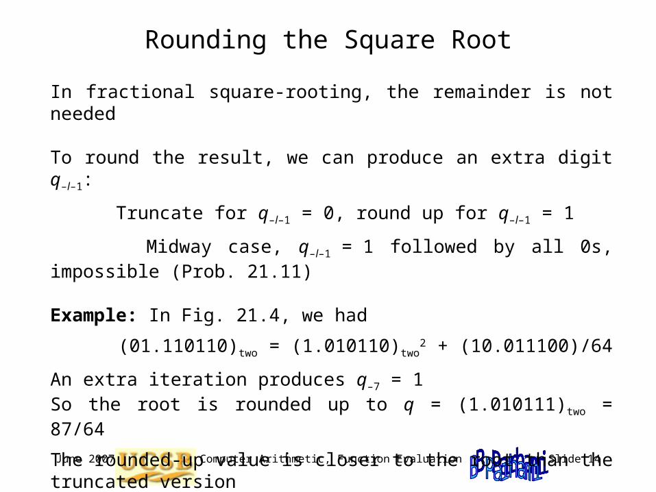
In fractional square-rooting, the remainder is not needed

To round the result, we can produce an extra digit q–l–1:

Truncate for q–l–1 = 0, round up for q–l–1 = 1

Midway case, q–l–1 = 1 followed by all 0s, impossible (Prob. 21.11)

Example: In Fig. 21.4, we had

(01.110110)two = (1.010110)two2 + (10.011100)/64

An extra iteration produces q–7 = 1 So the root is rounded up to q = (1.010111)two = 87/64

The rounded-up value is closer to the root than the truncated version

Original: 118/64 = (86/64)2 + 156/(64)2

Rounded: 118/64 = (87/64)2 – 17/(64)2


21.3 Binary Nonrestoring Algorithm

As in nonrestoring division, nonrestoring square-rooting implies:

Root digits in {1, 1} On-the-fly conversion to binary Possible final correction

The case q–j = 1 (nonnegative partial remainder), is handled as in the restoring algorithm; i.e., it leads to the trial subtraction of

q–j [2q (j–1) + 2–j

q–j ] = 2q (j–1) + 2–j

For q–j = 1, we must subtract

q–j [2q (j–1) + 2–j

q–j ] = – [2q (j–1) – 2–j

]

which is equivalent to adding 2q (j–1) – 2–j

Slight complication, compared with nonrestoring division

This term cannot be formed by concatenation


Finding the Sq. Root of z = 1.110110

via the Nonrestoring

Algorithm

================================z (radicand = 118/64) 0 1 . 1 1 0 1 1 0 ================================s(0) = z – 1 0 0 0 . 1 1 0 1 1 0 q0 = 1 1.2s(0) 0 0 1 . 1 0 1 1 0 0 q–1 = 1 1.1 –[2 1.)+2–1] 1 0 . 1 –––––––––––––––––––––––––––––––––s(1) 1 1 1 . 0 0 1 1 0 0 q–2 = 1 1.012s(1) 1 1 0 . 0 1 1 0 0 0 +[2 1.1)2–2] 1 0 . 1 1 –––––––––––––––––––––––––––––––––s(2) 0 0 1 . 0 0 1 0 0 0 q–3 = 1 1.0112s(2) 0 1 0 . 0 1 0 0 0 0–[2 1.01)+2–3] 1 0 . 1 0 1 –––––––––––––––––––––––––––––––––s(3) 1 1 1 . 1 0 1 0 0 0 q–4 = 1 1.01012s(3) 1 1 1 . 0 1 0 0 0 0+[2 1.011)2–4] 1 0 . 1 0 1 1 –––––––––––––––––––––––––––––––––s(4) 0 0 1 . 1 1 1 1 0 0 q–5 = 1 1.01011 2s(4) 0 1 1 . 1 1 1 0 0 0–[2 1.0101)+2–5] 1 0 . 1 0 1 0 1 –––––––––––––––––––––––––––––––––s(5) 0 0 1 . 0 0 1 1 1 0 q–6 = 1 1.0101112s(5) 0 1 0 . 0 1 1 1 0 0–[21.01011)+2–6] 1 0 . 1 0 1 1 0 1 –––––––––––––––––––––––––––––––––s(6) 1 1 1 . 1 0 1 1 1 1 Negative; (17/64)+[21.01011)2–6] 1 0 . 1 0 1 1 0 1 Correct–––––––––––––––––––––––––––––––––s(6) Corrected 0 1 0 . 0 1 1 1 0 0 (156/64)

s (remainder = 156/64) 0 . 0 0 0 0 1 0 0 1 1 1 0 0 (156/642)q (binary) 1 . 0 1 0 1 1 1 (87/64)q (corrected binary) 1 . 0 1 0 1 1 0 (86/64)================================

Fig. 21.6 Example of nonrestoring binary square-rooting.

Root digit

Partial root


Some Details for Nonrestoring Square-Rooting

Solution: We keep q (j–1) and q

(j–1) – 2–j+1 in registers Q (partial root) and Q* (diminished partial root), respectively. Then:

q–j = 1 Subtract 2q (j–1) + 2–j formed by shifting Q 01

q–j = 1 Add 2q (j–1) – 2–j formed by shifting Q*11

Updating rules for Q and Q* registers:

q–j = 1 Q := Q 1 Q* := Q 0 q–j = 1 Q := Q*1 Q* := Q*0

Depending on the sign of the partial remainder, add:

(positive) Add 2q (j–1) + 2–j

(negative) Sub. 2q (j–1) – 2–j

Cannot be formed by concatenationConcatenate 01 to the end of q

(j–1)

Additional rule for SRT-like algorithm that allow q–j = 0 as well:

q–j = 0 Q := Q 0 Q* := Q*1


2

0

3

Radicand


z

s Remainder

Root q

q 2 6 – q 2 4 – q 2 2

1 – q (q 2 0 –

(q (q (q

(1)

(0)

(2)

(3)

0 0 0 0

2

0

3 q q q 1 q

) ) ) )

21.4 High-Radix Square-Rooting

Basic recurrence for fractional radix-r square-rooting:

s (j) = rs

(j–1) – q–j(2 q (j–1) + r –j

q–j)

As in radix-2 nonrestoring algorithm, we can use two registers Q and Q* to hold q

(j–1) and its diminished version q (j–1) – r –j+1,

respectively, suitably updating them in each step

Radix-4 square-rooting in dot notationFig. 21.3


An Implementation of Radix-4 Square-Rooting

r = 4, root digit set [–2, 2]

Q* holds q (j–1) – 4–j+1 = q

(j–1) – 2–2j+2. Then, one of the following values must be subtracted from, or added to, the shifted partial remainder rs

(j–1)

q–j = 2 Subtract 4q (j–1) + 2–2j+2 double-shift Q 010

q–j = 1 Subtract 2q (j–1) + 2–2j shift Q 001

q–j = 1 Add 2q (j–1) – 2–2j shift Q*111

q–j = 2 Add 4q (j–1) – 2–2j+2 double-shift Q*110

Updating rules for Q and Q* registers:

q–j = 2 Q := Q 10 Q* := Q 01 q–j = 1 Q := Q 01 Q* := Q 00 q–j = 0 Q := Q 00 Q* := Q*11 q–j = 1 Q := Q*11 Q* := Q*10 q–j = 2 Q := Q*10 Q* := Q*01

Note that the root is obtained in binary form (no conversion needed!)

s (j) = rs

(j–1) – q–j(2 q (j–1) + r –j

q–j)


Keeping the Partial Remainder in Carry-Save Form

To keep magnitudes of partial remainders for division and square-rooting comparable, we can perform radix-4 square-rooting using the digit set

{1, ½ , 0 , ½ , 1}

Can convert from the digit set above to the digit set [–2, 2], or directly to binary, with no extra computation

Division: s (j) = 4s

(j–1) – q–j d

Square-rooting: s (j) = 4s

(j–1) – q–j (2 q (j–1) + 4 –j

q–j)

As in fast division, root digit selection can be based on a few bits of the shifted partial remainder 4s

(j–1) and of the partial root q (j–1)

This would allow us to keep s in carry-save formOne extra bit of each component of s (sum and carry) must be examined

Can use the same lookup table for quotient digit and root digit selectionTo see how, compare recurrences for radix-4 division and square-rooting:


21.5 Square-Rooting by Convergence

x

f(x)

z

z

Newton-Raphson method

Choose f(x) = x2 – z with a root at x = z

x (i+1) = x

(i) – f(x (i)) / f (x

(i))

x (i+1) = 0.5(x

(i) + z / x (i))

Each iteration: division, addition, 1-bit shiftConvergence is quadratic

For 0.5 z < 1, a good starting approximation is (1 + z)/2

This approximation needs no arithmetic

The error is 0 at z = 1 and has a max of 6.07% at z = 0.5

The hardware approximation method of Schwarz and Flynn, using the tree circuit of a fast multiplier, can provide a much better approximation (e.g., to 16 bits, needing only two iterations for 64 bits of precision)


Initial Approximation Using Table Lookup

Table-lookup can yield a better starting estimate x (0) for z

For example, with an initial estimate accurate to within 2–8, three iterations suffice to increase the accuracy of the root to 64 bits

x (i+1) = 0.5(x

(i) + z / x (i))

Example 21.1: Compute the square root of z = (2.4)ten

x (0) read out from table = 1.5 accurate to 10–1

x (1) = 0.5(x

(0) + 2.4 / x (0)) = 1.550 000 000 accurate to 10–2

x (2) = 0.5(x

(1) + 2.4 / x (1)) = 1.549 193 548 accurate to 10–4

x (3) = 0.5(x

(2) + 2.4 / x (2)) = 1.549 193 338 accurate to 10–8

Check: (1.549 193 338)2 = 2.399 999 999


Convergence Square-Rooting without Division

Rewrite the square-root recurrence as:

x (i+1) = x

(i) + 0.5 (1/x (i))(z – (x

(i))2) = x (i) + 0.5(x

(i))(z – (x (i))2)

where (x (i)) is an approximation to 1/x

(i) obtained by a simple circuit or read out from a table

Because of the approximation used in lieu of the exact value of 1/x (i),

convergence rate will be less than quadratic

Alternative: Use the recurrence above, but find the reciprocal iteratively; thus interlacing the two computations

Using the function f(y) = 1/y – x to compute 1/x, we get:

x (i+1) = 0.5(x

(i) + z y (i))

y (i+1) = y

(i) (2 – x

(i) y

(i))

Convergence is less than quadratic but better than linear

3 multiplications, 2 additions, and a 1-bit shift per iteration

x (i+1) = 0.5(x

(i) + z / x (i))


Example for Division-Free Square-Rooting

Example 21.2: Compute 1.4, beginning with x (0) = y

(0) = 1

x (1) = 0.5(x

(0) + 1.4 y (0)) = 1.200 000 000

y (1) = y

(0) (2 – x (0) y

(0)) = 1.000 000 000 x

(2) = 0.5(x (1) + 1.4 y

(1)) = 1.300 000 000 y

(2) = y (1) (2 – x

(1) y (1)) = 0.800 000 000

x (3) = 0.5(x

(2) + 1.4 y (2)) = 1.210 000 000

y (3) = y

(2) (2 – x (2) y

(2)) = 0.768 000 000 x

(4) = 0.5(x (3) + 1.4 y

(3)) = 1.142 600 000 y

(4) = y (3) (2 – x

(3) y (3)) = 0.822 312 960

x (5) = 0.5(x

(4) + 1.4 y (4)) = 1.146 919 072

y (5) = y

(4) (2 – x (4) y

(4)) = 0.872 001 394 x

(6) = 0.5(x (5) + 1.4 y

(5)) = 1.183 860 512 1.4

x (i+1) = 0.5(x

(i) + z y (i))

y (i+1) = y

(i) (2 – x

(i) y

(i))x converges to zy converges to 1/z

Check: (1.183 860 512)2 = 1.401 525 712


Another Division-Free Convergence Scheme

Based on computing 1/z, which is then multiplied by z to obtain z The function f(x) = 1/x2 – z has a root at x = 1/z (f (x) = –2/x3)

x (i+1) = 0.5 x

(i) (3 – z (x

(i))2)

Quadratic convergence

3 multiplications, 1 addition, and a 1-bit shift per iteration

Cray 2 supercomputer used this method. Initially, instead of x (0), the

two values 1.5 x (0) and 0.5(x

(0))3 are read out from a table, requiring only 1 multiplication in the first iteration. The value x

(1) thus obtained is accurate to within half the machine precision, so only one other iteration is needed (in all, 5 multiplications, 2 additions, 2 shifts)

Example 21.3: Compute the square root of z = (.5678)ten

x (0) read out from table = 1.3

x (1) = 0.5x

(0) (3 – 0.5678 (x

(0))2) = 1.326 271 700 x

(2) = 0.5x (1)

(3 – 0.5678 (x (1))2) = 1.327 095 128

z z x (2) = 0.753 524 613


2

0

3

Radicand


z

s Remainder

Root q

q 2 6 – q 2 4 – q 2 2

1 – q (q 2 0 –

(q (q (q

(1)

(0)

(2)

(3)

0 0 0 0

2

0

3 q q q 1 q

) ) ) )

21.6 Parallel Hardware Square-Rooters

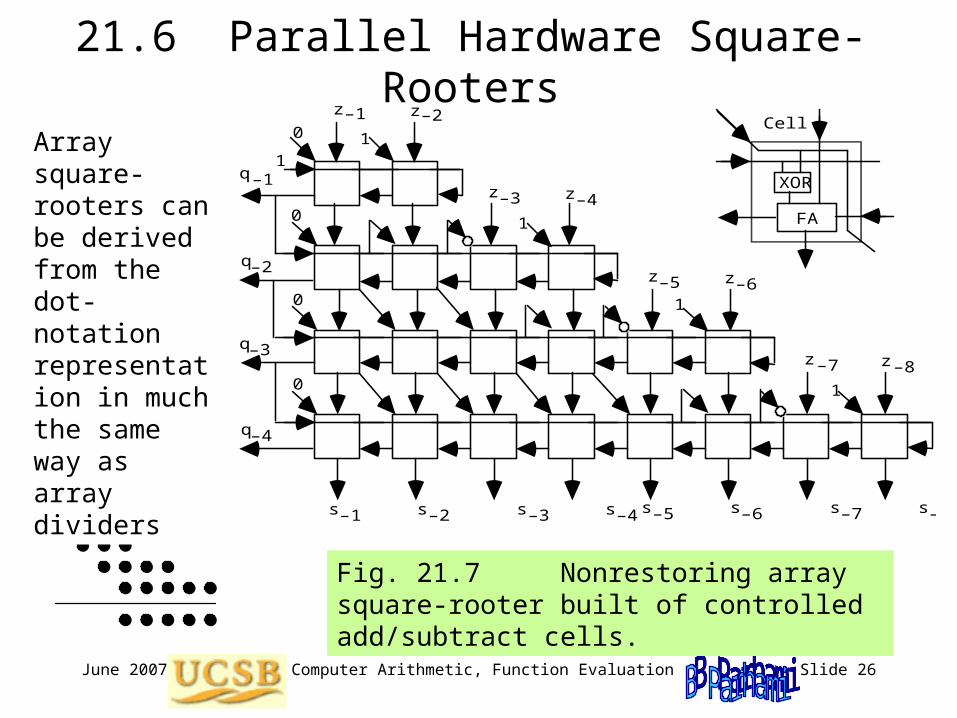
Array square-rooters can be derived from the dot-notation representation in much the same way as array dividers

Fig. 21.7 Nonrestoring array square-rooter built of controlled add/subtract cells.

Radicand z = .z z z z z z z z Root q = .q q q q Remainder s = .s s s s s s s s

–1 –2 –3 –4 –5 –6 –7 –8 –1 –2 –3 –4 –1 –2 –3 –4 –5 –6 –7 –8

s s s s–1 –2 –3 –4

q

q

–1

–2

q–3

FA

XOR

Cell

s s s s–5 –6 –7 –8

q–4

z z–1 –2

z z–3 –4

z z–5 –6

z z–7 –8

1

1

1

10

0

0

0

1


Understanding the Array Square-Rooter Design

Description goes hereRadicand z = .z z z z z z z z Root q = .q q q q Remainder s = .s s s s s s s s

–1 –2 –3 –4 –5 –6 –7 –8 –1 –2 –3 –4 –1 –2 –3 –4 –5 –6 –7 –8

s s s s–1 –2 –3 –4

q

q

–1

–2

q–3

FA

XOR

Cell

s s s s–5 –6 –7 –8

q–4

z z–1 –2

z z–3 –4

z z–5 –6

z z–7 –8

1

1

1

10

0

0

0

1


Nonrestoring Array Square-Rooter in Action

Check: 118/256 = (10/16)2 + (3/256)? Note that the answer is approximate (to within 1 ulp) due to there being no final correction

0 1 0

Radicand z = .z z z z z z z z Root q = .q q q q Remainder s = .s s s s s s s s

–1 –2 –3 –4 –5 –6 –7 –8 –1 –2 –3 –4 –1 –2 –3 –4 –5 –6 –7 –8

s s s s–1 –2 –3 –4

q

q

–1

–2

q–3

FA

XOR

Cell

s s s s–5 –6 –7 –8

q–4

z z–1 –2

z z–3 –4

z z–5 –6

z z–7 –8

1

1

1

10

0

0

0

1

0 1

1 1

0 1

1

1

0

1

0

0 0

0 1

0 1 0 1

1 1 1 0

0 0 1 0 1 1

0 0 0 1 0 0

0 0 0 1 0 1 0 1

1 1 1 1 1 1 0 1

1

1

0

1

1

110

11011

0100000

0


Root digit

Partial root

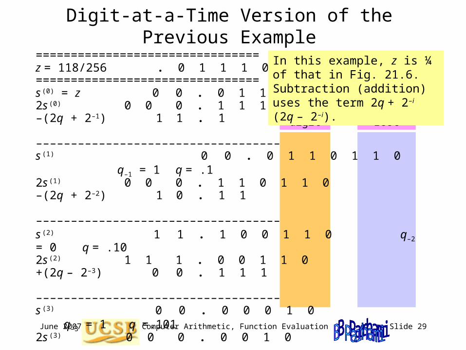
Digit-at-a-Time Version of the Previous Example

================================z = 118/256 . 0 1 1 1 0 1 1 0 ================================s

(0) = z 0 0 . 0 1 1 1 0 1 1 0 2s

(0) 0 0 0 . 1 1 1 0 1 1 0 –(2q + 2–1) 1 1 . 1 –––––––––––––––––––––––––––––––––––s

(1) 0 0 . 0 1 1 0 1 1 0 q–1 = 1 q = .1 2s

(1) 0 0 0 . 1 1 0 1 1 0 –(2q + 2–2) 1 0 . 1 1 –––––––––––––––––––––––––––––––––––s

(2) 1 1 . 1 0 0 1 1 0 q–2 = 0 q = .10 2s

(2) 1 1 1 . 0 0 1 1 0 +(2q – 2–3) 0 0 . 1 1 1 –––––––––––––––––––––––––––––––––––s

(3) 0 0 . 0 0 0 1 0 q–3 = 1 q =.1012s

(3) 0 0 0 . 0 0 1 0 –(2q + 2–4) 1 0 . 1 0 1 1 –––––––––––––––––––––––––––––––––––s

(4) 1 0 . 1 1 0 1 q–4 = 0 q = .1010=================================

In this example, z is ¼ of that in Fig. 21.6. Subtraction (addition) uses the term 2q + 2–i (2q – 2–i).


22 The CORDIC Algorithms

Chapter Goals

Learning a useful convergence method for evaluating trigonometric and other functions

Chapter Highlights

Basic CORDIC idea: rotate a vector with end point at (x,y) = (1,0) by the angle z to put its end point at (cos z, sin z)Other functions evaluated similarlyComplexity comparable to division


The CORDIC Algorithms: Topics


22.1. Rotations and Pseudorotations

22.2. Basic CORDIC Iterations

22.3. CORDIC Hardware

22.4. Generalized CORDIC

22.5. Using the CORDIC Method

22.6. An Algebraic Formulation


22.1 Rotations and Pseudorotations

-

If we have a computationally efficient way of rotating a vector, we can evaluate cos, sin, and tan–1 functions

Rotation by an arbitrary angle is difficult, so we:

Perform psuedorotations that require simpler operations Use special angles to synthesize the desired angle z

z = (1) +

(2) + . . . + (m)

Key ideas in CORDIC

COordinate Rotation DIgital Computer used this method in 1950s; modern electronic calculators also use it

z

(cos z, sin z)

(1, 0)

tan y

(1, y)

–1

start at (1, 0) rotate by z get cos z, sin z

start at (1, y) rotate until y = 0 rotation amount is tan y –1


Rotating a Vector (x (i), y

(i)) by the Angle (i)

Fig. 22.1 A pseudorotation step in CORDIC

x

y Rotation

Pseudo- rotation

O

R (i+1)

R (i) (i)

E (i+1) E (i+1)

E (i)

y (i+1)

x (i+1)

y (i)

x (i)

Our strategy: Eliminate the terms (1 + tan2

(i))1/2 and choose the angles (i)) so that tan (i) is a power of 2; need two shift-adds

x(i+1) = x(i) cos (i) – y(i) sin (i) = (x(i) – y(i) tan (i)) / (1 + tan2 (i))1/2

y(i+1) = y(i) cos (i) + x(i) sin (i) = (y(i) + x(i) tan (i)) / (1 + tan2 (i))1/2

z(i+1) = z(i) – (i) Recall that cos = 1 / (1 + tan2 )1/2


Pseudorotating a Vector (x (i), y

(i)) by the Angle (i)

Fig. 22.1 A pseudorotation step in CORDIC

x

y Rotation

Pseudo- rotation

O

R (i+1)

R (i) (i)

E (i+1) E (i+1)

E (i)

y (i+1)

x (i+1)

y (i)

x (i)

Pseudorotation: Whereas a real rotation does not change the length R(i) of the vector, a pseudorotation step increases its length to:

R(i+1) = R(i) / cos (i) = R(i) (1 + tan2

(i))1/2

x(i+1) = x(i) – y(i) tan (i)

y(i+1) = y(i) + x(i) tan (i)

z(i+1) = z(i) – (i)


A Sequence of Rotations or Pseudorotations

After m real rotations by (1), (2) , . . . , (m) , given x(0) = x, y(0) = y, and z(0) = z

x(m) = x cos((i)) – y sin((i))

x(m) = y cos((i)) + x sin((i))

z(m) = z – ((i))

x(m) = K(x cos((i)) – y sin((i)))

y(m) = K(y cos((i)) + x sin((i)))

z(m) = z – ((i))

where K = (1 + tan2 (i))1/2 is

a constant if angles of rotation are always the same, differing only in sign or direction

After m pseudorotations by (1), (2) , . . . , (m) , given x(0) = x, y(0) = y, and z(0) = z

(1)

(2)

(3)

Question: Can we find a set of angles so that any angle can be synthesized from all of them with appropriate signs?


22.2 Basic CORDIC Iterations

CORDIC iteration: In step i, we pseudorotate by an angle whose tangent is di 2–i (the angle

e(i) is fixed, only direction di is to be picked)

x(i+1) = x(i) – di y(i) 2–i

y(i+1) = y(i) + di x(i) 2–i

z(i+1) = z(i) – di tan –1 2–i

= z(i) – di e(i) –––––––––––––––––––––––––––––––– i –––––––––––––––––––––––––––––––– 0 45.0 0.785 398 163 1 26.6 0.463 647 609 2 14.0 0.244 978 663 3 7.1 0.124 354 994 4 3.6 0.062 418 810 5 1.8 0.031 239 833 6 0.9 0.015 623 728 7 0.4 0.007 812 341 8 0.2 0.003 906 230 9 0.1 0.001 953 123––––––––––––––––––––––––––––––––

e(i) in degrees(approximate)

e(i) in radians(precise)

Table 22.1 Value of the function e(i) = tan

–1 2–i,in degrees and radians, for 0 i 9

Example: 30 angle

30.0 45.0 – 26.6 + 14.0 – 7.1 + 3.6 + 1.8 – 0.9 + 0.4 – 0.2 + 0.1 = 30.1


Choosing the Angles to Force z to Zero

x(i+1) = x(i) – di y(i) 2–i

y(i+1) = y(i) + di x(i) 2–i

z(i+1) = z(i) – di tan –1 2–i

= z(i) – di e(i) ––––––––––––––––––––––––––––––– i z(i) – di e(i) = z(i+1) ––––––––––––––––––––––––––––––– +30.0 0 +30.0 – 45.0 = –15.0 1 –15.0 + 26.6 = +11.6 2 +11.6 – 14.0 = –2.4 3 –2.4 + 7.1 = +4.7 4 +4.7 – 3.6 = +1.1 5 +1.1 – 1.8 = –0.7 6 –0.7 + 0.9 = +0.2 7 +0.2 – 0.4 = –0.2 8 –0.2 + 0.2 = +0.0 9 +0.0 – 0.1 = –0.1–––––––––––––––––––––––––––––––

Table 22.2 Choosing the signs of the rotation angles in order to force z to 0

y

x

x ,y

x–45

+26.6

–1430

(0) (0)

(10)

x ,y(1) (1)

x ,y(2) (2)

x ,y(3) (3)

Fig. 22.2 The first three of 10 pseudorotations leading from (x(0), y(0)) to (x(10), 0) in rotating by +30.


Why Any Angle Can Be Formed from Our List

Analogy: Paying a certain amount while using all currency denominations (in positive or negative direction) exactly once; red values are fictitious.

$20 $10 $5 $3 $2 $1 $.50 $.25 $.20 $.10 $.05 $.03 $.02 $.01

Example: Pay $12.50

$20 – $10 + $5 – $3 + $2 – $1 – $.50 + $.25 – $.20 – $.10 + $.05 + $.03 – $.02 – $.01

Convergence is possible as long as each denomination is no greater than the sum of all denominations that follow it.

Domain of convergence: –$42.16 to +$42.16

We can guarantee convergence with actual denominations if we allow multiple steps at some values:

$20 $10 $5 $2 $2 $1 $.50 $.25 $.10 $.10 $.05 $.01 $.01 $.01 $.01

Example: Pay $12.50

$20 – $10 + $5 – $2 – $2 + $1 + $.50+$.25–$.10–$.10–$.05+$.01–$.01+ $.01–$.01

We will see later that in hyperbolic CORDIC, convergence is guaranteed only if certain “angles” are used twice.


Using CORDIC in Rotation Mode

x(i+1) = x(i) – di y(i) 2–i

y(i+1) = y(i) + di x(i) 2–i

z(i+1) = z(i) – di tan –1 2–i

= z(i) – di e(i)

For k bits of precision in results, k CORDIC iterations are needed, because tan

–1 2–i 2–I for large i

x(m) = K(x cos z – y sin z)

y(m) = K(y cos z + x sin z)

z(m) = 0

where K = 1.646 760 258 121 . . .

Make z converge to 0 by choosing di = sign(z(i))

0

0

Start with

x = 1/K = 0.607 252 935 . . .

and y = 0

to find cos z and sin z

Convergence of z to 0 is possible because each of the angles in our list is more than half the previous one or, equivalently, each is less than the sum of all the angles that follow it

Domain of convergence is –99.7˚ ≤ z ≤ 99.7˚, where 99.7˚ is the sum of all the angles in our list; the domain contains [–/2, /2] radians


Using CORDIC in Vectoring Mode

x(i+1) = x(i) – di y(i) 2–i

y(i+1) = y(i) + di x(i) 2–i

z(i+1) = z(i) – di tan –1 2–i

= z(i) – di e(i)

For k bits of precision in results, k CORDIC iterations are needed, because tan

–1 2–i 2–I for large i

x(m) = K(x2 + y2)1/2

y(m) = 0

z(m) = z + tan –1(y / x)

where K = 1.646 760 258 121 . . .

Make y converge to 0 by choosing di = – sign(x(i)y(i))

0

Start with

x = 1 and z = 0

to find tan –1

y

Even though the computation above always converges, one can use the relationship tan

–1(1/y ) = /2 – tan –1y

to limit the range of fixed-point numbers encountered

Other trig functions: tan z obtained from sin z and cos z via division;inverse sine and cosine (sin

–1 z and cos

–1 z) discussed later


22.3 CORDIC Hardware

x

y

z

Shift

Shift

±

±

±

Lookup Table

Fig. 22.3 Hardware elements needed for the CORDIC method.

x(i+1) = x(i) – di y(i) 2–i

y(i+1) = y(i) + di x(i) 2–i

z(i+1) = z(i) – di tan –1 2–i

= z(i) – di e(i) If very high speed is not needed (as in a calculator), a single adder and one shifter would suffice

k table entries for k bits of precision


22.4 Generalized CORDIC

Fig. 22.4 Circular, linear, and hyperbolic CORDIC.

x

y

O

B A

F

E

C

D

= –1 = 1 = 0

U V W

x(i+1) = x(i) – di y(i) 2–i

y(i+1) = y(i) + di x(i) 2–i

z(i+1) = z(i) – di e(i)

= 1 Circular rotations (basic CORDIC)

e(i) = tan –1 2–i

= 0 Linear rotationse(i) = 2–i

= –1 Hyperbolic rotationse(i) = tanh

–1 2–i


22.5 Using the CORDIC Method

Fig. 22.5 Summary of generalized CORDIC algorithms.

For cos & sin, set x = 1/K, y = 0

tan z = sin z / cos z

For tan , set x = 1, z = 0

–1

For multiplication, set y = 0

For division, set z = 0

In executing the iterations for = –1, steps 4, 13, 40, 121, . . . , j , 3j + 1, . . .

must be repeated. These repetitions are incorporated in the constant K' below.

For cosh & sinh, set x = 1/K', y = 0

tanh z = sinh z / cosh z exp(z) = sinh z + cosh z

For tanh , set x = 1, z = 0

–1

w = exp(t ln w)

t

ln w = 2 tanh |(w – 1)/(w + 1)|

–1

Rotation: d = sign(z ),

i

z 0

(i)

(i)

e =

= 1 Circular

tan 2

–i

(i) –1

= –1 Hyperbolic

e =

(i)

tanh 2

–i

–1

Mode Vectoring: d = –sign(x y ),

i

(i)

(i)

y 0

(i)

K(x cos z – y sin z) K(y cos z + x sin z) 0

x y z

C O R D I C

x y + xz 0

x y z

C O R D I C

x 0

z + y/x

x y z

C O R D I C

K' (x cosh z – y sinh z) K' (y cosh z + x sinh z) 0

x y z

C O R D I C

0 z + tan (y/x)

–1

x y z

C O R D I C

K x + y

2

2

0 z + tanh (y/x)

–1

x y z

C O R D I C

K' x – y

2

2

cos w = tan [1 – w / w]

2

–1

–1

sin w = tan [w / 1 – w ]

2

–1

–1

w = (w + 1/4) – (w – 1/4)

2

2

cosh w = ln(w + 1 – w )

–1

2

sinh w = ln(w + 1 + w )

–1

2

Note

e = 2

= 0 Linear

(i)

–i

x(i+1) = x(i) – di y(i) 2–i

y(i+1) = y(i) + di x(i) 2–i

z(i+1) = z(i) – di e(i) {–1, 0, 1} di {–1, 1} K = 1.646 760 258 121 ...1/K = .607 252 935 009 ...K' = .828 159 360 960 2 ...1/K' = 1.207 497 067 763 ...


CORDIC Speedup Methods

x(i+1) = x(i) – di y(i) 2–i

y(i+1) = y(i) + di x(i) 2–i

z(i+1) = z(i) – di e(i)

Skipping some rotationsMust keep track of expansion via the recurrence:

(K(i+1))2 = (K(i))2 (1 ± 2–2i)

This additional work makes variable-factor CORDIC less cost-effective than constant-factor CORDIC

Early terminationDo the first k/2 iterations as usual, then combine the remaining k/2 into a single multiplicative step:

For very small z, we have tan–1 z z tan z

Expansion factor not an issue because contribution of the ignored terms is provably less than ulp

x(k) = x(k/2) – y(k/2) z(k/2)

y(k) = y(i) + x(k/2) z(k/2)

z(k) = z(k/2) – z(k/2)

High-radix CORDICThe hardware for the radix-4 version of CORDIC is quite similar to Fig. 22.3

di {–2, –1, 1, 2} or

{–2, –1, 0, 1, 2}


22.6 An Algebraic Formulation

Because

cos z + j sin z = e jz where j = –1

cos z and sin z can be computed via evaluating the complex exponential function e

jz

This leads to an alternate derivation of CORDIC iterations

Details in the text


23 Variations in Function Evaluation

Chapter Goals

Learning alternate computation methods (convergence and otherwise) for somefunctions computable through CORDIC

Chapter Highlights

Reasons for needing alternate methods: Achieve higher performance or precision Allow speed/cost tradeoffsOptimizations, fit to diverse technologies


Variations in Function Evaluation: Topics


23.1. Additive / Multiplicative Normalization

23.2. Computing Logarithms

23.3. Exponentiation

23.4. Division and Square-Rooting, Again

23.5. Use of Approximating Functions

23.6. Merged Arithmetic


23.1 Additive / Multiplicative Normalization

u (i+1) = f(u

(i), v (i), w

(i))

v (i+1) = g(u

(i), v (i), w

(i))

w (i+1) = h(u

(i), v (i), w

(i))

u (i+1) = f(u

(i), v (i))

v (i+1) = g(u

(i), v (i))

Additive normalization: Normalize u via addition of terms to it

Constant

Desiredfunction

Guide the iteration such that one of the values converges to a constant (usually 0 or 1); this is known as normalization

The other value then converges to the desired function

Multiplicative normalization: Normalize u via multiplication of terms

Additive normalization is more desirable, unless the multiplicative terms are of the form 1 ± 2a (shift-add) or multiplication leads to much faster convergence compared with addition


Convergence Methods You Already Know

CORDICExample of additive normalization x(i+1) = x(i) – di y(i)

2–i

y(i+1) = y(i) + di x(i) 2–i

z(i+1) = z(i) – di e(i)

Division by repeated multiplicationsExample of multiplicative normalization

d (i+1) = d

(i) (2 d

(i)) Set d (0) = d; iterate until d

(m) 1

z (i+1) = z

(i) (2 d

(i)) Set z (0) = z; obtain z/d = q z

(m)

Force y or z to 0 byadding terms to it

Force d to 1 bymultiplying terms with it


23.2 Computing Logarithms

x (i+1) = x

(i) c

(i) = x (i)

(1 + di 2–i)

y (i+1) = y

(i) – ln c (i) = y

(i) – ln(1 + di 2–i)

Read out from table

Force x (m) to 1

y (m) converges to y + ln x

di {1, 0, 1}

0

Why does this multiplicative normalization method work?

x (m) = x c

(i) 1 c

(i) 1/x

y (m) = y – ln c

(i) = y – ln (c (i)) = y – ln(1/x) y + ln x

Convergence domain: 1/(1 + 2–i) x 1/(1 – 2–i) or 0.21 x 3.45

Number of iterations: k, for k bits of precision; for large i, ln(1 2–i) 2–i

Use directly for x [1, 2). For x = 2q s, we have:ln x = q ln 2 + ln s = 0.693 147 180 q + ln s

Radix-4 version can be devised


Computing Binary Logarithms via Squaring

log x

Squarer

Initialized to x

value 2 iff this bit is 1

2

Radix Shift 0 1

Point Fig. 23.1 Hardware elements needed for computing log2 x.

For x [1, 2), log2 x is a fractional number y = (. y–1y–2y–3 . . . y–l)two

x = 2y = 2

x 2 = 22y = 2 y–1 = 1 iff x

2 2

(. y–1y–2y–3 . . . y–l)two

(y–1. y–2y–3 . . . y–l)two

Once y–1 has been determined, if y–1 = 0, we are back at the original situation; otherwise, divide both sides of the equation above by 2 to get:

x 2/2 = 2 /2 = 2

(1 . y–2y–3 . . . y–l)two (. y–2y–3 . . . y–l)two

Generalization to base b:

x = b

y–1 = 1 iff x 2 b

(. y–1y–2y–3 . . . y–l)two


23.3 Exponentiation

x (i+1) = x

(i) – ln c

(i) = x (i)

– ln(1 + di 2–i)

y (i+1) = y

(i) c

(i) = y (i)

(1 + di 2–i)

Read out from table

Force x (m) to 0

y (m) converges to y ex

di {1, 0, 1}1

Why does this additive normalization method work?

x (m) = x – ln c

(i) 0 ln c (i)

x

y (m) = y c

(i) = y exp(ln c (i)) = y exp( ln c

(i)) y ex

Convergence domain: ln (1 – 2–i) x ln (1 + 2–i) or –1.24 x 1.56

Number of iterations: k, for k bits of precision; for large i, ln(1 2–i) 2–i

Can eliminate half the iterations becauseln(1 + ) = – 2/2 + 3/3 – . . . for 2 < ulpand we may write y

(k) = y

(k/2) (1 + x

(k/2))

Radix-4 version can be devised

Computing ex


General Exponentiation, or Computing xy

x y = (e

ln x) y

= e y ln x So, compute natural log, multiply, exponentiate

When y is an integer, we can exponentiate by repeated multiplication (need to consider only positive y; for negative y, compute reciprocal)

In particular, when y is a constant, the methods used are reminiscent of multiplication by constants (Section 9.5)

Example: x 25 = ((((x)2x)2)2)2x [4 squarings and 2 multiplications]

Noting that 25 = (1 1 0 0 1)two, leads to a general procedure

Computing x y, when y is an unsigned integer

Initialize the partial result to 1 Scan the binary representation of y, starting at its MSB, and repeat If the current bit is 1, multiply the partial result by x If the current bit is 0, do not change the partial result Square the partial result before the next step (if any)


Faster Exponentiation via Recoding

Radix-4 example: 31 = (1 1 1 1 1)two = (1 0 0 0 01)two = (2 0 1)four

x 31 = (((x2)4)4 / x [Can you formulate the general procedure?]

Example: x 31 = ((((x)2x)2x)2x)2x [4 squarings and 4 multiplications]

Note that 31 = (1 1 1 1 1)two = (1 0 0 0 01)two

x 31 = (((((x)2)2)2)2)2 / x [5 squarings and 1 division]

Computing x y, when y is an integer encoded in BSD format

Initialize the partial result to 1 Scan the binary representation of y, starting at its MSB, and repeat If the current digit is 1, multiply the partial result by x If the current digit is 0, do not change the partial result If the current digit is 1, divide the partial result by x Square the partial result before the next step (if any)


23.4 Division and Square-Rooting, Again

s (i+1) = s

(i) –

(i) d

q (i+1) = q

(i) + (i)

Computing q = z / d In digit-recurrence division, (i) is the next

quotient digit and the addition for q turns into concatenation; more generally,

(i) can be any estimate for the difference between the partial quotient q

(i) and the final quotient q

Because s (i)

becomes successively smaller as it converges to 0, scaled versions of the recurrences above are usually preferred. In the following, s

(i) stands for s

(i) r

i and q (i) for q

(i) r

i :

s (i+1) = rs

(i) –

(i) d Set s

(0) = z and keep s (i) bounded

q (i+1) = rq

(i) + (i)

Set q (0) = 0 and find q * = q

(m) r

–m

In the scaled version, (i)

is an estimate for r (r i–m

q – q (i)) = r (r

i q * - q

(i)), where q * = r

–m q represents the true quotient


Square-Rooting via Multiplicative Normalization

Idea: If z is multiplied by a sequence of values (c (i))2, chosen so that the

product z (c (i))2 converges to 1, then z c

(i) converges to z

x (i+1) = x

(i) (1 + di 2–i)2 = x

(i) (1 + 2di 2–i + di

2 2–2i) x

(0) = z, x

(m) 1

y (i+1) = y

(i) (1 + di 2–i) y

(0) = z, y

(m) z

What remains is to devise a scheme for choosing di values in {–1, 0, 1}

di = 1 for x (i)

< 1 – = 1 – 2–i di = –1 for x (i)

> 1 + = 1 + 2–i

To avoid the need for comparison with a different constant in each step, a scaled version of the first recurrence is used in which u

(i) = 2i (x (i) – 1):

u (i+1) = 2(u

(i) + 2di) + 2–i+1(2di u (i) + di

2) + 2–2i+1di2

u (i) u

(0) = z – 1, u

(m) 0

y (i+1) = y

(i) (1 + di 2–i) y

(0) = z, y

(m) z

Radix-4 version can be devised: Digit set [–2, 2] or {–1, –½, 0, ½, 1}


Square-Rooting via Additive Normalization

Idea: If a sequence of values c (i) can be obtained such that z – (c

(i))2 converges to 0, then c

(i) converges to z

x (i+1)

= z – (y (i+1))2 = z – (y

(i) + c

(i))2 = x (i)

+ 2di y (i)

2–i – di2

2–2i x

(0) = z, x

(m) 0

y (i+1) = y

(i) + c

(i) = y

(i) – di 2–i y

(0) = 0, y

(m) z

What remains is to devise a scheme for choosing di values in {–1, 0, 1}

di = 1 for x (i)

< – = – 2–i di = –1 for x (i)

> + = + 2–i

To avoid the need for comparison with a different constant in each step, a scaled version of the first recurrence may be used in which u

(i) = 2i x (i):

u (i+1) = 2(u

(i) + 2di y (i) – di

2 2–i

) u (0)

= z , u (i) bounded

y (i+1) = y

(i) – di 2–i y

(0) = 0, y

(m) z

Radix-4 version can be devised: Digit set [–2, 2] or {–1, –½, 0, ½, 1}


23.5 Use of Approximating Functions

Convert the problem of evaluating the function f to that of function g approximating f, perhaps with a few pre- and postprocessing operations

Approximating polynomials need only additions and multiplications

Polynomial approximations can be derived from various schemes

The Taylor-series expansion of f(x) about x = a is

f(x) = j=0 to f (j)

(a) (x – a) j / j!

The error due to omitting terms of degree > m is:

f (m+1)

(a + (x – a)) (x – a)m+1 / (m + 1)! 0 < < 1

Setting a = 0 yields the Maclaurin-series expansion

f(x) = j=0 to f (j)

(0) x j / j!

and its corresponding error bound:

f (m+1)

(x) xm+1 / (m + 1)! 0 < < 1

Efficiency in computation can be gained via Horner’s method and incremental evaluation


Some Polynomial Approximations (Table 23.1)–––––––––––––––––––––––––––––––––––––––––––––––––––––––––––Func Polynomial approximation Conditions–––––––––––––––––––––––––––––––––––––––––––––––––––––––––––

1/x 1 + y + y 2 + y

3 + . . . + y i + . . . 0 < x < 2, y = 1 – x

ex 1 + x /1! + x 2/2! + x

3/3! + . . . + x i /i ! + . . .

ln x –y – y 2/2 – y

3/3 – y 4/4 – . . . – y

i /i – . . . 0 < x 2, y = 1 – x

ln x 2 [z + z 3/3 + z

5/5 + . . . + z 2i+1/(2i + 1) + . . . ] x > 0, z =

x–1x+1

sin x x – x 3/3! + x

5/5! – x 7/7! +

. . . + (–1)i

x2i+1/(2i + 1)! + . . .

cos x 1 – x 2/2! + x

4/4! – x 6/6! +

. . . + (–1)i

x2i /(2i )! +

. . .

tan–1 x x – x

3/3 + x 5/5 – x

7/7 + . . .

+ (–1)i x2i+1/(2i + 1) +

. . . –1 < x < 1

sinh x x + x 3/3! + x

5/5! + x 7/7! +

. . . + x2i+1/(2i + 1)! +

. . .

cosh x 1 + x 2/2! + x

4/4! + x 6/6! +

. . . + x2i

/(2i )! + . . .

tanh–1x x + x 3/3 + x

5/5 + x 7/7 +

. . . + x2i+1/(2i + 1) +

. . . –1 < x < 1–––––––––––––––––––––––––––––––––––––––––––––––––––––––––––


Function Evaluation via Divide-and-Conquer

Let x in [0, 4) be the (l + 2)-bit significand of a floating-point number or its shifted version. Divide x into two chunks x H and x L:

x = x H + 2–t x L

0 x H < 4 t + 2 bits

0 x L < 1 l – t bits

t bits

x H in [0, 4) x L in [0, 1)

The Taylor-series expansion of f(x) about x = x H is

f(x) = j=0 to f (j)

(x H) (2–t x L)

j / j!

A linear approximation is obtained by taking only the first two terms

f(x) f (x H) + 2–t x L f (x H)

If t is not too large, f and/or f (and other derivatives of f, if needed) can be evaluated via table lookup


Approximation by the Ratio of Two Polynomials

Example, yielding good results for many elementary functions

f(x)

a(5)x5 + a(4)x4 + a(3)x3 + a(2)x2 + a(1)x + a(0)

b(5)x5 + b(4)x4 + b(3)x3 + b(2)x2 + b(1)x + b(0)

Using Horner’s method, such a “rational approximation” needs 10 multiplications, 10 additions, and 1 division


23.6 Merged ArithmeticOur methods thus far rely on word-level building-block operations such as addition, multiplication, shifting, . . .

Sometimes, we can compute a function of interest directly without breaking it down into conventional operations

Example: merged arithmetic for inner product computation

z = z (0) + x

(1) y

(1) + x (2)

y (2) + x

(3) y

(3)

x(1) y(1)

x(3) y(3)

x(2) y(2)

z(0)

Fig. 23.2 Merged-arithmetic computation of an inner product followed by accumulation.


Example of Merged Arithmetic Implementation

Example: Inner product computation

z = z (0) + x

(1) y

(1) + x (2)

y (2) + x

(3) y

(3)

x(1) y(1)

x(3) y(3)

x(2) y(2)

z(0)

Fig. 23.3 Tabular representation of the dot matrix for inner-product computation and its reduction.

1 4 7 10 13 10 7 4 16 FAs 2 4 6 8 8 6 4 2 10 FAs + 1 HA 3 4 4 6 6 3 3 1 9 FAs1 2 3 4 4 3 2 1 1 4 FAs + 1 HA1 3 2 3 3 2 1 1 1 3 FAs + 2 HAs2 2 2 2 2 1 1 1 1 5-bit CPA

Fig. 23.2


Another Merged Arithmetic Example

Approximation of reciprocal (1/x) and reciprocal square root (1/x) functions with 29-30 bits of precision, so that a long floating-point result can be obtained with just one iteration at the end [Pine02]

u v w 1.

c Table

b Table

a Table

Squarer Radix-4 Booth

Radix-4 Booth

Partial products gen Partial products gen

9 bits 24 bits 19 bits

30 bits 20 bits 12 bits

16 bits

Multioperand adder

30 bits, carry-save

Double-precision significand f(x) = c + bv + av

2

1 square

Comparable to a multiplier

2 mult’s

2 adds


24 Arithmetic by Table Lookup

Chapter Goals

Learning table lookup techniquesfor flexible and dense VLSI realizationof arithmetic functions

Chapter Highlights

We have used tables to simplify or speedupq digit selection, convergence methods, . . . Now come tables as primary computationalmechanisms (as stars, not supporting cast)


Arithmetic by Table Lookup: Topics


24.1. Direct and Indirect Table Lookup

24.2. Binary-to-Unary Reduction

24.3. Tables in Bit-Serial Arithmetic

24.4. Interpolating Memory

24.5. Tradeoffs in Cost, Speed, and Accuracy

24.6. Piecewise Lookup Tables


24.1 Direct and Indirect Table Lookup

2 by table

Result(s) bits

Pre- processing logic

Post- processing logic

Smaller table(s)

Operand(s) bitsu u v

v

Operand(s) bitsu

Result(s) bitsv

.

.

.

. . .

Fig. 24.1 Direct table lookup versus table-lookup with pre- and post-processing.


Tables in Supporting and Primary Roles

Tables are used in two ways:

In supporting role, as in initial estimate for division

As main computing mechanism

Boundary between two uses is fuzzy

Pure logic Hybrid solutions Pure tabular

Previously, we started with the goal of designing logic circuits for particular arithmetic computations and ended up using tables to facilitate or speed up certain steps

Here, we aim for a tabular implementation and end up using peripheral logic circuits to reduce the table size

Some solutions can be derived starting at either endpoint


Lx + +() Lx + ()

24.2 Binary-to-Unary Reduction

Strategy: Reduce the table size by using an auxiliary unary function to evaluate a desired binary function Example 1: Addition/subtraction in a logarithmic number system; i.e., finding Lz = log(x y), given Lx and Ly

Solution: Let = Ly – Lx

Lz = log(x y)

= log(x (1 y/x))

= log x + log(1 y/x)

= Lx + log(1 log –1)

Pre-process

+ table table

Post-process

Lx

Ly

Lz

= Ly – Lx


Another Example of Binary-to-Unary ReductionExample 2: Multiplication via squaring, xy = (x + y)2/4 – (x – y)2/4

Simplification and implementation details

If x and y are k bits wide,x + y and x – y are k + 1bits wide, leading to twotables of size 2k+1

2k(total table size = 2k+3

k bits)

(x y)/2 = (x y)/2 + /2 {0, 1} is the LSB

(x + y)2/4 – (x – y)2/4 = [ (x + y)/2 + /2]

2 – [ (x – y)/2 + /2] 2

= (x + y)/2 2 – (x – y)/2

2 + y

Pre-process: compute x + y and x – y; drop their LSBsTable lookup: consult two squaring table(s) of size 2k

(2k – 1)Post-process: carry-save adder, followed by carry-propagate adder

(table size after simplification = 2k+1 (2k – 1) 2k+2

k bits)

Pre-process Square

tableSquare table

Post-process

y

x

xy

x + y

x – y


24.3 Tables in Bit-Serial Arithmetic

Fig. 24.2 Bit-serial ALU with two tables implemented as multiplexers.

ab c

f opcode

g opcode

f(a, b, c)

g(a, b, c)

From Memory

0 1 2 3 4 5 6 7

Mux

0 1 2 3 4 5 6 7

Mux

Flags

To Memory

Used in Connection Machine 2, an MPP introduced in 1987

(64 Kb)3 bits specify a flag and a value to conditionalize the operation

Specified by 16-bit addresses Specified by

2-bit address

Specified by 2-bit address

Replaces a in memory

8-bit opcode(f truth table)

8-bit opcode(g truth table)

00010111

Carry bitfor addition

01010101

Sum bit for addition


Second-Order Digital Filter: Definition

Current and two previous inputs

y (i) = a(0)x

(i) + a(1)x (i–1) + a(2)x

(i–2) – b(1)y (i–1) – b(2)y

(i–2)

Expand the equation for y (i) in terms of the bits in operands

x = (x0.x–1x–2 . . . x–l )2’s-compl and y = (y0.y–1y–2 . . . y–l )2’s-compl , where the summations range from j = – l to j = –1

y (i) = a(0)(–x0

(i) + 2j xj

(i))

+ a(1)(–x0(i1) + 2j

xj(i1)) + a(2)(–x0

(i2) + 2j xj

(i2))

– b(1)(–y0(i1) + 2j

yj(i1)) – b(2)(–y0

(i2) + 2j yj

(i2))

Filter

Latch

x (1)

x (2)

x (3)

x (i)

...

y (1)

y (2)

y (3)

y (i)

...

x (i+1)

Two previous outputs

a(j)s and b(j)s are constants

Define f(s, t, u, v, w) = a(0)s + a(1)t + a(2)u – b(1)v – b(2)w

y (i) = 2j

f(xj(i), xj

(i1), xj(i2), yj

(i1), yj(i2)) – f(x0

(i), x0(i1), x0

(i2), y0(i1), y0

(i2))


Second-Order Digital Filter: Bit-Serial Implementation

Fig. 20.5 Bit-serial tabular realization of a second-order filter.

f

x

x

x

(i)

(i–1)

(i–2)

j

j

j

y (i–1)j

y (i–2)j

LSB-first y (i)

±

Input

32-Entry Table (ROM)

Output Shift Register

(m+3)-Bit Register

Data Out

Address In

s

Right-Shift

LSB-firstOutput

ShiftReg.

ShiftReg.

ShiftReg.

ShiftReg.

Registeri th

input

(i – 1) th input

(i – 2) th input

(i – 1) th output

i th output being formed

(i – 2) th output

Copy at the end of cycle


24.4 Interpolating Memory

Linear interpolation: Computing f(x), x [xlo, xhi], from f(xlo) and f(xhi)

x – xlo f (x) = f (xlo) + [ f (xhi) – f (xlo) ] 4 adds, 1 divide, 1 multiply

xhi – xlo

If the xlo and xhi endpoints are consecutive multiples of a power of 2, the division and two of the additions become trivial

Example: Evaluating log2 x for x [1, 2)

f(xlo) = log2 1 = 0, f(xhi) = log2 2 = 1; thus:

log2 x x – 1 = Fractional part of x

An improved linear interpolation formula

ln 2 – ln(ln 2) – 1 log2 x + (x – 1) = 0.043 036 + x

2 ln 2

1 20

1


Hardware Linear Interpolation Scheme

Fig. 24.4 Linear interpolation for computing f(x) and its hardware realization.

Add

a

f(x)

Multiply

b

x

x

x lo x hi x

f(x)

Initial linear approximation

Improved linear approximation

a + b x


Linear Interpolation with Four Subintervals

Fig. 24.5 Linear interpolation for computing f(x) using 4 subintervals.

Add

a

f(x)

Multiply 4x

x

x min x max x

f(x)

i = 0

a + b x

(i) b /4 (i)

4-entry tables 2-bit address

x

(i) (i)

i = 1 i = 2

i = 3

Table 24.1 Approximating log2 x for x in [1, 2) using linear interpolation within 4 subintervals.

––––––––––––––––––––––––––––––––––––––––––––––––

i xlo xhi a (i) b

(i)/4 Max error––––––––––––––––––––––––––––––––––––––––––––––––

0 1.00 1.25 0.004 487 0.321 928 0.004 487

1 1.25 1.50 0.324 924 0.263 034 0.002 996

2 1.50 1.75 0.587 105 0.222 392 0.002 142

3 1.75 2.00 0.808 962 0.192 645 0.001 607––––––––––––––––––––––––––––––––––––––––––––––––


24.5 Tradeoffs in Cost, Speed, and Accuracy

6 8 10 9

Wo

rst-

case

ab

solu

te e

rro

r

Number of bits (h)

Linear

0 2 4 10

6 10

3 10

8 10

5 10

2 10

7 10

4 10

1 10

Second- order

Third- order

Fig. 24.6 Maximum absolute error in computing log2 x as a function of number h of address bits for the tables with linear, quadratic (second-degree), and cubic (third-degree) interpolations [Noet89].


24.6 Piecewise Lookup Tables

To compute a function of a short (single) IEEE floating-point number:

Divide the 26-bit significand x (2 whole + 24 fractional bits) into 4 sections

x = t + u + 2v + 3w = t + 2–6u + 2–12v + 2–18w

where u, v, w are 6-bit fractions in [0, 1) and t, with up to 8 bits, is in [0, 4)

Taylor polynomial for f(x):

f(x) = i=0 to f (i)

(t + u) (2v + 3w)i / i !

Ignore terms smaller than 5 = 2–30

f(x) f(t + u) + (/2) [f(t + u + v) – f(t + u – v)] + (2/2) [f(t + u + w) – f(t + u – w)] + 4

[(v 2/2) f

(2)(t) – (v 3/6) f

(3)(t)]

t u v w

Use 4 additions to form these terms

Read 5 values of f from tables

Perform 6-operand addition

Read this last term from a table


Bipartite Lookup Tables for Function Evaluation

Divide the domain of interest into 2g intervals, each of which is further divided into 2h smaller subintervals

Thus, g high-order bits specify an interval, the next h bits specify a subinterval, and k – g – h bits identify a point in the subinterval

The trick: Use linear interpolation with an initial value determined for each subinterval and a common slope for each larger interval

g bits h bits k–g–h bits

g + h bits k – h bits

+

The bipartite table method for function evaluation.

2g+h entries

Table 1

2k–h entries

Table 2

Total table size is 2g+h + 2k–h, in lieu of 2k; width of table entries has been ignored in this comparison


Multipartite Table Lookup Schemes

Source of figure: www.ens-lyon.fr/LIP/Arenaire/Ware/Multipartite/

Two-part tables have been generalized to multipart (3-part, 4-part, . . .) tables


Modular Reduction, or Computing z mod p

(x + y) mod p = (x mod p + y mod p) mod p

Table 1

Table 2

v

d d

Adder

Adder

–p

Mux+ –

d-bit output

b-bit inputb–g g

d d

d+1

dd

Sign

d+1

z

z mod p

LvH

Table 24.7 Two-table modular reduction scheme based on divide-and-conquer.

Divide the argument z into a (b – g)-bit upper part (x) and a g-bit lower part (y), where x ends with g zeros


Another Two-Table Modular Reduction Scheme

Table 24.8 Modular reduction based on successive refinement.

Table 2 m*

d

d-bit output

b–h h

z mod p

b-bit input

z

Adder

Table 1

v

d*

d*–h h d*

d*Explanation to be added

Divide the argument z into a (b – h)-bit upper part (x) and an h-bit lower part (y), where x ends with h zeros

Documents

June 2007Computer Arithmetic, Function EvaluationSlide 1 Part VI Function Evaluation