Informationsteknologi Monday, December 10, 2007Computer Graphics - Class 161 Today’s class Curve fitting Evaluators Surfaces

Info

rmat

ions

tekn

olog

i

Monday, December 10, 2007 Computer Graphics - Class 16 1

Today’s class

Curve fitting Evaluators Surfaces

Info

rmat

ions

tekn

olog

i


Curved lines Parametric form: P(t)=(x(t), y(t)) for 0 t 1 An arbitrary curve can be built up from different

sets of parametric functions for different parts of the curve

Continuity between sections zero order - curves meet first order - tangents are same at meeting point second order - curvatures are same at meeting point

Info

rmat

ions

tekn

olog

i


Curved lines (cont.)

Control points describe a curve in an interactive environment

If displayed curve passes through the control points the curve is said to interpolate the control points

If displayed curve passes near the control points the curve is said to approximate the control points

Info

rmat

ions

tekn

olog

i


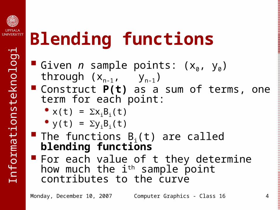
Blending functions Given n sample points: (x0, y0) through (xn-1, yn-

1) Construct P(t) as a sum of terms, one term for

each point: x(t) = xiBi(t) y(t) = yiBi(t)

The functions Bi(t) are called blending functions

For each value of t they determine how much the ith sample point contributes to the curve

Info

rmat

ions

tekn

olog

i


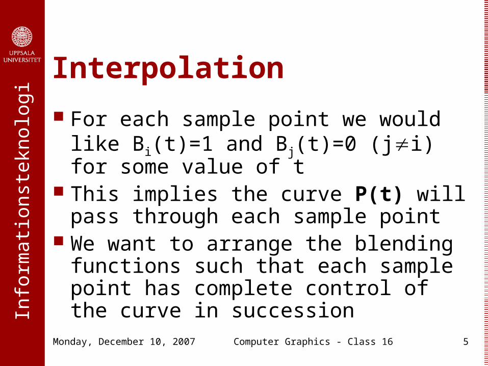
Interpolation

For each sample point we would like Bi(t)=1 and Bj(t)=0 (ji) for some value of t

This implies the curve P(t) will pass through each sample point

We want to arrange the blending functions such that each sample point has complete control of the curve in succession

Info

rmat

ions

tekn

olog

i


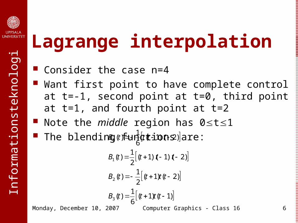
Lagrange interpolation Consider the case n=4 Want first point to have complete control at t=-1, second

point at t=0, third point at t=1, and fourth point at t=2 Note the middle region has 0t1 The blending functions are:

)1()1(6

1)(

)2()1(2

1)(

)2)(1)(1(2

1)(

)2)(1(6

1)(

3

2

1

0

ttttB

ttttB

ttttB

ttttB

Info

rmat

ions

tekn

olog

i


Drawing the curve Vary t in small increments between 0 and 1 This will interpolate the curve between 2nd and 3rd

control points To handle entire curve (more than 4 control points)

draw curve between 2nd and 3rd points as above, then step up one control point and repeat for middle set

For very first set of 4 control points will need to evaluate between t=-1 and t=0

For very last set of 4 control points will need to evaluate between t=1 and t=2

Info

rmat

ions

tekn

olog

i


Program for curve fitting

curves.cpp is available online Program does three curve fitting

techniques Lagrange interpolation Bézier curves Uniform cubic B-spline

Examine general program set-up and interpolation routine now

Info

rmat

ions

tekn

olog

i


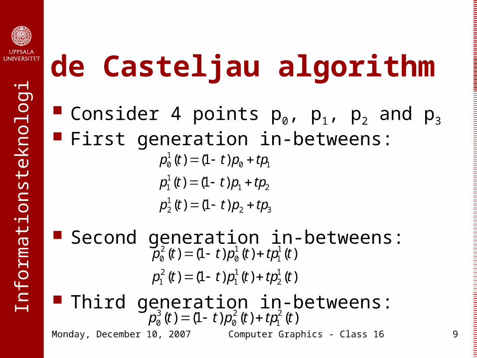
de Casteljau algorithm Consider 4 points p0, p1, p2 and p3

First generation in-betweens:

Second generation in-betweens:

Third generation in-betweens:

3212

2111

1010

)1()(

)1()(

)1()(

tppttp

tppttp

tppttp

)()()1()(

)()()1()(12

11

21

11

10

20

ttptpttp

ttptpttp

)()()1()( 21

20

30 ttptpttp

Info

rmat

ions

tekn

olog

i


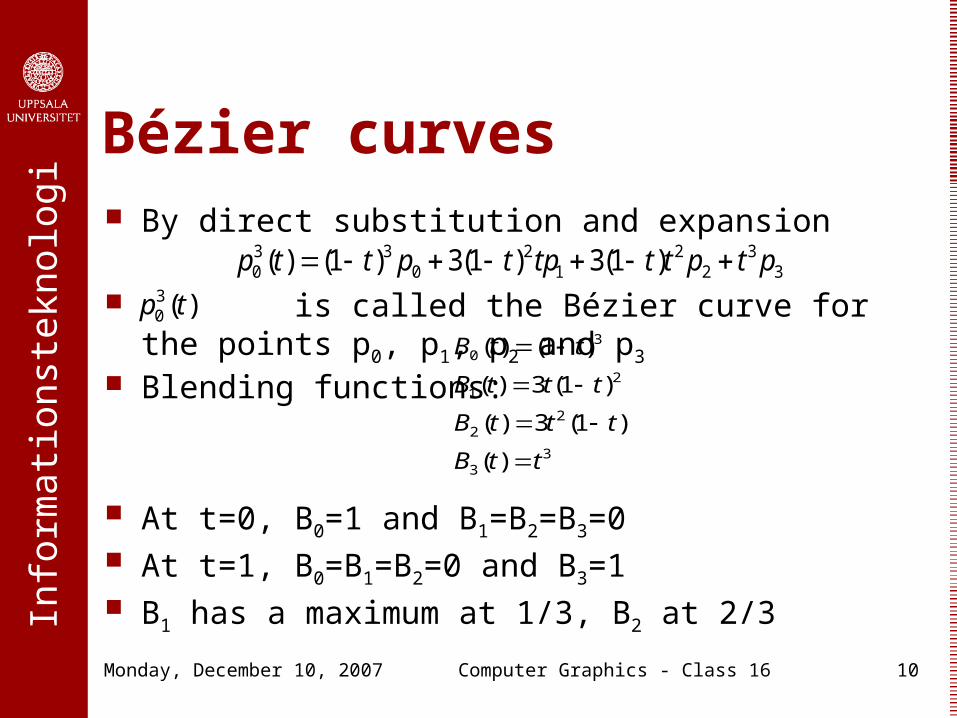
Bézier curves By direct substitution and expansion

is called the Bézier curve for the points p0, p1, p2 and p3

Blending functions:

At t=0, B0=1 and B1=B2=B3=0 At t=1, B0=B1=B2=0 and B3=1 B1 has a maximum at 1/3, B2 at 2/3

33

22

12

033

0 )1(3)1(3)1()( ptptttptpttp )(30 tp

33

22

21

30

)(

)1(3)(

)1(3)(

)1()(

ttB

tttB

tttB

ttB

Info

rmat

ions

tekn

olog

i


Observations on Bézier curves

Pass through p0 and p3 only Can generate closed curves by specifying

first and last control points to be the same A single control point can be specified two

or more times if you want that point to exert more control of the curve in its region

Info

rmat

ions

tekn

olog

i


Complicated Bézier curves More than 4 control points Piece together using smaller order curves with

fewer control points Match endpoints for zero-order continuity At the endpoints, the tangent to the curve is

along the line that connects the endpoint to the adjacent control point; obtain first-order continuity by picking collinear control points (last two of one section with first two of next section - with the endpoints the same)

Info

rmat

ions

tekn

olog

i


Revisit program for curve fitting

Examine Bézier curve fitting routine in curves.cpp

Info

rmat

ions

tekn

olog

i


Splines An mth degree spline function is a piecewise

polynomial of degree m that has continuity of derivatives of order m-1 at each knot

Define the blending functions as shifted versions of the spline function: Bi(t)=B(t-i)

Info

rmat

ions

tekn

olog

i


Cubic splines

Given p0, p1, …, pn, 0t n

Divide into n subintervals [t0, t1], [t1, t2], …, [tn-1, tn]

Approximate points pi by a curve P(t) which consists of a polynomial of degree 3 in each subinterval

Points ti are called knots

Info

rmat

ions

tekn

olog

i


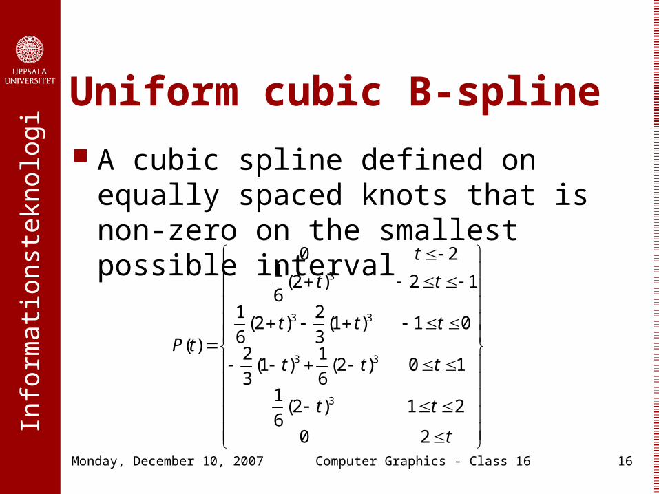
Uniform cubic B-spline

A cubic spline defined on equally spaced knots that is non-zero on the smallest possible interval

t

tt

ttt

ttt

tt

t

tP

20

21)2(6

1

10)2(6

1)1(

3

2

01)1(3

2)2(

6

1

12)2(6

120

)(

3

33

33

3

Info

rmat

ions

tekn

olog

i


Observations on cubic B-splines

At each point at most 4 B-splines are not zero

At a knot only 3 consecutive points affect the curve, with weights 1/6, 2/3, and 1/6 so curve is approximating

If a control point is specified 3 times then curve goes through point as 1/6+2/3+1/6=1

Info

rmat

ions

tekn

olog

i


Revisit program for curve fitting

Examine B-spline fitting routine in curves.cpp

Info

rmat

ions

tekn

olog

i


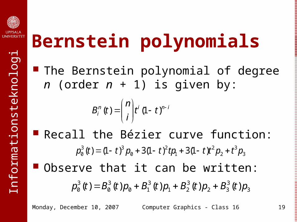
Bernstein polynomials The Bernstein polynomial of degree n (order n +

1) is given by:

Recall the Bézier curve function:

Observe that it can be written:

inini tt

i

ntB

)1()(

33

22

12

033

0 )1(3)1(3)1()( ptptttptpttp

3332

321

310

30

30 )()()()()( ptBptBptBptBtp

Info

rmat

ions

tekn

olog

i


Evaluators An OpenGL mechanism for specifying a curve

or surface using only the control points Use Bernstein polynomials as the blending

functions Can describe any polynomial or rational

polynomial splines or surfaces to any degree, including: B-splines NURBS Bézier curves and surfaces

Info

rmat

ions

tekn

olog

i


Defining an evaluator glMap1d (GL_MAP1_VERTEX_3, 0.0, STEPS, 3, 4, &points[j][0]); one-dimensional evaluator (a curve) specifies x,y,z coordinates (need glEnable(GL_MAP1_VERTEX_3);)

parameter variables goes 0.0 to STEPS 3 indicates number of values to advance in the data

between one control point and the next 4 is the order of the spline (degree + 1) &points[j][0] is a pointer to first control point’s

data

Info

rmat

ions

tekn

olog

i


Evaluating a map

glEvalCoord1d (i); evaluates a map at a given value of the parameter variable

Value of i should be between 0.0 and STEPS

Info

rmat

ions

tekn

olog

i


Example program

evaluator.cpp is an example program using an evaluator

It does a fit of the same data that the curve fitting program did

Info

rmat

ions

tekn

olog

i


Surfaces

The same curve fitting techniques can be extended to surfaces by applying the methods in two dimensions

For example, the Utah teapot is formally defined as a series of 32 bicubic Bézier patches using 306 control points

Info

rmat

ions

tekn

olog

i


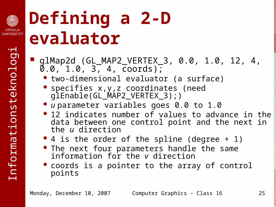
Defining a 2-D evaluator glMap2d (GL_MAP2_VERTEX_3, 0.0, 1.0, 12, 4, 0.0, 1.0, 3, 4, coords); two-dimensional evaluator (a surface) specifies x,y,z coordinates (need glEnable(GL_MAP2_VERTEX_3);)

u parameter variables goes 0.0 to 1.0 12 indicates number of values to advance in the data

between one control point and the next in the u direction 4 is the order of the spline (degree + 1) The next four parameters handle the same information for

the v direction coords is a pointer to the array of control points

Info

rmat

ions

tekn

olog

i


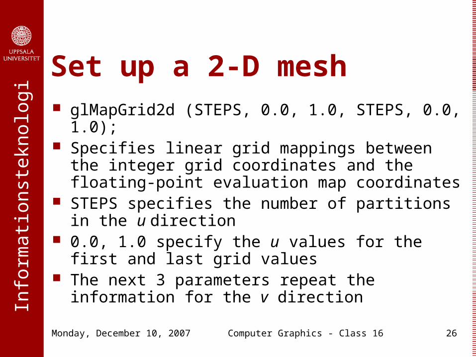
Set up a 2-D mesh glMapGrid2d (STEPS, 0.0, 1.0, STEPS, 0.0, 1.0);

Specifies linear grid mappings between the integer grid coordinates and the floating-point evaluation map coordinates

STEPS specifies the number of partitions in the u direction

0.0, 1.0 specify the u values for the first and last grid values

The next 3 parameters repeat the information for the v direction

Info

rmat

ions

tekn

olog

i


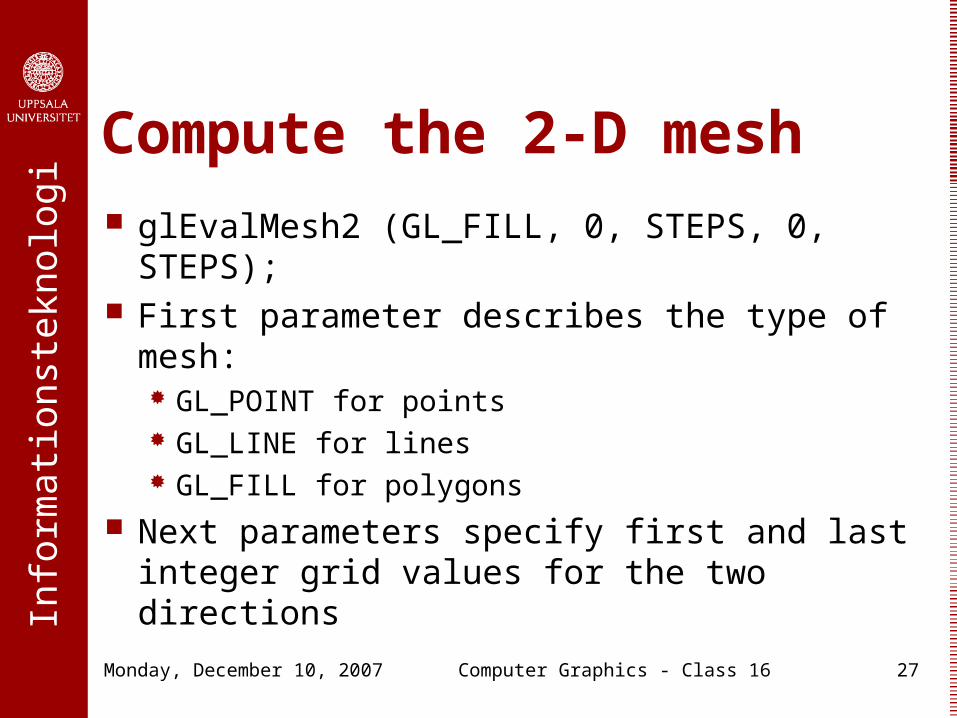
Compute the 2-D mesh glEvalMesh2 (GL_FILL, 0, STEPS, 0, STEPS);

First parameter describes the type of mesh: GL_POINT for points GL_LINE for lines GL_FILL for polygons

Next parameters specify first and last integer grid values for the two directions

Info

rmat

ions

tekn

olog

i


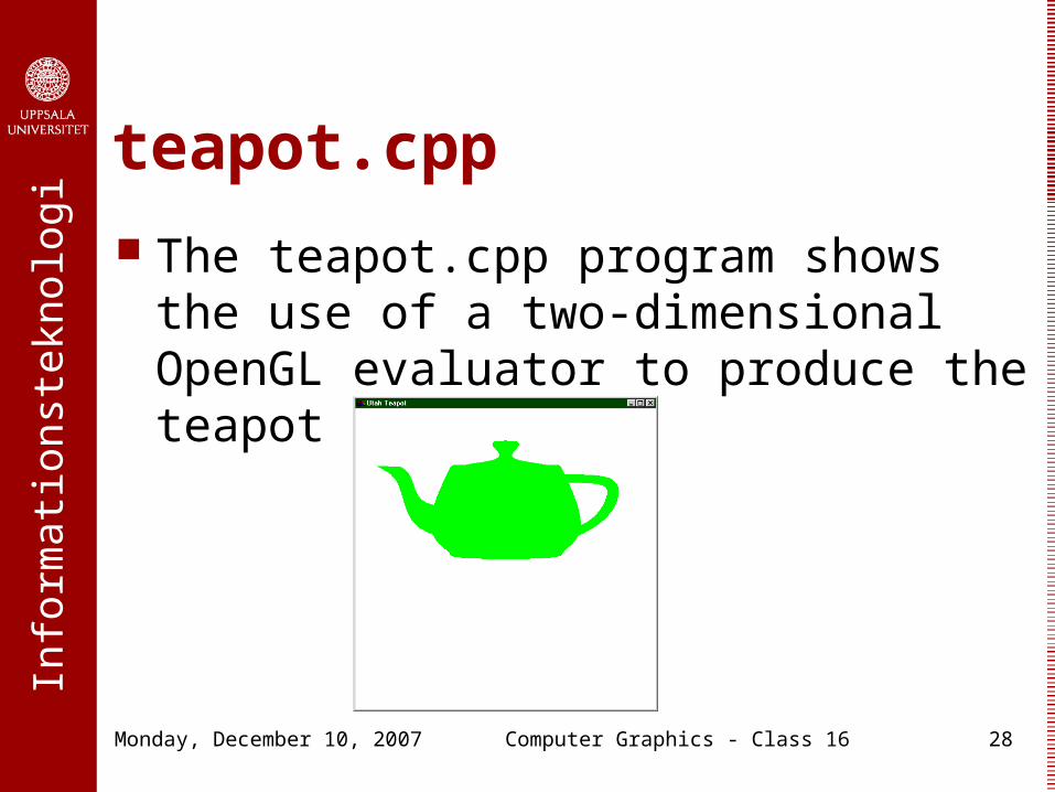
teapot.cpp

The teapot.cpp program shows the use of a two-dimensional OpenGL evaluator to produce the teapot

Documents

Informationsteknologi Monday, December 10, 2007Computer Graphics - Class 161 Today’s class Curve fitting Evaluators Surfaces