Embed Size (px)
Citation preview

JRC TECHNICAL REPORTS
A Distributed Approach to solvePower Flow problems in newemerging scenarios
Methodological aspects,implementation issuesand applications
Rinaldo, S. G., Ceresoli, A., Prettico, G.
2019
EUR 29998 EN
Report EUR xxxxx EN
20xx
Forename(s) Surname(s)
First subtitle line first line
Second subtitle line second
Third subtitle line third line
First Main Title Line First Line
Second Main Title Line Second Line
Third Main Title Line Third Line

This publication is a Technical report by the Joint Research Centre (JRC), the European Commission’s scienceand knowledge service. It aims to provide evidence-based scientific support to the European policymakingprocess. The scientific output expressed does not imply a policy position of the European Commission. Neitherthe European Commission nor any person acting on behalf of the Commission is responsible for the use thatmight be made of this publication.
Contact InformationName: S. G. Rinaldo, A. Ceresoli, G. PretticoAddress: Joint Research Centre, Via Enrico Fermi 2749, TP 044, 21027 Ispra (VA), ItalyE-mail: [email protected]
EU Science Hubhttps://ec.europa.eu/jrc
JRC116302
EUR 29998 EN
PDF ISBN 978-92-76-11252-5 ISSN 1831-9424 doi:10.2760/869640
Luxembourg: Publications Office of the European Union, 2019
© European Union, 2019
The reuse policy of the European Commission is implemented by Commission Decision 2011/833/EU of 12December 2011 on the reuse of Commission documents (OJ L 330, 14.12.2011, p. 39). Reuse is authorised,provided the source of the document is acknowledged and its original meaning or message is not distorted. TheEuropean Commission shall not be liable for any consequence stemming from the reuse. For any use orreproduction of photos or other material that is not owned by the EU, permission must be sought directly fromthe copyright holders.
All content © European Union, 2019, except: Front page image. 2019. Source: [Fotolia.com]
How to cite this report: Rinaldo, S., Ceresoli, A. and Prettico, G., A Distributed Approach to solve Power Flowproblems in new emerging scenarios, EUR 29998 EN, Publications Office of the European Union, Luxembourg,2019, ISBN 978-92-76-11252-5 (online), doi:10.2760/869640 (online), JRC116302.


A Distributed Approach to solve Power Flow problems
in new emerging scenarios

Contents
Acknowledgements............................................................................................................. 1
1 Introduction .................................................................................................................... 4
1.1 Broad Context .......................................................................................................... 4
1.2 Project Context ........................................................................................................ 5
1.3 Project Scope ........................................................................................................... 6
1.4 Organisation ............................................................................................................. 7
2 Power Flow, Numerical Methods & Distributed Power Flow Methodology .......... 8
2.1 Electrical Variables, Grid Components, Bus Types ........................................... 8
2.2 The Power Flow Problem........................................................................................ 9
2.3 Non-Linear Solvers for Power Flow Equations................................................... 11
2.3.1 Newton-Raphson .............................................................................................. 12
2.3.2 Newton-Raphson with Line Search ............................................................... 18
2.4 Introduction to Linear Solvers .............................................................................. 19
2.4.1 Direct Methods .................................................................................................. 19
2.4.2 Iterative Methods & Preconditioning ............................................................ 20
2.4.3 Practical Updating Schemes & Basic Implementation Algorithms .......... 24
2.4.4 Computational Complexity of Direct and Iterative Methods.................... 28
2.5 Iterative Methods, Distributed Power Flow & Current Practices .................... 32
2.5.1 Current Practices and Iterative Methods in Power Flow ........................... 32
2.5.2 Distributed Approaches ................................................................................... 33
2.5.3 Krylov-Schwarz Methods & Distributed Computation of Power Flow ..... 34
2.5.4 Distributed Power Flow.................................................................................... 43
3 PETSc ............................................................................................................................... 46
3.1 PETSc Structure....................................................................................................... 46
3.2 PETSc representation of networks: DMNetwork and DMPlex ........................ 47
3.3 Solving Power Flow Equations using PETSc ....................................................... 49
4 Distributed Power Flow in PETSc ................................................................................ 54
4.1 Introduction.............................................................................................................. 54
4.2 Parallel communication analysis of set up phase in PETSc ............................ 54
4.3 Parallel Assembling procedure.............................................................................. 56
4.4 Solving Phase........................................................................................................... 57
i

5 Applications .................................................................................................................... 62
5.1 Congestion Management at European Level ..................................................... 62
5.1.1 CA and CC: History and Implementations .................................................. 63
5.1.2 Relevant CACM articles.................................................................................... 64
5.1.3 Capacity Calculation Mechanisms: ATC ....................................................... 66
5.1.4 Capacity Calculation Mechanisms: Flow Based.......................................... 68
5.1.5 Limitation of Current Practices ...................................................................... 71
5.1.6 Advantages of Distributed Capacity Calculation ........................................ 74
5.2 TSO-DSO Coordination .......................................................................................... 75
5.2.1 Operational & Policy Context in Distribution Grid Management ............. 75
5.2.2 TSO-DSO Current Cooperation ...................................................................... 76
5.2.3 TSO-DSO interface with distributed approach ........................................... 77
6 Conclusions & Future Works........................................................................................ 78
References............................................................................................................................ 80
List of abbreviations and definitions ............................................................................... 84
List of figures ....................................................................................................................... 86
List of tables ........................................................................................................................ 87
Annexes ................................................................................................................................ 88
Annex 1. Ybus ................................................................................................................. 88
Annex 2. GMREs.............................................................................................................. 88
Annex 3. Installing the Software ................................................................................. 88
Annex 4. Setting up a small cluster computing environment ............................... 89
Annex 5. Running the Distributed Power Flow Simulations ................................... 91
ii

Acknowledgements
We would like to thank all the colleagues of the C.3. unit - Energy Security, Distribution andMarkets - for the support and sharing of precious scientific insights. We also thank Professor D.J.P.Lahaye of TU Delft and Professor M. Merlo of Politecnico of Milano for the trustworthy feedbackand valuable advice in conducting this research work.
AuthorsStefano Guido Rinaldo, Andrea Ceresoli, Giuseppe Prettico
1

Abstract
Distributed Computing is growing up in interest in many applied fields of scientific research. Atthe same time power system operation is becoming increasingly complex due to the need to integratea relevant amount of energy production coming from Distributed Energy Resources (DERs) connectedat various voltage levels. In this context, the need to automate grid operations is in fact fundamentalto ensure adequate levels of reliability, flexibility and cost effectiveness of power systems. This reportprovides methodological aspects and principles for the solution of the power flow problem througha distributed approach. The focus is on the case in which multiple interacting entities (utilities) bysharing a small portion of their grids data with the other parties can improve the solution of theglobal grid (composed by all the grids involved). The advantage is that the computation is donelocally and in parallel with the others without the need to exchange further data. The aim of thisreport is both to give the reader a comprehensive overview of the software used for the implementa-tion, the Portable Scientific Extensible Toolkit for Scientific Computation (PETSc), and to highlightthe principles followed to build the Distributed Power Flow Solver as well as the specific featuresthat diversify our approach from others. Finally, two case studies are presented as potential appli-cations of our model: the capacity calculation between transmission system operators (TSOs), andthe transmission-distribution networks coupling between TSOs and Distribution System Operators(DSOs). Open issues and future research studies are discussed in the final part of the present report.
2

3

1 Introduction
1.1 Broad Context
Power systems are one of the most complex engineering human-made works. Operating sucha sophisticated system requires constant monitoring, high-automation level, continuous correctiveactions and planning as close as possible to real-time. In recent years power systems have been facingan arising number of challenges set by the on-going energy transition. In Europe, this has been mainlydriven by European Commission (EC) energy policies (Third Energy Package - TEP, 2009 and CleanEnergy Package - CEP, 2018) that have set important goals for carbon emission reduction and marketharmonisation1 for the member states (MS).
In the past national grids were designed to serve the same scope: that of transmitting electricityproduced in big centralised power plants to final consumers at different voltage levels. The power wasused to flow solely from generating plants to final consumers passing through meshed transmissionnetworks and radial distribution networks. All grid-related activities were fully under the responsibilityof national Transmission System Operators (TSOs), while the distribution grid was built according toa fit-and-forget approach, over-staffed and with passive role. At market level, no competitive auctionswere in place (e.g. through a power exchange pool) and all the stages of the electricity supply chainwere managed by a single vertical integrated company. This plain and simple organisation of theelectricity supply chain ensured an easy and reliable operation of the grid in the past, even thoughsupposedly not in the most economically efficient manner. Moreover this approach proved not suitableto match the novel ways of consuming and producing electricity.
These reasons have led to a radical re-engineering of the power sector in the last couple of decades.The complete unbundling of generation electricity companies from transmission sector realised by theTEP resulted in the introduction of competitive market designs (the Power eXchanges - PXs) atwholesale level. In practical terms, this allows to auction the use of the grid together with theenergy trade and reward the less costly generators with network access. This new paradigm forelectricity markets from one hand increases market liquidity, lowers prices and provides a frameworkfor more transparent trades. On the other hand, unbundling makes the operation of power systemsmore complex. Generating companies, system operators, market operators and suppliers must allcoordinate with each other and continuously exchange information in order to ensure the security ofsupply and the efficient management of the power system as a whole.
At the same time in order to cope with a drastic reduction of the carbon emissions, powergeneration must shift from conventional fossil-based technologies to Renewable Energy Sources (RES).The power production from RES is typically dislocated over the grid and connected at different voltagelevels, often at medium and low voltage levels (MV-LV). Furthermore, new actors are entering thecompetitive markets (e.g. prosumers) and new type of loads are challenging the stability of thesystem (e.g electric vehicles (EVs)). The intermittent and stochastic nature of such DistributedEnergy Resources (DERs) is strongly influencing the grid operation, as the increasing uncertainty onflows prediction and real-time grid state, especially at distribution level, makes it difficult to ensuresecurity of supply and efficient optimisation of resources. In other words, TSOs see volatile flowsappearing on their system as a result of the real-time uncertain behaviour of DERs at distributionlevel and hence are moved to procure more often system services (e.g. balancing, voltage support)and called for corrective actions. At distribution level, investments in proper control systems andmonitoring infrastructure will become necessary.
To summarise, future power systems have to withstand both the uncertainties and complexitiesintroduced by DERs at operation level, providing a reliable and cost efficient service, while ensuring
1From this point of view, the final goal is to create a fully harmonised Internal Energy Market (IEM) in Europe,offering one single wholesale price for all member states.
4

the unbundling at different stages of electricity supply chain. In this context, where economic andoperational challenges might look in anti-thesis, the integration of smart and intelligent devices aswell as of innovative methodologies for power system analyses play a pivotal role.
1.2 Project Context
Distributed computing is applied in a great number of different research and industry contexts.The growing importance of distributed computing is mainly related to the advantages of de-centralisedapproaches, typically allowing to better exploit computational resources otherwise not used, to re-duce investments, to keep data-locality and to be fault-tolerant. Among the aforementioned appealingfeatures of distributed applications, the application presented in the following focuses on input data-locality. This report discusses the methodology to carry out a distributed solution of power flowequations and gives guidance on the chosen implementation based on the parallel computing soft-ware (PETSc). The framework under study is that of cross-border flow exchanges. In this context,distributed approaches might find application every time that coordination is needed among systemoperators managing different parts of a global inter-connected grid. The application aims at automat-ing such a coordination, by only providing local data as input to the power flow simulation. On thispurpose, we focus here on two situations: at member states level (thus among neighbouring Euro-pean countries i.e. at the transmission level) and at national level (at the transmission-distributioninterface). A brief description of the current state of the art for both levels is depicted in the following.
At the transmission level, investments in expanding cross-border capacities are one of the maintopic of the recently published CEP2. This will enable more frequent exchanges of electricity anda more flexible operation between member states. For instance, in cases of unexpected surplus ofelectricity or in order to be able to cover shortfalls as a result of the unpredictability of RES (windand solar) national TSOs might rely on neighbouring countries at need. The creation of a propermarket design at European level that reflects such exchanges and allocate efficiently cross-borderrights is thus needed. At national level cross-border exchanges at day-ahead (DAM) and intra-day (IDM) markets3 were firstly organised so that capacity and energy were bid explicitly (i.e. indifferent markets) over different time-frames. However this is not economically efficient, since thoseagents that procure cross-border capacity ex-ante can exert market power on the spot markets, oftencausing the prices to increase. Moved by this reason, three European PXs (OMEL, NORDPOOLand EPEX Spot) launched in 2009 the Price Coupling of Regions (PCRs) project, an initiative topromote coordinated (implicit) price formation on their respective spot markets. In other words,grid constraints are modelled into the price formation algorithm and, as the market clears, quantityand prices formed are those that maximise welfare subject to grid constraints. Nowadays, the PCRproject involves eight PXs. The market is cleared by solving the market problem centrally, through theEUPHEMIA algorithm.4 To clear the DA problem, EUPHEMIA needs a set of pre-calculated inputs.TSOs closely coordinate with each other and with Nominated Electricity Market Operators (NEMOs)in order to model the grid constraints and find compatible market equilibrium. The procedure tomodel cross-border interconnections takes place through a complex and long procedure made up ofseveral steps that conceptually could be simplified into two main ones: 1) a Capacity Calculation (CC)
2When we refer to the CEP we refer mainly to the Electricity Regulation (Ele, 2019b) and to the Electricity Directive(Ele, 2019a)
3From now on we refer to DAM and IDM as spot markets. According to finance terminology, spot markets arethose markets that involve the trading of financial instruments for immediate delivery, in contrast with forward markets,where trade refers to future delivery. Although DAM and IDM are not strictly spot markets, in the electricity sectorthey are commonly referred to as such.
4EUPHEMIA stands for Pan-European Hybrid Electricity Market Integration Algorithm. EUPHEMIA clears theday-ahead market over Europe for more than 50 bidding zones, allocating cross-border transmission capacity for morethan 60 inter-connectors in less than 10 minutes.
5

procedure requiring TSOs coordination; and 2) a Capacity Allocation (CA) mechanism requiring acommon market clearing algorithm. During these steps system operators run several times power flowcomputations, in order to calculate parameters, to define physical limits for electrical components,toforesee contingencies, etc. In this work we focus on step 1, even though distributed approaches canin principle be thought also for step 2.
At national level the framework is considerable different. Even though long-run investments areincreasingly being planned, distribution grids’ observability and controllability are still very limited(Prettico et al., 2019). The uncertainty of RES production connected at MV-LV levels thus translateinto volatile flows at transmission level. Nowadays, TSO and DSOs exchange information about thestate of their grids periodically (even though this periodicity differs considerably among MS), thoughnot carrying out coordinated calculations. As a result, TSOs need to estimate the uncertainty ongeneration and demand pattern down to lower voltage levels and procure balancing reserves ex-anteto account for worst-case scenarios. From the DSOs side, even though the grid is over-staffed,congestions may occur caused by the increasing penetration of RES. In this context we foresee thatsoon DSOs will collect more detailed and fine grained information and will run power flow equationsto improve their knowledge of the actual state of their grids. The inherent uncertainty from DSO toTSO might be mitigated by allowing a coordinated calculation framework for TSO and DSOs thatprovide data-locality and hence do not prejudice competition.
1.3 Project Scope
This report discusses methodologies, issues and applications of an experimental distributed powerflow solver. The aim is to carry out a distributed computation of the load flow problem between twoseparated parties (bipartite case) sharing a grid boundary. In other words, the goal is to provide twogrid operators (TSO-DSO or TSO-TSO) with an application capable of performing exact load flowcomputations on a joint network by exchanging only a limited piece of information (for instance thatat the interfacing nodes between the two networks). This is in line with unbundling policy indicationsand operational issues briefly presented in 1.1 and 1.2. The application framework investigated is thusthat one of cross-border exchanges, among national EU countries, through transmission-distributioninterface, or in general among adjoining grid operators. The implementation takes advantage of thePortable Extensible Toolkit for Scientific Computation (PETSc), an API (Application ProgrammingInterface) for writing parallel scientific applications based on the C programming language. Forthe sake of completeness, we chose to dedicate a whole chapter to the understanding of PETScfunctionalities (Section 3), in order to provide the reader with an overview of the software and tobuild up increasing layers of complexities step-by-step.
6

1.4 Organisation
This report may be conceptually broken down into four parts. The first part reviews the powerflow problem and solvers. Then, the mathematical methodology to compute the power flow equationsremotely is introduced. The second part introduces the reader to the PETSc API, providing itsgeneral functioning. In the third part, based on the concepts introduced in Section 2 and Section3, we explain the Distributed Power Flow. Finally, the last part shows two proposed applicationsframeworks (transmission-transmission interface, transmission-distribution interface).
A more detailed overview of the report organisation is provided in the following.
Section 2 starts from recalling power system basics and the power flow problem. Later, we graduallyintroduce more complex solvers for the PF equations, reviewing pros and drawbacks. Linearsolvers and parallel implementation become the central topic of discussion during the secondpart of this section. A short section is dedicated to parallel communication analysis of station-ary block preconditioned solvers. In the final part, we provide an example of the distributedmethodology on case13.m by using the Newton-Krylov-Schwarz (NKS) approach.
Section 3 introduces to the use of the Portable Extensible Toolkit for Scientific Computation (PETSc).This chapter provides a quick hand-guide to the PETSc API and discuss its relevance in thiswork.
Section 4 discusses the implementation of the Distributed Power Flow in PETSc.
Section 5 provides an in-depth review of two possible fields of application for the distributed method-ology: 1) In the context of congestion management at European level, and specifically on thecapacity calculation process for transmission-transmission flow control; 2) In the context oftransmission-distribution network coupling, touching upon the TSO-DSO interaction.
Section 6 draws conclusions and possible future works on power flow distributed solvers.
7

2 Power Flow, Numerical Methods & Distributed PowerFlow Methodology
In this chapter the relevant electrical variables, the formulation of the power problem (or loadflow) and the main numerical methods that are used in the current transmission system operatorpractice are presented. This background information will turn out useful in the next chapters whenthe distributed power flow methodology is presented. It is worth mentioning that the aim of thissection is not to carry out an extensive review of the mathematical methods used to solve powerflow equations, but rather to provide a concise background to the reader willing to grasp the morecomplex features of the distributed methodology.
2.1 Electrical Variables, Grid Components, Bus Types
In this section we introduce the relevant electrical variables for the formulation of the powerflow problem and the classification of buses, in line with regular TSOs practices. In AC operation,electricity is an oscillating flow of electrons at a certain constant frequency5. As a result, current,voltage and complex power are time-variant quantities that might be difficult to deal with whenwriting down equations for grid modelling. Furthermore, in steady-state analysis there is no interestin knowing the instant values of those variables, but rather to assess some difference among them(e.g. nodal voltage difference, current-voltage difference, etc.). For these reasons, for steady-stategrid analysis, electrical variables are defined through phasors. Phasors are rotating vectors in thecomplex plane that are used to represent time variant oscillating electrical quantities. Phasors allowto split the information needed to assess an electrical variable into just two components, the phaseand the module. Thus, let us define the following parameters:
The current phasor: I = IejδI = I(cosδI + jsinδI)
The voltage phasor: V = V ejδV = V (cosδV + jsinδV )
The complex power phasor: S = Sejϑ = S(cosθ + jsinθ)
From now on we refer to V as the voltage magnitude and to δV as the voltage angle. Notethat the complex power S is related to the active power P and reactive power Q by the followingexpression:
S = P + jQ (1)
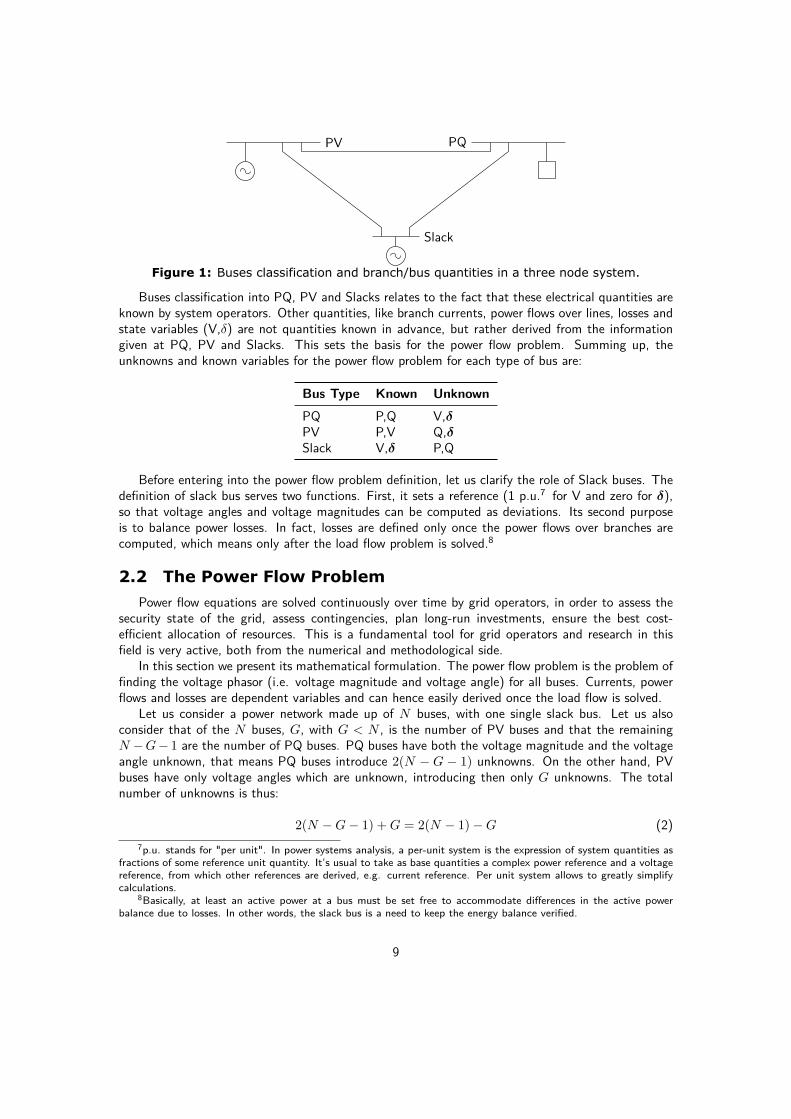
Electrical grids may be modeled in many ways. From the mathematical point of view an electricgrid can be interpreted as a graph G(B, E), where B and E denote the set of buses and edgesrespectively and G is a mapping between B and E providing the connectivity bus-edges6. From anengineering and operating side, a power grid is an interconnected network of components that aim atmoving electricity from generators to final consumers. Buses act as sinks, injecting or withdrawingpower to/from the grid, while edges (i.e. transmission/distribution lines) allow for transportation. Assuch, electric variables may be branch related or bus related. In this work, we refer to bus variableswith capital letters and to branch variables with lowercase letters. Buses can be categorised into threetypes: those that provide net injections to the grid (PV buses); those that make net withdrawals fromthe grid (PQ buses); those that have flexible operation and thus compensate for losses (called Slackbuses) (see Fig. 1).
5In Europe the oscillating frequency is 50Hz.6PETSc extensively makes use of graph theory to store and manage networks. This is shortly deepened in Section
4 and contextualized in power flow.
8
PV PQ
Slack
Figure 1: Buses classification and branch/bus quantities in a three node system.
Buses classification into PQ, PV and Slacks relates to the fact that these electrical quantities areknown by system operators. Other quantities, like branch currents, power flows over lines, losses andstate variables (V,δ) are not quantities known in advance, but rather derived from the informationgiven at PQ, PV and Slacks. This sets the basis for the power flow problem. Summing up, theunknowns and known variables for the power flow problem for each type of bus are:
Bus Type Known UnknownPQ P,Q V,δPV P,V Q,δSlack V,δ P,Q
Before entering into the power flow problem definition, let us clarify the role of Slack buses. Thedefinition of slack bus serves two functions. First, it sets a reference (1 p.u.7 for V and zero for δ),so that voltage angles and voltage magnitudes can be computed as deviations. Its second purposeis to balance power losses. In fact, losses are defined only once the power flows over branches arecomputed, which means only after the load flow problem is solved.8
2.2 The Power Flow Problem
Power flow equations are solved continuously over time by grid operators, in order to assess thesecurity state of the grid, assess contingencies, plan long-run investments, ensure the best cost-efficient allocation of resources. This is a fundamental tool for grid operators and research in thisfield is very active, both from the numerical and methodological side.
In this section we present its mathematical formulation. The power flow problem is the problem offinding the voltage phasor (i.e. voltage magnitude and voltage angle) for all buses. Currents, powerflows and losses are dependent variables and can hence easily derived once the load flow is solved.
Let us consider a power network made up of N buses, with one single slack bus. Let us alsoconsider that of the N buses, G, with G < N , is the number of PV buses and that the remainingN −G− 1 are the number of PQ buses. PQ buses have both the voltage magnitude and the voltageangle unknown, that means PQ buses introduce 2(N − G − 1) unknowns. On the other hand, PVbuses have only voltage angles which are unknown, introducing then only G unknowns. The totalnumber of unknowns is thus:
2(N −G− 1) +G = 2(N − 1)−G (2)7p.u. stands for "per unit". In power systems analysis, a per-unit system is the expression of system quantities as
fractions of some reference unit quantity. It’s usual to take as base quantities a complex power reference and a voltagereference, from which other references are derived, e.g. current reference. Per unit system allows to greatly simplifycalculations.
8Basically, at least an active power at a bus must be set free to accommodate differences in the active powerbalance due to losses. In other words, the slack bus is a need to keep the energy balance verified.
9

The same number of equations (not introducing other unknowns) is needed in order to obtain aunique solution for the mentioned problem. In principle, there’s no constraining rule upon the choiceof these equations. The most common choice is to write nodal power mismatch equations: we canwrite the active power balance equation for each PQ and PV buses, for a total of N − 1 equations.Then we can write a reactive power balance equation for each PQ bus (i.e. N − G − 1), getting atotal number of equations of:
N −G− 1 +N − 1 = 2(N − 1)−G (3)Which is equal to the number of unknowns. Let us write them down explicitly for the generic bus
i. This is done starting from the net complex power expression injected or withdrawn from bus i:
Si = ViIi (4)Where Vi, Ii are the bus voltage and bus current related to the bus i. Notice that the underline
of I stands for the complex conjugate operator. The nodal current I may be expressed in terms ofincident branch currents by introducing the Kirchhoff’s Current Law (KCL). The KCL states that thecharge flow cannot be generated, consumed or collected in a bus, so that the current summation ata node must be zero. In other terms, we can express I as:
I =m∑j=1
i (5)
Where m is the number of incident buses at bus i. By introducing Eq.(5) into Eq.(4) we obtain:
Si = Vi
m∑j=1
ij (6)
The currents ij are unknowns. Introducing the Ohm’s Law we can express them in terms ofcomplex voltages obtaining:
Si = Vi
N∑j=1
YijVj (7)
Where Yij is the ij element of the nodal admittance matrix (see Annex 1). According to thecomplex expressions introduced in 2.1, the phasors can be expanded as followss:
Si =N∑j=1
ViVjYijej(δi−δj−θij) (8)
Being Eq.(8) a complex equation, it can be separated into its scalar components:
Pi =N∑j=1
ViVjYij cos (δi − δj − θij) (9)
Qi =N∑j=1
ViVjYij sin (δi − δj − θij) (10)
These are the so-called power flow equations. Note that we are dealing with nodal quantities,that means, that the δi, δj are voltage angles related to bus i and j. Whilst θij refers to the phaseshift given by line parameters connecting bus i with bus j.
10

The power flow equations relate grid state variables with net injection/withdrawals Pi, Qi. Sincein reality, grid operators know the scheduled generation profiles and the demand forecasts, it can besaid that Pi, Qi are known inputs for their power flow computations. Additionally, the grid operatorsown all the data about components connected to the grid, e.g. switches state, lines parameters,bus-edges connectivity (i.e. topology). In other words, the only unknowns are the state variablesV, δ.
Before introducing the solution methods, let us derive an alternative but equivalent formulationof the power flow equations. Let us consider Eq.(7) and separate the admittance matrix Yij in itsreal and imaginary components Gij , Bij . This translates into:
Si = ViIi = Vi
N∑j=1
YijVj =N∑j=1
ViVj(Gij − jBij)(cos δij + j sin δij) (11)
And by separating active and reactive power components:
−Pi +N∑j=1
ViVj(Gij cos δij +Bij sin δij) = 0
−Qi +N∑j=1
ViVj(Gij sin δij −Bij cos δij) = 0
(12)
This alternative formulation is the one used in the distributed solver discussed in this work. Thepower flow problem is thus a system of non-linear algebraic equations. In other words, Eq.(12) belongsto the general class of problems:
F(x) = 0 with x =[Vδ
]=
V1...
VPQδ1...
δP Q+P V
(13)
Practically speaking this means to look for the roots vector x of the non-linear vector-valuedfunction F. Note that all bold quantities refer to vectors. Finding the roots of an algebraic nonlinearsystem of equations is not an easy task. Exact (i.e. analytical) solutions exist only for special cases.For all the other cases since this is not possible the solution is investigated through numerical methods.The next sections introduce the numerical approaches used to solve the power flow problem. Thishas a double aim. From one side, to review the reference methods in the industry practice, fromthe other side, to establish a basis for the mathematical approach here proposed to carry out thedistributed power flow computation.
2.3 Non-Linear Solvers for Power Flow Equations
All over the world industry practice, power flow equations are solved by means of a quite standardapproach. An iteration procedure is started to approximate the non-linear problem to a linear one.Then, the arising linear system is further simplified through a factorisation technique and solved inone single step. The procedure restarts as a stopping criteria is fulfilled. This approach combines a
11
non-linear Newton step with a direct single-step method, giving a good balance between robustnessand computational time, which motivates the long-time reference of the industry practice9.
Research in numerical solution of power flow equations has in recent years explored outer-inneriterative methods as well. This approach combines a Newton iteration and an iterative linear proce-dure. These methods very often offer good parallel features, better scalability and possibility to berun on distributed platforms.
In the following sections we start by reviewing the Newton’s method, moving then to linearsolvers, and later to the introduction of a particular numerical approach - the Newton-Krylov-Schwarzalgorithm - available in the PETSc libraries and used for a distributed computation of power flowequations.
2.3.1 Newton-Raphson
The Newton-Raphson (NR) method is a standard approach for many classes of non-linear prob-lems. The NR iterative procedure is quite straightforward: given a starting point for the iteration,the problem is approximated locally to a linear problem, solved, and iterated back. The NR iterationscheme can be expressed in general as:
x(k+1) = x(k) + ∆x(k) (14)
Where the term ∆x(k) works as a "corrective" term at each step k. Hence, the convergence willdepend from ∆x(k).
Solving Monodimensional Case
For sake of clarity, let us first derive the NR method for a single algebraic non-linear equation.We want to find the zero of a function f(x) : R → R in the single variable x, that means to find xsuch that:
f(x) = 0 (15)
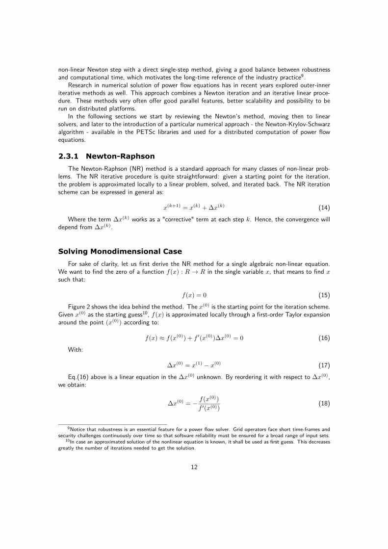
Figure 2 shows the idea behind the method. The x(0) is the starting point for the iteration scheme.Given x(0) as the starting guess10, f(x) is approximated locally through a first-order Taylor expansionaround the point (x(0)) according to:
f(x) ≈ f(x(0)) + f ′(x(0))∆x(0) = 0 (16)
With:
∆x(0) = x(1) − x(0) (17)
Eq.(16) above is a linear equation in the ∆x(0) unknown. By reordering it with respect to ∆x(0),we obtain:
∆x(0) = − f(x(0))f ′(x(0))
(18)
9Notice that robustness is an essential feature for a power flow solver. Grid operators face short time-frames andsecurity challenges continuously over time so that software reliability must be ensured for a broad range of input sets.
10In case an approximated solution of the nonlinear equation is known, it shall be used as first guess. This decreasesgreatly the number of iterations needed to get the solution.
12

Figure 2: Newton-Raphson method for one-dimensional case
So that the next root x(1) is found as:
x(1) = x(0) − f(x(0))f ′(x(0))
(19)
Generalising at iteration k, Eq.(19) becomes:
x(k+1) = x(k) − f(x(k))f ′(x(k))
(20)
Note that, each f ′(x(k)) must never be equal to zero (i.e. no stationary points have to beencountered) in order to get to convergence.
Solving Multidimensional Cases
In the following , we extend the concept to a system of equations. A system of non-linear equationsis defined as a system of generic equations n inm unknowns, where at least one equation is non-linear.In this work, we consider only well-posed problems where the number of equations equal the numberof unknowns (i.e. n = m) and all equations are non-linear. Furthermore, we consider the dense case,where each equation shows dependence on any unknown xi. We will introduce the sparsity later on,where the Newton methodology will be applied to the power flow problem.
A system of non-linear equations is defined as:f1(x1, . . . , xn) = 0f2(x1, . . . , xn) = 0. . . . . . . . . . . .fn(x1, . . . , xn) = 0
More concisely:
13

f(x) =
f1(x)f2(x)...
fn(x)
with x = (x1, . . . , xn)
As the vector-valued function. The solution of a system of non-linear equations can be thusinterpreted as:
f(x) = 0
Which means once again to find the zero vector of the non-linear vectorial function f. This is thesame form obtained in the mono-dimensional case, hence, the same procedure seen in the previousparagraph can be applied, taking into account that in this case scalar variables are substituted byvectors 11. Using the same approach of the mono-dimensional case, we get:
f(x) =
f1(x(k+1))f2(x(k+1))
...fn(x(k+1))
≈f1(x(k)) + ∇f1(x(k)) ·∆x(k) = 0f2(x(k)) + ∇f2(x(k)) ·∆x(k) = 0
......
...fn(x(k)) + ∇fn(x(k)) ·∆x(k) = 0
(21)
And each equation is solved with respect to ∆x(k), whereas fi(x(k)) and ∇fi(x(k)) (with i =1, . . . , n) are evaluated by means of the solution of the previous iteration.
x(k+1) = x(k) − f(x(k))∇f(x(k))
(22)
Exactly as for the mono-dimensional case. Note that the operator ∇ is the gradient operator.This means that the term ∇f(x(k)) is actually a matrix defined as:
J =
∇f1(x)∇f2(x)
...∇fn(x)
=
∂f1∂x1
∂f1∂x2
. . . ∂f1∂xn
∂f2∂x1
∂f2∂x2
∂f2∂xn...
. . ....
∂fn
∂x1
∂fn
∂x2
∂fn
∂xn
(23)
The coefficient matrix J is called Jacobian matrix and it is the matrix of all first order partialderivatives. Therefore, the solution of equations contained in Eq.(21) with respect to ∆x(k) impliesto solve the linear system:
−J(x(k))∆x(k) = f(x(k)) (24)
Note the important result obtained: the non linear problem has been turned into a succession ofk linear systems.
In principle, the solution of Eq.(24) can be approached analytically (if the Jacobian matrix isinvertible, i.e. det(J) 6= 0). By inverting J the exact solution x is found. In practice, this becomessoon unfeasible even for relatively small linear systems (i.e. > 101 unknowns). Let n be the orderof J , calculating its inverse requires O(n!) FLOPS (Floating Point Operation Per Second). Table 1shows how the computational complexity of the problem scales up quickly by solving linear systemsof increasing size, and its relation with computational time.
11Notice that the operator < · > is the dot-product.
14
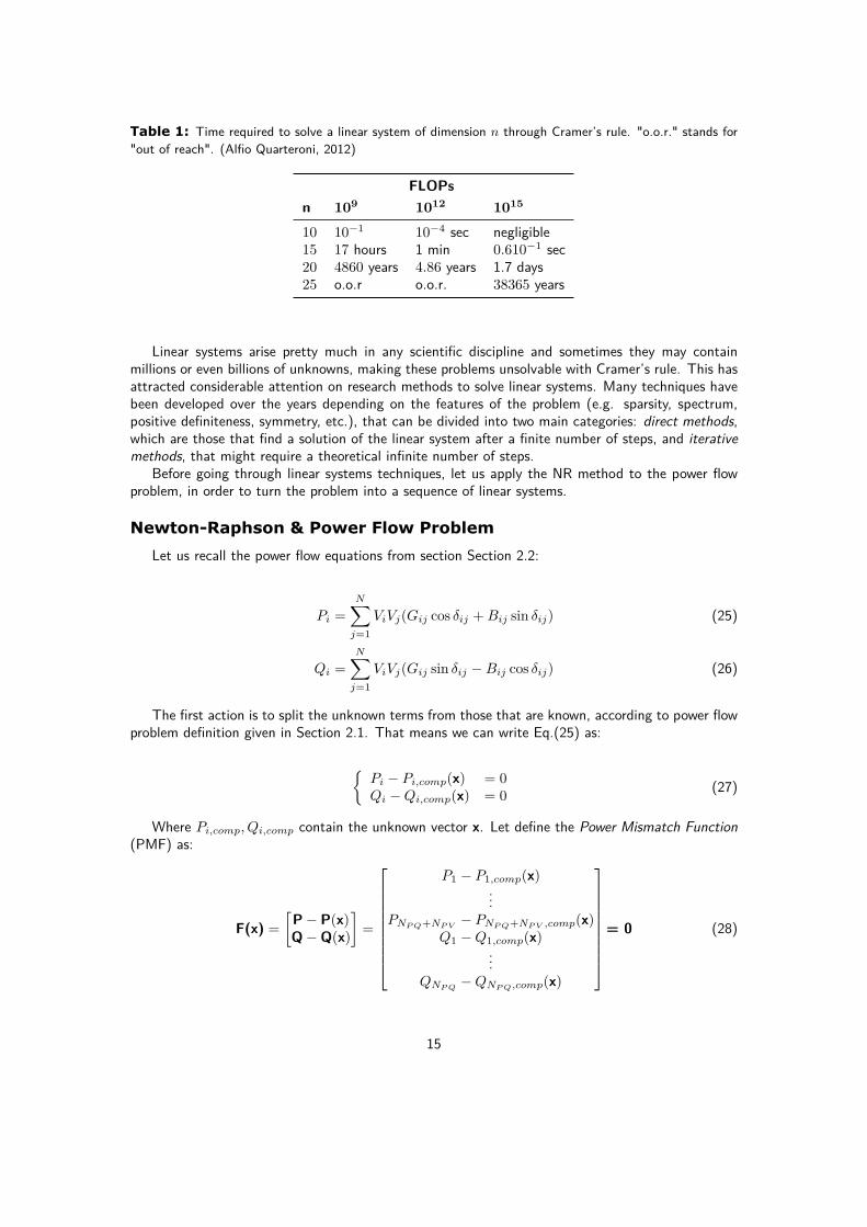
Table 1: Time required to solve a linear system of dimension n through Cramer’s rule. "o.o.r." stands for"out of reach". (Alfio Quarteroni, 2012)
FLOPsn 109 1012 1015
10 10−1 10−4 sec negligible15 17 hours 1 min 0.610−1 sec20 4860 years 4.86 years 1.7 days25 o.o.r o.o.r. 38365 years
Linear systems arise pretty much in any scientific discipline and sometimes they may containmillions or even billions of unknowns, making these problems unsolvable with Cramer’s rule. This hasattracted considerable attention on research methods to solve linear systems. Many techniques havebeen developed over the years depending on the features of the problem (e.g. sparsity, spectrum,positive definiteness, symmetry, etc.), that can be divided into two main categories: direct methods,which are those that find a solution of the linear system after a finite number of steps, and iterativemethods, that might require a theoretical infinite number of steps.
Before going through linear systems techniques, let us apply the NR method to the power flowproblem, in order to turn the problem into a sequence of linear systems.
Newton-Raphson & Power Flow Problem
Let us recall the power flow equations from section Section 2.2:
Pi =N∑j=1
ViVj(Gij cos δij +Bij sin δij) (25)
Qi =N∑j=1
ViVj(Gij sin δij −Bij cos δij) (26)
The first action is to split the unknown terms from those that are known, according to power flowproblem definition given in Section 2.1. That means we can write Eq.(25) as:
Pi − Pi,comp(x) = 0Qi −Qi,comp(x) = 0 (27)
Where Pi,comp, Qi,comp contain the unknown vector x. Let define the Power Mismatch Function(PMF) as:
F(x) =[P− P(x)Q−Q(x)
]=
P1 − P1,comp(x)...
PNP Q+NP V− PNP Q+NP V ,comp(x)
Q1 −Q1,comp(x)...
QNP Q−QNP Q,comp(x)
= 0 (28)
15

The PMF represents the system of non-linear equations in a compact form. From the PMFside, the power flow problem consists in determining the vector of state variables x so that the netinjections/withdrawals Pi, Qi equal those computed from state variables.
As mentioned in the previous section, the NR procedure starts with the linearisation of the initialproblem. This gives:
F(x) =
P1 − P1(x(k+1))P2 − P2(x(k+1))
...Pn − Pn(x(k+1))Q1 −Q1(x(k+1))Q2 −Q2(x(k+1))
...Qm −Qm(x(k+1))
≈
P1 − P1(x(k)) + ∇P1(x(k)) ·∆x(k) = 0P2 − P2(x(k)) + ∇P2(x(k)) ·∆x(k) = 0
......
...Pn − Pn(x(k)) + ∇Pn(x(k)) ·∆x(k) = 0Q1 −Q1(x(k)) + ∇Q1(x(k)) ·∆x(k) = 0Q2 −Q2(x(k)) + ∇Q2(x(k)) ·∆x(k) = 0
......
...Qm −Qm(x(k)) + ∇Qm(x(k)) ·∆x(k) = 0
(29)
With n = NPQ + NPV and m = NPQ. Exactly as before, the gradient terms are all vectors,so that they can be gathered into a matrix of dimension (n + m)x(n + m). We call this matrix theJacobian matrix of the power flow problem JPF . Reordering, the non-linear problem is turned into asequence of linear systems k as:
−J(x(k))∆x(k) = F(x(k)) (30)
With the unknown vector defined as:
x =[Vδ
]=
V1...
VNP Q
δ1...
δNP Q+NP V
(31)
Note that JPF has a block structure. By dividing the derivatives of P,Q with respect V, δ, werecognise a structure made up of four blocks:
JPF =
∂P(x)∂δ
∂P(x)∂V
∂Q(x)∂δ
∂Q(x)∂V
(32)
For sake of simplicity from now on we refer to JPF as J . An example of the Jacobian structure isreported in Fig. 3 (case13), to underline its block structure. This case has been created by mergingcase9 and case5 of Matpower libraries (Zimmerman and Murillo-Sanchez, 2016).
It is worth reporting that most power flow software set up the reduced Jacobian, meaning thatrows related to slack and PV reactive power equations are not included. For this reason, the Jacobianfor case13.m has size 19x19, rather than 26x26. From now on we will use the term reduced Jacobianto indicate the first case and the term full Jacobian to indicate the latter.Note that the Jacobian structure might differ from case to case, depending on the implementation.PETSc follows a different rational indeed. The derivatives ordering follows a bus ordering. As a
16
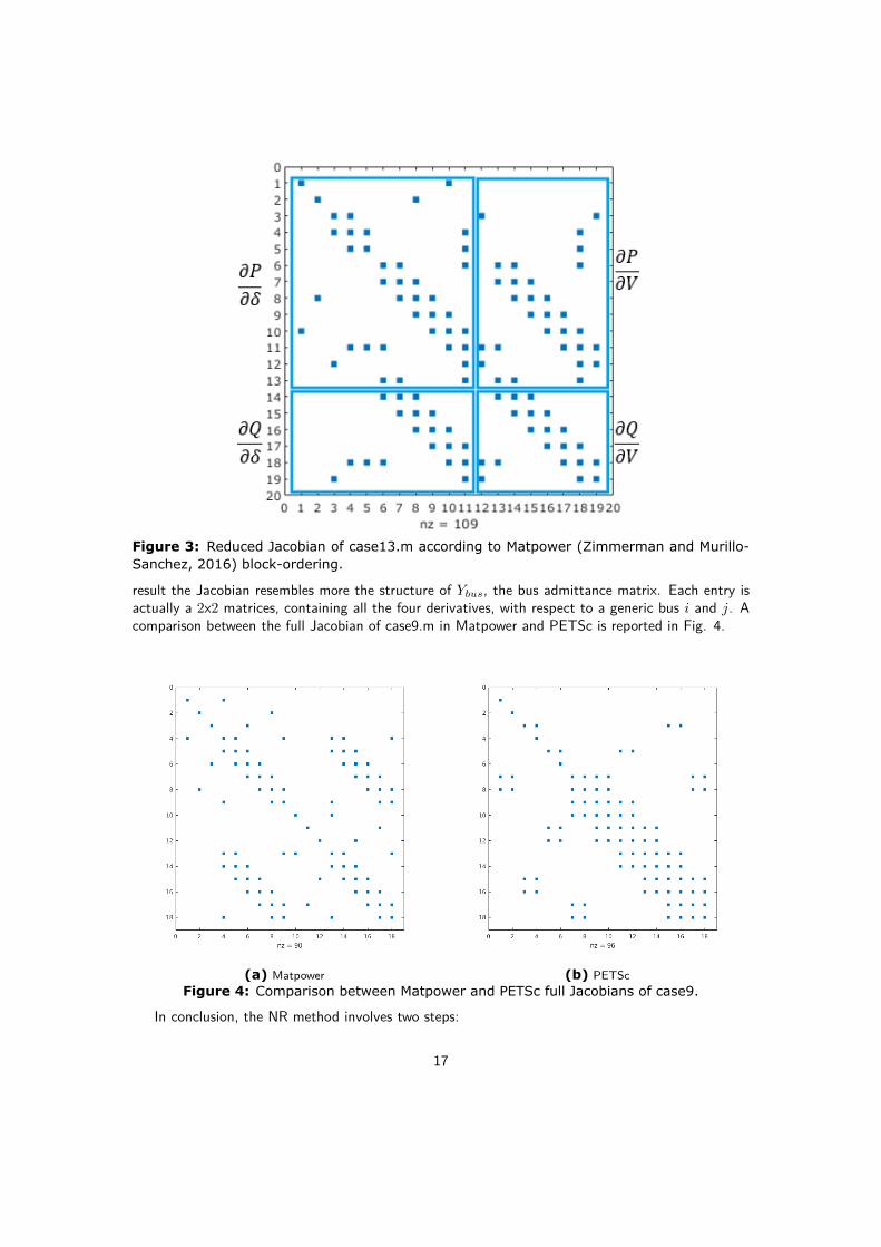
Figure 3: Reduced Jacobian of case13.m according to Matpower (Zimmerman and Murillo-Sanchez, 2016) block-ordering.
result the Jacobian resembles more the structure of Ybus, the bus admittance matrix. Each entry isactually a 2x2 matrices, containing all the four derivatives, with respect to a generic bus i and j. Acomparison between the full Jacobian of case9.m in Matpower and PETSc is reported in Fig. 4.
(a) Matpower (b) PETScFigure 4: Comparison between Matpower and PETSc full Jacobians of case9.
In conclusion, the NR method involves two steps:
17

1. Solve J(x(k))∆x(k) = −F (x(k))
2. Update x(k+1) = x(k) + ∆x(k)
Note that when using an iterative linear solver, step 1) of the procedure should be better called:’solve approximately J(x(k))∆x(k) = −F (x(k))’ due to the fact that iterative solvers solve the Ja-cobian linear system up to a given a tolerance. This class of methods are called Inexact-Newtonmethods and are the main matter of this work. In the next sections aspects regarding linear solverswill be dealt in detail. Note that proper tolerances shall be used for the linear (Krylov-Schwarz)iterations: in fact, while an excessive rough solution could lead to an increase of non linear iterations,an excessive precise solution would lead to a waste of computational resources.
2.3.2 Newton-Raphson with Line Search
The NR method presented in the previous sections is a basic but effective approach to solvenon-linear problems. The NR converges quadratically, which is good, though may not be robustenough for real applications. In commercial applications, the NR method is implemented with somemodifications to improve convergence properties. The two main techniques are that of the trust-regions and the line-search technique, more common in the context of power flow equations. Herewe briefly recall the idea.
Let consider the non-linear update scheme derived in the previous section:
x(k+1) = x(k) + ∆x(k), −J(x(k))∆x(k) = F(x(k)) (33)
In this expression the updating vector ∆x(k) can be interpreted as a correction vector, giving thenew direction x(k+1). In principle we expect ∆x(k) to be decreasing over the non-linear iterations,reaching out the zero value when the exact (up to an accepted tolerance) solution is found. Thiscould not be the case for any iteration k and the procedure may even diverge. The line-search makesthe NR procedure converging for any starting guess x(0). When this happens we say NR is globallyconvergent12. The idea of line-search is quite simple. We introduce a parameter σ in the updatingscheme according to:
x(k+1) = x(k) + σ(k)∆x(k) (34)
And set σ(k) as the term which minimises:
argminσ
∥∥∥F (xk − σ(k)∆x(k))∥∥∥ (35)
This minimisation problem cannot be solved analytically, but usually an approximated solution isenough to provide the desired result. For more information about line-search and trust region seefor instance (Idema and Lahaye, 2014). This approach belongs to the broader category of gradientmethods. This will be important in the context of non-stationary iterative linear solvers, that will bethe main matter of the next sections.
12Note that this ensures global convergence at local minimum. Which means, in general to the closer solution tox(0). This shall be strongly taken in mind when interpreting the results.
18

2.4 Introduction to Linear Solvers
One of the most well-known scopes of computer science is to study algorithms that can ease thesolution of complex computational problems. Among the many features that an algorithm shouldhave there are indeed efficiency, elegance and stability. In other words, algorithms shall make minimaluse of computational resources, shall be easy to be read and implemented, and shall not magnifynumerical errors, potentially induced by particular sets of inputs. While a comprehensive discussionis out of the scope of the present work, a short overview of some notable techniques will be providedto better motivate the linear solver discussion for distributed power flow.
As mentioned in Section 2.3, linear solvers are divided into direct and iterative. The two approachesdiffer in the formulation as well as in their distinctive features. For instance, one of the most relevantcharacteristic of direct solvers is their robustness. This has lead direct methods to be preferred overiterative in the industry practice, as the property of giving reliable solutions on different sets of inputsis of key importance. On the other hand, iterative methods are mostly still used in research contexts,as they can perform much better when problems scale up.
Remarkably, the reason behind using iterative linear methods in this work is not strictly the speed-up to find the solution of the power flow problem, rather than its parallel features that perfectly fitthe scope of a distributed computation. This will gradually become clearer. Here, we start briefly byintroducing the general formulation of direct and iterative methods. After that, we will introduce theiterative solver actually used and discuss it in detail.
2.4.1 Direct Methods
Let A be the coefficient matrix and b the right-hand side of the linear system:
Ax = b (36)
The solution of the unknown vector x is approached by direct methods by factorising the coefficientmatrix A into a product of two matrices M,N that gives back A, so that Eq.(36) can be re-writtenas:
MNx = b (37)
Once the M,N matrices are found, the solution of Eq.(36) is easily found. In practice, the maineffort of the direct methods is on the factorisation of the A matrix. A prominent example of directmethod is the LU factorisation method, which factorises A into a lower triangular matrix L and anupper triangular matrix U . In practice, the L,U matrices are based on the the Gaussian elimination,a well-known algorithm proposed by Gauss in the ’800s. The Gaussian elimination process may failin some occasions. In order to avoid such occurrences, A rows and columns are permuted beforefactorisation. This procedure is called total pivoting and allows to get to an important result: givenany non-singular coefficient matrix A, it is always possible to find a permutation of its columns androws so that Gaussian elimination is possible: it is always possible to find the matrices L,U . This factgives an immediate proof of the robustness of direct methods. On the other hand, direct methodssuffer from the so-called fill-in process. In practice, it is quite common to deal with sparse linearsystems13; this is usually an advantage, as it lowers the memory storage and simplifies the coupling ofequations in the system. The fill-in phenomena occurs during the factorisation process which inducea lot of non-zero elements to show up.
13In numerical analysis a sparse system is a matrix in which most of the elements are equal to zero.
19

2.4.2 Iterative Methods & Preconditioning
Iterative methods seek for the solution of Eq.(36) through consecutive refinements of approximatesolutions. A common procedure is to find the generic iterate x(k+1) by means of a fixed point iterationscheme, that means through the general:
x(k+1) = Φ(x(k)) (38)Most of the iterative schemes in the literature are based on a linear map Φ. This represents
a simple basis for analysis of the properties of the iterative scheme, without actually precluding itsefficiency. More complex features can be added, but also in these cases the updating scheme is stilllinear. A linear iterative scheme updates the solution through:
x(k+1) = Bx(k) + f (39)Where B, f are respectively the iteration matrix and a vector, both function of A,b. In principle,
iterative schemes converge to the exact solution x∗ = A−1b only after an infinite number of iterations.In practice this is not possible nor actually needed. Let us introduce the error e = xk − x∗ relative tothe step k as the vector depicting the ’distance’ from the exact solution. What would be sufficient isto stop the iteration process after the iteration k that makes the error norm small enough:∥∥∥e(k)
∥∥∥ =∥∥∥x∗ − x(k)
∥∥∥ < ε (40)
That is, lower than a certain quantity ε. Of course, the error is an unknown quantity and canonly by estimated at each iteration k. In practice we use an estimator of the error and we check itsvalue against our tolerance ε. The most common estimator used is the residual, as it is often alreadyavailable during the iteration process. We define the residual r as:
r = b−Ax (41)And do at each iteration k a check on its norm. The check may involve both the residual norm
relative to the right hand side vector b and its absolute norm.Note that the residual expression equals zero for the exact solution x∗, exactly as it does the error
expression (Eq.(40)). This might give the wrong idea that the residual perfectly estimates the error.Actually, as the machine can only approximate real numbers to floating point numbers, errors areconstantly introduced in the iteration process acting as perturbations and eventually leading to falsesolutions. In other words, we may find a solution that respects our residual tolerance conditions:
‖r‖ < ε1 and‖r‖‖b‖
< ε2 (42)
While actually being far from the exact solution x∗. Linking the error norm and the residualnorm is not an easy task. It depends on many factors, among which the coefficient matrix A relatedproperties (e.g. symmetry or positive definiteness), on the numerical perturbation considered, onthe iterative scheme, on the norm definitions, etc. Generally, is common to find expressions thatrelate the error norm to the residual norm through the so-called condition number K(A), which asstated in the notation is strictly dependent on the coefficient matrix. For instance, if we considerA symmetric and positive definite (SPD) and we consider numerical perturbations only on the righthand side vector b, the error norm relates to the residual norm at the generic step k through thefollowing expression: ∥∥x(k) − x∗
∥∥∥∥x(k)∥∥ ≤
∥∥r(k)∥∥
‖b‖ (43)
20
With the condition number being equal to:
K(A) = λmaxλmin
(44)
In general, we can consider the condition number as a measure of how much we expect the errorto be small with respect to the residual. The greater the condition number K(A), the greater thedifference between the residual and the error. This introduces us to the concept of preconditioning.Preconditioning is a widely used technique aiming at facilitating the iterative process by diminishingthe condition number, in other words, to diminish the impact and propagation of numerical errors.Actually, any linear system that has lower condition number is in turn easier to solve, therefore wecan say that preconditioning helps in general the solution finding process.
Convergence Analysis
Convergence is an important, if not the most important, feature of numerical methods. Whenbuilding an iterative scheme, for instance taking into account Eq.(39), two of the most importantthings that we would like to know are:
• Does Eq.(39) converge to the exact solution?
• How quick does the Eq.(39) converge?
To answer these questions we need to derive some properties of the iteration matrix B. In order forthe Eq.(39) to converge to the exact solution, it is necessary that the following consistency conditionis fulfilled:
x∗ = Bx∗ + f (45)(46)
In other words, if we let B to be freely chosen, we are obliged to set f in order to respect theequality above. Let us now subtract the Eq.(45) from Eq.(39) so that we obtain a recursive expressionfor the error:
e(k+1) = Be(k) (47)As any iterative procedure starts with a first guess x(0), we can also write:
e(k) = Bke(0) (48)This gives a clear insight on the role of B: the method converges if and only if B acts as a
diminishing factor for the error through iterations. The iteration matrix is the parameter we act onto design the iterative method according to our needs, as it gives all the convergence properties ofthe iterates. We can write a more formal convergence criterion by using eigenvalues and eigenvectorproperties. Recall that, given λ ∈ Rn as a scalar, an eigenvector w of B is any vector for which thefollowing equality holds:
Bw = λw (49)The λp is called an eigenvalue of B. Let us assume that B has a complete set of eigenvectors
(for instance this occurs when B is SPD)14. This means, given n as the matrix order of B, we have14The result that we will get here can be extended also in the case B does not have a full set of eigenvectors. This
is not treated here, but can be found for instance in (Saad, 2003) at section 4.2.1.
21
a set w1,w2, . . . ,wn independent vectors that form a basis ∈ Rn. As n is also the order of e(0), wecan write e(0) down as a linear combination of the eigenvectors w1,w2, . . . ,wn:
e(0) = c1w1, c2w2, . . . , cnwn (50)
With c1, c2, . . . , cn being a unique set of coefficients. Combining Eq.(48), Eq.(49) and Eq.(50)we get:
e(k) = c1λk1w1 + c2λ
k2w2 + · · ·+ cnλ
knwn
k → inf≈ max
p∈1,...,n|λp|k (51)
Which approximates to the term containing the greater eigenvalue in module as k → inf. Wedefine this term as the spectral radius of B. Explicitly this means:
ρ(B) , maxλp∈λ1,...,λn
|λp| (52)
Finally, the expression for e(k) becomes:
e(k) ≈ ρ(B)k (53)
And hence it is a necessary and sufficient condition for the convergence that ρ(B) < 1. Further-more, the lower the spectral radius the quicker the convergence.
Basic Iterative Methods
Here we want to derive explicitly some basic iterative schemes. A common way to derive aniterative scheme is through the splitting of the coefficient matrix A. In other words we write A as:
A = M −N (54)
With M necessarily a non-singular matrix. Substituting into Ax = b we get:
x(k+1) = M−1Nx(k) +M−1b (55)
The matrix M is called preconditioning matrix. Recalling Eq.(39), the iteration matrix B is nowdefined as:
B = M−1N (56)
Which suggests that the preconditioning matrix actually influences the convergence properties ofthe iterates. A further rework can be done on Eq.(55) in order to get an expression of B as a functiononly of M and A. Let us set:
N = M −A (57)
Eq.(55) can be written as:
x(k+1) = (I −M−1A)x(k) +M−1b (58)
Which, by comparison with Eq.(39) gives the expression of the iteration matrix:
B = I −M−1A (59)
22

As the spectral radius of B gives the convergence rate, the iterative method converges fast in thecase we make:
ρ(B) = ρ(I −M−1A)→ 0 (60)This happens in the case M ≈ A15. Of course, the extreme case M = A is meaningless since we
are inverting A itself and the preconditioning is of no help. In contrast, taking M very different fromA may lead to spectral radius values just slightly lower than one, making the convergence very slow.This gives us an important insight: it is important to find the right balance between the applicationcost of the preconditioner and the actual ease gained from its introduction, i.e. in terms of spectralradius.
This highlights another important fact. Direct and iterative methods are not that far as it mayseems, in practice the insights from one are combined into the other. One can make use effectively ofa direct technique to build a preconditioner. Many recipes can be designed in this sense, for instanceone may carry out an incomplete factorisation of A in order to have A ≈ LU , set M = LU anditerate through Eq.(58). By this approach, as M ≈ A, we can obtain convergence in few iterations,while saving at the same time computational resources from a full factorisation.
Preconditioning Formulations
Splitting is just one of the methods to derive an iterative scheme. Depending on the idea aswell as on the needs of the iterative solver, one can define the application of the preconditionerthrough alternative formulations. An example is to transform the linear system Ax = b into theleft-preconditioned:
M−1Ax = M−1b (61)Alternative preconditioning formulations may be based on right-preconditioning :
AM−1y = b, x = M−1y (62)Or split-preconditioning. Assume to have M in a factorised form, that means M = MLMR. The
split-preconditioning formulation modify Ax = b as:
M−1AMy = M−1b, y = M−1x (63)Split-preconditioning is often used when we want to preserve the symmetry of the problem. For
instance, consider having M in the form:
M = CCT (64)The split-preconditioned linear system:
M−1AMy = M−1b, y = M−1x (65)Is always symmetric.Right-preconditioning can be used to preserve the residual expression, that can be advantageous
for some algorithms for residual check, whereas left-preconditioning uses the preconditioned residual:
z = M−1r = M−1(b−Ax) (66)Through iterations. In conclusion, preconditioning shall be applied by following the two-step
procedure:15In fact: M ≈ A means the product M−1A ≈ I, hence ρ(B) ≈ 0
23

1. Select a preconditionerM that is easy to build and ensure an easy solution of the preconditionedlinear system Mz = r.
2. Choose the preconditioning formulation that is the most tailored to the application, propertiesof the coefficient matrix A (e.g. symmetry), etc.
For more details on preconditioning formulations see (Ferronato, 2012).Note that we can easily show that Eq.(61) is totally equivalent to a Eq.(39). Let us recall Eq.(58).
This must necessarily holds also for the exact solution x∗, that means one can write it down also as:
x∗ = (I −M−1A)x∗ +M−1b (67)
Gathering the terms in x∗ the Eq.(61) is obtained. In general, regardless of the preconditioningformulation that we use, we can always lead back to an update scheme of the kind of Eq.(39) andanalyse the convergence characteristics by identifying the expression of the matrix B. For right-preconditioning this can be done as:
AM−1y = b (68)AM−1y + y− y = b
y(k+1) = (I −AM−1)y(k) + b
Which gives an expression for B almost16 identical to that of left-preconditioning. The lastequation above can be also written as:
y(k+1) = y(k) + b−AM−1y(k) (69)Mx(k+1) = Mx(k) + r(k)
Which shows how the right-preconditioning formulation preserves the residual expression.An interesting question may arise on preconditioning formulations. Does the spectrum of B
changes when applying the three different expressions of preconditioning? It can be proved (see(Saad, 2003)) that the spectrum of Eq.(61), Eq.(62) and Eq.(63) is equal and hence one shouldnot expect different convergence properties. This is actually verified only in exact arithmetic. Asproblems are more ill-conditioned, in practice we can have different performances depending uponthe preconditioning formulation chosen. For instance, if A resembles a symmetric matrix the split-preconditioning may be the preferred formulation.
2.4.3 Practical Updating Schemes & Basic Implementation Algo-rithms
The expressions derived so far about the iteration matrix B are fundamental for convergenceanalysis and to the understanding of the properties of an iterative method. However they are nottailored for implementation schemes. Here we want to introduce expressions that can be used forimplementations. Let us start by reworking a bit the following equations:
16The matrix-matrix product is not commutative. This means in general AM−1 and M−1A differ with each other.
24

x(k+1) = M−1(M −A)x(k) +M−1b (70)= (I −M−1A)x(k) +M−1b= x(k) +M−1(b−Ax)= x(k) +M−1r(k)
This gives an updating scheme for x(k) that only involves the residual and the preconditioner. Letdefine z(k) = M−1r(k), conceptually the Eq.(70) consists of three steps: solving the preconditionedlinear system in z(k), update the solution and update the residual for the next iteration. A pseudo-algorithm for a stationary iterative method can be thus:
Algorithm 1 Prototype algorithm for stationary iterative linear solver.1: Begin2: initialize x0, r0 = b−Ax03: for k = 0, 1, . . . , until convergence do4: solve Mz(k) = r(k)
5: update the solution x(k+1) = x(k) + z(k)
6: update the residual r(k+1) = r−Ax(k+1)
7: end for8: End
An alternative way of updating the residual is sometimes used:
r(k+1) = b−Ax(k+1) (71)= b−A(x(k) + z(k))= r−Az(k)
From the computational point of view this costs one matrix-vector multiplication exactly as for theprevious update scheme. In more complex iterative schemes, algorithms involve much more steps andthe product Az(k) might be already available at the residual update step, making it less expensive.
The algorithm shows us another important thing. At each step k we solve the preconditionedlinear systemMz(k) = r(k). Again: the closerM ≈ A, the higher the computational cost per iterationwill be. Whereas taking M such that it is easier to solve Mz = r means in general to produce moreiterations k before convergence is reached. Generally, the preconditioning matrix M is chosen so thatit balances the computational cost per iteration k and the ease to obtain the solution of the linearsystem. In practice, the design of a proper preconditioner is a complex task and should take intoaccount many factors, such as the physics of the problem or the sparsity of the coefficient matrix A,and depend upon the specific needs of the iterative solver (i.e. decrease computational complexityof the problem, provide numerical stability, enhance condition number of the problem, etc.). For amore detailed discussion on preconditioning see (Chen, 2005), (Saad, 2003), (Benzi, 2002). In thecontext in exam, it is sufficient to consider the preconditioner as a ’facilitator’ for the convergence ofthe succession Eq.(39), though, as it will be discussed in Section 2.5, it must fulfil other additionalrequirements.
25

Non-Stationary Iterative Methods
So far the preconditioning theory has taught us to build an iterative method and to make analysison its convergence. The basic schemes seen belong tothe family of the stationary iterative methods.The term stationary is quite straightforward: the Eq.(70) does not change through the iterations.However, these schemes are not tailored for real applications as soon as the number of iterations grows,which is the case of many real problems. To this aim the concept of dynamic iterative methods needsto be introduced. These methods make use of some parameters that are optimally chosen at eachstep k to speed up the convergence.
More formally, let us introduce the scalar α 6= 0 ∈ R and modify Eq.(70) as follows:
x(k+1) = x(k) + αz(k) (72)
Which can also be written as:
x(k+1) = (I − αM−1A)x(k) + z(k) (73)
Due to the introduction of α, the spectral radius is changed into:
ρ(B) = ρ(I − αM−1A) (74)
As known, the lower the spectral radius the faster the convergence is reached. The followingminimisation problem can hence be set:
minαρ(I − αM−1A) (75)
To find an optimal value for α. This simple iterative scheme is known as Richardson’s iteration.It is possible to do even better by allowing α to change at each iteration k, meaning that α isdynamically updated through the iterations k. From now on we will denote α as α(k) every time weintend it as a dynamic parameter. This introduces us to the gradient method. The gradient methodcomputes α(k) in order to obtain the minimal value for the norm of the residual vector at iterationk + 1. In short, it sets at each iteration k the minimisation:
minα
∥∥∥x(k) + α(k)r(k)∥∥∥ (76)
Empirically, among all the linear vectors x(k) +α(k)r(k) we are looking for the optimal step lengthα(k) that makes the next residual minimal. In this conception the residual vector is interpreted asthe search direction along which we move in order to find the next iterate x(k+1). This schemecan be further improved by choosing alternative directions to the one given by the residual vector.The conjugate gradient (CG) algorithm, for instance, takes conjugate (i.e. orthogonal) directions toupdate the iterate according to the following:
x(k+1) = x(k) + α(k)p(k) (77)
Further insights can be gained by expanding between the first iteration (0) and the generic iteration(k). This gives:
x(k) = x(0) + α(1)p(1) + α(2)p(2) + · · ·+ α(k−1)p(k−1) = x(0) + δ (78)
Basically, we are looking for a correction vector δ which is the linear combination of the set ofvectors p(1),p(2), . . . ,p(k−1). Since these vectors are all conjugate between each other, they forma basis for a subspace of dimension equal to k − 1. One could think that as k gets to n − 1, theconstructed basis can be used to describe any vector of dimension n, including the solution vector.
26

This is not completely true, as generic n-dimensional vectors could lie in different spaces. In otherwords, constructing such a basis is not in general an easy task. For SPD coefficient matrix A we canprove that CG can find the exact solution in such space by minimsing the error in the A-induced norm.In other words, the CG method converge in exactly n iterations, other than numerical errors. For thisreason sometimes the CG method is considered a direct method. For a more in-depth derivation ofthe conjugate gradient method and mathematical proofs of the concepts presented, see for instance(Gutknecht, 2007).
In practice, dynamic schemes are always used with proper preconditioners. In other words, we caninterpret dynamic schemes as accelerators for the previously introduced stationary schemes. Noticethat one can decide to solve the linear system only by means of an accelerator (i.e. without anypreconditioner, that means setting M = I) or only by means of a stationary iterative scheme (i.e.without any accelerator, that means with α(k) = 1 and update direction given by r(k)). Even thoughwhen such techniques are combined together give definitely better performances. Another possiblechoice is the ’order’ of the preconditioner-accelerator. In this sense we distinguish preconditionedaccelerators and outer-inner dynamic schemes. In other words, we can either left-precondition thelinear system through:
M−1Ax = M−1b (79)
And apply an accelerator, getting an update scheme as:
x(k+1) = x(k) + α(k)M−1p(k) (80)
Or use the right-preconditioning to obtain an outer-inner scheme that employ the preconditioneras an inner iteration inside the accelerator. In this configuration some notable mentions go to theouter-inner Krylov solvers and flexible preconditioned Krylov methods. Outer-inner Krylov solversemploy a double Krylov Subspace procedure, one for the outer iteration and one as a preconditioner,which means to solve the preconditioned linear system. On the other hand, flexible preconditioningallow to change the preconditioner inside Krylov iterations.
Krylov Subspace Projection Methods
In this section we further generalize the idea of dynamic iterative methods by introducing Krylovmethods. Preconditioned Krylov methods are among the more effective iterative techniques to solvebig sparse linear systems. The CG method is for instance part of this large classes of iterative methods.Despite CG is considered to be the best method to solve symmetric positive-definite (SPD) problems,Krylov methods offer efficient approaches also for non-SPD problems. In our context, the Jacobianof the power flow problem is not symmetric17. For this reason, more ’general’ Krylov methods shallbe employed, as the Generalized Minimal REsidual (GMREs) method(Saad and Schultz, 1986). Inthis section we want to introduce the Krylov methods and present some of their key features.
A Krylov Projection Subspace can be defined in many ways. A common definition for KrylovSubspace is the following. Consider a generic n × n matrix A and a n × 1 vector c, we define theKrylov Subspace K generated by the matrix-vector multiplications of (A, c) as any space constructedas follows:
Kv(A, c) , c, Ac, . . . , Av−1c (81)
In general, the sequence c, Ac, . . . , Av−1c does not yield a linear independent sequence of vectors,meaning that dimKv ≤ v. How such a sequence can be used to solve a linear system? Say that
17This can be easily noticed by looking at the block structure of the Jacobian Eq.(32). Derivatives in block 1,2 andblock 2,1 are different, hence the matrix is generally not symmetric.
27
A is the space spanned by the columns of A and c is a generic n × 1 vector. As we consider onlywell-posed problems having det(A) 6= 0, the dimension of A is exactly n. The idea behind Krylovmethods is to extract a subspace K ⊆ A having a dimension v << n so that we can find inside it a’sufficient good’ solution. More precisely we look for the approximate solution xv in the affine spacex0 +Kv(A, c) which has the form:
xv = x0 + δ = x0 + Vvyv (82)
If xv lies in the affine space, and the dimension v of Kv(A, c) is small, we can compute xv easily.Notice that the correction vector δ (previously introduced in Eq.(78)) is expressed through the linearcombination Vv, yv, which indicate the matrix for the basis of the Krylov Subspace and a propervector of coefficients respectively. In general Krylov methods differ among themselves in the mannerthe basis are built and the weights yv are computed.
The GMREs (Generalized Minimal REsidual) method solve a linear system Ax = b by setting upthe following minimisation problem:
miny∈K(A,b)
‖b−Ax‖ (83)
In other words, GMREs looks for the vector yv that, among all the vectors in K(A,b), gives backthe minimal residual vector. In order to solve the minimisation problem we need a tailored basis forthe Krylov Subspace. This could be done by constructing the sequence:
Kv(A, r(0)) = r(0), Ar(0), . . . , Av−1r(0) (84)
As mentioned this is actually not a basis, as such vectors are linear dependent. In principle, wecould stop the matrix-vector multiplications as v gives the first dependent vector. In practice this isnot done as the sequence is poorly linear independent, leading to an ill-conditioned basis that is notsuitable for use. For this reason some ortho-normalisation process must be employed. The GMREsmakes use of a modified version of the Gram-Schmidt ortho-normalisation (i.e. the Arnoldi process)in order to obtain the Krylov basis. The GMREs algorithm can be outlined in three conceptual steps:
1. Ortho-normalise the sequence r(0), Ar(0), . . . , Av−1r(0) to create the Krylov basis Vv;
2. Solve the residual minimisation problem to compute yv;
3. Update the solution with Eq.(82).
The computational cost of the first step scales up much faster than linearly as the dimension ofthe Krylov Subspace increases. For this reason a fourth step is usually added to the procedure above.This sets the possibility to restart the procedure after some dimension v of the subspace is reached.This modification consist in the Restarted-GMREs (R-GMREs) version of the algorithm. The R-GMREs starts back the procedure in the case the solution obtained does not fulfil the estabklishedtolerance. If such situation occurs, R-GMREs takes as the first iterate the solution obtained by theprevious subspace, setting then x(0) = x(v).
2.4.4 Computational Complexity of Direct and Iterative Methods
Computational complexity can be retained as the amount of computational resources needed tosolve a computational problem. An important step when solving scientific computing problems is toassess the computational complexity of the problem in exam. In turn, algorithms are chosen in orderto decrease the amount of resources required to solve the problem. Usually, two main resources are
28
considered: the computational space i.e. memory requirements and computational time i.e. the timerequired to solve a given computational problem.
In this section we want to give a short insight on the computational complexity of direct anditerative methods as a function of the size and scale of the problem. This will help us later inidentifying the main ’computational features’ of the power flow problem. We find the FLOPs (floatingpoint operations) required for a direct and an iterative solver for a dense18 linear system as functionof the dimension n of the linear system and draw some straight conclusion.
Let’s start considering the LU method. The LU method looks for a factorisation of A in a lowertriangular matrix L and an upper triangular matrix U , so that a linear system Ax = b is turned intothe two equivalent linear systems:
Ly = b, Ux = y (85)
Once L and U are found, the solution of the two systems above can be easily found. The triangularstructures of L and U gives a series of equations totally decoupled. For instance, consider the systemLy = b. The first equation contains only the first unknown, the second equation contains only thefirst and second unknown, hence is only function of the first, the third is only function of the firsttwos, etc. In other words, we can solve the two triangular linear systems above through backward (U)and forward (L) substitution. From the computational point of view this costs only n2−n operations.The expensive stage is the factorisation process. Let’s consider the Gaussian elimination algorithmas the process to find the matrices L and U . This algorithm costs roughly 2/3n3. A proof for thiscan be found for instance in (Farebrother, 1988). As n gets sufficiently large, the computationalcomplexity of a direct method for dense matrices can be approximated to O(n3).
An iterative method updates the solution through the standard linear fixed point iteration scheme(Eq.(39)). This costs at each iteration k at least one MVM: which means n ∗ (n + (n − 1)) =2n2 − n operations plus, at least, 2n summation operations to update the solution and residual withf. Basically this means that an iterative method cost is in the order of O(kn2). This allows us todraw some simple conclusions. Suppose the iterative method converges (i.e. iterations usually are< 100000), problems that scale up over 105 unknowns give a computational advantage to iterativemethods compared to direct methods. In practice, iterative methods are not implemented accordingto Eq.(39), though the computational expenditure can still be approximated to the matrix-vectormultiplication only.
Assessing in detail the actual computational complexity of an algorithm is not an easy task andit is a study subject by itself, as many other factors come into play (e.g. matrix-vector specificimplementations, sparsity, parallelism, ecc.). In the next sections to provide a more comprehensiveview to the reader we discuss (qualitatively) the role of sparsity and parallelism to assess computationalcomplexity.
Sparsity
Let us now introduce the concept of sparsity19. When dealing with sparse matrices the compu-tational complexity becomes of the order of O(nz), where nz is the number of non-zero entries ofthe coefficient matrix. This represents a further advantage for iterative methods for at least tworeasons. First, direct methods use factorisation processes that lead the initial sparse matrix to befilled-in. The higher the number of non zero-entries of LU matrices, the greater the computationalcomplexity, meaning that more memory storage is required as well as more operations to solve thelinear system. The second reason being that in general it is more difficult to develop factorisation
18The matrix A which describes the system has only non-zero entries.19There is not strict definition of sparsity of a matrix. Simply speaking, a sparse matrix is a matrix whose entries
are mostly zero elements.
29

algorithms that take fully advantage of zero entries. In practice, sparsity is one of the reason whyiterative methods perform better for solving large sparse linear systems.
Parallelism
When dealing with complex scientific problems, solving algorithms are designed to efficiently runin parallel on dedicated computing platforms (e.g. clusters). The benefits from parallelising the sourcecode in which the algorithm are written are usually measured by comparing the simulation sequentialtime with the simulation parallel time. To this aim the speed-up factor S is defined as:
S = sequential computational time [s]parallel computational time[s] (86)
The program has linear speed-up if S = p where p is the number of cores used in the executingprogram. Efficiency is said to be the ratio between speed-up and the number of cores used in thecomputation E = S/p. In practice, E is always less than one, mainly for two reasons. First, problemscannot be completely broken down into sub-tasks, that is, cannot be fully parallelised. For instance,from Amdhal’s law one can see that even in the favourable case of a 90% of code parallelisable themaximum theoretical speed-up can be equal to 10. The second reason is that processors need tocommunicate with each other when sub-tasks are coupled. Let us consider a simple example to clarifythis last point.
Example 1. Let us consider the dot-product operation of two Rn vectors v and w. The result λ ofthe dot-product is a scalar given by the following operation:
λ = 〈v,w〉2 = vTw =n∑i=1
viwi = v1w1 + v2w2 + · · ·+ vnwn
How can we parallelise such an operation? Let consider two processors p1 and p2. We can splitequally the number of n products and the n − 1 summations over the two processors. This meansp1 does:
λ1 = v1w1 + v2w2 + · · ·+ vmwm
And p2 does:λ2 = vm+1wm+1 + vm+2wm+2 + · · ·+ vnwn
In order to compute λ we need to add up the two contributions e.g. send λ2 from p2 and makep1 ready to receive it. This means we need a global communication operation. The send andreceive operations are message passing primitives and are at the basis of inter-process communica-tion protocols (IPCs).
Eventually, one processor computes:
λ = λ1 + λ2
This simple example shows us two things:
1. We need to spend some time passing information among processes;
2. We cannot always exploit the whole computational power of a parallel computing platform,since some operations cannot be further sub-divided.
30
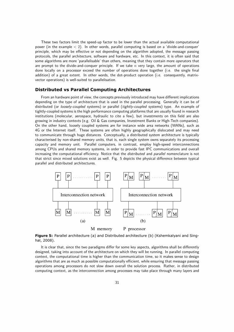
These two factors limit the speed-up factor to be lower than the actual available computationalpower (in the example < 2). In other words, parallel computing is based on a ’divide-and-conquer’principle, which may be effective or not depending on the algorithm adopted, the message passingprotocols, the parallel architecture, software and hardware, etc. In this context, it is often said thatsome algorithms are more ’parallelisable’ than others, meaning that they contain more operators thatare prompt to the divide-and-conquer principle. If we take n very large, the amount of operationsdone locally on a processor exceed the number of operations done together (i.e. the single finaladdition) of a great extent. In other words, the dot-product operation (i.e. consequently, matrix-vector operations) is well-suited to parallelisation.
Distributed vs Parallel Computing Architectures
From an hardware point of view, the concepts previously introduced may have different implicationsdepending on the type of architecture that is used in the parallel processing. Generally it can be ofdistributed (or loosely-coupled systems) or parallel (tightly-coupled systems) type. An example oftightly-coupled systems is the high performance computing platforms that are usually found in researchinstitutions (molecular, aerospace, hydraulic to cite a few), but investments on this field are alsogrowing in industry contexts (e.g. Oil & Gas companies, Investment Banks or High-Tech companies).On the other hand, loosely coupled systems are for instance wide area networks (WANs), such as4G or the Internet itself. These systems are often highly geographically dislocated and may needto communicate through huge distances. Conceptually, a distributed system architecture is typicallycharacterised by non-shared memory units, that is, each single system owns separately its processingcapacity and memory unit. Parallel computers, in contrast, employ high-speed interconnectionsamong CPUs and shared memory systems, in order to provide fast IPC communications and overallincreasing the computational efficiency. Notice that the distributed and parallel nomenclature is notthat strict since mixed solutions exist as well. Fig. 5 depicts the physical difference between typicalparallel and distributed architectures.
Figure 5: Parallel architecture (a) and Distributed architecture (b) (Kshemkalyani and Sing-hal, 2008).
It is clear that, since the two paradigms differ for some key aspects, algorithms shall be differentlydesigned, taking into account of the architecture on which they will be running. In parallel computingcontext, the computational time is higher than the communication time, so it makes sense to designalgorithms that are as much as possible computationally efficient, while ensuring that message passingoperations among processors do not slow down overall the solution process. Rather, in distributedcomputing context, as the interconnection among processes may take place through many layers and
31

it is usually remote, the communication time overcome the computational time. In this regard, it takesonly a little sense to optimise the model from a computational point of view in the case it requiresmany messages to be exchanged among the nodes. The need to carry out distributed computationsusually may regard different reasons: data may be dislocated (e.g. local measurements), there mightbe the need to keep separated memory access from different nodes involved in the computation (e.g.peer-to-peer systems) or simply there might be the possibility to exploit distributed resources moreeffectively.
2.5 Iterative Methods, Distributed Power Flow& Current Prac-tices
As anticipated, this work employs an iterative linear solver for the solution of the sequence ofJacobian linear systems obtained in Section 2.3. Rather than using an iterative method for solvingthe power flow equations faster, we exploit the Krylov-Schwarz approach to carry out a distributedcomputation of power flow equations. A remote computation that only involves a minimal amountof data-sharing have the double advantage to not compromise the overall simulation time whileeffectively keep confidentiality of input data for parties involved in the computation.
Thus far, we introduced concepts on linear solvers in order to provide a comprehensive overviewof the topic. Here, the goal is somewhat to put together all the concepts introduced in the previoussections in the specific context of power flow. We will start from a brief comparison of direct methodsand iterative methods and review in general the potentialities of iterative methods in such a context.
2.5.1 Current Practices and Iterative Methods in Power Flow
From a scientific point of view, power flow problems cannot presently be considered as ’hardlycomplex’ problems to solve. For instance, non-linear systems of equations arising from the discretisa-tion of Partial Differential Equations (PDE) in Computational Fluid Dynamics (CFD) (but in manyother fields as well), are often much bigger in terms of size and present more difficulties to handlethe solution process when compared with power flow problems. In contexts of this kind, where thesize of the problem may even reach n = 109, direct solvers are impractical as the computational costof them (O(n3)) can’t be handled by supercomputing platforms. In power flow context this has notbeen historically the case, mainly for two reasons. First, TSOs solve currently power flow problemswith 103 unknowns, which can be still efficiently handled by direct methods. The other reason beingthat the robustness and the predictable behaviour of direct solvers make them better candidates forcommercial software packages. However, there are at least two important reasons at present thatmay see iterative solvers to overcome the use of direct methods in the future at least for some specificpurposes. As the integration of DERs increases in power grids, the need of grid operators to performmore frequent, more detailed and closer to real-time power system analysis increases at the same pace.Today, the close-to-real-time power flow simulations are carried out through the Fast Decoupled LoadFlow (FDLF) approach, that allows to simplify the power flow problem by losing a little of precisionon the final solution. Despite its speed performances, a drawback of the FDLF approach is the lack ofrobustness, some failure event when the Jacobian is ill-conditioned. Iterative methods offer the possi-bility to speed-up the solution of problems that are particularly computational demanding and proneto parallelisation (e.g. N − k contingency analysis). Furthermore, as present grids are being increas-ingly interconnected at both national and distribution level, the problem size grows; market operationsare more integrated with grid operations, more computational expensive models could be required(e.g. nodal pricing implemented as an optimal power flow problem in AC); sector coupling (or eventhe transmission-distribution coupling itself) may require to carry out coordinated and heterogeneousmodelling among different grids (e.g. gas and electricity networks). These factors may contributeessentially to increase the computational complexity of the power flow problem, while also requiring
32

solvers with different features, able to handle the heterogeneous modelling, able to efficiently run inparallel, etc. This changing paradigm motivates further research in iterative methods for the powersystem context. Relevant insights on performance comparison between iterative methods and directmethods for solving power flow equations are provided in (Idema, 2012), where direct methods andmixed direct-iterative approaches are tested and compared in terms of computational time. (Idema,2012) shows how direct methods for power flow equations stall when the number of buses go over4 ∗ 105, while proving the robustness of Newton-Krylov methods for different sets of generation/loadprofiles. 20 Among the multitude of applications that iterative solvers may have in power system todecrease computational time, a rather different approach is used here. The next sections detail themain idea.
2.5.2 Distributed Approaches
In the past, energy utilities were organized as vertical integrated companies. No competitiveauctions were in place and there was no asymmetry of information among different stages of thesupply chain, since the complete process was managed by a single company. For this reason, themain concern of power flow solver developers in these years was to provide grid operators withfast and above all reliable softwares, mainly based on direct solvers as discussed in the previoussections. Over the last years, the economic and operational framework of the electricity sectorhas undergone a complete restructuring. Transmission and distribution networks at European levelare managed by different entities, which often share boundaries and inter-connect through lines.However, power system analysis tools have not changed: power grids planning and scheduling isstill done by solving power flow and optimal power flow simulations at the transmission level only.In this new configuration of the power system, where the network management is being more andmore distributed and unbundled, we foresee the need of new generation power flow solvers. In theemerging scenario, distributed solvers shall respect at least three main requirements: They need tobe fast, reliable and information/data protective. In literature some distributed solvers for powerflow equations have been already developed over the years, mainly with reference to the DC OPFproblem (e.g. (Mohammadi et al., 2014), (Kargarian et al., 2016)) which represents a considerablesimplification of the AC version. It is worth mentioning that nomenclature can sometimes be a littlemisleading when referring to distributed solvers. For instance, (Kargarian et al., 2016) distinguishesbetween distributed and delocalised approaches. In distributed approaches there is the need of acoordinating entity (i.e. master) that sets the list of operations to execute for coordinated entities(in a master/slave fashion). This does not imply the definition of a global problem at the mastermachine; information may be in fact still inputed from different locations. On the contrary, delocalisedapproaches provide an autonomous framework for entities, where each one can collaborate at samelevel. From a computer science perspective, this last case coincides with the peer-to-peer framework.
Both approaches (distributed/delocalised) share a similar working methodology composed by twomain parts. First, it is needed to re-formulate the global problem into an equivalent21 set of sub-problems. Then, a tailored distributed/delocalised algorithm must be chosen to solve the set ofsub-problems in an organized way. The issue of information protection has not been deserved muchattention in the literature so far. This is mainly due to the fact that traditional application scenariosdo not face the requirements that are arising in the power sector between different utilities. In thiswork we propose a methodology that is highly scalable and only involves a small amount of dataexchange between the parties involved in the power flow computation. The next sections explain ourapproach in detail.
20Note that the simulations carried out in the mentioned work were performed on a single-core platform (i.e. not inparallel).
21The re-formulation must change only in its form. Equivalent means the mathematical problem is not changed andhence must deliver the same solution.
33
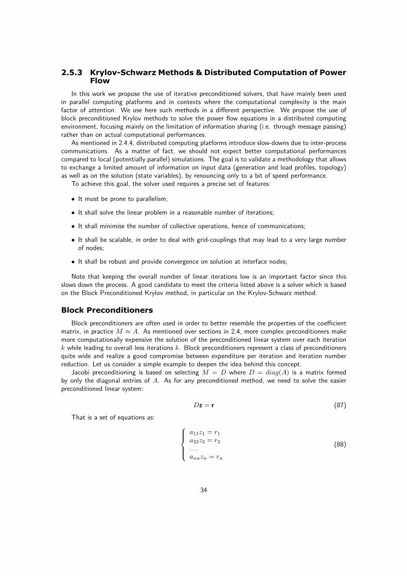
2.5.3 Krylov-Schwarz Methods & Distributed Computation of PowerFlow
In this work we propose the use of iterative preconditioned solvers, that have mainly been usedin parallel computing platforms and in contexts where the computational complexity is the mainfactor of attention. We use here such methods in a different perspective. We propose the use ofblock preconditioned Krylov methods to solve the power flow equations in a distributed computingenvironment, focusing mainly on the limitation of information sharing (i.e. through message passing)rather than on actual computational performances.
As mentioned in 2.4.4, distributed computing platforms introduce slow-downs due to inter-processcommunications. As a matter of fact, we should not expect better computational performancescompared to local (potentially parallel) simulations. The goal is to validate a methodology that allowsto exchange a limited amount of information on input data (generation and load profiles, topology)as well as on the solution (state variables), by renouncing only to a bit of speed performance.
To achieve this goal, the solver used requires a precise set of features:
• It must be prone to parallelism;
• It shall solve the linear problem in a reasonable number of iterations;
• It shall minimise the number of collective operations, hence of communications;
• It shall be scalable, in order to deal with grid-couplings that may lead to a very large numberof nodes;
• It shall be robust and provide convergence on solution at interface nodes;
Note that keeping the overall number of linear iterations low is an important factor since thisslows down the process. A good candidate to meet the criteria listed above is a solver which is basedon the Block Preconditioned Krylov method, in particular on the Krylov-Schwarz method.
Block Preconditioners
Block preconditioners are often used in order to better resemble the properties of the coefficientmatrix, in practice M ≈ A. As mentioned over sections in 2.4, more complex preconditioners makemore computationally expensive the solution of the preconditioned linear system over each iterationk while leading to overall less iterations k. Block preconditioners represent a class of preconditionersquite wide and realize a good compromise between expenditure per iteration and iteration numberreduction. Let us consider a simple example to deepen the idea behind this concept.
Jacobi preconditioning is based on selecting M = D where D = diag(A) is a matrix formedby only the diagonal entries of A. As for any preconditioned method, we need to solve the easierpreconditioned linear system:
Dz = r (87)
That is a set of equations as: a11z1 = r1a22z2 = r2. . .annzn = rn
(88)
34

In the regular Jacobi scheme thus, at each step k each unknown xi is updated regardless of theother. This intuitively works very good on parallel machines. We can divide the set of equations(we call this set S) in equal (or almost equal) SP subsets (S =
⋃SP ), assign them to P nodes
of a parallel machine and solve the problem. Eventually, we can gather the results to build thesolution vector x. As the computation of each xi is completely decoupled from the others, the Jacobiapproach requires many iterations to converge. The Jacobi scheme has been one of the first iterativemethods proposed in literature for solution of linear systems and it is thus not really suitable forreal applications. An improvement of the Jacobi scheme is based on introducing more dependenciesamong the xi variables at each step k, in order to have more accurate solutions. The Gauss-Seidelapproach uses this principle by setting M = L + D, where L is the strict lower triangular matrix ofA. This means we solve, at each step k, a set of equations in the preconditioned residuals zi as22:
a11z1 = r1a11z1 + a22z2 = r2. . .a11z1 + a22z2 + · · ·+ annzn = rn
(89)
These equations can be solved in one step by forward substitution. It is possible to show thatGauss-Seidel converges faster than Jacobi by analysis on the spectral radius of its iteration matrixB. Although Gauss-Seidel improves the convergence properties of the succession x(k), it complicatesits parallel implementation. Let us suppose we use the same approach as before. We call again theset of equations to solve S and divide it into SP subsets (S =
⋃SP ). After that we assign them to
P nodes. The generic node p ∈ 1, . . . , P will need to wait until all the 1, . . . , P − 1 other nodeshave completed the solution of the assigned subset Sp of equations, since the equations in Sp are alldependent on unknowns contained in S1,S2, . . . ,SP−1.
Since the parallelism is a fundamental requirement in order not to share information and keepreasonable time of computation, Gauss-Seidel or similar approaches are not really suited for the work atissue. At the same time we need more effective methods than classical Jacobi scheme, able to deal withbig linear systems without stalling in a huge number of iterations. In this sense, block preconditionerscome in handy. For instance, let consider the extension of the Jacobi preconditioner to its block-form. Instead of taking only the diagonal entries of A, the block-Jacobi method takes diagonal blocksextracted out of A. In other way around we construct a preconditionerM = diag(A11, A22, . . . , APP )made up of subsequent diagonal blocks (we call them App) from A of potential difference size. Wecan either have as many blocks as the processors, or give out multiple blocks to single nodes ofthe parallel system. Here we consider for sake of simplicity that each block is ideally assigned to aprocessor p. The set of preconditioned equations to solve are this time:
A11z1 = r1A22z2 = r2. . .APP zP = rP
(90)
With P the number of total blocks and number of total processors available. Each equation aboveis actually a small linear system to solve, which is as much small as the selected number of totalblocks into which we divide A. Notice that as the dimension of blocks P gets to n, block-Jacobi turnsback to the regular Jacobi scheme, as the dimension of the block would be exactly of one diagonalentry. On the other hand, as P → 1, we are preconditioning the linear system with A itself, hencethe iterative procedure is actually a direct method ending up in exactly one step.
22Here, we are simply assuming A is dense.
35

As for the regular Jacobi scheme, block Jacobi preconditioning works really good in parallel. Inboth cases we can solve the set of linear systems associated with the generic node P independently(i.e. locally). As the number of equations in a generic block q ∈ 1, . . . , Q is usually much lowerthan that of A, we can nicely use factorisation techniques (e.g. LU) to solve the blocks, accordingto the simple computational complexity analysis presented in Section 2.4.4.
A formal mathematical description of block preconditioners can be derived in many ways. Oneway is to do it in terms of projectors23. Here we limit to introduce two operators WT
p (restrictionoperator) and Vu (prolongation operator), which applied together allow to define:
Apu = WTp AVu (91)
Where Apu is a rectangular matrix of dimension p× u, representing the block pu extracted fromA. Dimensionally speaking WT is a q × n matrix and V is a n× u matrix. Note that WT
p , Vu onlyget the components from A without applying any transformation, hence those are matrices made upof only zeros and ones (projectors). In the case of considering the blocks squared, W = V and theequation Eq.(91) becomes:
App = V Tp AVp (92)
Each block is then allocated along the main diagonal of M , overlapping the portion of blockscorresponding to variables in common. This brings to a situation as the one depicted in Fig. 6.
Figure 6: Overlapping Block-Jacobi Preconditioner.
At this stage we have a block diagonal preconditioner M made up of P blocks. A prototypealgorithm for block Jacobi could be the one described in Algorithm 2 below.
Notice that the preconditioning matrix (of dimension n× n) in this case would be:
M =P∑p=1
WTp AppVp =
P∑p=1
WTp (VpAWT
p )Vp (93)
23See Chapter 5 of (Saad, 2003) for the whole procedure.
36
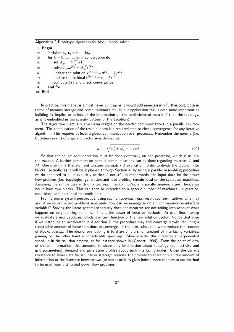
Algorithm 2 Prototype algorithm for block Jacobi solver.1: Begin2: initialize x0, r0 = b−Ax03: for k = 0, 1, . . . , until convergence do4: set Aqq = WT
q AVq5: solve Aqqz(k) = WT
q r(k)
6: update the solution x(k+1) = x(k) + Vqz(k)
7: update the residual r(k+1) = r−Az(k)
8: compute ‖r‖ and check convergence9: end for10: End
In practice, this matrix is almost never built up as it would add unnecessarily further cost, both interms of memory storage and computational time. In our application this is even more important asbuilding M implies to collect all the information on the coefficients of matrix A (i.e. the topology,as it is embedded in the sparsity pattern of the Jacobian).
The Algorithm 2 actually give us an insight on the needed communications in a parallel environ-ment. The computation of the residual norm is a required step to check convergence for any iterativealgorithm. This requires at least a global communication over processes. Remember the norm-2 (i.e.Euclidean norm) of a generic vector w is defined as:
‖w‖ =√w2
1 + w22 + . . . w2
n (94)
So that the square root operation must be done eventually on one processor, which is usuallythe master. A further comment on parallel communications can be done regarding matrices A andM . One may think that we need to store the matrix A explicitly in order to divide the problem intoblocks. Actually, as it will be explained through Section 4, by using a parallel assembling procedurewe do not need to build explicitly neither A nor M . In other words, the input data for the powerflow problem (i.e. topologies, generation and load profiles) remain local on the separated machines.Assuming the simple case with only two machines (or nodes, in a parallel nomenclature), hence wewould have two blocks. This can then be extended to a generic number of machines. In practice,each block acts as a local preconditioner.
From a power system perspective, using such an approach may result counter-intuitive. One mayask: if we solve the two problems separately, how can we manage to obtain convergence on interfacevariables? Solving the linear systems separately does not mean we are not taking into account whathappens on neighbouring domains. This is the power of iterative methods. At each linear sweepwe evaluate a new Jacobian, which is in turn function of the new solution vector. Notice that evenif we introduce an accelerator in Algorithm 2, the procedure may still converge slowly, requiring aremarkable amount of linear iterations to converge. In the next subsection we introduce the conceptof blocks overlap. The idea of overlapping is to share only a small amount of interfacing variables,gaining on the other hand a considerable speed-up. More strictly, this produces an exponentialspeed-up in the solution process, as for instance shown in (Gander, 1996). From the point of viewof shared information, this amounts to share only information about topology (connectivity andgrid parameters), demand and generation profiles about such interfacing nodes. Given the currentresistence to share data for security or strategic reasons, the promise to share only a little amount ofinformation at the interface between two (or more) utilities gives indeed more chances to our methodto be used from distributed power flow problems.
37

Overlapping Block Preconditioners
Another improvement to block preconditioning techniques can be done by allowing the blocksto overlap. By including overlap (thus more dependences) we can improve the convergence of thealgorithm. In other words, the idea of overlap consists in ’sharing’ some variables (and the relatedconstraining equations i.e. the power balances at the related nodes) among processes involved in thecomputation, solve these equations and eventually weight the solution on the shared variables. Theprocedure is then restarted until convergence. The Fig. 7 shows the same (generic) coefficient matrixA, in the two cases: preconditioned by block Jacobi and overlapping block Jacobi. The preconditionerM is constructed in the two cases by extracting only elements inside the red blocks.
(a) Block Jacobi. (b) Overlapping block Jacobi.Figure 7: Block Jacobi preconditioner and overlapping block Jacobi. Only entries inside thered boxes take up into the preconditioning matrix M .
Note that M 6= A, which means when we solve the preconditioned system we do not get theexact solution and hence it motivates the need to iterate the procedure. In the overlapping casewe include more dependencies among variables, making M resembling more A. In this case theoverlapping preconditioner involves common solution on the preconditioned residuals z3, z4 (hencex3, x4). Let us clarify this aspect. Let us write explicitly the equations of the above linear systemand the preconditioned equations with reference to Fig. 7:
a)
a11x1 + a12x1 + a13x3 + a14x4 = b1
a22x2 = b2
a31x1 + a32x2 + a33x3 + a34x4 = b3
a11z1 + a12z2 + a13z3 = r1
a22z2 = r2
a31z1 + a22z2 + a33z3 = r3
= Mupperblock
a42a2 + a43x3 + a44x4 + a45x5 = b4
a52x2 + a53x3 + a54x4 + a55x5 = b5
a44z4 + a45z5 = r4
a52z2 + a53z3 + a54z4 + a55z5 = r5
= Mbottomblock
(95)
38

b)
a11x1 + a12x1 + a13x3 + a14x4 = b1
a22x2 = b2
a31x1 + a32x2 + a33x3 + a34x4 = b3
a11z1 + a12z2 + a13z3 + a14z4 = r1
a22z2 = r2
a31z1 + a32z2 + a33z3 + a34z4 = r3
a42z2 + a43z3 + a44z4 = r4
= Mupperblock
a42a2 + a43x3 + a44x4 + a45x5 = b4
a52x2 + a53x3 + a54x4 + a55x5 = b5
a33z3 + a34z4 = r3
a43z3 + a44z4 + a45z5 = r4
a53z3 + z54z4 + a55z5 = r5
= Mbottomblock
(96)In case a) the equations of upper and bottom block do not share any unknowns. They can be solved
regardless of each other. In a parallel environment, usually one machine (i.e. the master machine)assign sub-problems to other processors (i.e. the slaves). For instance, in our case we can think of amaster solving the upper block and distribute the bottom block to a second processor. Hence, eachprocessor solves locally the owned blocks, in the a) case without exchanging any information (at leastduring the solution process of blocks). On the other hand, to complete the linear sweep we needto update the residual and solution vectors. If we want to avoid inter-communication processes weshall have such coefficients stored locally from the beginning. Using a parallel input can avoid theexchange of this information as well.
In case b) overlap is introduced. We introduce one more equation per block to solve. This means,the upper block now solves with respect z4 as well, whereas the bottom block also gets the value ofz3. As the system of equations differ from upper block to bottom block, we expect different valueson z3, z4 out of each block. How do we update the values of z3, z4 at the end of the linear iteration?A common choice is to weight the results got out of each block, that means according to:
z3 = ξ3z3,ub + (1− ξ3)z3,bb (97)z4 = ξ4z4,ub + (1− ξ4)z4,bb
Where ξ is the weight parameter and the subscripts ub,bb stand for upper block and bottomblock respectively. Let us now analyze what changes in terms of parallel communications. Let usassume a parallel input of data is in place, so that row 1, 2, 3 and 4, 5 of the coefficient matrix arerespectively local on two different processors, which we call proc1 and proc2 respectively. In orderto solve the two blocks on each processor, we need to collect the coefficients a43, a44 from proc2to proc1, and a33, a34 from proc1 to proc2. Once the blocks are solved, the average on interfacingvariables is carried out according to Eq.(97). This can be done either on proc1 or proc2. z3, z4 arethen distributed back to the other processor so that the local solution and residual vectors can beupdated. A last step that involve parallel communication is that of residual norm check, similarly towhat seen in Example 124.
The brief parallel communication analysis provided here shows how is possible to solve a linearsystem by means of block-preconditioners and by only exchanging a limited amount of information(i.e. 1- Coefficients relative to overlapping variables; 2- Solution on interfacing variables; 3- Localsummation of residuals). In the next section we introduce domain decomposition methods. This willallow to introduce a preconditioner (i.e. the Additive Schwarz Method (ASM)), an important pieceof our distributed approach for power flow equations.
24Remember that 〈·, ·〉 = ‖·‖22
39

Domain Decomposition Methods
In science and engineering it is common to formulate modelling equations with reference toa physical domain of interest. These domains are often continuum and involve complex differentialequations that cannot be analytically solved. For this reason, the common practice consists in defininga mesh, that is a discrete domain where differential equations are in some sense averaged from pointto point. Many techniques exist in literature one of them being the finite difference approach. Thisprocess allows to turn the origin differential problem into a set of algebraic equations that can besolved more easily. Although discretisation techniques allow to greatly simplify the problem, typicalalgebraic systems may include up to billions of unknowns, remaining a considerable challenging taskto be solved. Domain Decomposition Methods are used to further simplify the problem. The use ofDDM demonstrated very effectively in handling these kind of huge problems. The principle is thatof divide-and-conquer, which implies a domain division into pieces, with each sub-domain (set ofequations) solved separately. This technique is iterated until convergence at the sub-domain interfacevariables is obtained. In practice, DDMs are used to build preconditioners that can effectively decoupleproblems and help in the solution of complex problems.
It is worth to point out that domain decomposition process can follow different criteria. Wedistinguish these criteria in terms of type of partitioning, that is according to one of the followingcase:
• Vertex Partitioning - vertices are collected into sub-sets that in turn set the decompositioninto sub-domains;
• Branch Partitioning - branches are collected into sub-sets that in turn set the decompositioninto sub-domains;
• Elements Partitioning - elements are collected into sub-sets that in turn set the decompositioninto sub-domains;
For sake of clarity this is depicted in Fig. 8 as well.In the power grids context the above approach is to some extent inverted. We already have
a discrete domain: the graph representing the topology of the grid, on which modelling equations(i.e. power flow equations) are defined are valid bus by bus. In this context we can still use domaindecomposition techniques to further sub-divide the power grid graph into sub-problems. Notice thatusually DDMs are used to decrease the computational complexity of the problems. Again, here wepropose to use them specifically to implement a distributed approach. In the previous sections wepresented some preconditioning approaches that exploit a block partitioning of the coefficient matrixA to break the starting linear system down into linear problems that are easier to solve and parallelise.We then extended the approach introducing the possibility of inputing the data in parallel, hence toavoid the complete share of input information. This has been presented without making any referenceto the graph domain. We will see a specific DDM approach, the ASM procedure, that allow to obtaina preconditioner that is practically equivalent to the overlapping block Jacobi procedure seen throughSection 2.5.3. The only difference of ASM compared to Overlapping Block Jacobi is that we providea mathematical background to decompose the problem starting from the graph-domain and buildingup the preconditioning matrix as a result.
Additive Schwarz Preconditioning
The first Schwarz method proposed an alternating technique to solve Boundary Value Problems(BVPs). A BVP problem is a mathematical problem where the unknown quantities are expressedin terms of their derivatives through a differential equation, with reference to a domain of interest.
40

Figure 8: Type of partitionings. a) Vertex-based, b) Branch-based c) Element-based. (Saad,2003)
Differently from algebraic problems, where it is sufficient to have same number of (independent)equations and unknowns, to find a unique solution of a BVP some boundary conditions are needed aswell. Schwarz demonstrated how is possible to solve a BVP on a generic domain, by sub-dividing itinto sub-BVP and iterating over solutions obtained on such sub-domains. This technique is nowadaysoften used as a preconditioner to decrease complexity of harsh computational problems. A nice wrapup of Schwarz techniques can be found in (J. GANDER, 2008). Here we limit ourselves to a simpleexample. Let us consider Fig. 9:
(a) Domain decomposition of a struc-tured grid.
(b) Matrix representation and Schwarzpreconditioning.
Figure 9: Example of a domain decomposition and its respective matrix representation((Saad, 2003)).
41

In Fig. 9a an example of vertex-partitioning of a structured25 domain into three sub-domains isreported. In Fig. 9b the matrix (we call it A) representing the graph is depicted, where non-zero entriesare represented by the black dots and the dashed lines corresponding to sub-domain decompositiongive a 3 × 3 block structure. We can use this decomposition as a preconditioner by simply settingM = blockdiag(A), where blockdiag is a proper operator extracting the red surrounded blocks. Wehave already seen this operator in the context of Block Jacobi iteration, when we introduced theprolongation and restriction operator and as a result we defined the preconditioner in Eq.(93). InDDM we define these operators with reference to the domain decomposition and according to thepartition criteria chosen (Fig. 8). Let us present it more formally.
Let consider a DDM that divides the starting domain Ω into S subdomains Ωi with i = 1, . . . , S,where the Ωi are not necessarily disjoint (i.e. they can overlap). Then, we define proper Index Sets (IS)that gather indexes of either vertices, branches or elements (depending upon the partitioning criteria)to define which objects belong to a sub-domain Ωi and which not. Using proper nomenclature, theIS Si with reference to sub-domain Ωi can be defined as:
Si = j1, j2, . . . , jni (98)
Where the jk (with k = 1, . . . , ni) are the indexes of elements belonging to subdomain Ωi. ISscan be used to define the prolongation Ri and restriction RTi operators. Let RTi an operator from Ωto Ωi defined as follows: if the generic vector v ∈ Ω, then the vector RTi v ∈ Ωi. Similarly we defineRi: if the generic vector v ∈ Ωi, then the vector Riv ∈ Ω. We can use these operators to define thematrix representing the sub-graph Ai relative to Ωi as follows:
Ai = RiARTi (99)
And define the residual vector ri, the unknown vector xi and right-hand side bi relative to Ωi as:
ri = RTi r (100)xi = RTi xbi = RTi b
The problem at the generic sub-domain Ωi becomes:
Aixi = bi (101)
By solving these sub-problems we can get the solution vector components of x:
x =s∑i=1
Rixi =s∑i=1
RiA−1i bi =
s∑i=1
RiA−1i RTb =
s∑i=1
Ri(RiARTi )−1RTb (102)
As the sub-problems are decoupled (or a little coupled through overlapping variables) the Eq.(102)does not deliver the exact solution. We can thus define a fixed-point linear iteration as:
x(k+1) = x(k) +S∑i=1
RTi A−1i Ri(b−Ax) (103)
25A structured domain (or grid) is a graph where the position of each element follows some regularity principle.In other words we can find the position of a node (and its connectivities) by means of a mathematical expression.In contrast, an unstructured grid is a graph where the position of a generic node must be given through a preciseconnectivity relationship (e.g. a graph incidence matrix). Electrical grids, which are represented through graphs, aretypically unstructured grids.
42

Which compared Eq.(103) with Eq.(70) gives the expression for the ASM preconditioner:
M−1ASM =
S∑i=1
RTi A−1i Ri (104)
As for the Block-Jacobi case, one do not need to explicitly build up the preconditioner matrix.It is possible to set up a procedure to input the sub-domains on each node of a parallel machineand define locally the sub-problems. The ASM procedure allows to keep domains decoupled andto build up local problems based on the domain owned. In case of overlapping variables, messagepassing are needed to add up spaces to b and as many rows as is the number of overlapping variables.Another message passing operation will be needed to check the global norm of the residual vector.The ASM procedure is simple and provides a basis for minimum exchange of communications amongnodes (sub-domains). In practice, accelerators are needed to enlarge the area of convergence and toobtain reasonable time of computation. In the next section we provide an example of the distributedmethodology applied to a simple case.
2.5.4 Distributed Power Flow
In this section we provide an in-dept explanation, with a concrete example, of the different steps ofthe methodology to be followed in order to build a distributed power flow. Wet consider an exampleof partitioning applied to a simple grid case: case13 (see Fig. 10).
Figure 10: Topology of case13, obtained by merging case9.m and case5.m from Matpowerlibraries (Zimmerman and Murillo-Sanchez, 2016).
In the classic application of a DDM the domain is divided into sub-domains that are possiblyassigned to different processors of a parallel machine. For instance, one can apply the branch-partitioning depicted in Fig. 10 with reference to the case13, and divide it into case5 and case9.The case5 and case9 are then assigned to different processors according to the partitioning criteriachosen. As the aim is to protect grid operators from information sharing about their input data, weshall adopt a different strategy here. We consider again only two machines. The parallel solution ofpower flow problem follows an approach that can be conceptually divided in two stages:
43
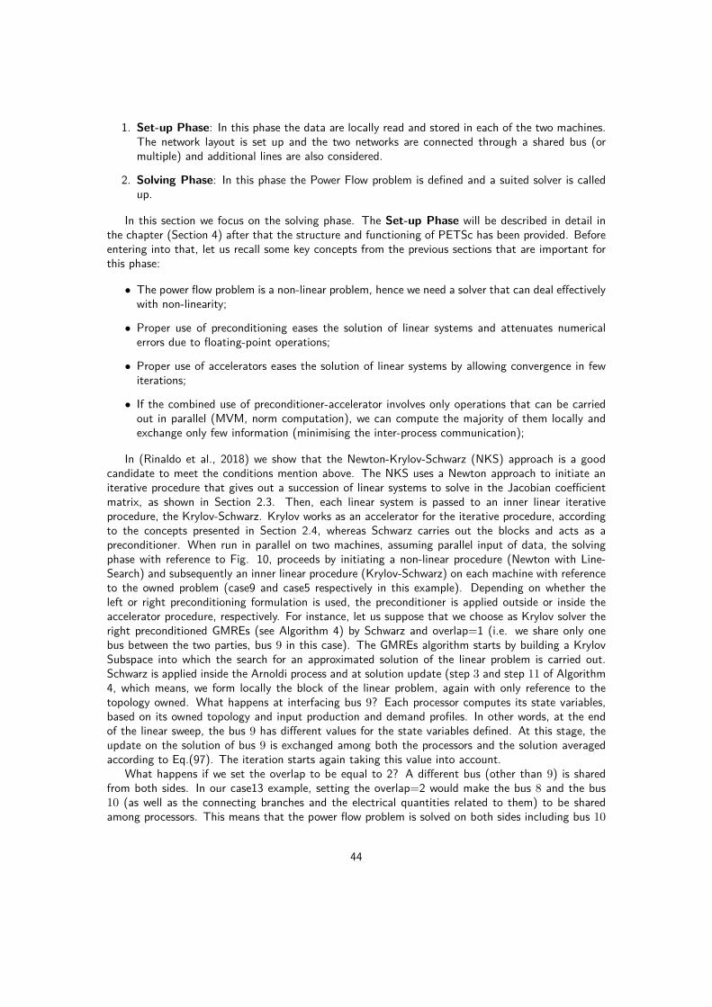
1. Set-up Phase: In this phase the data are locally read and stored in each of the two machines.The network layout is set up and the two networks are connected through a shared bus (ormultiple) and additional lines are also considered.
2. Solving Phase: In this phase the Power Flow problem is defined and a suited solver is calledup.
In this section we focus on the solving phase. The Set-up Phase will be described in detail inthe chapter (Section 4) after that the structure and functioning of PETSc has been provided. Beforeentering into that, let us recall some key concepts from the previous sections that are important forthis phase:
• The power flow problem is a non-linear problem, hence we need a solver that can deal effectivelywith non-linearity;
• Proper use of preconditioning eases the solution of linear systems and attenuates numericalerrors due to floating-point operations;
• Proper use of accelerators eases the solution of linear systems by allowing convergence in fewiterations;
• If the combined use of preconditioner-accelerator involves only operations that can be carriedout in parallel (MVM, norm computation), we can compute the majority of them locally andexchange only few information (minimising the inter-process communication);
In (Rinaldo et al., 2018) we show that the Newton-Krylov-Schwarz (NKS) approach is a goodcandidate to meet the conditions mention above. The NKS uses a Newton approach to initiate aniterative procedure that gives out a succession of linear systems to solve in the Jacobian coefficientmatrix, as shown in Section 2.3. Then, each linear system is passed to an inner linear iterativeprocedure, the Krylov-Schwarz. Krylov works as an accelerator for the iterative procedure, accordingto the concepts presented in Section 2.4, whereas Schwarz carries out the blocks and acts as apreconditioner. When run in parallel on two machines, assuming parallel input of data, the solvingphase with reference to Fig. 10, proceeds by initiating a non-linear procedure (Newton with Line-Search) and subsequently an inner linear procedure (Krylov-Schwarz) on each machine with referenceto the owned problem (case9 and case5 respectively in this example). Depending on whether theleft or right preconditioning formulation is used, the preconditioner is applied outside or inside theaccelerator procedure, respectively. For instance, let us suppose that we choose as Krylov solver theright preconditioned GMREs (see Algorithm 4) by Schwarz and overlap=1 (i.e. we share only onebus between the two parties, bus 9 in this case). The GMREs algorithm starts by building a KrylovSubspace into which the search for an approximated solution of the linear problem is carried out.Schwarz is applied inside the Arnoldi process and at solution update (step 3 and step 11 of Algorithm4, which means, we form locally the block of the linear problem, again with only reference to thetopology owned. What happens at interfacing bus 9? Each processor computes its state variables,based on its owned topology and input production and demand profiles. In other words, at the endof the linear sweep, the bus 9 has different values for the state variables defined. At this stage, theupdate on the solution of bus 9 is exchanged among both the processors and the solution averagedaccording to Eq.(97). The iteration starts again taking this value into account.
What happens if we set the overlap to be equal to 2? A different bus (other than 9) is sharedfrom both sides. In our case13 example, setting the overlap=2 would make the bus 8 and the bus10 (as well as the connecting branches and the electrical quantities related to them) to be sharedamong processors. This means that the power flow problem is solved on both sides including bus 10
44

and 8 and by following the same procedure explained for the case with only one bus overlap. Noticethat the DDM aspect of Schwarz is a bit hidden in the latter description. In practice, this takespartially place through the Set-Up Phase, where the graphs of sub-networks are built locally on eachprocessor, rather than on a master machine and then distributed to the slave machines. Based onthis step, the solver understands that the local network is actually part of a bigger network sharedwith another entity and builds the solution procedure accordingly. In this sense, the Jacobi blocks arebuilt up starting from the local graph, but knowing that each block is mathematically part of a biggerproblem, exactly as it would be done after a proper local ’decomposition’ on a master machine andsend through to a slave machine. Another mention goes on parallel communication analysis. Thishas been done in this work strictly with reference to stationary block-preconditioned methods 2.5.3.In practice adding up accelerators (i.e. Krylov solvers) causes the procedure to be more complexand structured in more steps (see Annex 2 for GMREs full algorithm). A precise analysis of parallelcommunications of the Krylov-Schwarz solver shall be employed to understand exactly the informationpassed through machines. On the other hand, a Krylov accelerator involves mainly MVM and normcomputations which can be easily carried out in parallel. This means the computation can be carriedout by performing only few collective operations. Further analysis on parallel communications ofKrylov-Schwarz solvers are let to future works.
45

3 PETSc
Almost anything that relates to natural phenomena is described through complex time-varying,and sometimes non linear, PDEs. Their solution is obtained in scientific computing through accuratediscretisation techniques, that approximate the PDE models locally, turning the problem into a setof algebraic equations. Even though systems of algebraic equations are much easier to solve whencompared with differential ones, the design of effective numerical techniques is not a simple task.Such issues can be of the following type:
1. Problems should be addressed with the best tailored techniques, in order to decrease the com-putational complexity and to obtain good levels of method’s robustness;
2. parallelisation is almost always needed due to the computational complexity of the problems,which often makes the implementation of certain numerical techniques non-trivial.
Tackling both these issues is still a big challenge for many scientific problems. Numerical scientistsstruggle nowadays for developing scientific computing tools that address those problems. Among themany libraries developed in the world there is the Portable, Extensible Toolkit for Scientific Compu-tation (PETSc). PETSc is "a suite of data structures and routines for parallel solution of complexscientific problems" according to the definition that its developers at Argonne National laboratorygive. This set of libraries has been developed purposely for parallel computing applications. PETScis meant to be used both as a solver and as an API to program with. This allowed many librariesto be developed starting from PETSc, such as: Hypre, SuperLU, Trilinos and many others. PETSchas been used for simulations in a broad range of subjects: fluid dynamics, material science, rocketscience and many others. It can be used for application codes in both C, C++, Fortran and Python.The libraries enable easy customisation and extension of both algorithms and implementations. Thisapproach promotes code reuse and flexibility, and separates the issues of parallelism from the choiceof algorithms. Moreover, PETSc successfully handles the complexities introduced by MPI (messagepassing interface) by managing completely on itself the message passing operations.
3.1 PETSc Structure
PETSc consists of a variety of libraries and each library manipulates a certain family of objects.The organisation is hierarchical as shown in Figure 11. The most simple objects (Matrices, Vectorsand Index Sets) are built on top of BLAS (Basic Linear Algebra Subprograms) and MPI. BLAS is aportable library of routines for performing matrix-vector operations while MPI is the interface thatmanages inter process communications. For more information about MPI see (Pacheco, 1998).On top of Matrices, Vectors and Index Sets, user can find KSP (Kryolv solvers) and PC (Precondi-tioners) family objects. KSP consists of over thirty Krylov subspace methods, for iterative solution oflinear systems. PC objects are used in conjunction with KSP to perform preconditioned linear itera-tions. KSP is integrated with underlying direct solvers (LU factorisation, QR factorisation) that areused to solve subproblems generated by either the KSP iteration scheme or by domain decompositionprovided by PC.The most complex objects built in PETSc are represented by SNES (Scalable Nonlinear EquationsSolvers) and TS (time-steppers) solvers, that are built on top of KSP and PC. SNES is a collectionof nonlinear solvers and TS is used for solving time-dependent PDEs.All the solvers available can be simply selected by the user at runtime. A more detailed explanationof PETSc routines can be found in the Users Manual (Balay et al., 2018a). In the next sectionsfurther information on PETSc application codes and solvers will be given and on how the programcopes with large networks.
46

Figure 11: PETSc hierarchy. The red encircled solvers are those relevant for the Power Flowproblem and dealt in this work.
3.2 PETSc representation of networks: DMNetwork and DM-Plex
This section shows how PETSc manages structured and unstructured grids. Networks are usedcommonly to represent power distribution systems, water and gas distribution, communication, trans-portation or electric circuits. DM (Domain Management) are libraries used for managing interactionsbetween mesh data structures and mathematical objects like vectors and matrices. DMNetwork is aclass of functions in PETSc that is used for network representation. It allows the user to manage thetopology and the physics of large scale networks and the coupling with linear, non linear or time vari-ant solvers. In (Maldonado et al., ) different application frameworks are presented. DMNetwork datastructure in PETSc provides efficient and convenient ways for network decomposition. It is possibleto split the domain in n sub-domains (through a domain decomposition) or divide a multi-physicssystem into different single physical subsystems (field-split).In order to build a network object, all the components have to be recorded. In power system, thenetwork components are mainly of four types: buses, branches, generators and loads (protectiondevices are not taken into account at this stage). Once those information are recorded DMNetworkbuilds a mathematical model that could be a set of linear, non linear or time-dependent equations.The system of equations is then solved using KSP, SNES or TS libraries.Some features of this framework include:
47

• the possibility of assigning different degrees of freedom to nodes (buses) or edges (branches);
• the possibility of assigning network components (e.g. loads or generators) to each bus;
• the support on network partitioning among different processors;
• the creation of the Jacobian operator (associated to the network) as well as the vectors forresidual evaluation;
• the storing of information on ghost nodes that need to perform communication with the otherprocessors;
• the full compatibility with KSP, SNES and TS solvers.
DMNetwork is actually built on top of DMPlex, a data management object that embeds thetopology of unstructured grids to provide a range of functionalities common to many scientific ap-plications (Lange et al., 2015b). The topological connectivities between the components in DMPlexare expressed as a Directed Acyclic Graph (DAG). A DAG is a graph where vertices are connectedthrough edges, each edge is directed from a vertex to another so that there is no way to start froma vertex and loop back to it again.
(a) Edge and vertex numbering (b) Connectivity in a DAGFigure 12: Example of a tetrahedron and its respective DAG representation (Lange et al.,2015a).
Fig. 12 illustrates a Directed Acyclic Graph representation of a simple tetrahedron. Component’senumeration starts from the entire figure (0), vertices are enumerated from 1 to 4, faces from 5 to8 and edges from 9 to 14. The DAG is divided in layers and each component belongs to a certainlayer. Once the DAG is built there are several operations inside DMPlex that allow the user toextract elements of a grid, see connectivities, mapping data layout and distribute data among parallelprocessors.Moreover DMPlex provides other functionalities for grid partitioning and domain decomposition.There are graph partitioning methods already implemented in PETSc while many others can befound in external libraries such as Chaco (Hendrickson and Leland, 1993) or ParMetis (Karypis et al.,1997). Six different partitioners can be chosen. They allow the user to decompose the problem inthe most suitable way for a certain application code; by default PETSc decomposes the grid in sucha way that all the processors own more or less the same number of elements.Once that creation and distribution steps are carried out, a network object contains:
• a partitioned graph representation of the problem
48

• a memory space allocation for the problem’s unknowns in each vertex and edge
• a set of physical data in each bus
• an implicit nonzero structure determination of the Jacobian matrix
3.3 Solving Power Flow Equations using PETSc
In Section 2 the power flow problem has been presented and the most suitable numerical techniquesused over the course of time have been briefly discussed. It has been shown how the power flowproblem needs a proper numerical method to handle the non-linearity and an inner linear solver. InPETSc, it is done by setting an outer SNES solver and an inner KSP solver, possibly preconditionedthrough a PC object. An example written in C (power.c) to solve power flow problems in PETSc canbe found in the following folder:
$PETSC_DIR/src/snes/examples/tutrtials/network/power/
The C code can be divided in three main stages:
1. Reading stage
2. Set up stage
3. Solving stage
Reading Phase
The input file is a Matpower test case. In this example the reference grid is case9.m which canbe found in the Matpower libraries.MATPOWER is a package of free, open-source Matlab-language M-files for solving steady-state powersystem simulation and optimisation problems such as power flow (AC and DC) or Optimal PowerFlow (OPF).Matpower includes also a set of test cases, ranging from small to large size power grids, up to closeapproximations of the European High Voltage Transmission Grid. Details about entries of Matpowercaseformat can be accessed from MATLAB by typing help caseformat. Cases are made of 6 fields, 4of which are structs. Those structs include data for buses, generators, branches and generator costs.For more details on MATPOWER test cases the reader can consult (Zimmerman and Murillo-Sanchez,2016). In the following the categories of each matrix in data struct are shown for sake of clarity. Busstruct is a n× 13 matrix (where n is the number of buses) containing the following columns:
bus_i type Pd Qd Gs Bs area Vm Va baseKV zone Vmax Vmin
Generator data matrix is a ngen × 21 matrix, where ngen is the number of generators, divided asfollow:
bus Pg Qg Qmax Qmin Vg mBase status Pmax Pmin Pc1 Pc2 Qc1min Qc1max Qc2minQc2max ramp_agc ramp_10 ramp_30 ramp_q apf
Branch data matrix is a m× 13 matrix where m is the number of branches
fbus tbus r x b rateA rateB rateC ratio angle status angmin angmax
Finally generator costs data matrix has the following structure:
49

1 startup shutdown n x1 y1 ... xn yn2 startup shutdown n c(n-1) ... c0
Additionally MATPOWER libraries include since 2015 a list of cases which correspond to real world cases.In (Josz et al., ) different test cases are presented: RTE test cases represent the French very-highvoltage grid, while PEGASE test cases give a snapshot of the European high-voltage grid. Those datacan be read by PETSc application code power.c, previously mentioned. Note that they should beprovided as an input at runtime.From an implementation point of view the first part of the code is the following:/* READ THE DATA */if (!crank) /* READ DATA *//* Only rank 0 reads the data */ierr = PetscOptionsGetString(NULL,NULL,"-pfdata",pfdata_file,PETSC_MAX_PATH_LEN
-1,NULL);CHKERRQ(ierr);ierr = PetscNew(&pfdata);CHKERRQ(ierr);ierr = PFReadMatPowerData(pfdata,pfdata_file);CHKERRQ(ierr);User.Sbase = pfdata->sbase;numEdges = pfdata->nbranch;numVertices = pfdata->nbus;ierr = PetscMalloc1(2*numEdges,&edges);CHKERRQ(ierr);ierr = GetListofEdges_Power(pfdata,edges);CHKERRQ(ierr);
The conditional operator if(!crank) implies that only rank 0 processor is in charge of readingdata. Using PetscOptionsGetString() it is possible to provide a string for a particular optionin the database. In this case the string "-pfdata" allows to select the test case that is going to beused at runtime. An empty PETSc object is then created using PetscNew() function. The funtionPFReadMatPowerData() takes as an input the datafile provided from Matpower library and fills allthe fields in pfdata struct, which are:typedef structPetscScalar sbase; /* System base MVA */PetscInt nbus,ngen,nbranch,nload; /* # of buses,gens,branches, and loads */VERTEX_Power bus;LOAD load;GEN gen;EDGE_Power branch; PFDATA
The fields VERTEX_Power, LOAD, GEN and EDGE_Power are structs as well and they are declaredin power.h header file. When all the fields are correctly filled the function GetListofEdges_Power()creates an array edges of size 2m where m is the number of branches. It is created in this way:for (i=0;i<m;i++)edges[2*i]= from_bus; /* the first column values in mpc.branch struct */edges[2*i+1]= to_bus; /* the second column values in mpc.branch struct */
After this procedure the reading phase can be considered complete.
50
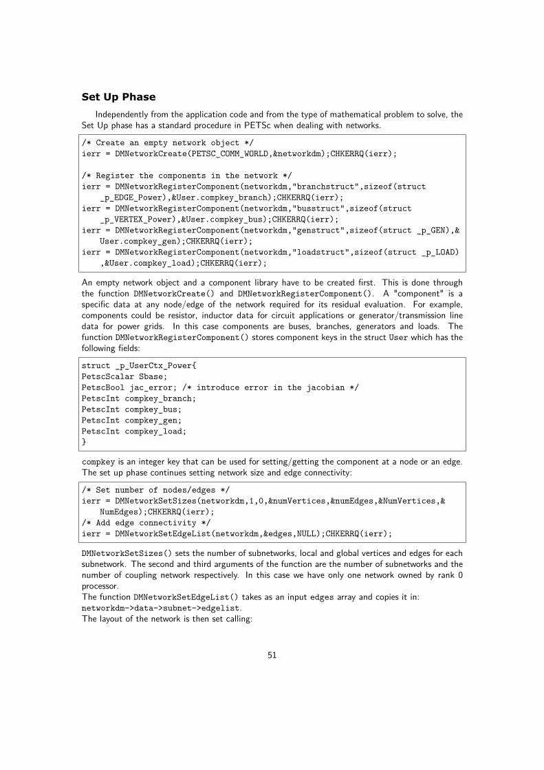
Set Up Phase
Independently from the application code and from the type of mathematical problem to solve, theSet Up phase has a standard procedure in PETSc when dealing with networks.
/* Create an empty network object */ierr = DMNetworkCreate(PETSC_COMM_WORLD,&networkdm);CHKERRQ(ierr);
/* Register the components in the network */ierr = DMNetworkRegisterComponent(networkdm,"branchstruct",sizeof(struct
_p_EDGE_Power),&User.compkey_branch);CHKERRQ(ierr);ierr = DMNetworkRegisterComponent(networkdm,"busstruct",sizeof(struct
_p_VERTEX_Power),&User.compkey_bus);CHKERRQ(ierr);ierr = DMNetworkRegisterComponent(networkdm,"genstruct",sizeof(struct _p_GEN),&
User.compkey_gen);CHKERRQ(ierr);ierr = DMNetworkRegisterComponent(networkdm,"loadstruct",sizeof(struct _p_LOAD)
,&User.compkey_load);CHKERRQ(ierr);
An empty network object and a component library have to be created first. This is done throughthe function DMNetworkCreate() and DMNetworkRegisterComponent(). A "component" is aspecific data at any node/edge of the network required for its residual evaluation. For example,components could be resistor, inductor data for circuit applications or generator/transmission linedata for power grids. In this case components are buses, branches, generators and loads. Thefunction DMNetworkRegisterComponent() stores component keys in the struct User which has thefollowing fields:
struct _p_UserCtx_PowerPetscScalar Sbase;PetscBool jac_error; /* introduce error in the jacobian */PetscInt compkey_branch;PetscInt compkey_bus;PetscInt compkey_gen;PetscInt compkey_load;
compkey is an integer key that can be used for setting/getting the component at a node or an edge.The set up phase continues setting network size and edge connectivity:
/* Set number of nodes/edges */ierr = DMNetworkSetSizes(networkdm,1,0,&numVertices,&numEdges,&NumVertices,&
NumEdges);CHKERRQ(ierr);/* Add edge connectivity */ierr = DMNetworkSetEdgeList(networkdm,&edges,NULL);CHKERRQ(ierr);
DMNetworkSetSizes() sets the number of subnetworks, local and global vertices and edges for eachsubnetwork. The second and third arguments of the function are the number of subnetworks and thenumber of coupling network respectively. In this case we have only one network owned by rank 0processor.The function DMNetworkSetEdgeList() takes as an input edges array and copies it in:networkdm->data->subnet->edgelist.The layout of the network is then set calling:
51

/* Set up the network layout */ierr = DMNetworkLayoutSetUp(networkdm);CHKERRQ(ierr);
Once that a bare layout is defined components and number of variables can be set in each node/branch.The process in charge of adding components and variables is rank 0 process again.
if (!crank) genj=0; loadj=0;ierr = DMNetworkGetEdgeRange(networkdm,&eStart,&eEnd);CHKERRQ(ierr);for (i = eStart; i < eEnd; i++) ierr = DMNetworkAddComponent(networkdm,i,User.compkey_branch,&pfdata0->branch[i
-eStart]);CHKERRQ(ierr);ierr = DMNetworkGetVertexRange(networkdm,&vStart,&vEnd);CHKERRQ(ierr);for (i = vStart; i < vEnd; i++) ierr = DMNetworkAddComponent(networkdm,i,User.compkey_bus,&pfdata->bus[i-vStart
]);CHKERRQ(ierr);if (pfdata->bus[i-vStart].ngen) for (j = 0; j < pfdata->bus[i-vStart].ngen; j++) ierr = DMNetworkAddComponent(networkdm,i,User.compkey_gen,&pfdata->gen[genj++])
;CHKERRQ(ierr);if (pfdata->bus[i-vStart].nload) for (j=0; j < pfdata0->bus[i-vStart].nload; j++) ierr = DMNetworkAddComponent(networkdm,i,User.compkey_load,&pfdata->load[loadj
++]);CHKERRQ(ierr);/* Add number of variables */ierr = DMNetworkAddNumVariables(networkdm,i,2);CHKERRQ(ierr);
After that all the components have been successfully added, the network is ready to be distributedamong different processors.
ierr = DMSetUp(networkdm);CHKERRQ(ierr);
This function has to be called every time as it provides a signal that the network is ready to bedistributed. The distribution is made by:
ierr = DMNetworkDistribute(&networkdm,0);CHKERRQ(ierr);
By default PETSc distributes the network object in such a way that each processor owns more orless the same number of elements. The distribution process can be modified changing the partitionerused by DMNetworkDistribute().
Solving Phase
Once that each processor has received its sub-problem, the solving phase starts. The masterprocessor communicates the solving procedure to use and a local solver is built up on each processor.
52

The PETSc library provides three layers of solvers: KSP, SNES, and TS to solve these problems,respectively.
Table 2: PETSc Solvers
Solver Name Description Mathematical Form
KSP and PC Krylov Subspace Methods and Preconditioners Ax − b = 0SNES Non Linear Solver F (x) = 0TS Time Stepping Solver F (t, x, x) = 0
As already mentioned, in power flow context according to steady state approximation a non-linearsystem of equation of the type F (x) = 0 has to be solved. Using Newton’s method the problem canbe approximated to a set of linear equation:
J(xk)∆xk = −F (xk)xk+1 = xk + ∆x
(105)
The function F (xk) and the Jacobian matrix J(xk) have to be evaluated at each iteration andEq.(105) has to be solved iteratively to obtain the approximated solution xk.PETSc takes care of parallel distribution, preallocation, partitioning and setting up data structures.The user needs to provide two functions, one for F (x) evaluation and one for the Jacobian J(x).The application flow starts creating a non linear solver context and adapting DMNetwork object toit. After that both residual function and Jacobian have to be created. The non linear problem is thenready to be solved.
/* HOOK UP SOLVER */ierr = SNESCreate(PETSC_COMM_WORLD,&snes);CHKERRQ(ierr);ierr = SNESSetDM(snes,networkdm);CHKERRQ(ierr);ierr = SNESSetFunction(snes,F,FormFunction,&User);CHKERRQ(ierr);ierr = SNESSetJacobian(snes,J,J,FormJacobian_Power,&User);CHKERRQ(ierr);ierr = SNESSetFromOptions(snes);CHKERRQ(ierr);ierr = SNESSolve(snes,NULL,X);CHKERRQ(ierr);
With the function SNESSetFromOptions() it is possible to set parameters for non linear solverat runtime. For example it is possible to set the maximum number of iterations, absolute andrelative tolerances, type of solver (Newton, Richardson, GMREs) and many others. Once thatSNESSetFromOptions() is invoked all the underlying layers’ options are enabled.To summarize, rank 0 processor takes as an input a Matpower test case and saves it into a struct. Itbuilds a network object and distributes it among the processors involved in the computation. Powerflow equations are then solved using Newton Raphson method coupled with a direct preconditionedsolver. Both linear and non linear methods can be chosen between all the ones implemented in PETSclibraries.
53
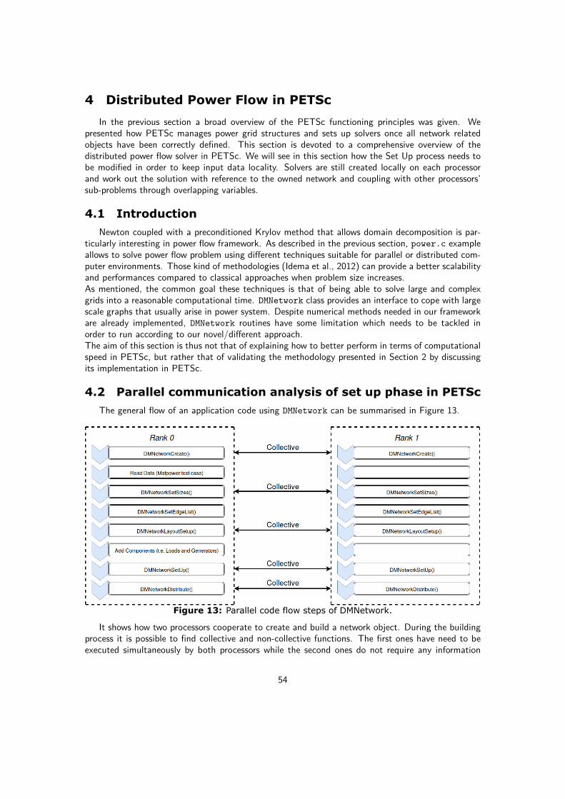
4 Distributed Power Flow in PETSc
In the previous section a broad overview of the PETSc functioning principles was given. Wepresented how PETSc manages power grid structures and sets up solvers once all network relatedobjects have been correctly defined. This section is devoted to a comprehensive overview of thedistributed power flow solver in PETSc. We will see in this section how the Set Up process needs tobe modified in order to keep input data locality. Solvers are still created locally on each processorand work out the solution with reference to the owned network and coupling with other processors’sub-problems through overlapping variables.
4.1 Introduction
Newton coupled with a preconditioned Krylov method that allows domain decomposition is par-ticularly interesting in power flow framework. As described in the previous section, power.c exampleallows to solve power flow problem using different techniques suitable for parallel or distributed com-puter environments. Those kind of methodologies (Idema et al., 2012) can provide a better scalabilityand performances compared to classical approaches when problem size increases.As mentioned, the common goal these techniques is that of being able to solve large and complexgrids into a reasonable computational time. DMNetwork class provides an interface to cope with largescale graphs that usually arise in power system. Despite numerical methods needed in our frameworkare already implemented, DMNetwork routines have some limitation which needs to be tackled inorder to run according to our novel/different approach.The aim of this section is thus not that of explaining how to better perform in terms of computationalspeed in PETSc, but rather that of validating the methodology presented in Section 2 by discussingits implementation in PETSc.
4.2 Parallel communication analysis of set up phase in PETSc
The general flow of an application code using DMNetwork can be summarised in Figure 13.
Figure 13: Parallel code flow steps of DMNetwork.
It shows how two processors cooperate to create and build a network object. During the buildingprocess it is possible to find collective and non-collective functions. The first ones have need to beexecuted simultaneously by both processors while the second ones do not require any information
54

exchange and can be executed separately. "Read Data" and "Add Components" steps are carried outby rank 0 process which is usually considered as the master node (in a master-client paradigm). Inthis case only the latter has access to the network input data and until the DMNetworkDistribute()function is not called all grid information is kept by the rank 0 node. Successively (after the call)graph elements and associated data are distributed among the nodes. Fig. 14 shows how PETScmanages and distributes a simple seven buses network.
(a) Simple 7 buses network. PETSc enumeration
(b) Directed Acyclic Graph (DAG) for the network above
(c) Splitted network on two processors. Shared elements are moved tohigher rank processor
Figure 14: Network management in PETSc
Network components enumeration starts from edges and it continues with buses. All componentsare registered in a Direct Acyclic Graph (DAG). Branches are stored in the first layer (first row inFigure 14b) while buses in the layer below. Network decomposition is done through edges. Accordingto Figure 14b, branches 0, 1, 2 are assigned to rank 0 and 3, 4, 5 to rank 1, buses are allocatedaccordingly to edge partition. By default shared elements (bus 9 in this case) are moved to the higherrank processor.The two nodes involved can be considered as two different entities at national or international level.Within this framework the asymmetry of information is evident as one entity owns all the dataregarding topology, generation and demand profiles.
55

4.3 Parallel Assembling procedure
In order to obtain a distributed input of data as well as a parallel assembling of the network somemodifications are indeed necessary. Fig. 15 illustrates the idea behind a parallel assembling procedure.Input data are located remotely on two different workstations. Each processor takes as an input acase data file (its own data network). In reality, bus 6 on rank 0 and bus 3 on rank 1 in Figure 15arefer to the same bus (bus 9 in Figure 14a).
(a) Simple 7 buses network where input data are on two different nodes
(b) Directed Acyclic Graph (DAG) for the previous network: in thedefault set up procedure DAGs are not connected
(c) Directed Acyclic Graph (DAG) for the previous network using aparallel assembling procedure
(d)Figure 15: Network management in PETSc using a parallel assembling procedure
56

If the Read Data function is not a collective operation, the two networks are considered twoseparate grids instead of being two portions of the same network. In other words DAG in Figure 15bdoes not have any connectivity between ranks. This has to be modified in order to obtain a graphlike the one in Figure 15c.To make this, edge layer identifiers need to be contiguous. In this sense the number of branches onrank 0 has to be added to every branch identifier on rank 1. Thus Reading phase needs collectivityin order to exchange information regarding the total number of branches. Rank 0 sends to rank 1an integer corresponding to the total number of branches on master node, rank 1 changes branchenumeration accordingly.Bus layer identifiers change their enumeration during the layout set up step. Among other tasks, thefunction DMNetworkLayoutSetUp() overwrites bus indexes in order to obtain a consecutive enumer-ation right after for branches. The modified flow of the application code using parallel assemblingprocedure is shown in Fig. 16.
Figure 16: Modified flow
The main differences that can be highlighted are the following:
1. Both nodes execute all the functions
2. The Read data phase is collective
3. The Layout set up of the network allows a parallel assembling procedure
In a wider context this application flow can be seen as two entities running a coordinated powerflow. Each entity has its own remote control centre where information regarding topology, demandand generation profiles are stored. The two grids are connected through a certain number of inter-connection branches thus the solution of one sub-network is dependent on the characteristics of theneighbouring grid.
4.4 Solving Phase
After that the previous procedure has been completed, the network elements and correspondingDAG are correctly set up among the processes involved in the computations. It is not necessary toinvoke DMNetworkDistribute() since the network is already correctly split between the processors.Power flow equations are then solved iteratively, voltage magnitudes and phase angles are found ateach node of the network. It is important to stress that the solution obtained in this way is the samethat it will be obtained by one entity running a global power flow on the two sub-networks together.
57

In order to prove the well-functioning of this concept a test case was set. Two small test cases inMATPOWER libraries have been selected: case9.m and case5.m respectively. They have been mergedtogether considering that the first bus in case5.m corresponds to the ninth bus in case9.m. Theresulting network is illustrated in Figure 17. Bus 1 is the slack node, buses 2, 3, 11, 12, 13 are PVbuses while the others are PQ buses. Input data were distributed among two different processors inthe configuration shown in Figure 18.
Figure 17: case13.m
Figure 18: case13.m divided in two workstations
case9.m was assigned to master node and case5.m to client node. Reading and set up proceduresfollow the steps previously described. Once the network object has been correctly set up, power flowequations are solved by SNES library in PETSc. The Jacobian linear system is solved using GMREspreconditioned with overlapping Additive Schwarz.
58

The results in terms of voltage magnitude and phase angles are reported for both processors in Table3. Bus ownership reflects input data locality. Once the voltage profiles are found as a solution ofthe power flow problem, active and reactive power flow in each branch can be calculated. Table 4illustrates the amount of power flows in each branches subdomain. Those data can be easily savedremotely on each workstation depending on the network ownerships.
Table 3: Results: Voltage Magnitude and Phase Angle per node
BusNumber
rank 0 rank 1
Voltage Magnitude Phase Angle Voltage Magnitude Phase Angle1 1 02 1 -0.071033 1 -0.10864 0.9957 -0.1635 0.9839 -0.21536 1.0063 -0.15827 0.9922 -0.20788 1.0047 -0.17269 0.9943 -0.3571 0.9943 -0.357110 0.9878 -0.412611 1 -0.402112 1 -0.400113 1 -0.3492
Table 4: Results: Active and Reactive Power in each branch
RankBranch From bus injection To bus injection
From To P [MW] Q [MVar] P [MW] Q [MVar]0 1 4 280.613 30.314 -280.613 15.5720 4 5 56.325 -4.020 -55.779 -8.5040 5 6 -34.221 -21.496 34.700 -11.8760 3 6 85.000 -8.736 -85.000 13.0150 6 7 50.299 -1.139 -49.992 -17.1230 7 8 -50.008 -17.876 50.233 4.9320 8 2 -163.000 15.885 163.000 0.7210 8 9 112.767 -20.817 -108.726 10.5730 9 4 -219.214 37.259 224.288 -11.5511 9 10 194.837 8.598 -193.755 1.5151 9 12 137.839 -29.732 -137.228 35.1861 9 13 -129.736 -76.696 129.881 75.0461 10 11 -106.244 -101.515 106.481 102.0551 11 12 -6.481 0.3175 6.483 -0.9791 12 13 -169.254 20.953 170.119 -12.984
Note that this approach allows convergence with a tolerance of less than 10−8 on the absolutenorm26. Overlapping variables converge at the same solution on both sides (machines) with the same
26The convergence check is done also on relative norm of the residual vector
59

convergence check above. Another important aspect that can be highlighted is that the solution isfound keeping a reasonable convergence time (4.39 10−2 seconds on two 8-node 32 GB RAM machine,each node being an Intel Xeon E3-1275 3.50 Ghz running on an Ubuntu 17.10 64-bit GNU/Linuxdistribution and mounting a network card of 1 Gbit/s).From an implementation point of view, it is wort mentioning that PETSc allows to evaluate simulationperformances with profiling options. In fact PETSc routines automatically log performance dataand they can be printed using different profiling options. The option -log_view prints an overallperformance summary, including times, floating-point operations, computational rates and messagepassing activity.The bottleneck is usually the type of interconnection chosen between the workstations. In (Rinaldoet al., 2018) some simulation tests by means of Newton-Krylov-Schwarz on a distributed systemarchitecture are presented. Two interconnected European high transmission voltage grids were testedusing different type of network configurations. The results showed the feasibility of performing thedistributed calculation remotely, keeping the overall simulation times quite low (only few times slowerthan locally considering two grids in the order of thousands nodes sizes).
60

61

5 Applications
This section discusses the potential application framework of distributed/delocalised approachesto power flow equations. In particular, we focus on two cross-border frameworks: 1) the TSO-TSOcongestion management in Europe; 2) the TSO-DSO coordination at the transmission-distributioninterface. With respect to the first case we focus mainly on the Capacity Calculation Methodology(CCM) currently in place in Europe to tackle congestion management issues. As we will see, this isactually a complex procedure made up of many steps, during which TSOs and various stakeholderscollaborate in order to provide the market with the bounds for Capacity Allocation (CA) process.
For the second case the discussion will be more qualitative. As DSOs are currently facing are-organisation in terms of roles to accommodate RES penetration at distribution level and currentlydo not generally carry out power flow computations yet, the methodology is presented in a ’softer’way. However, it is worth mentioning that numerous TSO-DSO coordination schemes that requirethe DSO to run power flow computations are being presented in research and pilot projects (e.gSmartNet, Coordinet), underpinning the importance of the topic at issue.
5.1 Congestion Management at European Level
In order to harmonise and liberalise the EU’s internal energy market, measures have been adoptedsince 1996 to address market access, transparency and regulation, consumer protection, supportinginterconnection, and adequate levels of supply. These measures aim to build a more competitive,customer-centred, flexible and non-discriminatory EU electricity market with market-based supplyprices. In so doing, they strengthen and expand the rights of individual customers and energy com-munities, address energy poverty, clarify the roles and responsibilities of market participants andregulators and address the security of the supply of electricity, gas and oil, as well as the develop-ment of trans-European networks for transporting electricity and gas(Gouarderes, 2019). A numberof big improvements has been already achieved in these years: looking at market integration, forinstance, we have today a single price coupling algorithm, called EUPHEMIA (EU + Pan-EuropeanHybrid Electricity Market Integration Algorithm) which calculates electricity prices across Europe (for27 countries). Operated by eight NEMOs (Nominated Electricity Market Operators), the algorithmallocates simultaneously electricity and capacity between bidding zones27, a process known as implicitallocation or market coupling. The aim of market coupling is that of maximising economic surplusby using efficiently all the available resources. Inter-connectors are hence fundamental to achieve thisgoal being the means to connect different European bidding zones.
In theory two exclusive situations should be observed when looking at the flows at the intercon-nection points between bidding zones: one, in which the inter-connectors are partially used (belowtheir maximum capacity) and the price is the same in the two neighbouring bidding zones; the other,in which the line is congested so that there is a price differential between the two bidding zones, thatis a market splitting. In reality, what one can see is that very often there are situations in which theinter-connector is only partially used but there is a price differential between the connected biddingzones. Even more paradoxical than that, there were cases in the past mainly due to explicit allocationof capacity between bidding zones in which electricity was flowing from zones of higher prices to thoseof lower prices.
In (ACER and CEER, 2018), the Agency for the Cooperation of Energy Regulators (ACER) andthe Council of European Energy Regulators (CEER) argue that low level of cross-zonal transmissioncapacity currently observed in their monitoring might be due to congestions not properly addressedby the current bidding zone configuration in Europe. That is, structural congestions might be present
27Bidding zones in Europe mainly coincide with national borders, apart from some cases as Sweden and Italy whichhave four and six bidding market zones, respectively.
62
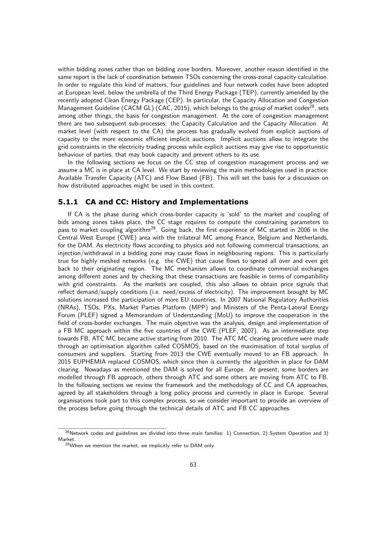
within bidding zones rather than on bidding zone borders. Moreover, another reason identified in thesame report is the lack of coordination between TSOs concerning the cross-zonal capacity calculation.In order to regulate this kind of matters, four guidelines and four network codes have been adoptedat European level, below the umbrella of the Third Energy Package (TEP), currently amended by therecently adopted Clean Energy Package (CEP). In particular, the Capacity Allocation and CongestionManagement Guideline (CACM GL) (CAC, 2015), which belongs to the group of market codes28, setsamong other things, the basis for congestion management. At the core of congestion managementthere are two subsequent sub-processes: the Capacity Calculation and the Capacity Allocation. Atmarket level (with respect to the CA) the process has gradually evolved from explicit auctions ofcapacity to the more economic efficient implicit auctions. Implicit auctions allow to integrate thegrid constraints in the electricity trading process while explicit auctions may give rise to opportunisticbehaviour of parties, that may book capacity and prevent others to its use.
In the following sections we focus on the CC step of congestion management process and weassume a MC is in place at CA level. We start by reviewing the main methodologies used in practice:Available Transfer Capacity (ATC) and Flow Based (FB). This will set the basis for a discussion onhow distributed approaches might be used in this context.
5.1.1 CA and CC: History and Implementations
If CA is the phase during which cross-border capacity is ’sold’ to the market and coupling ofbids among zones takes place, the CC stage requires to compute the constraining parameters topass to market coupling algorithm29. Going back, the first experience of MC started in 2006 in theCentral West Europe (CWE) area with the trilateral MC among France, Belgium and Netherlands,for the DAM. As electricity flows according to physics and not following commercial transactions, aninjection/withdrawal in a bidding zone may cause flows in neighbouring regions. This is particularlytrue for highly meshed networks (e.g. the CWE) that cause flows to spread all over and even getback to their originating region. The MC mechanism allows to coordinate commercial exchangesamong different zones and by checking that these transactions are feasible in terms of compatibilitywith grid constraints. As the markets are coupled, this also allows to obtain price signals thatreflect demand/supply conditions (i.e. need/excess of electricity). The improvement brought by MCsolutions increased the participation of more EU countries. In 2007 National Regulatory Authorities(NRAs), TSOs, PXs, Market Parties Platform (MPP) and Ministers of the Penta-Lateral EnergyForum (PLEF) signed a Memorandum of Understanding (MoU) to improve the cooperation in thefield of cross-border exchanges. The main objective was the analysis, design and implementation ofa FB MC approach within the five countries of the CWE (PLEF, 2007). As an intermediate steptowards FB, ATC MC became active starting from 2010. The ATC MC clearing procedure were madethrough an optimisation algorithm called COSMOS, based on the maximisation of total surplus ofconsumers and suppliers. Starting from 2013 the CWE eventually moved to an FB approach. In2015 EUPHEMIA replaced COSMOS, which since then is currently the algorithm in place for DAMclearing. Nowadays as mentioned the DAM is solved for all Europe. At present, some borders aremodelled through FB approach, others through ATC and some others are moving from ATC to FB.In the following sections we review the framework and the methodology of CC and CA approaches,agreed by all stakeholders through a long policy process and currently in place in Europe. Severalorganisations took part to this complex process, so we consider important to provide an overview ofthe process before going through the technical details of ATC and FB CC approaches.
28Network codes and guidelines are divided into three main families: 1) Connection, 2) System Operation and 3)Market.
29When we mention the market, we implicitly refer to DAM only.
63

5.1.2 Relevant CACM articles
Moving back to the CACM, its content can be divided into the following categories:
• Optimal definition of bidding zones;
• Calculation of capacities between bidding zones;
• Allocation of cross-zonal capacities with MC;
• Management of residual congestions with remedial actions (e.g. re-dispatch, counter-trading).
Each one includes sub-sections providing detailed procedures to follow. Member States can thenimplement them only with little freedom. For major amendments, TSOs must present modificationsproposal of the CACM to NRAs and ACER for final approval.
The CACM details how the CC process must be carried out in Europe. The main steps of theregulation includes:
• Requirements for definition of Capacity Calculation Regions (CCRs);
• Requirements for definition of a Common Grid Model (CGM);
• Generation and Load Data Provision (CGM) methodology;
• Capacity Calculation Methodology (CCM);
• Coordinated Capacity Calculation (CCC) process.
The CCRs are those EU regions where the CC process is meant to be carried out by TSOs. Fig. 19shows the first coordinated proposal made by all TSOs on CCRs on the. Following to the decision ofACER on the 17th November 2016, the CWE CCR and the Central East Europe (CEE) CCR have beenmerged into a unique CCR, namely the CORE CCR. Some follow-ups as public consultations amongTSOs have been launched to discuss small amendments on CCRs. In general, ACER expects thenumber of CCRs to decrease over time. Merging CCRs give the advantage of reducing uncertaintiesof CC process due to inter-dependency (only slightly present) of some CCRs.
In simple wording, the CCRs are nothing but borders among bidding zones30. This implies thateach TSO acting on the borders must take part to the CC process. The CCC process starts by askingeach bordering TSO to prepare an Individual Grid Model (IGM), according to Article 19 of CACM,part of the section dedicated to CGM (Articles 14-19). The IGM is an approximated model of theeach TSO’s transmission system, relevant for the purpose of CCC. IGMs are then merged to form theCGM. Notice that Article 19 provides several requirements to the IGMs. In practice, an IGM mustinclude all the ingredients to allow load flow computations on it (i.e. generation and load profiles,topology; all updated according to the best possible forecasts). Article 16 develops requirementsof the GLDP procedure and requires "TSO to jointly develop a proposal for the delivery of thegeneration and load data required to establish the CGM". Articles 20-26 provides the CCM, in shortwhat parameters (Critical Network Elements (CNE) and Contingencies (CNEC), Generation ShiftKeys (GSKs), Power Transfer Distribution Factors (PTDFs), Reliability Margins (RMs), RemedialActions (RAs)) to compute and how. Articles 27-30 provide more details on the CC based on ATCand FB approaches.
Currently, the process to collect the information from TSOs, to merge the IGMs into the CGM andto carry out the capacity calculations is under the responsibility of the Regional Security Coordinators(RSCs). These are companies owned or controlled by TSOs. RSC are also in charge of proposing
30Note that a bidding zone border may have more than one TSO operating its own control area (e.g. Germany).
64

Figure 19: Capacity Calculation Regions firstly proposed by all TSOs according to Article 15of 1222/2015 (CACM).
improvements to the quality of computation. As the process of cross-border capacity ends up, theresults obtained by RSC are passed back to TSOs. TSOs start a validation phase of the results withreference to their CNEs and contingencies. The capacity validation and allocation constraints areshared with other relevant TSOs of the CCR and with RSC. Eventually, the RSC provides the NEMOswith validated capacities and allocation constraints for the market coupling stage.
Note that the actual CCM and CCC may differ among the CCRs as the CACM provides indicationsand requirements on methodology proposal, but not strict rules on its implementation. In otherwords, the CACM requires TSOs to formulate their own CCM and CCC procedure according to theiroperating needs, scenarios and cost-benefit analysis. An example of proposed CCC by the NordicCCR is reported in Fig. 20.
Of course, each specific CCM and CCC adopted for each CCR must be formally prepared andratified by NRAs and ACER. As mentioned, in European Transmission Network (ETN) both ATCand FB CC approaches are used, depending on the ’meshed’ extent of interconnections. The CACMprovides strong incentives onto using FB approach for meshed interconnections. In the next sectionsATC and FB CC procedures are presented. The discussion about ATC approach is dealt quite generally,
65

Figure 20: CCC process proposal by TSOs member of the Nordic CCR (Nordic-TSOs, 2018).
with no specific CCR reference. The FB CC is discussed with reference to the CC approach used bythe CORE CCR ((CORE-TSOs, 2018)).
5.1.3 Capacity Calculation Mechanisms: ATC
The ATC procedure aims to calculate the Available Transfer Capacity between two neighbouringregions (in either directions) that can be sold in the Day Ahead and Intraday markets without en-dangering the security of each (CCR) system. In order to define the Available Transfer Capacity forsuccessive trading over market stages, RSC and TSOs must coordinate to compute three fundamentalparameters: the Total Transfer Capacity (TTC), the Transmission Reliability Margin (TRM) and theNet Transfer Capacity (NTC). Before this, let us introduce the necessary inputs required for theircomputation.
1. Critical Network Element Contingency (CNEC):Generally, grid elements (branches, tie-lines, transformers, etc.) present physical limits thatmust be respected at any time during their operation. TSOs usually associate to each of theseelements a maximum stationary allowed current (Imax) and optionally a maximum temporarycurrent. The physical limits to respected during operation are of three main types:
• Thermal limits• Voltage limits• Stability limits
A correct estimation of Imax is not a simple task to deal with. For instance, weather conditionsneed to be taken into account, for instance, during summer the cables are cooled less effectively
66

than on other seasons. Starting from the definition of an Imax, it is possible to calculate amaximum allowed power flow Fmax on a component by the following relation:
Fmax =√
3 Imax,cont V cosφ (106)
Where V and cosφ are the reference voltage and the power factor of the tie-line, respectively.In the past, ATC methodologies required TSOs to identify branches that could be sensitiveto cross-border exchanges, in the sense that operated in real-time could result too close totheir power flow limits (Fmax). For each CB TSOs had to assess also the impact of possibleCritical Outages (COs) of other components. The set of all CB and COs formed the so-calledCBCOs set. Following to the introduction of CACM, CBCOs have been replaced by the CNECs- Critical Network Elements Contingencies. In practice, CNECs are very similar to CBCOs withthe only distinction being that they are more broadly defined, thus include a wider range ofcontingencies and of possibly critical components.
2. Generation Shift Keys (GSKs):The GSKs define how changes in the net position of the concerned bidding zone is mapped ongenerators. For instance, let us consider a generator Gi that has associated a GSKi = 10%and let us consider a change in the net position amounting to 100MW . This means that theoutput of Gi will change of a quantity equal to 10MW (with the sign defined by the sign ofthe net change of the zone). GSKs are usually associated to generating units that are marketdriven and that can provide flexibility in changing electric power output.
3. Remedial Actions (RAs):A list of RAs is prepared by each TSO and integrated in the IGM. Each RA details the expectedimpact (i.e. the flow change) over each CNE under a specific contingency. This information ispassed to RSC in order to let it compute the best RA to apply whenever a certain contingencyis faced and to consider ex-ante the impact that this will have on the flow pattern. This is alsocalled Remedial Action Optimisation (RAO) process.
The GSKs, RAs and CNECs list together with the IGM (individual TSO topology + GLDP) arecollated in a file known as the D-2 Congestion Forecast (D2CF) that allow for congestion forecast ofthe individual TSO situation. The D2CF must respect precise requirements in terms of data formatand quality. The Common Information Model (CIM) exchange sets the standard for informationexchange regarding not only D2CF, but more generally for any data exchange involving TSOs, DSOs,NEMOs, etc. The RSC brings together all the IGMs to assemble the CGM (or base case). The basecase consist of a global congestion forecast for the CCR. The RSC starts its calculation process fromthe base case with the aim to assess the maximum bilateral inter-connection capacity among twobidding zones.
1. TTC Calculation:The TTC value is defined as the maximum exchange program between two areas, compatiblewith Operational Security Policy (OSP) applicable at each system (typically N-1 security crite-ria) and with tie-line technical limits. This value represents the Total Capacity of the line andhence must be never surpassed. In other words, capacity calculations must only make a portionof such total capacity available to the market and anticipate possible emergency situations,unscheduled flows, uncertainties on generation and load estimations, etc.
2. TRM Calculation:In real-time cross-border power exchanges might deviate from the forecasted values mainly dueto imperfect information from market players and unexpected events (e.g. weather changes).An example of such deviations is balancing power injected/withdrawn from the grid through
67

frequency control regulation. The evaluation of TRM can be done by the TSOs according topast experiences or using statistical methods. Usually TRM values are typically agreed andfixed for a long time period (e.g. 1 year). In other situations this is just fixed to an activepower value (e.g. Elia reserve 250MW at each border) or as a percentage of TTC.
3. NTC Calculation:Given the TTC and TRM the NTC on a given cross-border interconnection is calculated as:
NTC = TTC − TRM (107)
The NTC value represents the maximum amount of power that can flow through a tie linetaking into account the uncertainties in future network conditions. Two neighbouring TSOsshould calculate NTC for the same border in both directions. As usually TSOs find differentNTC values, they need to reach an agreement on which value to set. As always, the mostconservative approach is chosen for sake of security of the system: the lower value is taken ascommon NTC value.
A possible flow diagram of the calculation process is depicted in Fig. 21. The methodology isstraightforward. Let consider A and B as two adjacent bidding zones. The responsible RSC usesstep-wise changes (e.g. +100MW from A to B) and monitor at each step how changes in theforecast net position impact the power flows over critical grid elements (CNECs). In the case inwhich a security violation on any CNECs is observed, the last net position is recorded as the maximumallowable power flow - i.e. the TTCA→B . The opposite is done as well to compute TTCB→A in theopposite direction. At this stage, the NTCs are simply obtained by subtracting the TRMs:
NTCA→B = TTCA→B − TRMA→B
NTCB→A = TTCB→A − TRMB→A (108)
As such, the NTCs are not the ATCs yet. As we are considering day-ahead time frames, remindthat prior to DAM, Forward Markets take place. This means that part of the NTC might be alreadysold through previous market sessions (in forward markets). The ATCs are hence obtained as:
ATCA→B = NTCA→B − LTAsA→BATCB→A = NTCB→A − LTAsB→A (109)
The couple of values ATCA→B , ATCB→A represent a trading quantity that can be offered to themarket. A graphical representation of this concept is given in Fig. 22.
The ATC quantity is passed to the MC algorithm as an allocation constraint (or input). As ageneral rule, we can say that this value tends to be estimated in a more conservative way as thedelivery is far in time. As the time of delivery approaches, the level of uncertainty decreases and morecapacity can be allocated. This is indeed what happens in the IDM, where usually additionally ATCquantity is offered to the market.
5.1.4 Capacity Calculation Mechanisms: Flow Based
The FB procedure is considered more accurate to calculate the capacity transfer between biddingzones especially for meshed grids. Rather than constraining the capacity of tie lines as for the ATCCC approach, the FB CC approach takes directly into account the arising flows over CNEs resultingfrom cross-border exchanges. The FB CC procedure starts locally for each TSO, similarly as for ATCapproach. Each TSO prepares a set of input data that later will be collected by the RSC for FB
68

Figure 21: Flow-diagram for TTC and NTC calculation.
parameters computation. This includes again an IGM, containing an approximated representation ofTSOs’ grid and input data describing load and generation patterns forecast (GLDP). Other inputs arethe GSKs, some (additional) External Constraints (ExtC), the Flow Reliability Margin (FRM), LTAs(Long-Term Acquisitions) and possible information about HVDC interconnections. Let us detail thecomputation of some input parameters for the FB CC procedure.
• CNECs: The selection process follow the same rules of ATC. The difference here is that eachTSO explicitly associate to each CNE a maximum allowed flow Fmax. Different contingenciesare considered for each CNE according to the TSO security policy, to form the CNECs (CNEwith a Contingency) elements.
69
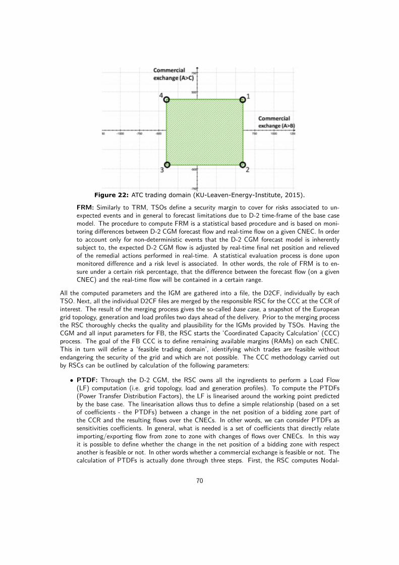
Figure 22: ATC trading domain (KU-Leaven-Energy-Institute, 2015).
FRM: Similarly to TRM, TSOs define a security margin to cover for risks associated to un-expected events and in general to forecast limitations due to D-2 time-frame of the base casemodel. The procedure to compute FRM is a statistical based procedure and is based on moni-toring differences between D-2 CGM forecast flow and real-time flow on a given CNEC. In orderto account only for non-deterministic events that the D-2 CGM forecast model is inherentlysubject to, the expected D-2 CGM flow is adjusted by real-time final net position and relievedof the remedial actions performed in real-time. A statistical evaluation process is done uponmonitored difference and a risk level is associated. In other words, the role of FRM is to en-sure under a certain risk percentage, that the difference between the forecast flow (on a givenCNEC) and the real-time flow will be contained in a certain range.
All the computed parameters and the IGM are gathered into a file, the D2CF, individually by eachTSO. Next, all the individual D2CF files are merged by the responsible RSC for the CCC at the CCR ofinterest. The result of the merging process gives the so-called base case, a snapshot of the Europeangrid topology, generation and load profiles two days ahead of the delivery. Prior to the merging processthe RSC thoroughly checks the quality and plausibility for the IGMs provided by TSOs. Having theCGM and all input parameters for FB, the RSC starts the ’Coordinated Capacity Calculation’ (CCC)process. The goal of the FB CCC is to define remaining available margins (RAMs) on each CNEC.This in turn will define a ’feasible trading domain’, identifying which trades are feasible withoutendangering the security of the grid and which are not possible. The CCC methodology carried outby RSCs can be outlined by calculation of the following parameters:
• PTDF: Through the D-2 CGM, the RSC owns all the ingredients to perform a Load Flow(LF) computation (i.e. grid topology, load and generation profiles). To compute the PTDFs(Power Transfer Distribution Factors), the LF is linearised around the working point predictedby the base case. The linearisation allows thus to define a simple relationship (based on a setof coefficients - the PTDFs) between a change in the net position of a bidding zone part ofthe CCR and the resulting flows over the CNECs. In other words, we can consider PTDFs assensitivities coefficients. In general, what is needed is a set of coefficients that directly relateimporting/exporting flow from zone to zone with changes of flows over CNECs. In this wayit is possible to define whether the change in the net position of a bidding zone with respectanother is feasible or not. In other words whether a commercial exchange is feasible or not. Thecalculation of PTDFs is actually done through three steps. First, the RSC computes Nodal-
70

to-Slack (N2S) PTDFs by varying the injection/withdrawals per each node and by registeringthe change in the flow per each CNEC. Then, by using the GSKs turns the N2S PTDFs intoZone-to-Slack (Z2S) PTDFs coefficients. This is done to scale the change of the node tothe change in the net position of the zone. Eventually, the Z2S PTDFs are used to computeZone-to-Zone (Z2Z) PTDFs coefficients.
• Net Position Flow FNCP : We define the FNCP as the flow of active power through a CNECgiven a certain Net Commercial Position (NCP) relative to bidding zone A. This practicallyrepresent the expected power flow as the market clears, according to the final NCP . Asmentioned, many other factors intervene in the real-time so that this flow is only an estimationgiven the output of the market. With reference to a CNEC i, the FNCP can be computed byusing the previous defined Z2S PTDFs as follows:
FNCP,i = Fref,i +N∑A=1
PTDFA,i(NCPA −NCPA,ref ) (110)
Where NCPA,ref is the net commercial position of bidding zone A at base case NCP .
RAMs: The RAMs define the remaining available margin per each CNEC. Available marginswill result by subtracting out of the maximum possible Fmax, all the factors that ’take up’ aportion of the Fmax. This is done according to:
RAMs = Fmax − FRM − FAV − FNCP (111)
Where the FAV term stands for ’Final Adjustment Value’ and may be or may be not done byeach TSO at the validation stage (i.e. after the RSC send back the CGM and the computedresults to all CCR TSOs).
Once the RAMs of each CNEC are computed, the whole set of constrains can be used to build up atrading domain similar to the ATC one Fig. 22. In a plane of net commercial positions NCPA→B-NCPB→A, the set of equations Eq.(111) form a set of straight lines that provide the limits to thetrading domain. The situation is shown in Fig. 23, where a comparison between the FB and the ATCtrading domain is depicted.
In Fig. 23 the domain representation is limited to the exchanges among three bidding zones A,Band C. In such trilateral case, the set of constrains are simply straight lines. Notice that a CCR thatinvolves a set of generic N bidding zones involve higher dimensional space of representation for thetrading domain. More precisely, the trading domain of a generic bidding zone A with respect all theother B,C, . . . lies in a N dimensional space. Each constrain would be represented as an hyperplaneof dimension N .
From an economical and an engineering point of view, the interesting fact that can be drawn fromFig. 23 is the wider resulting domain obtained through the FB approach with respect to the ATC. Awider trading domain allows to increase the amount of cross-border exchanges, to obtain greater priceconvergence between zones and as a consequence an higher social welfare. Generally, methodologiesthat can enlarge the trading domain without decreasing the level of operational security are of greatrelevance in a context where RES production may be substantially higher in some countries in short-times, and hence offer convenient exchange opportunities.
5.1.5 Limitation of Current Practices
Some well-known limitations exist on ATC and FB CC approaches. In the ATC approach (Fig.23) the trading domain is usually constrained by a set of horizontal and vertical lines that produce
71

Figure 23: FB and ATC trading domains (KU-Leaven-Energy-Institute, 2015).
in general a rectangular domain31. This means that if we reduce the power flow exchange between,for instance, A and B, this do not result in a higher capacity between A and C. The ATC approachthus assesses the capacities bilaterally, and by taking a conservative approach on potential loop flowsand transit flows (Fig. 24) which might result from neighbouring cross-border exchanges32.
In other words, the ATC approach do not use a real mathematical model to describe the flowsresulting from neighbouring zones, but rather takes conservative assessments on them based onexperience. On the other hand, the FB approach incorporates the inter-dependency of zones througha physical model of power flows (although through a linearised approach). In this way, since anycommercial exchange among neighbouring zones is translated into a change in the flow on eachcritical component (CNECs), we can get a much better modelling of the constraints. For example,if we follow a straight line constraint in Fig. 23 we see that a change of commercial exchangeon one border (say A-B) has an impact on another border (A-C). Since FB CC can be considereda more precise approach to model cross-border commercial exchanges, one may ask why in someEuropean CCRs the ATC procedure is still in place. One of the reasons is that bidding zones that arepoorly meshed with their neighbours can be modelled effectively with ATC approach (e.g Italy-GreeceCCR). In these cases ATC and FB approaches give in fact the same results, with the advantagefor ATC of being a simpler procedure which involve less parameters to compute (and indeed lesscoordination). On the contrary, Central Europe is characterised by highly meshed interconnectionsand flows through different bidding zones show a strong interdependency with each other. Hence,considering the ATC approach as ’limited’ with respect to the FB makes sense only for those regionsthat are sufficiently meshed. On this matter, the CACM states (in Article 20, point 7) that:"TSOsmay jointly request the competent regulatory authorities to apply the coordinated net transmissioncapacity approach if the TSOs concerned are able to demonstrate that the application of the capacitycalculation methodology using the flow based approach would not yet be more efficient comparedto the net transmission capacity approach and assuming the same level of operational security inthe concerned region" which shows how the CACM strongly stimulates for implementation of FBCCC where significant benefits can be obtained at same level of operational security. An example
31The domain is squared when the cross-border capacities are symmetric in either direction.32Loop flows are those flows that start off and get back into its originating bidding zone. Transit flows are flows
that before reaching the destination pass through neighbouring bidding zones.
72

Figure 24: Example of bilateral trade (yellow arrows) and resulting physical flows over thegrid (blue arrows). Commercial flows do not translate in physical flows, but rather createseveral loop and transit flows according to Kirchhoff’s Law.
of ongoing implementation of FB in place of ATC is that one concerning the Nordic CCR, whichis expected to end in 2022 (Nordic-TSOs, 2018). After a cost-benefit Nordic TSOs have indeedidentified FB as a solution that can bring benefits to CCC process. As ATC and FB CCC shall bedifferently applied depending on the topology of CCR, possible improvements to both procedures canbe foreseen. In previous sections we discussed the methodologies in a generic framework. We canconceptually divide a CCM in three steps:
1. ATC/FB inputs preparation (IGM) at TSOs control centres;
2. RSC collects input information from TSOs through a dedicated digital platform according tothe Common Information Exchange Model and builds the CGM;
3. RSC sends back to TSOs the results of the ATC/FB computation. The TSOs validate theresults and the trading domain is passed to the market.
Currently these steps are only partially coordinated among TSOs though it is known that by increasingcoordination at various stages may yield a better estimation of ATC and FB parameters and deliver
73

a more precise estimation of the available cross-border capacity. For instance, during the first stepeach TSOs builds its own IGM and makes an estimation of generation and demand within its controlarea. At this stage, the internal distribution of flows is obviously not known. Cross-border flows areonly estimated based on historical data. Inputs are asked to neighbouring TSOs, but the extent ofcoordination is though low. This means that the actual preparation of data concerning RAs, CNECs,GSKs, GLDP and forecast on topology state at day of delivery can be imprecise thus leading toimprecise load flow computations performed at this initial stage.Over the second step the RSC builds up the CGM and carries out the CCC process. A similardiscussion can be carried out for the third step, where the validation process is only left to the TSOdirectly interested without involving neighbouring TSOs which are ‘indirectly’ involved.With respect to the CCC of meshed CCRs, another source of inaccuracy is given by the linearisationof power flow problem for the computation of the PTDFs coefficients. One may think to perform amore accurate estimation of the PTDFs coefficients by carrying out an AC load flow computation.As a result, the trading domain would be more accurately defined, at the cost of not having a linearproblem to solve. This actually involves a complex and broad discussion involving DAM market designand the Price Coupling Algorithm (PCA) which is not the scope of this work.
5.1.6 Advantages of Distributed Capacity Calculation
In the previous sections we highlighted some limitation of the current approaches to compute theavailable capacity trading domain. Proposing more accurate calculations for processing parameters,either in the context of ATC or FB CC, may allow to decrease the level of uncertainty on future flowsdistribution and grid conditions, hence enlarging the trading capacity domain offered to the market.In practical terms, this means to be able to exchange more power as needed, and in turn obtainingthe benefit of a more efficient allocation of generating power. A distributed approach to computepower flow equations at the initial stage of the CCC may allow to plan coordinately the inputs, toforesee the impact of contingencies, to cope with solar and wind uncertainty and possible outages,on each other assets. This could be done with the advantage of not sharing detailed informationabout owned assets, e.g. the graph topology of the transmission system, generation and demandprofiles. The distributed power flow methodology can be intended as a mean to bridge the gaps dueto asymmetry of information among TSOs, without entailing them to share sensitive information. Byintroducing more detailed information gives in turn the benefits of having as a result a more reliablecomputation. The same reasoning can be applied as mentioned for the validation stage, after theRSC CCC process ends up.Another important factor concerns the time-frame. The problem of correctly calculating and allocatingcross-border capacity can be seen as a chicken-and-egg problem. At the real-time the uncertainty onproduction, demand and possible contingencies is null, as production and demand profiles are well-defined. On the other hand, the definition of a schedule for suppliers and consumers is only definedonce capacities are defined and allocated to the market. The distributed power flow methodologypresented here allows for a fully automated approach that only requires the TSOs to produce topology,generation and load inputs for the coordinated calculation. The time required for the simulation isclose to that of local ones provided that a fast interconnection among control centres is available(at least 1Gbit/s). With automation and fast simulation times, the approach may allow TSOs tobring their analysis closer to the real-time, or to evaluate more scenarios at the same time. Anotherremark is that by decomposing the load flow problem into sub-problems, for instance by means of themethodology presented here, the mathematical formulation of the problem does not change. Thismeans that the solution that is obtained is exactly the same that would be obtained in the case a uniqueentity owned all the input data for the load flow and solved it locally. As the possibility to have a uniqueTSO managing the whole ETN does not seem realistic at the moment, a concrete solution to align
74

TSOs positions could be that of relying on distributed/delocalised approaches. A final considerationgoes to the possibility of scaling up the methodology. As the grid becomes more active at lower voltagelevels, TSOs may require to include in their power flow computation information about underlyingdistribution networks. This makes the computation more complex and more computational expensiveand may require TSOs to face new investments in dedicated computational infrastructures. Thecosts of such can be shared among TSOs if they adopt a distributed approach. As the computationalburden is shared among grid operators, the computational power required locally is reduced. In thenext final section we briefly discuss possible applications of distributed approaches to the mentionedcase of TSO-DSO interface.
5.2 TSO-DSO Coordination
This section aims at giving a short overview on how new policy provisions might change therole of TSOs and DSOs and especially their interaction. In the coming years the higher penetrationof wind and solar distributed power production, the stochastic recharging connection behaviour ofEVs, the appearance of new market actors (prosumers, energy communities), the possibility to havestorage system integration, are expected to remarkably have a direct impact on distribution gridsmanagement and indirectly on transmission system operation. The old role of the DSO as passivenetwork operator moved by the ‘fit and forget’ approach, is expected to change into a new active rolemore similar to that of TSOs in transmission networks management. First generation network codesand guidelines (those under the Third Energy package) have already started to address the change,by stimulating TSO and DSO to cooperate and to define coordination schemes on some operationaltasks. Under the CEP new Network Codes (NCs) are expected to be developed from ENTSO-e andthe new EU DSO entity in the next years. In the second part of this section possible applicationsof distributed approaches in view of the emerging changes are briefly discussed. The most naturalframework of application being the transmission-distribution networks interface.
5.2.1 Operational & Policy Context in Distribution Grid Management
The entry into force of TEP in 2009 has brought important changes in the European energy sector.The establishment of a body for TSOs cooperation (ENTSO) has started a process of standardisationof European system operation, congestion management activities, market interactions, and manyother TSOs related tasks, through preparation and implementation of a set of technical (and legallybinding) rules (network codes (NCs) and guidelines (GLs)). The aim of Network Codes is to supportthe objectives set by TEP by means of appropriate legal instruments (GLs and NCs) that requireMember States and all energy stakeholders to implement and develop a set of required actions.These actions are aimed at enhancing competition in energy markets, operate the system in the mostsecure and cost efficient way, while managing hurdles introduced by RES and ease their introductionin the European energy framework. In this role, ENTSO-e has a clear representative role for TSOs;as a matter of fact TSOs can be seen as market facilitators, meaning that TSO grid managementprinciples shall be aligned with the objective of maximising market efficiency, through least costinterventions and always ensuring security of supply. TSOs are active system operators, which needto continuously take actions considering the real-time conditions of the grid. In the current context ofDER and new market actors introduction, DSOs are expected to assume a role of market facilitators atdistribution level, in analogy to that of TSOs at transmission level. So far, the distribution grid over-sizing allowed to introduce RES without too much concern and only requiring DSOs to collaborateon specific actions. As the rise of RES continues, to meet decarbonisation objective set for the nextdecades the dualism market-system operation may need to undergo another big re-settlement. DSOsneed to actively manage their networks in a way that could resemble that of TSOs: plan investments,monitor grid flows and state variables profiles, provide non-discriminatory network access to their
75

users, solve local congestions and even carry out balancing actions on their system. This requiresDSOs to invest properly to improve their ability of monitoring and control of distribution grids. Inorder to accelerate this process the CEP has required to establish an EU DSO entity in charge ofdeveloping NCs and GLs for distribution system operation, similarly to what ENTSO-e already does inthe transmission context. Coordination between the two entities is indeed a must. The new legislationwill help clarify which actions shall be taken by TSOs, which by DSOs and which needs coordination.This is a matter of great attention as, for instance, TSOs and DSOs may have the need to accessflexibility resources (e.g. load shift, storage facilities) located at distribution level for different tasks(e.g. TSOs for balancing purposes and DSOs for solving local congestions). Note that, in the currentcontext, DSOs are still preparing to the on-going change.
5.2.2 TSO-DSO Current Cooperation
Currently, TSOs ask on pro-rata basis to DSOs for aggregate estimation of load and productionat distribution level, with particular attention to RES production forecast33. This enable TSOs torun more accurate power flow analysis and check whether the forecasted operational conditions meetestablished operational security policies. This is an example of TSO and DSO cooperation currently inplace. Current shared responsibilities and interactions between TSO and DSOs are regulated throughtwo GLs and one NCs: the System Operation GL, Electricity Balancing GL and Emergency andRestoration NC (CEER, 2016). The GLs and NC provide also indications on data format, media anddetails to be exchanged depending on which coordinated action is planned to be performed. Insightson future collaboration schemes between TSO and DSOs can be found in (CEER, 2016) itself. Theneed of establishing TSO-DSO cooperation schemes that can be efficient and can reflect the TSO andDSO needs to access reciprocal resources is thus crucial in the current evolution of distribution grids.Some key projects have been launched in the last years aimed at clarify which TSO-DSO scheme canoffer higher value to the power system as a whole. SmartNet project, for instance, focuses on ancillaryservice provision from distribution grid and coordination schemes between TSO and DSOs (Gerardet al., 2016). One of the aim of such project is to assess the efficiency of different coordinationschemes under different paradigms (e.g. DSO are in charge of managing local congestions but do notperform balancing; DSOs can carry out both balancing and congestion management activities withintheir systems; etc.).
The changing role of DSOs will demand them more accurate predictions on load and generationprofiles over the distribution grid. This will enable them in turn to perform power flow analysis andmonitor the grid flows and state variables to ensure proper operational security. This is a key factas we assume in the following that DSOs are in possess of input data for performing power flowcomputations on their system. In this view, it is interesting the ENTSO-e position for future regionalcoordination at transmission-distribution level: "TSOs need to share their individual grid models withthe other TSOs and the RSCs. RSCs are responsible for merging the different grid models of theTSOs and issue common grid models. These are then shared with the TSOs in order for them toadapt their operational planning with this new regional information. The same process can be usedin the future for next TSO-DSO coordination."(ENTSO-E, 2017). In other words, ENTSO-e foreseesthe implementation of a regional coordination service at transmission-distribution interfaces, withDSOs preparing their own IGMs, sharing them with TSOs, etc. similarly to what seen in the previoussections with respect to CCC process.
33Both industry and research is well active in developing methodologies that allow to obtain more accurate estima-tions of RES production. An example of research in this context can be found in (Falabretti et al., 2018).
76

5.2.3 TSO-DSO interface with distributed approach
The ’transmission-distribution interface’ can be seen as the boundary between a system operatedby a TSO and a system operated by a DSO. This usually consist in the HV-MV interface, the’substation’, that brings down the voltage level and supply customers at medium voltage. Differencesexist at European level when talking about voltage levels. For a more in depth discussion on thistopic, please refer to (Prettico et al., 2019). This interface can be radial or meshed, dependingon its geographical location. For instance, in rural zones, the interface is usually radial whereas inurban areas is meshed. If we imagine a RSC entity responsible for calculating cross-border capacitiesat transmission-distribution interfaces, DSOs shall prepare to have in place a GLDP methodology,an IGM and all the input parameters to perform power flow computations and estimate limits onits CNECs. Eventually, they will pass the inputs to the RSC to perform the CCC on transmission-distribution interface. For meshed topologies, a CCC based on an FB procedure can be imagined,while an ATC based capacity calculation process might be done when the interconnection is radial.As for the transmission-transmission interface, the inputs to pass and the exchange of IGM could bebetter analysed concurrently among TSO and DSOs if a coordinated distributed power flow tool isavailable. By using a methodology that allow delocalised simulation the sharing of input data forpower flow computation is not needed as widely mentioned throughout this report.
77

6 Conclusions & Future Works
This report presented a new methodology for distributed solution of power flow equations and abrief discussion on its potential uses in the power sector. The key-facts drawn by this work cam besummarised as follows:
• The methodology presented here is highly scalable and robust, which makes it appealing forfuture power grids, that are envisioned to be larger and more interconnected. This has beenextensively proved in the literature through the Krylov-Schwarz approaches;
• The information sharing between the two (or more) parties involved is limited and most of thesolution process can be carried out in an autonomous fashion in the computation. This givesthe advantage to grid operators to input more detailed information about their topology state,generation and load profiles, at the benefit of obtaining more accurate load flow calculations(and hence a ‘better’ snapshot of grid conditions);
• We can think of distributed/delocalised approaches in a large number of situations for gridoperation scopes but not only. These approaches finds an application whenever the need ofaligning power flows among different grid operators is demanded and the local input informationcannot be shared between the parties. In the current and emerging European framework, weidentified two specific areas of application: 1) the Capacity Calculation process between TSOsat European level; 2) the calculation of power flows at the TSO-DSO interface.
• In the context of Capacity Calculation some stages are performed regionally by TSOs. A coor-dinated distributed approach in load flow computation might allow to better coordinate somesteps of the established procedures and get more accurate estimation of ATC/FB parameters.As a consequence of that wider capacity trading domains to offer to the market might beobtained increasing price convergence between bidding zones without decreasing the level ofoperational security requested to TSOs.
• In the context of TSO-DSO cooperation, distributed approaches to power flow equations can beenvisaged with reference to transmission-distribution interface management. If a CoordinatedCapacity Calculation mechanism is in place at distribution level as well, similar to that appliedto Capacity Calculation Regions at national level, same considerations done on TSO-TSOcoordination might be easily translated to the TSO-DSO local coordination.
Several questions and ideas have raised during the completion of this project, which might be tackledin future works on this topic. A non-exhaustive list is reported below:
• A more accurate analysis on parallel communications of Inexact Newton methods based onKrylov-Schwarz inner linear solvers;
• An improvement of the methodology into a full delocalised approach, so that each grid entitycan act as a peer in a peer-to-peer scenario;
• An assessment of the possibility to use Distributed/Delocalised approaches for AC OptimalPower Flows implementations;
• A more in-depth analysis and possibly use case of TSO-TSO and TSO-DSO schemes to performcoordinated power flow computations.
78

79
References
(2015). Commission Regulation (EU) 2015/1222 of 24 July 2015 establishing a guideline on capacityallocation and congestion management (2015). Official Journal of the European Union, OJ L197(CACM GL).
(2019a). Directive (EU) 2019/944 of the European Parliament and of the Council of 5 June 2019on common rules for the internal market for electricity and amending Directive 2012/27/EU. OfficialJournal of the European Union.
(2019b). Regulation (EU) 2019/943 of the European Parliament and of the Council of 5 June 2019on the internal market for electricity. Official Journal of the European Union.
ACER and CEER (2018). Annual Report on the Results of Monitoring the Internal Electricity andNatural Gas Markets in 2017. doi:10.2851/525797.
Alfio Quarteroni, Fausto Saleri, P. G. (2012). Calcolo Scientifico. Springer.
Anzt, H., Dongarra, J., Flegar, G., and Quintana-Orti, E. S. (2017). Batched gauss-jordan eliminationfor block-jacobi preconditioner generation on gpus. pages 1–10.
Bagchi, A. (1996). Conflicting nationalisms: the voice of the subaltern in Mahasweta Devi’s BashaiTudu. Tulsa Studies in Women’s Literature, 15(1):41–50.
Balay, S., Abhyankar, S., Adams, M. F., Brown, J., Brune, P., Buschelman, K., Dalcin, L., Dener, A.,Eijkhout, V., Gropp, W. D., Kaushik, D., Knepley, M. G., May, D. A., McInnes, L. C., Mills, R. T.,Munson, T., Rupp, K., Sanan, P., Smith, B. F., Zampini, S., Zhang, H., and Zhang, H. (2018a).PETSc users manual. Technical Report ANL-95/11 - Revision 3.10, Argonne National Laboratory.
Balay, S., Abhyankar, S., Adams, M. F., Brown, J., Brune, P., Buschelman, K., Dalcin, L., Dener, A.,Eijkhout, V., Gropp, W. D., Kaushik, D., Knepley, M. G., May, D. A., McInnes, L. C., Mills, R. T.,Munson, T., Rupp, K., Sanan, P., Smith, B. F., Zampini, S., Zhang, H., and Zhang, H. (2018b).PETSc Web page. http://www.mcs.anl.gov/petsc.
Benzi, M. (2002). Preconditioning techniques for large linear systems : A survey.
CEER (2016). Ceer position paper on the future dso and tso relationship.
Chen, K. (2005). Matrix Preconditioning Techniques and Applications. Cambridge Monographs onApplied and Computational Mathematics. Cambridge University Press.
CORE-TSOs (2018). "explanatory note on the day-ahead and intraday common capacity calculationmethodologiesfor the core ccr".
ENTSO-E (2017). Where the digital transformation of the european electricity system starts: Entso-e’s common grid model.
Falabretti, D., Delfanti, M., and Merlo, M. (2018). Distribution networks observability: A novelapproach and its experimental test. Sustainable Energy, Grids and Networks, 13:56–65.
Farebrother, R. W. (1988). Linear Least Squares Computations. Marcel Dekker, Inc., New York, NY,USA.
Ferronato, M. (2012). Preconditioning for sparse linear systems at the dawn of the 21st century:History, current developments, and future perspectives. ISRN Applied Mathematics.
80

Gander, M. (1996). Overlapping schwarz for parabolic problems. pages 4–7.
Gerard, H., Rivero, E., and Six, D. (2016). Basic schemes for tso-dso coordination and ancillaryservices provision. SMARTNET Deliv. D, 1.
Gouarderes, F. (2019). Fact Sheets on the European Union: Internal energy market. European Par-liament website, https://www.europarl.europa.eu/factsheets/en/sheet/45/internal-energy-market.
Gutknecht, M. H. (2007). A brief introduction to krylov space methods for solving linear systems.pages 53–62.
Hanon, P., Ramet, P., and Roman, J. (2002). Pastix: a high-performance parallel direct solver forsparse symmetric positive definite systems. Parallel Computing, 28(2):301 – 321.
Hendrickson, B. and Leland, R. (1993). The chaco user’ s guide. version 1.0.
Idema, R. (2012). Newton-Krylov Methods in Power Flow and Contingency Analysis.
Idema, R. and Lahaye, D. (2014). Computational Methods in Power System Analysis. Atlantis Studiesin Scientific Computing in Electromagnetics. Atlantis Press.
Idema, R., Lahaye, D. J. P., Vuik, C., and van der Sluis, L. (2012). Scalable newton-krylov solver forvery large power flow problems. IEEE Transactions on Power Systems, 27(1):390–396.
Ipsen, I. and Meyer, C. (1997). The idea behind krylov methods. The American MathematicalMonthly, 105.
J. GANDER, M. (2008). Schwarz methods over the course of time. ETNA. Electronic Transactionson Numerical Analysis [electronic only], 31.
Josz, C., S.Fliscounakis, Maeght, J., and Panciatici, P. AC Power Flow Data in MATPOWER andQCQP Format: iTesla, RTE Snapshot, and PEGASE.
Kargarian, A., Mohammadi, J., Guo, J., Chakrabarti, S., Barati, M., Hug, G., Kar, S., and Baldick,R. (2016). Toward distributed/decentralized dc optimal power flow implementation in future electricpower systems. IEEE Transactions on Smart Grid, PP:1–1.
Karypis, G., Schloegel, K., and Kumar, V. (1997). Parmetis: Parallel graph partitioning and sparsematrix ordering library.
Kshemkalyani, A. D. and Singhal, M. (2008). Distributed Computing: Principles, Algorithms, andSystems. Cambridge University Press, New York, NY, USA, 1 edition.
KU-Leaven-Energy-Institute (2015). "cross-border electricity trading: towards flow-based marketcoupling".
Lange, M., Mitchell, L., Knepley, M. G., and Gorman, G. J. (2015a). Efficient mesh management infiredrake using PETSc-DMPlex. CoRR, abs/1506.07749.
Lange, M., Mitchell, L., Knepley, M. G., and Gorman, G. J. (April, 2015b). Flexible, scalable meshand data management using PETSc DMPlex.
Maldonado, D. A., Abhyankar, S., Smith, B., and Zhang, H. Scalable Multiphysics Network SimulationUsing PETSc DMNetwork.
81

Mohammadi, J., Kar, S., and Hug, G. (2014). Distributed approach for dc optimal power flowcalculations.
Nordic-TSOs (2018). "supporting document for the nordic capacity calculation regionâĂŹs proposalfor capacity calculation methodology in accordance with article 20(2) of commission regulation (eu)2015/1222 of 24 july 2015 establishing a guideline on capacity allocation and congestion manage-ment".
Pacheco, P. S. (March 30, 1998). A User’s Guide to MPI. Department of Mathematics,University ofSan Francisco.
PLEF (2007). Memorandum of understanding of the pentalateral energy forum on market couplingand security of supply in central western europe.
Pollan, M. (2006). The omnivore’s dilemma. Penguin Group, New York.
Poston, T. (2000). A draft of history. University of Georgia Press, Athens.
Prettico, G., Flammini, M. G., Andreadou, A., Vitiello, S., Fulli, G., and Masera, M. (2019). Distri-bution system operator observatory 2018 - overview of the electricity distribution system in europe.Technical report, Joint Research Centre, Via Enrico Fermi 2749, Ispra, VA, Italy.
Rinaldo, S. G., Ceresoli, A., Lahaye, D. J. P., Merlo, M., Cvetkovic, M., Vitiello, S., and Fulli, G.(2018). Distributing load flow computations across system operators boundaries using the newton-krylov-schwarz algorithm implemented in petsc. Energies, 11(11).
Saad, Y. (2003). Iterative Methods for Sparse Linear Systems. Society for Industrial and AppliedMathematics, Philadelphia, PA, USA, 2nd edition.
Saad, Y. and Schultz, M. (1986). Gmres: A generalized minimal residual algorithm for solvingnonsymmetric linear systems. SIAM Journal on Scientific and Statistical Computing, 7(3):856–869.
Surname, F. (2015). JRC technical reports template. Technical report, Joint Research Centre, ViaEnrico Fermi 2749, Ispra, VA, Italy.
Waldrop, M. M. (2016). The chips are down for moore’s law. Nature, 530:144–147.
Ziavras, S. G. (2003). Parallel direct solution of linear equations on fpga-based machines. In Pro-ceedings International Parallel and Distributed Processing Symposium, pages 8 pp.–.
Zimmerman, R. D. and Murillo-Sanchez, C. E. (December 16, 2016). Matpower 6.0 user’s manual.
82

83

List of abbreviations and definitions
AC Alterning Current
API Application Programming Interface
ASM Additive Schwarz Method
ATC Available Transfer Capacity
BLAS Basic Linear Algebra Subprograms
BVP Boundary Value Problem
CA Capacity Allocation
CC Capacity Calculation
CEP Clean Energy Package
CFD Computational Fluid Dynamics
CG Conjugate Gradient
CPU Central Processing Unit
DAG Directed Acyclic Graph
DAM Day-Ahead Market
DC Direct Current
DDM Domain Decomposition Method
DERs Distributed Energy Resources
DSO Distribution System Operator
EC European Commission
ENTSO-E European Network of Transmission System Operators for Electricity
EUPHEMIA Pan-European Hybrid Electricity Market Integration Algorithm
EV Electric Vehicle
FDLF Fast Decoupled Load Flow
FLOPS Floating Point Operation Per Second
GMREs Generalized Minimal RESidual method
GNU GNU is Not Linux
HV High Voltage
IDM Intra-Day Market
IEM Internal Energy Market
84

IPC Inter-process Communication Protocol
KCL Kirchhoff’s Current Law
KSP Krylov Subspace linear solver of PETSc
LV Low Voltage
MC Market Coupling
MPI Message Passing Interface
MV Medium voltage
MVM Matrix Vector Multiplication
NEMO Nominated Electricity Market Operator
NKS Newton-Krylov-Schwarz
NR Newton-Raphson
NTC Net Transfer Capacity
OPF Optimal Power Flow
PCR Price Coupling of Regions
PDE Partial Differential Equation
PETSc Portable Extensible Toolkit for Scientific Computation
PMF Power Mismatch Function
PX Power Exchange
R-GMREs Restarted GMREs
RES Renewable Energy Sources
SNES Scalable Non-linear Equations Solver of PETSc
SPD Symmetric Positive Definite
TEP Third Energy Package
TRM Transmission Reliability Margin
TS Time Stepper solvers of PETSc
TSO Transmission System Operator
TTC Total Transfer Capacity
WAN Wide-Area Network
85

List of figures
Figure 1. Buses classification and branch/bus quantities in a three node system. . . . . . . 9Figure 2. Newton-Raphson method for one-dimensional case . . . . . . . . . . . . . . . . 13Figure 3. Reduced Jacobian of case13.m according to Matpower (Zimmerman and Murillo-
Sanchez, 2016) block-ordering. . . . . . . . . . . . . . . . . . . . . . . . . . . . 17Figure 4. Comparison between Matpower and PETSc full Jacobians of case9. . . . . . . . 17Figure 5. Parallel architecture (a) and Distributed architecture (b) (Kshemkalyani and Sing-
hal, 2008). . . . . . . . . . . . . . . . . . . . . . . . . . . . . . . . . . . . . . . 31Figure 6. Overlapping Block-Jacobi Preconditioner. . . . . . . . . . . . . . . . . . . . . . 36Figure 7. Block Jacobi preconditioner and overlapping block Jacobi. Only entries inside the
red boxes take up into the preconditioning matrix M . . . . . . . . . . . . . . . . 38Figure 8. Type of partitionings. a) Vertex-based, b) Branch-based c) Element-based. (Saad,
2003) . . . . . . . . . . . . . . . . . . . . . . . . . . . . . . . . . . . . . . . . 41Figure 9. Example of a domain decomposition and its respective matrix representation
((Saad, 2003)). . . . . . . . . . . . . . . . . . . . . . . . . . . . . . . . . . . . 41Figure 10.Topology of case13, obtained by merging case9.m and case5.m from Matpower
libraries (Zimmerman and Murillo-Sanchez, 2016). . . . . . . . . . . . . . . . . 43Figure 11.PETSc hierarchy. The red encircled solvers are those relevant for the Power Flow
problem and dealt in this work. . . . . . . . . . . . . . . . . . . . . . . . . . . . 47Figure 12.Example of a tetrahedron and its respective DAG representation (Lange et al.,
2015a). . . . . . . . . . . . . . . . . . . . . . . . . . . . . . . . . . . . . . . . 48Figure 13.Parallel code flow steps of DMNetwork. . . . . . . . . . . . . . . . . . . . . . . 54Figure 14.Network management in PETSc . . . . . . . . . . . . . . . . . . . . . . . . . . 55Figure 15.Network management in PETSc using a parallel assembling procedure . . . . . . 56Figure 16.Modified flow . . . . . . . . . . . . . . . . . . . . . . . . . . . . . . . . . . . . 57Figure 17. case13.m . . . . . . . . . . . . . . . . . . . . . . . . . . . . . . . . . . . . . . . 58Figure 18. case13.m divided in two workstations . . . . . . . . . . . . . . . . . . . . . . . . 58Figure 19.Capacity Calculation Regions firstly proposed by all TSOs according to Article 15
of 1222/2015 (CACM). . . . . . . . . . . . . . . . . . . . . . . . . . . . . . . . 65Figure 20.CCC process proposal by TSOs member of the Nordic CCR (Nordic-TSOs, 2018). 66Figure 21.Flow-diagram for TTC and NTC calculation. . . . . . . . . . . . . . . . . . . . 69Figure 22.ATC trading domain (KU-Leaven-Energy-Institute, 2015). . . . . . . . . . . . . 70Figure 23.FB and ATC trading domains (KU-Leaven-Energy-Institute, 2015). . . . . . . . . 72Figure 24.Example of bilateral trade (yellow arrows) and resulting physical flows over the
grid (blue arrows). Commercial flows do not translate in physical flows, but rathercreate several loop and transit flows according to Kirchhoff’s Law. . . . . . . . . 73
86

List of tables
Table 1. Time required to solve a linear system of dimension n through Cramer’s rule. "o.o.r."stands for "out of reach". (Alfio Quarteroni, 2012) . . . . . . . . . . . . . . . . . . . 15
Table 2. PETSc Solvers . . . . . . . . . . . . . . . . . . . . . . . . . . . . . . . . . . . . 53Table 3. Results: Voltage Magnitude and Phase Angle per node . . . . . . . . . . . . . . . 59Table 4. Results: Active and Reactive Power in each branch . . . . . . . . . . . . . . . . . 59
87

Annexes
Annex 1. Ybus
The nodal admittance matrix Ybus can be derived in many ways. Here we report only its definition.With reference to a grid of N buses, the Ybus is an NxN matrix having entries in position i, j definedas:
Ybus =
N∑j=1
yij , i = j
−yij , i 6= j
(112)
With yij the branch admittance of line connecting bus i with j. If no line connects bus i with j,then Ybus,ij = 0.
Annex 2. GMREs
Here, we report the full Generalized Minimal Residual method algorithm under its left and rightpreconditioned form ((Saad, 2003)). Notice the Arnoldi’s orthogonalization process from step 2 to10 to build the basis for the Krylov Subspace.
Algorithm 3 Left-preconditioned GMRES for iterative solution of linear systems.1: Compute r0 = M−1(b−Ax0), β := ||r0||2, and v1 := r0/β2: For j = 1, ...,m Do:3: Compute w := M−1Avj4: For i = 1, ..., j Do:5: hij := (wj , vi)6: wj := wj − hijvi7: end Do8: Compute hj+1,j = ||wj ||2 and vj+1 = wj/hj + 1, j9: end Do10: Define Vm := [v1, . . . , vm], the Hessenberg matrix Hm = hij1≤i≤m+1,1≤j≤m.
11: Compute ym = argminy ||βe1 − Hmy||2 and xm = x0 + Vmym12: If satisfied Stop, else set x0 := xm and GoTo 1
Annex 3. Installing the Software
In this section the procedure for installing the software will be explained. All the steps as well asconfiguration options and FAQ can be found at (Balay et al., 2018b).The first step is to download the last released version. It can be done using Git with:
git clone -b maint https://bitbucket.org/petsc/petsc petsc
New patches can be obtained anytime using
git pull
in the petsc directory.Another option is to download the compact tarball from PETSc webpage:
88

Algorithm 4 Right-preconditioned GMRES method for iterative solution of linear systems.1: Compute r0 = (b−Ax0), β := ||r0||2, and v1 := r0/β2: For j = 1, ...,m Do:3: Compute w := AM−1vj4: For i = 1, ..., j Do:5: hij := (wj , vi)6: wj := wj − hijvi7: end Do8: Compute hj+1,j = ||wj ||2 and vj+1 = wj/hj + 1, j9: end Do10: Define Vm := [v1, . . . , vm], the Hessenberg matrix Hm = hij1≤i≤m+1,1≤j≤m.
11: Compute ym = argminy ||βe1 − Hmy||2 and xm = x0 +M−1Vmym12: If satisfied Stop, else set x0 := xm and GoTo 1
petsc-3.10.3.tar.gz
And then untar from terminal to create the PETSc folder:
tar -xzf petsc-3.10.3.tar.gz
Once that PETSc directory has been created the installation procedure can begin. If MPI andBLAS/LAPACK are already installed it is possible to configure the software from petsc directorywith:
./configuremake all test
In case MPI and BLAS/LAPACK are not present in the machine (most of the cases) user can specifyto download and install them with the options:
./configure --download-mpich --download-fblaslapackmake all test
It is possible to specify the compilers that the user is willing to use:
./configure --with-cc=gcc --with-cxx=g++ --with-fc=gfortran --download-mpich --download-fblaslapack
make all test
In this case PETSc will be configured with C, C++ and Fortran compilers. All the configurationoptions can be found in PETSc webpage.Once that all tests have been run successfully, PETSc is ready to be used. The subfolders are dividedaccording to Figure 11. Every family object folder contains a list of examples already implementedso the user can have a better understanding of the libraries. In this way the application code can bewritten starting from a draft.
Annex 4. Setting up a small cluster computing environment
The configuration of machine’s cluster have been done through GNU bash built-in commands ofUNIX systems, that means from terminals of each machine. All the commands that will follow are
89

then executed in a bash shell. First of all, we create a brand new profile into each machine that wecall mpiuser. This is important to get a neat configuration as well as because executable file musthave same path. The new user can be create as follows:
sudo adduser mpiuser sudo
Where the sudo at the end gives admin privileges to the user mpiuser. Then, we make PETScworking on each machine, specifically configured with same MPICH version for both machines. Noticethat path of installations must be the same in both machines. The procedure is the same explainedin Paragraph 6.Before continuing is good to check that the remote connection between machines work in the properway. To do such a thing, we need IP numbers. The IP numbers can be found through the ifconfigcommand that lists all the active connections of the machine (included the one with itself). Noticethat the command must be executed from each machine. Filtering the output of ifconfig for theWLAN which we want to use as local network, in our case we get the two IPs, that in our caseresulted in:
10.0.0.102 (machine1)10.0.0.101 (machine2)
The next step is host file configuration. This step is not explicitly needed but allows to get aneater configuration. Host files allow to give a name to each machine so that the machines areidentified with their names rather than the IPs. Every time an application asks for the IP, we just putthe host name and then the DNS servers activate and get the correspond IP for the application. Thehost file can be found in /etc/hosts directory of each machine. Thus we access the file as follows:
sudo vim /etc/hosts
And make for both the modification:
10.0.0.102 master10.0.0.101 client
At this stage we check that our machines are able to ping with each other and that our configu-ration of host file properly worked as follows:
ping masterping client
Respectively from client machine and master machine. The next necessary condition for our MPIcluster to work is that each machine must be able to remotely log into the other one. So we check thatremote log in from master to client and from client works properly. The bash built-in ssh commandis a command exactly for these purposes. Its use is straighforward: for instance, to log into clientmachine from master:
ssh client
The command above asks for password though. This is not wanted when making up a MPIcluster: message communications must be exchanged freely. To enable passwordless login we generateencrypted keys. Let just type:
ssh-keygen -t rsa
To create the key. Then, let’s share the keys with all the machines that take part to the cluster,that means, in our case only with the client machine. Hence we type:
90

ssh-copy-id client
To copy the access key to client machine. At this stage, we’re able to passwordless log into clientmachine. Notice that firewall must be disabled so as to be able to log remotely through ssh. Firewalldisabling is done as:
sudo ufw disable
The configuration is complete. In the next section we will how to run the pf simulation.
Annex 5. Running the Distributed Power Flow Simulations
Accomplished the configuration of the cluster computing, the code is ready to be compiled andrun. Hence, the compiling process is made as usual through:
make pf
That calls the makefile and generate an executable file called "pf". To carry out the parallelexecution onto machines of the code an hostfile must be created. This is quite simple. Create a filenamed "hostfile" in the same folder of the master node by typing in the terminal:
sudo vi hostfile
And write into it the number of processes that one wants to perform on each of the machine thattake part into the distributed simulation. Namely, write into this file:
master:n1client:n2
Where n1 and n2 are two integers representing the number of processes that are wanted to berun onto each machine.
At this stage the last thing to do is to run from master the simulation by typing in the folder ofthe executable file:
mpiexec -n <np> -f /path/to/hostfile ./power -pfdata <case.m>
Where np is the number of total processes, namely the sum of n1 and n2.
91

GETTING IN TOUCH WITH THE EU
In person
All over the European Union there are hundreds of Europe Direct information centres. You can find the address of the centre nearest you at: https://europa.eu/european-union/contact_en
On the phone or by email
Europe Direct is a service that answers your questions about the European Union. You can contact this service:
- by freephone: 00 800 6 7 8 9 10 11 (certain operators may charge for these calls),
- at the following standard number: +32 22999696, or
- by electronic mail via: https://europa.eu/european-union/contact_en
FINDING INFORMATION ABOUT THE EU
Online
Information about the European Union in all the official languages of the EU is available on the Europa website at: https://europa.eu/european-union/index_en
EU publications You can download or order free and priced EU publications from EU Bookshop at:
https://publications.europa.eu/en/publications. Multiple copies of free publications may be obtained by
contacting Europe Direct or your local information centre (see https://europa.eu/european-
union/contact_en).

KJ-NA-29998-EN-N
doi:10.2760/869640
ISBN 978-92-76-11252-5