Embed Size (px)
Citation preview

JOURNAL OF FOOD DISTRIBUTION RESEARCH VOLUME XLII, NUMBER 2, JULY 2011
http://fdrs.tamu.edu

Food Distribution Research Society, Inc.A nonprofit education society incorporated under the
Laws of the State of Maryland, February 20, 1970
2010 Officers and Directors
PresidentAaron JohnsonUniversity of IdahoAgricultural Economics & Rural
SociologyP.O. Box 442334Moscow, ID 83844-2334
President ElectJohn ParkTexas A&M UniversityDepartment of Agricultural Economics2124 TAMUColllege Station, TX 77843-2124
Past PresidentR. Wes HarrisonLouisiana State UniversityAgricultural Economics &
Agribusiness230 Ag. Administration BuildingBaton Rouge, LA 70803-5604
Vice President-Education Sayed Saghaian University of KentuckyAgricultural Economics314 Charles E. Barnhart Bldg.Lexington, KY 40546-0276
Vice President-ProgramsTerry HansonAuburn University203 Swingle HallAuburn, AL 36849
Vice President-CommunicationsRonald L. RaineyUniversity of ArkansasDepartment of Agricultural
Economics and AgribusinessP. O. Box 391Little Rock, AR 72203
Vice President-ResearchForrest E. StegelinUniversity of GeorgiaAgricultural and Applied Economics313 Conner HallAthens, GA 30602
Vice President-MembershipRodney HolcombOklahoma State UniversityDepartment of Agricultural EconomicsFood & Agricultural Products Center114 Food & Agricultural Products CtrStillwater, OK 74078
Vice President - Logistics and Outreach
Mike SchroderTowson UniversityDivision of Economic and
Community OutreachDirector, Extended Education and
On-Line Learning800 York RoadTowson, MD 21252
Vice President - Student ProgramsMike GundersonUniversity of FloridaFood and Resource Economics
Department1181 McCarty HallPO Box 110240Gainesville, FL 32611-0240
Vice President-Applebaum Scholarship
Doug RichardsonSun City Hilton Head105 Fort Walker LaneBluffton, SC 29910
Secretary-TreasurerKellie RaperOklahoma State UniversityDepartment of Agricultural
Economics514 Ag HallStillwater, OK 74078
Journal EditorsRefereed IssuesDovi AlipoeAlcorn State UniversityDepartment of Agriculture1000 ASU Drive #1134Alcorn State, MS 39096
Proceedings IssuesDeacue Fields Auburn UniversityDepartment of Agricultural
Economics and Rural Sociology100 B Comer HallAuburn University, AL 36849-5406
Newsletter EditorGreg E. FonsahUniversity of GeorgiaRural Development CenterP.O. Box 1209Tifton, GA 31793
Directors
Stan Ernst (Three years)Ohio State UniversityDept. of Agricultural, Environmental
& Development Economics219 Agricultural Administration
Building2120 Fyffe RoadColumbus, Ohio 43210
Jennifer Dennis (Three years)Purdue UniversityAgricultural Economics625 Agriculture Mall DriveWest Lafayette, IN 47906
Fred Gunter (Three years)Corporate Services Group (CSG)9501 Palm River RoadTampa, FL 33619
Phil Kenkel (One year)Oklahoma State UniversityBill Fitzwater Cooperative Center516 Ag HallStillwater. OK 74078
Patricia McLean-Meyinsse (One year)
Southern University and A&M College
113B Fisher HallBaton Rouge, LA 70813
Suzanne Thornsbury (One year)Michigan State UniversityDepartment of Agricultural
Economics211-B Agriculture HallEast Lansing, MI 48824

Journal of Food Distribution ResearchVolume XLII, Number 2
July 2011ISSN 0047-245X
Indexing and AbstractingArticles are selectively indexed or abstracted by:
AGRICOLA Database, National Agricultural Library, 10301 Baltimore Blvd., Beltsville, MD 20705.
CAB International, Wallingford, Oxon, OX10 8DE, UK.The Institute of Scientific Information, Russian Academy of Sci-
ences, Baltijskaja ul. 14, Moscow A219, Russia.
Food Distribution Research Societyhttp://fdrs.tamu.edu/FDRS/
EditorsDovi Alipoe, Alcorn State University
Deacue Fields, Auburn University
Technical EditorJames C. Bassett
PrinterOmni Press
Editorial Review BoardAlexander, Corinne, Purdue University
Allen, Albert, Mississippi State UniversityBoys, Kathryn, Clemson University
Bukenya, James, Alabama A&M UniversityCheng, Hsiangtai, University of Maine
Chowdhury, A. Farhad, Mississippi Valley State UniversityDennis, Jennifer, Purdue University
Elbakidze, Levan, University of FloridaEpperson, James, University of Georgia-Athens
Evans, Edward, University of FloridaFlora, Cornelia, Iowa State University
Florkowski, Wojciech, University of Georgia-GriffinFonsah, Esendugue Greg, University of Georgia-Tifton
Fuentes-Aguiluz, Porfirio, Starkville, MississippiGovindasamy, Ramu, Rutgers University
Haghiri, Morteza, Memorial University-Corner Brook, CanadaHarrison, R. Wes, Louisiana State University
Herndon, Jr., Cary, Mississippi State UniversityHinson, Roger, Louisiana State University
Holcomb, Rodney, Oklahoma State UniversityHouse, Lisa, University of Florida
Hudson, Darren, Texas Tech UniversityLitzenberg, Kerry, Texas A&M University
Mainville, Denise, Virginia Tech UniversityMalaga, Jaime, Texas Tech University
Mazzocco, Michael, University of IllinoisMeyinsse, Patricia, Southern Univ. and A&M College-Baton Rouge
Muhammad, Andrew, Economic Research Service, USDAMumma, Gerald, University of Nairobi, Kenya
Nalley, Lanier, University of Arkansas-FayettevilleNgange, William, Arizona State UniversityNovotorova, Nadehda, Augustana College
Parcell, Jr., Joseph, University of Missouri-ColumbiaRegmi, Anita, Economic Research Service, USDA
Renck, Ashley, University of Central MissouriShaik, Saleem, North Dakota State University
Stegelin, Forrest, University of Georgia-AthensTegegne, Fisseha, Tennessee State University
Thornsbury, Suzanne, Michigan State UniversityToensmeyer, Ulrich, University of Delaware
Tubene, Stephan, University of Maryland-Eastern ShoreWachenheim, Cheryl, North Dakota State University
Ward, Clement, Oklahoma State UniversityWolf, Marianne, California Polytechnic State UniversityWolverton, Andrea, Economic Research Service, USDA
Yeboah, Osei, North Carolina A&M State University
The Journal of Food Distribution Research has an ap-plied, problem-oriented focus. The Journal’s emphasis is on the flow of products and services through the food wholesale and retail distribution system. Related areas of interest include patterns of consumption, impacts of technology on processing and manufacturing, packag-ing and transport, data and information systems in the food and agricultural industry, market development, and international trade in food products and agricultural com-modities. Business and agricultural and applied economic applications are encouraged. Acceptable methodologies include survey, review, and critique; analysis and synthe-ses of previous research; econometric or other statistical analysis; and case studies. Teaching cases will be consid-ered. Issues on special topics may be published based on requests or on the editor’s initiative. Potential usefulness to a broad range of agricultural and business economists is an important criterion for publication.
The Journal of Food Distribution Research is a publi-cation of the Food Distribution Research Society, Inc. (FDRS). The JFDR is published three times a year (March, July, and November). The JFDR is a refereed Journal in its July and November Issues. A third, non-refereed issue contains papers presented at FDRS’ annual conference and Research Reports and Research Updates presented at the conference. Members and subscribers also receive the Food Distribution Research Society Newsletter normally published twice a year.
The Journal is refereed by a review board of qualified professionals (see Editorial Review Board list). Manu-scripts should be submitted to the FDRS Editors (see back cover for Guidelines for Manuscript Submission).
The FDRS accepts advertising of materials considered pertinent to the purposes of the Society for both the Jour-nal and the Newsletter. Contact the V.P. for Membership for more information.
Life-time membership is $400. Annual library subscrip-tions are $65; professional membership is $45; and stu-dent membership is $15 a year; company/business mem-bership is $140. For international mail, add: US$20/year. Subscription agency discounts are provided.
Change of address notification: Send to Rodney Holcomb, Oklahoma State University, Department of Agricultural Economics, 114 Food & Agricultural Products Center, Stillwater, OK 74078; Phone: (405)744-6272; Fax: (405)744-6313; e-mail: [email protected].
Copyright © 2010 by the Food Distribution Research Society, Inc. Copies of articles in the Journal may be noncommercially reproduced for the purpose of educa-tional or scientific advancement. Printed in the United States of America.

Journal of Food Distribution Research Volume XLII, Number 2
July 2011
CONTENTS
Page
Factors Influencing Producers’ Marketing Decisions in the Louisiana Crawfish Industry Narayan P. Nyaupane and Jeffery M. Gillespie………………………………………….……1-11 Brand Premiums in the U.S. Beef Industry Steve Martinez…………………………………………………..……………………………12-26 Effects of Elicitation Method on Willingness-to-Pay: Evidence from the Field Jared G. Carlberg and Eve J. Froehlich………………………………………..……………27-36 Political Economy of Medical Food Reimbursement in the U.S. Adesoji O. Adelaja, Amish Patel and Yohannes G. Hailu……………………..……..………37-55 Consumer Perceptions of Environmentally Friendly Products in New Foundland and Labrador Morteza Haghiri………………………………………..………………...…56-66 Repeat Buying Behavior for Ornamental Plants: A Consumer Profile Marco A. Palma, Charles R. Hall and Alba Collart……………………………………...…67-77 Does the WTO Increase Trade? The Case of U.S. Cocoa Imports from WTO-Member Producing Countries Osei-Agyeman Yeboah, Saleem Shaik, Shawn J. Wozniak and Albert J. Allen…………...…78-88 Market Quality of Pacific Northwest Pears R. Karina Gallardo, Eugene M. Kupferman, Randolph M. Beaudry, Sylvia M. Blankenship, Elizabeth J. Mitcham, and Christopher B. Watkins…………………………………….....…89-99 Published by

July 2011 Journal of Food Distribution Research 42(2) 1
Factors Influencing Producers’ Marketing Decisions in the Louisiana Crawfish Industry
Narayan P. Nyaupane and Jeffery M. Gillespie Factors influencing farmer selection of a crawfish marketing outlet were analyzed using 2008 survey data from the Louisiana crawfish industry. Most farmers sell to wholesalers, followed by direct to consumer, direct to retailer, and finally to processors. A relatively high percentage of farmers grade crawfish prior to sale, with fewer washing, peeling, and purging crawfish. Probit results show farm size, farm income, household income, age, education, and pre-market grading and washing operations significantly affecting farmer selection of marketing outlet. Introduction Farmers generally choose a market for their products considering a number of factors, with economic profit likely of greatest importance for most. Louisiana has a significant crawfish indus-try with crawfish being marketed using a variety of market outlets. Four of the main outlets through which farmers market crawfish are: pro-cessors, wholesalers, direct to consumers, and direct to retailers. Furthermore, some farmers conduct various combinations of value-added activities such as washing, peeling, purging, and grading crawfish prior to sale. Little infor-mation has been available regarding the extent of use of various marketing and value-added activities of crawfish farmers, limiting the ability of researchers, extension personnel, and agri-business persons with an interest in the crawfish industry to adequately characterize the industry in terms of cost of production and potential for increased industry efficiencies. Characterization of these facets of the industry are particularly important today, considering recent significantly increased competition from abroad (Lee 2007), along with the need to accurately estimate cost of production (Boucher and Gillespie 2010) in years of significant loss from weather events such as hurricanes.
Nyaupane is a graduate student; Gillespie is a Martin D. Woodin endowed professor in the Department of Agricultural Economics and Agribusiness, Louisiana State University Agricultural Center, Baton Rouge, Louisiana.
In this study, we seek to characterize the
marketing and value-added production activities of crawfish farmers by extent of use and farm type. The objectives are to determine: (1) the portions of farmers using each of the four main marketing outlets for crawfish, (2) the portions of farmers conducting each of four value-added activities in crawfish production, and (3) the types of farmers using each of the four main marketing outlets for crawfish. In accordance with the structure-conduct-performance para-digm, we focus on the first two phases, proceed-ing by providing background information on the structure of the industry, followed by a discus-sion of marketing practices (conduct), data and methods, results, and finally conclusions. The United States Crawfish Industry Louisiana is the largest crawfish producer in the United States with almost 1,600 farms on more than 184,000 acres (LSU AgCenter 2008). Most of the state’s production (70%) is consumed in Louisiana and neighboring states, with much of the remaining United States demand being sup-plied via imports, especially from China (Lee 2007). Crawfish farm sizes vary widely. In the survey from which the data for this study were collected, of 64 farms reporting crawfish acre-age, 6 farmed ≤20 acres while 4 farmed >950, for an average of 211 acres. Gillespie and Nyaupane (2010) show a variety of crawfish production systems, with 62% of farmers either double-cropping with rice or rotating crawfish
Nyaupane and Gillespie Factors Influencing Producers’ Marketing Decisions in the Louisiana Crawfish Industry
2 July 2011 Journal of Food Distribution Research 42(2)
with a field crop. Furthermore, approximately 12% of the crawfish marketed in 2008 was wild-caught, rather than farm-raised and roughly equal numbers of producers were engaged in farm-raised and wild-caught production (LSU AgCenter 2008). Considering the range of oper-ation sizes, competition from the wild-caught segment, and variety of production systems used, it is evident that scale economies are not forcing farmers into large-scale, homogeneous operations – the structure of the primary produc-tion segment remains quite heterogeneous in nature.
In 2002, Louisiana per capita consumption was higher (10.4 lbs) than that of the rest of the United States (0.25 lbs) (Lee 2007). Crawfish is sold in the United States in two main forms: live or as cooked, peeled tail-meat. Live crawfish are sold primarily for crawfish boils in the spring, particularly around Easter, and peeled tail meat is used in various Cajun dishes such as crawfish etouffee and crawfish pie, which are consumed year-round. In addition to limited demand for crawfish outside southern Louisiana, restricted geographical production areas, seasonal produc-tion, and unstable prices are among the reasons for the limited national supply of crawfish
meat from China, which is priced lower than the domestic product (Lewis and Gillespie 2008). (McClain et al. 2007). Moreover, the U.S. craw-fish industry must compete with peeled tail-
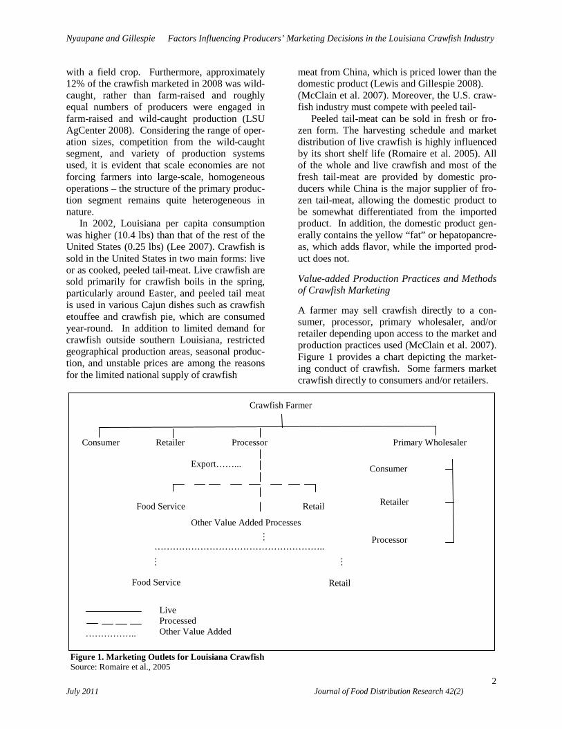
Peeled tail-meat can be sold in fresh or fro-zen form. The harvesting schedule and market distribution of live crawfish is highly influenced by its short shelf life (Romaire et al. 2005). All of the whole and live crawfish and most of the fresh tail-meat are provided by domestic pro-ducers while China is the major supplier of fro-zen tail-meat, allowing the domestic product to be somewhat differentiated from the imported product. In addition, the domestic product gen-erally contains the yellow “fat” or hepatopancre-as, which adds flavor, while the imported prod-uct does not. Value-added Production Practices and Methods of Crawfish Marketing A farmer may sell crawfish directly to a con-sumer, processor, primary wholesaler, and/or retailer depending upon access to the market and production practices used (McClain et al. 2007). Figure 1 provides a chart depicting the market-ing conduct of crawfish. Some farmers market crawfish directly to consumers and/or retailers.
Figure 1. Marketing Outlets for Louisiana Crawfish Source: Romaire et al., 2005
Crawfish Farmer
Export……...
Consumer Retailer Processor Primary Wholesaler
Consumer
Retailer
Processor
Retail Food Service
Other Value Added Processes
…
Retail Food Service
…
………………………………………………..
…
Live Processed Other Value Added ……………..
Crawfish Farmer

Nyaupane and Gillespie Factors Influencing Producers’ Marketing Decisions in the Louisiana Crawfish Industry
3 July 2011 Journal of Food Distribution Research 42(2)
In some cases, consumers go directly to the farm to purchase crawfish, though this is unlikely to occur to a great extent for larger-scale farmers high transactions costs, as discussed by Coase (1937) and later by Williamson (1990), for the large-scale farmer. Producers may sell directly to retailers, with retailers having an interest in dealing with farmers who can guarantee a con-sistently high quality product.
Farmers may sell to processors, who in turn sell to food service and/or retail firms. Proces-sors often peel some (generally smaller) craw-fish and sell it as cooked, peeled tail meat. Par-tially because of the lower priced tail-meat im-ports from China, a reduction of licensed pro-cessors has resulted; in 1996, Gillespie and Capdeboscq (1996) identified 80 processors for surveying, but by 2004, just over 30 processors were identified for surveying by Gillespie and Lewis (2005); thus, the peeling capacity of the industry has decreased (McClain et al. 2007). Primary wholesalers have docks throughout the major crawfish production area of southern Lou-isiana. Farmers may sell crawfish to these wholesalers or, in some cases, wholesalers arrive at the farm to purchase crawfish. Wholesalers, in turn, re-sell the product to retailers, processors, and/or consumers. The wholesaler is an addi-tional firm in the supply chain, introducing an additional transaction (and thus transaction cost) before the product reaches the final consumer. However, from the farmer’s perspective, trans-action costs may be reduced since the entire day’s catch can be marketed to these local buy-ers rather than perhaps sell to multiple firms that may be located further away (increased transpor-tation costs) and may require additional value-added activities. Likewise, the processor or re-tailer may incur lower transaction costs if he or she can purchase in bulk from the wholesaler rather than from a greater number of individual producers. Though this study is not designed to fully compare the net transaction and other costs associated with each of the marketing alterna-tives, it is important that these costs be recog-nized.
When there is market saturation, size grading is a commonly used practice, allowing uniform-sized crawfish to be distributed to the target marketing unit. Larger crawfish have greater appeal for use in crawfish boils, so consumers
generally purchase large crawfish live, whether directly from the farmer or from a primary wholesaler. Smaller-sized crawfish are general-ly peeled by processors for sale as tail-meat. Usually, grading is done in wholesaler or pro-cessing units by using modified vegetable grad-ers or custom-made graders (Romaire et al. 2005). To enhance the appearance and, thus, market value of the product, external wash with ascorbic or citric acid is sometimes done.
The practice of confining crawfish in water without food supplements for one or two days, termed “purging”, is one of the ways to increase the market value of live crawfish. It helps to clean external mud, debris and excretory prod-ucts from the intestine. An additional cost of 15-25% is expected for purging crawfish (Romaire et al. 2005). Value is added, but increased mor-tality risk is associated with purging (McClain et al. 2007).
In areas where live crawfish is available, there are generally a number of small retail out-lets and restaurants specializing in serving boiled crawfish. When the live crawfish market is saturated, smaller-sized crawfish are pro-cessed for tail-meat production or sold to the processing industry, leaving large crawfish for the live market. Some firms cater boiled craw-fish to parties and festivals using custom boiling rigs (Romaire et al. 2005). Data and Methods The Survey The types of marketing arrangements and value-added activities used in Louisiana crawfish pro-duction are assessed using crawfish producer responses obtained from a mail survey conduct-ed during Fall, 2008, to 770 Louisiana crawfish producers. As discussed by Gillespie and Nyaupane (2010) and Nyaupane and Gillespie (2011), surveyed farmers were on the LSU Ag-ricultural Center mailing list for crawfish news-letters. Dillman’s (1978) Total Design Method was followed for implementing the survey, which was eight pages long. Producers were asked questions about marketing practices, gen-eral production practices, tenancy arrangements, adoption of best management practices and rec-
Nyaupane and Gillespie Factors Influencing Producers’ Marketing Decisions in the Louisiana Crawfish Industry
4 July 2011 Journal of Food Distribution Research 42(2)
ord-keeping systems, demographics, and general farm information.
Four mailings were used. The first, in Sep-tember 2008, included the questionnaire and a letter that was personally addressed and signed; first-class mail was used. Non-responders were sent a postcard reminder approximately 1 ½ weeks later. A second copy of the survey fol-lowed the postcard reminder 1 ½ weeks later. Finally, a second postcard reminder was sent to non-responders 1 ½ weeks after the second sur-vey. Several area aquaculture extension agents and LSU Agricultural Center aquaculture faculty were consulted in developing the survey. All area aquaculture extension agents were informed when it was sent to producers. Announcements were made in the July, 2008, Crawfish News, a newsletter distributed to all known Louisiana crawfish farmers, and at the Louisiana Farm Bu-reau annual meeting in July. Of the 770 surveys sent,, 75 were returned as completed, , 185 were returned with the producer stating he or she did not produce crawfish during the 2007-2008 pro-duction season, and 79 were returned as non-deliverable, for an adjusted response rate of 15%. Though the response rate was lower than hoped for, individuals working closely with the industry were generally “enthusiastic” about the return rate, given past data collection experienc-es with the population. This population has been less likely to participate in government programs since there is no crawfish-specific program, so it has been surveyed less than other farm popula-tions.
To determine sample representativeness, sta-tistics are first compared with those of the 2005 Census of Aquaculture, which reports 605 Loui-siana crawfish farms, 433 of which utilized cropland for production. The average acreage of those utilizing croplandwas 176 acres, which is 35 acres less than our survey average of 211 acres. In contrast, Louisiana Summary, 2008, estimated that, for Louisiana, there were 139 acres of crawfish per farm on 1,320 farms. Lou-isiana Cooperative Extension Service agents were used to estimate numbers of farms and acreage on a parish-by-parish basis for Louisi-ana Summary, 2008. The difference in our sam-ple farm size with the estimated population farm size depends upon whether Louisiana Summary, 2008 or Census numbers are used.
Examining the Census of Aquaculture’s 738 Louisiana freshwater aquaculture farms, of which 605 would be crawfish, 49% of the farm-ers leased land and 54% of the land was leased. Our sample suggests 63% leased land, while 42% of the land was leased. Partially because crawfish is often double-cropped or rotated with rice, land leasing arrangements in crawfish are generally more common than with most aqua-culture enterprises. Thus, the higher percentage of producers leasing land in our sample versus the non-crawfish-specific Census sample is as expected. According to the 2007 Census of Ag-riculture, approximately 42% of all Louisiana farmers had farming as their primary occupation, compared with 56% of crawfish farms from our sample. Our survey average age of crawfish farmers is 54; the 2007 Census average age of all Louisiana farmers was 57. An overall com-parison of our survey sample with Census num-bers suggests our surveyed crawfish farms to be more likely to lease land and 20% larger than the average crawfish farm. Assuming crawfish farmers are typical of all Louisiana farmers, our sample is younger and more likely to list farm-ing as their primary occupation. A number of studies have foundfarm respondents to mail sur-veys to be somewhat larger than non-respondents (e.g., Gillespie et al. 2007).
Farmers were asked to choose any of the four marketing outlets applicable to their scenario. The choices include: “I sell to a processor,” “I sell to a wholesaler,” “I sell to a retailer,” and “I sell directly to consumers”. Following this, they were asked, “Do you, at least sometimes”: “Grade your crawfish prior to selling them?”, “Wash your crawfish prior to selling them?”, “Purge your crawfish prior to selling them?”, and “Own or run a commercial crawfish peeling operation?” The survey also included infor-mation on other crawfish production practices, farm characteristics, and farmer characteristics. Econometric Model Probit models are used to analyze factors influ-encing crawfish producers’ choice of marketing outlet. Marketing outlets (dependent variables) include whether the farmer markets crawfish via processors, wholesalers, retailers, and/or con-sumers. Using the probit model, which assumes

Nyaupane and Gillespie Factors Influencing Producers’ Marketing Decisions in the Louisiana Crawfish Industry
5 July 2011 Journal of Food Distribution Research 42(2)
a normal distribution, the probability of adoption is modeled as shown in Greene (2000):
(1)
Pr( ) ( ) ( ' )'
Y t dt xx
= = =−∞∫1 φ ββ
Φ
where φ(.) denotes the standard normal distribu-tion, (Y=1) suggests the marketing outlet was adopted, and x represents independent variables expected to influence adoption. Marginal effects for continuous variables are estimated as: (2) Marginal effects for dummy variables, d, are estimated as: (3) where x* refers to all variables other than d held at their mean values. Though we originally con-sidered using the multivariate probit model to examine market choice among the four market-ing outlets, similar to Fu et al. (1988) and as-suming correlated error terms for each of the equations, several runs using the model suggest-ed that the sample size was insufficient to sup-port this framework. Since farmers may market their crawfish via multiple outlets, the multino-mial logit would be infeasible due to the result-ant very large number of possible choices: 16.
We proceed by discussing independent vari-ables included in the models. Our “expecta-tions” for variable effects are based primarily on economic theory, industry observations, and previous research. Though observations have been made over a number of years working with the crawfish industry, this represents the first attempt we are aware of to quantify portions of producers using various marketing practices and the types of farmers using them; thus our “ex-pectations” are tested as hypotheses. Independent Variables Farm Size and Diversification. Independent variables include Acres of land used in crawfish production (divided by 1,000 in the regression for computational purposes), a measure of craw-
fish production. Greater production is expected to be associated with sales to the wholesaler and processor market because of buyers’ capacity to purchase in bulk. This lowers transaction costs to the producer as he or she need not enter into separate transactions with multiple buyers. Moreover, processors and wholesalers generally also have grading facilities in cases of oversup-ply.
Percent of farm income from crawfish pro-duction (%FarmCF) shows the degree of spe-cialization of a farm. Percent of household in-come from the farming operation (%HHFarm) allows for analysis of the influence of the farmer’s financial dependence from farm opera-tions on choice of market outlet. Though diversi-fication is sometimes used in marketing studies as a measure of the risk faced by a producer (e.g., Gillespie et al. 2004), in our case, there is no known or hypothesized difference in price risk among the alternatives. However, since marketing direct to consumers or retailers is likely to require additional management on the part of the producer (scheduling, dealing with specific requirements, etc.), it is expected that producers who are more highly specialized in crawfish production will more likely market via those outlets. A farmer who is more economi-cally dependent on agriculture is expected to use more innovative production and marketing prac-tices. Fu et al. (1988) showed a relationship be-tween the number of farm enterprises in which a peanut farmer was involved and market choice. Gillespie et al. (2004) and Davis and Gillespie (2007) found farm size and diversification vari-ables to influence farmer choice of cattle mar-keting and hog market outlets, respectively.
Demographic. Previous marketing studies for other agricultural enterprises (i.e., Gillespie et al. (2004) for beef and Davis and Gillespie (2007) for pork) have examined the influence of pro-ducer Age and education on the adoption of a market outlet. We divide producer education into two categories, one without a high-school degree (NoHighSch), the other having at least a four-year College degree. Though additional education categories were available, they were not included due to statistical non-significance and limited observations for the entire sample. The base category, which includes high school graduates and those with some college, repre-
∂∂
φ β βE Y x
xx
[ | ]( ' )=
Pr[ | , ] Pr[ | , ]* *Y x d Y x d= = − = =1 1 1 0

Nyaupane and Gillespie Factors Influencing Producers’ Marketing Decisions in the Louisiana Crawfish Industry
6 July 2011 Journal of Food Distribution Research 42(2)
sents 63% of the sample. The number of Years a farmer has been farming crawfish is a continu-ous variable in increments of seven years, as defined in Table 1. This variable allows for ex-amination of the impact of experience on market selection.
Production Practices. Two dummy variables, whether the producer Grades and/or Washes crawfish prior to selling, were included to de-termine the impact of premarketing practices on the selection of marketing outlets. Farmers who grade and/or wash crawfish prior to selling are expected to be more likely to sell directly to consumers; most processors have their own grading facilities (Gillespie and Lewis 2005), so grading would not be as important in selling to them. Peeling and purging variables were not included in the model due to there being too few farmers using each for inclusion in the model. The number of Months crawfish are produced annually is also likely to influence marketing options available to farmers. Generally, the early
harvesting season runs from November-January when most of the crawfish are immature, mid- season is February-May, an late season is June- July. The price is generally highest early in the production season (winter and early spring) when the demand is highest, while it decreases in the peak and late seasons when the supplies of other seafood products such as shrimp and crabs increase (Romaire et al. 2005). Results General Overview of the Louisiana Crawfish Industry Table 1 provides a general overview of the Lou-isiana crawfish industry, as provided by the sur-vey responses. The average crawfish farm size is 211 acres of crawfish. Although the mean per-centage of farm income from crawfish and per-centage of household income from farming were found to be in the 20-39% and 40-59% ranges,
Table 1. Variables, Descriptions, and Means
Independent Variables Description Mean
Acres Cts: Number of crawfish acres on the farm, divided by 1,000 0.211
%FarmCF Cts: Percent of farm income from the crawfish operation; 1: 1-19%; 2: 20-39%;
3: 40-59%; 4: 60-79%; 5: 80-100% 2.15
%HHFarm Cts: Percent of household income from the farming operation; 1: 1-19%; 2: 20-
39%; 3: 40-59%; 4: 60-79%; 5: 80-100% 3.03
Age Cts: Farmer’s age; 1: ≤30 years; 2: 31-45 years; 3: 46-60 years; 4: 61-75
years; 5: ≥76 years 3.07
College Dummy: Producer holds a college bachelor’s degree or more = 1 0.30
NoHighSch Dummy: Producer without a high school degree = 1 0.07
Years Cts: Number of years a producer has been farming crawfish; 1: 1-7; 2: 8-14; 3:
15-21; 4: 22-28; 5: 29-35; 6: 36-42; 7: ≥43 3.26
Grade Dummy: Producer grading crawfish prior to selling = 1 0.63
Wash Dummy: Producer washing crawfish prior to selling = 1 0.32
Months Cts: Number of months a producer harvests crawfish 5.60
Note: Two other education categories were (1) High School Diploma / GED and (2) Some College or Technical School. Means for these categories were 0.34 and 0.29, respectively.

Nyaupane and Gillespie Factors Influencing Producers’ Marketing Decisions in the Louisiana Crawfish Industry
7 July 2011 Journal of Food Distribution Research 42(2)
respectively, half of the population responded that their farm income generated from crawfish was <20%, while a range of percentage of household income from farming suggested wide diversity in that measure among farms. It is common for producers to rotate crawfish, rice and soybeans, or double-crop rice with crawfish. Furthermore, a typical producer harvests craw-fish for 5-6 months during the year (mean=5.6 months), leaving time for other production activ-ities during the remaining portion of the year. Of the respondents, 29.3% held college degrees, while only 6.6% did not hold a high school di-ploma. The modal range of age of producers was 46-60 years. The modal years of farming experi-ence was 15-21 years. Farmer Premarketing Operations and Selection of Marketing Outlets Table 2 provides framers’ premarketing practic-es conducted before selling. Most of the
respondents (62.5%) grade their crawfish prior to selling. As mentioned earlier, smaller craw-fish are more often used in tail-meat production, and thus have a possible route to processors. Compared to grading, the percentages of farmers washing (31.8%), purging (4.8%), or peeling (7.7%) prior to selling are lower. The lower in-clination towards purging could be partly due to associated mortality risks and higher fixed cost. A peeling operation is generally conducted manually and would usually be considered a labor-intensive separate enterprise with exten-sive specific associated equipment.
Farmer selection of marketing outlets and their proportions are provided in Table 3. Most of the farmers (64.2%) sold crawfish via whole-sale markets. Percentages of producers selling crawfish directly to consumers, retailers, and processors were 30.3%, 22.7%, and 17.9%, re-spectively.
Table 2. Farmer Use of Value-added Production Practices.
Grade: Do you, at least sometimes, grade your crawfish prior to selling them? Categories Frequency Percentage Yes 45 62.5 No 27 37.5 Total 72 100.0
Wash: Do you, at least sometimes, wash your crawfish prior to selling them? Yes 21 31.8 No 45 68.2 Total 66 100.0
Purge: Do you, at least sometimes, purge your crawfish prior to selling them? Yes 3 4.8 No 60 95.2 Total 63 100.0
Peel: Do you, at least sometimes, own or run a commercial crawfish peeling operation? Yes 5 7.7 No 60 92.3 Total 65 100.0

Nyaupane and Gillespie Factors Influencing Producers’ Marketing Decisions in the Louisiana Crawfish Industry
8July 2011 Journal of Food Distribution Research 42(2)
Table 3. Farmer Selection of Crawfish Marketing Outlets.
Which of the following marketing outlets do you use to sell crawfish? (Please check all that apply.)
Categories Total Responses Frequency Percentage
I sell to a processor 67 12 17.9
I sell to a wholesaler 67 43 64.2
I sell to a retailer 66 15 22.7
I sell directly to consumers 66 20 30.3 Note: A farmer may choose to market in more than one outlet during a production season, thus the sum of these percentages is >100%. Probit Results of Farmers’ Choosing a Marketing Outlet Appendix Table 4 shows the factors affecting farmer choice of a crawfish marketing outlet. Larger farmers were found to be more likely to market via retail outlets, likely the result of their ability to guarantee significant volume to supply those markets, reducing transaction costs to the retailer. An additional 1,000 acres of crawfish increased the probability of the farmer market-ing via retailer by 0.34. As initially expected, farmers with higher portions of their farm in-come from crawfish were more likely to market crawfish direct to consumers: a 20% increase in the percent of farm income derived from craw-fish increased the probability of marketing direct to consumers by 0.10. This specialization in crawfish production affords them the opportuni-ty to market crawfish via an outlet that likely involves higher transaction costs, but potentially higher return if customers are willing to pay higher prices to a farmer whose product is per-ceived to be of higher quality. On the other hand, as expected, those with greater percent-ages of income coming from off-farm sources were more likely to market via wholesalers: a 20% increase in the percent of household in-come derived from the farm increased the prob-ability of marketing via wholesalers by 0.14.
Farmer age was positively associated with selling crawfish to processors, while negatively related to selling to wholesalers: an additional 15 years of age increased the probability of mar-keting via processors by 0.13 and decreased the probability of marketing via wholesalers by 0.16. The reduction in the number of processors over a number of years may partially explain
this result, as older farmers continue to market to processors with whom they have built business relationships over a longer time frame. Farmers with college degrees were more likely to sell their product via wholesalers and less likely to market via processors. Holding a college degree increased the probability of marketing via wholesalers by 0.19, but the marginal effect for processors was non-significant. Those without high school diplomas were inclined towards processors and direct to consumers rather than through the wholesale market.
Producer grading of crawfish also had a posi-tive relationship with the wholesale market, while producers washing crawfish were less likely to sell their product to wholesalers and more likely direct to consumers. Producers who graded their crawfish prior to sale had a 0.34 higher probability of marketing via a wholesaler than producers who did not grade their crawfish. Producers who washed their crawfish prior to sale had a 0.63 higher probability of marketing direct to consumers and a 0.66 lower probability of marketing via wholesalers than producers who did not wash their crawfish. Washing crawfish just after harvesting not only removes external debris, but also improves quality by providing a cleaner looking product, so it is not surprising that washing would be done when marketing direct to the consumer. The whole-saler can sell crawfish to processors, retailers, or direct to consumers, so they may conduct grad-ing and/or washing if not already done by the producers.

Nyaupane and Gillespie Factors Influencing Producers’ Marketing Decisions in the Louisiana Crawfish Industry
9 July 2011 Journal of Food Distribution Research 42(2)
Summary and Conclusions This paper deals with factors associated with crawfish farmers’ use of alternative marketing outlets. We use 2008 survey data from a survey of Louisiana crawfish farmers. Four types of marketing outlets commonly used in the industry are analyzed using probit models. Although a farmer can choose a single outlet or a combina-tion of outlets during a production season, the wholesale market was the most commonly used in the industry. A total of 64.2% of the survey sample was found to sell to wholesalers, 30.3% sold directly to consumers, 22.7% to retailers, and 17.9% to processors; given these numbers do not sum to 100%, we see that 35.1% of farm-ers sold via more than one market type. Under-standing how crawfish are marketed is of im-portance when examining the ways in which an industry can regain its competitiveness in an international market. From an international competitiveness standpoint, one would need to take this the next step and examine the transac-tion costs and market efficiency associated pri-marily with the wholesale market to determine whether appreciable increases in efficiency (re-ductions in the cost of getting crawfish to the final consumer) could be gained.
It was found that 62.5% of producers grade and 31.8% wash crawfish prior to selling. Purg-ing is not frequently done by producers, and few producers are involved in the peeling segment. Increased mortality in purging and high costs associated with peeling operation are likely to be two major reasons for lower adoption of those value-added activities.
Younger farmers with higher percentages of household income from farming, with a college degree, and those who grade and do not wash crawfish are more likely to choose the wholesale market. Scale of operation was the major deter-minant of whether farmers would sell directly to retailers, as larger farmers are the ones who have
the volume required to sell directly to the retail market. Farmers who wash crawfish before sell-ing and have higher percentages of their farm income coming from crawfish are the more like-ly farmers to market direct to consumers. Older, less highly educated farmers were more likely to market direct to processors. As expected, de-mographics, farm characteristics, and pre-market activities significant impacted on market choice.
From working with the crawfish industry over a number of years, we have identified a number of issues that have prevented its growth into a larger, national industry, though the indus-try has had an interest in advancing it as such. Many of these issues are structural, such as sea-sonal production, limited production during the season, lack of extensive mechanization in the peeling sector, and the lack of vertical and/or horizontal coordination through either formal contracting or looser strategic alliances. If, however, the industry is to expand significantly beyond Louisiana’s borders, close attention must be paid to development of an industry structure that can perform such that sufficient volume of consistent quality product can be produced year-round and distributed efficiently outside Louisi-ana. For this to occur, significant attention must be paid to marketing – the existing wholesaler and direct-to-processor outlets are likely to be the best places to begin in sourcing these mar-kets. However, significant attention will need to be paid to increasing market efficiency, such as by lowering transaction costs, as the product will need to compete with other seafood products – what must be exported from Louisiana to other United States regions is peeled tail meat, which China currently dominates due to lower prices. Lower-cost domestic production of that product, which currently benefits from its product differ-entiation (fresh, contains “fat,” and “local”), will also be needed. We see determination of an op-timal marketing structure for crawfish industry expansion as a fruitful area of future research.

July 2011 Journal of Food Distribution Research 42(2) 10
References Boucher, R., and J.M. Gillespie, 2010, “Project-
ed Costs and Returns for Crawfish Produc-tion in Louisiana, 2010.” A.E.A. Information Series No. 271, Louisiana Agricultural Ex-periment Station, Louisiana State University Agricultural Center.
Coase, R.H. 1937. “The Nature of the Firm.” Economica 4:386-405.
Davis, C.G., and J.M. Gillespie. 2007. “Factors Affecting the Selection of Business Ar-rangements by U.S. Hog Farmers.” Review of Agricultural Economics 29,2:331-348.
Dillman, D. 1978. Mail and Telephone Surveys: The Total Design Method. John Wiley and Sons, New York.
Fu, T., J.E. Epperson, J.V. Terza, and S.M. Fletcher. 1988. “Producer Attitudes Toward Peanut Market Alternatives: An Application of Multivariate Probit Joint Estimation.” American Journal of Agricultural Economics 70,4:910-918.
Gillespie, J., A. Basarir, and A. Schupp. 2004. “Beef Producer Choice in Cattle Marketing.” Journal of Agribusiness 22,2:149-161.
Gillespie, J., and M. Capdeboscq. 1996. “Factors to Be Considered in the Crawfish Peeling Machine Development Decision.” D.A.E. Research Report No. 705, Dept. of Agricul-tural Economics and Agribusiness, Louisiana State University Agricultural Center.
Gillespie, J., S. Kim, and K. Paudel. 2007. “Why Don’t Producers Adopt Best Management Practices? An Analysis of the Beef Cattle Industry.” Agricultural Economics 36,1: 89-102.
Gillespie, J.M., and D. Lewis. 2005. “Crawfish Processor Preferences for a Crawfish Peeling Machine.” Bulletin 885, Louisiana State University, Agricultural Center.
Gillespie, J.M., and N. Nyaupane. 2010. “Ten-ancy Arrangements Used by Louisiana Craw-fish Producers.” Aquaculture Economics and Management 14,3:202-217.
Greene, W.H. 2000. Econometric Analysis, 4th Edition. Prentice-Hall, Upper Saddle River, New Jersey.
Lee, Y. 2007. “Analysis of the Impact of Fish Imports on Domestic Crawfish Prices and Economic Welfare Using Inverse Demand Systems.” Ph.D. Dissertation, Louisiana State University.
Lewis, D., and J. Gillespie. 2008. “Processor Willingness to Adopt a Crawfish Peeling Machine: An Application of Technology Adoption Under Uncertainty.” Journal of Agricultural and Applied Economics 40,1:369-383.
Louisiana State University Agricultural Center. 2008. “Louisiana Summary, Agricultural & Natural Resources, 2008.” Louisiana Coop-erative and Extension Service, Louisiana State University Agricultural Center.
McClain, W.R., R.P. Romaire, C.G. Lutz, and M.G. Shirley. 2007. “Louisiana Crawfish Production Manual.” Publication 2637, Loui-siana State University Agricultural Center.
Nyaupane, N., and J. Gillespie. 2011. “Louisi-ana Crawfish Farmer Adoption of Best Man-agement Practices.” Journal of Soil and Wa-ter Conservation 66,1:61-70.
Romaire, Robert P., W. Ray McClain, Mark G. Shirley and C. Greg Lutz. 2005. “Crawfish Aquaculture – Marketing.” Southern Region-al Aquaculture Center publication number 2402, Louisiana State University Agricultural Center.
Williamson, O.E. 1990. “Transaction Cost Eco-nomics: The Governance of Contractual Re-lations.” In Industrial Organization. Edward Elgar Publishing, Limited, Brookfield, Ver-mont, 233-261.

Nyaupane and Gillespie Factors Influencing Producers’ Marketing Decisions in the Louisiana Crawfish Industry
11July 2011 Journal of Food Distribution Research 42(2)
T
able
4: P
robi
t Res
ults
of M
arke
ting
Out
let A
naly
sis.
Proc
esso
rs
Who
lesa
lers
R
etai
lers
C
onsu
mer
s C
oeff
icie
nt
(Rob
ust
Std.
Er
ror)
M
arg.
Eff
ect
Coe
ffic
ient
(R
obus
t St
d.
Erro
r)
Mar
g. E
ffec
t C
oeff
icie
nt
(Rob
ust
Std.
Er
ror)
M
arg.
Eff
ect
Coe
ffic
ient
(R
obus
t St
d.
Erro
r)
Mar
g. E
ffec
t
Acre
s -0
.249
8 (0
.945
5)
-0
.025
4
-0
.398
6 (0
.974
5)
-0
.078
9
1.
1965
(0
.624
2)
* 0.
3385
* 0.
1028
(0
.515
8)
0.
0319
%Fa
rmC
F 0.
1004
(0
.275
4)
0.
0102
0.
0860
(0
.215
4)
0.
0170
-0
.264
2 (0
.191
8)
-0
.074
8
0.
3067
(0
.175
2)
* 0.
0951
*
%H
HFa
rm
0.23
12
(0.1
674)
0.02
35
0.
6900
(0
.196
0)
***
0.13
65
**
* -0
.302
9 (0
.208
0)
-0
.085
7
-0
.146
1 (0
.151
4)
-0
.045
3
Age
1.24
20
(0.5
234)
**
0.
1264
**
-0.8
132
(0.4
563)
*
-0.1
609
*
0.25
08
(0.3
844)
0.07
10
0.25
35
(0.3
662)
0.07
86
Col
lege
-1
.051
9 (0
.614
5)
* -0
.090
4
1.
1558
(0
.586
3)
**
0.19
25
*
0.06
23
(0.5
765)
0.01
77
-0.1
647
(0.5
205)
-0.0
502
NoH
ighS
ch
1.83
91
(1.0
811)
*
0.50
18
-2.4
214
(0.8
589)
**
* -0
.772
7
***
1.86
46
(0.9
475)
**
0.
6439
***
Year
s -0
.080
1 (0
.142
8)
-0
.008
2
0.
0887
(0
.162
2)
0.
0176
0.
0348
(0
.156
9)
0.
0099
0.
0377
(0
.133
8)
0.
0117
Gra
de
-0.9
328
(0.6
333)
-0.1
132
1.47
59
(0.5
736)
**
* 0.
3373
**
0.37
82
(0.3
998)
0.10
42
-0.4
690
(0.5
073)
-0.1
492
Was
h 0.
2365
(0
.804
5)
0.
0262
-2
.382
7 (0
.887
9)
***
-0.6
626
**
* 0.
6413
(0
.798
2)
0.
1974
1.
9029
(0
.646
2)
***
0.63
36
**
*
Mon
ths
-0.0
891
(0.2
906)
-0.0
091
0.27
60
(0.2
344)
0.05
46
-0.1
181
(0.2
465)
-0.0
334
-0.0
946
(0.1
833)
-0.0
293
Con
stan
t -4
.679
1 (1
.541
5)
-1
.014
2 (1
.576
1)
-0
.188
6 (1
.564
0)
-1
.605
6 (1
.296
9)
Obs
. 48
48
45
47
Ps
eudo
R2
0.24
17
0.
4033
0.16
20
0.
2921
Not
es: *
** in
dica
tes t
he v
aria
ble
is si
gnifi
cant
at t
he 0
.01
leve
l; **
indi
cate
s the
var
iabl
e is
sign
ifica
nt a
t the
0.0
5 le
vel;
*ind
icat
es th
e va
riabl
e is
sign
ifica
nt a
t the
0.
10
App
endi
x

12
Brand Premiums in the U.S. Beef Industry
Steve Martinez
The U.S. beef industry has experienced considerable reductions in beef demand over the past 30 years. One possible
factor in declining beef demand is lack of progress in the development of consistent, high-quality branded beef
products. This article uses Nielsen Homescan data and hedonic models to estimate the value that U.S. consumers
place on various beef attributes, including brand.
Beef demand indexes suggest a greater long-
term decline in beef demand compared to other
meat products. The beef demand index involves
calculating the real beef price that we would ex-
pect to observe if beef demand was consistent
with demand in the base year. This is compared
to the real beef price actually observed to indi-
cate changes in underlying beef demand. A beef
demand index value of 55 in 2006 (1980=100)
suggests beef retail prices were 45 percent lower
in 2006 than they would have been if beef de-
mand was at its 1980 level (Tonsor, 2010). That
is, beef demand fell by 45 percent since 1980.
This compares to a pork demand index of 65,
which suggests that pork demand fell by 35 per-
cent over the same period. Along with changing
consumer preferences and heightened health
consciousness, poor quality assurance has been
offered as one reason for the decline in beef de-
mand (Brester, Schroeder, and Mintert, 1997;
Ferrior and Lamb, 2007; Purcell, 2002; Purcell
and Hudson, 2003). Marketing of differentiated
beef products may be hampered by the fact that
beef quality is unknown when cattle are sold,
and quality variation related to genetics makes it
difficult to establish branded products (Bailey,
2007; Ward, 1997; Ward, undated).
According to Ward (1997), one of the biggest
obstacles to greater vertical coordination in the
beef sector is difficulty in controlling quantity,
quality, and consistency. Large capital require-
ments are involved in controlling a large number
of small and geographically dispersed cow-calf
producers. Measuring and controlling quality
and end-product consistency also is a problem
Martinez is with the Economic Research Service at the U.S.
Department of Agriculture in Washington D.C. The views
expressed here are those of the author and cannot be at-
tributed to the Economic Research Service or the U.S. De-
partment of Agriculture.
because of several factors, including the wide
genetic base, longer production cycle required to
quickly change the genetic base, greater number
of production stages, and lack of economical
measuring technology.1
Brand premiums can provide the necessary
incentives for sourcing cattle of higher quality
and consistency, and they can provide opportu-
nities for increasing revenues to be allocated
across the supply chain (i.e., producers, proces-
sors, distributors). Yet, limited research exists on
how consumers value branded beef products.
Parcell and Schroeder (2007), using a national
survey of about 2,000 households from 1992 to
2000, found price premiums for branded roasts
and steaks (mostly Certified Angus Beef®)
compared to store brands, but not for branded
ground beef. Based on data collected from gro-
cery stores in three metropolitan areas from Ju-
ly-August 2006, Ward et al. (2008b) found price
premiums for branded roast/steak and ground
beef compared to unbranded/generic beef. In this
study, we conduct a hedonic analysis to estimate
implicit prices of branded beef using more re-
cent data than Parcell and Schroeder (2007) and,
unlike Ward et al. (2008b), uses scanner panel
data that is national in scope from a panel of rep-
resentative U.S. households.
Role of Brands
Consumers may be willing to pay a premium for
branded products because branding can help to
overcome problems that have limited beef sales.
Branding provides a means for signaling quality.
Brands can help consumers process, interpret,
and store large quantities of information about
products. As a source of information, brands
1Other factors noted by Ward include capital requirements,
and management skills required to manage many, small,
and geographically dispersed cattle operations through
several production stages.

Martinez Brand Premiums in the U.S. Beef Industry
13
July 2011 Journal of Food Distribution Research 42(2)
serve as substitutes for the time and skills re-
quired for evaluating product quality (Jin, Zil-
berman, and Heiman, 2008).
Brands are particularly important in cases
where information necessary for obtaining an
objective determination of quality is limited at
the time of purchase, as with experience and
credence attributes (Jin, Zilberman, and Heiman,
2008).2 For unprocessed beef, there may be only
minor detectable quality differences at the store
for products within the same category. Yet,
considerable biological variation may exist,
which results in different quality experiences.
This situation compels consumers to search for
other informational cues in the evaluation of
unprocessed beef at the store. Branded beef has
been shown to serve as the predominant cue for
expected eating and health quality (Bredahl,
2003).
When companies develop products with
unique quality attributes, these products are gen-
erally sold as branded products. Producers of
branded products must support their brands by
investing in quality control because perceived
average quality levels and quality variation can
affect premiums paid for branded products. Per-
ceived quality is based on consistency of product
characteristics, such as eating satisfaction and
safety, from one purchase to the next. Brands
can increase consumers‟ confidence regarding
the purchase decision because of past experience
with the product or familiarity with the brand
and its characteristics.
Consumers may be willing to pay a higher
price for branded products because of reduced
search costs, and companies‟ commitment to
quality to prevent losses in brand name invest-
ments and reputation (Fernandez-Barcala and
Gonzalez-Diaz, 2006). In addition, if a brand is
well positioned with respect to a key attribute,
such as tenderness, competitors will find it diffi-
2Experience attributes are those that are costly to measure
by the consumer prior to purchase, but are easily measured
as the product is consumed (e.g., tenderness, taste). Cre-
dence attributes are those that are difficult to measure be-
fore and after purchasing (organic, natural). On the other
hand, search attributes have a low cost of measuring at the
time the purchase (e.g., color, visible fat). For search at-
tributes, additional information provided by the brand is
less likely to have significant value to the buyer (Pearson,
2003).
cult to differentiate their products based on the
same attribute.
Nielsen Homescan Data
This research uses Nielsen Homescan data for
household purchases in calendar years 2004 and
2005. Consumer panel participants were selected
based on demographic and geographic targets to
match the U.S. population as closely as possible.
The nationally representative panel contains
about 8,000 households per year who participat-
ed for at least ten months. These households
recorded both their non-UPC-coded random-
weight and UPC-coded purchases after each
shopping trip using an electronic scanner located
at their home.3 For non-UPC-coded random-
weight products, information is manually rec-
orded using Nielsen‟s “Category Code Book For
Non-UPC Barcoded Items.”4 The individual
household food purchase data contains infor-
mation on expenditures, quantities and date pur-
chased, package size, number of units, price
promotions (coupons, store features, and other
deals), and brand. The data also contain demo-
graphic information for each household, such as
geographic location, income, race, household
size, education, and age.
Nielsen Homescan data include brand infor-
mation for fresh, frozen, and precooked ground
beef, steak, roast, and other beef cuts (e.g., beef
for stew, ribs, liver, brisket).5 Table 1 summariz-
es Nielsen‟s brand classifications for non-UPC
random-weight and UPC-coded beef. Non-UPC
coded random-weight beef has three broad brand
descriptors: an actual brand name (e.g., Cole-
man Natural Beef, Swift); an “all other brands
category;” and “no brand.” UPC-coded beef cuts
have four basic brand descriptors. These include
3Random-weight items are products that do not have a
standard weight. 4The category code book is used for products with non-
UPC barcodes and those without any barcodes. Panelists
are instructed to first scan non-UPC barcoded items before
using the code book. 5Our analysis excludes further processed products, includ-
ing sausages and hotdogs, canned meat, jerky, meat snacks,
frozen entrees, lunch meat, refrigerated and frozen ready-
made sandwiches, sandwich spreads, and soups.

Martinez Brand Premiums in the U.S. Beef Industry
14
July 2011 Journal of Food Distribution Research 42(2)
the actual brand name; “CTL BR,” which are
private label (i.e., store brand) products (e.g.,
Giant or Safeway's Rancher's Reserve brand);6 a
company name followed by “NBL” (no brand
label) (e.g., Tyson Fresh Meats---NBL); and
“NBL---no company listed.” The “NBL- no
company listed” identifier means that the item
did not have a label identifying the supplier. For
random-weight beef, Nielsen considers private
label products to be unbranded if the store name
is the brand.7
Extent of Beef Branding
In this section, we use household projection fac-
tors (weights) contained in the Homescan data to
aggregate household purchase data, which we
then use to describe branded beef purchases in
the United States. Each household is assigned a
6Private label or store-branded beef is exclusively devel-
oped, manufactured, and produced for a retailer. According
to the Private Label Manufacturers Association, the brand
can be the store‟s own name or a name created exclusively
by that store. 7Information on the frequency distribution of purchases by
type of brand, including those that have no brand present,
are included table 3 for non-UPC random weight beef and
table 5 for UPC-coded beef.
projection factor based on its demographics to
make aggregate statistics representative at the
national level. Each household is weighted by its
projection factor according to its representation
in the U.S. population based on U.S. Census da-
ta. A weighted quantity and expenditure is cal-
culated for each recorded transaction, which can
then be aggregated over all household transac-
tions to obtain totals that are representative of
national purchases. Nielsen recalculates the
weights each year to maintain consistency with
Census updates.8
Due to differences in brand classifications, as
discussed earlier, we used Nielsen Homescan
data to conduct separate analyses of non-UPC-
coded random-weight beef, which accounted for
87 percent of beef poundage purchased in 2005,
and UPC-coded beef. Consumers spent $3.1 bil-
lion on 1 billion pounds of random-weight
branded beef cuts in 2005, or 25 percent of ran-
dom-weight beef pounds purchased. In compar-
ison, branded products accounted for 63 percent
of random-weight chicken pounds purchased
and 46 percent of random-weight pork pounds
purchased in 2005 (Nielsen Homescan data).
For random-weight beef, we focus on ground
beef, steaks, and roasts, which accounted for 85
8More details on the projection factors can be found in
Harris (2005).
Table 1. Classification of Branded Beef in the Nielsen Homescan Data,
Calendar Years 2004 - 2005 Product modules Brand descriptors Branded?
Non-UPC coded random-weight beef
No brand (includes those cuts branded with the store name)1 No
Brand name (e.g., Sterling Silver, Swift, Store-specific brands
that are not the store name)
Yes
All other brands
Yes
UPC-coded beef
Brand name
Yes
CTL BR (all private label/store brands)2
Yes
NBL-no company listed
No
Supplier name-NBL (e.g., Tyson Fresh Meats-NBL)3
No
1According to the Nielsen code book for non-UPC barcoded items, panelists are instructed to type the brand name into the
scanner as it appears on the package label. If there is no brand name on the package, or if the store‟s name is the brand name,
they are asked to press the “no” key on their scanner. Hence, private label products where the brand name is the store name
(e.g., Kroger or Giant) are included in the “no brand” category, there is no way to segregate these brands from the category. 2Includes all private label products, including those brands where the brand is the name of the store. 3These products identify the supplier, but the company name is not the brand name.

Martinez Brand Premiums in the U.S. Beef Industry
15
July 2011 Journal of Food Distribution Research 42(2)
percent of random-weight beef pounds pur-
chased in 2005, the latest year in our sample
(Nielsen Homescan data). Twenty-two percent
of random weight ground beef carried a brand,
compared to 25 percent of steaks and roasts. A
smaller percentage of branded ground beef may
be due to the fact that the degree of leanness is
the primary factor that distinguishes ground beef
(Parcell and Schroeder, 2007). In 2005, 87 per-
cent of ground beef purchased carried a leanness
specification, and accounted for 95 percent of all
beef with information on leanness (Nielsen
Homescan data).
In 2005, the percentage of beef purchased
through some type of price promotion, including
store and manufacturer coupons, store features,
and other deals, was slightly higher for branded
versus unbranded beef; 43 percent compared to
41 percent (Nielsen Homescan data). Price pro-
motions and competition between store types
can create incentives to improve product quality
and consistency of branded products. Price pro-
motions provide a quick and measureable means
of increasing sales. However, promotions that
simply offer a price discount may also cheapen
the value of a brand, harm the brand image, and
reduce the likelihood of future brand purchases
(Aaker, 1991; Gedenk and Neslin, 1999). In the
long term, price promotions can increase sales,
but should be used in conjunction with adver-
tisements and product improvements to increase
the likelihood of future brand purchases
(Gedenk and Neslin, 1999).
One of the most important developments in
the food retail sector has been the growth in food
sales by stores that did not traditionally sell
many food items, especially wholesale clubs and
supercenters. Homescan Panel data distinguishes
stores by store type. The share of branded ran-
dom-weight beef purchased at wholesale clubs
was highest compared to grocery stores and
supercenters. In 2005, 34 percent of random
weight beef purchased at wholesale clubs carried
a brand label, compared to 23 percent at grocery
stores and 12 percent at supercenters.
Beef that is UPC-coded allows consumers to
select beef cuts quicker because they don‟t have
to search through packages to find the preferred
weight or price. UPC-coded items also facilitate
tracking of product movement by the supplier,
and tracing of product by the buyer back to the
supplier. In this study, we focused on UPC-
coded ground beef, which accounted for 96 per-
cent of UPC-coded purchases in 2005.9 Branded
UPC-coded ground beef purchased as a share of
total UPC-coded ground beef was 69 percent in
2005. Grocery stores and supercenters account-
ed for 82 percent of UPC-coded ground beef
purchases, and 86 percent of this beef was
branded at grocery stores compared to 31 per-
cent at supercenters.
Hedonic Regression Model Results
To examine price premiums associated with
specific beef brands, we estimated a hedonic
regression model using sample data on house-
hold purchases contained in the Nielsen
Homescan data for 2004 and 2005. The hedonic
price model assumes that consumers derive utili-
ty from the characteristics of goods rather than
the goods themselves (Ladd and Suvannunt,
1976; Unnevehr and Bard, 1993). Price differ-
ences are assumed to be due to differences in
product attributes which include intrinsic and
extrinsic quality attributes (Parcell and Schroed-
er, 2007; Pearson, 2003). Intrinsic attributes are
those associated with the actual characteristics
of the product, such as fat content, taste, smell,
and color. Extrinsic attributes relate to promo-
tional or informational characteristics that can
also affect consumer choice, including brand.
We also assume that prices may vary by location
of the household, as well as month and year of
purchase.
To estimate price differences between brand-
ed and unbranded beef, we first classified brands
into specific categories. There is no consensus in
the literature on how to categorize brands. Ward
et al. (2008b) identified four specific types of
brands including special, program, store, and all
other brands, along with an “unbranded” catego-
ry. Special brands were those that carried a label
identifying production practices, such as “all
natural.” Program brands were breed specific,
such as Certified Angus Beef. In addition to
store brands and unbranded beef, Schulz et al.
(2010) classified beef into three brand categories
9Steak accounted for most of the remainder, and nearly all
of it was branded.

Martinez Brand Premiums in the U.S. Beef Industry
16
July 2011 Journal of Food Distribution Research 42(2)
based on the range of distribution. A national
brand is distributed nation-wide and is con-
trolled by the company that owns the brand. A
local private brand is distributed locally and is
privately owned and controlled by a small com-
pany. A regional private brand is distributed re-
gionally and is owned and controlled by a pri-
vate company. In addition to store brands, the
National Cattlemen‟s Beef Association (NCBA)
(undated) identified two other types of branding
programs, similar to those defined by Ward et al.
(2008). A breed-specific branded beef program
selects beef from a specific breed. Company-
specific branded beef is not breed specific, but
includes other criteria, such as premium grade,
no antibiotics or hormones, source verified, or
grass-fed. Examples include Sterling Silver™
Beef or Maverick Ranch.
In this study, we combine the brand nomen-
clature described above to classify beef into six
categories: 1) breed-specific/program brands, 2)
company-specific/special brands, 3) private la-
bel/store brands, 4) national brands, 5) all other
brands, 6) unbranded beef. Private label brands
can be further classified into three general types:
generic, no frills, low-priced products; national-
brand equivalents (i.e., copies the national
brands, but sold at lower price); and premium,
value-added private label that is priced near or
above the brand leader (Rivkin, 2006; Forgrieve,
2007). National brands are established brands
that do not fall into any of the other brand cate-
gories, such as Hormel and Tyson.
Random-Weight Beef
Table 2 contains summary statistics for the con-
tinuous variables and table 3 contains the fre-
quency distribution for all discrete variables
used to estimate the random-weight hedonic
models in this study. For random-weight beef,
Nielsen data contain 12 brand names of sub-
stance (i.e., those with at least 15 observations
per year, and 250,000 pounds purchased annual-
ly based on weighted and aggregated quantities
across households to obtain a nationally repre-
sentative total), including six national brands,
four private label brands, a company-specific
brand, and a breed-specific brand. National
brands were less prevalent for ground beef and
roast, while the other types of brands were well
represented across each cut. To protect proprie-
tary information, we do not divulge the names of
specific brands.
The following equation was estimated for
each of the three leading cuts of beef:
(1) P = α + β1YEAR + β2SIZE + β3SIZESQ
+ β4ProductForm +
4
1i
ii omotiondPr
+
3
1i
iStoreTypesf i +
3
1i
ii gionrRe
+
3
1i
ii nPercentLeal +
2
1i
iiSteakCutq
+
13
1i
iiBrandb +
11
1i
iiMonthm + μ
where P is price per pound,10
the Brandi„s are
dummies for the 12 brand names of substance
and an “all other brands” category (base=no
brand), SIZE is the unit weight of the package
purchased by the household, SIZESQ is unit
weight squared, the Promotioni„s are dummy
variables that account for the four promotion
categories (store feature, store coupon, manufac-
turer coupon, other deal, base=no deal), the Sto-
reTypesi„s are dummies for three store types
(supercenter, warehouse club, other, base= gro-
cery stores), the Regioni„s are dummies for three
of the four regions (South, West, Central,
base=East), the PercentLeani„s are dummies for
percent lean classifications of ground beef (less
than 80%, 80% to 89%, 90% or greater,
base=lean not specified), ProductForm is equal
to 1 if ground beef is purchased as preformed
patties and is equal to 0 if it is purchased in bulk
form, the Monthi„s are monthly dummy varia-
bles (base=December), and μ is a random error
term. A dummy variable, YEAR, takes the val-
ue 1 for purchases in 2005, and 0 for those in
2004. The SteakCuti„s are dummies for quality
of steak cut (Medium, High, base=Low) among
fifteen cuts of steak identified in the data.
10Beef prices were imputed by dividing expenditures (in-
corporating any price promotions that may have accompa-
nied the purchase, such as store coupons) by the amount
purchased.
Martinez Brand Premiums in the U.S. Beef Industry
17
July 2011 Journal of Food Distribution Research 42(2)
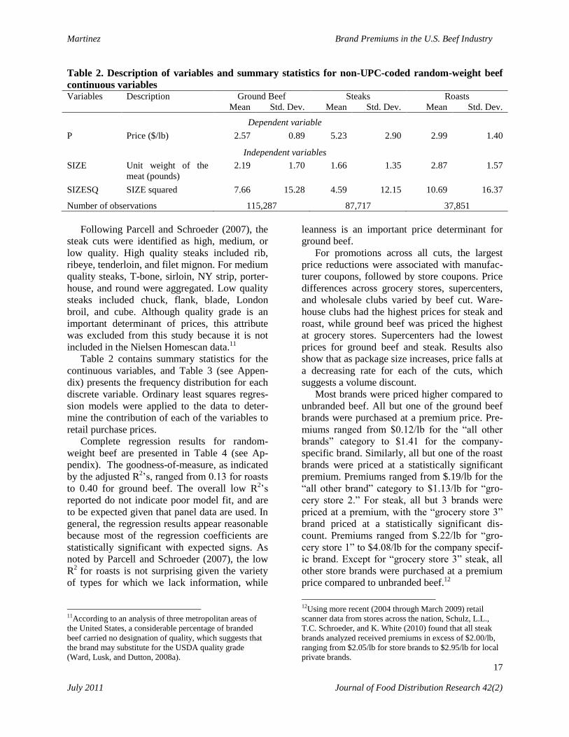
Table 2. Description of variables and summary statistics for non-UPC-coded random-weight beef
continuous variables Variables Description Ground Beef Steaks Roasts
Mean Std. Dev. Mean Std. Dev. Mean Std. Dev.
Dependent variable
P Price ($/lb) 2.57 0.89 5.23 2.90 2.99 1.40
Independent variables
SIZE Unit weight of the
meat (pounds)
2.19 1.70 1.66 1.35 2.87 1.57
SIZESQ SIZE squared 7.66 15.28 4.59 12.15 10.69 16.37
Number of observations 115,287 87,717 37,851
Following Parcell and Schroeder (2007), the
steak cuts were identified as high, medium, or
low quality. High quality steaks included rib,
ribeye, tenderloin, and filet mignon. For medium
quality steaks, T-bone, sirloin, NY strip, porter-
house, and round were aggregated. Low quality
steaks included chuck, flank, blade, London
broil, and cube. Although quality grade is an
important determinant of prices, this attribute
was excluded from this study because it is not
included in the Nielsen Homescan data.11
Table 2 contains summary statistics for the
continuous variables, and Table 3 (see Appen-
dix) presents the frequency distribution for each
discrete variable. Ordinary least squares regres-
sion models were applied to the data to deter-
mine the contribution of each of the variables to
retail purchase prices.
Complete regression results for random-
weight beef are presented in Table 4 (see Ap-
pendix). The goodness-of-measure, as indicated
by the adjusted R2‟s, ranged from 0.13 for roasts
to 0.40 for ground beef. The overall low R2‟s
reported do not indicate poor model fit, and are
to be expected given that panel data are used. In
general, the regression results appear reasonable
because most of the regression coefficients are
statistically significant with expected signs. As
noted by Parcell and Schroeder (2007), the low
R2
for roasts is not surprising given the variety
of types for which we lack information, while
11According to an analysis of three metropolitan areas of
the United States, a considerable percentage of branded
beef carried no designation of quality, which suggests that
the brand may substitute for the USDA quality grade
(Ward, Lusk, and Dutton, 2008a).
leanness is an important price determinant for
ground beef.
For promotions across all cuts, the largest
price reductions were associated with manufac-
turer coupons, followed by store coupons. Price
differences across grocery stores, supercenters,
and wholesale clubs varied by beef cut. Ware-
house clubs had the highest prices for steak and
roast, while ground beef was priced the highest
at grocery stores. Supercenters had the lowest
prices for ground beef and steak. Results also
show that as package size increases, price falls at
a decreasing rate for each of the cuts, which
suggests a volume discount.
Most brands were priced higher compared to
unbranded beef. All but one of the ground beef
brands were purchased at a premium price. Pre-
miums ranged from $0.12/lb for the “all other
brands” category to $1.41 for the company-
specific brand. Similarly, all but one of the roast
brands were priced at a statistically significant
premium. Premiums ranged from $.19/lb for the
“all other brand” category to $1.13/lb for “gro-
cery store 2.” For steak, all but 3 brands were
priced at a premium, with the “grocery store 3”
brand priced at a statistically significant dis-
count. Premiums ranged from $.22/lb for “gro-
cery store 1” to $4.08/lb for the company specif-
ic brand. Except for “grocery store 3” steak, all
other store brands were purchased at a premium
price compared to unbranded beef.12
12Using more recent (2004 through March 2009) retail
scanner data from stores across the nation, Schulz, L.L.,
T.C. Schroeder, and K. White (2010) found that all steak
brands analyzed received premiums in excess of $2.00/lb,
ranging from $2.05/lb for store brands to $2.95/lb for local
private brands.

Martinez Brand Premiums in the U.S. Beef Industry
18
July 2011 Journal of Food Distribution Research 42(2)
The highest premiums were found for brands
produced through alternative pricing and mar-
keting arrangements. For the company-specific
branded ground beef and steak, a family-owned
beef company produces the source-verified lines
of natural, organic, and grass-fed beef, using
enhanced food safety practices. It was one of
the first branded beef systems to pay producers
according to the true value of each animal, rather
than paying an average price for the entire pen
of cattle.13
The company uses contracts with
feedlots and ranches where the cattle are born.14
Among the five national steak brands, three
were purchased at a statistically significant pre-
mium compared to unbranded steak, with sizea-
ble differences across brands. National brands 3
and 6 had relatively high premiums. To qualify
for national brand 3‟s program, producers must
choose genetics that provide non-black hided
cattle with specific quality and yield grade re-
quirements.15
Cattle supplies are obtained from
an alliance between the company, a breed asso-
ciation, and a marketing services provider. Stra-
tegic alliances enable firms to share risks and
benefits from mutually identified objectives,
while allowing partners to maintain their inde-
pendence (Brocklebank and Hobbs, 2004).
The company that produces national brand 6
was purchased prior to 2004 by a producer-
owned “new generation” cooperative. New gen-
eration cooperatives are distinguished from tra-
ditional cooperatives because they add value to a
raw agricultural product through further pro-
cessing, thereby allowing producers to capture a
larger portion of downstream value. Members
of the branded beef company purchase or lease
shares that entitle them to deliver one head of
13When compensation is based on average price, differ-
ences in quality among cattle within the pen are not consid-
ered, which quells economic incentives to produce higher
quality cattle. High-quality cattle will be under compen-
sated, while low-quality cattle will be over compensated. 14The company also has diversified its product offerings to
include buffalo and chicken. A strong brand with respect
to perceived quality can be exploited by extending the
brand to other product categories (Aaker, 1991). 15A quality grade is a composite evaluation of factors that
affect palatability of meat (tenderness, juiciness, and fla-
vor). Basic quality grades include Prime, Choice, and Se-
lect, where Prime represents the highest quality and Select
represents the lowest. Yield grades reflect the amount of
boneless, closely trimmed retail cuts.
cattle for each share. Producers are rewarded for
delivering high quality cattle based on a grid
pricing system that prices individual cattle based
on quality and yield grade.16
The breed-specific brand premium also
ranked among the highest for ground beef,
steaks, and roasts. Breed-specific brands are of-
ten organized as a brand licensing program (li-
censed by the breed organization) that typically
requires that cattle meet certain genetic require-
ments (often breed-based), and uses the breed as
a proxy for quality (Brocklebank and Hobbs,
2004). They tend to involve loose contract ar-
rangements with the only requirements being
that participants are certified to sell beef under
the program name and that the breed of cattle
can be verified. Producers may choose to sell all
or no cattle through the program, and premiums
are generally based on yield or quality. Less
formal marketing arrangements are possible be-
cause of the broad requirements and focus on
breed, which can be easily observed.
Regarding ground beef leanness and product
form, and quality of the steak cut, ground beef
that was 90 percent lean or greater commanded a
premium of $0.68/lb compared to ground beef
without a leanness specification. Ground beef
that was 80 to 89 percent lean received a premi-
um of $0.12/lb, while the less than 80 percent
lean category was discounted by $0.16/lb com-
pared to no leanness specification.17
Preformed
ground beef patties were purchased at a premi-
um of $0.26/lb compared to bulk ground beef.
This may reflect further processing costs associ-
ated with the beef patties or the convenience
preferred by time-pressed consumers. For steak,
as expected, the higher quality cuts received the
largest premiums.
Prices also varied by geographic location and
season. All cuts were priced lower in the Cen-
tral region, and highest in the East or West.
Prices were lowest from January to June for
16With grid pricing, the price paid for an animal depends on
various quality attributes, in addition to weight (Hueth and
Lawrence, 2006). This differs from traditional spot markets
where price is based on live or carcass weight, with no
explicit adjustments for quality. 17These results are consistent with previous studies that
found a price premium for leaner ground beef (Brester,
Lhermite, Goodwin, and Hunt, 1993; Parcell and Schroed-
er, 2007; Ward, Lusk, and Dutton, 2008b).

Martinez Brand Premiums in the U.S. Beef Industry
19
July 2011 Journal of Food Distribution Research 42(2)
ground beef, and February to October for roast,
while steak exhibited much more price variation
across months.
UPC-Coded Ground Beef
Table 5 (see Appendix) contains summary statis-
tics and frequency distributions for UPC-coded
ground beef data used to estimate the hedonic
price model (equation 1). The brand names ex-
amined include those associated with the top 20
brands in purchase volume, along with the pri-
vate label category in 2004 and 2005.18
In addi-
tion to ground beef purchased as preformed pat-
ties, the UPC-coded data also provides infor-
mation on ground beef purchased in chub pack-
ages.
Regression results are presented in Table 6
(see Appendix). The model explains more of the
variation in prices compared to random-weight
ground beef, as indicated by the adjusted R2 of
0.56 compared to 0.40 for random-weight beef.
Other than brands, results for most variables
were similar to those found in the non-UPC cod-
ed random-weight ground beef model.
Brand premiums/discounts ranged from -
-$1.06/lb to $1.12/lb. The number of brands and
brand categories priced at a statistically signifi-
cant discount compared to unbranded beef was
nearly equal to the number that received premi-
ums. As with random-weight beef, the highest
premiums were paid for brands produced
through alternative pricing systems and vertical
coordination arrangements, including brand 12
and brand 7. Brand 12 garnered the highest pre-
mium. According to company literature, the line
includes natural beef and beef that is cobranded
with a breed-specific label. The company that
produces cattle for the breed-specific label oper-
ates as a division of a breed association to pro-
duce high quality, tender, and flavorful beef.
The company does not own cattle or beef at any
stage of production or processing. As part of the
program, cattle must comply with certain carcass
specifications, and licenses are sold to proces-
sors, distributors, retailers, and restaurants to
harvest, fabricate, and sell the beef. In May
18In 2005, over 100 UPC-coded beef brand names were
listed in the Nielsen Homescan Panel data, compared to
only 46 non-UPC-coded random-weight brand names.
2010, it was one of 62 programs certified by
USDA inspectors that go beyond requirements
for official USDA grades to facilitate the mar-
keting of branded beef products.
The brand 7 company, which had the second
highest premium of $1.06/lb, produces naturally-
raised, lean beef. Price premiums, relative to the
spot market, are paid for lean, heavily muscled
cattle that are free of antibiotics and added
growth hormones. The beef achieves its lean-
ness through specialized inputs, including the
selection of cattle breeds and a feed program
that includes grazing and natural feeds. Farmers
who produce cattle for the program sign a legal
contract agreeing to adhere to the company's
requirements regarding feed and other manage-
ment. Bonus or discounts apply to the contract
price on an individual carcass basis.
Among those brands receiving the largest
discounts, brand 11 frozen beef patties had the
largest discount of $1.06/lb, followed by brand 2
which was purchased at a $0.87/lb discount. In
2005, brand 2 beef patties were voluntarily re-
called because of possible E. coli contamination.
Following the recall, the brand price was dis-
counted an additional $0.15/lb.19
According to
company literature, the brand 11 company offers
a range of branded products are offered to ap-
peal to different customer preferences, including
one that is targeted to the cost-conscious con-
sumer. Private label brands were priced at a dis-
count of $0.13/lb compared to unbranded beef,
which suggests that these brands are generally
positioned as generic, lower-priced alternatives.
We found discounts for less than 80 percent
lean (-0.28/lb), and higher premiums for leaner
beef ($0.20/lb for 80 to 89 percent lean and
$0.63/lb for 90 percent lean or greater) com-
pared to packages with no leanness specifica-
tion. Premiums were also paid for ground beef
purchased in preformed patty form ($0.34/lb)
and in chub packages ($0.44/lb) compared to
bulk ground beef. The largest price discounts
were found in the South (-$0.08/lb), followed by
the Central region (-$0.03/lb) (relative to the
East). Prices were highest in the West. There
was no statistically significant price difference
19To capture price adjustments following the recall, an
additional dummy variable was added that equals one in the
months following the recall, and zero otherwise.

Martinez Brand Premiums in the U.S. Beef Industry
20
July 2011 Journal of Food Distribution Research 42(2)
between the East and West. Price discounts
were greater at warehouse clubs (-$0.25/lb) than
supercenters (-$0.11/lb) (relative to grocery
stores). Seasonal differences were also found as
prices were statistically significantly lower from
January to June compared to the rest of the year.
For package size, resulting coefficient estimates
were similar to those of random-weight beef,
suggesting volume discounting.
Implications and Conclusions
Nielsen Homescan data were used to estimate
the effect of observable beef product attributes
on retail beef prices. Our results indicate that
beef cuts on sale are significantly less than
nonsale items, and larger package sizes are pur-
chased at a significant discount. Prices also vary
by store format (grocery store, supercenter, or
warehouse club), depending on type of beef cut.
Use of more recent data (after 2007) would al-
low us to examine the effect of the recession on
sales discounts. Steak prices are higher at ware-
house clubs and lower at supercenters, compared
to grocery stores. For roasts, prices are higher at
both warehouse clubs and supercenters com-
pared to grocery stores, while for both random-
weight and UPC-coded ground beef, prices are
highest at grocery stores.
The data were national in scope and collected
over the 2004 and 2005 calendar years. Results
indicate that prices vary by region, with the low-
est prices occurring in the Central region for
random-weight beef. For UPC-coded ground
beef, the lowest prices are found in the South,
but regional differences are smaller than ran-
dom-weight ground beef. Random-weight steaks
and roasts exhibit greater seasonal variation than
both random-weight and UPC-coded ground
beef.
Most random-weight beef brands contained
in the Nielsen Homescan data garner premiums
compared to unbranded products, but premiums
varied widely across brands. For example, for
steak, premiums range from $0.21/lb for a store
brand to $4.15/lb for a brand produced with spe-
cific production protocols, including grass fed
and source verified. There is much greater varia-
tion in brand premiums across specific steak
brands than for the aggregate brand categories
found by Schulz et al. (2010). For most private-
label brands, random-weight beef brands are
purchased at a premium compared to unbranded
beef. Conversely, the UPC-coded ground beef
private label category as a whole is discounted.
UPC-coded ground beef brands are evenly split
between those purchased at a premium and those
purchased at a discount compared to unbranded
beef. This suggests that a considerable number
of these brands target cost-conscious consumers.
While the classification of brand types is re-
stricted by the data source used, efforts to devel-
op common nomenclature would facilitate brand
comparisons across studies.
By evaluating specific brands, we were able
to identify the production protocols used for the
branded products. The highest premiums are
paid for those brands with specific production or
quality requirements. Branding programs receiv-
ing the highest premiums also rely on alternative
marketing arrangements (e.g., alliances, con-
tracts, cooperatives). This suggests that premi-
ums for value-added, branded products may
strengthen incentives for producers and proces-
sors to enter into these arrangements to achieve
the necessary coordination and quality control.
Shifts to alternative marketing arrangements
in the beef industry have led to concerns about
market power, and policy proposals to restrict
the types of marketing arrangements used (An-
derson and Hudson, 2008; Ferrell and Rumley,
2011). The potential role of these arrangements
in facilitating industry efforts to capture premi-
ums associated with consumers‟ willingness to
pay for quality attributes in branded product
lines should also be considered. Less market-
distorting policy alternatives to restrictions on
marketing arrangements may be those that facili-
tate the marketing of value-added, branded
products, such as USDA quality certification
programs.

Martinez Brand Premiums in the U.S. Beef Industry
21
July 2011 Journal of Food Distribution Research 42(2)
References
Aaker, D.A. 1991. Managing Brand Equity:
Capitalizing on the Value of a Brand Name.
New York, NY: The Free Presss.
Anderson, J.D., and D. Hudson. 2008. “Acqui-
sitions and Integration in the Beef Industry.”
Policy Issues, PI2, September, pp. 1-4.
Bailey, D. 2007. “Political Economy of the U.S.
Cattle and Beef Industry: Innovation Adop-
tion and Implications for the Future.” Journal
of Agricultural and Resource Economics,
Vol. 32, pp. 403-416.
Bredahl, L. 2003. “Cue Utilization and Quality
Perception with Regard to Branded Beef.”
Food Quality and Preference, Vol. 15, pp.
65-75.
Brester, G.W., P. Lhermite, B.K. Goodwin, and
M.C. Hunt. 1993. “Quantifying the Effects of
New Product Development: The Case of
Low-Fat Ground Beef.” Journal of Agricul-
tural and Resource Economics, Vol. 18, pp.
539-550.
Brester, G.W., T.C. Schroeder, and J. Mintert.
1997. “Challenges to the Beef Industry.”
Choices, Fourth Quarter, pp. 20-25.
Brocklebank, A. and J.E. Hobbs. “Building
Brands: Supply Chain Alliances in the Cana-
dian Beef Industry,” Report prepared for
Canfax Research Services, Department of
Agricultural Economics, University of Sas-
katchewan, October 2004.
Fernandez-Barcala and Gonzalez-Diaz. 2006.
“Brand Equity in the European Fruit and
Vegetable Sector: A Transaction Cost Ap-
proach.” International Journal of Research in
Marketing, Vol. 23, pp. 31-44.
Ferrell, S.L. and E. Rumley. 2011. “The Role of
Economic and Legal Analysis in the GIPSA
Rules Debate.” Policy Issues, PI12, January,
pp. 1-6.
Ferrior, P. and R. Lamb. 2007. “Government
Regulation and Quality in the U.S. Beef Mar-
ket.” Food Policy, Vol. 32, pp. 84-97.
Forgrieve, J. “Store Brands Move From Generic
Aisle to More Upscale Shelves,” Rocky
Mountain News, February 2, 2007.
Gedenk, K., and S.A. Neslin. 1999. “The Role
of Retail Promotion in Determining Future
Brand Loyalty: Its Effect on Purchase Event
Feedback,” Journal of Retailing, Vol. 75, pp.
433-459.
Harris, J.M. 2005. “Using Nielsen Homescan
Data and Complex Survey Design
Techniques To Analyze Convenience Food Ex-
penditures,” Selected paper submitted to the
American Agricultural Economics Associa-
tion, July.
Hueth, B.M., and J.D. Lawrence. “Information
Transmission in Cattle Markets: A Case
Study of the Chariton Valley Beef Alliance,”
Journal of Agribusiness, Vol. 24, pp. 93-107.
Jin, Y.H., D. Zilberman, and A. Heiman. 2008.
“Choosing Brands: Fresh Produce Versus
Other Products,” American Journal of Agri-
cultural Economics, Vol. 90, pp. 463-475.
Ladd, G.W., and V. Suvannunt. 1976. “A Model
of Consumer Goods Characteristics,” Ameri-
can Journal of Agricultural Economics, Vol.
58, pp. 504-510.
National Cattlemen‟s Beef Association. “Brand-
ed Beef.” accessed March 10, 2011 at:
http://www.wybeef.com/CMDocs/Wyoming/
BrandedBeefFactSheet.pdf /. (Undated)
Parcell, Joseph L. and T.C. Schroeder. 2007.
“Hedonic Retail Beef and Pork Product Pric-
es,” Journal of Agricultural and Applied
Economics, Vol. 39, pp. 29-46.
Pearson, D. 2003. “Australia Fresh Fruits and
Vegetables: Why Do So Many of Them Re-
main Unbranded?,” Australasian Agribusi-
ness Review, Vol. 11, 10 pp.
Private Label Manufacturers Association.
“Growth and Success.” Private Label Today.
accessed January 4, 2008 at:
http://www.plmainternational.com/en/private
_label_en2.htm /.
Purcell, W.D. 2002, “Communicating Value to
Cattle Producers: Issues, Opportunities, and
Looking Ahead,” Journal of Animal Science,
Vol. 80, pp. 87-93.
Purcell, W.D., and W.T. Hudson. 2003. “Risk
Sharing and Compensation Guides for Man-
agers and Members of Vertical Beef Allianc-
es,” Review of Agricultural Economics, Vol.
25, pp. 44-65.
Rivkin, Jill. “Price is Still Priority,” PL Buyer,
2006.
RTI International. GIPSA Livestock and Meat
Marketing Study. Report prepared for Grain

Martinez Brand Premiums in the U.S. Beef Industry
22
July 2011 Journal of Food Distribution Research 42(2)
Inspection, Packers and Stockyard Admin-
istration, U.S. Department of Agriculture,
January 2007.
Schulz, L.L., T.C. Schroeder, and K. White.
2010. “Value of Beef Steak Branding: He-
donic Analysis of Retail Scanner Data,” Se-
lected paper presented at the Agricultural and
Applied Economics Association Annual
Meeting, July.
Tonsor, G.T. “Annual, Beef Choice Demand
Index (1980=100).” Kansas State University.
September 2010. Accessed January 25, 2011
at:
http://www.agmanager.info/livestock/marketi
ng/graphs/Tonsor/Annual_ChoiceBeefDeman
dIndex_1980.htm
Unnevehr, L.J. and S. Bard. 1993. “Beef Quali-
ty: Will Consumers Pay for Less Fat?,”
Journal of Agricultural and Resource Eco-
nomics, Vol. 18, pp. 288-295.
United States Department of Agriculture. Grain
Inspection, Packers and Stockyards Admin-
istration (GIPSA). Packers and Stockyards
Statistical Report, 2006 Reporting Year.
Ward, C.E. “Beef, Pork, and Poultry Industry
Coordination,” Oklahoma Cooperative Ex-
tension Service, Oklahoma State University,
Stillwater, Fact Sheet AGEC-552. (Undated).
Ward, C.E. 1997. “Vertical Integration Com-
parison: Beef, Pork, and Poultry,” Selected
paper submitted to the Western Agricultural
Economics Association, February.
Ward, C.E., J.L. Lusk, and J.M. Dutton. 2008a.
“Extent and Characteristics of Retail Fresh
Beef Branding,” Journal of Food Distribu-
tion Research, Vol. XXXIX, pp. 79-90.
Ward, C.E., J. Lusk, and J. Dutton. 2008b. “Im-
plicit Value of Retail Beef Product Attrib-
utes,” Journal of Agricultural and Resource
Economics, Vol. 33, pp. 364-381.

Martinez Brand Premiums in the U.S. Beef Industry
23
July 2011 Journal of Food Distribution Research 42(2)
Appendix
Table 3. Description of variables and frequency distribution for non-UPC-coded random-weight
beef discrete variables Percent of total
Variables Description Ground beef Steaks Roasts
Independent variables
YEAR = 1 in 2005, 0 otherwise 47.6 49.1 48.0
Promotioni Type of promotion (base=no deal) 70.9 57.0 49.6
i= store feature 23.9 35.7 44.0
store coupon 3.6 5.4 4.8
manufacturer
coupon
0.2 0.2 0.2
other deal 1.5 1.7 1.5
StoreTypei Type of retailer (base=grocery stores) 84.2 85.2 85.7
i= supercenter 4.8 4.1 3.3
warehouse club 5.0 5.3 6.2
other 6.0 5.4 4.8
Regioni Region of household (base=East) 23.3 20.3 27.9
i= South 42.9 40.4 35.1
West 15.8 20.8 20.6
Central 18.1 18.5 16.4
PercentLeani Ground beef percent lean (base=lean not specified) 12.4 N/A N/A
i= less than 80% 13.9 N/A N/A
80%-89% 45.0 N/A N/A
90% or greater 28.7 N/A N/A
ProductForm = 1 if ground beef purchased as preformed patties,
0 if bulk
8.2 N/A N/A
SteakCuti Quality of steak cut (base=low) N/A 25.7 N/A
i= Medium N/A 52.6 N/A
High N/A 21.7 N/A
Brandi Brand name (base=no brand) 79.4 75.8 76.4
National brands
i= National brand 1 0.1 N/A N/A
National brand 2 N/A 0.2 0.1
National brand 3 N/A 0.1 N/A
National brand 4 N/A 0.1 N/A
National brand 5 N/A 0.1 N/A
National brand 6 N/A 0.04 N/A
Private label
Grocery store 1 0.4 0.5 0.2
Grocery store 2 0.4 0.4 0.4
Grocery store 3 0.1 0.1 N/A
Club store 1.1 1.3 1.2
Company-specific brand 0.2 0.1 N/A
Breed-specific brand 0.1 0.2 0.3
All other brands 18.3 21.1 21.3
Monthi Purchase month (base=Dec.) 6.5 5.8 8.2
i= Jan. 10.7 9.5 10.7
Feb. 8.4 8.1 8.3
March 8.4 7.9 8.7
April 8.5 8.4 8.8
May 9.1 9.4 8.0
June 7.9 9.0 7.5
July 8.3 9.5 7.2
August 8.2 9.4 7.7
September 8.0 8.6 8.2
October 8.6 8.4 9.7
November 7.2 6.2 7.1
N/A=Not applicable.
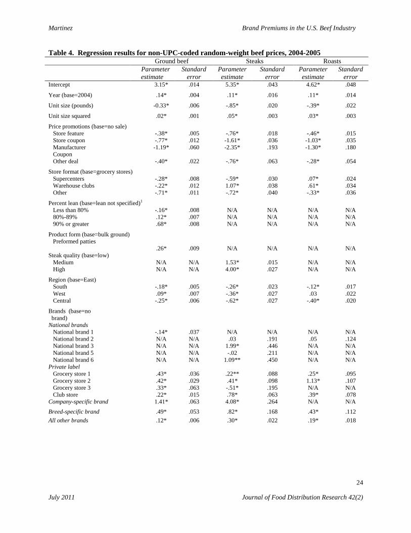
Martinez Brand Premiums in the U.S. Beef Industry
24
July 2011 Journal of Food Distribution Research 42(2)
Table 4. Regression results for non-UPC-coded random-weight beef prices, 2004-2005 Ground beef Steaks Roasts
Parameter
estimate
Standard
error
Parameter
estimate
Standard
error
Parameter
estimate
Standard
error Intercept 3.15* .014 5.35* .043 4.62* .048
Year (base=2004) .14* .004 .11* .016 .11* .014
Unit size (pounds) -0.33* .006 -.85* .020 -.39* .022
Unit size squared .02* .001 .05* .003 .03* .003
Price promotions (base=no sale)
Store feature -.38* .005 -.76* .018 -.46* .015
Store coupon -.77* .012 -1.61* .036 -1.03* .035
Manufacturer
Coupon
-1.19* .060 -2.35* .193 -1.30* .180
Other deal -.40* .022 -.76* .063 -.28* .054
Store format (base=grocery stores)
Supercenters -.28* .008 -.59* .030 .07* .024
Warehouse clubs -.22* .012 1.07* .038 .61* .034
Other -.71* .011 -.72* .040 -.33* .036
Percent lean (base=lean not specified)1
Less than 80% -.16* .008 N/A N/A N/A N/A
80%-89% .12* .007 N/A N/A N/A N/A
90% or greater .68* .008 N/A N/A N/A N/A
Product form (base=bulk ground)
Preformed patties
.26*
.009
N/A
N/A
N/A
N/A
Steak quality (base=low)
Medium N/A N/A 1.53* .015 N/A N/A
High N/A N/A 4.00* .027 N/A N/A
Region (base=East)
South -.18* .005 -.26* .023 -.12* .017
West .09* .007 -.36* .027 .03 .022
Central -.25* .006 -.62* .027 -.40* .020
Brands (base=no
brand)
National brands
National brand 1 -.14* .037 N/A N/A N/A N/A
National brand 2 N/A N/A .03 .191 .05 .124
National brand 3 N/A N/A 1.99* .446 N/A N/A
National brand 5 N/A N/A -.02 .211 N/A N/A
National brand 6 N/A N/A 1.09** .450 N/A N/A
Private label
Grocery store 1 .43* .036 .22** .088 .25* .095
Grocery store 2 .42* .029 .41* .098 1.13* .107
Grocery store 3 .33* .063 -.51* .195 N/A N/A
Club store .22* .015 .78* .063 .39* .078
Company-specific brand 1.41* .063 4.08* .264 N/A N/A
Breed-specific brand .49* .053 .82* .168 .43* .112
All other brands .12* .006 .30* .022 .19* .018

Martinez Brand Premiums in the U.S. Beef Industry
25
July 2011 Journal of Food Distribution Research 42(2)
Table 4. (Continued)
Regression results for non-UPC-coded random-weight beef prices, 2004-2005
Ground beef Steaks Roasts
Parameter
estimate
Standard
error
Parameter
estimate
Standard
error
Parameter
estimate
Standard
error Month (base=Dec.)
Jan. -.07* .010 -.21* .042 -.54* .036
Feb. -.08* .011 -.18* .043 -.64* .037
March -.09* .011 -.17* .043 -.59* .038
April -.08* .011 .06 .044 -.65* .038
May -.08* .010 .14* .043 -.69* .038
June -.07* .011 .13* .043 -.70* .038
July -.05* .011 .01 .043 -.67* .038
August -.02** .011 -.10** .042 -.71* .037
Sept. -.02 .011 -.05 .043 -.69* .038
Oct. -.04* .011 -.17* .042 -.67* .036
Nov. -.03* .011 -.12* .045 -.37* .041
No. of observations 115,287 87,717 37,851
Root MSE .69 2.40 1.31
Adjusted R2 .40 .31 .13
Highest condition
index2
17.07 15.81 16.68
White‟s Test3 3899.0 7301.0 1499.0
N/A=Not applicable.
Notes: One asterisk indicates the coefficient is statistically significant at the 1% level. Two asterisks indicates significance at the
5% level. 1Ground beef only. 2Low condition indices for each regression suggest that collinearity is not strong.
3White‟s test for heteroskedasticity was significant for each regression. Standard errors are from White‟s asymptotic consistent
covariance matrix, which provides heteroskedasticity-consistent test results for parameter estimates.
Source: Underlying data from Nielsen Homescan data.
Table 5. Summary statistics (continuous variables) and frequency distribution (discrete variables)
for UPC-coded ground beef Summary statistics for continuous variables
Variables Description Mean Std. Dev.
Dependent variable
P Price ($/lb) 2.25 0.84
Independent variables
SIZE Unit weight of the meat (pounds) 2.99 2.02
SIZESQ SIZE squared 13.01 17.08
Frequency distribution for independent discrete variables
Variables Description Percent of total
YEAR = 1 in 2005, 0 otherwise 52.5
Promotioni Type of promotion (base=no deal) 47.5
i= store feature 78.4
store coupon 19.4
manufacturer coupon 1.2
other deal 0.3

Martinez Brand Premiums in the U.S. Beef Industry
26
July 2011 Journal of Food Distribution Research 42(2)
Table 5. (Continued)
Summary statistics (continuous variables) and frequency distribution (discrete variables) for
UPC-coded ground beef
Variables Description Percent of total
StoreTypei Type of retailer (base=grocery stores) 65.1
i= supercenter 22.6
warehouse club 9.5
other 2.8
Region Region of household (base=East) 12.4
i= South 45.4
West 23.4
Central 18.7
Percent Leani Percent lean (base=lean not specified) 50.1
i= less than 80% 14.6
80%-89% 18.6
90% or greater 16.6
Product Typei Product type (base=bulk) 59.2
i=ground chub 4.8
preformed patties 35.9
Brandi Brands (base=no brand) 32.0
Top 20 brands
i=Brand 1 2.7
Brand 2 2.0
Brand 3 3.2
Brand 4 2.7
Brand 5 1.7
Brand 6 0.3
Brand 7 (company-specific brand) 2.2
Brand 8 4.5
Brand 9 0.6
Brand 10 2.3
Brand 11 0.4
Brand 12 2.4
Brand 13 0.3
Brand 14 0.3
Brand 15 0.3
Brand 16 0.5
Brand 17 0.6
Brand 18 0.4
Brand 19 0.4
Brand 20 0.4
Private label brands 35.2
All other brands 4.8
Monthi Month (base=Dec.) 6.2
i= Jan. 8.7
Feb. 6.6
March 7.1
April 8.1
May 10.4
June 9.8
July 11.0
August 9.4
Sept. 8.4
Oct. 7.9
Nov. 6.5
Number of observations 19,381

27
Effects of Elicitation Method on Willingness-to-Pay: Evidence from the Field Jared G. Carlberg and Eve J. Froehlich This paper compares willingness-to-pay (WTP) estimates elicited using three separate methods: in-store experi-mental auctions, a mailed survey with a cheap talk script included, and the same survey with no script. The products in question were four steaks bearing hypothetical brands representing various brandable attributes. It is found that WTP elicited using experimental auctions was the lowest, followed by WTP elicited by the mail survey with a cheap talk script, then the mail survey with no cheap talk script. Tobit and double-hurdle econometric models are used to identify factors influencing respondents’ WTP; model results are largely consistent with previous findings. A considerable number of empirical studies have been undertaken to determine willingness-to-pay (WTP) for a variety of products. Methods for eliciting WTP have evolved considerably since the earliest work in the field, resulting in a rich variety of experimental auction and contingent valuation methods now being available to re-searchers. Differences in cost and complexity among elicitation methods are considerable, and as a result, a wide variety of methods are com-monly used in both the field of experimental economics and for practical purposes in market research.
The body of literature exploring the effects of elicitation method upon WTP is vast. Extensive work has been undertaken to develop techniques to ensure precise estimates of WTP. However, some issues relating to effects of elicitation method upon WTP estimates remain unexplored; for example opportunities remain to compare results from field experiments with those from a mail survey using a common product. Addition-ally, the literature comparing econometric esti-mates based on data from different elicitation methods is relatively sparse.
There are three principal objectives of the re-search reported in this paper. The first is to de-termine the effect of elicitation method upon stated WTP for brand-name steaks in Canada. Carlberg is Associate Professor in the department of Agri-business & Agricultural Economics at the University of Manitoba. Froehlich is a Policy Analyst for the Canadian Grain Commission.
The authors gratefully acknowledge support from the National Beef Industry Development Fund of the Canadian Cattlemen's Association, along with the helpful comments of three reviewers and the Journal editor.
No researchers have previously attempted to compare WTP estimates from experimental auc-tions with those from mail surveys. The second objective is to quantify the effects of “cheap talk” (i.e. instructions regarding the presence and reasons for overstatement of bids in a hypo-thetical buying situation) in reducing hypothet-ical bias. If the form of experimental auction chosen is incentive compatible, then a compari-son of bids from these auctions with results from a survey incorporating cheap talk should illus-trate the extent to which cheap talk mitigates hypothetical bias. The third and final objective is to model the factors affecting WTP for the fic-tional steak brands developed for the research. The finding that econometric models based upon experimental auction vs. survey results have substantially different results has important im-plications from a research perspective.
Five sections comprise the remainder of this paper. First, the fictional steak brands developed for this research are described. An overview of the survey and experimental auction methodolo-gies is then provided, followed by a section out-lining the theory behind and econometric proce-dure used to estimate the WTP models. Results of the experimental auctions and surveys are then presented and discussed, along with esti-mates from the econometric models. The con-cluding section summarizes findings, acknowl-edges limitations, and makes suggestions for future work.
Steak Brands
Froehlich, Carlberg and Ward (2009) observe there are almost no fresh brand-name beef offer-ings in Canada, a marked difference from the

Carlberg and Froehlich Effects of Elicitation Method on Willingness-to-Pay: Evidence from the Field
28 July 2011 Journal of Food Distribution Research 42(2)
U.S. case. Accordingly, it was necessary to de-velop fictional brands to assess WTP. Four steak brands were developed for this research: a lo-cal/Canadian brand, a guaranteed tender brand, a natural beef brand, and an Angus brand. Froeh-lich, Carlberg and Ward (2009) provide further details on the process used to develop the brands and provide complete descriptions for each. Logos for the brands are given in Figure 1. WTP for Canada AAA beef, the second-highest grade of beef available (only 2% of beef grades above AAA) was also elicited from auction partici-pants and survey respondents.
Figure 1. Steak Brand Logos
Prairie Prime was the fictional local Canadi-an brand developed for the research. Steaks bearing this brand were described as being born and raised in the Canadian Prairies and were certified to grade AAA (equivalent to USDA choice) or higher. Additionally, Prairie Prime beef was guaranteed to be aged a minimum of 14 days. The guaranteed tender brand used to measure consumer WTP was called Tender Grill. Participants were informed this brand of beef was tested for tenderness using the Warner-Bratzler shear force test, which allowed the steaks to be certified as tender. The steaks were also described as having been aged a minimum of 21 days, but no grade guarantee was given.
The beef brand marketed as being derived from cattle never given growth hormones or an-tibiotics was called Nature’s Diamond. This “natural” beef brand also claimed animals were pasture-fed for 15 months prior to 120 days of grain finishing, were raised using environmen-tally friendly production methods, and received only chemical-free, natural feed and clean water. No guaranteed minimums for grade or dry aging time were provided. Original Angus was the fic-tional brand used in this research to represent the breed-specific characteristic that has enjoyed widespread demand for many years in the U.S. Steaks bearing this brand were positioned as being derived from beef that was grain fed, dry aged a minimum of 14 days, and verifiably An-gus in origin. Emphasis was placed upon careful selection of animals for inclusion in the branding program as well as upon involvement of both the national Angus breed association and independ-ent federal inspectors in monitoring and inspec-tion along the supply chain. Experiment and Survey Methodology
The use of experimental auctions to elicit WTP has risen as the selection of contemporary auc-tion mechanisms has grown. An experimental auction can be used to elicit a participant’s WTP in a manner that is designed to reflect their true valuation of a product. In an experimental auc-tion, measurement of WTP involves the use of actual money; this distinguishes the method from the hypothetical situation that exists when a survey method is used (Lusk et al 2001).
(a) Prairie Prime logo
(b) Tender Grill logo
(c) Nature’s Diamond logo
(d) Original Angus logo

Carlberg and Froehlich Effects of Elicitation Method on Willingness-to-Pay: Evidence from the Field
29 July 2011 Journal of Food Distribution Research 42(2)
An experimental auction is incentive compat-ible if it elicits values that reflect participants’ true WTP. There are numerous different experi-mental auction designs available to researchers, and incentive compatibility is often of para-mount importance in choice of design. For this condition to be met, the participant must have an incentive not to over or understate their bid: if a participant understates their bid, they risk not purchasing a product that is valuable to them, whereas overstatement may result in a situation where the respondent is forced to purchase a product for more than it is worth to them (Feld-kamp, Schroeder and Lusk 2005; Umberger and Feuz 2004).
Various types of experimental auctions can be used by researchers to elicit WTP. One of the most popular in recent years has been the Beck-er-DeGroot-Marshack (BDM) (1964) method. A number of agricultural economists have used this technique; examples include Feldkamp, Schroeder and Lusk (2005); Lusk et al (2001); and Lusk and Fox (2003). In a BDM auction, participants do not bid against one another; ra-ther they evaluate a particular good then are asked to submit a bid. If their bid is greater than a randomly selected price, the participant is obliged to pay the randomly selected price (i.e. not the amount they bid) for the item. BDM auc-tions are incentive compatible.
The BDM method was chosen for this re-search for a number of reasons. First, the ap-proach is easy to explain to participants and it is easy for them to understand relative to other auction designs (Lusk et al 2001). The BDM auction does not take repeated practice rounds for participants to learn how the auction works. Second, BDM auctions tend to have fewer non-responses and thus less non-response bias than other auction mechanisms and certainly less than contingent valuation (Lusk et al 2001). The BDM design has fewer non-responses because of ease of participation. Participants do not have to go out of their way on second day and drive to a location where another type of experimental auction would be conducted in a group setting (Feldkamp, Schroeder and Lusk 2005). In other words, there is less opportunity cost for the par-ticipants to partake in the study than in other experimental auction procedures. Response rates
are also generally higher than when contingent valuation is used and a mail survey is simply sent out.
The major alternative to experimental auc-tions is contingent valuation, a popular method used to elicit willingness-to-pay values from consumers. In agribusiness applications, typical-ly a novel product is described in detail and the participant is asked to state hypothetically in monetary terms how much they would be will-ing to pay for the good in question or are asked whether they are willing-to-pay a stated amount for the good. When consumers make decisions about what goods to purchase, they evaluate the utility of the attributes of each of the goods and maximize their expected utility by choosing a good with the optimal combination of attributes (Ness and Gerhardy 1994). Sometimes the con-sumer must make trade offs to achieve the most important attributes they desire in a good. For example, if a consumer’s primary concern is a ‘natural’ beef product, the consumer must be willing to trade off a low price attribute to obtain the ‘natural’ beef product. Contingent valuation is used to determine a consumer’s most pre-ferred attributes and ultimately most preferred goods. This type of method has been used by agricultural economists such as Neill et al (1994), Brown et al (1996) and Loomis, Gonza-lez-Caban and Gregory (1996), among others.
The use of a “cheap talk” script involves in-structing participants to respond as if they were making a real-world rather than hypothetical purchasing decision. Much of the early work behind cheap talk originated with Loomis, Gon-zalez-Caban and Gregory (1996), though they neither coined the term nor actually developed cheap talk itself. Using an open-ended survey instrument, they requested the subjects refrain from bidding what they thought to be the fair market value of the good and instead bid as though they were in a real market and actually had the opportunity to buy the good. Additional-ly, participants were asked to take their budget constraints into consideration when formulating their bid. Despite these efforts, the authors were unable to demonstrate that that these reminders were effective in eliminating hypothetical bias. Later work by Cummings and Taylor (1999) introduced cheap talk the way most researchers

Carlberg and Froehlich Effects of Elicitation Method on Willingness-to-Pay: Evidence from the Field
30 July 2011 Journal of Food Distribution Research 42(2)
use it today, and List (2001, 2003) extended the applicability of Cummings and Taylor’s cheap talk method to a real functioning market as op-posed to a classroom setting.
Data for this study were obtained using 274 BDM experimental auctions carried out in seven grocery stores from two major chains in and around the city of Winnipeg, Manitoba. Auc-tions were conducted at various times of the day during normal store hours on both weekdays and weekends and about 75% of the persons invited to participate agreed to do so. Each auction, conducted near the meat counter in participating grocery stores, took between five and seven minutes to complete after participants had read a two-page information sheet detailing the steak brands and their attributes. Additional infor-mation on the auction methodology and infor-mation provided to auction participants can be found in Froehlich, Carlberg and Ward (2009).
A mailed survey of 5,100 recipients was also conducted on a random sample of Canadian con-sumers excluding Quebec (due to its large fran-cophone population) and the three Canadian ter-ritories (mostly only frozen beef is available in the northern territories). The survey was de-signed to be as similar to the BDM auction as possible. Random addresses were purchased from a reputable market research firm. A Cana-dian one-dollar coin was included with the cover letter of each survey to provide an incentive to complete and return the questionnaire. A re-minder postcard was mailed to recipients three weeks following the original survey mailing.
Survey recipients also received a “Steak Fact Sheet” which described the hypothetical brands; this was the same information that was provided to experimental auction participants. Recipients were requested to complete a two page ques-tionnaire and mail it back in the prepaid postage envelope provided. Two separate treatments of the survey were used: the first contained, in ad-dition to the survey package (cover letter, busi-ness reply envelope, steak fact sheet and survey instrument), an information sheet discussing how people tend to overstate their willingness-to-pay for products and services in a hypothet-ical setting (this is referred to as the “cheap talk script”). This cheap talk script was identical to the one used in Lusk (2003) who made small
modifications to the original devised by Cum-mings and Taylor (1999). The script provides an overview of the problem of hypothetical bias, discusses why it may occur and requests that the respondent avoid hypothetical bias when com-pleting the survey. The other survey treatment simply received no cheap talk script.
Theory and Econometric Procedure
Lancaster (1966) observed that a major weak-ness of consumer demand theory at the time was that it omitted consideration of a good’s intrinsic properties. He noted that it is a good’s character-istics, rather than the good itself, that determine its value. This concept was extended by Ladd and Martin (1976), who modeled demand for a good as a function of a product’s characteristics, along with prices and income. A substantial number of subsequent empirical price analyses have employed this type of framework.
Hedonic price functions are commonly used to empirically estimate the relationship between a good’s price and its attributes. Goodman (1998) observes that although earliest use of this type of function is often attributed to Griliches (1958), in fact Court’s (1939) work on automo-bile price indices was the first use of such func-tions. A simple yet accurate description of he-donic price functions is provided by Nesheim (2006), who observes they “…describe the equi-librium relationship between the economically relevant characteristics of a product or service (or bundle of products) and its price.” This defi-nition seems in line with the Lancastrian frame-work outlined above, and so a hedonic function is employed in this paper to model WTP. He-donic models are sometimes criticized for a va-riety of reasons, including the so-called “adding up” problem whereby the value of all attributes, when summed, does not equal a product’s price. The reader is thus urged to interpret results with caution.
The model used to describe the relationship between stated WTP and the attributes of the branded steak in question as well as the demo-graphic characteristics of participants is

Carlberg and Froehlich Effects of Elicitation Method on Willingness-to-Pay: Evidence from the Field
31 July 2011 Journal of Food Distribution Research 42(2)
(1) WTPij = α + β1 × beef eaten + β2 × like name + β3 × confidence + β4 × gender + β5 × age + β6 × income + β7 × education + e,
where WTPij gives the willingness-to-pay for the jth steak stated by the ith respondent, beef eaten is the number of times per week the respondent eats beef, like brand is the respondent’s rating of how much they like the fictional brand on a 7-point Likert scale, confidence is the respondent’s self-assessment of their ability to select beef on a 7-point Likert scale, the remainder of variables are demographic characteristics of respondents, and e is the error term. All of age, income and education were measured as categorical varia-bles.
Because auction participants and survey re-spondents were not allowed to state negative amounts for premiums, the WTP data are left-censored (censored from below) (Lusk and Sho-gren 2007). As such, any econometric procedure used to estimate equation (1) must take this characteristic of the data into account; failure to do so could result in biased estimates (Amemiya 1973). The tobit model (Tobin 1958) can be used when left-censored data are encountered. This method explains the relationship between a non-negative latent dependent variable and one or more independent variables, and unlike ordi-nary least squares, takes explicit account of the limited nature of the dependent variable, yield-ing unbiased parameter estimates.
Cragg’s (1971) double-hurdle model recog-nizes that left-censored and uncensored data could be affected in disparate ways by various factors included in a model. For example, a giv-en regressor could exert a positive (negative) influence upon a respondent’s stated WTP, but a negative (positive) influence upon the likelihood that a respondent reports a zero bid for the good in question (Lusk and Shogren 2007). In order to use the double-hurdle technique, three separate models must be used: tobit, binomial probit, and truncated tobit. The log-likelihood statistic is captured from each, then used to calculate the following likelihood ratio statistic:
(2) LR = -2[lnLFTobit- lnLFBinomial Probit- lnLFTruncated Regression].
This test statistic is then compared to a critical value from the chi-squared distribution, with the degrees of freedom equal to the number of inde-pendent variables in the model. If the null hy-pothesis that the tobit model is the correct speci-fication is rejected, then the double-hurdle mod-el should be used. The interested reader is invit-ed to consult Lusk and Shogren (2007) for addi-tional details on use of the double-hurdle model.
Results
Table 1 shows the mean WTP by elicitation method for each of the fictional steak brands along with Canada AAA beef. Stated WTP elic-ited via the “conventional” survey is highest for each fictional brand, WTP from the survey con-taining a cheap talk script is the second-highest, Table 1. Mean Consumer Willingness-to-pay in each treatment and t-test results Steak Experimental Cheap Talk Conventional Auction Survey Survey ($/steak) ($/steak) ($/steak) Canada AAA
1.116 1.425a 1.472a,d
Prairie Prime
1.205 1.406a 1.481a,d
Tender Grill 1.317 1.431c 1.567a,d
Nature’s Diamond
1.312 1.576a 1.767a,e
Original Angus
1.308 1.641a 1.810a,e
a indicates statistically different from the experimental auction at α = 0.05. b indicates statistically different from the experimental auction at α = 0.10 c indicates not statistically different from the experimental auction d indicates not statistically different from the cheap talk survey e indicates statistically different from the cheap talk survey at α = 0.10 and bids from the experimental auctions are the lowest. In general, WTP was highest for the Original Angus steak, followed by Nature’s Di-amond, Tender Grill and Prairie Prime. Generic Canada AAA beef generally had the lowest stat-ed WTP. Table 1 also provides results of t-tests for statistical equivalence of average WTP by elicitation method.
The effectiveness of the cheap talk script in mitigating hypothetical bias can be quantified

Carlberg and Froehlich Effects of Elicitation Method on Willingness-to-Pay: Evidence from the Field
32 July 2011 Journal of Food Distribution Research 42(2)
approximately by calculating the difference in stated WTP for the five steaks across the two survey treatments. It should be noted that alt-hough average WTP for the cheap talk survey was lower than for the conventional survey for every beef brand, the WTP were only statistical-ly different for two brands; this implies that cau-tion should be exercised in interpreting these results. In percentage terms, the cheap talk script appears to have lowered stated WTP by between 2.8% (for Canada AAA beef) and 12% (for Original Angus). In general, the reduction in bids was smallest for the steaks with the fewest premium quality attributes (Canada AAA and Prairie Prime) and highest for those with several (Original Angus and Nature’s Diamond). If WTP estimates elicited by the BDM auction are regarded as incentive compatible, then the dif-ference between auction and cheap talk survey results approximates the amount of hypothetical bias remaining despite the use of a cheap talk script, of course recognizing that there are other potential reasons for the differences in stated WTP. Results from the auctions are lower by amounts ranging from 8.3% (for Tender Grill) to 27.7% (for Canada AAA beef).
Willingness-to-pay estimates elicited via BDM auctions were thus 20% lower on average than those elicited by a mail survey incorporat-ing a cheap talk script. This is a potentially im-portant finding for those engaged in market re-search—given the ease and relatively low cost of reaching a wide range of respondents via mail survey, the benefits of using this method are clear. However, researchers should interpret re-sults of such surveys with caution, noting the results here imply a significant amount of hypo-thetical bias exists in this contingent valuation method, even when a cheap talk script is used.
Treatment costs invariably influence selec-tion of elicitation method. For this research, per-survey costs were calculated to be $3.72, includ-ing stationary, printing, postage, student assis-tance and the $1 monetary incentive provided. Costs for the BDM auction amounted to $16.39 per response, including steaks, stationary (for steak information sheets), student assistance, and miscellaneous related costs. Though this cost discrepancy seems considerable, it must be re-membered that the response rate for auctions is
effectively one hundred percent—almost no costs are incurred for people who choose not to participate. By contrast, survey costs (except business reply postage, if it is used) are incurred for each recipient, regardless of whether they complete and return the survey.
Given this research’s survey response rate of 28%, approximately 3.57 surveys were required to generate one usable response, yielding a cost per usable response of $13.29 (3.57 × $3.72). It should be noted that this response rate is unusu-ally high for a “cold” mail survey (i.e. one being administered by an institution with whom the recipient has no prior relationship and pertaining to an issue with which the recipient has no ex-pected prior specialized knowledge); a lower response rate would result in a higher cost per usable response—for example, a 20% response rate would result in a cost of $18.60 per re-sponse, even higher than the BDM auction cost of $16.39. Given the apparent bias associated with survey results compared to the incentive compatible BDM auctions, the benefits of em-ploying a “cheap” mail survey instead of exper-imental auctions to measure WTP are somewhat questionable. Having said that, the costs of con-ducting market research across a wider geo-graphic region will increase dramatically if ex-perimental auctions rather than mail surveys are chosen.
Results of the tobit and double-hurdle econ-ometric models of WTP for each elicitation method and fictional brand are shown in Table2. Fifteen models were estimated (four brands plus Canada AAA for each of three elicitation meth-ods). The tobit model was rejected in favor of the double-hurdle model in most (but not all) cases. Like name exerted a positive and statisti-cally significant influence upon WTP in nearly every model, demonstrating the importance of careful development of brand name and logo, as well as product information, when measuring WTP for a new product.
Though not statistically significant in all cas-es, most of the demographic variable coeffi-cients were of the expected sign. There was no strong expectation on the sign for gender (fe-male = 0; male = 1); Feuz et al. (2004) found males willing to pay more than females for steaks with various quality attributes whereas

Carlberg and Froehlich Effects of Elicitation Method on Willingness-to-Pay: Evidence from the Field
33 July 2011 Journal of Food Distribution Research 42(2)
Lusk, Feldkamp and Schroeder (2004) discov-ered a higher WTP for females. This variable was only statistically significant in three models; in each case, males were found to have the high-er WTP. An interesting observation from the cheap talk survey was that for females, the brand with the highest mean willingness-to-pay was Nature’s Diamond, whereas for males it was Original Angus.
Respondent age was statistically significant in four models and exerted a negative influence upon WTP in each of those cases, indicating that older respondents were less receptive to the at-tributes associated with the brand name steaks than younger ones. This is in line with the find-ings of Feuz et al (2004) and Lusk, Feldkamp and Schroeder (2004) who also discovered a negative relationship between respondent age and WTP. Several other researchers, including Lusk et al (2001), found this relationship to be indeterminate.
As predicted by economic theory, respondent income exerted a pervasively positive impact upon WTP, although the relationship was only statistically significant in five of the models. This reaffirms the findings of Lusk and Fox (2002). Results for education, the final demo-graphic variable, were mixed: a positive and sta-tistically significant result was discovered for two of the models; in two others the coefficient was negative and significant. Perhaps most in-terestingly, the coefficient was positive and sig-nificant in the experimental auction and conven-tional survey models for the Nature’s Diamond brand, but negative and significant in the cheap talk model. Other research has discovered simi-larly mixed results: Lusk, Feldkamp and Schroeder (2004) found the relationship between education and WTP to be inverse, whereas Lusk and Fox (2002) found it to be positive. Similar to the findings of the present research, Lusk et al (2001) discovered the variable to have opposite signs in different treatments.
Econometric results for beef eaten are among the most intriguing—the relationship between WTP and this variable is significant and positive in three cases and negative in two others. Each of the positive findings is for WTP measured using an experimental auction, whereas both the negative findings come from data gathered using
the conventional survey treatment. Given the BDM auction has been demonstrated to be in-centive compatible and that auction participants were actual grocery shoppers approaching the meat counter in a supermarket, it is probably logical to characterize the experimental auction results as more reliable. This may indicate that purchasing decisions made in an experimental auction vs. hypothetical environment have con-sequences that go beyond mere differences in WTP estimates; it may be the case that results from mailed surveys are highly questionable in terms of reliability for this type of good. Similar-ly, each of the three cases where a negative and significant relationship was discovered between WTP and confidence used experimental auction data in estimation, while the two instances where a positive relationship were found used survey data. Again, it may be appropriate to characterize the BDM auction results as superior to those from the mailed surveys.
The fact that coefficients for the same varia-bles within a common model can possess statis-tically significant coefficients opposite in sign depending upon WTP elicitation method is a potentially important finding for researchers. Auction participants were active shoppers ap-proaching the meat counter in a grocery store whereas survey recipients are most likely in their home completing the survey; thus the im-portance of market research using “active” vs. “passive” (or hypothetical) shoppers may be im-portant. Understanding of factors affecting con-sumers’ purchasing decisions should be of ex-treme importance to firms in a marketplace. De-cisions on market segmentation and advertising expenditures can depend critically on this under-standing. Results reported here suggest careful selection of marketing research tools is in or-der—quantitative analysis based upon biased data has the potential to lead to suboptimal deci-sion making by firms.
Conclusions
The three objectives of the paper were to deter-mine the effect of elicitation method upon WTP for brand name steaks in Canada, to quantify the effects of cheap talk in reducing hypothetical bias, and to model the factors affecting WTP for

Carlberg and Froehlich Effects of Elicitation Method on Willingness-to-Pay: Evidence from the Field
34 July 2011 Journal of Food Distribution Research 42(2)
four fictional brands representing various steak attributes. Data from experimental auctions as well as cheap talk and “conventional” treatments of a mail survey were used in a hedonic model of consumer WTP.
Results of the research suggest that for each of the four fictional brands (as well as the gener-ic Canada AAA steak), average stated WTP from the “conventional” mail survey treatment was the highest, followed by that from the cheap talk treatment. Average WTP from the incentive compatible BDM auctions was the lowest. Alt-hough a cheap talk script does result in lower stated WTP than the “conventional” treatment in a mail survey, stated WTP is still much higher than that elicited using incentive compatible BDM experimental auctions. This indicates that significant bias remains, even when a cheap talk script is used. It was also discovered that there exists a relatively small per-response cost differ-ence between the two methods if non-responses by survey recipients are taken into account.
Findings from tobit and double-hurdle econ-ometric modeling suggest consumer preference for brand name and logo results in higher WTP for steaks bearing brands that represent various desirable steak attributes. Demographic varia-bles were found in several cases to exert statisti-cally significant effects upon WTP that were mixed in some cases, but largely in agreement with both economic theory and the findings of previous researchers.
It was discovered that data gathered using different WTP elicitation methods can generate conflicting results within a common model. Re-spondents’ self-assessed confidence in selecting beef was found to exert a negative effect upon WTP using experimental auction data, but a pos-itive effect (though only for Canada AAA steak) using survey data. Similarly, the frequency with which respondents eat beef exerted a positive effect upon WTP using data from experimental auctions but negative effects when survey data were used. This is potentially important to not only experimenters, but also to firms hoping to use quantitative analysis of market research data for strategic purposes.
A number of opportunities exist to extend this work. Similar comparisons of WTP data from different elicitation methods should be
used to determine whether the findings of this research are robust across experimental meth-ods. This research used experiments in the field to measure WTP from auctions and compare it to results from a mail survey; perhaps experi-ments in a laboratory setting could be used to reaffirm these findings. Alternative products could also be used—it would be worthwhile to explore the extent to which various factors affect WTP for other types of goods, and whether there are similar effects of treatment upon stated WTP levels for alternate products. References Amemiya, T. 1973. “Regression analysis when the
dependent variable is truncated normal.” Econo-metrica 41(6): 997-1016.
Becker, G.M., M.H. DeGroot and J. Marschak. 1964. “Measuring utility by a single-response sequential method.” Behavioural Science 9(3): 226-32.
Brown, T.C., P.A. Champ, R.C. Bishop and D.W. McCollum. 1996. “Which response format reveals the truth about donations to a public good?” Land Economics 72(1): 152-66.
Court, A.T. 1939. “Hedonic price indexes with auto-motive examples.” The Dynamics of Auto De-mand. General Motors Corporation, pp. 98-119.
Cragg, J.G. 1971. “Some statistical models for lim-ited dependent variables with application to the demand for durable goods.” Econometrica 39(5): 829-44.
Cummings, R.G. and L.O. Taylor. 1999. “Unbiased value estimates for environmental goods: A cheap talk design for the contingent valuation method.” American Economic Review 89(3):649-65.
Feldkamp, T.J., T.C. Schroeder and J.L. Lusk. 2005. “Determining consumer valuation of differentiated beef steak quality attributes.” Journal of Muscle Foods 16(1): 1-15.
Feuz, D.M., W.J. Umberger, C.R. Calkins and B. Sitz. 2004. “U.S consumers’ willingness to pay for flavor and tenderness in steaks as determined with an experimental auction.” Journal of Agricultural and Resource Economics 29(3): 501-16.
Froehlich, E.J., J.G. Carlberg and C.E. Ward. 2009. “Willingness-to-pay for fresh brand name beef.” Canadian Journal of Agricultural Economics 57(1): 119-37.
Goodman, A.C. 1998. “Andrew court and the inven-tion of hedonic price analysis.” Journal of Urban Economics 44(2): 291-8.

Carlberg and Froehlich Effects of Elicitation Method on Willingness-to-Pay: Evidence from the Field
35 July 2011 Journal of Food Distribution Research 42(2)
Griliches, Z. 1958. “The demand for fertilizer: an econometric reinterpretation of a technical change.” Journal of Farm Economics 40(3): 591-606.
Lancaster, K.J. 1966. “A new approach to consumer theory.” Journal of Political Economy 74(2): 132-57.
Ladd, G.W. and M.B. Martin. 1976. “Prices and de-mands for input characteristics.” American Jour-nal of Agricultural Economics 58(1): 21-30.
List, J.A. 2001. “Do explicit warnings eliminate the hypothetical bias in elicitation
procedures? Evidence from field auctions for sportscards.” American Economic Review 91(5): 1498-1507.
List, J.A. 2003. “Using random nth price auctions to value non-market goods and services.” Journal of Regulatory Economics 23(2):193-205.
Loomis, J., T. Brown, B. Lucero and G. Peterson. 1997. “Evaluating the validity of the dichotomous choice question format in contingent valuation.” Environmental and Resource Econom-ics 10(2): 109-23.
Loomis, J.B., A. Gonzalez-Caban, and R. Gregory. 1996. A Contingent Valuation Study of the Value of Reducing Fire Hazards to Old-Growth Forests in the Pacific Northwest. U.S. Dept. of Agricul-ture, Forest Service, Pacific Southwest Research Station, Albany, CA.
Lusk, J.L., J. Fox, T. Schroeder, J. Mintert and M. Koohmaraie. 2001. “In-store valuation of steak tenderness.” American Journal of Agricultural Economics 83(3): 539-50.
Lusk, J.L. and J.A. Fox. 2002. “Consumer demand for mandatory labeling of beef from cattle admin-istered grown hormones or genetically modified corn.” Journal of Agricultural and Applied Eco-nomics 37(1): 27-38.
Lusk, J.L. and J.A. Fox. 2003. “Value elicitation in retail and laboratory environments.” Economics Letters 79(1): 27-34.
Lusk, J.L. “Effectiveness of Cheap Talk On Consum-er Willingness-To-Pay for Golden
Rice.” American Journal of Agricultural Econom-ics 85(November 2003):840-56.
Lusk, J.L., T. Feldkamp and T.C. Schroeder. 2004. “Experimental auction procedure: Impact on the valuation of quality differentiated goods.” Ameri-can Journal of Agricultural Economics 86(2): 389-405.
Lusk, J.L. and J.R. Shogren. 2007. Experimental Auctions: Methods and Applications in Economic and Marketing Research. Cambridge: Cambridge University Press.
Neill, H.R., R.G. Cummings, P.T. Ganderton, G.W. Harrison and T. McGuckin. 1994.
“Hypothetical surveys and real economic com-mitment.” Land Economics 70(1): 145-54.
Nesheim, L. 2006. “Hedonic price functions.” Centre for Microdata Methods and Practice working pa-per CWP18/06, The Institute for Fiscal Studies, Department of Economics, University College of London.
Ness, M.R. and H. Gerhardy. 1994. “Consumer pref-erences for quality and freshness
attributes of eggs.” British Food Journal 96(1): 26-34.
Tobin, J. 1958. “Estimation of relationships for lim-ited dependent variables.” Econometrica 26(1): 24-36.
Umberger, W.J. and D.M. Feuz. 2004. “The useful-ness of experimental auctions in determining con-sumers’ willingness-to-pay for quality differenti-ated products.” Review of Agricultural Economics 26(2): 170-85.
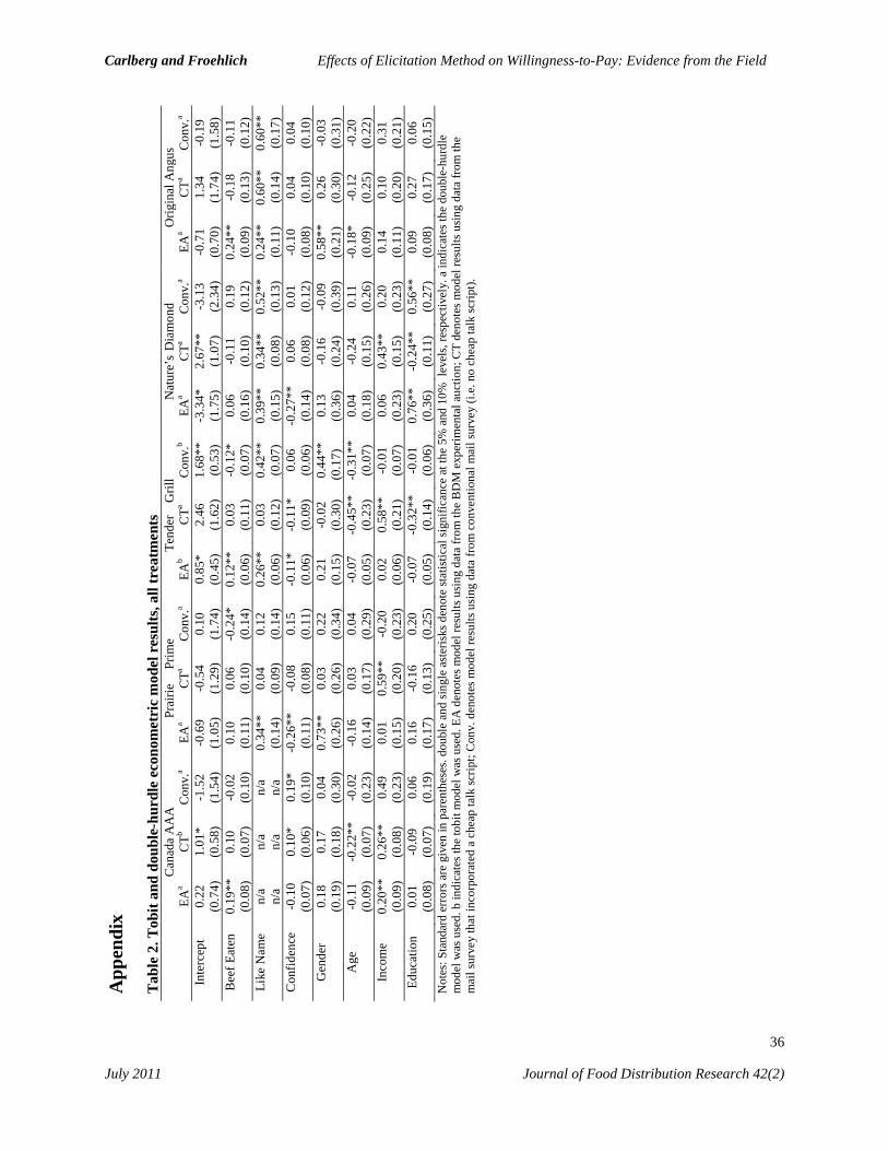
Carlberg and Froehlich Effects of Elicitation Method on Willingness-to-Pay: Evidence from the Field
36 July 2011 Journal of Food Distribution Research 42(2)
App
endi
x T
able
2. T
obit
and
doub
le-h
urdl
e ec
onom
etri
c m
odel
res
ults
, all
trea
tmen
ts
C
anad
a A
AA
Pr
airie
Pr
ime
Tend
er
Gril
l N
atur
e’s
Dia
mon
d O
rigin
al A
ngus
EAa
CTb
Con
v.a
EAa
CTa
Con
v.a
EAb
CTa
Con
v.b
EAa
CTa
Con
v.a
EAa
CTa
Con
v.a
Inte
rcep
t 0.
22
1.01
* -1
.52
-0.6
9 -0
.54
0.10
0.
85*
2.46
1.
68**
-3
.34*
2.
67**
-3
.13
-0.7
1 1.
34
-0.1
9
(0.7
4)
(0.5
8)
(1.5
4)
(1.0
5)
(1.2
9)
(1.7
4)
(0.4
5)
(1.6
2)
(0.5
3)
(1.7
5)
(1.0
7)
(2.3
4)
(0.7
0)
(1.7
4)
(1.5
8)
Bee
f Eat
en
0.19
**
0.10
-0
.02
0.10
0.
06
-0.2
4*
0.12
**
0.03
-0
.12*
0.
06
-0.1
1 0.
19
0.24
**
-0.1
8 -0
.11
(0
.08)
(0
.07)
(0
.10)
(0
.11)
(0
.10)
(0
.14)
(0
.06)
(0
.11)
(0
.07)
(0
.16)
(0
.10)
(0
.12)
(0
.09)
(0
.13)
(0
.12)
Li
ke N
ame
n/a
n/a
n/a
0.34
**
0.04
0.
12
0.26
**
0.03
0.
42**
0.
39**
0.
34**
0.
52**
0.
24**
0.
60**
0.
60**
n/a
n/a
n/a
(0.1
4)
(0.0
9)
(0.1
4)
(0.0
6)
(0.1
2)
(0.0
7)
(0.1
5)
(0.0
8)
(0.1
3)
(0.1
1)
(0.1
4)
(0.1
7)
Con
fiden
ce
-0.1
0 0.
10*
0.19
* -0
.26*
* -0
.08
0.15
-0.1
1*
-0
.11*
0.06
-0.2
7**
0.06
0.
01
-0
.10
0.04
0.04
(0
.07)
(0
.06)
(0
.10)
(0.1
1)
(0.0
8)
(0.1
1)
(0.0
6)
(0.0
9)
(0.0
6)
(0.1
4)
(0.0
8)
(0.1
2)
(0.0
8)
(0.1
0)
(0.1
0)
Gen
der
0.18
0.
17
0.04
0.
73**
0.
03
0.
22
0.
21
-0
.02
0.44
**
0.
13
-0
.16
-0.0
9
0.
58**
0.
26
-0
.03
(0
.19)
(0
.18)
(0
.30)
(0
.26)
(0
.26)
(0
.34)
(0.1
5)
(0
.30)
(0
.17)
(0.3
6)
(0
.24)
(0
.39)
(0.2
1)
(0.3
0)
(0.3
1)
Age
-0
.11
-0.2
2**
-0.0
2 -0
.16
0.03
0.
04
-0
.07
-
0.45
**
-0.3
1**
0.
04
-0
.24
0.11
-0.1
8*
-0.1
2
-0.2
0
(0.0
9)
(0.0
7)
(0.2
3)
(0
.14)
(0.1
7)
(0.2
9)
(0
.05)
(0.2
3)
(0
.07)
(0.1
8)
(0
.15)
(0
.26)
(0.0
9)
(0.2
5)
(0.2
2)
Inco
me
0.20
**
0.26
**
0.49
0.
01
0.
59**
-0
.20
0.02
0.58
**
-0.0
1
0.
06
0.
43**
0.20
0.
14
0.
10
0.31
(0.0
9)
(0.0
8)
(0.2
3)
(0.1
5)
(0.2
0)
(0
.23)
(0.0
6)
(0.2
1)
(0
.07)
(0.2
3)
(0.1
5)
(0
.23)
(0.1
1)
(0.2
0)
(0.2
1)
Educ
atio
n 0.
01
-0.0
9
0.
06
0.16
-0.1
6
0.
20
-0
.07
-0
.32*
* -0
.01
0.
76**
-0
.24*
* 0.
56**
0.09
0.27
0.06
(0.0
8)
(0.0
7)
(0.1
9)
(0.1
7)
(0.1
3)
(0
.25)
(0.0
5)
(0.1
4)
(0
.06)
(0
.36)
(0.1
1)
(0.2
7)
(0
.08)
(0
.17)
(0.1
5)
Not
es: S
tand
ard
erro
rs a
re g
iven
in p
aren
thes
es. d
oubl
e an
d sin
gle
aste
risks
den
ote
stat
istic
al si
gnifi
canc
e at
the
5% a
nd 1
0% l
evel
s, re
spec
tivel
y. a
indi
cate
s the
dou
ble-
hurd
le
mod
el w
as u
sed.
b in
dica
tes t
he to
bit m
odel
was
use
d. E
A d
enot
es m
odel
resu
lts u
sing
dat
a fro
m th
e B
DM
exp
erim
enta
l auc
tion;
CT
deno
tes m
odel
resu
lts u
sing
data
from
the
mai
l sur
vey
that
inco
rpor
ated
a c
heap
talk
scrip
t; C
onv.
den
otes
mod
el re
sults
usi
ng d
ata
from
con
vent
iona
l mai
l sur
vey
(i.e.
no
chea
p ta
lk sc
ript).

37
Political Economy of Medical Food Reimbursement in the U.S. Adesoji O. Adelaja, Amish Patel and Yohannes G. Hailu Medical foods, which fall in the gray area between food and drugs, are a necessity for persons with inborn errors of metabolism. Being more expensive than regular foods, some U.S. states have mandated insurance companies to pro-vide coverage for the afflicted community. To investigate the legislative adoption process, this paper develops a political economy model of medical food reimbursement and coverage policy. Analytical cross-state logit regression models confirm the positive influences of metabolic clinics and the political clout of the afflicted community on the probability of adoption. The countervailing interest of the insurance industry and the afflicted community were also confirmed. Results suggest that efforts by medical food companies to influence the political process could yield food market and distribution channel opportunities in states contemplating legislative adoption. Introduction A medical food is “a food which is formulated to be consumed or administered entirely under the supervision of a physician and which is intended for the specific dietary management of a disease or condition for which distinctive nutritional requirements, based on recognized scientific principles, are established by medical evalua-tion” (U.S. Congress, 1988). Like prescription drugs, the costs of which are typically covered by insurance companies (via state legislative mandates), medical foods are a necessity for a healthy and normal life for individuals with met-abolic disorders. However, medical foods are also close to regular foods, whose costs are typi-cally absorbed by consumers and are not cov-ered under drug insurance. Because medical foods are at the boundary between food and drugs, they are controversial and represent a gray area of food and health policy.
Drug reimbursement policy falls within the realm of powers granted to the states. States, however, differ in demographic and other char-acteristics, and therefore the propensity to adopt Adesoji O. Adelaja is the John A. Hannah Distinguished Professor in Land Policy in the Department of Agricultural, Food and Resource Economics (AFRE) at Michigan State University (MSU). Amish Patel is Vice President, DP Sys-tems Inc., Midlothian, Virginia. Yohannes G. Hailu is Vis-iting Assistant Professor at AFRE.
The authors appreciate the insights, ideas and other contributions of Brian Schilling, Louis Cooperhouse, Casey Roberts, other executives of the Menudirect Corporation and students in the special undergraduate research course on the issue of medical foods. This paper is dedicated to Therese and Kelly Waters of Okemos, Michigan.
insurance-mandated medical food reimburse-ment policy and the level of reimbursement cho-sen. Prescription drugs are subsidized or reim-bursed by healthcare plans from insurance com-panies based on the state’s reimbursement schedule. However, prescription or medical foods are not always covered, due in part to op-position by insurance companies1.
The afflicted and members of their family stand to gain by lobbying for adoption of medi-cal food reimbursement policy. Given the dis-parity in the costs of medical and non-medical foods, the health, purchasing power and quality of life of the afflicted community are impacted 1
By voluntarily extending coverage to medical foods, an insurance company can attract a disproportional number of the afflicted. Hence, the company may still not extend coverage unless forced by legislation even when the cost of mitigating the adverse effects of ingesting the wrong food exceeds the cost of providing coverage for medical foods. Products with-in the medical foods category include special formu-lations for patients with celiac sprue (CS), phenylke-tonuria (PKU), irritable bowel disease (IBD), Urea Cycle Disorder (UCD), Glycogen Storage Disorder (GSD), Propionic Acidemia (PA), Methyl Malonic Acidemia (MMA), maple syrup urine disease (MSUD), and diabetes. For patients with these disor-ders, medical foods are almost unavoidable as the afflicted must avoid specific foods, components or nutrients to prevent illness or death or must ingest increased amounts of certain metabolites to stimulate a specific metabolic pathway for survival (Bistrian, et al., 1976). Studies have shown that even small reduc-tions in intake can yield substantial health benefits. (Browner, et al., 1991; Zarkin and Anderson, 1992).

Adelaja et al. Political Economy of Medical Food Reimbursement in the U.S.
38 July 2011 Journal of Food Distribution Research 42(2)
by such adoption. The physicians and dieticians of the afflicted, the medical food industry, and facilities that provide metabolic treatment, also called metabolic clinics2, usually join the afflict-ed in advocating for legislative adoption of such policy. The medical foods industry could benefit from legislative adoption as such policy can lower the prices of their products and enhance consumer affordability and market penetration. The medical foods area is one where efforts by producers and distributors to organize the pro-ponents of adoption lobby law makers can create a game-changer in the development of new mar-ket opportunities in a state.
Insurance companies are known to almost consistently oppose such legislation based on the argument that it decreases profitability by in-creasing insurance payout per capita and the cost of insurance to the non-afflicted community. Perhaps, their real concern is that once a state adds some medical foods to the reimbursement schedule, it becomes easier to add other items that may not be real medical necessities. Con-sistent with their stand on healthcare in general, the non-afflicted community has been silent in the reimbursement debate. Perhaps, the small size of the afflicted community suggests mini-mal impacts on their budget, especially when many of them are covered by employer paid in-surance. Information on the determinants of leg-islative adoption, including the marginal impact of lobbying efforts on the probability of adop-tion, is therefore of significant value, not only to the afflicted community and other pro-reimbursement advocates, but also to the insur-ance companies and other opponents of reim-bursement. Medical food producers and distribu-tors are particularly interested, as legislative adoption can bring the entire community of af-flicted people into the market, due to the cost eliminating nature of adopted legislation. Such 2 A metabolic clinic is a facility focused on helping patients with metabolic disorders. It has a broad range of specialists ranging from nutritionists, nurses and social workers to metabolic geneticists, genetic counselors and psychologists. According to the Mayo Clinic, such clinic provides comprehensive diagnos-tic and management services for people with known or suspected inborn errors of metabolism (http://www.csmc.edu/2548.html).
information can be used in predicting the likeli-hood of policy change, medical food legislation in states that have not yet adopted, the potential benefits of lobbying efforts, as well as in choos-ing optimal strategy for impacting such change.
Regarding the political dynamics of legisla-tive and policy adoption, several studies suggest various legislative causal factors, including (1) the characteristics of the policy and its goals (Bardach, 1997; Derthick, 1972; Rosenbaum, 1976; Sabatier and Mazmanian, 1983); (2) the characteristics of implementing agencies (Ed-wards, 1980; Nakamura and Pinderhughes, 1980); and (3) the beliefs and attitudes of key policy actors (Bardach, 1997; Marshall et al., 1986; Mitchell, 1981; Sabatier and Mazmanian, 1983; Van Horn and Van Meter, 1976). Aaron (2002) identified the escalating costs of health care expenditures, access to healthcare, the qual-ity of healthcare and competition between healthcare insurance companies as important determinant factors in adopting health care poli-cies. In addition, Weekes (1997) identified con-sumer demand for alternative health care ser-vices and the growing interest of private insurers in providing coverage for various alternative treatments as another determinant in adopting health care policies.
While some literature exists on the usage and need for medical foods, despite the intense con-troversy surrounding the issue, to the best of our knowledge, nothing is available in the economic, political and marketing literature on the legisla-tive adoption process. Given the importance of such analysis, this study conceptualizes the de-terminants of legislative adoption of medical food reimbursement policy, including (1) politi-cal and economic powers and motives, (2) socio-economic, demographic, and other legislative adoption factors, and (3) interstate proximity to other adopters (spillover effects). An empirical logit model is estimated to evaluate the effects of key factors hypothesized to determine the passage of medical food laws mandating insur-ance industry reimbursement. Implications for the lobbying efforts of medical foods companies are also highlighted.

Adelaja et al. Political Economy of Medical Food Reimbursement in the U.S.
39 July 2011 Journal of Food Distribution Research 42(2)
Background Like prescription drugs, medical foods are nec-essary for healthy and normal life for individuals with metabolic disorders. According to FDA, for a product to be considered as Medical Food, it must be 1) food for oral or tube feeding 2) la-beled for a specific medical disorder, disease or condition and 3) intended to be used under med-ical supervision. Diabetes mellitus (DM), malab-sorption, phenylketonuria (PKU), homocystinu-ria and maple syrup urine diseases (MSUD) are examples of metabolic disorder diseases (Otles and Akcicek, 2002). An example of medical foods is gluten-free cereal to avoid wheat aller-gies, health bars with added medication, and transgenic plants for oral vaccination against infectious diseases, and transgenic cows and lactoferrin for immune enhancement.
The high procurement cost limits the ability of the afflicted to enjoy good health and quality of life. As shown in Table 1, using the example of PKU, medical foods solutions can be 131% to 3833% more expensive than its normal food counterpart.3 Clearly, for families with individ-uals whose survival depends on medical foods, staying healthy could be a financial challenge.
Source: National PKU News, Table of Data on Food Costs, http://www.pkunews.org/rights/lobby5.htm July, 2003.
3 By extrapolation, per capita annual cost of medical foods is about $14,000, compared to $3,800 for nor-mal food. By adding one afflicted member, the food bill for an average family of 3 with a 1999 mean fam-ily income of $62,636 (US Census Bureau, 1999) could rise from $11,400 (18%) to $21600 (36%).
In response to concerns about the burdens on individuals/families with metabolic disorders requiring medical food for survival, the U.S. Congress adopted the Orphan Drug Amend-ments (U.S. Congress, 1988) and the Nutritional Labeling and Educational Act (U.S. Congress, 1990). These legislations better defined the drug status of medical foods and provided the founda-tion for state mandates requiring the provision of insurance company reimbursement. Today, the adoption of medical foods reimbursement policy varies by state.4 When reimbursement legisla-tion exists in a state, typically, governing laws provide reimbursement schedules for medical formula and/or food which may set a limit on the annual dollar amount of reimbursement and/or on age.5
The chronology and features of state adop-tion of medical food reimbursement policy are depicted in Table A.1 in the Appendix. The cri-teria for medical foods reimbursement by state is presented in Table A.2. The timeline for federal policies on medical foods is further delineated in Table A.3. As of July 2003, consumers in 29 states could expect to receive reimbursement or coverage for medical food expenditures they incur through insurance companies, while con-sumers in 21 states could be expected not to.
4 For example, Kentucky limits reimbursement of medical foods to $4,000 annually with no age re-striction. Maryland sets no dollar or age restrictions. Colorado only covers males below the age of 22 and females below the age of 36 and imposes no annual dollar restriction. 5 A “reimbursement schedule” is a legislative man-date on a state agency or insurance industry.
Table 1. Cost Comparison of Low Protein Products and their Regular Counterparts Description
of Food Regular Food
Low Protein Food
Percentage Increase
Shipping & Handling
Spaghetti (16 oz) $1.25 $5.00 300%
Flour (1 pound) $0.18 $7.08 3833%
Crackers (16 oz) $0.79 $15.85 1906% $5 to $25
Cream Filled Wafers $0.49 $2.95 502% per order
Jello (3 oz.) $0.55 $1.27 131%
Tomato Sauce (4 oz.) $0.25 $4.07 1528%

Adelaja et al. Political Economy of Medical Food Reimbursement in the U.S.
40 July 2011 Journal of Food Distribution Research 42(2)
The checkered pattern of legislative adoption, coupled with the typical deliberate nature of such processes, suggests the need to explain the factors that lead to state of adoption of medical foods reimbursement policy. The fledgling med-ical foods industry, whose survival or emergence depend largely on state-level legislative adop-tion, is particularly interested in understanding this process as it could inform the efforts to allo-cate marketing funds toward organizing, advo-cacy and lobbying for legislative adoption. Conceptual Framework The political environment of states may play an important role in shaping public policies. States vary in terms of the adoption of health policies and particular health care programs (Miller, 2005). For example, in the case of medical foods, some states have adopted full or partial reimbursement and other states have not (Table A.1). What influences some states to likely sup-port medical food reimbursement legislation? Understanding the fundamental factors that in-fluence states’ adoption of specific policies or legislation is crucial for both the afflicted com-munity and insurance companies to influence the political process towards their respective ad-vantages.
Dye (1966) identified several additional po-litical, socio-economic and demographic factors that determine legislative adoption: interparty competition, division of party control, the elec-toral system and voter participation, and degree of inequality in voter representation6. Interparty competition refers to the initiation of new legis-lation as a means of competing for votes. Divi-sion of party control refers to the extent of con-trol of the state government by either party, Democrats or Republicans. Each party tends to favor certain types of legislation. For instance, usually Republicans support legislations that 6 The dominant party is expected to be more likely to get its policies passed. Lower income, lower status, poorly educated, and non-white groups, which typi-cally support democrats, are expected to have lower voter participation rates. Finally, less well represent-ed groups are less likely to have policies evolve that benefit them (Dye, 1966).
promote less regulation while Democrats sup-port more regulation and government interven-tion (Cook et al., 1988; Grogan, 1994). Consid-ering Medical Foods Reimbursement, Demo-crats may favor medical food reimbursement legislation while Republicans may oppose this legislation as they favor less regulation and gov-ernment intervention. Since people differ in their needs, the policy intervention they support dif-fers with their socio-economic characteristics such as income, age and race groups (Shingles, 1989; Brown, 1988; Coughlin, 1980). Dye (1966) suggests that adoption of legislations is influenced by policy preference of the constitu-encies, for example, urban versus rural constitu-encies or rich versus poor constituencies.
The political processes of neighboring states will tend to have an impact on the legislative process of nearby states. Rosenbaum (1976) highlights the influence of neighborhood politi-cal process and its spillover effect. Politicians tend to follow the political process of their neighboring states mainly because nearby states tends to face similar challenges, and to avoid movement of people from neighborhood states (Miller, 2005; Rosenbaum, 1976).
This paper, therefore, utilizes the political economy framework to identify the determinants of medical foods reimbursement policy adop-tion. The framework is based on Dye’s basic infrastructure (Dye 1975). We focus mainly on the choice by the government to pass legislation mandating the insurance industry to reimburse for medical foods.
The competing interest groups include the in-surance community and the afflicted communi-ty. The interest of the non-afflicted community is accounted for in the objective function of the insurance community. Hence, both the insurance industry (as an agent of the non-afflicted) and the afflicted community (supported by their sympathizers) exert pressure on the legislature to make choices based on their relative strength in the political arena and their economic interests.
The insurance industry’s actions are based on the desire to maximize the utility it derives from collecting insurance premiums, turning a profit, and generating any beneficial externalities. It tries to keep premiums down to optimize the utility of its clientele and its own long-term sur-

Adelaja et al. Political Economy of Medical Food Reimbursement in the U.S.
41 July 2011 Journal of Food Distribution Research 42(2)
vival (such as increased public health and in-creased patronage). Therefore, it is expected that the larger the size of the insurance community (companies, clients and employees), the more influential the opponents of legislative adoption, and the less support for legislation. On the other hand, afflicted households wish to maximize utility (or quality of life) from insurance cover-age of traditional healthcare costs plus medical foods.7 Hence, the afflicted population is hy-pothesized to have a negative impact on the profit objective of the insurance industry by in-creasing healthcare payouts per capita.
The legislature (the ultimate decision maker) must then balance the interests of these interest groups in maximizing its own objectives, subject to pressures from the electorate and from com-peting economic and political interest groups (Tullock, 1967; Stigler, 1971; Peltzman, 1976). It, therefore, advances legislation that maximizes public acceptance. Insurance Companies
The representative insurance company earns income, yi, from providing health insurance cov-erage to the community of covered people (q): such that yi = pq – c(q) - αβ(x), where p is the average premium collected for health insurance coverage, c is the marginal cost of providing health insurance coverage, x is the number of individuals with the need for medical foods or the afflicted community size, β is expected cost per unit to provide medical food reimbursement for the afflicted community, β(x) is the total ex-pected cost of providing medical foods reim-bursement for the afflicted community (where βx,, βxx > 0) and α is a measure of the proportion of the total or maximum medical foods reim-bursement cost that insurance companies are expected to bear. Increased premiums or reduced healthcare coverage are irksome to both the af-flicted and non-afflicted communities. αβ(x) is the externality by the afflicted community that
7 Non-afflicted household also try to maximize their utility, except that the need for medical food cover-age is not a big issue for those who prefer not to bear the cost of the afflicted community.
can be either absorbed by the insurance compa-ny (with an impact on premiums) or by the af-flicted community. q – x is the number of people in the non-afflicted community. The extent of externalities associated with medical foods is assumed to be an increasing function of the community of covered people since the larger the population, the larger the afflicted communi-ty ( i.e. xq , xqq >0)8.
The insurance industry attempts to prevent the afflicted community from transferring their externality to them by lobbying the government not to legislate regulations that would force re-imbursement and thereby result in premium in-creases. Alternatively, the afflicted community would seek to have government force on the in-surance industry such measures that reduce the burden on them and spread the cost of medical food to others. Whether or not the externality is transferred or not is given by α. When α is low enough, one might observe the absence of medi-cal food reimbursement law. High values of α might imply the presence of medical food reim-bursement law. In the extreme scenario of α = 0, the afflicted community assumes responsibil-ity for full medical food cost while α = 1 may imply that insurance companies are responsible for the full reimbursement of medical food cost. Afflicted households are likely to lobby for α=1 or full coverage and insurance companies for α=0 or avoid complete reimbursement. The government must carefully weigh the sentiments of the two communities and the possible elec-toral impacts of their decision in choosingα.
The utility function of the insurance compa-ny may be expressed as:
(1) ui(g) = ui(yi, x, h) = ui[pq – c(q) -
αβ(x(q)), x, h],
where h is the health index or a measure of the general level of health in the community. Healthy people reduce health insurance payouts. While general health is important, and insurance companies generate a lot of it, its impact on 8 We assume that the non-afflicted community and insurance companies are not in conflict regarding the desire to keep premiums down.

Adelaja et al. Political Economy of Medical Food Reimbursement in the U.S.
42 July 2011 Journal of Food Distribution Research 42(2)
medical foods is likely to be miniscule. There-fore, we assume the marginal utility of the gen-eral level of health is very low to insurance companies. Thus, for simplicity, it is ignored in the insurance companies’ utility function. The utility function obeys the restrictions ui
y > 0, and ui
x, uixx, ui
yy, uixy < 0 where the superscript i de-
notes the insurance companies. The convexity of the cost function implies cq, cqq > 0. The insur-ance company chooses the scale of health insur-ance coverage to the public to maximize utility as defined by (1). The first order condition for an interior maximum is:
(2) p = cq + αβxxq – xq(uix / ui
y). As shown in equation (2), the scale of insur-
ance enrollment is chosen optimally so as to equate the price charged for healthcare coverage (through premiums) to the sum of (1) the mar-ginal cost of providing standard health insurance coverage to the public (2) the marginal cost of covering medical food purchased by the afflicted community, and (3) the money value of the disu-tility of incremental externalities. Solving this equation, we can express the optimum enroll-ment by the insurance company as a function of α(q* = q*(α)). That is:……………………….
(3) ,0))(()()(
)(2
*
<+++−+++
+−= i
xqqxxqqqxqqiy
ixxq
ixyq
ixyq
iyy
ixyq
iyyqx
iy
uxxxcuuxuxuxuuxuxu
ddq
βααβθθθθββ
α
where θ = p - cq - αβxxq > 0. From equation (3), the insurance company’s optimum coverage is a monotonically decreasing function of α.
To establish the curvature of the q*(α) function, further assumptions are necessary. If utility function is linear and c, x and β functions are quadratic, then equation (3) reduces to:
(4) ixqqxxqqqxqq
iy
qxiy
uxxxcuxu
ddq
+++=
))(( 2
*
βααββ
α;
and
(5) 22
2*
2*
22
2
*2
)))(((
))(3()())(()()((ixqqxxqqqxqq
iy
xxqqxxxqqqqxiyxxqqqxqq
iyxxq
iyqqx
iy
uxxxcu
xxddqxxxu
ddqxxcuxuxu
dqd
+++−
+++++−+=
βααβ
ββα
βαβα
βααβββ
α
A sufficient condition for d2q*/dα to be positive is that βxxqq + (xq)2βxx > -3αxqxqqβxxdq*/dα. This is auto-matically satisfied if either x or β is linear in its argument. If both of them are linear, then d2q*/dα2 = 0, implying that q*(α) is a linear function. For the rest of the analysis we assume that d2q*/dα2 ≥ 0.
Afflicted Community
The utility function of the afflicted community is given by: ud(yd, x, h). Afflicted households fa-vor healthcare coverage for medical food, and unlike insurance companies, value such increas-es in healthcare coverage at the margin. Such health index comprises of the private industry healthcare coverage λ and government provision of coverage ω. Therefore h = λ + ω. Since the health index is monotonically related to provid-ing health insurance coverage to the public, it is possible to write λ as an inverse function of
insurance company enrollment. That is, λ = λ(q), and λq > 0 such that hq > 0.
The afflicted community chooses the level of q by choosing x such that ud
xxq + udhhq = 0. That
is, the disutility associated with covering the afflicted community is set equal to the utility derived from the positive externality of the health index. This equation may be solved to express afflicted community desired enrollment q as a function of afflicted community income and government expenditure on health issues. That is:
qd = qd(yd, ω). It can be shown that:

Adelaja et al. Political Economy of Medical Food Reimbursement in the U.S.
43 July 2011 Journal of Food Distribution Research 42(2)
(6) )()( 2 d
hhqdxhqq
dxhqqq
dxxqq
dy
qdhyq
dxy
d
d
uhuxuxhxuxuhuxu
dydq
++++
+=
λ; and
(7) )()( 2 d
hhqdxhqq
dxhqqq
dxxqq
dy
qdhhq
dxh
d
uhuxuxhxuxuhuxu
ddq
++++
+=
λω That is, an increase in the afflicted community income should raise the demand for health cov-erage but lower the demand for insurance com-panies’ coverage of medical food expenditures, ud
hy < 0. The marginal utility associated with coverage also declines if coverage implies much higher premiums, uxh < 0. The law of diminish-ing marginal utility ensures that ud
hh < 0. It is seen that under these conditions dqd/dyd and dqd/dω are both unambiguously negative. Government
The government comprises elected representa-tives of the afflicted community and insurance industry. It behaves rationally in the sense that it only decides on such measures (or legislation) as it believes would raise its electoral prospects. Recall that the non-afflicted community is very silent in the reimbursement debate on medical foods. However, insurance industry employees are not and such companies, though their finan-cial support for candidates, can mobilize votes of the non-afflicted. The government’s utility function may thus be regarded the same as the expected total vote function.
The utility function of the government is ex-pressed as: where I = a proxy for voting influence of insur-ance companies on the non-afflicted community (including its employees), A = voting population of the afflicted community, Πj = probability that the average jth group will vote for the govern-ment, j = i, d; γ = an index of the political clout of the insurance companies and the non-afflicted community, υ = an index of the political clout of the afflicted community, and θ, Ω = other exog-enous variable that may influence Πj.
Since an increase in α raises the cost of cov-erage and reduces insurance companies income or ability to cover, insurance companies are like-ly to reduce political support for a government that imposes a higher α on them, such that Πi
α < 0. On the other hand, an increase in α reduces the burden on the afflicted and raises the proba-bility that the afflicted community would vote for the government; Πd
x < 0. At any given level of α, x and q, an increase in the income of the afflicted households makes them desirous of an increase in α such that they are less likely to politically support the government unless it takes measures to raise α, implying Πi
xy < 0. For a similar reason, Πd
xω, Πiαγ, < 0. It is further as-
sumed that Πiαα and Πd
xx, are also negative. The government chooses α in order to max-
imize electoral support. The first order condition for maximization is:
This equation defines a maximum, provided d2V/dα2 < 0. Hence,
(10)
Given the earlier assumptions, this expression is negative such that the equation above unambig-uously defines a maximum. The equation simply states that in order to maximize V, the govern-ment sets the value of α such that the expected marginal decrease in insurance companies’ and non-afflicted community votes due to an in-crease in x is just offset by the expected margin-al increase in afflicted community’s votes. Solv-ing the equation, we can find optimum α* as a function of the exogenous variables: α* = α*(I, A, γ, θ, yd, ω, υ; Ω).
(8) uG = V =IΠi(α, γ; θ) + AΠd(x, yd, ω, υ; Ω);
222
2
2
2
2
)()()(αα
αα αα
ddqxA
ddqxA
dqdxAI
dVd
dxxqqq
dx
qdx
i
Π+Π+
Π+Π=
(9) 0=Π
+Π
δαδ
δαδ
δαδ qxAI q
di
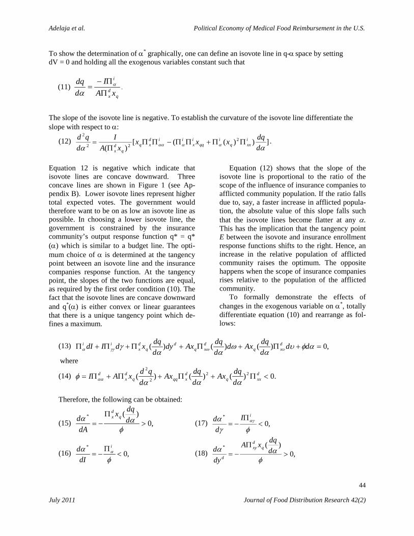
Adelaja et al. Political Economy of Medical Food Reimbursement in the U.S.
44 July 2011 Journal of Food Distribution Research 42(2)
To show the determination of α* graphically, one can define an isovote line in q-α space by setting dV = 0 and holding all the exogenous variables constant such that
(11) q
dx
i
xAI
ddq
ΠΠ−
= α
α.
The slope of the isovote line is negative. To establish the curvature of the isovote line differentiate the slope with respect to α:
(12) ]))(([)(
222
2
αα αααα ddqxxx
xAI
dqd i
xxqi
qqix
iidxq
qdx
ΠΠ+ΠΠ−ΠΠΠ
= .
Equation 12 is negative which indicate that isovote lines are concave downward. Three concave lines are shown in Figure 1 (see Ap-pendix B). Lower isovote lines represent higher total expected votes. The government would therefore want to be on as low an isovote line as possible. In choosing a lower isovote line, the government is constrained by the insurance community’s output response function q* = q* (α) which is similar to a budget line. The opti-mum choice of α is determined at the tangency point between an isovote line and the insurance companies response function. At the tangency point, the slopes of the two functions are equal, as required by the first order condition (10). The fact that the isovote lines are concave downward and q*(α) is either convex or linear guarantees that there is a unique tangency point which de-fines a maximum.
Equation (12) shows that the slope of the
isovote line is proportional to the ratio of the scope of the influence of insurance companies to afflicted community population. If the ratio falls due to, say, a faster increase in afflicted popula-tion, the absolute value of this slope falls such that the isovote lines become flatter at any α. This has the implication that the tangency point E between the isovote and insurance enrollment response functions shifts to the right. Hence, an increase in the relative population of afflicted community raises the optimum. The opposite happens when the scope of insurance companies rises relative to the population of the afflicted community.
To formally demonstrate the effects of changes in the exogenous variable on α*, totally differentiate equation (10) and rearrange as fol-lows:
(13) ,0)()()( =+Π+Π+Π+Π+Π αφυα
ωαα
γ υωγγα ddddqAxd
ddqAxdy
ddqxdIdI d
xqdxq
dq
dx
ii
where
(14) .0)()()( 222
2
<Π+Π+Π+Π= dxxq
dxqqq
dx
d
ddqAx
ddqAx
dqdxAI
αααφ αα
Therefore, the following can be obtained:
(15) ,0)(*
>Π
−=φ
αα ddqx
dAd q
dx
(17) ,0*
<Π
−=φγ
α αγiI
dd
(16) ,0*
<Π
−=φ
α αi
dId (18) ,0
)(*
>Π
−=φ
αα ddqxA
dyd q
dxy
d
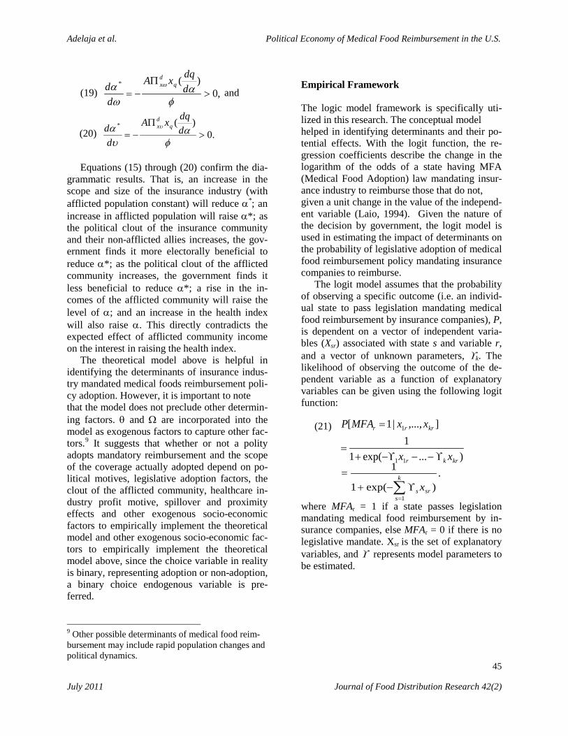
Adelaja et al. Political Economy of Medical Food Reimbursement in the U.S.
45 July 2011 Journal of Food Distribution Research 42(2)
(19) ,0)(*
>Π
−=φ
αωα ω d
dqxA
dd q
dx
and
(20) .0)(*
>Π
−=φ
αυα υ d
dqxA
dd q
dx
Equations (15) through (20) confirm the dia-
grammatic results. That is, an increase in the scope and size of the insurance industry (with afflicted population constant) will reduce α*; an increase in afflicted population will raise α*; as the political clout of the insurance community and their non-afflicted allies increases, the gov-ernment finds it more electorally beneficial to reduce α*; as the political clout of the afflicted community increases, the government finds it less beneficial to reduce α*; a rise in the in-comes of the afflicted community will raise the level of α; and an increase in the health index will also raise α. This directly contradicts the expected effect of afflicted community income on the interest in raising the health index.
The theoretical model above is helpful in identifying the determinants of insurance indus-try mandated medical foods reimbursement poli-cy adoption. However, it is important to note that the model does not preclude other determin-ing factors. θ and Ω are incorporated into the model as exogenous factors to capture other fac-tors.9 It suggests that whether or not a polity adopts mandatory reimbursement and the scope of the coverage actually adopted depend on po-litical motives, legislative adoption factors, the clout of the afflicted community, healthcare in-dustry profit motive, spillover and proximity effects and other exogenous socio-economic factors to empirically implement the theoretical model and other exogenous socio-economic fac-tors to empirically implement the theoretical model above, since the choice variable in reality is binary, representing adoption or non-adoption, a binary choice endogenous variable is pre-ferred.
9 Other possible determinants of medical food reim-bursement may include rapid population changes and political dynamics.
Empirical Framework The logic model framework is specifically uti-lized in this research. The conceptual model helped in identifying determinants and their po-tential effects. With the logit function, the re-gression coefficients describe the change in the logarithm of the odds of a state having MFA (Medical Food Adoption) law mandating insur-ance industry to reimburse those that do not, given a unit change in the value of the independ-ent variable (Laio, 1994). Given the nature of the decision by government, the logit model is used in estimating the impact of determinants on the probability of legislative adoption of medical food reimbursement policy mandating insurance companies to reimburse.
The logit model assumes that the probability of observing a specific outcome (i.e. an individ-ual state to pass legislation mandating medical food reimbursement by insurance companies), P, is dependent on a vector of independent varia-bles (Xsr) associated with state s and variable r, and a vector of unknown parameters, ϒk. The likelihood of observing the outcome of the de-pendent variable as a function of explanatory variables can be given using the following logit function:
(21)
where MFAr = 1 if a state passes legislation mandating medical food reimbursement by in-surance companies, else MFAr = 0 if there is no legislative mandate. Xsr is the set of explanatory variables, and ϒ represents model parameters to be estimated.
)...exp(11
],...,|1[
11
1
krkr
krrr
xx
xxMFAP
ϒ−−−ϒ+=
=
.)exp(1
1=
1∑=
ϒ−+k
ssrs x

Adelaja et al. Political Economy of Medical Food Reimbursement in the U.S.
46 July 2011 Journal of Food Distribution Research 42(2)
11 Phenylketonuria is most common in whites in United States. (http://emedicine.medscape.com/article/947781-overview)
11
To obtain the estimates for explanatory variables in the logit model, the changes in probability, MFAi, brought about by a change in any of the independent variables, Xij, is given by: (22) (∂MFAr / ∂Xsr) = [ϒj exp (-ϒXsr)] /
[1+ exp (-ϒXsr) 2].
Marginal probabilities associated with change in any of the explanatory variables are given by:
(23) (∆MFAi /∆Xsr) = MFAr(Xsr = 1) – Pi(Xsr = 0).
The maximum likelihood function for ex-
pression in (22) can be given as:
(24) ∑ ∑ ∑ ∑= = = =
ϒ−+−ϒ−−
=ϒϒn
i
k
s
n
i
k
rsrjsrsr
k
xXMFA
L
1 1 1 1
1
))exp(1ln()1(
),...,(ln(
Therefore, the specification for medical food
adoption is estimated by a maximum likelihood procedure that generates estimator values by maximizing the log-likelihood function in (24), i.e.,
)).,...,(ln(max))ˆ,...,ˆ(ln( 11 kk LL ϒϒ=ϒϒ Data The data came largely from a survey of the Unites States medical food reimbursement law status which was collected between 1999 and 2003. Relevant parties in all 50 states were con-tacted directly to find out if medical food insur-ance reimbursement laws existed. This was fol-lowed by pulling relevant legislation in these states. Data obtained were used to create a cross-sectional database for the fifty states.10 Other sources of data included U.S. Census, 10 This survey was directed by the primary author and conducted primarily through a special undergraduate research course taught by the primary author and other instructors in 1999. The authors continued the survey effort until 2003. Legislative adoptions through July 2003 were included in the modeling exercise.
Bureau of Labor Statistics and others as depicted in Table 2. Data on independent variables used in the analysis were for the latest year available before state legislative adoption, except in the case of states with no legislation where the data used was for the last year before 2003.
Consider first the political and economic var-iables. To measure the size, strength and politi-cal clout of the afflicted community, the number of existing metabolic clinics in the state (META) and the size of the afflicted community (AF-FLICT) were chosen as proxies. These measures of political clout are consistent with the notion that size, and not percentage, are the prerequisite for coalition. The number of Metabolic and Dis-ease Clinics is hypothesized to positively relate to legislative adoptions. Metabolic clinics pro-vide an area where the afflicted community can gather in numbers for food procurement, pro-moting public awareness and staging lobbying efforts. AFFLICT (AFFLICTSQ) was added to test the hypothesis that at lower levels of afflict-ed population, an increase in the population of the afflicted raises concerns about legislative adoption and lowers the likelihood of adoption, up to the point where the numbers become large enough for the afflicted coalition to form and fight for reimbursement legislation. To measure the political strength and clout of parties oppos-ing medical food reimbursement, the percentage of state residents covered by private insurance companies (PERINSUR) is used. To capture the political structure of the legislature and voters, the percentage of the state legislators that are Democratic (DEMOC) and the percentage of the voting population above 18 (VOTE) were used to test whether democrats are more favorable in their support of families and individuals with medical conditions and whether those over 18 are more likely to support medical food reim-bursement policy.
Now consider the socioeconomic and demo-graphic factors. State’s per capita income (IN-COME) is introduced to measure the affordabil-ity of the medical food expenditure by the public through legislative provision for insurance reim-bursement. Whites Americans have a higher in-cidence rate of certain metabolic diseases like phenylketonia and this could influence the po-litical landscape.

Adelaja et al. Political Economy of Medical Food Reimbursement in the U.S.
47 July 2011 Journal of Food Distribution Research 42(2)
Similarly, state legislators may find it easier to cater to White Americans who dominate the electorate. Hence, the state percentage of White population (WHITE) was included as an explan-atory variable. The percentage of the state’s expenditure on healthcare and hospitals (HEALTHPERCAP) was used as another proxy for income impact and economic burden on the non-afflicted. High health care costs should trig-ger an adverse vote.
Other socioeconomic and demographic fac-tors include the percentage of the population with a high school education (HIGH) and the number of non-fatal illness incidence rate per 100 full-time workers (ILLNESS). HIGH sug-gests greater public awareness and mobilization potential of citizens for government lobbying. ILLNESS provides information on the access to healthcare. Finally, the recent adoption of medi-cal food reimbursement policy in a neighboring
state (NEIGH) is used to proxy the spillover ef-fect on own passage of medical food reim-bursement legislation. Empirical Results Table 3 provides the parameter estimates of equation (21). The model correctly predicted the state of the dependent variables in 86 percent of the states when the actual values were plugged into the predicted model. The chi-square statistic led to the rejected of the null hypothesis that the explanatory variables as a set were insignificant in explaining variation in the dependent variable, at the 0.02 percent level of significance. The McFadden’s R2 result for the model was 0.45, which indicates that 45 percent of the variations in the dependent variable was explained by the model.
Table 2. Description of Independent Variables and Data Sources Variable Name Description of Variable Source Political and Economic Variables
META Number of Metabolic and Disease Clinics Health Directory
AFFLICT Afflicted population in the State U.S. Census Bureau
PERINSUR Percentage of Residents Covered by Private Insurance Companies U.S. Census Bureau
DEMOC Dummy Variable for State Legislature Controlled by Democratic Party
Statistical Abstract of United States
VOTE Percentage of Population above 18 that voted U.S. Census Bureau
Socioeconomic and Demographic Variables
INCOME Per Capita Personal Income U.S. Census Bureau
WHITE Percentage of Total White U.S. Census Bureau
HEALTHPERCAP Per Capita Expenditure on Healthcare U.S. Census Bureau
HIGH Percentage that Completed High School U.S. Census Bureau
ILLNESS Non-fatal Illness incidence rate per 100 full-time workers Bureau of Labor Statistics
Proximity and Time Variables
NEIGH Presence of medical food reimbursement legislation in neighboring state
Direct. Survey

Adelaja et al. Political Economy of Medical Food Reimbursement in the U.S.
48 July 2011 Journal of Food Distribution Research 42(2)
Table 3. Parameter Estimate for Medical Food Reimbursement Model Independent Variable Estimate Standard Error Change in Probability Intercept** -26.496 13.554
Political and Economic Variables META* 0.895 0.522 0.113 AFFLICTED** -0.005 0.002 -0.0006 AFFLICTSQ* 7.92x10⁻⁶ 0.45 x10⁻⁶ 0.99x10⁻⁷ PERINSUR** -0.172 0.152 -0.022 DEMOC 2.463 3.138 - VOTE -0.107 0.094 -
Socioeconomic and Demographic Variables INCOME* 0.001 0.0004 0.0001 WHITE -4.185 6.777 - HEALTHPERCAP** -0.040 0.021 -0.005 HIGH** 0.362 0.191 0.045 ILLNESS 0.267 0.540 -
Proximity and Time Variables NEIGH* 2.306 1.381 0.209 Significance of Chi-square Statistic: 0.002 McFadden's R2: 0.45 *: Significant at the .10 level
**: Significant at the .05 level
**: Significant at the .05 level Marginal effects on probability adoption are not reported for variables where the estimated coefficients are not statistically significant. Prediction Success
Predicted Actual 0 1 Total 0 17 4 21 1 3 26 29 Total 20 30 50 Number of Corrected Predictions= 43 Percent of Corrected Predictions =86
The findings are largely consistent with a
priori expectations. The results suggest that the more metabolic clinics in a state (META), the more likely the state would pass medical food reimbursement legislation. For every metabolic clinic in the state, the chance of medical food reimbursement legislation being enacted in-creases by 11.3 percent. This finding suggests that metabolic clinics are support infrastructure for the afflicted community and reflect the exist-ing political clout of the afflicted community. The large size of the marginal effects of meta-bolic clinics suggests that this is a primary de-terminant of medical foods insurance reim-bursement laws.
The findings regarding the impact of the size of the afflicted community on probability of adoption is captured by AFFLICT and AF-FLICTSQ, the later testing for structural change
in the relationship between the size of the af-flicted community and the likelihood of legisla-tive action to reimburse. The results suggest that as the size of the afflicted community (AF-FLICT) increases, the likelihood of legislative adoption marginally decreases by 0.06 percent, possibly signifying resistance by a more power-ful insurance lobby against a small and perhaps less organized afflicted community.
However, at larger and larger afflicted com-munity sizes, the probability of adoption from a marginal increase in the afflicted community size will actually increase by 0.99x10⁻⁵ percent. This effect reinforces the positive effects of met-abolic clinics. Since the afflicted community has a vested interest in reimbursement and is the driving force to push reimbursement legislation into state legislators’ hands, it is not surprising that the results suggest the afflicted community bears significant weight on the probability of whether medical food reimbursement legislation will pass through state government successfully.
The results suggest that for every one percent of the state covered by private insurance compa-nies (PERINSUR), the likelihood of medical foods insurance reimbursement legislation adop-tion drops by 2.2 percent. The result suggests the

Adelaja et al. Political Economy of Medical Food Reimbursement in the U.S.
49 July 2011 Journal of Food Distribution Research 42(2)
influence of insurance companies on their clien-tele, and that they have a stake in the negative outcome of medical foods insurance reimburse-ment legislation and thus oppose the passage of reimbursement laws.
Both the VOTE and DEMOC political varia-bles were not statistically significant. These re-sults challenge Dye’s voter participation and party affiliation theories. These results can be explained by the fact that the medical foods is-sue is not a major political and voting issue as it affects few non-afflicted individuals. The notion that democrats are more liberal and offer broad welfare enhancing programs (medical foods re-imbursement in this case) is therefore not sup-ported by this study.
The (HEALTHPERCAP) variable captures existing state commitment to public health and state financial support for such care. The finding suggests that for every additional 10 dollar spent per capita on healthcare in a state, the likelihood of medical food reimbursement decreases by 5 percent. In other words, it suggests that the more money a state spends on healthcare per capita, the less likely medical food reimbursement leg-islation will pass. This result suggests that a state already spending a considerable amount on healthcare expenditures and subsidies is less likely to pass additional legislation increasing the total amount of money spent in healthcare.
Income (INCOME) is also a significant de-terminant of legislative adoption. Holding all else constant, a state registering a 100 dollars more per capital income has a 1 percent addi-tional probability to adopt medical foods reim-bursement legislation. The result confirms the income effect on legislative adoption, more so if a given state has a wider per capita income gap compared to the sample average. The coefficient of the white population (WHITE) was not signif-icant, suggesting race is immaterial to legislators when it comes to medical foods.
The likelihood of medical food reimburse-ment increases as the percentage of the state population with a high school education or high-er (HIGH) increases. Hence, those states with higher education levels seem to have the neces-sary intellectual and financial resources to mobi-lize their citizens to press for measures that at-tempt to reimburse medical food. For every 1
percent increase in the percentage of people in a state with high school education, the probability of medical food reimbursement legislation adop-tion increases by 4.5 percent.
Spillover effects of legislative adoption from neighboring states that already adopted the re-imbursement legislation (NEIGH) is an im-portant determinant. If a state is surrounded by other states that already adopted reimbursement legislation, the likelihood of adoption in that state is expected to increase by 20.9 percent. This result provides strong evidence that legisla-tive spillovers have significant relevance to adoption of a program, perhaps due to the visi-bility and noticeability of legislative adoption in neighboring states by state legislators, and per-haps due to yardstick competition against which legislators want to excel. Conclusion This paper is unique in its application of the po-litical economy framework to the emerging area of medical foods and the challenge medical food producers and marketers face in expanding their markets in an environment where policy is a game-changer. Because of the blurred line be-tween food and drugs, medical foods are contro-versial, especially because the adoption of legis-lation mandating reimbursement forces the in-surance industry to incur new costs (payouts) and possibly raise premium levels. While the size of the afflicted community is small in the United States, the resistance of insurance com-panies has been strong and palpable. One of the explanations for the strong resistance of the in-surance industry is the fear that if states open the door for food reimbursement through medical foods, all sorts of things could eventually be re-imbursed. Currently, there are many non-drug substances that confer significant health benefits to the afflicted. Examples include vitamins, cer-tain botanicals, various medicinal plants, and various food substances. Insurance companies have a vested interest in protecting the reim-bursement schedule for their state from what they consider to be frivolous practices in order to maintain profitability and industry integrity.
Confirmation of the political clout and other hypotheses suggest the endogeneity of public

Adelaja et al. Political Economy of Medical Food Reimbursement in the U.S.
50 July 2011 Journal of Food Distribution Research 42(2)
choice even in an area as controversial as medi-cal foods where the afflicted community is lim-ited in number. What is intriguing about medical foods is that despite the small size of the pro-reimbursement movement, more states have passed medical food reimbursement laws than those that have not. Obviously, the role of the metabolic clinics complements the activities of the afflicted community.
While the issues surrounding medical food reimbursement are largely below the radar screen due to the limited size of the afflicted community, these products provide us with a glimpse of what may come as higher and more educated baby-boomers age, pursue healthier diets, and seek food that offer more than nutri-tion. Despite their preventative properties and potential health-care cost benefits, insurance companies have scoffed at reimbursing for ex-penditure on medical foods. This suggests that foods that confer health benefits but are not medical foods would also be opposed by them. On the other hand, it seems likely that baby-boomers will seek coverage for these foods. Given the fact that medical insurance laws are implemented at the state level and they are sub-ject to the demographics and politics of each state, the ultimate determination of what hap-pens to foods at the boundaries of traditional foods and drugs will be made as a consequence of the size and political clout of parties to the coverage debate.
Contentious debates will likely ensue in the future between the demanders of more liberal policies and those that wish to limit medical foods coverage. The fact that the insurance community is experiencing consolidation may suggest more favorable chances for adoption in the future.
Finally, results from this study should inter-est medical foods producers, wholesalers, dis-tributors and marketers. The supply chain of this high technology component of the food industry is checkered at best, largely because legislative adoption is a silver bullet that can help crystalize the distribution system by reducing the cost of the product from what is typically very high to about zero. This creates instantaneous effective demand. The results suggest that medical foods companies can focus their efforts on states with
high income, with a high education of the af-flicted, with fewer health insurance companies, with more metabolic clinics, with high per capita income, with high levels of education and that border other states that have adopted legislation. They may avoid states with high healthcare costs and those that have stronger private insurance tradition. The fact state racial and party compo-sitions are irrelevant suggest that medical foods companies need not employ differential strate-gies due to these factors. We conclude by restat-ing that findings here could be relevant to other food industries where policy plays a major role in the establishment of markets.
References
Aaron H. Looking Backward: 2001-1991 The
History of the Health Care Financing and Re-form Act of 1988. The Brookings Review 2002; 40-45.
Arnold G. Phenylketonuria. February 2009. Available at
http://emedicine.medscape.com/article/947781-overview
Bardach E. The Implementation Game. MIT Press: Cambridge, MA; 1997.
Begu J, Crowe E, Feldman R. Occupational Regulation in the States:
A Causal Model. Journal of Health Politics, Policy and Law 1981; 6; 229-254.
Bistrian B, Blackburn G, Vitale J, Cochran D, Naylor J. Prevalence of Malnutrition in Gen-eral Medical Patients. Journal of the Ameri-can Medical Association 1976; 235; 1567-1570.
Brown M. The Segmented Welfare System: Dis-tributive Conflict and Retrenchment in the United States, 1968-84. In Remaking the Welfare State: Retrenchment and Social Pol-icy in America and Europe, ed. Michael Brown. Temple University Press, Philadelph-ia; 1988.
Browner W, Westenhouse J, Tice J. What if Americans Ate Less Fat? A Quantitative Es-timate of the Effect on Mortality. Journal of the American Medical Association 1991; 265; 3285-3291.
Cedars-Sinai Medical Center. Available at http://www.csmc.edu/2548.html.

Adelaja et al. Political Economy of Medical Food Reimbursement in the U.S.
51 July 2011 Journal of Food Distribution Research 42(2)
Cook F, Barrett E, Popkin S, Constantino E, Kaufnan J. Convergent Perspectives on Social Welfare Policy: The Views from the general Public, Members of Congress, and AFDC Recipients. Center for Urban Affairs and Policy Research (CUAPR), Research Reports, Evanston, IL; 1988.
Coughlin R. Ideology, Public Opinion and Wel-fare Policy: Attitudes toward Taxes and Spending in Industrialized Societies. Univer-sity of California, Institute of International Studies, Berkeley; 1980.
Derthick M. New Towns in Town. Washington, DC: Urban Institute; 1972.
Dye T. Understanding Public Policy (2nd ed.). Englewood Cliffs, Prentice-Hall, NJ; 1975
Dye T. Politics, Economics, and the Public: Pol-icy Outcomes in the American States. Rand McNally, Chicago; 1966.
Edwards G. III. Implementing Public Policy. Congressional Quarterly Press, Washington, DC; 1980.
Food and Drug Administration, CFR. Code of Federal Regulations. U.S. Government Print-ing Office. HHS Publication 21CFR101.9 (2002), Washington, D.C; 2002.
Grogan C. Political–Economic Factors Influenc-ing State Medicaid Policy. Political
Research Quarterly 1994; 47(3); 589–622. Liao T. Interpreting Probability Models: Logit,
probit, and other Generalized Linear Models. Sage Publications, Thousand Oaks, CA; 1994.
Marshall C, Mitchell D, Wirt F. The context of State-Level Policy Formation. Educational Evaluation and Policy Analysis 1986; 8; 347–378.
Miller E. State Health Policy Making Determi-nants, Theory, and Methods: A Synthesis.
Social Science & Medicine 2005; 61; 2639–2657
Mitchell D. Shaping Legislative Decision: Edu-cation Policy and the Social Sciences. D.C. Health, Lexington, MA; 1981.
Nakamura R, Pinderhughes D. Changing Ana-costia: Definition and Implementation. Policy Studies Journal; 1980; 3.
National PKU News.2003. Available at http://www.pkunews.org.
Otles S, Akcicek E. Medical Foods: Scope and Regulations. Journal of Oil Soap
Cosmetics 2002; 51; 58-62. Peltzman S. Toward a more General Theory on
Regulations. Journal of Law and Economics 1976;19; 211–240.
Protash W, Baldassare M. Growth Policies and Community Status: A Test and Modification of Logan’s Theory. Urban Affairs Quarterly 1983;18; 397–412.
Rosenbaum N. Land Use and the Legislatures: The Politics of State Innovation. Urban Insti-tute, Washington, DC; 1976.
Sabatier P, Mazmanian D. Implementation and Public Policy. Scott Foresman, Glencoe, IL; 1983.
Sharkansky I. Regionalism in American politics. Indianapolis, IN: Bobbs-Merrill;1970.
Shingles, R. Class, Status, and Support for Gov-ernment Aid to Disadvantaged
Groups. Journal of Politics 1989; 51(4); 933-62.
Stigler G. The Theory of Economic Regulation. Bell Journal of Economics 1971; 2; 3–21.
The Food Institute. Food Industry Review, 1999. Fairlawn, NJ; 2001.
Tullock G. The Welfare Costs of Tariffs, Mo-nopolies and Theft. Western Economic Jour-nal 1967; 5; 224–232.
U.S. Bureau of the Census. Statistical Abstract of the United States:. (103rd to 123rd ed.). Washington, D.C.
U.S. Congress 100th Congress. Orphan Drug Amendments of 1988.P.L. 100-290. Amendment of Section 526(a)(1) of the Fed-eral Food, Drug and Cosmetic Act, 21 U.S.C. 360bb (ax1). Library of Congress, Washing-ton, DC; 1988.
U.S. Congress 101st Congress. Nutrition Label-ing and Education Act of 1990. P.L. 101-535. Amendment of Section 403 of the Fed-eral Food, Drug and Cosmetic Act, 21 U.S.C. 343. Library of Congress, Washington, DC; 1990.
Van Horn C, Van Meter D. The Implementation of Intergovernmental Policy. In C. Jones & R. Thomas (Eds.), Public Policy Making in a Federal System , 39–62. Sage Publications, Beverly Hills, CA; 1976.

Adelaja et al. Political Economy of Medical Food Reimbursement in the U.S.
52 July 2011 Journal of Food Distribution Research 42(2)
Weekes J. (Ed.) Alternative Medicine: Integra-tion and Coverage (June, Vol. 1, p. 12; Sep-tember, Vol. 2, p. 3). St. Anthony, Reston, VA; 1997.
Zarkin G, Anderson D. Consumer and Producer Responses to Nutrition Label Changes.
American Journal of Agricultural Economics 1992; 74; 1202–1207.
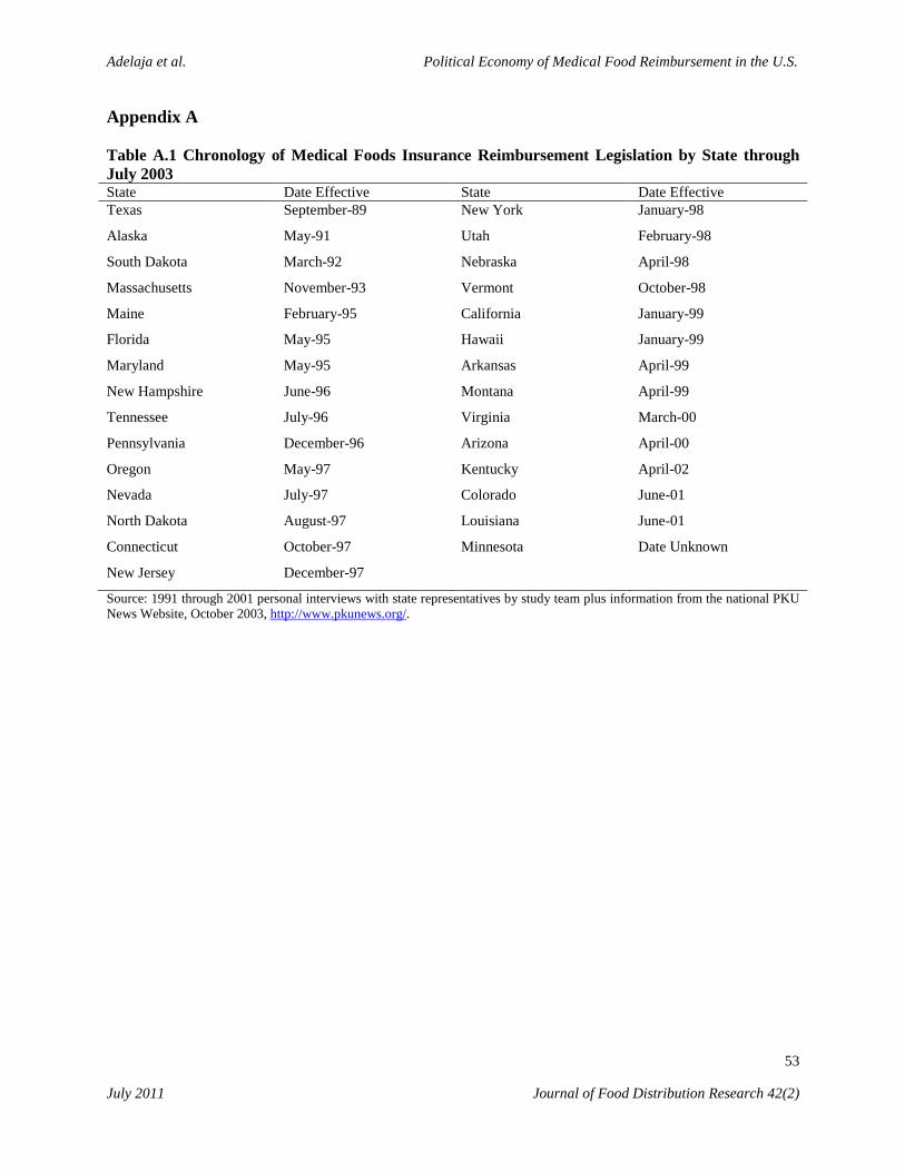
Adelaja et al. Political Economy of Medical Food Reimbursement in the U.S.
53 July 2011 Journal of Food Distribution Research 42(2)
Appendix A Table A.1 Chronology of Medical Foods Insurance Reimbursement Legislation by State through July 2003 State Date Effective State Date Effective Texas September-89 New York January-98
Alaska May-91 Utah February-98
South Dakota March-92 Nebraska April-98
Massachusetts November-93 Vermont October-98
Maine February-95 California January-99
Florida May-95 Hawaii January-99
Maryland May-95 Arkansas April-99
New Hampshire June-96 Montana April-99
Tennessee July-96 Virginia March-00
Pennsylvania December-96 Arizona April-00
Oregon May-97 Kentucky April-02
Nevada July-97 Colorado June-01
North Dakota August-97 Louisiana June-01
Connecticut October-97 Minnesota Date Unknown
New Jersey December-97
Source: 1991 through 2001 personal interviews with state representatives by study team plus information from the national PKU News Website, October 2003, http://www.pkunews.org/.

Adelaja et al. Political Economy of Medical Food Reimbursement in the U.S.
54 July 2011 Journal of Food Distribution Research 42(2)
Table A.2 Criteria for Medical Foods Insurance Reimbursement Across the United States as of July 2003. State Additional
metabolic disorders
Annual dollar limit
Age Limit State Additional metabolic disorders
Annual dollar limit
Age Limit
Alabama - - - Montana* All No No Alaska* None No No Nebraska* Select 2,000 No Arizona* Select 2,500 No Nevada* Select 2,500 21
Arkansas* None 2,400 No New Hamp-shire* Select 1,800 No
California* All No No New Jersey* All No No Colorado* All No 21/251 New Mexico - - - Connecticut* Select No No New York* All 2,500 No
Delaware - - - North Caroli-na* - - -
Florida* Select 2,500 24 North Dakota* MSUD 3,000 No Georgia - - - Ohio - - - Hawaii* All No No Oklahoma - - - Idaho - - - Oregon* All No No Illinois - - - Pennsylvania* MSUD No 21 Indiana - - - Rhode Island - - - Iowa - - - South Carolina - - - Kansas - - - South Dakota* Unknown2 No No Kentucky* All 4,000 No Tennessee* Select3 No No Louisiana* All 2,400 No Texas* Select 3,500 No Maine* Select 3,000 18 Utah* Select No No Maryland* Select No No Vermont* Unknown 2,500 No Massachusetts* Select 2,500 No Virginia* Unknown 2,000 18 Michigan - - - Washington* - - - Minnesota* - - - West Virginia* - - - Mississippi* - - - Wisconsin* - - - Missouri* - - - Wyoming - - - Note: * indicates states with insurance reimbursement for phenylketonuria while - indicates otherwise. Colorado limits vary with age - 21 for males and 35 for females; for states labeled “Unknown”, there exists no interpretive state legislation on addi-tional metabolic disorder coverage. For states labeled Select, only select metabolic disorders are covered. Source: Personal interviews with State Representatives and information from the National PKU News website, October 2003, http://www.pkunews.org/.

Adelaja et al. Political Economy of Medical Food Reimbursement in the U.S.
55 July 2011 Journal of Food Distribution Research 42(2)
Table A.3 Timeline of Federal Policies and Regulations Related to Medical Food
Year
Activity/Legislator 1906 Passage of the Pure Food and Drug Act.
1938 Passage of the federal Food, Drug and Cosmetic Act, regarding medical food as prescription drugs to assure that their use would be supervised by physicians and to prevent misuse by individuals.
1972 FDA revised its classification of medical food from "drugs" to "special dietary food" (21 CFR 105.3).
1973 The FDA defined medical food in 21 CFR 101.9(h)(4) as "food represented for use solely under medi-cal supervision to meet nutritional requirements in specific medical conditions."
1976 The Proxmire Amendment to the FD&C Act (Section 411) differentiated regulation of vitamin and mineral supplements from medical food.
1980 Congress passed the Infant Formula Act (FD&C Act, Section 412), which led to specific regulations (21 CFR 107.10 wt seq.) for the manufacturing of infant formula.
1988 FDA initiated a Compliance Program to enable the agency to evaluate how the medical food industry ensures proper formulation, appropriate microbiological standards, and reasonable therapeutic claims for these products. Passage of the Orphan Drug Act. Congress amended the Drug Act to include the first legal definition of medical food (21 U.S. Code 360ee (b)(3))
1990 The definition for medical food in the U.S. was incorporated into the Nutrition Labeling and Education Act of 1990, (NLEA) (P.L. 101-535) (21 U.S. Code 343) The NLEA, however, exempted medical food from the requirements of nutrition labeling to ensure that other specific regulations would be developed to control medical food.
1991 The Codex Alimentarius Commission approved standards for food for special medical dietary uses.
1994 The passage of the Dietary Supplement Health and Education Act, which expanded the vitamin-mineral category to include herbs, botanicals, proteins, extracts, and metabolites and renamed them as dietary supplements. It also allowed for structure function claims.
1995 The FDA announced the agency’s general policy on the development and use of standards with respect to international harmonization of regulatory requirements and guidelines
2001 The FDA issued Food Compliance Program – “Medical Food – Import and Domestic” which provides regulations on the quality control standards and procedures for medical food.
Appendix B
α
q*
q
α* 0
E V2
V1
V0
q(.)
Figure 1. Optimal Level of Medical Food Reimbursement Protection

56
Consumer Perceptions of Environmentally Friendly Products in New Foundland and Labrador Morteza Haghiri A stated-preference model was specified by a logit model to analyze consumers’ willingness-to-pay a five-per cent premium to purchase environmentally friendly products in Newfoundland and Labrador. Although the industry suf-fers from insufficient number of certified producers in the region, the findings from the model reflect the existence of potential demands for environmentally friendly products. Results showed that survey respondents were willing to pay at least a five-per cent premium, as they believed pesticide residues would have negative impacts on their health conditions. In addition, being married, higher degree of education, knowledge about new methods of farming prac-tices, such as integrated-pest management, and early adopters in trying newly introduced products were among the factors affecting consumer decisions in paying the premium.
Environmentally friendly products (EFPs) are produced without the use of pesticides, herb-icides, chemical fertilizers, antibiotics, and arti-ficial animal growth hormones in any stages of the production. In the case of EFPs sustainability and the ecological balance of natural resources in their production processes are assumed to be as important as the quantity of products. The main objective of producing EFPs is to optimize the overall productivity of scarce resources while considering the fitness of diverse commu-nities within the agroecosystem including soil organisms, plants, livestock and people. To do this, policy makers and market analysts have been trying to define new strategies that lead to a development of new farms that are sustainable and harmonious with the environment (Agricul-ture and Agri-Food Canada, 2005). The idea of producing EFPs has been strengthened by the recent increase of public concerns and favors toward the production, consumption, and distri-bution of these groups of products. As a result, the market for EFPs has been dramatically in-creased in Canada since the beginning of 1990 and its growth is predicted to be increased stead-ily in the future. The environmentally friendly crop production is growing worldwide with an Morteza Haghiri is an Associate Professor of Economics at Memorial University-Corner Brook in Newfoundland, and Labrador, Canada.
The author would like to thank the Centre of Environ-mental Excellence (CEE) at the Memorial University of Newfoundland and Labrador at Corner Brook that provides funding for this research. The views expressed in this paper are those of the author and are not those of the Centre of Environmental Excellence.
annual turnover of more than $US25 billion of-fering a range of market opportunities for these group of farmers. This has been a significant movement from the 1980s when the industry was recognized as a niche market.
Canada then is an appropriate country for producing EFPs because of its large land base and its mainly intemperate climate, which to-gether tend to reduce various plant disease and pest problems. In 2004, more than 1.2 million acres of arable land in Canada were allocated to grow EFPs. It was also predicted that additional 141,000 acres were in transition to be cultivated under these groups of products (Macey, 2005). Evidence shows that the number of certified producers who commercially grew EFPs have been increasing significantly from 2002 to 2004 in the country. In 2002, there were a total of 3,120 certified farms producing EFPs while this figure was raised to 3,670 in 2004; an average increase of 8.1 per cent per year (Macey, 2004). Nevertheless, it only represents 1.5 per cent of total farms in Canada if the Census of Agricul-ture in 2001 is considered as the base year (Sta-tistics Canada, 2001).
The Canada’s crop map displays that EFPs are dispersedly grown in the country, given their bioregional characteristics. For example, envi-ronmentally friendly grains and oilseeds are mainly produced in the Prairies, whereas dairy products in Quebec and Ontario, fruits in British Columbia, and fresh vegetables and herbs, for-ages, permanent pastures, and green manure crops are grown in all provinces. Moreover, At-lantic Canada and Quebec are the center of berry

Haghiri Consumer Perceptions of Environmentally Friendly Products in Newfoundland and Labrador
57 July 2011 Journal of Food Distribution Research 42(2)
production including cranberries and wild har-vested blueberries.
Macey (2005) reported that total value of EFPs in Canada was ranged between 250 to 350 million dollars. Most of the Canada’s EFPs is exported to France, Germany, Italy, the United Kingdom, Japan, and the United States. Among them, grains and oilseeds have great share in Canada’s total exported products. Of the $65 million of Canada’s total exported EFPs in 2005, wheat was in the first place with an estimated value of 14 million dollars (Agriculture and Agri-Food Canada, 2005). Since Canada cannot produce all types of EFPs (e.g., bananas and cit-rus fruits), more than 75 per cent of households’ consumption of these types of products are pro-vided from the foreign markets. It is predicted that the industry would increase its domestic retail market share to 10 per cent by 2010.
Despite the increase in the area under cultiva-tion of EFPs, producers in Atlantic Canada have not yet responded appropriately to meet the on-going increase in the demand for EFPs. In 2004, there were only 115 certified environmentally friendly producers in Atlantic Canada. Of these, only four producers (three farms active and one farm in transition) were operating in the prov-ince of Newfoundland and Labrador (Macey, 2005). Moreover, there were at least 79 acres of arable land were under the cultivation of envi-ronmentally friendly production (vegetables and blueberries) and 30 acres were in transitions in the same year (Macey, 2005). Although these figures demonstrate that the industry is underde-veloped in the province it does not necessarily mean that the demand for EFPs do not exist. There is not much information on the consumer market for EFPs in Newfoundland and Labrador. Studies like this research will help regional poli-cy makers, market developers, investors, proces-sors, handlers, traders, and environmentally friendly producers recognize the availability of demands for EFPs in the province.
The objectives of this paper are two-fold. First, to find the availability of the demand for EFPs in Newfoundland and Labrador we identi-fy factors motivating consumers to purchase EFPs. The production cost of EFPs is usually higher than that of the conventional agricultural products (Govindasamy and Italia, 1999). This
difference, known as the premium, would there-fore be passed onto the consumers. The amount of the premium depends on the EFPs prices and the demand drivers including consumers’ in-come, tastes and preferences, and the prices of related products. The amount of the premium ranges from five to 25 per cent and varies re-gionally on a product basis. Second, we use the concept of willingness-to-pay (WTP) the premi-um as a way of maximizing consumer’s satisfac-tion to examine the impact of factors affecting Newfoundlanders and Labradorians’ decisions to purchase EFPs in the market. The WTP is modeled through a binary-choice logit frame-work as a function of a series of independent continuous and dummy variables including so-cio-demographic, socio-economic, media, and public perceptions toward EFPs.
The rest of the paper is organized as follows. Next section provides recent studies in Canada in which consumers’ WTP are examined fol-lowed by a brief review on the binary-choice logit models. The sections following present a summary of data collected from the consumer survey, a justification for the selection of inde-pendent variables, and a discussion of the re-sults. The final section concludes the paper, pre-sents some policy implications, and introduces further research topics required advancing this analysis.
Recent Studies on EFPs in Canada
Few studies in Canada investigated consumer perceptions on EFPs in the recent decade. Here we review only those studies whose methodolo-gies and dependent and independent variables are similar to those of this study to avoid biased outcomes in comparing findings.
Veeman and Adamowicz (2001) conducted a research to examine consumer perceptions of environmental risks and the demand for food safety in Alberta. They used the contingent val-ue method to assess Albertans’ purchasing be-havior towards EFPs raised from a range of en-vironmental risks, such as pesticide residues arisen in conventional agricultural foods and hormonal treatments derived from biotechnolog-ical farming practices. The result showed that consumers in Alberta were less susceptible to-

Haghiri Consumer Perceptions of Environmentally Friendly Products in Newfoundland and Labrador
58 July 2011 Journal of Food Distribution Research 42(2)
wards the use of hormones than the use of pesti-cide in the food production. In addition, being female and higher levels of education and in-come had positive effects on the WTP a premi-um, ranged from 13 to 25 per cent, to purchase EFPs. Veeman and Adamowicz (2001) also used a conditional logit model of consumer choice to examine Albertan’s purchasing behavior to-wards the consumption of milk produced by us-ing the recombinant bovine somatotrophin (rBST) in the production process. They consid-ered other characteristics including fat content, price, and freshness as well as the use of rBST identified by labeling. Since the use of rBST in Canada is prohibited the objective of the re-search was to simulate market conditions and consumer responses towards a twofold scenari-os: production milk with and without the use of rBST. The result showed that consumers were worse-off with the introduction of rBST. The losses were less for male than that of female households and for those consumers with higher levels of income and education. A small welfare gain was identified when households were of-fered a full range of rBST and non-rBST milk. The researchers concluded that consumers could abate their welfare losses if the produced milk labeled “rBST-free” milk.
Using the contingent valuation method Cran-field and Magnusson (2003) classified Canadian consumers based on the degree of their ac-ceptance toward the consumption of pesticide-free products. The degree of acceptance of these groups of EFPs was measured by how much ex-tra money consumers would like to spend on pesticide-free products than of what they nor-mally pay for non-pesticide-free products. The result showed that 67 per cent of the sample ob-servations were willing to pay the premium ranged from one to 10 per cent and only five per cent of the respondents tended to pay a premium of 20 per cent over conventional food prices.
Larue et al. (2004) collected data from a sample of 1,008 consumers to analyze their re-sponses to buy various foods produced by dif-ferent methods of production including conven-tional, organic, and genetically modified proce-dures. The researchers chose chicken breast, to-mato sauce, and potato chips to assess an expan-sion of organic nich food markets for a combina-
tion of organic tomato sauce and organic chick-en breasts. Larue et al. (2004) hypothesized that households would consume these products for their sanitary characteristics including anti-cancer for tomato sauce and heart-healthy for chicken breast. The researchers failed to reject their hypothesis implying that households would be willing to pay additional money to purchase organic tomato sauce and organic chicken breast as long as sanitary properties are attached to the-se products.
The assessment of market demand for a group of pesticide-free products including pasta, breakfast cereal, dry peas, sunflower seed, beer, multigrain bread, canola oil, and dry lentils was the main objective of a research conducted by Magnusson and Cranfield in 2005. Using a pro-bit model, the researchers found that some so-cio-demographic, socio-economic, and market-oriented factors, such as switching grocery stores to purchase pesticide-free products, being less than 36 years of age, and high level of household income could have potentially impact on consumer decisions to purchase the pesticide-free products.
The review studies show that consumers are willing to pay a premium, which varies from one region to another, to purchase EFPs as long as they believe the use of pesticide and chemical materials would seriously affect their health condition and environment. This will certainly open a new era for environmental friendly pro-ducers to identify different market segments in each region. The production of EFPs has not yet been developed in Newfoundland and Labrador. Several reasons may justify the lack of farmers’ interests in growing these types of products. These reasons are climatological conditions, lack of liquidity for farmers, resistance to adopt new technology, and finally the lack of infor-mation on the demand side in the province. This paper will draw on these insights to develop a methodology for assessing consumer prefer-ences for EFPs in Newfoundland and Labrador.
Methodology
We used a binary-choice logit model whose pa-rameters are estimated by the maximum-likelihood (ML) technique. Logit models are
Haghiri Consumer Perceptions of Environmentally Friendly Products in Newfoundland and Labrador
59 July 2011 Journal of Food Distribution Research 42(2)
widely used in the consumer survey studies be-cause their asymptotic properties guarantee the predicted probabilities to be in the range of zero to one (Greene, 2008). In a likelihood function, a joint probability density function of dependent variables nYYY ,...,, 21 is constructed as inde-pendent variables that are randomly derived from a Bernoulli distribution with probabil-ity iπ , which varies from one observation to another. The expected value of the dependent random variable and its variance, respectively, is ( ) [ ] iii 1YYE π=== Pr and ( ) ( ). Var iii 1Y π−π=
We assume a positive outcome as a probabil-
ity of observing a success derived from the be-havior of a representative consumer who is will-ing to pay at least a five-percent premium to purchase EFPs. The probability of success is ( )ii X π=π in which iX represents a vector of independent variables including demographic characteristics, socio-economic variables, media factors, and public awareness of hazardous on health condition and environment involved with the consumption of agricultural products that are produced from conventional farming practices. The five per cent premium is drawn from the information collected from the sample observa-tions in the survey. Since the probability of suc-cess ranges from zero to one, the value of ( )⋅π falls in the unit interval (0,1). Therefore, we can write the probability of success as
(1) ( ) ( )
) ( exp1) ( exp
γ
γγ
i
iiii X
XX′+
′=′Λ=ΩΛ=π
in which iΩ represents the information set con-sisting of independent variables, γ iX ′ is the index function that maps a linear combination of independent variables from the covariate vector
iX and the vector of unknown parameters γ , and ( )iΩΛ is the value of the logistic cumula-tive density function. In light of this, equation [2] specifies a logit model
(2)
,...1
log 22110 εγγγγπ
π+++++=′=
−
=Ω nnii
ii xxxγX
ni ,...,2 ,1= that iΩ represents the log odds of choice for
the ith observation, ix indicates the ith independ-ent variable associated with each dependent var-iable, nγγ ,...,1 are the unknown parameters that must be estimated, and ε is the random error term. The signs of the estimated parameters in equation [2] will show the direct impact of a change in any of the explanatory variables on the probability of a success ( )1=Y quantified by the marginal effects (ME). Equation [3]
measures the ME of the thj independent variable on the probability of a success, (3)
( ) ( )
( )[ ]2 exp1
expscale where * scale
1
γ
γ
i
ij
ij
iix
xY
X
X′+
′=γ=
∂=π∂
In practice, the impact of MEs is evaluated at
the sample mean for continuous independent variables, whereas equation [4] is used when the explanatory variables are either discrete varia-bles or dummies.
(4)
( ) ( )ΘΘ ==π−==π XxYXxY jj ,0 1 ,1 1
In equation [4], ΘX is defined by setting all
dummy variables to their modal values and all continuous independent variables to their mean values. Equation [4] calculates the change in the probability of a success ( )1=Y yielding from a change in jx between zero and one, holding all
other variables at some fixed values ΘX . To predict a representative consumer’s WTP
at least a five per cent premium to purchase EFPs in the region of the study, we developed the following regression model:

Haghiri Consumer Perceptions of Environmentally Friendly Products in Newfoundland and Labrador
60 July 2011 Journal of Food Distribution Research 42(2)
(5)
Prior to estimate equation [5], we dropped
one category from each of the group-category independent variables to avoid the perfect col-linearity in the model (see Table 1). It is ex-pected that consumers with higher levels of in-come or education are more likely to pay the premium. In addition, respondents who have seriously concerns about the status of health and the environment will tend to purchase EFPs.
Empirical Analysis Data Description
To analyze consumers’ WTP to purchase EFPs, we elicited a consumer survey using a stated preference methodology during winter 2007 in the province of Newfoundland and Labrador. In particular, sample observations were randomly selected from St. John’s, Mount Pearl and Grand-Falls Windsor in the east, and Deer Lake, Pasadena, Corner Brook, and Port aux Basque in the west of the province. The survey was con-ducted during weekday and weekend periods in various time of the day. We set up a table in shopping centers, handed in a two-page ques-tionnaire to each one of the participants ap-proaching the table, and collected the question-naires in the same day. To minimize bias in sampling, participants were told the purpose of the survey was about their perceptions towards the consumption of various foods in general without mentioning the term EFPs. Prior to completing the survey, participants were given a one-page “consent and contact” letter that de-scribes the objectives of the research and em-phasizes that their contribution is completely voluntarily and they can quit the survey at any time.
We are aware of the limitations facing stud-ies in which the stated preference methodology is selected as the focus of the research. x
Consumer survey studies are usually time-and-location variant that might cause an inaccurate collection of information received from re-spondents. Nevertheless, such research as being done here still yields useful information and contributes to the body of literature. The ques-tionnaire was designed based on what Govindasamy et al (2001) and Hobbs et al (2005) used in their studies with slight changes made to reflect the characteristics of the region. Due to the budget limitations the survey was not conducted in Labrador. In total, 447 individuals were approached and 222 completed question-naires were collected, yielding a 49.6 per cent response rate. Of these, 108 questionnaires were completed in eastern Newfoundland and the rest (51.3 per cent) was completed in the west part of the province. Prior to the main survey, we tested the model in a small scale in Corner Brook and its suburbs, and excluded the results of the pilot survey from the final analysis.
Table 1 presents a descriptive analysis of the variables used in the study. Of the 222 total number of survey participants, 45 per cent were male and the rest were females, which, to some extent, conforms to the 2006 Census Provincial Population in which 49.5 per cent of the resi-dents in NL was male and 50.5 per cent was fe-males (Statistics Canada, 2007). The survey showed that 63.1 per cent of the participants were between 31 to 60 years of age and 33 per cent of them were singles. In addition, more than 70 per cent of the respondents declared that they had either a college or a university degree. The result also showed that near 42 per cent of the survey respondents earned an annual income between $30,000 to less than $50,000, whereas only seven per cent reported an annual house-hold income of more than $80,000. Table 1 dis-plays that the annual household income of near 75.2 per cent of the survey participants was less than $50,000. This implies that the information drawn from the sample observations conform to
, 4 3
2 3 2 4 3 2 2 4 3 2
242322212019
181716151413
121110987
6543210
εγγγγγγγγγγγγγγγγγγ
γγγγγγγ
++++++++++++
+++++++++++++=
locartimedipmpsenpshtrnewpurogvisfmvisgincinc
incempempedueduedufszmaritageageagegenWTPEFPs

Haghiri Consumer Perceptions of Environmentally Friendly Products in Newfoundland and Labrador
61 July 2011 Journal of Food Distribution Research 42(2)
the data released by Statistics Canada in 2006 indicating that the annual per capita income in the province of Newfoundland and Labrador was $31, 234 (Statistics Canada, 2007).
Table 1 (See Appendix A) shows that 64 per cent of the survey respondents visited grocery stores to purchase advertised products and 63 per cent visited farmers’ markets in the past five years. In total, more than 74 per cent of the par-ticipants believed that the use of pesticides poses a serious risk to human health, and 81.1 per cent thought that the use of various pesticides has negative impacts on the environment. Of the 222 sample observations, 22 per cent knew about the integrated-pest management as one of the new methods of farming practices prior to this sur-vey. Finally, 49 per cent of the respondents ex-pressed that they saw on television or heard from radio few programs aired about EFPs and 33 per cent declared that they had read articles about these types of products in magazines and newspapers, and on-line. Overall, 66.2 per cent of the survey participants stated that they were willing to pay at least a five-per cent premium to purchase EFPs. Since the majority of the survey respondents chose such a percentage, the five per cent premium was used to specify the de-pendent variable. Estimation Results
Table 2 displays the estimation results of the logit model used to analyze consumers’ choices by paying five per cent more than what they used to pay for conventional food to purchase EFPs in the province of Newfoundland and Lab-rador. The parameters of the regression model were estimated through the ML approach by using NLOGIT (Version 3.0). In the model, the dependent variable (WTPEFPs) was coded as 1 indicating a representative consumer’s WTP the five per cent premium for EFPs and zero other-wise. Overall, using the likelihood ratio (LR) statistic test, the calculated chi-square statistic was found to be 164.6, which rejects the null hypothesis that all slope coefficients were zero at the 0.01 level of significance. The Pseudo R–squared figure (0.5769) also represents a reason-able goodness-of-fit for the entire regression model although as Pindyck and Rubinfeld
(2000) expressed that binary choice models with cross sectional data are not expected to be esti-mated with high R-squared values.
Table 2 shows that married people (MA-RIT2) were 30 per cent more likely to pay a five-per cent premium to purchase EFPs than that of singles in the province. The MARIT2 variable was positive and statistically significant at the 0.06 level. The result indicates that the level of education is positively related to the consumption of EFPs. Evidence shows that as respondents have higher level of education, they are more likely to pay the premium to purchase EFPs. Table 2 shows those respondents holding an undergraduate degree (EDU3) were 20 per cent more likely to pay the five-per cent premi-um than that of people with a high school degree to buy EFPs. The coefficient of EDU3 was posi-tive and statistically significant at the 0.05 level. In addition, respondents with a graduate degree (EDU4) were 17 per cent more likely to pay the premium when compared to those holding a high school diploma or those who did not finish high school. This is shown by the partial slope coeffi-cient of EDU4 that was positive and statistically significant with 99 per cent confidence. These results support those of Magnusson and Cran-field (2005), but in contrast with what Go-vindasamy and Italia (1999) and Boccaletti and Nardella (2000) reported. This comparison would not be feasible if the dependent and inde-pendent variables used in the studies were not similar to each other.
The dummy variable indicating that the re-spondents usually consider EFPs in their basket of foods (PUREFPs) was positive and statisti-cally significant with 99 per cent confidence. The magnitude of the coefficient was 0.5077 implying that these group of consumers were approximately 51 per cent more likely to pay at least a five-per cent premium to purchase EFPs than those who did not tend to buy these types of products. Other studies also reported similar consumer behavior towards the consumption of EFPs (see, e.g., Govindasamy and Italia, 1999; and Batte et al., 2004). Batte et al. (2004, p.14) expressed that consumers who were willing to pay a premium to purchase EFPs were usually less concern about the prices of these products. We observed similar consumer behavior, but

Haghiri Consumer Perceptions of Environmentally Friendly Products in Newfoundland and Labrador
62 July 2011 Journal of Food Distribution Research 42(2)
Table 2. Estimation Results
* Significant at 0.10, ** Significant at 0.05, *** Significant at 0.01.
with a mitigated reflection in the region of the study. The dummy variable denoting whether individuals classify themselves as among the very first to try newly introduced food products (TRNEW) was positive and statistically signifi-cant with a p-value of 0.0089. This implies that, everything else being equal, these groups of re-spondents were 20 per cent more likely to pay a five-per cent premium to buy EFPs than those who were not classified themselves as first-adopter consumers.
Table 2 shows that the independent dummy variable representing the participants’ concerns
about the use of pesticide in farming practices and its effects on their health condition (PSH) was positive and significant at the 0.06 level. The magnitude of the estimate of the PSH vari-able was 0.3142 implying that environmentally friendly consumers, on average, were 31 per cent more likely to pay the premium than those of nonbelievers in the adverse effects of the conventional food products. This finding support those reported by Haghiri et al. (2006). The last explanatory variable that was statistically signif-icant at the 0.05 level was the public knowledge about the new method of agricultural farming
Variable name Estimate (p-value)
Change in Probability (p-value)
Constant *** -3.9341 (0.0029) -0.5091 (0.0167) GEN -0.0738 (0.9036) -0.0095 (0.9035) AGE2 -0.3753 (0.6556) -0.0501 (0.6677) AGE3 -1.1628 (0.3052) -0.1827 (0.3850) AGE4 -0.1001 (0.9446) -0.0132 (0.9460) MARIT2 * 1.8559 (0.0362) 0.2959 (0.0633) FSZ -0.3458 (0.1569) -0.0447 (0.1581) EDU2 0.4852 (0.4318) 0.0591 (0.4159) EDU3 ** 1.7143 (0.0317) 0.2000 (0.0303) EDU4 *** 2.6338 (0.0738) 0.1682 (0.0033) EMP2 0.4543 (0.5470) 0.0633 (0.5796) EMP3 0.4558 (0.7212) 0.0523 (0.6885) INC2 0.0995 (0.8697) 0.0128 (0.8692) INC3 -0.1185 (0.9065) -0.0157 (0.9089) INC4 -0.3465 (0.8210) -0.0496 (0.8383) VISG -0.8805 (0.1463) -0.1053 (0.1147) VISFM 0.1476 (0.8112) 0.0193 (0.8145) PUREFPs*** 3.4867 (0.0000) 0.5077 (0.0000) TRNEW *** 1.6999 (0.0089) 0.2016 (0.0047) PSH * 1.8381 (0.0217) 0.3142 (0.0623) PSEN -0.1561 (0.8351) -0.0195 (0.8294) IPM ** 1.1017 (0.1055) 0.1159 (0.0459) MED 0.7099 (0.2054) 0.0918 (0.2009) ARTI 0.6344 (0.2760) 0.0765 (0.2679) LOC 0.5138 (0.3625) 0.0669 (0.3857) Number of observations 222 McFadden R-squared (Pseudo R–squared) 0.57698 Likelihood ratio statistic 164.6154 Degrees of freedom 24 Prob [ChiSqd > value] 0.0000

Haghiri Consumer Perceptions of Environmentally Friendly Products in Newfoundland and Labrador
63 July 2011 Journal of Food Distribution Research 42(2)
practices, known as the integrated-pest man-agement (IPM). This method of farming prac-tice is an ecosystem-based method used to con-trol pests and weeds through a series of different techniques, which are least injurious to the envi-ronment and most specific to the particular pest and weed. The IPM method includes biological control, habitat manipulation, modification of cultural practices, and the use of pest resistant plant varieties. The result shows that respond-ents having knowledge of IPM are 12 per cent more likely to pay the premium to purchase EFPs when compared to those who did not know anything about new method of farming practices
Finally, we examined the effects of other var-iables on the WTP the premium to purchase EFPs in the model and found none of them was statistically significant. These variables were gender, age, family size, income levels, em-ployment status, visiting grocery stores and farmers’ markets, believed in the negative im-pact of synthetic pesticides use on environment, media, articles read about EFPs, and location.
Table 3 presents the frequencies of actual and predicted outcomes. Overall, the estimated re-gression model correctly identified 198 observa-tions out of 222 total sample of observations (89.2 per cent). However, the correct percentage of predictions against the naive predictions (herein, all one) is 65.7 per cent of the total ob-servations (146/222), suggesting a reasonable prediction.
Table 3. Frequencies of Actual and Predicted Outcomesa
Predicted
Actual 0 1 Correct
0 63 13 63/76 1 11 135 135/146
a Total number of observations: 222. Total number of correct predictions: 198
Conclusion and Suggestions for Managers
The recent global appearance of a series of communicable diseases including Avian Flu, Bovine Spongiform Encephalopathy, and Poly-chlorinated Biphenyls in Atlantic farmed salmon have affected human lives especially infants, young children, and the elderly people world-wide. To date, the food incidence of salmonella
outbreak in Mexican tomatoes has not been solved and attentions have now been made to-ward Mexican cilantro and peppers. In addition, the existence of harmful microorganisms, agri-cultural chemicals, non-tested GM foods, and the misrepresentation of food origin placed a level of distrust in the food markets. As a result, households concern seriously about the quality of food they consume. The fear of being exposed by adverse effects of consuming conventional food on health and environment has brought substantial motivations for consumers to in-crease their demands for EFPs in the province of Newfoundland and Labrador.
The production of EFPs needs to be expand-ed in Newfoundland and Labrador. The lack of a developed sector of producing these groups of products can be imputed to several reasons; none of them stems from the demand side. The lower amount of the premium, which has lessened the motivations of producers and distributors of EFPs to increase their production scale, is one reason why the industry has not been developed.
Several points are drawn from the results of this study. First, different level of market seg-ments for EFPs are available among consumers in Newfoundland and Labrador. Second, the martial status and high level of education have positive relationships with willingness-to-pay the premium strengthened by the public aware-ness of new farming methods including integrat-ed-pest management. Third, consumers favor their health status against environment when making decisions to purchase EFPs. Fourth, a tendency toward the consumption of newly in-troduced products among consumers has been observed as the estimated parameter of the mod-el was translated in paying the premium.
Due to the structure of the research we were unable to measure the sensitivity of consumers’ decisions to pay the premium with respect to the changes in the levels of incomes and the EFPs prices. Thus, further studies are suggested to estimate the price and income elasticities of de-mands for EFPs. In addition, to encourage pro-ducers to grow EFPs, the provincial government should implement appropriate policies in support of the industry so that certified producers will have cost advantages in producing these types of products and as a result they will be become
Haghiri Consumer Perceptions of Environmentally Friendly Products in Newfoundland and Labrador
64 July 2011 Journal of Food Distribution Research 42(2)
more competitive in Canada. Meanwhile, public awareness of the advantages of consuming EFPs should be steadily raised. The aid of media (ra-dio, television, and newspapers) in promoting the consumption of EFPs will help the industry grow consistently.
References Agriculture and Agri-Food Canada.
2005.“Canada’s Agriculture, Food and Beverage Industry.” Ottawa, Ontario.
Batte, M. T., J. Beaverson, N. H. Hooker and T. Haab. 2004. “Customer Willingness-to-Pay for Multi-Ingredient, Processed Organic Food Products.” The Annual Meeting of the American Agricultural Economics Associa-tion, Denver, Colorado, (July).
Boccaletti, S. and M. Nardella. 2000.“Consumer Willingness-to-Pay for Pesticide-Free Fresh Fruit and Vegetables in Italy.” International Food and Agribusiness Management Review 3:297-310.
Cranfield, J. A. L. and E. Magnusson. 2003. “Canadian Consumers’ Willingness-to-Pay for Pesticide Free Food Products:An Ordered Probit Analysis.” International Food and Agribusiness Management Review 6 (4):13-30.
Govindasamy, R. and J. Italia. 1999. “Predicting Willingness-to-Pay a Premium for Organi-cally Grown Fresh Produce.” Journal of Food Distribution Research 30(2):44-53.
Govindasamy, R., J. Italia and A. Adelaja. 2001. “Predicting Willingness-to-Pay a Premium for Integrated Pest Management Produce: A Logistic Approach.” Agricultural and Re-source Economics Review 30(2):151-159.
Greene, W.H. 2008. Econometric Analysis. 6th edition. New Jersey: Prentice-Hall.
Haghiri, M., J. E. Hobbs and M. L. McNamara. 2006. “Assessing Consumer Preferences for Organically Grown Fresh Fruit and Vegeta-bles.” Working Paper, Department of Eco-nomics, Mount Allison University, New Brunswick, Canada.
Hobbs, J. E., D. Bailey, D. L. Dickinson and M. Haghiri. 2005. “Traceability in the Canadian Red Meat Sector: Do Consumers Care?” Ca-nadian Journal of Agricultural Economics 53:47-65.
Larue, B., G. E. West, C. Gendron and R. Lambert. 2004. “Consumer Response to Functional Foods Produced by Conventional, Organic, or Genetic Manipulation.” Agri-business 20 (2):155-166.
Macey, A. 2005. “Certified Organic Production in Canada 2004.” Agriculture and Agri-Food Canada, Ottawa, Ontario.
Macey, A.2004. “The State of Organic Farming in Canada 2002.” EcoFarm & Garden 1:44-47.
Magnusson, E. and J. A. L. Cranfield. 2005. “Consumer Demand for Pesticide Free Food Products in Canada: A Probit Analysis.” Canadian Journal of Agricultural Economics 53:67-81.
Pindyck, R. S. and D. L. Rubinfeld. 2000. Econometric Models and Economic Fore-cast. 4th edition. New York: McGraw Hill.
Statistics Canada. 2007. The 2006 Census Population Report. Ottawa, Canada.
Statistics Canada. 2001. Annual Reports. Various Issues.
Veeman M. and W. Adamowicz. 2001. “Consumer’s Perceptions of Environmental Risks and the Demand for Food Safety.” Project Report 00-01, Alberta Agricultural Research Institute Project No. 960730, De-partment of Rural Economy, Faculty of Ag-riculture, Forestry, and Home Economics, Edmonton, Alberta, Canada.

Haghiri Consumer Perceptions of Environmentally Friendly Products in Newfoundland and Labrador
65 July 2011 Journal of Food Distribution Research 42(2)
Appendix Table 1. Summary statistics for the independent variables a Variable name Frequency Mean S.D. Gender
Male * 100 0.4505 0.4987 Female 122 0.5495 0.4987
Age AGE1 (less than 30 years of age) * 52 0.2342 0.4245 AGE2 (31-45 years of age) 85 0.3829 0.4872 AGE3 (46-60 years of age) 55 0.2478 0.4327 AGE4 (more than 60 years of age) 30 0.1351 0.3426
Marital Status
MARIT1 (singles) * 73 0.3288 0.4708 MARIT2 (married) 149 0.6712 0.4708
Family Size
FSZ 222 2.7703 1.0070 Education
EDU1 (high school diploma and less) * 46 0.2072 0.4062 EDU2 (some college certificate) 71 0.3198 0.4675 EDU3 (undergraduate degree) 86 0.3874 0.4883 EDU4 (graduate degree) 19 0.0856 0.2804
Employment Status EMP1 (unemployed) * 32 0.1441 0.3520 EMP2 (employed) 164 0.7387 0.4403 EMP3 (retired) 26 0.1172 0.3327
Annual Household Income
INC1 (less than $30,000) * 74 0.3333 0.4725 INC2 ($30,000 - $49,999) 93 0.4189 0.4945 INC3 ($50,000 - $79,999) 39 0.1757 0.3814 INC4 ($80,000 or more) 16 0.0721 0.2516
Visiting grocery stores to purchase advertised specials (VISG) Yes 142 0.6396 0.4812 No* 80 0.3604 0.4812
Visiting farmers’ markets (VISFM) Yes 139 0.6261 0.4849 No* 83 0.3739 0.4849
Purchasing environmentally friendly produce (PUREFPs) Yes 120 0.5405 0.4995 No* 100 0.4595 0.4995
Try newly introduced food produce (TRNEW) Yes 89 0.4009 0.4912 No* 133 0.5991 0.4912
Believed in negative impact of pesticides use on health (PSH) Yes 166 0.7477 0.4353 No* 56 0.2523 0.4353
Believed in negative impact of pesticides use on environment (PSEH) Yes 180 0.8108 0.3925 No* 42 0.1892 0.3925
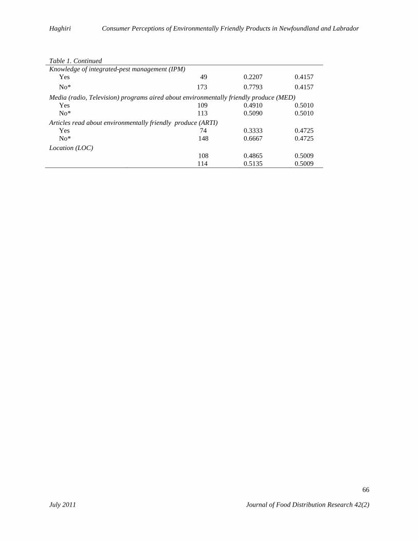
Haghiri Consumer Perceptions of Environmentally Friendly Products in Newfoundland and Labrador
66 July 2011 Journal of Food Distribution Research 42(2)
Table 1. Continued Knowledge of integrated-pest management (IPM)
Yes 49 0.2207 0.4157 No* 173 0.7793 0.4157
Media (radio, Television) programs aired about environmentally friendly produce (MED) Yes 109 0.4910 0.5010 No* 113 0.5090 0.5010
Articles read about environmentally friendly produce (ARTI) Yes 74 0.3333 0.4725 No* 148 0.6667 0.4725
Location (LOC) 108 0.4865 0.5009 114 0.5135 0.5009

67
Repeat Buying Behavior for Ornamental Plants: A Consumer Profile Marco A. Palma, Charles R. Hall and Alba Collart This paper used an electronic survey conducted in Texas to study the main factors affecting the frequency of pur-chase, measured in transactions per month, for ornamental plants. While we found several differences in demo-graphic characteristics of respondents, the two major factors impacting the frequency of buying for ornamental plants were the purpose of the purchase (self use vs. gifts) and seasonality. Respondents with a college degree in the older age groups, and higher income levels had a lower frequency of buying while individuals with medium income levels increase frequency of buying. Several ornamental plant attributes were also included in the analysis. The floriculture and nursery industry has evolved rapidly in recent years. The introduction of mass-market retailers such as supermarkets, department stores and Internet-based businesses has changed the marketing paradigm of floricul-ture and nursery products. Floriculture and Nursery crops, often referred to as the green in-dustry are an important sector of the U.S. agri-cultural economy with grower cash receipts of $16.9 billion in 2006 (Jerardo, 2007). All green industry sectors, including growers, landscaping design and maintenance, and retail, are estimat-ed to contribute over $148 billion in economic impacts to the U.S. economy and add almost 2 million jobs (Hall et al., 2006).
In general, the demand for all products is highly dependent on its characteristics or attrib-utes, which include satisfying nutritional needs and/or taste (Hanemann, 1984). Even though ornamental plants do not satisfy any nutritional needs, they possess other important attributes that influence the buying decision including their aesthetic value; In addition to ornamental attributes, consumer demand for ornamental products is also affected by consumer de-mographics and the buying occasions and peri-ods (Palma and Ward, 2010). Understanding how consumers make choices of whether to buy ornamental products or not, and the intensity and frequency of purchase is essential to understand-ing ornamental demand. Floriculture and nursery
Palma is an Assistant Professor and Extension Economist in the Department of Agricultural Economics at Texas A&M University. Hall is a Professor in the Department of Horticultural Sciences and Holder of the Ellison Chair of International Floriculture at Texas A&M. Collart is a Grad-uate Assistant in the Department of Agricultural Economics at Texas A&M University.
products are purchased for various reasons such as expression of love or friendship, a way to ex-press thankfulness or appreciation, and beautifi-cation purposes either for self use or as gifts. Plant and flower attributes are not easily quanti-fied and very subjective; therefore the satisfac-tion (utility) gained from the consumption of ornamental products can be influenced by the characteristics or preferences of buyers (de-mographics) and the reasons for buying the products (Girapunthong, 2002). This situation becomes evident during special seasonal buying occasions (i.e., Mother’s Day, Valentine’s Day, etc), where the consumption of ornamental products is substantially higher compared to non-calendar occasions.
The main objective of this paper is to analyze the effects of product attributes, consumer char-acteristics (demographics) and seasonal factors affecting consumer demand for ornamental plants. Specifically, we will look at the frequen-cy of buying, measured in transactions per month as a function of ornamental plant fea-tures, socio-economic characteristics, and con-sumer habits (including seasonality). Frequency of purchasing multiplied by expenditures per transaction yields total sales for the ornamental plant industry. Understanding what factors in-fluence buyers to increase frequency of purchas-ing is essential for ornamental plant grower’s profitability.
There is extensive literature regarding de-mand analysis for traditional agricultural prod-ucts, such as milk (Gould et al., 1990), meat (Glynn et al., 2010), fruit and vegetables (Rick-ard et al., 2009), etc.; however, studies on the demand side for floriculture and nursery prod-ucts are very limited in the literature, with the

Palma et al. Repeat Buying Behavior for Ornamental Plants: A Consumer Profile
68 July 2011 Journal of Food Distribution Research 42(2)
majority of consumer demand and preferences studies focusing in floricultural crops. Miller (1983) performed an extensive sub-sector analy-sis for the fresh cut-flower industry in the U.S. by analyzing the structure, conduct and perfor-mance of the existing conditions of the industry in an attempt to predict future trends. Miller ob-served that there were special calendar occasions when the demand for flowers was substantially higher and other non-calendar occasions where the demand was substantially lower. He also determined that the demand for flower arrange-ments was inelastic, meaning that consumers are not highly responsive to changes in price of flo-ral products.
Tilburg (1984) analyzed a panel of cut flower and potted plant consumers in the Netherlands to relate aspects of consumer behavior to market-ing variables and demographic characteristics of households. He identified three market seg-ments: the first segment consisted of 44 percent of the households and was sensitive to prices but insensitive to national advertisements; the se-cond segment consisted of 40 percent of the households, and was insensitive to both prices and advertisements; and the third segment, with 13 percent, was sensitive to both prices and ad-vertising.
Behe (1989) analyzed consumer floral pur-chasing behavior of Pennsylvanians at the retail level. She recommended three ways to segment retail flower markets: by product, volume of purchase, and by location of the purchase. Behe et al. (1992a) carried out an analysis of consum-er purchases of floral products in Ohio super-markets using principal components analysis that yielded 34 independent factors accounting for 64% of the total variance affecting floral purchases. These factors were grouped into five main categories, including, product, consumer, store, use (gift), and location. Behe et al. (1992b) followed up on her previous study and applied cluster analysis to identify the most im-portant factors affecting floral buying decisions by market segments. She used demographic characteristics and purchase factors identified in her previous work to profile market segments and distinguishing elements. Becker (1993) studied differences in service quality between supermarkets and florists in Texas. He found
that the differences on the types of retail outlets were based on the types of products sold, custom design and other in-store services, delivery op-tions and convenience. Rimal (1998) analyzed the effects of generic and brand promotions on sales of fresh cut-flowers at the retail level in the U.S.
Girapunthong (2002) analyzed the demand drivers for fresh cut-flowers and their substitutes in the U.S. Girapunthong found that all direct price effect coefficients with the seasonal and actual variables were statistically significant and changes in the relative prices had a significant impact on flower market shares among fresh cut-flowers, potted flowering plants, and dry/artificial flowers. Ward (2004) evaluated the impacts of the Flower Promotion Organization (FPO) advertising campaign on cut-flower sales, concluding that the promotions have impacted the demand for flowers through increasing buyer frequency and through attracting new buyers. He found that about 87 percent of the increase in demand for the promotional programs is from the increased number of transactions per buyer. Ward found that the demographic group that responded the most to the promotional program were female buyers that purchase flowers for self-use. This was consistent with the target of the FPO promotion program. Yue and Behe (2008) analyzed consumer preferences for dif-ferent floral retail outlets. They used a consumer panel data collected by the American Floral En-dowment from 1992 to 2005 were used to evalu-ate consumers' choice of different floral retail outlets among box stores, traditional freestand-ing floral outlets, general retailer, other stores, and direct-to-consumer channels. Palma and Ward (2010) estimated ornamental demand for four different ornamental products, including cut flowers, plants, dry/artificial and outdoor. They divided demand into two components, market penetration and buying frequency. They con-cluded that demand drivers for ornamental con-sumption was driven by the entry of new buyers rather than repeat buying customers increasing their number of transactions.
When studying the aforementioned literature regarding the demand for floral and nursery products, it is apparent that there are many fac-tors that affect their demand. These factors can

Palma et al. Repeat Buying Behavior for Ornamental Plants: A Consumer Profile
69 July 2011 Journal of Food Distribution Research 42(2)
be grouped into three main categories: external, controlled, and seasonal factors. External or macro-factors of demand are those affecting in-dustry businesses but for which firms have no mechanism to change their output. These include inflation, wages, prices, unemployment rate, demographic factors and other macro-economic variables. Controlled factors of demand are those factors that may be used to influence per-ceptions and awareness with the use of promo-tions, product development and innovations. Seasonal factors are also important for floral and ornamental plants because of the nature of the products and the reasons for buying (Ward, 1997).
Because ornamental plants are not satisfying nutritional needs like most food products, in a typical month the percentage of the population that buys flowers and ornamental plants is rela-tively low. Hence, it is important to understand how ornamental plant buyers make the choice to purchase and to have a measure or profile of consumer purchase intensity. Demand analyses for ornamental products differ among other agri-cultural commodities in the sense that for other agricultural commodities, the quantity consumed is used directly in the analysis. In the case of floriculture products, a consumer purchase quan-tity is ambiguous and closely tied to the type of ornamental plant; for example, a quantity of one may refer to one single stem rose, or an ar-rangement of a dozen roses and several other plants. Hence, this study replaces quantity (number of units) observed by the number of transactions given on a defined period of time. In doing so, all properties (or restrictions) of the demand function are still satisfied.
Repeat buying occurs when a consumer buys a product more than once in a given period of time. Consumers are influenced by pre-purchase needs, perspectives, attitudes, the experience of previous usage, and external influences such as advertising and promotion programs, retail availability, personal selling and word of mouth effects, and differences in products, services and prices. The consumer has to make decisions re-garding what products to buy and at what prices and where to buy the products. All of these characteristics form a post-buying experience in the customer’s mind after the purchase takes
place; based on all these factors a consumer would choose depending on the level of satisfac-tion or utility obtained from the product or ser-vice whether to re-purchase the product or not.
There are basically three cases of repeat buy-ing situations that can be defined. First, if a con-sumer buys more than one product in one or more purchase occasions (transactions) in a giv-en time period. In this case, consumers differ in how often they repeat buy the products. The fre-quency of buying would be 0 for a consumer that did not purchase the product and 1 for con-sumers that purchased the product once. For re-peat buyers, the frequency will be 2, 3, 4, etc., depending on the number of repeat buying occa-sions they purchased the product. The second way of repeat buying refers to consumer that may buy the product in more than one time peri-od, or multiple transactions in a given period. Then a model can be formulated for repeat buy-ing behavior under stationary and no trend con-ditions. The third and last form of repeat buying behavior is that more than one unit may be pur-chased on the same purchase occasion (Ehren-berg, 1988).
Data and Methods The conceptual framework for this study is based in the random utility theory. A random utility model assumes that the utility function for a consumer has two components, one that is de-terministic, and one that is not observable and therefore treated as random variables (Carpio et al., 2008). The unobservable portion treated as random variables could be characteristics of the consumers or the products. Following Hane-mann (1984), the utility obtained from consum-ing ornamental plants can be written as:
where x represents a vector of ornamental plant commodities, z is all other commodities, b represents ornamental plant features (attributes), s represents consumer socio-demographic char-acteristics, and ε is a random vector of unob-servable consumer or ornamental plant charac-teristics. The consumer chooses (x,z) to maxim-ize utility subject to a budget constraint:
(1) ),,,,( εszbxu

Palma et al. Repeat Buying Behavior for Ornamental Plants: A Consumer Profile
70 July 2011 Journal of Food Distribution Research 42(2)
And the non-negativity constraints:
The data were obtained through an electronic mail survey conducted in July of 2008 to a rep-resentative sample of the Texas population fol-lowing Dillman’s tailored design method (Dill-man, 2007). The survey sample consisting of 880 individuals provided by MarketTools Cor-poration, a company specialized in market re-search and online survey services. From the total sample, approximately 31% were actual consumers of the ornamental industry’s prod-ucts, lowering the final number of usable re-sponses to 274 observations.
The dependent variable is frequency of buy-ing for ornamental plants. It is defined as the number of transactions per month ( nfi ,...,3,2,1,0= ) and it is a function of the purpose of the purchase (PP), seasonality (S), price (P), ornamental plant features including low care demanding (LCD), organically grown (ORGANIC), light demanding (LD) Guaranteed growth (GG), drought tolerant (DT), vibrant colors (VC), and several demographic character-istics, including age, gender, marital status, in-come, ethnicity, education, and region. The pur-pose of the purchase is to use the ornamental plants for self consumption or gifts. The fre-quency of buying of flowers is affected by sea-sonal factors. As an example, the frequency of buying and the total number of buyers increase during special calendar occasions such as Moth-er’s Day, Valentine’s Day, Christmas, etc. Since our data are not time series, monthly seasonality cannot be evaluated. The variable seasonality is a discrete variable that identifies self described special occasion buyers only (non-habitual buy-ers), versus habitual ornamental buyers. There is also a random term ε that represents unobserved consumer or ornamental plant features. The de-pendent variable frequency of buying is cen-sored and therefore the Tobit model is used for the estimation. The general frequency of buying econometric model can be written as:
(4)
i
i
SPPREGREGEDUEDUETETINCINCINCMARRIEDFEMALEAGE
AGEAGEPCOLORDTGGLDORGANICLCDf
εββββββββββββββ
ββββββββββ
++++++++++++++
++++++++++=
2322212019
1817161514
13121110
98765
43210
3232324324
32
where all variables used in the model and
their definition are presented in Table 1 (see Appendix).
Because the dependent variable in our regres-sion model equation has a lower limit (i.e. zero), and the dependent variable takes the value of zero for a large number of sample observations (24.8%), conventional multiple regression anal-ysis is not an appropriate technique to be used (Lung-Fei and Maddala, 1985). In order to ac-count for this truncation on the data set the Tobit model can be specified as follows (Greene, 2000):
where ix′ is the (1 × K) vector of explanatory
variables and ),0(~ 2σε Ni and it is independ-ent of other errors. Thus for any household the buying frequency model would take the form:
From the total number of observations N in
the sample, the number of observations can be divided into two groups; one for which 0=if ,
0N ; and another for the number of observations for which 0>if , 1N . In order to observe the statistical problems arising from the censored sample problem, consider leaving out of the analysis the 0N observations for which 0=if . For the remaining 1N sample observations, they are complete observations. Hence, one can use least squares estimators to estimateβ . The prob-lem is that this estimator is biased and incon-sistent. In order to prove that, one can write
(2) ∑ =+ yzxp jj
(3) 0,0 ≥≥ zx j
(5) iii xf εβ +′=* ,
(6) *ii ff = if 0* >if
0=if if 0* ≤if .

Palma et al. Repeat Buying Behavior for Ornamental Plants: A Consumer Profile
71 July 2011 Journal of Food Distribution Research 42(2)
down the expectation of the observed values of if conditional on the fact that 0>if :
(7).. [ ] ( )0|0| >+′=> iiiii fExffE εβ
If the conditional expectation of the error term is zero, then the estimates of the least square regression on 1N would provide an unbi-ased estimator for β . However this is not the case; if the iε are independent and normally distributed random variables, then the expecta-tion would be:
(8) [ ] [ ] 0|0| >′−>=> βεεε iiiii xEfE
It can be shown that this conditional expecta-tion can also be expressed in the following man-ner:
(9) [ ]i
iiii xE Φ=′−> φσβεε |
where iφ and iΦ are the standard normal
probability distribution function (p.d.f), and cu-mulative distribution function (c.d.f.) evaluated at )/( σβix′ ; therefore in the regression model, if 0>if , then,
(10)
if we apply the regular least squares procedures the term
i
i
Φφ
σ is omitted. Since that term is not
independent of ix the results are biased and in-consistent.
The parameters were estimated with Time Series Processor (TSP) version 4.5 (Hall, 1992). The estimation procedure uses the analytic first and second derivatives to obtain maximum like-lihood estimates via the Newton-Raphson algo-rithm. The starting values for the parameters are obtained from a regression on the observations with positive f values. The numerical implemen-tation involves evaluating the normal density and cumulative normal distribution functions.
The cumulative distribution function is comput-ed from an asymptotic expansion, since it has no closed form. The ratio of the density to the dis-tribution function, used in the derivatives, is also known as the Inverse Mills Ratio. Results and Discussion As shown in Table 2 (see Appendix), the survey sample was a fair representation of the Texas’ population based on selected socio-demographic characteristics including marital status, gender, ethnicity, and income. About 60% of respond-ents were married compared with 54% of the population in Texas. The percentage of females in the sample was 53% versus 50% for Texas; and 53% of the total number of respondents had an income of more than $50,000 compared to 47% of Texas’ population. The ethnical distribu-tion of the sample was similar to the U.S. Cen-sus Bureau data, with Caucasians accounting for the majority of responses in the survey and comprising the majority of the true population, followed by Hispanics. The highest educational degree obtained from 78% of the sample popula-tion was a bachelor’s degree compared with 92% of Texas’ population.
Most respondents (78.5%) reported to be non-habitual ornamental buyers or purchasers of ornamental plants during special calendar buy-ing occasions only. Most (84%) ornamental products in Texas were purchased for self-consumption purposes. The preferred outlets to purchase ornamental products were garden cen-ters (72%), followed by nurseries (40%), chain stores (32%), and supermarkets (30%).
Respondents were also asked to rate, from 1-5, the importance of several aspects in the pur-chase decision including price (3.89), vibrant colors (3.85), low-care demand (3.83), drought tolerance (3.64), season (3.57), guaranteed growth (3.51), light demand or requirement (3.34), and organic (2.58). The weighted average rating of these aspects clearly suggests that price is the most important feature, followed very closely by vibrant colors and low-care demand (low maintenance). The rating of organically-grown and light requirement implies that these two features are typically not very important to Texas consumers when making purchasing deci-
ii
ii
iii
ux
xf
+Φ
+′=
+′=φσβ
εβ

Palma et al. Repeat Buying Behavior for Ornamental Plants: A Consumer Profile
72 July 2011 Journal of Food Distribution Research 42(2)
sions for ornamental plants. For instance, 45% of the respondents assigned low ratings of 1 or 2 to organically-grown products and 36% con-firmed that light requirement was not a feature they carefully seek for when buying an orna-mental plant.
The parameter estimates of the buying fre-quency model for ornamentals are presented in Table 3 (see Appendix). The strong significance of the sigma parameter suggests that for the data truncation, the lower limit level of zero can not be ignored and the estimation method must deal with the asymptotic distribution of the data. This parameter refers to the estimated standard devia-tion of the residual. In this model, 184 out of 249, or 73.9% of the usable observations were positive. The frequency of buying for the aver-age respondent was 1.36 transactions per month. The sign of the parameters can be interpreted as an increase (positive), or decrease (negative) in the monthly frequency of buying measured in number of transactions per month. The marginal effects represent the change in the monthly fre-quency of buying for an additional unit of the variable. Since most of the variables in the mod-el are dummy variables, then marginal effects are interpreted as the change in the number of transactions per month associated to that dummy variable. For example, low care demanding plants (LCD) would increase the monthly fre-quency of purchasing by 0.0256. On the contra-ry, if a plant is not low care demanding, then the monthly frequency of purchase would be re-duced by 0.0256 transactions
The price coefficient is, as expected, nega-tive, in accordance to economic theory (Nichol-son, 1998). There was no statistical significant influence associated with younger age groups and frequency of buying. Age2 (25-39 years old), Age3 (40-55 years old) and Age4 (more than 55 years old) all decreased frequency of buying. For individuals of 25-39 years of age, frequency of buying was reduced by 0.03 trans-actions per month, while 40-55 years of age had 0.08 less transactions per month, and individuals older than 55 had 0.05 less transactions per month. Respondents with incomes between $25,000 and $49,999 had a higher frequency of buying, with 0.06 more transactions per month. No other income groups had statistically signifi-
cant effects on frequency of buying. Higher in-come groups (Inc3 and Inc4) had negative mar-ginal effects of about 0.02 less transactions per month. Ethnicity was not found to have statisti-cally significant effects on buying frequency. Individuals with a college degree tend to make 0.08 less transactions per month. The two varia-bles with the highest effects on frequency of purchasing were purpose of the purchase (PP) and seasonality (S), with both variables increas-ing the frequency of buying. When the purpose of the purchase was for self-use, the model showed an increase in the number of transaction per month of 0.09. The seasonality variable sought to differentiate between those individuals making most of their ornamental purchases dur-ing special calendar occasions, such as Valen-tine’s Day, Mother’s Day and Christmas, etc. and those individuals who also purchase orna-mentals in non-calendar occasions (year-round). Respondents who purchase ornamentals year-rounded increase frequency of buying by 0.2165 transactions per month. No statistically signifi-cant differences in frequency of buying were found among Texas regions.
Summary and Conclusions This paper used an electronic survey conducted in Texas to study the main factors affecting the frequency of purchase, measured in transactions per month, for ornamental plants. The frequency of buying for the average buyer was 1.36 trans-actions per month. Major factors affecting con-sumer frequency of purchase in transactions per month were grouped into ornamental plant fea-tures, socio-demographic characteristics (includ-ing regional differences), and consumer habits. While several differences in demographic char-acteristics of respondents and ornamental plant features were found, consumer habit factors im-pacted the frequency of ornamental plants buy-ing the most, including the purpose of the pur-chase and seasonality. The marginal effects for each variable shown in Table 3 show the in-crease/decrease in the number of transactions per month if everything else is held constant. When the purpose of the purchase was to use ornamental plants for self-consumption the fre-quency of transactions per month increased 0.09

Palma et al. Repeat Buying Behavior for Ornamental Plants: A Consumer Profile
73 July 2011 Journal of Food Distribution Research 42(2)
or 6.9%. Those respondents who were self-described as habitual buyers (bought products during non-special seasonal occasions) increased the number of transactions per month by 0.21 or 15.9%. In terms of ornamental plant features, light demanding plants and purchase price had a negative effect in frequency of purchase. Light demanding plants reduce consumer frequency of purchase 0.04 per month (3.0%). Drought toler-ant plants had a positive effect in frequency of purchasing by increasing it 0.03 (2.8%). There were also socio-demographic factors that influ-enced consumer frequency of purchasing. Older age groups (Age3: 40-55 years, and Age4: 55 or older) and respondents with a college degree had a lower frequency of buying. Individuals with medium income levels ($25,000 to $49,999) in-crease frequency of buying by 0.06 transactions per month (4.5%). No statistically significant effects of ethnicity or regional differences in the state of Texas were found on frequency of buy-ing.
While there may have been some product or consumer features not included in the specifica-tion of our econometric model, these results provide useful insights for ornamental plant growers in terms of the factors affecting fre-quency of purchase for ornamental plants. Fre-quency of purchase measured in number of transactions per month multiplied by expendi-tures per transaction yield total sales. Under-standing which ornamental plant features affect the number of transactions during non-special seasonal occasions is vital information for grow-ers. Socio-demographic characteristics of orna-mental plant consumers and their effect in fre-quency of buying can be used to target specific groups for promotions. References
Becker, W.A. 1993. “Products, Services, and
Consumer Perceptions of Service Quality in the Retail Floral Industry of Texas.” PhD Dissertation. Texas A&M University. Col-lege Station, Texas.
Behe, B.K. 1989. “Floral Purchase Behavior of Pennsylvanians.” PhD Dissertation. Penn-sylvania State University. University Park, Pennsylvania.
Behe, B.K., T.A. Prince, and H.K. Tayama. 1992a. “Analysis of Consumer Purchases of Floral Products in Supermarkets.” Hortscience. Vol. 27:455-459.
Behe, B.K., T.A. Prince, and H.K. Tayama. 1992b. “Market Segmentation of Supermar-ket Floral Customers.” Hortscience. Vol. 27:455-459.
Carpio, C.E., M.K. Wohlgenant, and C.D. Safley. 2008. “Relative Importance of Fac-tors Affecting Customer’s Decisions to Buy Pick-Your-Own Versus Preharvested Fruit at North Carolina Farms” Journal of Agricul-tural and Applied Economics. Vol. 40. No. 3: 983-997.
Dillman, D. A. 2007. Mail and Internet Surveys: The Tailored Design Method. Second Edi-tion. John Wiley and Sons, Inc. New Jersey, New Jersey.
Ehrenberg, A.S. 1988. Repeat-Buying, Facts, Theory and Applications. Oxford University Press. New York, New York.
Girapunthong, N. 2002. “Demand Drivers for Fresh Cut Flowers and Their Substitutes: An Application of Household Expenditure Allo-cation Models.” Ph.D. Dissertation. Food and Resource Economics Department. Uni-versity of Florida. Gainesville, Florida
Glynn, T.T., J.R. Mintert, and T.C. Schroeder. 2010. “U.S. Meat Demand: Household Dy-namics and Media Information Impacts” Journal of Agricultural and Resource Eco-nomics. Vol. 35. No. 1:1-17.
Greene, W.H. 2000. Econometric Analysis. 4th Edition. Prentice Hall. Upper Saddle River, New Jersey.
Gould, B.W., T.L. Cox, and F. Perali. 1990. “The Demand for Fluid Milk Products in the U.S.: A Demand Systems Approach” West-ern Journal of Agricultural Economics. Vol. 15. No. 1:1-12.
Hall, B.H. 1992. Time Series Processor Ver-sion 4.5. Reference Manual. Palo Alto, Cal-ifornia.
Hall, C.R., A.W. Hodges, and J.J. Haydu. 2006. “The Economic Impacts of the Green Indus-try in the U.S.”HortTechnology. Vol. 16:345–353.

Palma et al. Repeat Buying Behavior for Ornamental Plants: A Consumer Profile
74 July 2011 Journal of Food Distribution Research 42(2)
Hanemann, W.M. 1984. “Discrete/Continuous Models of Consumer Demand” Econometri-ca. Vol. 52. No. 3: 541-562.
Jerardo, A. 2007. “Floriculture and Nursery Crops Yearbook.” Economic Research Ser-vice, U.S. Department of Agriculture, Sep-tember 2007. Washington, DC.
Lung-Fei, L. and Maddala, G.S. 1985. “The Common Structure of Tests for Selectivity Bias, Serial Correlation, Heteroscedaticity, and Non-normality in the Tobit Model.” In-ternational Economic Review. Vol. 26. No. 1: 1-20.
Miller, M. 1983. “Commodity Sub-Sector Anal-ysis of Cut Flower Industry.” PhD. Disserta-tion. Food and Resource Economics Depart-ment. University of Florida. Gainesville, Florida.
Nicholson, W.1998.Microeconomic Theory: Basic Principles and Extensions. Dryden Press. Fort Worth, Texas.
Palma, M.A. and R.W. Ward. 2010. “Measuring Demand Factors Influencing Market Penetra-tion and Buying Frequency for Flowers in the U.S.” International Food and Agribusiness Management Review. Vol. 13. No. 1: 65-82.
Rickard, B.J., C.M. Pierre, and G.M. Becker. 2009, “Drivers of Demand for Imported Ag-ricultural Commodities: A Cross-Country Comparison” International Food and Agri-business Management Review. Vol. 12. No. 2: 19-38.
Rimal, A.P. 1998. “Effect of Generic and Brand Promotions of Fresh Cut Flowers on the Use of Retail Flower Outlets.” Ph.D. Disserta-tion. Food And Resource Economics. Uni-versity of Florida. Gainesville, Florida.
Tilburg, A.V. 1984. “Consumer Choice of Cut Flowers and Pot Plants.” Agricultural Uni-versity. Wageningen, The Netherlands. No. 84-2
Ward, R.W. 1997. “Evaluating Promoflor: Have the Promotions of Fresh Cut Flowers and Greens Had an Impact.” National Promoflor Council. UF/PER97#2. University of Flori-da. Gainesville, Florida.
Ward, R.W. 2004. “Estimated the Impact of FPO’s Generic Promotions of Fresh Cut Flowers: Analysis Through Phase VI.” Re-search Paper. Food And Resource Econom-ics. University of Florida. Gainesville, Flor-ida.
Yue, C. and B.K. Behe. 2008. “Estimating U.S. Consumer’s Choice of Floral Retail Outlets.” Hortscience. Vol. 43. No. 3:764-769.

Palma et al. Repeat Buying Behavior for Ornamental Plants: A Consumer Profile
75 July 2011 Journal of Food Distribution Research 42(2)
Appendix Table 1. Description of Variables Included in the Ornamental Plant Buying Frequency Model. Variable Description Ornamental plant features
LCD Low care demanding ORGANIC Organically grown LD Light demanding GG Guaranteed growth DT Drought tolerant COLOR Vibrant colors P Price Socio-demographic characteristics
AGE2 Age between 25-39 years old (= 1 if true and 0 otherwise) AGE3 Age between 40-55 years old (= 1 if true and 0 otherwise) AGE4 More than 55 years old (= 1 if true and 0 otherwise) FEMALE If gender is a female (= 1 if true and 0 otherwise) MARRIED Married marital status (= 1 if true and 0 otherwise) INC2 Income level (= 1 if income between $25,000- $49,999 and 0 otherwise) INC3 Income level (=1 if income between $50,000-$74,999 and 0 otherwise) INC4 Income level (=1 if income is $75,000 or more, and 0 otherwise ET2 Ethnicity (=1 if ethnicity is Hispanic, and 0 otherwise) ET3 Ethnicity (=1 if ethnicity is other, and 0 otherwise) EDU2 Education level (=1 if college degree, and 0 otherwise) EDU3 Education level (=1 if graduate school, and 0 otherwise) Consumer habits S Seasonality (= 1 if habitual buyers – non special occasion only- and 0 otherwise) PP Purpose of the purchase (= 1 if self consumption and 0 otherwise) Region DREG2 Region: Central Texas (= 1 if true and 0 otherwise) DREG3 Region: South Texas (= 1 if true and 0 otherwise)
Dummy variables base levels AGE1 Age group of under 25 years INC1 Income group of under $25,000 ET1 Ethnicity is Caucasian EDU1 Education level is high school or less REG1 Region is north

Palma et al. Repeat Buying Behavior for Ornamental Plants: A Consumer Profile
76 July 2011 Journal of Food Distribution Research 42(2)
Table 2. Representativeness of the Survey Respondents Relative to the Texas Census Population Data. Survey Data Census Data
Demographic variables Frequency Percentage Percentage
Marital status Married 163 59.9 53.5 Single 109 40.1 46.5 Gender Male 129 47.3 49.8 Female 144 52.7 50.2 Education level High School 32 11.8 48.4 College 181 66.5 43.5 Graduate School 59 21.7 8.1 Ethnicity African American 10 3.7 11.5 Caucasian 210 76.9 47.0 American Indian 6 2.2 0.7 Hispanic 29 10.6 36.0 Asian/Pacific Islander 12 4.4 3.4 Other 6 2.2 1.3 Age Less than 25 35 12.9 38.7 25-39 69 25.5 15.2 40-55 81 29.9 28.4 More than 55 86 31.7 17.6 Income Under $25,000 45 16.4 26.7 $25,000-$50,000 85 31.0 26.6 $50,001-$75,000 57 20.8 17.9 $75,001-$99,999 36 13.1 11.3 $100,000-& above 51 18.6 17.5
Source: U.S. Census Bureau, 2000 and 2005-2007 American Community Survey

Palma et al. Repeat Buying Behavior for Ornamental Plants: A Consumer Profile
77 July 2011 Journal of Food Distribution Research 42(2)
Table 3. Results from a Tobit Model Analyzing the Frequency of Buying Ornamental Plants. Tobit
Variable Coefficient
Standard
Error t-value
Marginal
Effects Intercept 0.5946 0.8983 0.6620 0.0904 Ornamental plant features
LCD 0.1687 0.1568 1.0755 0.0256 ORGANIC 0.1781 0.1196 1.4890 0.0271 LD -0.2686*** 0.1580 -1.7004 -0.0408 GG 0.1709 0.1527 1.1189 0.0260 DT 0.2542*** 0.1496 1.6995 0.0386 COLOR -0.0660 0.1540 -0.4283 -0.0100 P -0.2974** 0.1469 -2.0245 -0.0452 Socio-demographic characteristics
AGE2 -0.1984 0.2309 -0.8592 -0.0301 AGE3 -0.5265** 0.2115 -2.4895 -0.0800 AGE4 -0.3173 0.2176 -1.4582 -0.0482 FEMALE 0.0800 0.2593 0.3084 0.0122 MARRIED 0.2223 0.2749 0.8086 0.0338 INC2 0.4008*** 0.2088 1.9199 0.0609 INC3 -0.1176 0.2360 -0.4981 -0.0179 INC4 -0.1038 0.2325 -0.4467 -0.0158 ET2 -0.0734 0.3161 -0.2321 -0.0115 ET3 0.0782 0.2867 0.2729 0.0119 EDU2 -0.5342* 0.1837 -2.9076 -0.0812 EDU3 0.3178 0.2344 1.3560 0.0483 Consumer habits PP 0.6183*** 0.3491 1.7709 0.0940 S 1.4246* 0.3164 4.5030 0.2165 Region REG2 -0.1542 0.1753 -0.8795 -0.0234 REG3 0.2994 0.2463 1.2157 0.0455 SIGMA 1.8173* 0.1002 18.1449
Number of usable observations 249 * P-value ≤ 0.1, ** P-value ≤ 0.05, *** P-value ≤ 0.01

78
Does the WTO Increase Trade? The Case of U.S. Cocoa Imports from WTO-Member Producing Countries Osei-Agyeman Yeboah, Saleem Shaik, Shawn J. Wozniak and Albert J. Allen This study analyzes U.S. cocoa bean imports from twenty-one major cocoa-producing and exporting countries dur-ing the pre- and post-liberalization period of 1970-2008 using the gravity equation and a linear one-way fixed effects model. The objective was to measure trade creation for a World Trade Organization (WTO) member that has under-gone trade liberalization. Cocoa beans can serve as a proxy for any tropical commodity upon which a developing country heavily relies on for export revenue, such as is the case with cocoa for Côte d’Ivoire and Ghana, for exam-ple. Our results find participation in free trade agreements (FTAs) and WTO membership do contribute to increased U.S. cocoa bean imports at the one percent and five percent confidence levels, respectively. U.S. imports of cocoa beans have grown in re-cent years. This is due to increased cocoa pro-duction, lower world prices, greater centraliza-tion and efficiency in the supply chain, greater consumer demand for chocolate products due to the introduction of various niche markets, in-creased consumer per capita income, and trade liberalization, among other causes. Market ac-cess to export cocoa beans in many cocoa pro-ducing countries has improved greatly due to trade liberalization in the cocoa sector. This has been accomplished through a variety of policy instruments, primarily structural adjustment pro-grams (SAPs).
In reducing or eliminating the role of state-owned and operated marketing and exporting boards, cocoa-producing countries have opened themselves up to foreign-owned corporate agri-business exporting companies and producers have received a higher share of a lower world price. U.S. and European transnational corpora-tions have become increasingly involved in more aspects of the cocoa bean supply chain, Yeboah is Associate Professor and Interim Director, L. C. Cooper, Jr. International Trade Center, North Carolina A&T State University. Shaik is Assistant Professor, De-partment of Agribusiness and Applied Economics, North Dakota State University. Wozniak is Agricultural Econo-mist for Economic Research Service, United States De-partment of Agriculture. Allen is Professor, Department of Agricultural Economics, Mississippi State University.
The views expressed here are those of the authors, and may not be attributed to the Economic Research Service or the U.S. Department of Agriculture.
The authors wish to thank two anonymous reviewers and the Editor Dovi Alipoe for comments and suggestions on an earlier version of this article. Any remaining errors or omissions are those of the authors.
becoming the buyers and exporters of cocoa beans in producing countries with the scaling back or dissolution of commodity marketing boards in those countries. These corporations have also centralized grindings from a number of companies into the control of a few, larger corporations and have increased grindings in the producing countries.
Trade liberalization was also accomplished through free trade agreements (FTAs) in a few countries from which the United States imports fewer cocoa beans than those that underwent SAPs. Free trade agreements are those in which a designated group of countries have agreed to reduce or eliminate tariffs, quotas and trade preferences on many or most goods and services traded between them. This study also discusses the role that the World Trade Organization (WTO) has in agricultural negotiations. The World Trade Organization is an intergovernmen-tal body regulating tariffs and trade. This section presents an overview of trade liberalization in the cocoa industry, changes in the market struc-ture of exporting and marketing companies, and the U.S. market for cocoa beans and products.
Prior to trade liberalization, cocoa trade was inefficient and the share of the f.o.b. price re-ceived by farmers was small (Varangis & Schreiber, 2001). Marketing boards were largely responsible for these faults, taking the lion’s share of the f.o.b. in taxes while returning only some of it in the form of extension services and seed varieties. Many farmers smuggled cocoa to neighboring countries when those countries’ market price was higher than their own, inflating export figures for the higher-priced countries and deflating prices for lower-priced countries

Yeboah et al. Does the WTO Increase Trade? The Case of U.S. Cocoa Imports from WTO-Member Producing Countries
79 July 2011 Journal of Food Distribution Research 42(2)
(Bulíř, 2003). Cocoa exports were on the decline in many countries, such as Nigeria, where ex-ports in 1985 – after the implementation of SAPs – were still below their 1970 levels, as oil became more vital to that country’s economy (Kwanashie, Ajilima & Garba, 1998).
Following historically low prices in the 1970s, many cocoa producing countries under-went trade liberalization under SAPs from the World Bank and International Monetary Fund (IMF). In Nigeria, SAPs were used as the “only alternative” toward improving agricultural out-put (Kwanashie, Ajilima & Garba, 1998). Mar-keting boards were restructured, replaced or eliminated and opened up to competition from private marketing and export companies. Begin-ning in the 1980s, these processes are still un-derway in Ghana and Côte d’Ivoire, the two highest-volume cocoa-producing countries in the world.
Trade liberalization has had both positive and negative impacts. It has brought a greater share
of the f.o.b. price to cocoa bean farmers (Varan-gis & Schreiber, 2001). This greater share, though, is of a lower world price as production has grown and prices have harmonized across borders (Figure 3, Gilbert & Varangis, 2003). Marketing boards’ roles have been reduced or eliminated and transnational corporations have replaced them in buying and exporting cocoa beans (Fold, 2002). Exporting has also under-gone centralization, as these transnational firms have exercised comparative advantage against smaller firms (Fold, 2001). But by opening up markets to foreign competition, farmers have become more vulnerable to price fluctuations, great and small, on the world market. World prices have also converged between countries and fallen during the trade liberalization period (Figure 1). For U.S. imports, trade liberalization has signaled lower world prices for firms buying cocoa beans from producing countries and lower prices for U.S. consumers buying the cocoa and chocolate products derived from them.
Figure 1. Deflated Cocoa Producer Prices and Deflated ICCO Indicator Price, West African Countries (1985 = 100)

Yeboah et al. Does the WTO Increase Trade? The Case of U.S. Cocoa Imports from WTO-Member Producing Countries
80 July 2011 Journal of Food Distribution Research 42(2)
The move under trade liberalization from protectionist agricultural commodity policies toward open market policies for cocoa beans has implications for other commodities, as well, such as coffee, tea, sugar and cotton. These is-sues are especially relevant during the current Doha Round of WTO negotiations, which are at an impasse as developing countries whose econ-omies are dependent on agriculture square off against industrial countries seeking the develop-ing countries’ full market liberalization for agri-cultural goods.
This study researches the effects of trade lib-eralization and U.S. cocoa bean imports from twenty-one cocoa-producing and exporting countries for the pre- and post-liberalization pe-riod of 1970-2008. These countries are Brazil, Cameroon, Colombia, Costa Rica, Côte d'Ivoire, Dominican Republic, Ecuador, El Salvador, Ghana, Guatemala, Haiti, Honduras, Indonesia, Malaysia, Mexico, Nicaragua, Nigeria, Panama, Papua New Guinea, Trinidad and Tobago and Venezuela. At issue is not the countries’ unwill-ingness to liberalize trade, as their governments have taken, willingly or unwillingly, the first steps through SAPs, FTAs and GATT/WTO membership to liberalize their agricultural mar-kets, but to measure the potential export growth for cocoa bean-exporting countries if trade were further liberalized under WTO negotiations. The United States represents the second-largest ex-port market for cocoa beans, behind the Nether-lands, and there has been a growth in exports of cocoa beans to the United States under trade lib-eralization. Increased trade liberalization could be stalled due to the impasse in WTO negotia-tions, which could slow development through trade for the developing countries.
As the United States, European Union (E.U.), the WTO, World Bank and IMF promote trade liberalization for developing countries, analysis of its benefits needs to continually be taken into consideration. Improper sequencing of trade lib-eralization could lead to disruptions for any economy, and for a country like Côte d’Ivoire, which receives 15% of its GDP from cocoa ex-ports, this can be disadvantageous. Also, given trade’s potential for lifting millions of people out of poverty, trade liberalization has some poten-tial to be extremely beneficial for farmers. Im-
proved terms of trade for these countries can lead to further development in agriculture, as well as in other sectors. Increasing market ac-cess for their cocoa bean exports can help them achieve greater development and lift themselves out of poverty.
This study’s objectives are to measure trade creation for WTO member countries that have undergone trade liberalization and to measure the impacts of further trade liberalization of co-coa markets using the gravity model. The specif-ic objectives are to provide descriptive analysis of marketing/distributing channels of U.S. cocoa bean imports from these ten countries, apply gravity models to econometrically determine the effects of trade liberalization and other econom-ic factors on cocoa exports in a panel data set-ting; and to provide policy recommendations.
Gravity Model Originally inspired by Newton’s gravity equa-tion in physics, the gravity model has become popular in regional science for describing and analyzing spatial flows. Anderson (1979) was the first to draw linkages to economic theory that was pioneered in the analysis of internation-al trade by Tinbergen (1962); Pöyhönen (1963); and Linneman (1966). The generalized frame-work Anderson developed incorporates the Arm-ington assumption, that goods produced by dif-ferent countries are inherently imperfect substi-tutes by virtue of their provenance. Under the assumption of monopolistic competition, each country is assumed to specialize in different products and to have identical homothetic pref-erences. Zero balance of trade is also assumed to hold in each period. Anderson built on the ordinary variables of dollar flow of a good from one country (or group of countries) to another as the dependent variable, and both parties’ in-comes (often measured as GDP), populations, and the distance between the two parties and an error term, lognormally distributed with an ex-pected value of 0, as the independent variables.
The basic gravity model is often expressed as follows:
(1) tfij,t = f (Gi,t,Gj,t,dij,t)

Yeboah et al. Does the WTO Increase Trade? The Case of U.S. Cocoa Imports from WTO-Member Producing Countries
81 July 2011 Journal of Food Distribution Research 42(2)
where
tfij,t = value of trade between countries i and j, Gi,t & Gj,t = income of countries i and j and is positively related to trade, dij,t = a negative function capturing the distance between the two trading partners and transaction costs of commercial activity.
The generalized framework Anderson devel-
oped assumes Cobb-Douglas expenditure system and incorporates the Armington assumption that goods produced by different countries are inher-ently imperfect substitutes by virtue of their origin. Each country specializes in different products and has identical homothetic prefer-ences under the assumption of monopolistic competition. Zero balance of trade is also as-sumed to hold in each period.
Recently, the application of gravity models has enjoyed a big revival. However, this has not so much been driven by its more rigorous theo-retical foundation (Anderson, 1979; Bergstrand, 1985, 1989, and 1990; Helpman & Krugman, 1985; and Helpman, 1987) but the opportunity to project bilateral trade relations (Hamilton & Winters, 1992; Baldwin, 1994). According to the traditional concept of the gravity equation, trade can also be explained by GDP and/or GDP per capita figures and both trade impediment (distance) and preference factors (common bor-der, common language, etc.). The economic framework in most cases was cross-section analysis (Wang & Winters, 1991; Hamilton & Winters, 1992; Brulhart & Kelly, 1999; and Nilsson, 2000). Only a few authors made use of (random effects) panel econometric methods (Baldwin, 1994; Gros & Gonciarz, 1996; Mát-yás, 1997; and Egger, 2002). Mátyás, (1997 and 1998) provides insights into the question of proper econometric specification without deal-ing with the issue of trading potentials.
The Econmetric Model According to the endowment-based new trade model with Dixit & Stiglitz (1977) preferences, bilateral trade is an increasing sum of factor in-
come G, relative size S, the difference in relative factor endowments R, and real bilateral ex-change rate denoted by E. We use purchasing power parity, denoted by PPP, in place of E. The presence of a free trade agreement between the producing country and the United States is measured with the dummy variable FTA, and the effect of GATT/WTO membership is measured by the dummy variable GATTWTO. As this or-ganization enforces trade liberalization and we can be certain of steps toward trade liberaliza-tion in agriculture for all countries only for years the Agreement on Agriculture (AoA) is in force, it could have been separated into pre-WTO and pre-AoA years denoted by a dummy variable 0, and post-WTO and post-AoA years denoted by a dummy variable with value 1. However, trade liberalization is not a process where a researcher can observe an import value and assign causa-tion in a regression equation for increased or decreased import values under any liberalization policy. As such, if the country were a member of GATT or WTO, the value for GATTWTO is 1, and 0 if a non-member. Applying the typical cross-section gravity equation to study trade ef-fects of liberalization policies, we can specify the model as follows:
(2) IMPVALijt = β0 + β1GDPit + β2GDPjt
+ β3PPPijt+ β4FTAijt + β5GATTWTOijt + εijt,
where all variables except FTAijt and GATTWTOijt are in real figures. The one-way random effects model representation is
(3) eijt = uij + wijt
and the two-way random effects model repre-sentation is
(4)
eijt = uij + vt + wijt
where ij represents the cross-section and t
represents time, with uij as the (one-way fixed or random) unobserved bilateral effect, vt as the (two-way fixed or random) unobserved time ef-fect and wijt as the remaining residual error. The one-way fixed effects model representation is

Yeboah et al. Does the WTO Increase Trade? The Case of U.S. Cocoa Imports from WTO-Member Producing Countries
82 July 2011 Journal of Food Distribution Research 42(2)
(5) IMPVALijt = β0 + β1GDPit + β2GDPjt +β3PPPijt+ β4FTAijt + β5GATTWTOijt + βCSij–1 CS dummies + εijt,
where CS= number of cross sections or coun-
tries. The Heckscher-Ohlin (H-O) bilateral trade determinants can be formulated as the GDP of the cocoa bean-producing country GDPit and the U.S. GDPjt.
IMPVALijt represents U.S. cocoa bean im-ports deflated in real 2005 dollars from export-ing country i to the United States, denoted as j. GDPit is the real GDP of the exporting country i in the year t. GDPjt is the real GDP the import-ing country j in the year t. PPPijt represents the purchasing power parity between country i and country j in year t, expressed as national curren-cy value of GDP divided by the real value of GDP in international dollars. The international currency has the same purchasing power over total U.S. GDP as the U.S. dollar in a given base year (PWT 7.0 is in base year 2005) (Penn World Table 2011). FTAijt and GATTWTOijt rep-resent the dummy variables of interest and take the value of 1 if the country is a party to each respective trade liberalization policy and 0 if otherwise.
For the panel econometric projection of po-tential bilateral trade, many researchers have concentrated on the random effects model (REM), which requires that iju ~ 2(0, )uσ , tjv
~ 2(0, )vσ , ijtw ~ 2(0, )wσ , and that uij and vtj are
independent of the ijtw . Moreover, the Xijt (i.e. the explanatory variables) have to be independ-ent of iju , tjv and ijtw for all cross-sections (ij) and time periods (tj). Whereas the fixed effects model (FEM) is always consistent in the absence of endogeneity or errors in variables, the REM is only consistent if the above-mentioned orthogo-nality conditions are fulfilled. Then, the REM has the advantage of more efficiency as com-pared to the FEM. If these conditions do not hold, only the FEM is consistent since it wipes out all the time-invariant effects (uij) and spatial-ly-invariant effects (vtj). The decision between the FEM and the REM models can be based on the Hausman (1978) test. Heteroskedasticity
rarely occurs in time-series and panel data, but this study has corrected the errors through une-qual variances resulting from different cross-sections through the FEM which assumes the intercept of each cross-sectional unit is different from the other and it never happened by chance.
The choice between a one-way FEM and a two-way FEM was determined through prob-lems with multicollinearity. GDPjt was found to be collinear with IMPVALijt in the two-way fixed effects model and an estimate was not able to be calculated. Dropping GDPjt from the regression equation presents problems for our analysis be-cause importing country GDP is an important theoretical predictor for import demand, meas-ured by IMPVALijt. Also, a Hausman statistic could not be calculated due to problems with rank between the REM and FEM. Because an estimate for GDPjt could not be determined, a Hausman statistic could not be calculated through the comparison of the REM and FEM estimates. Thus, this study utilizes the one-way fixed effects model as the aforementioned or-thogonality conditions were not met.
Data The gravity model is applied using panel data for the period 1970 to 2008 for U.S. imports of cocoa beans from twenty-one cocoa producing countries (fourteen Latin American, four Afri-can, and three Asian). Data on nominal trade values (in $1000) for cocoa imports to the U.S. are from the U.S. Census Bureau publication, “U.S. Imports for Consumption” for the years 1970-1988 and the U.S. International Trade Commission’s Interactive Tariff and Trade Data Web from 1989 to 2008, at http://dataweb.usitc.gov/. These were deflated with CPI data obtained from the Federal Reserve Bank of St. Louis’ Economic Research Division, at http://research.stlouisfed.org/. PPP data was obtained from Penn World Table 7.0, http://pwt.econ.upenn.edu/, and GDP data (in U.S. $Billion) were obtained from the USDA Economic Research Service International Data Sets,.http://www.ers.usda.gov/Data/macroeconomics/. Data for FTA and GATT/WTO were ob-tained from Rose’s (2004) WTO data set at the University of California-Berkeley Haas Business

Yeboah et al. Does the WTO Increase Trade? The Case of U.S. Cocoa Imports from WTO-Member Producing Countries
83 July 2011 Journal of Food Distribution Research 42(2)
School at http://faculty.haas.berkeley.edu/arose/. As trade liberalization is not a process whereby a country “flips a switch” and becomes liberal-ized overnight or from one year to the next, a dummy variable for FTA and GATT/WTO membership simplifies this political procedure greatly. However, as there are few measures of trade liberalization (tariff reduction would be one), using a dummy variable is at least practi-cal. The United States does not have tariffs on cocoa beans, but rather processed cocoa prod-ucts.
The GATT/WTO dummy variable was con-structed with 1 representing full membership for greater than three months’ membership for that year, and 0 representing less than three months’ membership for that year. Three months were chosen because WTO could have some effect on a country’s exports of its larger late harvest in autumn. Entry years were obtained from the WTO web site. Trade liberalization was also measured by including a free trade agreement variable, FTA. Of the observed countries, the United States only has FTAs with Mexico, the North American Free Trade Agreement (NAFTA), since 1994, and with the Dominican Republic and Central American countries that are a part of the Dominican Republic – Central American Free Trade Agreement (DR-CAFTA). This free trade agreement between the United States, Dominican Republic, Costa Rica, Hondu-ras, Guatemala, El Salvador, and Nicaragua started at different dates per country after 2006.
Estimation Procedure
Problems with a zero-value dependent variable were present. Taking the natural logs of these would provide undefined values. If a zero im-port value is present for a given country in a given year, it was left as zero in the analysis. In this analysis, the one-way fixed effect model is used while the two-way FEM, the one-way REM, and two-way REM are used as robustness checks. The dependent variable, observed real value of U.S. cocoa imports IMPVALijt, was re-gressed on each exporting country’s GDP GDPit, the U.S.’ GDP GDPjt, purchasing power parity PPPijt, and the presence of trade liberalization policies, FTAijt and WTOijt. Estimates for the
other observable determinants impeding or in-ducing bilateral trade (distance, common border, and common language) dropped out in the final models together with distance as they are all time-invariant dummy variables. Linear varia-bles were used following goodness of fit tests on the panel dataset. Other specifications of the model were conducted as robustness checks on the linear model.
Results and Discussion To examine the empirical validity of the gravity model with respect to cocoa bean trade potential between the United States and twenty-one ex-porting countries from 1970 to 2008 equation (2) is estimated. The descriptive statistics of the variables in the model are reported in Table 1. On average, the value of cocoa imports to the United States from 1970-2008 from a given country is about $38.4 million. This statistic is no surprise as the U.S. chocolate industry uses very little of cocoa as an input – 5 to 10 percent of the value of the bar (Gilbert and Varangis 2003). The mean of GDP for exporting coun-tries was $85.7 billion, with a minimum and maximum of $2.04 billion and $1.1 trillion, re-spectively. U.S. GDP ranged from $4.3 trillion to $13.2 trillion. PPP ranges from nearly 0 units of currency to 4974 units of currency, with the mean being 113 units of currency. Exporting countries were members of FTAs 3.5 percent of the observations, and GATT/WTO 74 percent of the observations.
Table 2 presents the country effect results for the one-way fixed effect panel (country) estima-tors, while Table 3 presents the parameter esti-mation results for this regression. According to the test statistics we cannot ignore the cross-sectional effects as the F-value coefficient for the one-way FEM is significant at (P < 0.0001) with R2 of 0.65. Thus, the probability that there are no effects in the model is 0 and thus the probability of the one-way or two-way REM being a better fit is 0.
Many country effects were also significant, relative to Venezuela. Venezuela is the omitted country variable because it was alphabetically last in our list of countries. For a $1000 increase in Brazil’s cocoa bean exports to the United

Yeboah et al. Does the WTO Increase Trade? The Case of U.S. Cocoa Imports from WTO-Member Producing Countries
84 July 2011 Journal of Food Distribution Research 42(2)
Table 2. Fixed One Way Country Effect Parameter Estimates Number of Cross Sections 21 Time Series Length 39 Fit Statistics SSE 1.78E+12 DFE 793 MSE 2.25E+09 Root MSE 47416.9 R-Square 0.65 F Test for No Fixed Effects
Num DF Den DF F-Value Pr > F 20 793 62.96*** <.0001
Country DF Estimate Std. Err. Pr > |t| Brazil 1 207229.2*** 25193.0 <0.0001 Cameroon 1 -43295.6*** 12026.9 0.0003 Colombia 1 -38980.0*** 11797.9 0.0010 Costa Rica 1 -24515.1** 11550.6 0.0341 Cote d'Ivoire 1 205900.1*** 12244.2 <0.0001 Dominican Republic 1 51274.7*** 11679.6 <0.0001 Ecuador 1 35388.0*** 11372.7 0.0019 El Salvador 1 -27614.7** 11565.7 0.0172 Ghana 1 68237.9*** 11699.6 <0.0001 Guatemala 1 -23334.6** 11449.1 0.0419 Haiti 1 -29150.4** 11706.5 0.0130 Honduras 1 -27256.7** 11686.5 0.0199 Indonesia 1 -6638.6 16526.9 0.6880 Malaysia 1 -9951.8 11172.4 0.3733 Mexico 1 69576.6*** 18520.0 0.0002 Nicaragua 1 -35562.1*** 11868.8 0.0028 Nigeria 1 34574.2*** 11230.2 0.0022 Panama 1 -22729.3** 11565.6 0.0497 Papua New Guinea 1 2011.1 11624.8 0.8627 Trinidad and Tobago 1 -28418.9** 11682.0 0.0152
* - Significant at 10% ** - Significant at 5% *** - Significant at 1%
Variable Mean Std. Dev. Minimum Maximum IMPVALij,t ($1000) 38385.15 78831.12 0 529610.60 GDPi,t ($Billion) 85.68 182.49 2.05 1126.15 GDPj,t ($Billion) 8125.78 2726.61 4262.25 13220.02 PPPi,t (see Data section for description) 112.59 420.97 1.62E-12 4973.59 FTAij,t (Dummy, 1=FTA, 0 otherwise) 0.04 0.19 0 1 GATTWTOi,t (Dummy, 1=FTA, 0 otherwise) 0.74 0.44 0 1
Table 1. Descriptive Statistics (N=819)

Yeboah et al. Does the WTO Increase Trade? The Case of U.S. Cocoa Imports from WTO-Member Producing Countries
85 July 2011 Journal of Food Distribution Research 42(2)
Table 3. Fixed One-Way Parameter Estimates Variable DF Estimate Standard Error Pr > |t| Intercept 1 54543.45 7230.99 <0.0001 GDPi 1 -202.82*** 39.75 <0.0001 GDPj 1 -4.00*** 1.16 0.0001 PPPi 1 58.68*** 9.41 <0.0001 FTAij 1 32131.11*** 7562.86 <0.0001 GATTWTOi 1 12192.38** 4861.22 0.0117
* - Significant at 10% ** - Significant at 5% *** - Significant at 1% States, Venezuela’s cocoa bean exports will in-crease $207,229. For a $1000 increase in Côte d’Ivoire’s cocoa bean exports, Venezuela’s ex-ports to the United States will increase by $205,900, suggesting that the United States will be purchasing more cocoa beans from more countries to satisfy greater consumer demand. Indonesia, Malaysia and Papua New Guinea were the only countries that showed no signifi-cant impact on exports from Venezuela to the United States.
The coefficient of the exporting country’s GDP (GDPi) is negative and statistically signifi-cant at (p < 0.0001). Thus, the larger the per capita GDP for the exporting countries the smaller the trade value of cocoa bean exports. A US$1 billion increase in the GDP of the export-ing country will lead to a -$202,820 decrease in the export value of cocoa beans to the United States, possibly because that country is slowly developing and shifting away from the agricul-tural sector and into manufacturing or services.
The GDP of the importing country, the Unit-ed States (GDPj), is also negative and significant at the 1% level. A $1 billion increase in U.S. GDP leads to a $4,000 decrease in U.S. cocoa bean import value. This may be because cocoa is an inelastic good, and cocoa products com-prise a small share of the United States’ food expenditures and an increase in GDP would not necessarily mean an increase in cocoa bean im-ports. The reason could also be that consumers with higher incomes are more often more edu-cated about health issues and thus consume few-er cocoa products, due to their high fat and sugar contents. However, during the recent recession, chocolate is a good that Americans still seem to
be buying, perhaps more than before the reces-sion began (U.S. News and World Report, 2009).
PPPi is significant and positive at (P< 0.0001). An increase of one unit in PPP will lead to a $58,683 increase in U.S. cocoa bean import value as the terms of trade improve for producers and they are able to purchase more inputs and other goods.
The dummy variables that are the focus of this study on trade liberalization, FTAij and GATTWTOi, are significant at (P≤ 0.0001) and (P≤0.05) and positive. Trade liberalization ap-pears to increase cocoa exports from producer countries per annum. Participation in FTAs leads to a $3.2 million increase in the amount of cocoa beans imported by the United States. Also, membership in GATT/WTO increases U.S. co-coa bean imports $12.2 million. This could also incorporate gains made under SAPs and other measures, showing that trade liberalization on the whole has been beneficial under GATT/WTO, SAPs, FTAs and other measures to increase U.S. cocoa bean imports. This lends support to Subramanian and Wei (2003) that there is empirical evidence that membership in the GATT/WTO increases trade, though with a 5 percent threshold, this study’s results only lend mild support for the cocoa and the WTO tropical products deal.
Conclusion International trade theory informs us that at the individual country level, border relaxation re-duces domestic prices that help local consumers and increases the profit for low-cost exporters

Yeboah et al. Does the WTO Increase Trade? The Case of U.S. Cocoa Imports from WTO-Member Producing Countries
86 July 2011 Journal of Food Distribution Research 42(2)
through increased sales in the foreign market. At the global level, trade liberalization causes de-mand and supply to expand, both of which im-prove price signals and improves world welfare.
Theory also teaches us that there are many other socio-economic and political-institutional determinants of cross-border trade, including market size, geographical proximity, tastes and preferences, cultural ties, and financial linkages. This paper used a linear one-way fixed effect panel estimation to determine the influence of the various factors driving the value of U.S. im-ports from major cocoa exporting countries.
One noteworthy finding is that increases in the GDP of exporting and importing countries decreases cocoa bean trade. PPP also matters, as the terms of trade for cocoa-producing countries improve, so does their ability to produce as they choose to invest in cocoa forests and not in tim-ber or products requiring fewer inputs. But as producers’ share of world price of cocoa through trade liberalization grows, production increases and the volume of exports rises. Finally, im-portant to this study on the effects of trade liber-alization of cocoa bean producer markets on U.S. imports, trade liberalization through mem-bership in the GATT/WTO and FTAs is shown to positively influence U.S. cocoa bean imports from producing countries.
Comparative advantage under trade liberali-zation has been shown to have a positive effect on U.S. cocoa bean imports, which would lead us to believe this trade would contribute posi-tively to the terms of trade, holding other agri-cultural goods and industries equal. This would lead to greater development for the cocoa bean producers and give them a means to invest in their development, making increased education for the community, increased infrastructure, health care, or other goods harder for producers to afford. It could also lead to an investment in improving the quantity or quality of cocoa beans they produce or a divestment from growing co-coa altogether as demand from the United States increases.
For the United States, trade liberalization has given consumers more cocoa beans with which to produce cocoa products. Though a small share of consumer income spent, it is still beneficial to consumers to purchase goods at a lower price, so
long as producers benefit on the production end for a mutually beneficial relationship between trading partners. Ensuring that current and future agreements have language protecting both the consumers and producers so that the trading re-lationship continually improves between both partners for the development of the producers and the financial welfare of the consumer is im-portant to the success of trade liberalization. As FTAs were part of the trade liberalization analy-sis and have a significant and positive effect on cocoa bean exports, there is evidence that future FTA negotiations and legislation, such as those with Colombia and Panama, and with cocoa-producing countries possessing FTAs with the United States, such as Mexico, the DR-CAFTA countries, Chile and Peru, can be structured such that the welfare of producers is improved through these agreements. FTAs can help pro-ducers increase their share of the cocoa price to improve the livelihoods of these people and their communities and their local environment. Fair Trade certification under FTAs is one such way to accomplish this.
As trade liberalization under GATT/WTO was shown to have a significant and positive effect on U.S. cocoa bean imports, as the Doha Round of WTO negotiations goes forward, WTO membership should benefit the develop-ment of producing countries specializing in trop-ical export products, like Côte d’Ivoire and Ghana, and benefit U.S. consumers of chocolate and other cocoa products. The current negotia-tions of a broad deal on the treatment of tropical products, with the new WTO exception for ba-nanas, in the Doha Round should offer produc-ing countries a path toward increased develop-ment through increased market access, and not vice versa (ICTSD, 2010). Trade liberalization under SAPs has not proved well for import-substituting industrialization. For example, Gha-na’s economy is still very much focused on gold, cocoa and timber (Mkandawire & Soludo, 1999). Smallholder dynamism can play a miti-gating role in this, as evidenced by the Kuapa Kokoo cooperative in Ghana and its relationship with the Day Chocolate Company and Fair Trade Certification (Tiffen 2002; Doherty and Tranchell 2007).

Yeboah et al. Does the WTO Increase Trade? The Case of U.S. Cocoa Imports from WTO-Member Producing Countries
87 July 2011 Journal of Food Distribution Research 42(2)
References
Anderson, J. (1979). “A Theoretical Foundation of the Gravity Model” American Economic Review 69 ,1, 106-16.
Baldwin, R. (1994). “Towards an Integrated Eu-rope,” (London: Center for Economic Policy Re-search).
Bergstrand, J.H. (1985). “The Gravity Equation in International Trade: Some Microeconomic Foun-dations and Empirical Evidence,” Review of Eco-nomics and Statistics, 67, 3, 474-81.
Bergstrand, J.H. (1989). “The Generalized Gravity Equation, Monopolistic Competition, and Factor Proportions Theory in International Trade, “Re-view of Economics and Statistics, 71, 1, 143-53.
Bergstrand, J.H. (1990). “The Heckscher-Ohlin-Samuelson Model, the Linder Hypothesis and the Determinants of Bilateral Intra-industry Trade,” Economic Journal, 100, 403, 1216-29.
Brulhart, M., & M.J. Kelly (1999). “Ireland’s Trad-ing Potential with Central and Eastern European Countries: A Gravity Study,” Economic and So-cial Review, 30, 2, 159-74.
Bulíř, A. (2003). “Can Price Incentive to Smuggle Explain the Contraction of the Cocoa Supply in Ghana?” Journal of African Economies, 11, 3, 413-439.
Dixit, A. & J.E. Stiglitz (1977). “Monopolistic Com-petition and Optimum Product Diversity,” Ameri-can Economic Review, 67, 3, 297-308.
Doherty, B., & S. Tranchell (2007). “’Radical Main-streaming’ of Fair-trade: The Case of the Day Chocolate Company,” Equal Opportunities Inter-national, 26, 7, 693-711.
Egger, P. (2002). “An Econometric View on the Es-timation of Gravity Models and the Calculation of Trade Potentials,” World Economy, 25, 2, 97-312.
Federal Reserve Bank of St. Louis Economic Re-search Division (2008). “CPI Data Set,” http://research.stlouisfed.org/fred2, Accessed June 10, 2008.
Fold, N. (2001). “Restructuring of the European Chocolate Industry and its Impact on Cocoa Pro-duction in West Africa,” Journal of Economic Geography, 4, 405-420.
Fold, N. (2002). “Lead Firms and Competition in ‘Bi-polar’ Commodity Chains: Grinders and Branders in the Global Cocoa-Chocolate Industry,” Journal of Agrarian Change, 2, 2, 228-247
Gilbert, C., & P. Varangis. (2003) “Globalization and International Commodity Trade with Specific Reference to the West African Cocoa Producers,” NBER Working Paper Series. Working Paper 9668. Uhttp://www.nber.org/papers/w9668 U
Accessed July 23, 2007. Gros, D., & A. Gonciarz (1996). “A Note on the
Trade Potential of Central and Europe,” European Journal of Political Economy, 12, 4, 709-21.
Hamilton, C.B., & L. Winters (1992). “Opening up International Trade with Eastern Europe,” Eco-nomic Policy, 14, 77-116.
Hausman, J.A. (1978). “Specification Test in Econ-ometrics,” Econometrica, 46, 6, 1251-71.
Helpman, E. (1987). “Imperfect Competition and International Trade: Evidence from Fourteen In-dustrial Countries,” Journal of the Japanese and International Economics, 2, 1, 62-81.
Helpman, E. & P.R. Krugman (1985). “Market Structure and Foreign Trade,” Cambridge, Mass.: MIT Press.
ICTSD (2010). “6. Agreement Takes Bananas out of Tropical Products Debate,” http://ictsd.ord/i/news/bridges/69212, Accessed February 1, 2010.
Kwanashie, M., I. Ajilima, & A.-G. Garba (1998). “The Nigerian Economy: Response of Agriculture to Adjustment Policies,” African Economic Re-search Consortium, Research Paper 78, 1-51.
Linneman, H. (1966). “An Econometric Study of International Trade Flows”, Amsterdam: North Holland Publishing Company.
Mátyás, L. (1997). “Proper Econometric Specifica-tion of the Gravity Model,” The World Economy, 20, 3, 363-68.
Mátyás, L. (1998). “The Gravity Model: Some Econometric Considerations,” The World Econo-my, 21, 3, 397-401.
Mkandawire, T. & C.C. Soludo (1999). “Our Conti-nent, Our Future: African Perspectives on Struc-tural Adjustment,” Africa World Press, Inc., 35.
Nilsson, L. (2000). “Trade Integration and the E.U. Economic Membership Criteria,” European Jour-nal of Political Economy, 16, 4, 807-27.
Pöyhönen, P. (1963). “A Tentative Model for the Volume of Trade Between Countries,” Welt-wirtschaftliches Archive, 90, 93-100.
Penn World Table 7.0 (2011), Heston, A., R. Sum-mers, and B. Aten, “Penn World Table Version 7.0”, Center for International Comparisons of Production, Income and Prices at the University of Pennsylvania. Accessed March 16, 2011.
Rose, A.K. (2004). “Do We Really Know That the WTO Increases Trade?” Bilateral Data Set, http://faculty.haas.berkeley.edu/arose/GATTdataStata.zip, Accessed September 3, 2009.
Subramanian, A. and S.-J. Wei (2003). “The WTO Promotes Trade, Strongly but Unevenly,” NBER Working Paper No. 10024.
Yeboah et al. Does the WTO Increase Trade? The Case of U.S. Cocoa Imports from WTO-Member Producing Countries
88 July 2011 Journal of Food Distribution Research 42(2)
Tiffen, P. (2002). “A Chocolate-Covered Case for Alternative International Business Models,” De-velopment in Practice, 12, 3-4383-397.
Tinbergen, J. (1962). “Shaping the World Econo-my,” Suggestion for an International Economic Policy, New York: The Twentieth Century Fund.
U.S. Census Bureau (1970-1988), “General Imports and Imports for Consumption, Schedule A, Commodity by Country,” U.S. Department of Commerce, ISSN 0736-234X.
USDA Economic Research Service International Data Sets (2008),
http://www.ers.usda.gov/data/macroeconomics/, Accessed September 3, 2009.
United States International Trade Commission Inter-active Tariffs and Trade Interweb Database
(2009). http://dataweb.usitc.gov/. Accessed Sep-tember 3, 2009.
U.S. News and World Report (2009). “10 Winners in the Recession,” http://www.usnews.com/listings/recession-winners/7-chocolate. Accessed October 2, 2009.
Varangis, P., & G. Schreiber (2001). “Cocoa Market Reforms in West Africa,” in Commodity Market Reforms: Lessons of Two Decades, World Bank, 35-82.
Wang, Z.K., & A.L. Winters (1991). “The Trading of Eastern Europe,” Discussion Paper No. 610, London: CEPR.
89
Market Quality of Pacific Northwest Pears R. Karina Gallardo, Eugene M. Kupferman, Randolph M. Beaudry, Sylvia M. Blankenship, Elizabeth J. Mitcham, and Christopher B. Watkins This study uses data collected from retail grocery chains during marketing season 2003-2004 to examine the exter-nal quality and price variations of Pacific Northwest pears. Quality refers to overall fruit appearance and presence of external disorders. Results from a bivariate probit model show that fruit weight and firmness had a positive effect on overall appearance. Results from a hedonic price model show that the recurrence of external disorders is not necessarily negatively correlated with price variations. Overall, this study shows the need to investigate methods of storage, packing, and transportation to achieve the ideal fruit characteristics that appeal to consumers, wholesalers, and retailers. The largest volume of pears produced in the United States is grown in the Pacific Northwest (PNW) (Washington and Oregon). For years 2009-2010, 71 percent of the total pear produc-tion was concentrated in the PNW (USDA 2010). For the same years, total PNW pear pro-duction for the fresh market reached 522 million pounds. About 52 percent of this volume was sold through domestic retail grocery chains, 33 percent was exported, and 15 percent was sold through other channels (e.g., foodservice) (Washington Growers Clearing House Associa-tion 2010; Yakima Valley Growers-Shippers Association 2009; and Producer Market Guide 2011). Typically, fresh pears sold to retail gro-cery chains are transported from the PNW to population centers in the western, mid-western, and eastern regions of the country. One major problem the industry faces is that it is possible Gallardo is an Assistant Professor and Extension Specialist at the Tree Fruit Research and Extension Center of Wash-ington State University. Kupferman is an Emeritus Profes-sor in the Department of Horticulture and Landscape Archi-tecture at Washington State University. Beaudry is a Pro-fessor in the Department of Horticulture at Michigan State University. Blankenship is a Professor in the Department of Horticultural Science at North Carolina State University. Mitcham is the Director of the Postharvest Technology Center in the Department of Plant Sciences at the Universi-ty of California and Watkins is a Professor in the Depart-ment of Horticulture at Cornell University.
This research was supported by the Washington Tree Fruit Research Commission and in part by Agricultural Experiment Station federal funds NE-1036. Technical as-sistance by Mauricio Canoles, MI; Deborah McGuinn, NC; Bill Biasi, CA; Jackie Nock, NY and Chris Sater, WA.
Authors are grateful to Mykel Taylor, Vicki McCrack-en, and anonymous reviewers for their helpful comments to improve this manuscript.
for pears to be damaged during shipping, stor-age, and display. Kupferman et al. (1992) re-ported that various types of damages to pears appear during harvest, packing, after storage, during transport, or in the marketplace. These damages represented losses to the industry total-ing $1.5 million for Anjou pears, in 1991. Giv-en the importance of retailers (52 percent of all fresh production is sold through this channel), PNW pear growers would like to mitigate poten-tial fruit damage during transit to retail stores by optimizing methods to ensure delivery of pears with visual and edible quality to consumers. One step towards this goal is to determine which damages are most important by assessing the quality of fresh pears in grocery stores across the nation and identifying external quality differ-ences across states, season during the year, and cultivars.
Few studies have focused on fresh fruit quali-ty variability through the marketing chain; most previous research related to pear quality assess consumers’ preferences; for example, Kappel et al. (1995), Predieri et al. (2002), Turner et al. (2005), Combris et al. (2007), Zhang et al. (2010), and Gallardo et al. (2011). Overall, the-se studies provide useful insights on consumers’ preferred fresh pear size, color, shape, flavor, texture, and overall quality. Very few studies have evaluated the appearance of fresh fruit at the grocery store level. Durham et al. (2005) measured the effect of quality on the purchase of fresh fruit (i.e., pears; Gala, Fuji, and Red Deli-cious apples; other sweet apples; tart apples; bananas; and oranges) at a grocery store. They found that fruit shine had a positive effect on the quantities sold, while bruising and marking re-duced fruit sales.

Gallardo et al. Market Quality of Pacific Northwest Pears
90 July 2011 Journal of Food Distribution Research 42(2)
While previous research on fresh pear quality has increased awareness on the quality charac-teristics of pear fruit on consumers’ preferences, this study presents findings of a unique experi-ment analyzing quality variability in grocery stores in five states across the U.S. This manu-script presents a case for analysis during specific months of one marketing year, with the goal of providing cues on quality variability and expla-nations for price variations. This, we hope, will add to the overall purpose of providing con-sistent and acceptable fruit quality being deliv-ered through retail grocery chains. Specific objectives are threefold. First, determine if weight and firmness of pears affect overall ex-ternal appearance and recurrence of external disorders. Second, investigate if factors such as grocery chain type, location, and season have an effect on external appearance of pears. Third, analyze potential correlations between prices and pear characteristics (i.e., weight, firmness, external appearance, and presence of external disorders). Methods During the 2003-2004 marketing season, PNW pears were purchased, when available, from re-tail grocery stores across five U.S. states on four sampling dates (October 2003; January, April, June, and July 2004). Retail locations included: Wenatchee and East Wenatchee, WA; Ithaca, NY; Raleigh and Cary, NC; East Lansing, MI; and Davis, CA.
Fruit purchased was conveyed to a laboratory in each state, and evaluated following a detailed protocol. The protocol included photographs of appearance and external disorders to ensure the same ratings were used across laboratories. In each location, fruit were kept at room tempera-ture and tested for color, weight, overall appear-ance, external disorders (e.g., bruising, decay, marking, punctures, and shrivel) and internal quality (e.g., firmness). Evaluations were con-ducted on the first and fourth day after the fruit was purchased. Because the purpose of this study was to evaluate quality as consumers per-ceive it at the grocery store, we considered eval-uation results only on the first day. Color was evaluated visually using a standard 0.5-5 color
chart, where 0.5 was green and 5 was yellow. This characteristic was measured for Anjou and Bartlett only, given the complexity of having a uniform criterion to measure color on Bosc and Red Anjou. Appearance and external disorders were also evaluated visually, following the pro-tocol and photographs distributed to each labora-tory. The first step of this procedure was to de-termine the presence or absence of an external disorder. Then, based on the comprehensive evaluation of external disorders, overall appear-ance was examined.
The external cosmetic disorders (e.g., bruis-ing, skin marking, shrivel, and skin punctures) included in this study are the most prevalent cosmetic disorders for PNW pears. Cosmetic refers to defects that negatively affect the ap-pearance of the fruit, but, unlike decay, does not render the fruit inedible. For this study, bruises were defined as dark brown spots affecting the skin and the tissues immediately beneath, that could be consumed without risk of compromised food safety. This defect is known to result from either one or a combination of friction, impact, or pressure and imply rough handling proce-dures. Bruising was recorded as presence or ab-sence only; severity was not estimated. Skin marking was defined as browning apparently caused by scuffing or superficial scald. Scuffing is typically caused by friction on the brush or belt when packing or by handling by consumers on retail display (Kupferman et al. 1985). Su-perficial scald in Anjou pears is due to immatu-rity at harvest, high temperatures, and high rela-tive humidity in storage (Chen et al. 1996). Shrivel is defined as wrinkles in the fruit surface resulting from water loss. Skin punctures were determined as any break in the surface of the skin that might be caused by an impact with the stems of other fruit. The presence of decay symptoms on the skin surface was the only non-cosmetic surface disorder assessed. Because decay often accompanies wounding of the fruit, (Kupferman et al. 1985) we were careful to in-spect decay sites for puncture wounds, which might otherwise be obscured.
Flesh firmness was measured on two sides per fruit. The instruments used were standard, destructive firmness testers, such as a Fruit Tex-ture Analyzer (Güss Manufacturing, Strand
Gallardo et al. Market Quality of Pacific Northwest Pears
91 July 2011 Journal of Food Distribution Research 42(2)
South Africa) or a handheld penetrometer (Effegi) fitted with an 8-mm tip. Other internal quality factors (e.g., juiciness and soluble solids) were measured but not included in this study since consumers would not be able to assess them before purchase.
Price per pound data was also collected, as was the type of grocery store chain where the fruit was purchased. Here, a distinction was made between grocery store chains with fewer than 100 and more than 100 stores nationwide. To account for the effect of seasonality on price, as might be affected, for instance, by the poten-tial presence of pears’ substitutes, we use month as an indicator variable. Note that not all fruit were available in all months when the analysis took place. For example, Bartlett pears were only available in October 2003 and January 2004. Finally, indicator variables for states were included in the model. Overall, 810 pear samples were purchased and analyzed for this study. Data Analysis Variables for appearance and external disorders are correlated given that the recurrent presence of external disorders in the fruit will lead to an unacceptable appearance. However, the pres-ence of each external disorder is not necessarily correlated with each other. For example, pears with bruises will not necessarily exhibit shrivel or punctures. However all bruises, shrivel, and punctures will affect the overall appearance of the fruit. In view of this situation, we used a bivariate probit model. This specification allows having two regressions to be estimated simulta-neously, assuming that both have correlated dis-turbances (Greene 2008). Moreover, we con-ducted likelihood ratio tests and results favored the bivariate rather than the univariate specifica-tion (likelihood ratio statistics for all five models ranged between 17.7 and 118.1; leading one to reject the null hypothesis that the univariate specification yielded better estimates). The gen-eral specification for the two-equation model is:
(1) 1111
1312
1110
lnln
εβββββββ
+++++++=
mmllkk monthstatecultivarregrocerystofirmness
weightAppearance
(2) 22
22
2322
2120
lnln
εβββββ
ββ
++++++
+=
mm
llkk
i
monthstatecultivarregrocerysto
firmnessweightsorderExternaldi
where Appearance is a binary variable that
equals 1 if appearance is found acceptable and 0, otherwise. External disorder is a binary variable that equals 1 if the ith external disorder is present and 0, otherwise (i=bruise, decay, marking, puncture, and shrivel) (a total of five bivariate equation systems were conducted). The set of independent variables for both equations in the system was the same and included weight, firmness, grocery store, cultivar, state, and month. The variables weight and firmness were nonlinearly transformed into a logarithmic form to achieve a regression curve. This approach was chosen on the assumption that the effects of these characteristics on appearance were not lin-ear (Gutman et al. 2002). The variable grocery store was equal to 1 if the grocery retail chain had less than 100 stores, and 0, otherwise. The variable cultivar was equal to 1 if the cultivar corresponded to any of the k pear cultivars in the study (k=Anjou, Bartlett, Bosc, and Red Anjou) and 0 otherwise. The variable state was equal to 1 if pears were purchased in the state corre-sponding to any of the l states in the study (l=New York, Michigan, North Carolina, and California). The variable month was equal to 1 if pears were bought in any of the m months when the study took place (m=January, April, June, July, and October). β10 to β13 , β1k to β1m , β20 to β23 , and β2k to β2m were the parameters to be estimated.
To avoid having perfect multicollinearity when including the whole set of indicator varia-bles (i.e., four indicator variables for cultivar, five for state, five for month, and an intercept term), one variable for each group was dropped. The dropped variable serves as the basis for comparison for the rest of the variables in the group. For example, variable Red Anjou was

Gallardo et al. Market Quality of Pacific Northwest Pears
92 July 2011 Journal of Food Distribution Research 42(2)
dropped, and the parameter estimates for Anjou, Bartlett, and Bosc indicate the effect of each variable on appearance compared to Red Anjou, with all of the other variables unchanged. State and month variables were treated similarly; for state the base variable was Washington and for month, the base variable was October. Parame-ters were estimated by maximum likelihood. Hedonic Price Regression We were interested in analyzing variations in prices across fruit purchased. For this, a set of eight hedonic price regressions were used. A separate equation was estimated for each pear cultivar in the study, and the first four, out of the eight equations, had appearance among the set of explanatory variables and the last four have each external disorder, as the explanatory varia-bles. This section of the study follows Rosen (1974) who postulated that hedonic prices are the implicit prices of each quality attribute of the good in analysis. These implicit prices are re-vealed from observed prices and varying amounts of the good’s quality characteristics. Hence this approach assumes that the price for pears can be expressed as a function of its quali-ty attributes, controlling for factors such as ag-gregate supply, location, and month.
We used a fixed effects model to control for heterogeneity known to be stable across obser-vations. In our specific case, variable state was the classification variable and it is assumed to be the equivalent of a treatment. As noted by Alli-son (2005) classifying observations' variability across treatments helps reducing error variance.
As explained previously, a total of eight re-gressions were conducted. The first four regres-sions modeled each cultivar including “appear-ance” as explanatory variable, and follows:
(3)
mkmlklk
kk
kk
kk
monthstateregrocerystovolumeshipindexmoweightindexmo
firmnessindexmocolorindexmoappearanceindexmoPrice
876
54
32
10
ααααα
αααα
+++×+×+
×+×+×+=
where Price is the price for the kth cultivar
and is used in its logarithmic form. Indexmo represents an index variable for months when
the experiment took place. We included interac-tion effects of indexed month with appearance, color, firmness, weight, and volume shipped to account for potential substitution effects from other fruits that were available in specific months. Volume ship is a proxy variable for aggregated pear supply. This variable depicts the total volume of all pear cultivars in millions of pounds that were shipped from PNW packing houses to both domestic and export markets. These data were obtained from the Washington Growers Clearing House Association (2010) monthly summary reports. Here, α0 to α8 are the parameters to be estimated.
The other four regressions included each ex-ternal disorder in the set of explanatory varia-bles, following:
(4)
mkmlklk
kk
kk
kk
kk
kk
monthstateregrocerystovolumeshipindexmoweightindexmo
firmnessindexmocolorindexmopunctureindexmodecayindexmo
shrivelindexmomarkingindexmobruiseindexmoPrice
121110
98
76
54
32
10
λλλλλ
λλλλλλ
λλ
+++×+×+
×+×+×+×+×+×+
×+=
Similar to previous regressions, when using
indicator variables, one variable was dropped from each group, to avoid perfect multicollinear-ity (e.g., Washington for state, and October for month). In both equations (3) and (4) dependent variable price is in log form, given that this specification leads to a well-fitting model with statistically significant coefficients. Also in an attempt to establish a regression curve with 13 independent variables, color, firmness, and weight were transformed to their logarithmic form to achieve the regression curve (Gutman et al. 2002). Results Appearance and External Disorders Results from the bivariate probit model are listed in Table 1 (see Appendix). Only parameter es-timates that were significantly different from zero, at the 5% and 10% level, are discussed.

Gallardo et al. Market Quality of Pacific Northwest Pears
93 July 2011 Journal of Food Distribution Research 42(2)
Holding all other factors constant; an estimate with a positive sign indicates that the variable contributes to an acceptable appearance, while a negative sign indicates a detriment for appear-ance. Parameter estimates for the appearance equation were consistently similar across all five models. In general, pears’ firmness had a posi-tive effect on the probability that appearance was acceptable. Bartlett cultivars were less ac-ceptable than Red Anjou pears. Overall appear-ance of pears sampled in Michigan, North Caro-lina, and California was more acceptable than in Washington. Pear appearance in January, April, June, and July was rated less acceptable than in October.
With respect to external disorders, holding all other factors constant, a positive sign in the pa-rameter estimate indicates a positive effect for the presence of each disorder. Pears’ firmness had a negative effect on all external disorders listed in this study. As expected, the more firm the pear, the less prone it would be to exhibit bruises, marking, shrivel, decay, and punctures. This proves that firmer pears are easier to handle since they arrive with less cosmetic damages to the grocery stores shelves. However, excessive firmness could be a detriment for consumers’ preferences. Previous studies (Kappel et al. 1995; Gallardo et al. 2011) have shown pears that are too firm are not preferred by consumers. Industry programs, like the conditioning pro-gram managed by the Pear Bureau Northwest attempt to minimize the delivery of underripe, excessively firm fruit to the consumer by induc-ing ripening at warehouses. The overall goal of this and similar programs is to supply fruit with optimal quality characteristics (including firm-ness) while minimizing potential losses due to handling less firm fruit (Moffitt 2011).
In relation to cultivars, Anjou pears exhibited more marking and shrivel, but less decay and punctures than Red Anjou. Given that marking is a skin discoloration disorder, it is reasonable that such defects are less evident in dark-colored Red Anjou pears. Bartlett had more marking, but fewer punctures; and Bosc more marking and shrivel, but less decay than Red Anjou.
In general, the type of grocery retail chain (based on the number of stores) had no effect on acceptable appearance or presence of external
disorders, with the exception of punctures. Pears in grocery chains with less than 100 stores exhibited more punctures when compared to large chains. As for the effects of states, when compared to Washington, pears in New York had more bruises, but less marking. Pears in Michigan had more bruises, marking, and punc-tures; whereas in North Carolina, more bruises, marking, and decay, but less shrivel; and in Cali-fornia, more bruises, marking, decay but less shrivel. When considering months, in general, pears in October exhibited less disorders than in January, April, June, or July. Marginal effects are listed in Table 2 (see Appendix).
Results presented in this section are interest-ing considering the negative effect of firmness on the recurrence of external disorders. Also interesting is the recurrence of disorders accord-ing to the cultivar. Some disorders, like mark-ing, are more evident in light colored pears, thus Red Anjou consistently exhibited less of this defect. It is difficult to infer conclusions about the grocery store type, state and month, due to the short period of analysis (five months of one marketing year 2003-2004). However, results are aligned to one’s expectations. First, one would expect that fruit in the state of Washing-ton would exhibit fewer disorders due to the proximity to production sites. Despite not ob-serving this tendency when evaluating overall appearance, one can observe fewer disorders in Washington with only two exceptions: less marking in New York and less shrivel in North Carolina. Second, winter pears in the PNW are typically harvested in September and October. Thus, one would expect that fruit in October show fewer disorders.
Hedonic Price Regression Results for the first four regression models with appearance in the set of explanatory variables are reported in Table 3 (see Appendix). Holding all other factors constant, acceptable visual ap-pearance was positively correlated with prices for Anjou and Bosc, but not for Red Anjou. Firmness had a positive effect on Red Anjou prices. An increase in weight led to higher Bosc prices. The negative effect of appearance in Red Anjou prices could indicate the lack of substi-

Gallardo et al. Market Quality of Pacific Northwest Pears
94 July 2011 Journal of Food Distribution Research 42(2)
tutes for this variety, in the period of study. In other words, Red Anjou consumers appeared to be loyal to this cultivar, and preferred to pur-chase it despite its appearance. In relation to the aggregate supply, the volume of PNW pears shipped had a negative effect on Anjou and Bosc. A positive shift in the aggregate supply curve, holding all other factors constant, could have led to a decrease in Anjou and Bosc prices.
In relation to price variations across grocery store type, grocery chains with less than 100 stores had lower prices than chains with more than 100 stores. In general, fruit was less expen-sive in Washington, with the exception of Bosc pears in New York. Relevant to month, all cul-tivars were more expensive in October.
Table 4 (see Appendix) lists results for the hedonic model including external disorders in the set of explanatory variables. Contrary to expectations, the presence of bruises in Anjou pears had a positive correlation with prices. This could be explained by the fact that despite presenting this cosmetic defect consumers are loyal in their preference for this fruit. Marking was positively correlated with Anjou, but nega-tively correlated with Bosc and Red Anjou pric-es. Shrivel had a negative correlation with An-jou and Bosc prices, but positive with Red An-jou. Puncture was positive for Anjou prices, but negative for Bosc. Unexpectedly, decay was positively correlated with Red Anjou prices. One could infer that the grocery store would ad-just their prices according to the movement of the fruit. It is probable that at the moment this fruit with decay was purchased, prices were held at a high level, but this could have changed after store managers notice the recurrence of this de-fect. Conclusions Grocery store chains account for 52 percent of all pears shipped from the PNW. Given the im-portance of this distribution channel for the in-dustry, this study aims to provide information about potential factors affecting appearance and external disorders of pears displayed at grocery store outlets, the point of purchase for about half of the PNW pear production. We used data col-lected on specific months during the 2003-2004
marketing season. In general, fruit firmness had a positive effect on appearance, that is, firmer fruit overall had more acceptable appearance compared to less firm fruit. Firmness was nega-tive for presence of external disorders. Also, there were no significant differences between external appearances, in grocery store chains with less than 100 stores, compared to chains with more than 100 stores. As for price varia-tions, cosmetic disorders did not show a con-sistent negative correlation with prices.
Visual appearance of fruits on the grocery store shelf is often cited as an important factor consumers consider when deciding whether to purchase fruit or not. Equally important for re-peated purchases are internal quality characteris-tics such as firmness. The fact that firmness and the occurrence of external disorders and fruit appearance were negatively correlated indicates the need to investigate methods of storage, pack-ing, and transportation to achieve the ideal fruit firmness that appeal to consumers, wholesalers, and retailers. Current commercial programs such as pear conditioning aimed to supply consumers with fruit with the “right” quality characteristics, emphasizing flesh firmness. Finally, this study demonstrates the additional need to improve handling, shipping, storing, and retail display practices to avoid fruit damage, and potentially increase per capita fresh pears consumption.
References
Allison, P. 2005. Fixed Effects Regression Methods for Longitudinal Data Using SAS®. SAS® Insti-tute Inc. Cary, N.C. pp 3-8.
Chen, P. M., S. R. Drake, D. M. Varga, and L. Puig. 1996. “Precondition of D’Anjou Pears for Early Marketing by Ethylene Treatment.” Journal of Food Quality 19:375-390.
Combris, P. A., A. Seabra Pinto, A. Fragata, and E. Giraud-Heraud. 2007. “Does Taste Beat Food Safety? Evidence from the Pera Rocha Case in Portugal.” Paper Presented at the 105th EAAE Seminar, Bologna, Italy, 8-10 March.
Durham, C., M.V. Mc Fetridge, and A.J. Johnson. 2005. “The Development of a Quality Scale to Measure the Impact of Quality of Supermarket Fruit Demand.” Journal of Food Distribution Re-search 36:36-41.

Gallardo et al. Market Quality of Pacific Northwest Pears
95 July 2011 Journal of Food Distribution Research 42(2)
Gallardo, R.K., E. Kupferman, and A. Colonna. 2011. “Willingness-to-pay for Optimal Anjou Pear Quality”. HortScience 46:452-456.
Greene, W. H. 2008. Econometric Analysis. Sixth
Edition. Pearson Prentice Hall: Upper Saddle River, NJ.
Gutman, P., R.C. Mittelhammer, and R. T. Schotzko. 2002. “Effect of Size and Grade on Profitability of Marketing D’Anjou Pears.” Final Report to the PNW Pear Bureau, Portland, Oregon.
Kappel, F., R. Fisher-Fleming, and E.J. Hogue. 1995. “Ideal Pear Sensory Attributes and Fruit Charac-teristics.” HortScience 30: 988-993.
Kupferman, E.K., Spotts, R. and D. Sugar. 1985. “Practices to Reduce Postharvest Pear Diseases.” Post Harvest Pomology Newsletter, Vol 3, No. 3. Available at: http://postharvest.tfrec.wsu.edu/pages/N3I3B. [Accessed June 13, 2011].
Kupferman, E., K. Miller, L. Kutch, and D. Burkhart. 1992. “Reducing Postharvest Losses in Anjou Pears: A Report on the 1991 Crop.” Tree Fruit Postharvest Journal 3:18-22.
Moffitt, K. 2011. Personal communication, President and CEO, Pear Bureau Northwest, Wenatchee, WA, April 26.
Produce Market Guide. 2010. Pears Merchandising Guide. Available at: http://www.producemarketguide.com/commodity_info/pears-merchandising-guide.html. ]Accessed June 1, 2011].
Prederi, S., D. Missere, and E. Gatti. 2002. “Studies on Sensory Evaluation and Quality of Pear Fruits in Emilia-Romagna.” Acta Horticulturae 596:817-820.
Rosen, S. 1974. “Hedonic Prices and Implicit Market Product Differentiation in Pure Competition.” Journal of Political Economy 82:34-55.
Turner, J., J. Bai, A. Marin, and A. Colonna. 2005. “Consumer Sensory Evaluation of Pear Cultivars in the Pacific Northwest.” Acta Horticulturae 671:355-360.
USDA. 2010. National Agriculture Statistics Service. Non-citrus Fruits and Nuts 2009 Summary. Available at: http://usda.mannlib.cornell.edu/usda/nass/NoncFruiNu//2010s/2010/NoncFruiNu-07-07-2010_new_format.pdf. [Accessed January 17, 2011].
USDA National Agricultural Statistics Service. 2010. Non-citrus Fruits and Nuts 2009 Summary. Available at: http://usda.mannlib.cornell.edu/usda/nass/NoncFruiNu//2010s/2010/NoncFruiNu-07-07-2010_new_format.pdf. [Accessed on January 17, 2011].
Washington Growers Clearing House Association. 2010. Monthly Storage Reports. Available at: http://www.waclearinghouse.org/index.aspx?ReturnUrl=%2fPearstoragearchives.aspx. [Accessed June 6, 2011].
Yakima Valley Growers Shippers Association. 2009. A Statistical Review of Northwest Fresh Pear Crops. Available at: http://www.yvgsa.com/#wastatistics. [Accessed January 17, 2011].
Zhang, H., R. K. Gallardo, J. McCluskey, and E. Kupferman. 2010. “Consumers’ Willingness to Pay for Treatment-Induced Quality Attributes in Anjou Pears.” Journal of Agricultural and Re-source Economics, 35:105-117.

Gallardo et al. Market Quality of Pacific Northwest Pears
96 July 2011 Journal of Food Distribution Research 42(2)
Tab
le 1
. Par
amet
er E
stim
ates
for
the
Biv
aria
te L
ogit
Mod
el, P
NW
Pea
rs' A
ppea
ranc
e an
d E
xter
nal D
isor
ders
Para
met
er E
stim
ate
A
ppea
ranc
e B
ruis
e
App
eara
nce
Mar
king
App
eara
nce
Shriv
el
A
ppea
ranc
e D
ecay
App
eara
nce
Punc
ture
In
terc
ept
-1.9
55
0.89
5
-1.6
06
-0.1
35
-2
.042
-0
.910
-1.9
71
-3.8
98
-1
.884
-1
.774
(2.1
65)
(1.9
85)
(2
.179
) (1
.893
)
(2.1
75)
(2.5
34)
(2
.250
) (4
.168
)
(2.2
05)
(1.9
03)
Wei
ght
0.26
0 -0
.088
0.19
1 -0
.008
0.27
8 0.
134
0.
262
0.17
4
0.24
4 0.
361
(0
.401
) (0
.367
)
(0.4
04)
(0.3
51)
(0
.403
) (0
.470
)
(0.4
17)
(0.7
55)
(0
.408
) (0
.353
) Fi
rmne
ss
0.93
6**
-0.9
58**
0.
931*
* -0
.499
**
0.95
6**
-0.9
36**
0.
962*
* -0
.149
0.93
4**
-0.4
39**
(0.1
10)
(0.1
06)
(0
.109
) (0
.094
)
(0.1
11)
(0.1
32)
(0
.111
) (0
.199
)
(0.1
09)
(0.0
95)
Anj
ou
0.05
7 -0
.045
0.07
5 0.
751*
*
0.04
9 0.
700*
*
0.05
4 -0
.544
**
0.07
2 -0
.435
**
(0
.159
) (0
.142
)
(0.1
61)
(0.1
38)
(0
.161
) (0
.226
)
(0.1
65)
(0.2
58)
(0
.159
) (0
.133
) B
artle
tt -0
.489
**
-0.1
45
-0
.471
**
1.27
1**
-0
.493
**
-3.7
61
-0
.497
**
0.37
1
-0.4
55**
-0
.401
**
(0
.205
) (0
.190
)
(0.2
06)
(0.1
82)
(0
.206
) (5
6.66
6)
(0
.205
) (0
.265
)
(0.2
07)
(0.1
76)
Bos
c -0
.158
0.
051
-0
.128
0.
425*
*
-0.1
37
1.62
6**
-0
.188
-1
.610
**
-0.1
12
-0.2
17
(0
.167
) (0
.150
)
(0.1
67)
(0.1
44)
(0
.167
) (0
.224
)
(0.1
68)
(0.4
40)
(0
.167
) (0
.141
) G
roce
ry st
ore
-0
.152
-0
.105
-0.1
14
0.06
1
-0.1
03
-0.0
49
-0
.117
0.
021
-0
.137
0.
412*
*
(0.1
56)
(0.1
47)
(0
.158
) (0
.134
)
(0.1
60)
(0.1
92)
(0
.158
) (0
.250
)
(0.1
58)
(0.1
32)
New
Yor
k 0.
269
0.51
7**
0.
326
-0.5
56**
0.
258
0.11
1
0.26
5 0.
396
0.
274
0.10
9
(0.2
13)
(0.2
09)
(0
.213
) (0
.176
)
(0.2
14)
(0.2
46)
(0
.216
) (0
.534
)
(0.2
13)
(0.1
86)
Mic
higa
n 0.
489*
* 0.
972*
*
0.50
8**
1.13
4**
0.
461*
* 0.
005
0.
460*
* 0.
475
0.
499*
* 0.
821*
*
(0.1
96)
(0.1
85)
(0
.197
) (0
.168
)
(0.1
96)
(0.2
28)
(0
.199
) (0
.467
)
(0.1
96)
(0.1
64)
Nor
th C
arol
ina
0.33
7**
0.57
9**
0.
388*
* 0.
408*
*
0.34
8*
-0.4
12*
0.
383*
* 1.
707*
*
0.34
9*
- 0.0
82
(0
.191
) (0
.188
)
(0.1
91)
(0.1
69)
(0
.190
) (0
.228
)
(0.1
93)
(0.3
73)
(0
.191
) (0
.181
) C
alifo
rnia
0.
570*
* -0
.031
0.60
7**
0.57
1**
0.
593*
* -0
.252
0.60
3**
0.61
7*
0.
580*
* -0
.114
(0.1
69)
(0.1
73)
(0
.171
) (0
.153
)
(0.1
73)
(0.2
05)
(0
.173
) (0
.363
)
(0.1
70)
(0.1
55)
Janu
ary
-0.4
43**
0.
305*
*
-0.4
53**
0.
568*
*
-0.5
26**
0.
037
-0
.479
**
0.40
0
-0.4
40**
0.
090
(0
.164
) (0
.145
)
(0.1
66)
(0.1
32)
(0
.167
) (0
.181
)
(0.1
69)
(0.4
58)
(0
.165
) (0
.133
) A
pril
-0.5
72**
0.
282*
-0.6
02**
0.
706*
*
-0.6
34**
-0
.008
-0.6
15**
1.
070*
*
-0.5
89**
-0
.037
(0.1
84)
(0.1
60)
(0
.186
) (0
.150
)
(0.1
89)
(0.1
87)
(0
.190
) (0
.504
)
(0.1
86)
(0.1
50)
June
-0
.751
**
0.68
4**
-0
.700
**
0.71
9**
-0
.773
**
-0.2
02
-0
.752
**
1.71
8**
-0
.758
**
0.35
6**
(0
.218
) (0
.195
)
(0.2
25)
(0.1
88)
(0
.225
) (0
.263
)
(0.2
27)
(0.5
00)
(0
.221
) (0
.183
) Ju
ly
-1.0
74**
0.
044
-1
.083
**
0.44
2**
-1
.099
**
-5.6
33
-1
.038
**
2.48
4**
-1
.072
**
-0.4
32
(0
.395
) (0
.399
)
(0.3
90)
(0.3
98)
(0
.388
) (0
.000
)
(0.3
96)
(0.7
06)
(0
.390
) (0
.440
) R
ho
-0.5
87**
-0
.341
**
-0.5
25**
-1
.000
**
-0.4
60**
Not
e: N
umbe
rs in
par
enth
esis
are
stan
dard
err
ors.
* In
dica
tes P
≤ 0
.05;
**
Indi
cate
s P ≤
0.0
1
App
endi
x

Gallardo et al. Market Quality of Pacific Northwest Pears
97 July 2011 Journal of Food Distribution Research 42(2)
Table 2. Marginal Effects for the Bivariate Logit Model, PNW Pears' Appearance and External Disorders Appearance Bruise Marking Shrivel Decay Puncture Weight 0.122 0.007 0.184 -0.052 0.005 0.075 (0.056) (0.002) (0.062) (0.038) (0.005) (0.015) Firmness 0.195 -0.247 -0.143 -0.160 -0.035 -0.107 (0.088) (0.082) (0.048) (0.116) (0.034) (0.021) Anjou 0.061 -0.030 0.230 0.056 -0.031 -0.147 (0.028) (0.010) (0.077) (0.041) (0.029) (0.030) Bartlett -0.081 0.024 0.490 -0.197 -0.002 -0.150 (0.037) (0.008) (0.164) (0.143) (0.002) (0.030) Bosc -0.028 0.053 0.150 0.295 -0.022 -0.096 (0.013) (0.017) (0.050) (0.213) (0.021) (0.019) Grocery store -0.016 0.002 -0.007 0.018 -0.005 0.103 (0.007) (0.001) (0.002) (0.013) (0.005) (0.021) New York 0.127 0.118 -0.183 0.024 0.020 0.046 (0.058) (0.039) (0.061) (0.018) (0.019) (0.009) Michigan 0.076 0.265 0.315 0.035 0.071 0.216 (0.035) (0.088) (0.105) (0.025) (0.068) (0.043) North Carolina 0.058 0.240 0.151 -0.079 0.111 0.036 (0.026) (0.079) (0.051) (0.057) (0.107) (0.007) California 0.158 -0.007 0.143 -0.177 0.032 -0.006 (0.072) (0.002) (0.048) (0.128) (0.031) (0.001) January -0.072 0.036 0.211 0.013 -0.014 -0.024 (0.033) (0.012) (0.071) (0.009) (0.013) (0.005) April -0.114 0.086 0.197 0.008 0.013 -0.064 (0.052) (0.028) (0.066) (0.006) (0.013) (0.013) June -0.206 0.185 0.233 -0.056 0.052 0.065 (0.094) (0.061) (0.078) (0.041) (0.050) (0.013) July -0.358 0.158 0.157 -1.115 0.096 -0.014 (0.163) (0.052) (0.053) (0.807) (0.092) (0.003) Note: Numbers in parenthesis are standard deviations.

Gallardo et al. Market Quality of Pacific Northwest Pears
98 July 2011 Journal of Food Distribution Research 42(2)
Table 3. Parameter Estimates for the Hedonic Price Model for PNW Anjou, Bartlett, Bosc, and Red Anjou Pears, Including Appearance in Set of Explanatory Variables Variable Parameter Estimate Anjou Bartlett Bosc Red Anjou Intercept 0.994** 0.243** 0.859** 0.702** (0.196) (0.026) (0.129) (0.101) Month x Appearance 0.010** -0.001 0.009** -0.041** (0.004) (0.006) (0.004) (0.008) Month x Color -0.007 0.009 -- -- (0.006) (0.007) -- -- Month x Firmness 0.000 0.004 -0.004 0.033** (0.003) (0.003) (0.003) (0.006) Month x Weight 0.004 0.008 0.015* -0.032 (0.011) (0.009) (0.009) (0.020) Month x Volume shipped -0.017* -0.012 -0.022** 0.011 (0.010) (0.007) (0.008) (0.018) Grocery store -0.208** -0.316** -0.061** -0.090** (0.022) (0.032) (0.025) (0.031) California 0.092** 0.184** 0.055* 0.459** (0.022) (0.038) (0.029) (0.039) New York 0.029 0.061* -0.093** 0.063 (0.025) (0.032) (0.029) (0.045) Michigan 0.189** 0.076** -0.018 0.229** (0.024) (0.033) (0.029) (0.042) North Carolina 0.033 0.184** 0.068** 0.385** (0.027) (0.040) (0.029) (0.045) January -0.642** -- -0.437** -0.354** (0.177) (0.115) (0.090) April -0.427** -- -0.252** -0.173** (0.118) (0.077) (0.053) Jun -0.220** -- -- -- (0.079) Note: Numbers in parenthesis are standard errors. * Indicates P ≤ 0.05 ** Indicates P ≤ 0.01

Gallardo et al. Market Quality of Pacific Northwest Pears
99 July 2011 Journal of Food Distribution Research 42(2)
Table 4. Parameter Estimates for Hedonic Price Model: PNW Anjou, Bartlett, Bosc, and Red Anjou Pears Variable Estimate Anjou Bartlett Bosc Red Anjou Intercept 0.893** 0.244** 0.779** 0.747** (0.195) (0.026) (0.123) (0.105) Month x Bruise 0.006* 0.005 -0.003 0.007 (0.004) (0.005) (0.003) (0.006) Month x Marking 0.009** -0.003 -0.007* -0.011* (0.003) (0.003) (0.004) (0.006) Month x Shrivel -0.004 -- -0.002 -0.002 (0.004) -- (0.004) (0.016) Month x Decay -0.004 -0.003 0.004 0.033** (0.010) (0.012) (0.031) (0.010) Month x Puncture 0.006* 0.002 -0.007** 0.005 (0.003) (0.004) (0.003) (0.006) Month x Color -0.009 0.007 -- -- (0.006) (0.007) Month x Firmness 0.002 0.004 -0.005** 0.024** (0.003) (0.003) (0.003) (0.006) Month x Weight -0.002 0.009 0.014 -0.032 (0.011) (0.009) (0.010) (0.021) Month x Volume shipped -0.010 -0.012 -0.017** 0.008 (0.010) (0.007) (0.008) (0.018) Grocery store -0.210** -0.317** -0.053** -0.093** (0.021) (0.032) (0.025) (0.032) California 0.093** 0.185** 0.069** 0.395** (0.022) (0.038) (0.029) (0.039) New York 0.051** 0.060* -0.096** -0.012 (0.026) (0.032) (0.029) (0.048) Michigan 0.175** 0.072** 0.012 0.169** (0.024) (0.034) (0.030) (0.044) North Carolina 0.040 0.186** 0.064** 0.313** (0.027) (0.041) (0.029) (0.049) January -0.550** -- -0.370** -0.341** (0.176) (0.110) (0.094) April -0.378** -- -0.205** -0.142** (0.117) (0.073) (0.055) Jun -0.210** -- -- -- (0.079) Note: Numbers in parenthesis are standard errors. * Indicates P ≤ 0.05 ** Indicates P ≤ 0.01

Journal of Food Distribution ResearchGUIDELINES FOR MANUSCRIPT SUBMISSION
(See http://fdrs.ag.utk.edu/journal.html for complete guidelines)
Eligibility: Open to all individuals.
Cover Letter: Indicate whether the manuscript, or a version of it, has been published or considered for publication elsewhere.
Submission: Send four copies of the manuscript to:
Dovi AlipoeAlcorn State University1000 ASU Drive, #1134Alcorn State, MS [email protected]
Title Page: On the title page, include the article title, full names, and titles of authors, academic or other professional affiliations, and complete address of the author to whom correspondence should be sent.
Abstract: Includes the title and an abstract of about 100 words. The authors’ identification should not be repeated in the abstract or on other pages of the manuscript.
Manuscript: The manuscript should be typed double-spaced on one side of 81⁄2"x 11" paper. Allow margins of at least one inch on all sides of the typed pages. Number manuscript pages consecutively throughout the paper.
Tables and Figures: All tables and figures must be discussed or mentioned in the text and numbered consecutively in order of mention. Each table and figure should have a brief descriptive title.
References: Within text citations should be cited by author(s) followed by the date in parentheses. All references should be placed in alphabetical order at the end of the paper with the heading “References.” Use the same format used in previous issues of this Journal.
Review: All manuscripts submitted will be refereed by the editorial board and others selected for their professional competence.
Release Form, Reprints, and Page Charges: A release form must be signed by at least one of the au-thors, preferably the senior author, prior to publication of accepted articles. A page charge invoice ($65 per printed page or portion thereof), is the responsibility of the senior author. The release form will be provided by the editor.
PUBLISHED BY THE FOOD DISTRIBUTION RESEARCH SOCIETY, INC.