Journal of Chemical and Petroleum Engineering, University of Tehran, Vol. 48, No.1, Jun. 2014, PP. 1-13 1

* Corresponding author: Tel: +4369911345913 Email: mohammad@amiry.net

The Heinemann-Mittermeir Generalized Shape Factor and Its Practical Relevance

Mohammad Taghi Amiry*, Zoltan E. Heinemann and Clemens Brand Leoben Mining University, Austria

(Received 15 January 2013, Accepted 3 March 2014)

Abstract Fifty years ago Warren and Root have introduced the shape factor. This fundamental parameter for

modeling of naturally fractured reservoirs has been discussed stormily ever since. Different definitions for shape factor have been suggested which all of them are heuristically based. Recently, Heinemann and Mittermeir mathematically derived - based on the dual-continuum theorem assuming pseudo-steady state condition- a general and proper form of the shape factor formula which can be simplified to the previously published shape factor definitions. This paper discusses the practical relevance of the Heinemann-Mittermeir formula. Its difference to the most commonly used Kazemi et al. formula is its demonstration by fine-scale single matrix block simulation. Furthermore, it is shown that the generally applied isotropy assumption can lead to significantly wrong results. Consequently, the generalized Heinemann-Mittermeir shape factor formula is recommended to be routinely practiced in the industry for more accurate results. The paper tries to present a proper realization of the nature of the shape factor as well as presentation of detailed mathematical and practical approaches for measuring all the required values in order to determine the shape factor for individual matrix rock pieces from outcrops of fractured formations. Performing those measurements routinely is regarded as essential parameter for its usability.

Keywords: Shape factor, Fractured reservoirs, Transfer function, Heinemann- Mittermeir, Single matrix block

Introduction The proper description of the recovery mechanisms of naturally fractured reservoirs is a challenging task. Barenblatt et al. [1] introduced the first dual-continuum concept which is widely used nowadays. In their model, most of the fluid is stored in matrix blocks of relatively low permeability, km, whereas the reservoir-scale permeability is due to an interconnected network of fractures. The fractures are not modeled explicitly, but are treated as a homogenized continuum, having the permeability of kf. Fluid transfer between the fracture network and the matrix blocks at a given location is assumed to be proportional to the local difference between the fracture potential (Φf) and the average potential of the connected matrix blocks (Φm). Additionally, the volumetric fracture-matrix flux per unit volume of the fracture continuum is assumed to be proportional to the matrix permeability (km), inversely proportional to the fluid viscosity (μ) and to a parameter known as the shape factor (σ) as shown in Eq.(1):

(1)

The shape factor has the unit of [L-2]. Barenblatt et al. [1] did not discuss the physical meaning of the shape factor, other than to mention that it was inversely proportional to the square of some “characteristic length” of the matrix block. Since then, numerous equations for calculation of the shape factor have been proposed for various block shapes. The most commonly assumed shape has probably been a cube of length L. For cubical blocks, Warren and Root [2], based on an obscure derivation suggested the shape factor as σ=60/L2. Kazemi et al. [3] suggested σ=12/L2 for shape factor which is based on a finite-difference approximation to the flow equations with the entire matrix block represented by a single finite-difference cell. Coats [4] suggested the value σ=24/L2 for shape factor calculation. Quintard and Whittaker [5] used "volume

mfm

mf

kq

2 Journal of Chemical and Petroleum Engineering, University of Tehran, Vol. 48, No.1, Jun. 2014

averaging" to conclude that shape factor is equal to 49.62/L2. Zimmerman et al. [6] used Fourier analysis with transient flow assumption and derived the shape factor as σ=3π2/L2. This value was confirmed by Lim and Aziz [13], and was re-derived by Mathias and Zimmerman [7] in the Laplace domain. Kazemi, Gilman and Elsharkawy (KGE) [8] suggested a generalized pseudo-steady state shape factor valid for all possible irregular matrix block shapes. Heinemann-Mittermeir [9] used a control volume finite-difference discretization on anisotropic dual continuum of irregular shape, and generalized the KGE [8] shape factor and mathematically proved that it is exact under pseudo-steady state condition for anisotropic matrix blocks as well. The wide range of the values that have been proposed for the shape factor of a cubical block can in part, be explained by the fact that, as have been known for many decades (cf., de Swaan [10]), Eq.(1) is only accurate in the pseudo-steady state regime. Since Eq.(1) is not valid over all times, there is no unambiguous way to define the most appropriate value for σ. De Swaan [11] proposed that for the case of a step-change in the fracture pressure, σ can be chosen to render Eq.(1) accurately during the time in which the (mean) pressure change in the matrix block has attained 50% of its eventual value. This approach has some practical advantages, but causes the model to no longer be asymptotically accurate at large times. In this paper, the most widely used shape factor after KGE [8] is studied for a matrix block of anisotropic permeability to demonstrate the effects of anisotropy on the matrix-fracture interaction. The output will be shown that this assumption can considerably affect on the results. Therefore, it is concluded that the anisotropy has to be taken into account for a proper forecast of the matrix-fracture interflow and is recommended that Heinemann-Mittermeir [9] shape factor which is a mathematically derived formula

which generalizes the KGE [8] shape factor for anisotropic rocks, should be used. Moreover, detailed mathematical methods to measure all the parameters required for calculation of the Heinemann-Mittermeir [9] shape factor of any piece of rock or for outcrops of fractured formations is described. Furthermore, a simplified more practical method for estimating these parameters from outcrops is presented that can be used in large-scale field studies.

Theory Pseudo-steady state vs. transient In small-scale laboratory experiments and measurements, the fluid transfer between the matrix and the fracture is affected by the transient period, causing different results from when considering pseudo-steady behavior. However, as discussed and stated by Sarma and Aziz [12]: “The shape factor converges asymptotically to the pseudo-steady state shape factor for dimensionless times greater than 0.1, which in typical reservoirs, the real time equivalent to this is usually very small (e.g. in the scale of a few hours to just a few days). Therefore it is often justified to only use the pseudo-steady state shape factor. The transient period can be significant in transient well tests, or in very tight gas reservoirs.” This means that in practical field studies, where the time-steps are several days, the transient period would not have any effect on the result, and the pseudo-steady assumption accurately describes the conditions of the system (much less CPU-intensively). Therefore, in most of the industrial reservoir simulators, pseudo-steady state shape factors, such as KGE, is used. Moreover, as the term “shape factor” semantically suggests, it is a factor based on the shape (geometry) of the system. Therefore, it should necessarily be only dependent on the shape of the matrix block (and connectivity to the surrounding fractures). However, some authors have considered the transient flow between matrix and fracture (which leads to shape factors that

The Heinemann-Mittermeir Generalized ….. 3

change in time) and used the term “time-dependent shape factor” which is semantically incorrect as the “shape” of the system which does not change in time and therefore it is expected that the shape factor remains constant during the time too. The pseudo-steady state assumption, on the other hand, leads to a constant parameter for the geometry function i.e. “shape factor”. It is noteworthy that the mentioned time-dependent shape factors are not meant to consider the effects of changes in the fracture network (e.g. changes in fracture connectivity); but they actually try to reflect the effects of transient state on the transfer function as a part of the shape factor. However, these effects actually should be accounted for the potential difference term which has the transfer function. Wherever they actually belong to, or can be ignored in full field cases, they would anyway converge asymptotically to the pseudo-steady stated values for larger time steps.

Permeability anisotropy KGE [8] introduced a generalized shape factor for matrix blocks of any shape, with the assumption of pseudo-steady state and isotropic permeability. Heinemann and Mittermeir [9] mathematically derived the KGE shape factor formula and moreover generalized it also for anisotropic cases under pseudo-steady state. Unlike the pseudo-steady state assumption (which does not have any practical effect in the full field studies), the isotropic-permeability assumption that many authors (cf. [1-4], [6-8], [10-11], [13]) have considered, can considerably affect the full field model behavior. It should be mentioned that in this paper, the matrix block’s permeability and its anisotropy is being discussed and the matrix simulation cells that are used in the simulation model is not being considered. In the other words, even in the dual-porosity single-permeability model (in which the matrix cells do not interact with their matrix neighbors), in order to transfer fluid to its fracture neighbor, a permeability value

greater than zero needs to be assigned to the matrix block as the matrix permeability, km, in the definition of the conventional transfer function of Eq.(1). This permeability has to be specified for the matrix block to calculate the matrix-fracture transfer regardless the reservoir model (dual- or single-permeability). The above mentioned permeability is considered isotropic anyway in the conventional transfer function. To understand the differences more clearly, an example from what ECLIPSE [14] reservoir simulator done by default is explained: In a dual-permeability model, the transfer term (Eq.(1)) is calculated using the value of the x-direction permeability of the matrix cell, even if the matrix cell has different permeability values in other directions. The anisotropic permeability values would only be used when calculating the matrix-matrix transfer is desired, but for the matrix-fracture transfer term calculation, only the x-direction permeability value would be considered as if it were isotropic. In this study, a method to measure the anisotropic permeability tensor on outcrops of reservoir formations is presented, and the effect of considering or ignoring the anisotropy in the reservoir behavior is discussed.

Shape vs. shape factor The shape factor is generally based on the surface-to-volume ratio of the model as introduced by Barker [15]:

(2)

where Fs is the shape function, a is the characteristic length, Vm is the volume, Am is the surface of the matrix block and α is a dimensionless parameter. This means that the flow behavior of the model depends not really on the shape, but on its surface-to-volume ratio. Consequently, if the surface-to-volume ratios of two different matrix blocks of different shapes are the same, the matrix-fracture flow will be the same and as a result the driving forces will also the

2

2

m

ms V

AaF

4

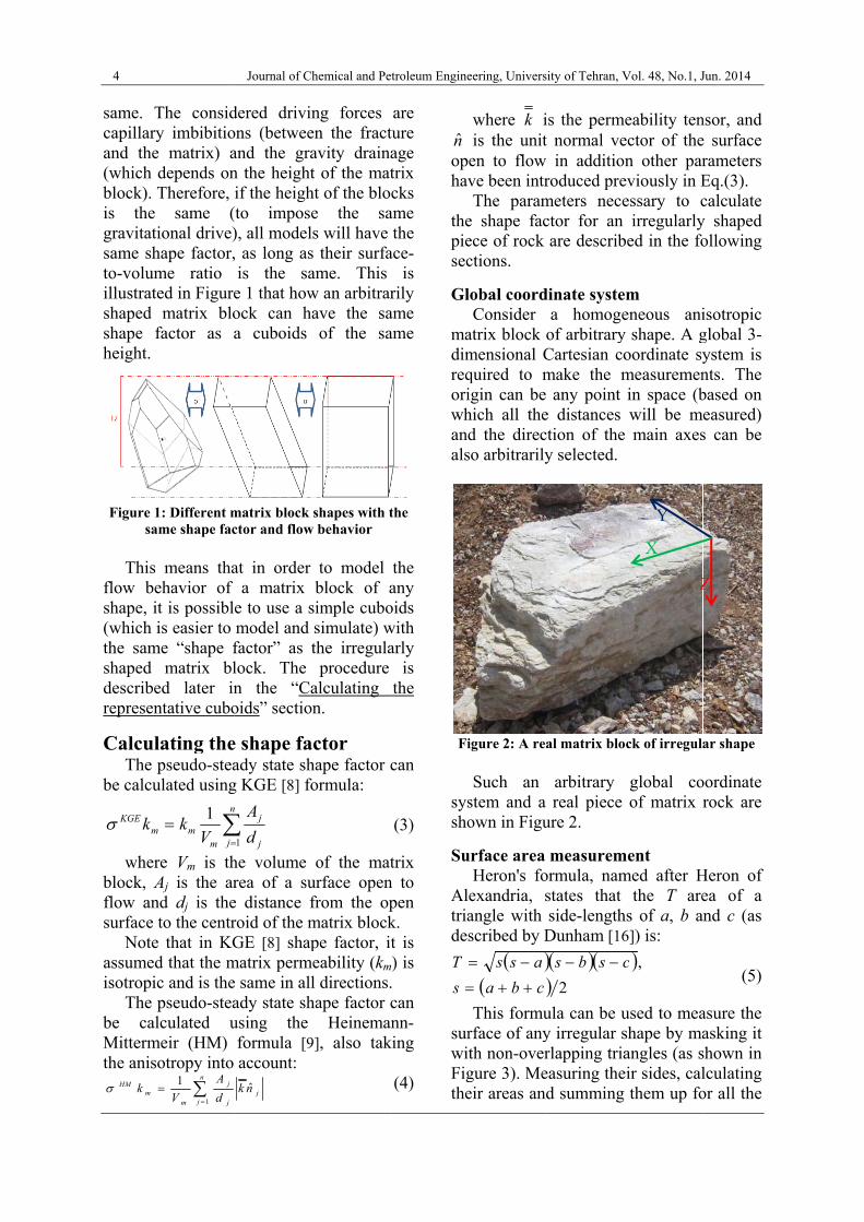
same. Tcapillaryand the(which block). is the gravitatsame shto-volumillustratshaped shape fheight.

Figure 1sa

This flow beshape, i(which the samshaped describerepresen

Calcul The be calcu

wherblock, Aflow ansurface Noteassumedisotropi The be calMittermthe anis

mKGE k

mHM k

The considy imbibitioe matrix) adepends onTherefore,

same (tional drive)hape factor,me ratio ted in Figure

matrix blofactor as a

1: Different mame shape fac

means thaehavior of it is possiblis easier to

me “shape fmatrix bl

ed later inntative cubo

lating thepseudo-stea

ulated using

re Vm is thAj is the arnd dj is theto the centr

e that in KGd that the mc and is thepseudo-stealculated u

meir (HM) sotropy into

n

jmmm V

k1

n

j j

j

m d

A

V 1

1

Journal of Ch

dered drivinons (betweeand the gran the heightif the heigh

(to impose), all model, as long asis the sae 1 that howock can haa cuboids

matrix block ctor and flow

at in order a matrix

e to use a smodel and factor” as tlock. The n the “Caoids” sectio

e shape faady state shg KGE [8] fo

he volume rea of a sue distance froid of the mGE [8] shap

matrix perme same in allady state shusing the formula [9account:

n

j

j

d

A

1

jnk ˆ

hemical and Pe

ng forces en the fractavity draint of the mat

ht of the bloe the sas will have

s their surfaame. This w an arbitrarave the saof the sa

shapes with tw behavior

to model block of a

simple cubosimulate) wthe irregulaprocedure

alculating n.

ctor hape factor cormula:

of the maturface openfrom the opmatrix blockpe factor, ieability (km

l directions.hape factor c

Heinema9], also tak

etroleum Engine

are ture age trix cks

ame the

ace-is

rily ame ame

the

the any oids with arly

is the

can

(3)

trix n to pen k. t is

m) is . can

ann-king

(4)

n̂ophav

thepiesec

Gl

madimreqoriwhandals

Fi

syssho

Su

Altriades

surwitFigthe

s

T

eering, Univers

where k iis the uniten to flow ve been intrThe param

e shape facece of rock ctions.

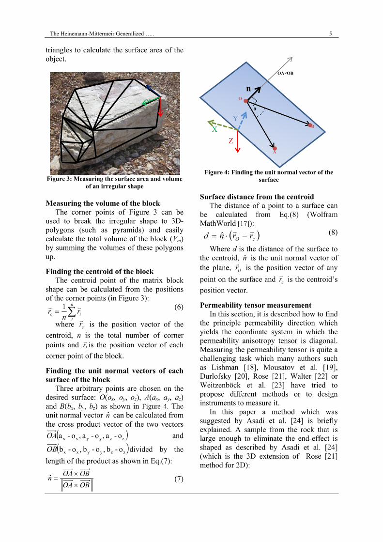
lobal coordConsider

atrix block omensional Cquired to migin can be hich all thed the direcso arbitrarily

igure 2: A rea

Such an stem and a own in Figu

urface area Heron's fo

exandria, sangle with scribed by D

This formurface of anyth non-overgure 3). Meeir areas and

cba

ass

ity of Tehran, V

is the permt normal ve

in additionroduced premeters necector for an are describ

dinate systea homoge

of arbitraryCartesian comake the m

any point e distances ction of they selected.

al matrix blo

arbitrary real piece

ure 2.

measuremormula, namstates that side-length

Dunham [16

ula can be uy irregular srlapping triaeasuring thed summing

2

csbs

Vol. 48, No.1, J

eability tenector of then other par

eviously in Eessary to c

irregularlybed in the fo

em eneous aniy shape. A goordinate symeasuremenin space (bwill be m

e main axes

ock of irregula

global coof matrix

ment med after H

the T arehs of a, b a6]) is:

used to meashape by maangles (as s

eir sides, calthem up fo

,c

X

Y

Z

Jun. 2014

nsor, and e surface rameters Eq.(3). calculate y shaped ollowing

isotropic global 3-ystem is nts. The based on easured) s can be

ar shape

oordinate rock are

Heron of ea of a

and c (as

(5)

asure the asking it shown in lculating or all the

Z

The Heinemann-Mittermeir Generalized ….. 5

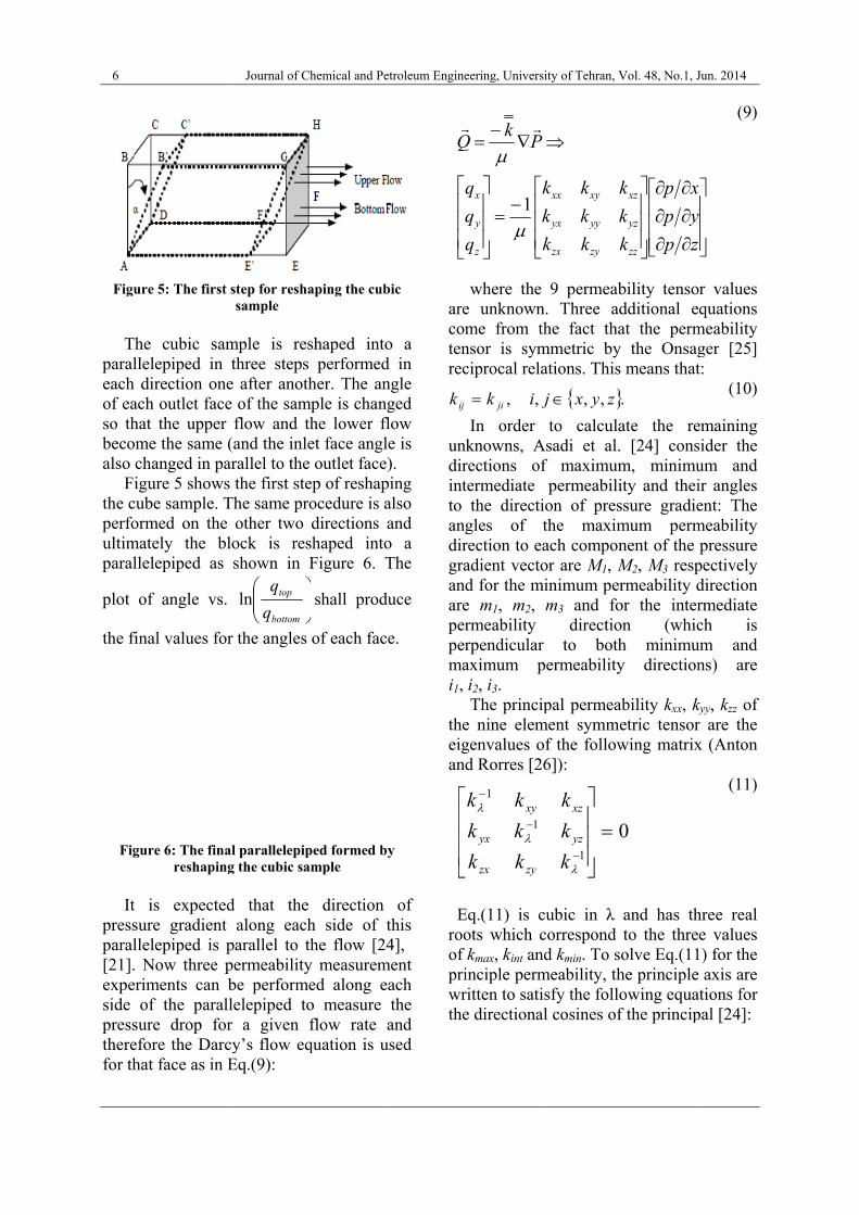
triangles to calculate the surface area of the object.

Figure 3: Measuring the surface area and volume

of an irregular shape Measuring the volume of the block The corner points of Figure 3 can be used to break the irregular shape to 3D-polygons (such as pyramids) and easily calculate the total volume of the block (Vm) by summing the volumes of these polygons up.

Finding the centroid of the block The centroid point of the matrix block shape can be calculated from the positions of the corner points (in Figure 3):

(6)

where cr

is the position vector of the

centroid, n is the total number of corner points and ir

is the position vector of each

corner point of the block.

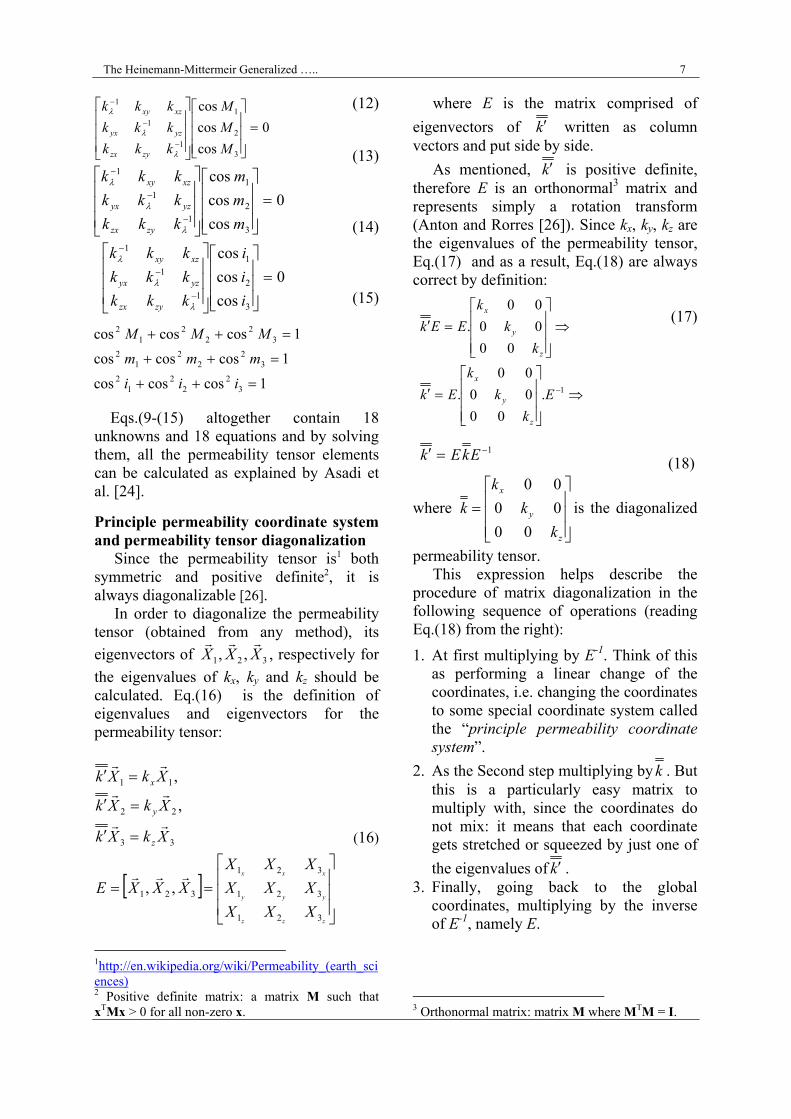
Finding the unit normal vectors of each surface of the block Three arbitrary points are chosen on the desired surface: O(ox, oy, oz), A(ax, ay, az) and B(bx, by, bz) as shown in Figure 4. The unit normal vector n̂ can be calculated from the cross product vector of the two vectors

zzyyxx o - a ,o - a ,o - aOA and

zzyyxx o - b ,o - b ,o - bOB divided by the

length of the product as shown in Eq.(7):

(7)

Figure 4: Finding the unit normal vector of the surface

Surface distance from the centroid The distance of a point to a surface can be calculated from Eq.(8) (Wolfram MathWorld [17]):

(8)

Where d is the distance of the surface to the centroid, n̂ is the unit normal vector of the plane, Or

is the position vector of any

point on the surface and cr

is the centroid’s

position vector.

Permeability tensor measurement In this section, it is described how to find the principle permeability direction which yields the coordinate system in which the permeability anisotropy tensor is diagonal. Measuring the permeability tensor is quite a challenging task which many authors such as Lishman [18], Mousatov et al. [19], Durlofsky [20], Rose [21], Walter [22] or Weitzenböck et al. [23] have tried to propose different methods or to design instruments to measure it. In this paper a method which was suggested by Asadi et al. [24] is briefly explained. A sample from the rock that is large enough to eliminate the end-effect is shaped as described by Asadi et al. [24] (which is the 3D extension of Rose [21] method for 2D):

XY

Z

OBOA

OBOAn

ˆ

n

iic r

nr

1

cO rrnd

ˆ

θ

n

A

O

B

OA×OB

Z

X

Y

6

Figure

The paralleleeach dirof each so that becomealso cha Figuthe cubeperformultimateparallele

plot of

the fina

Figure

It ispressureparallele[21]. Nexperimside of pressurethereforfor that

5: The first s

cubic samepiped in trection oneoutlet face the upper

e the same (anged in parure 5 shows e sample. T

med on the ely the bloepiped as

angle vs.

l values for

e 6: The finalreshaping

s expectede gradient epiped is pow three p

ments can bf the paralle drop for re the Darcyface as in E

Journal of Ch

step for reshasample

mple is resthree steps

e after anothof the samflow and thand the inlerallel to the the first ste

The same proother two ock is resshown in F

bottom

top

q

qln

r the angles

l parallelepipg the cubic sa

d that the along each

parallel to thermeability

be performeelepiped to

a given fy’s flow eq

Eq.(9):

hemical and Pe

aping the cub

shaped intoperformed

her. The anmple is chang

he lower flet face angloutlet face)

ep of reshapocedure is adirections a

shaped intoFigure 6. T

shall produ

of each face

ped formed bymple

direction h side of the flow [24

y measuremed along eao measureflow rate a

quation is u

etroleum Engine

bic

o a d in ngle ged low e is ).

ping also and o a The

uce

e.

y

of this 4],

ment ach the and

used

arecomtenrec

unkdirintto angdirgraandareperpermai1,

theeigand

Erooof priwrthe

q

q

q

Q

kij

eering, Univers

where the e unknownme from thnsor is symciprocal rela

In order knowns, Arections oftermediate

the directigles of trection to eaadient vectod for the me m1, m2, rmeability rpendicularaximum pi2, i3. The princip

e nine elemgenvalues od Rorres [26

Eq.(11) is cots which ckmax, kint an

inciple permritten to satie directiona

k

k

k

q

q

q

Pk

Q

z

y

x

1

1

1

kk

kk

kk

zyzx

yx

xy

,, jik ji

ity of Tehran, V

9 permeabn. Three adhe fact tha

mmetric by ations. This

to calculaAsadi et al.f maximumpermeabili

ion of presthe maximach componor are M1, M

minimum perm3 and fo

directior to bothpermeability

pal permeament symmeof the follow6]):

cubic in λ correspond d kmin. To so

meability, thsfy the follol cosines of

kkk

kkk

kkk

zyzx

yyyx

xyxx

01

k

k

k

yz

xz

,, zyxj

Vol. 48, No.1, J

bility tensodditional eat the perm the Onsag means that

ate the re [24] consm, minimuity and theissure gradiemum permnent of the M2, M3 resprmeability d

or the interon (which minimuy direction

ability kxx, ketric tensorwing matrix

and has thto the threolve Eq.(11he principleowing equaf the princip

zp

yp

xp

k

k

k

zz

yz

xz

0

.

Jun. 2014

(9)

r values quations

meability ger [25] t:

(10)

emaining sider the um and ir angles ent: The meability pressure

pectively direction rmediate ch is

um and ns) are

kyy, kzz of r are the x (Anton

(11)

hree real e values

1) for the axis are

ations for pal [24]:

x

The Heinemann-Mittermeir Generalized ….. 7

(12)

(13)

(14)

(15)

Eqs.(9-(15) altogether contain 18 unknowns and 18 equations and by solving them, all the permeability tensor elements can be calculated as explained by Asadi et al. [24].

Principle permeability coordinate system and permeability tensor diagonalization Since the permeability tensor is1 both symmetric and positive definite2, it is always diagonalizable [26]. In order to diagonalize the permeability tensor (obtained from any method), its

eigenvectors of 321 ,, XXX

, respectively for

the eigenvalues of kx, ky and kz should be calculated. Eq.(16) is the definition of eigenvalues and eigenvectors for the permeability tensor:

(16)

1http://en.wikipedia.org/wiki/Permeability_(earth_sciences) 2 Positive definite matrix: a matrix M such that xTMx > 0 for all non-zero x.

where E is the matrix comprised of

eigenvectors of k written as column vectors and put side by side.

As mentioned, k is positive definite, therefore E is an orthonormal3 matrix and represents simply a rotation transform (Anton and Rorres [26]). Since kx, ky, kz are the eigenvalues of the permeability tensor, Eq.(17) and as a result, Eq.(18) are always correct by definition:

(17)

(18)

where

z

y

x

k

k

k

k

00

00

00

is the diagonalized

permeability tensor. This expression helps describe the procedure of matrix diagonalization in the following sequence of operations (reading Eq.(18) from the right):

1. At first multiplying by E-1. Think of this as performing a linear change of the coordinates, i.e. changing the coordinates to some special coordinate system called the “principle permeability coordinate system”.

2. As the Second step multiplying by k . But this is a particularly easy matrix to multiply with, since the coordinates do not mix: it means that each coordinate gets stretched or squeezed by just one of

the eigenvalues of k . 3. Finally, going back to the global

coordinates, multiplying by the inverse of E-1, namely E.

3 Orthonormal matrix: matrix M where MTM = I.

zzz

yyy

xxx

XXX

XXX

XXX

XXXE

XkXk

XkXk

XkXk

z

y

x

321

321

321

321

33

22

11

,,

,

,

1.

00

00

00

.

00

00

00

.

E

k

k

k

Ek

k

k

k

EEk

z

y

x

z

y

x

1 EkEk

0

cos

cos

cos

3

2

1

1

1

1

M

M

M

kkk

kkk

kkk

zyzx

yzyx

xzxy

0

cos

cos

cos

3

2

1

1

1

1

m

m

m

kkk

kkk

kkk

zyzx

yzyx

xzxy

0

cos

cos

cos

3

2

1

1

1

1

i

i

i

kkk

kkk

kkk

zyzx

yzyx

xzxy

1coscoscos

1coscoscos

1coscoscos

32

22

12

32

22

12

32

22

12

iii

mmm

MMM

8 Journal of Chemical and Petroleum Engineering, University of Tehran, Vol. 48, No.1, Jun. 2014

Note that the order of choosing the eigenvalues as kx, ky or kz is not important, since the rotation matrix is created by the corresponding eigenvectors in the same order as the selected eigenvalues. In the other words, the values of the diagonalized permeability tensor in the transformed coordinate system will be always the same, regardless of the order of selection of the eigenvalues.

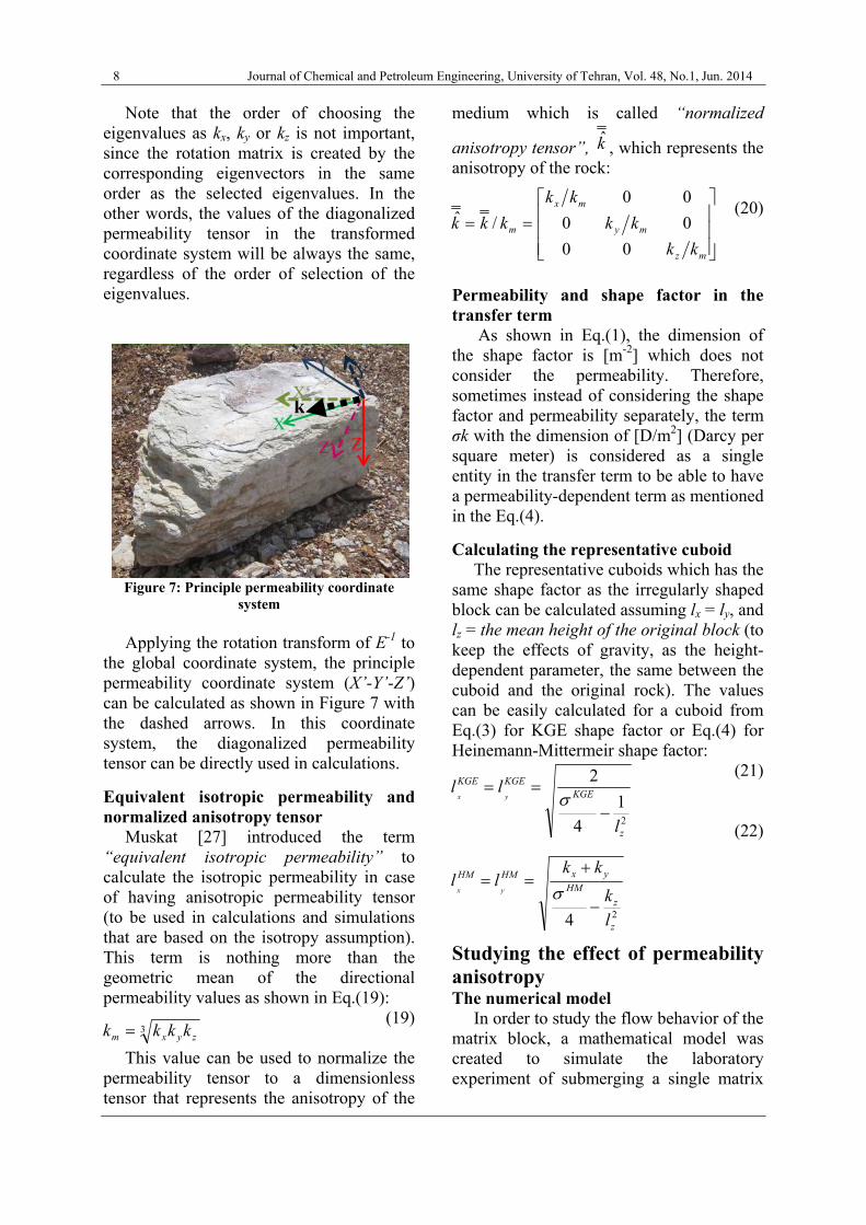
Figure 7: Principle permeability coordinate

system Applying the rotation transform of E-1 to the global coordinate system, the principle permeability coordinate system (X’-Y’-Z’) can be calculated as shown in Figure 7 with the dashed arrows. In this coordinate system, the diagonalized permeability tensor can be directly used in calculations.

Equivalent isotropic permeability and normalized anisotropy tensor Muskat [27] introduced the term “equivalent isotropic permeability” to calculate the isotropic permeability in case of having anisotropic permeability tensor (to be used in calculations and simulations that are based on the isotropy assumption). This term is nothing more than the geometric mean of the directional permeability values as shown in Eq.(19):

(19) This value can be used to normalize the permeability tensor to a dimensionless tensor that represents the anisotropy of the

medium which is called “normalized

anisotropy tensor”, k̂ , which represents the anisotropy of the rock:

(20)

Permeability and shape factor in the transfer term As shown in Eq.(1), the dimension of the shape factor is [m-2] which does not consider the permeability. Therefore, sometimes instead of considering the shape factor and permeability separately, the term σk with the dimension of [D/m2] (Darcy per square meter) is considered as a single entity in the transfer term to be able to have a permeability-dependent term as mentioned in the Eq.(4).

Calculating the representative cuboid The representative cuboids which has the same shape factor as the irregularly shaped block can be calculated assuming lx = ly, and lz = the mean height of the original block (to keep the effects of gravity, as the height-dependent parameter, the same between the cuboid and the original rock). The values can be easily calculated for a cuboid from Eq.(3) for KGE shape factor or Eq.(4) for Heinemann-Mittermeir shape factor:

(21)

(22) Studying the effect of permeability anisotropy The numerical model In order to study the flow behavior of the matrix block, a mathematical model was created to simulate the laboratory experiment of submerging a single matrix

k X‘

X

Y

ZZ‘

Y‘

2

1

4

2

z

KGEKGEKGE

l

llyx

24 z

z

HM

yxHMHM

l

k

kkll

yx

mz

my

mx

m

kk

kk

kk

kkk

00

00

00

/ˆ

3zyxm kkkk

The Heinemann-Mittermeir Generalized ….. 9

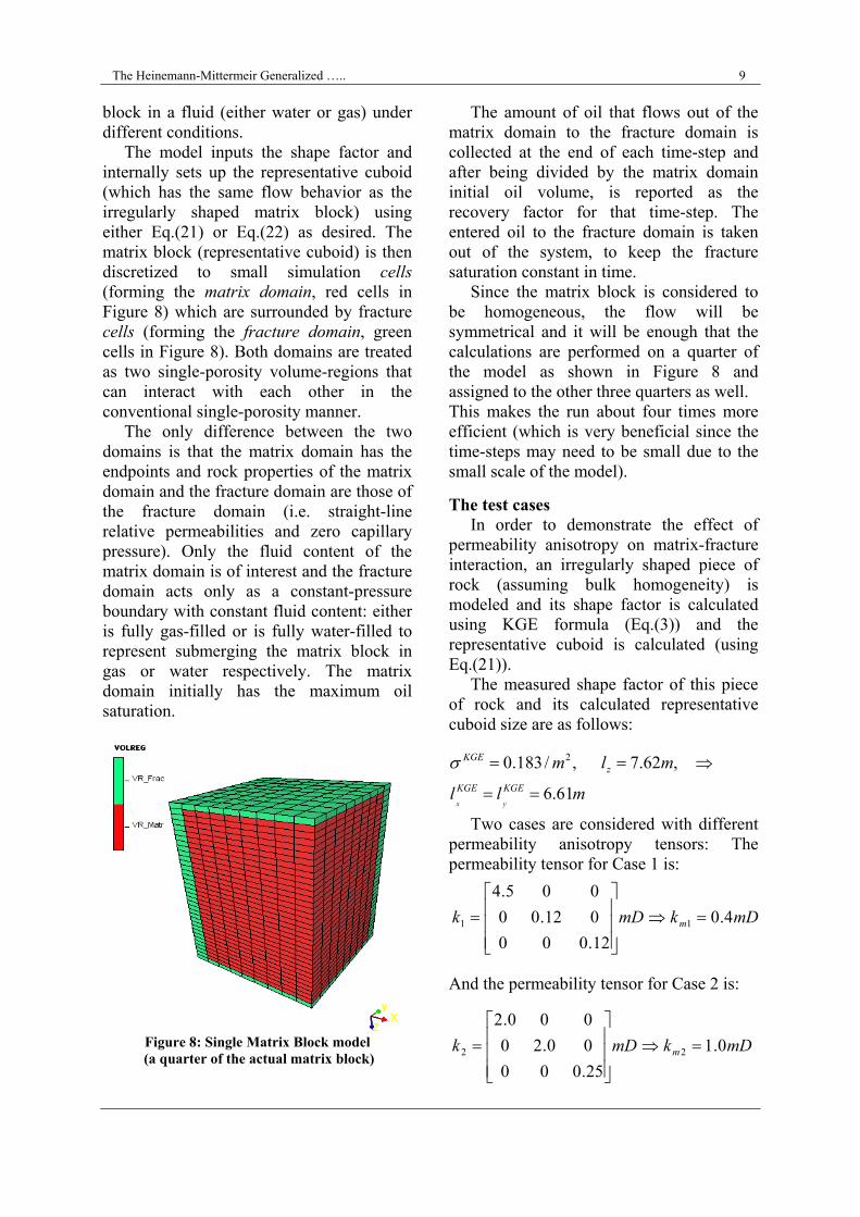
block in a fluid (either water or gas) under different conditions. The model inputs the shape factor and internally sets up the representative cuboid (which has the same flow behavior as the irregularly shaped matrix block) using either Eq.(21) or Eq.(22) as desired. The matrix block (representative cuboid) is then discretized to small simulation cells (forming the matrix domain, red cells in Figure 8) which are surrounded by fracture cells (forming the fracture domain, green cells in Figure 8). Both domains are treated as two single-porosity volume-regions that can interact with each other in the conventional single-porosity manner. The only difference between the two domains is that the matrix domain has the endpoints and rock properties of the matrix domain and the fracture domain are those of the fracture domain (i.e. straight-line relative permeabilities and zero capillary pressure). Only the fluid content of the matrix domain is of interest and the fracture domain acts only as a constant-pressure boundary with constant fluid content: either is fully gas-filled or is fully water-filled to represent submerging the matrix block in gas or water respectively. The matrix domain initially has the maximum oil saturation.

Figure 8: Single Matrix Block model

(a quarter of the actual matrix block)

The amount of oil that flows out of the matrix domain to the fracture domain is collected at the end of each time-step and after being divided by the matrix domain initial oil volume, is reported as the recovery factor for that time-step. The entered oil to the fracture domain is taken out of the system, to keep the fracture saturation constant in time. Since the matrix block is considered to be homogeneous, the flow will be symmetrical and it will be enough that the calculations are performed on a quarter of the model as shown in Figure 8 and assigned to the other three quarters as well. This makes the run about four times more efficient (which is very beneficial since the time-steps may need to be small due to the small scale of the model).

The test cases In order to demonstrate the effect of permeability anisotropy on matrix-fracture interaction, an irregularly shaped piece of rock (assuming bulk homogeneity) is modeled and its shape factor is calculated using KGE formula (Eq.(3)) and the representative cuboid is calculated (using Eq.(21)). The measured shape factor of this piece of rock and its calculated representative cuboid size are as follows: Two cases are considered with different permeability anisotropy tensors: The permeability tensor for Case 1 is: And the permeability tensor for Case 2 is:

mDkmDk m 4.0

12.000

012.00

005.4

11

mll

mlmKGEKGE

zKGE

yx61.6

,62.7,/183.0 2

mDkmDk m 0.1

25.000

00.20

000.2

22

10

The with mfracturecontainicapillarywater enoil out oil outflcollectedividingwill be that tim For scenario(while identica

(discretizedmaximum oe cells act ing alwaysy pressure nters the mto the fractlow of the m

ed from theg it by the

reported ame-step.

each peros for the p

all otheal):

Figure

Figure 10: A

Journal of C

d) matrix coil saturatas a bounds 100% wand gravity

matrix cells ature cells. Tmatrix in eae fracture cinitial matr

as the recov

rmeability permeabilityer parame

9: Time of re

Area and leng

AK

Chemical and P

cells are filtion, and dary condit

water. Due y drainage, and expels The amountch time-stepcells and arix oil contevery factor

tensor, ty are assumeters rem

ecovery vs. R

gth of the ma

Kmax

Petroleum Engin

lled the

tion to

the the

t of p is fter ent, r in

two med

main

1.

2.

FigrecbotCaisodaswit

Recovery facto

atrix block in

neering, Univer

The permeto the capermeabilitThe

permeabilitpermeabilitthe princisystem iscoordinate

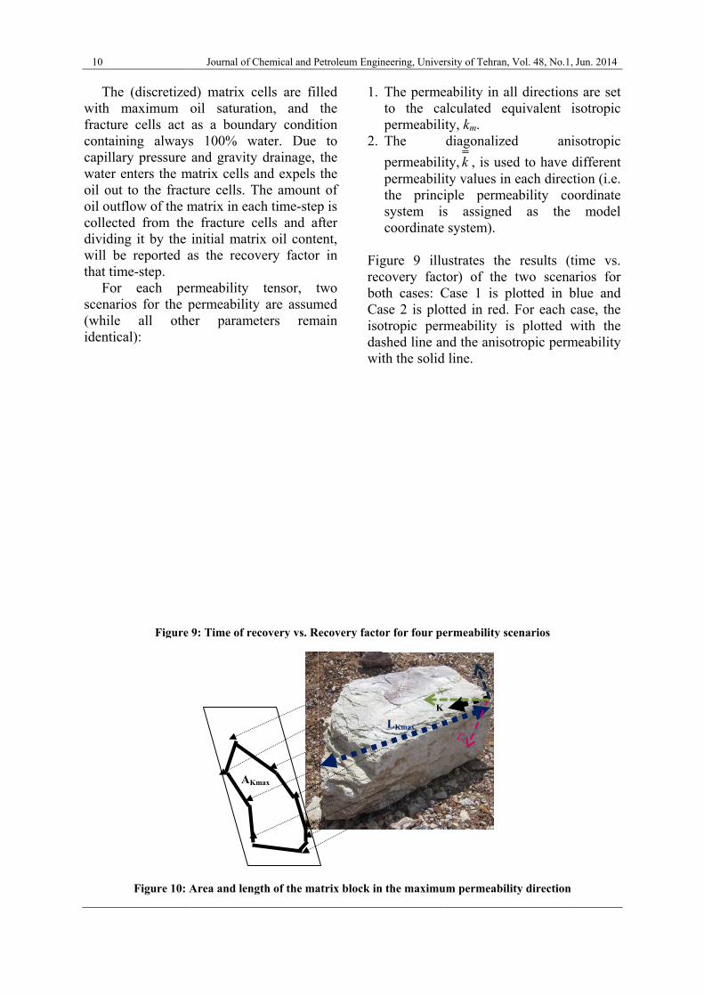
gure 9 illucovery factth cases: C

ase 2 is plototropic permshed line anth the solid

or for four pe

n the maximu

K

LKmax

X‘

rsity of Tehran,

eability in aalculated eqty, km. diagonalize

ty, k , is usety values iniple permes assignedsystem).

ustrates thetor) of the Case 1 is ptted in red.meability ind the anisoline.

ermeability sc

m permeabil

‘

Z‘

Y‘

Vol. 48, No.1,

all directionquivalent i

ed ani

ed to have dn each direceability cod as the

e results (ttwo scena

plotted in b For each cs plotted w

otropic perm

cenarios

lity direction

Jun. 2014

ns are set isotropic

isotropic

different tion (i.e.

oordinate model

time vs. arios for blue and case, the with the meability

The Heinemann-Mittermeir Generalized ….. 11

As can be observed, each scenario presents a completely different trend of recovery: 55% recovery of the matrix oil content for Case 1, takes nearly 8000 days (~22 years) with isotropy assumption while it takes about 21000 days (~58 years) considering the anisotropy. For Case 2 it takes about 3000 days (~8 years) with isotropy assumption and about 9000 days (~24 years) with anisotropy assumption. The difference in recovery time of 55% between the isotropic and anisotropic scenarios for Case 1 is ~36 years and for Case 2 is ~16 years which are quite remarkable differences in estimation of the recovery time from a small matrix block, with the same initial and boundary conditions only as a result of considering or ignoring the anisotropy. It is also observable that all the curves start at the same obvious recovery value of zero (while the initial conditions are the same) but also end at the same common recovery value of 64.68% as the ultimate recovery. The reason is that the ultimate recovery from the matrix block only depends on the driving mechanisms in action and the saturation endpoints, which are the same in all scenarios and are not dependent on the permeability. In the other words, all scenarios will ultimately produce the same amount of oil but with different trends and time scale. However, it is essential that this trend is known as accurate as possible to be able to make appropriate plans for the production from naturally fractured reservoirs.

Practical simplifications The presented method to measure the shape factor parameters from outcrops, is mathematically accurate, but may be considered too difficult to manually practice on a large scale/quantity. However, there are software programs that help make 3-dimensional models from the pieces of rock just by analyzing the pictures in different angles from the rock (such as 3D Software Object Modeller Pro [28]). These 3D models can be then used to

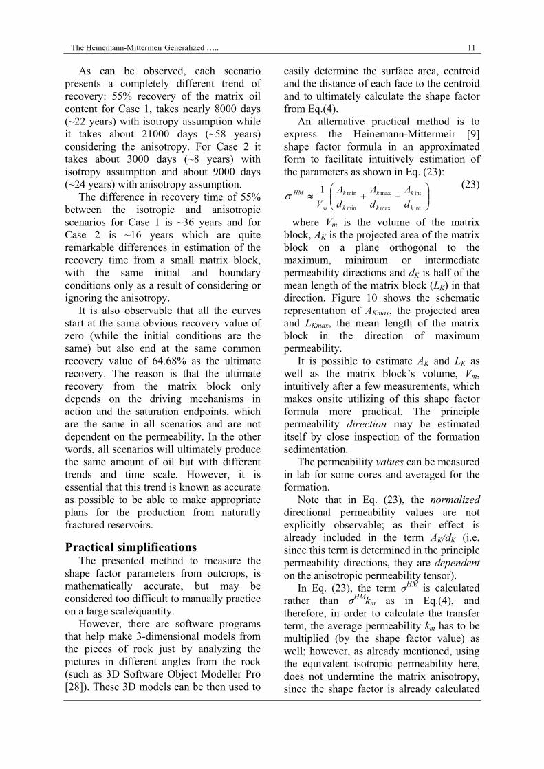
easily determine the surface area, centroid and the distance of each face to the centroid and to ultimately calculate the shape factor from Eq.(4). An alternative practical method is to express the Heinemann-Mittermeir [9] shape factor formula in an approximated form to facilitate intuitively estimation of the parameters as shown in Eq. (23):

(23) where Vm is the volume of the matrix block, AK is the projected area of the matrix block on a plane orthogonal to the maximum, minimum or intermediate permeability directions and dK is half of the mean length of the matrix block (LK) in that direction. Figure 10 shows the schematic representation of AKmax, the projected area and LKmax, the mean length of the matrix block in the direction of maximum permeability. It is possible to estimate AK and LK as well as the matrix block’s volume, Vm, intuitively after a few measurements, which makes onsite utilizing of this shape factor formula more practical. The principle permeability direction may be estimated itself by close inspection of the formation sedimentation. The permeability values can be measured in lab for some cores and averaged for the formation. Note that in Eq. (23), the normalized directional permeability values are not explicitly observable; as their effect is already included in the term AK/dK (i.e. since this term is determined in the principle permeability directions, they are dependent on the anisotropic permeability tensor). In Eq. (23), the term σHM is calculated rather than σHMkm as in Eq.(4), and therefore, in order to calculate the transfer term, the average permeability km has to be multiplied (by the shape factor value) as well; however, as already mentioned, using the equivalent isotropic permeability here, does not undermine the matrix anisotropy, since the shape factor is already calculated

int

int

max

max

min

min1

k

k

k

k

k

k

m

HM

d

A

d

A

d

A

V

12 Journal of Chemical and Petroleum Engineering, University of Tehran, Vol. 48, No.1, Jun. 2014

considering the normalized permeability tensor i.e. in the principle permeability direction. Such simplifications make it practical to use field outcrop investigations to measure the anisotropic shape factor more accurately than what is currently being used, but still not as time-consuming and as accurate as measuring all the parameters in the lab for every piece of rock, as was described earlier in this paper (which makes it impractical on a large scale).

Conclusions This study, using four different scenarios which were identical except for permeability tensor while follow completely different trends of production, demonstrates that although permeability anisotropy is not considered routinely in petroleum engineering studies, it can play a significant role in depletion trend of matrix blocks in naturally fractured reservoirs. Therefore, use of a shape factor such as Heinemann-Mittermeir which considers the anisotropy, also is theoretically derived and mathematically proven, is highly

recommended rather than using the simplified, commonly used Kazemi et al. isotropic shape factor which can result in quite wrong estimations of matrix depletion trend. Mathematical methods to determine all the parameters of Heinemann-Mittermeir shape factor for the matrix blocks of any shape (from the outcrops of fractured formations or elsewhere) were described and additionally, a possible simplified and more practical approach to intuitive estimation of those parameters was presented. It is suggested that field outcrop investigations should be performed for measuring the shape factor more accurate for the naturally fractured formations using the presented methods (especially in cases of high anisotropy). The test cases also suggest that using the apparent permeability in the transfer function which ignores the effect of anisotropy yet in a higher level than the shape factor, can be a more serious source of discrepancies in the matrix-fracture transfer rate calculation as well.

References: 1- Barenblatt, G. J., Zheltov, I. P. and Kochina, I. N. (1960). "Basic concepts in the theory of seepage of

homogeneous liquids in fissured rocks." J. Appl. Math. Mech., Vol. 24, pp. 1286-1303.

2- Warren, J.E. and Root, P.J. (1963). The Behavior of Naturally Fractured Reservoirs, SPE Journal, (Sept.

1963), 245-255.

3- Kazemi, H., Merrill, L.S., Porterfield, K.L. and Zeman, P.R. (1976). Numerical Simulation of Water-Oil Flow

in Naturally Fractured Reservoirs, SPE Journal, 317-326.

4- Coats, K.H. (1989). Implicit Compositional Simulation of Single-Porosity and Dual-Porosity Reservoirs. SPE

paper 18427.

5- Quintard, M. and Whitaker, S. (1996). "Theoretical development of region-averaged equations for slightly

compressible single-phase flow." Adv. Water Res., Vol. 19(1), pp. 29-47.

6- Zimmerman, R.W., Chen, G., Hadgu, T. and Bodvarsson, G.S. (1993). "A numerical dual-porosity model with

semi-analytical treatment of fracture/matrix flow." Wat. Resour. Res., Vol. 29(7), pp. 2127-2137.

7- Mathias, S.A. and Zimmerman, R.W. (2003). Laplace transform inversion for late-time behavior of

groundwater flow problems. Water Resources Research, 39(10): paper 1283.

8- Kazemi, H., Gilman, J.R. and Elsharkawy, A.M. (1992). Analytical and Numerical Solution of Oil Recovery

from Fractured Reservoirs Using Empirical Transfer Functions, SPE Reservoir Engineering, May 1992, 219-

227.

The Heinemann-Mittermeir Generalized ….. 13

9- Heinemann, Z.E. and Mittermeir, G.M. (2012). "Derivation of the Kazemi-Gilman-Elsharkawy generalized

dual porosity shape factor." Transp. Porous Med., Vol. 91(1), pp. 123-132.

10- de Swaan, A. (1976). Analytic Solutions for Determining Naturally Fracture Reservoir Properties by Well

Testing. SPE Paper, 5346-PA.

11- de Swaan, A. (1990). Influence of Shape and Skin of Matrix-Rock Blocks on Pressure Transients in

Fractured Reservoirs. SPE Formation Evaluation, Dec. 1990, 344-352.

12- Sarma, P. and Aziz, K. (2006). Production Optimization With Adjoint Models Under Nonlinear Control-

State Path Inequality Constraints. SPE Paper, 99959-MS.

13- Lim, KT. And Aziz, K. (1995). "Matrix-fracture transfer shape factors for dual-porosity simulators." J. Pet.

Sci. Eng, Vol. 13, pp. 169-178.

14- Schlumberger, (2012). ECLIPSE reservoir simulation software – Technical Description Version 2012.1.

15- Barker, J.A. (1985). "Block-geometry functions characterizing transport in densely fissured media." J.

Hydrol., Vol. 77, pp. 263-279.

16- Dunham, W. (1990). Heron's Formula for Triangular Area. Ch. 5 in Journey through Genius: The Great

Theorems of Mathematics. New York: Wiley, pp. 113-132.

17- Wolfram Math World, http://mathworld.wolfram.com/Point-PlaneDistance.html

18- Lishman, J.R. (1970). Core Permeability Anisotropy, J. Canadian Pet. Tech., 9(2).

19- Mousatov, A., Pervago, E. and Shevnin, V. (2000). A New Approach to Resistivity Anisotropy

Measurements, SEG 2000 Expanded Abstracts, 2000-1381.

20- Durlofsky, L.J. (1991). "Numerical calculation of equivalent grid block permeability tensors for

heterogeneous porous media." Wat. Resou. Res., Vol. 27(5), pp. 699-708.

21- Rose, W. (1982). "A new method to measure directional permeability." J. Petrol. Technol., May 1982.

22- Walter D., R. (1982). "A new method to measure directional permeability." J. Petrol. Eng., Vol. 34(5), pp.

1142-1144.

23- Weitzenböck, J.R., Shenoi, R.A. and Wilson, P.A. (1997). "Measurement of three-dimensional

permeability." Appl. Sci. Manuf., Vol. 29, pp. 159-169.

24- Asadi, M., Ghalambor, A., Rose, W.D. and Shirazi, M. K. (2000). Anisotropic Permeability Measurement of

Porous Media: A 3-Dimensional Method. SPE Conference Paper, 59396.

25- Onsager, L. (1931). "Reciprocal relations in irreversible processes." Phys. Rev. Vol. 37, pp. 405-426.

26- Anton, H. and Rorres, C. (2000). Elementary Linear Algebra (Applications Version) 8th edition, John Wiley

& Sons. ISBN 978-0-471-17052-5.

27- Muskat, M. (1937). The flow of homogeneous fluids through porous media, Mc Graw Hill Book Company

Inc., NY, USA, 137-148.

28- Creative Dimension Software Ltd – 3D Software Modeller Pro.