Embed Size (px)
Citation preview


Unified Fracture DesignBridging the Gap Between Theory and Practice


Unified Fracture DesignBridging the Gap Between Theory and Practice
Michael EconomidesRonald Oligney
Peter Valkó
Orsa Press
Alvin, Texas
Unified Fracture Design
Copyright © 2002 by Orsa Press
All rights, including reproduction by photographic or electronic process andtranslation into other languages are fully reserved under the InternationalCopyright Union, the Universal Copyright Convention, and the Pan-AmericanCopyright Convention. Reproduction of this book in whole or in part in anymanner without written permission from the publisher is prohibited.
Orsa PressP.O. Box 2569Alvin, TX 77512
10 9 8 7 6 5 4 3 2 1
Library of Congress Cataloging-in-Publication Data
Economides, Michael J.Unified fracture design : bridging the gap between theory and
practice / Michael Economides, Ronald Oligney, Peter Valkóp. cm.
Includes bibliographical references and index.ISBN 0-9710427-0-5 (alk. paper)1. Oil wells—Hydraulic fracturing. I. Oligney, Ronald E.
II. Valkó, Peter, 1950- III. Title.
TN871.E335 2002622'.3382—dc21 2002025793
Printed in the United States of America
Contents
v
CHAPTER 1Hydraulic Fracturing for Production
or Injection Enhancement 1
■ FRACTURING AS COMPLETION OF CHOICE 1■ BASIC PRINCIPLES OF UNIFIED FRACTURE DESIGN 4
Fractured Well Performance 5Sizing and Optimization 7
Fracture-to-Well Connectivity 8■ THE TIP SCREENOUT CONCEPT AND OTHER ISSUES
IN HIGH PERMEABILITY FRACTURING 9Tip Screenout Design 10
Net Pressure and Leakoff in the High Permeability Environment 11Candidate Selection 12
■ “BACK OF THE ENVELOPE” FRACTURE DESIGN 14Design Logic 14
Fracture Design Spreadsheet 14
CHAPTER 2How To Use This Book 17
■ STRUCTURE OF THE BOOK 17
■ WHICH SECTIONS ARE FOR YOU 18
Fracturing Crew 19
vi ■ Contents
CHAPTER 3Well Stimulation as a Means to Increase
the Productivity Index 23
■ PRODUCTIVITY INDEX 23■ THE WELL-FRACTURE-RESERVOIR SYSTEM 26
■ PROPPANT NUMBER 27Well Performance for Low and Moderate Proppant Numbers 32
■ OPTIMUM FRACTURE CONDUCTIVITY 35■ DESIGN LOGIC 38
CHAPTER 4Fracturing Theory 39
■ LINEAR ELASTICITY AND FRACTURE MECHANICS 39■ FRACTURING FLUID MECHANICS 42
■ LEAKOFF AND VOLUME BALANCE IN THE FRACTURE 46Formal Material Balance: The Opening-Time Distribution Factor 46
Constant Width Approximation (Carter Equation II) 48Power Law Approximation to Surface Growth 48
Detailed Leakoff Models 50
■ BASIC FRACTURE GEOMETRIES 50Perkins-Kern Width Equation 51
Khristianovich-Zheltov-Geertsma-deKlerk Width Equation 53Radial (Penny-shaped) Width Equation 54
CHAPTER 5Fracturing of High Permeability Formations 57
■ THE EVOLUTION OF THE TECHNIQUE 57■ HPF IN VIEW OF COMPETING TECHNOLOGIES 60
Gravel Pack 60High-Rate Water Packs 62
■ PERFORMANCE OF FRACTURED HORIZONTAL WELLSIN HIGH PERMEABILITY FORMATIONS 62

Contents ■ vii
■ DISTINGUISHING FEATURES OF HPF 63The Tip Screenout Concept 63
Net Pressure and Fluid Leakoff 66Net Pressure, Closure Pressure, and Width in Soft Formations 66
Fracture Propagation 66
■ LEAKOFF MODELS FOR HPF 67Fluid Leakoff and Spurt Loss as Material Properties: The Carter Leakoff
Model with Nolte’s Power Law Assumption 67Filter Cake Leakoff Model According to Mayerhofer, et al. 68
Polymer-Invaded Zone Leakoff Model of Fan and Economides 70
■ FRACTURING HIGH PERMEABILITY GAS CONDENSATE RESERVOIRS 72Optimizing Fracture Geometry in Gas Condensate Reservoirs 74
■ EFFECT OF NON-DARCY FLOW IN THE FRACTURE 76Definitions and Assumptions 77
Case Study for the Effect of Non-Darcy Flow 80
CHAPTER 6Fracturing Materials 83
■ FRACTURING FLUIDS 84■ FLUID ADDITIVES 85
■ PROPPANTS 87Calculating Effective Closure Stress 88
■ FRACTURE CONDUCTIVITY AND MATERIALS SELECTION IN HPF 91Fracture Width as a Design Variable 91
Proppant Selection 93Fluid Selection 94
CHAPTER 7Fracture Treatment Design 101
■ MICROFRACTURE TESTS 101■ MINIFRACS 102
■ TREATMENT DESIGN BASED ON THE UNIFIED APPROACH 109Pump Time 110
Proppant Schedule 113Departure from the Theoretical Optimum 118
TSO Design 119
viii ■ Contents
■ PUMPING A TSO TREATMENT 120Swab Effect Example 121Perforations for HPF 122
■ PRE-TREATMENT DIAGNOSTIC TESTS FOR HPF 122Step-Rate Tests 123
Minifracs 125Pressure Falloff Tests 126
Bottomhole Pressure Measurements 126
CHAPTER 8Fracture Design and Complications 129
■ FRACTURE HEIGHT 129Fracture Height Map 132
Practical Fracture Height Determination 133
■ TIP EFFECTS 134■ NON-DARCY FLOW IN THE FRACTURE 135
■ COMPENSATING FOR FRACTURE FACE SKIN 136■ EXAMPLES OF PRACTICAL FRACTURE DESIGN 137
A Typical Preliminary Design—Medium Permeability Formation: MPF01 137Pushing the Limit—Medium Permeability Formation: MPF02 142
Proppant Embedment: MPF03 145Fracture Design for High Permeability Formation: HPF01 148
Extreme High Permeability: HPF02 152Low Permeability Fracturing: LPF01 157
■ SUMMARY 162
CHAPTER 9Quality Control and Execution 163
■ FRACTURING EQUIPMENT 164■ EQUIPMENT LIST 166
Water Transfer and Storage 166Proppant Supply 167
Slurrification and Blending 168Pumping 169
Monitoring and QA/QC 172Miscellaneous 174
■ SPECIAL INSTRUCTIONS ON HOOK-UP 174Spotting the Equipment 174

Contents ■ ix
Fluid Supply-to-Blender 177Proppant Supply 177
Frac Pumps 177Manifold-to-Well 178
Monitoring/Control Equipment and Support Personnel 179
■ STANDARD FRACTURING QA PROCEDURES 180■ FORCED CLOSURE 181
■ QUALITY CONTROL FOR HPF 183
CHAPTER 10Treatment Evaluation 185
■ REAL-TIME ANALYSIS 185■ HEIGHT CONTAINMENT 186
■ LOGGING METHODS AND TRACERS 188■ A WORD ON FRACTURE MAPPING 189
■ WELL TESTING 190■ EVALUATION OF HPF TREATMENTS—A UNIFIED APPROACH 193
Production Results 193Evaluation of Real-Time HPF Treatment Data 194
Post-Treatment Well Tests in HPF 195Validity of the Skin Concept in HPF 197
■ SLOPES ANALYSIS 197Assumptions 198
Restricted Growth Theory 199Slopes Analysis Algorithms 201
AppendicesA: NOMENCLATURE 207
B: GLOSSARY 211
C: BIBLIOGRAPHY 219
D: FRACTURE DESIGN SPREADSHEET 227
E: MINIFRAC SPREADSHEET 233
F: STANDARD PRACTICES AND QC FORMS 239
G: SAMPLE FRACTURE PROGRAM 251
Index 259

The purpose of writing this book is to establish a unified design meth-odology for hydraulic fracture treatments, a long established wellstimulation activity in the petroleum and related industries. Few activ-ities in the industry hold such potential to improve well performanceboth profitably and reliably.
The word “unified” has been selected deliberately to denote both theintegration of all the highly diverse technological aspects of the process,but also to dispel the popular notion that there is one type of treatmentthat applies to low-permeability and another to high-permeability res-ervoirs. It is natural, even for experienced practitioners to think sobecause traditional targets have been low-permeability reservoirs whilethe fracturing of high-permeability formations has sprung from thegravel pack, sand control practice.
The key idea is that treatment sizes can be unified because theycan be best characterized by the dimensionless Proppant Number,which determines the theoretically optimum fracture dimensions atwhich the maximum productivity or injectivity index can be obtained.Technical constraints should be satisfied in such a way that the designdeparts from the theoretical optimum only to the necessary extent. Withthis approach, difficult topics such as high- versus low-permeability frac-turing, extensive height growth, non-Darcy flow, and proppant embed-ment are treated in a transparent and unified way, providing theengineer with a logical and coherent design procedure.
A design software package is included with the book.
Preface
xi

The authors’ backgrounds span the entire spectrum of technical,research, development, and field applications in practically all geo-graphic and reservoir type settings. It is their desire that this book findsits appropriate place in everyday practice.
xii ■ Preface
FRACTURING AS COMPLETION OF CHOICE
This book has the ambition to do something that has not been doneproperly before: to unite the gap between theory and practice in whatis arguably the most common stimulation/well completion techniquein petroleum production. Even more important, the book takes a newand ascendant position on the most critical link in the sequence ofevents in this type of well stimulation—the sizing and the designof hydraulic fracture treatments.
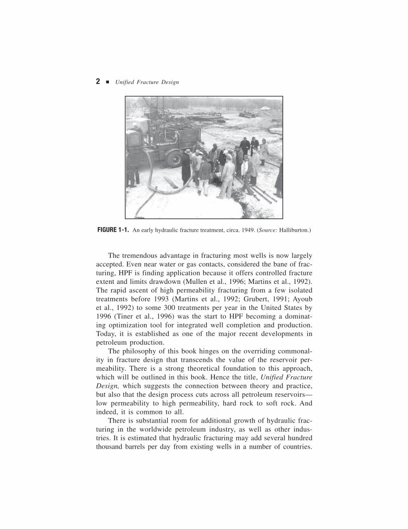
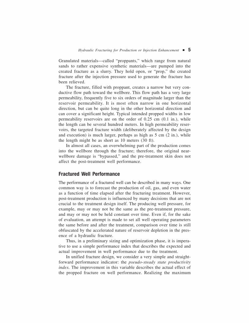
Fracturing was first employed to improve production from mar-ginal wells in Kansas in the late 1940s (Figure 1-1). Following anexplosion of the practice in the mid-1950s and a considerable surgein the mid-1980s, massive hydraulic fracturing (MHF) grew to becomea dominant completion technique, primarily for low permeability res-ervoirs in North America. By 1993, 40 percent of new oil wells and70 percent of gas wells in the United States were fracture treated.
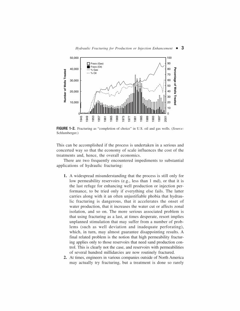
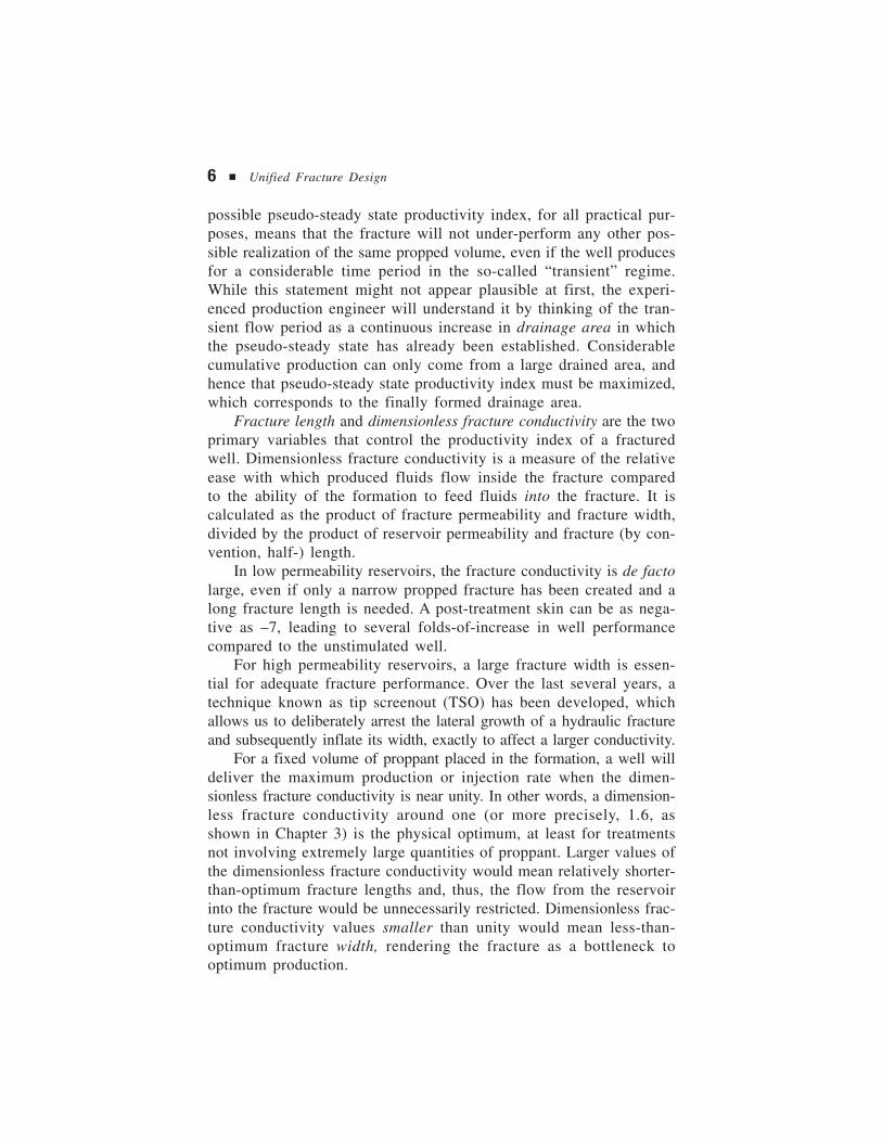
With improved modern fracturing capabilities and the advent ofhigh permeability fracturing (HPF), which in the vernacular has beenreferred to as “frac & pack” or variants, fracturing has expanded fur-ther to become the completion of choice for all types of wells in theUnited States, but particularly natural gas wells (see Figure 1-2).
Hydraulic Fracturing forProduction or InjectionEnhancement1
1
2 ■ Unified Fracture Design
The tremendous advantage in fracturing most wells is now largelyaccepted. Even near water or gas contacts, considered the bane of frac-turing, HPF is finding application because it offers controlled fractureextent and limits drawdown (Mullen et al., 1996; Martins et al., 1992).The rapid ascent of high permeability fracturing from a few isolatedtreatments before 1993 (Martins et al., 1992; Grubert, 1991; Ayoubet al., 1992) to some 300 treatments per year in the United States by1996 (Tiner et al., 1996) was the start to HPF becoming a dominat-ing optimization tool for integrated well completion and production.Today, it is established as one of the major recent developments inpetroleum production.
The philosophy of this book hinges on the overriding commonal-ity in fracture design that transcends the value of the reservoir per-meability. There is a strong theoretical foundation to this approach,which will be outlined in this book. Hence the title, Unified FractureDesign, which suggests the connection between theory and practice,but also that the design process cuts across all petroleum reservoirs—low permeability to high permeability, hard rock to soft rock. Andindeed, it is common to all.
There is substantial room for additional growth of hydraulic frac-turing in the worldwide petroleum industry, as well as other indus-tries. It is estimated that hydraulic fracturing may add several hundredthousand barrels per day from existing wells in a number of countries.
FIGURE 1-1. An early hydraulic fracture treatment, circa. 1949. (Source: Halliburton.)
Hydraulic Fracturing for Production or Injection Enhancement ■ 3
This can be accomplished if the process is undertaken in a serious andconcerted way so that the economy of scale influences the cost of thetreatments and, hence, the overall economics.
There are two frequently encountered impediments to substantialapplications of hydraulic fracturing:
1. A widespread misunderstanding that the process is still only forlow permeability reservoirs (e.g., less than 1 md), or that it isthe last refuge for enhancing well production or injection per-formance, to be tried only if everything else fails. The lattercarries along with it an often unjustifiable phobia that hydrau-lic fracturing is dangerous, that it accelerates the onset ofwater production, that it increases the water cut or affects zonalisolation, and so on. The more serious associated problem isthat using fracturing as a last, at times desperate, resort impliesunplanned stimulation that may suffer from a number of prob-lems (such as well deviation and inadequate perforating),which, in turn, may almost guarantee disappointing results. Afinal related problem is the notion that high permeability fractur-ing applies only to those reservoirs that need sand production con-trol. This is clearly not the case, and reservoirs with permeabilitiesof several hundred millidarcies are now routinely fractured.
2. At times, engineers in various companies outside of North Americamay actually try fracturing, but a treatment is done so rarely
FIGURE 1-2. Fracturing as “completion of choice” in U.S. oil and gas wells. (Source:Schlumberger.)
0
10,000
20,000
30,000
40,000
1945
1949
1953
1957
1961
1965
1969
1973
1977
1981
1985
1989
1993
1997
50,000
2001
0
10
20
30
40
50
60
70
80
90
100
Fracs (Gas)Fracs (Oil)% Gas% Oil
Nu
mb
er o
f W
ells
Tre
ated
Percen
tage o
f Wells T
reated
4 ■ Unified Fracture Design
and so haphazardly that it is bound to be expensive, such thatthe cost cannot be justified even if the incremental productionis substantial. Hydraulic fracturing is a massive operation with avery large complement of equipment, complicated and demand-ing fluids and proppants, and a wide spectrum of ancillary andpeople-intensive engineering and operational demands. Costsassigned to individual, isolated jobs—e.g., one or two treatmentscarried out every three to six months—are essentially prohibitive.Coupled with an occasional job failure, sketchy and spottyapplication of hydraulic fracturing is almost assured of economicfailure and the dampening of any desire to apply it further.
Virtually no petroleum operation carries such a differential pricetag among areas where it is applied in a widespread and massive way,such as North America and offshore in the North Sea, and elsewhere. InNorth America, over 60 percent of all oil wells and 85 percent of allgas wells are hydraulically fractured, and the percentages are stillincreasing. Yet, consider this: a 100-ton proppant treatment in theUnited States, at the time of this writing, costs less than $100,000.Exactly the same treatment, with the same equipment and the sameservice company, for example in Venezuela or Oman, is likely to costat least $1 million, and it can cost as much as $2 million.
At the same time, virtually no other petroleum technology carriesa larger incremental asset. The hundreds-of-thousands to millions ofbarrels per day of worldwide production increase that we projectassumes that the percentage of existing wells being hydraulically frac-tured approaches that of oil wells in the United States (60 percent),and the incremental production realized from each well is just 25percent over the pre-treatment state. The latter implies the very mod-est assumptions that all existing wells continue to produce, and thatfracturing would result in a very achievable average “skin” equal to–2. In fact, the incremental production capacity from a massive stimu-lation campaign with adequate equipment and well-trained people islikely to be much higher.
BASIC PRINCIPLES OF UNIFIED FRACTURE DESIGN
Hydraulic fracturing entails injecting fluids in an underground formationat a pressure that is high enough to induce a parting of the formation.
Hydraulic Fracturing for Production or Injection Enhancement ■ 5
Granulated materials—called “proppants,” which range from naturalsands to rather expensive synthetic materials—are pumped into thecreated fracture as a slurry. They hold open, or “prop,” the createdfracture after the injection pressure used to generate the fracture hasbeen relieved.
The fracture, filled with proppant, creates a narrow but very con-ductive flow path toward the wellbore. This flow path has a very largepermeability, frequently five to six orders of magnitude larger than thereservoir permeability. It is most often narrow in one horizontaldirection, but can be quite long in the other horizontal direction andcan cover a significant height. Typical intended propped widths in lowpermeability reservoirs are on the order of 0.25 cm (0.1 in.), whilethe length can be several hundred meters. In high permeability reser-voirs, the targeted fracture width (deliberately affected by the designand execution) is much larger, perhaps as high as 5 cm (2 in.), whilethe length might be as short as 10 meters (30 ft).
In almost all cases, an overwhelming part of the production comesinto the wellbore through the fracture; therefore, the original near-wellbore damage is “bypassed,” and the pre-treatment skin does notaffect the post-treatment well performance.
Fractured Well Performance
The performance of a fractured well can be described in many ways. Onecommon way is to forecast the production of oil, gas, and even wateras a function of time elapsed after the fracturing treatment. However,post-treatment production is influenced by many decisions that are notcrucial to the treatment design itself. The producing well pressure, forexample, may or may not be the same as the pre-treatment pressure,and may or may not be held constant over time. Even if, for the sakeof evaluation, an attempt is made to set all well operating parametersthe same before and after the treatment, comparison over time is stillobfuscated by the accelerated nature of reservoir depletion in the pres-ence of a hydraulic fracture.
Thus, in a preliminary sizing and optimization phase, it is impera-tive to use a simple performance index that describes the expected andactual improvement in well performance due to the treatment.
In unified fracture design, we consider a very simple and straight-forward performance indicator: the pseudo-steady state productivityindex. The improvement in this variable describes the actual effect ofthe propped fracture on well performance. Realizing the maximum
6 ■ Unified Fracture Design
possible pseudo-steady state productivity index, for all practical pur-poses, means that the fracture will not under-perform any other pos-sible realization of the same propped volume, even if the well producesfor a considerable time period in the so-called “transient” regime.While this statement might not appear plausible at first, the experi-enced production engineer will understand it by thinking of the tran-sient flow period as a continuous increase in drainage area in whichthe pseudo-steady state has already been established. Considerablecumulative production can only come from a large drained area, andhence that pseudo-steady state productivity index must be maximized,which corresponds to the finally formed drainage area.
Fracture length and dimensionless fracture conductivity are the twoprimary variables that control the productivity index of a fracturedwell. Dimensionless fracture conductivity is a measure of the relativeease with which produced fluids flow inside the fracture comparedto the ability of the formation to feed fluids into the fracture. It iscalculated as the product of fracture permeability and fracture width,divided by the product of reservoir permeability and fracture (by con-vention, half-) length.
In low permeability reservoirs, the fracture conductivity is de factolarge, even if only a narrow propped fracture has been created and along fracture length is needed. A post-treatment skin can be as nega-tive as –7, leading to several folds-of-increase in well performancecompared to the unstimulated well.
For high permeability reservoirs, a large fracture width is essen-tial for adequate fracture performance. Over the last several years, atechnique known as tip screenout (TSO) has been developed, whichallows us to deliberately arrest the lateral growth of a hydraulic fractureand subsequently inflate its width, exactly to affect a larger conductivity.
For a fixed volume of proppant placed in the formation, a well willdeliver the maximum production or injection rate when the dimen-sionless fracture conductivity is near unity. In other words, a dimension-less fracture conductivity around one (or more precisely, 1.6, asshown in Chapter 3) is the physical optimum, at least for treatmentsnot involving extremely large quantities of proppant. Larger values ofthe dimensionless fracture conductivity would mean relatively shorter-than-optimum fracture lengths and, thus, the flow from the reservoirinto the fracture would be unnecessarily restricted. Dimensionless frac-ture conductivity values smaller than unity would mean less-than-optimum fracture width, rendering the fracture as a bottleneck tooptimum production.
Hydraulic Fracturing for Production or Injection Enhancement ■ 7
There are a number of secondary issues that complicate the picture—early time transient flow regime, influence of reservoir boundaries,non-Darcy flow effects, and proppant embedment, just to mention afew. Nevertheless, these effects can be correctly taken into accountonly if the role of dimensionless fracture conductivity is understood.
It is possible that in certain theaters of operation the practicaloptimum may be different than the physical optimum. In some cases,the theoretically indicated fracture geometry may be difficult toachieve because of physical limitations imposed either by the avail-able equipment, limits in the fracturing materials, or the mechanicalproperties of the rock to be fractured. However, aiming to maximizethe well productivity or injectivity is an appropriate first step in thefracture design.
Sizing and Optimization
The term “optimum” as used above means the maximization of awell’s productivity, within the constraint of a certain treatment size.Hence, a decision on treatment size should actually precede (or gohand-in-hand with) an optimization based on the dimensionless frac-ture conductivity criterion.
For a long time, practitioners considered fracture half-length as aconvenient variable to characterize the size of the created fracture. Thattradition emerged because it was not possible to independently changefracture length and width, and because length had a primary effect onproductivity in low permeability formations. In unified fracture design,where both low and high permeability formations are considered, thebest single variable to characterize the size of a created fracture isthe volume of proppant placed in the productive horizon, or “pay.”
Obviously, the total volume of proppant placed in the pay inter-val is always less than the total proppant injected. From a practicalpoint of view, treatment sizing means deciding how much proppantto inject. When sizing the treatment, an engineer must be aware thatincreasing the injected amount of proppant by a certain quantity x willnot necessarily increase the amount of proppant reaching the pay layerby the same quantity, x. We will refer to the ratio of the two proppantvolumes (i.e., the volume of proppant placed in the pay intervaldivided by the total volume injected into the well) as the volumetricproppant efficiency.
By far the most critical factor in determining volumetric proppantefficiency is the ratio of created fracture height to the net pay thickness.

8 ■ Unified Fracture Design
Extensive height growth limits the volumetric proppant efficiency, andis something that we generally try to avoid. (The possibility of inter-secting a nearby water table is another important reason to avoidexcessive height growth.)
Actual selection of the amount of proppant indicated for injectionis primarily based on economics, the most commonly used criterionbeing the net present value (NPV). As with most engineering activi-ties, costs increase almost linearly with the size of the treatment, butafter a certain point, the revenues increase only marginally. Thus, thereis an optimum treatment size, the point at which the NPV of incre-mental revenue, balanced against treatment costs, is a maximum.
The optimum size can be determined if some method is availableto predict the maximum possible productivity increase achievable witha certain amount of proppant. Unified fracture design makes exten-sive use of this fact, given that the maximum achievable productivityincrease is already determined by the volume of proppant in the pay.Many of the operational details are subsumed by the basic decisionon treatment size, making possible a simple yet robust design process.
Therefore, we employ the concept of “volume of proppant reachingthe pay” or simply “propped volume in the pay” as the key decisionvariable in the sizing phase of the unified fracture design procedure.To handle it correctly, the amount of proppant indicated for injectionand the volumetric proppant efficiency must be determined.
Fracture-to-Well Connectivity
While the maximum achievable improvement of productivity is deter-mined by the propped volume in the pay, several additional conditionsmust be satisfied en route to a fracture that actually realizes thispotential improvement. One of the crucial factors is to establish anoptimum compromise between the length and width (or to depart fromthe optimum only as much as necessary, if required by operationalconstraints). As previously explained, the optimum dimensionless frac-ture conductivity is the variable that helps us to find the right com-promise. However, another condition is equally important. It is relatedto the connectivity of the fracture to the well.
A reservoir at depth is under a state of stress that can be charac-terized by three principal stresses: one vertical, which in almost allcases of deep reservoirs (depth greater than 500 meters, 1500 ft) isthe largest of the three, and two horizontal, one minimum and onemaximum. A hydraulic fracture will be normal to the smallest stress,
Hydraulic Fracturing for Production or Injection Enhancement ■ 9
leading to vertical hydraulic fractures in almost all petroleum produc-tion applications. The azimuth of these fractures is pre-ordained bythe natural state of earth stresses. As such, deviated or horizontal wellsthat are to be fractured should be drilled in an orientation that agreeswith this azimuth. Vertical wells, of course, naturally coincide withthe fracture plane.
If the well azimuth does not coincide with the fracture plane, thefracture is likely to initiate in one plane and then twist, causing con-siderable “tortuosity” en route to its final azimuth—normal to theminimum stress direction. Vertical wells with vertical fractures orperfectly horizontal wells drilled deliberately along the expected frac-ture plane result in the best aligned well-fracture systems. Other well-fracture configurations are subject to “choke effects,” unnecessarilydecreasing the productivity of the fractured well. Perforations and theirorientation may also be a source of problems during the execution ofa treatment, including multiple fracture initiations and prematurescreenouts caused by tortuosity effects.
The dimensionless fracture conductivity in low permeability reservoirsis naturally high, so the impact of choke effects from the phenomenadescribed above is generally minimized; to avoid tortuosity, pointsource fracturing is frequently employed.
Fracture-to-well connectivity is considered today as a critical pointin the success of high permeability fracturing, often dictating the wellazimuth (e.g., drilling S-shape vertical wells) or indicating horizontalwells drilled longitudinal to the fracture direction. Perforating is be-ing revisited, and alternatives, such as hydro-jetting of slots, are con-sidered by the most advanced practitioners. While some modelsincorporate complex well-fracture geometries with choke and othereffects, the many uncertainties prevent us from predicting performance.Rather, we are limited to explain the performance once post-treatmentwell test and production information become available. In the designphase, we try to make decisions that minimize the likelihood of suchunnecessary reductions in productivity.
THE TIP SCREENOUT CONCEPT AND OTHER ISSUESIN HIGH PERMEABILITY FRACTURING
Because high permeability fracturing has the most fertile possibilityfor expansion in petroleum operations worldwide, key issues for this

10 ■ Unified Fracture Design
type of well completion are described below. The purpose is to iden-tify those features that distinguish high permeability fracturing fromconventional hydraulic fracturing.
Tip Screenout Design
The critical elements of high permeability fracturing treatment design,execution and treatment behavioral interpretation are substantiallydifferent than for conventional fracturing treatments. In particular, HPFrelies on a carefully timed “tip screenout,” or TSO, to limit fracturegrowth and allow for fracture inflation and packing. The TSO occurswhen sufficient proppant has concentrated at the leading edge of thefracture to prevent further fracture extension. Once the fracture growthhas been arrested (and assuming the pump rate is larger than the rateof leakoff to the formation), continued pumping will inflate the frac-ture, i.e., increase the fracture width. Tip screenout and fracture in-flation should be accompanied by an increase in net fracturingpressure. Thus, the treatment can be conceptualized in two distinctstages: fracture creation (equivalent to conventional designs) and frac-ture inflation/packing (after tip screenout).
Creation of the fracture and arrest of its growth (i.e., the tip screen-out) is accomplished by injecting a relatively small “pad” of cleanfluid (no sand) followed by a “slurry” containing 1–4 lbs of sand pergallon of fluid (ppg). Once the fracture growth has been arrested,further injection builds fracture width and allows injection of a high-concentration slurry (e.g., 10–16 ppg). Final areal proppant concen-trations of 20 lbm/sq ft are possible. A usual practice is to retard theinjection rate near the end of the treatment (coincidental with open-ing the annulus to flow) to dehydrate and pack the fracture near thewell. Rate reductions may also be used to force a tip screenout in caseswhere no TSO event is observed on the downhole pressure record.
Frequent field experience suggests that the tip screenout can bedifficult to model, affect, or even detect. There are many reasons forthis, including a tendency toward overly conservative design models(resulting in no TSO), partial or multiple tip screenout events, andinadequate pressure monitoring practices.
Accurate bottomhole measurements are imperative for meaning-ful treatment evaluation and diagnosis. Calculated bottomhole pres-sures are unreliable because of the sizeable and complex frictionpressure effects associated with pumping high proppant slurry concen-trations through small diameter tubulars and service tool crossovers.
Hydraulic Fracturing for Production or Injection Enhancement ■ 11
Surface data may indicate that a TSO event has occurred when thebottomhole data shows no evidence, and vice versa.
Net Pressure and Leakoff in theHigh Permeability Environment
The entire HPF process is dominated by net pressure and fluid leakoffconsiderations. First, high permeability formations are typically softand exhibit low elastic modulus values, and second, the fluid volumesare relatively small and leakoff rates high (high permeability, com-pressible reservoir fluids and non-wall building fracturing fluids).While traditional practices applicable to design, execution, and evalu-ation in hydraulic fracturing continue to be used in HPF, these arefrequently not sufficient.
Net Pressure
Net pressure is the difference between the pressure at any point in thefracture and the pressure at which the fracture will close. This defini-tion implies the existence of a unique closure pressure. Whether theclosure pressure is a constant property of the formation or dependsheavily on the pore pressure (or rather on the disturbance of the porepressure relative to the long-term steady value) is an open question.
In high-permeability, soft formations it is difficult (if not impos-sible) to suggest a simple recipe to determine the closure pressure asclassically derived from shut-in pressure decline curves. Furthermore,because of the low elastic modulus values, even small induced uncer-tainties in the net pressure are amplified into large uncertainties in thecalculated fracture width.
Fracture propagation, the availability of sophisticated 3D modelsnotwithstanding, is a very complex process and difficult to describe,even in the best of cases, because of the large number and often com-peting physical phenomena. The physics of fracture propagation in softrock is even more complex, but it is reasonably expected to involveincremental energy dissipation and more severe tip effects when com-pared to hard rock fracturing. Again, because of the low modulusvalues, an inability to predict net pressure behavior may lead to a sig-nificant departure between predicted and actual treatment performance.Ultimately, the classic fracture propagation models may not reflect eventhe main features of the propagation process in high permeability rocks.

12 ■ Unified Fracture Design
It is common practice for some practitioners to “predict” fracturepropagation and net pressure features ex post facto using a computerfracture simulator. The tendency toward substituting clear models andphysical assumptions with “knobs”—e.g., arbitrary stress barriers,friction changes (attributed to erosion if decreasing and sand resis-tance if increasing) and less than well understood properties ofthe formation expressed as dimensionless factors—does not help toclarify the issue. Other techniques are warranted and several areunder development.
Leakoff
Considerable effort has been expended on laboratory investigation ofthe fluid leakoff process for high permeability cores. The results raisesome questions about how effectively fluid leakoff can be limited byfiltercake formation. In all cases, but especially in high permeabilityformations, the quality of the fracturing fluid is only one of thefactors that influence leakoff, and often not the determining one. Tran-sient fluid flow in the formation might have an equal or even largerimpact. Transient flow cannot be understood by simply fitting an em-pirical equation to laboratory data. The use of models based onsolutions to the fluid flow in porous media is an unavoidable step,and one that has already been taken by many.
Candidate Selection
The utility of high permeability fracturing extends beyond the obvi-ous productivity benefits associated with bypassing near-well damageto include sand control. However, in HPF the issue is not mere sandcontrol, which implies most often mechanical retention of migratingsand particles (and plugging), but rather sand deconsolidation control.
Increasingly, wellbore stability should be viewed in a holisticapproach with horizontal wells and hydraulic fracture treatments. Pro-active well completion strategies are critical to wellbore stability andsand-production control to reduce pressure drawdown while obtainingeconomically attractive rates. Reservoir candidate recognition for thecorrect well configurations is the key element. Necessary steps incandidate selection include appropriate reservoir engineering, forma-tion characterization, wellbore stability calculations, and the combiningof production forecasts with assessments of sand-production potential.
Hydraulic Fracturing for Production or Injection Enhancement ■ 13
Complex Well-Fracture Configurations
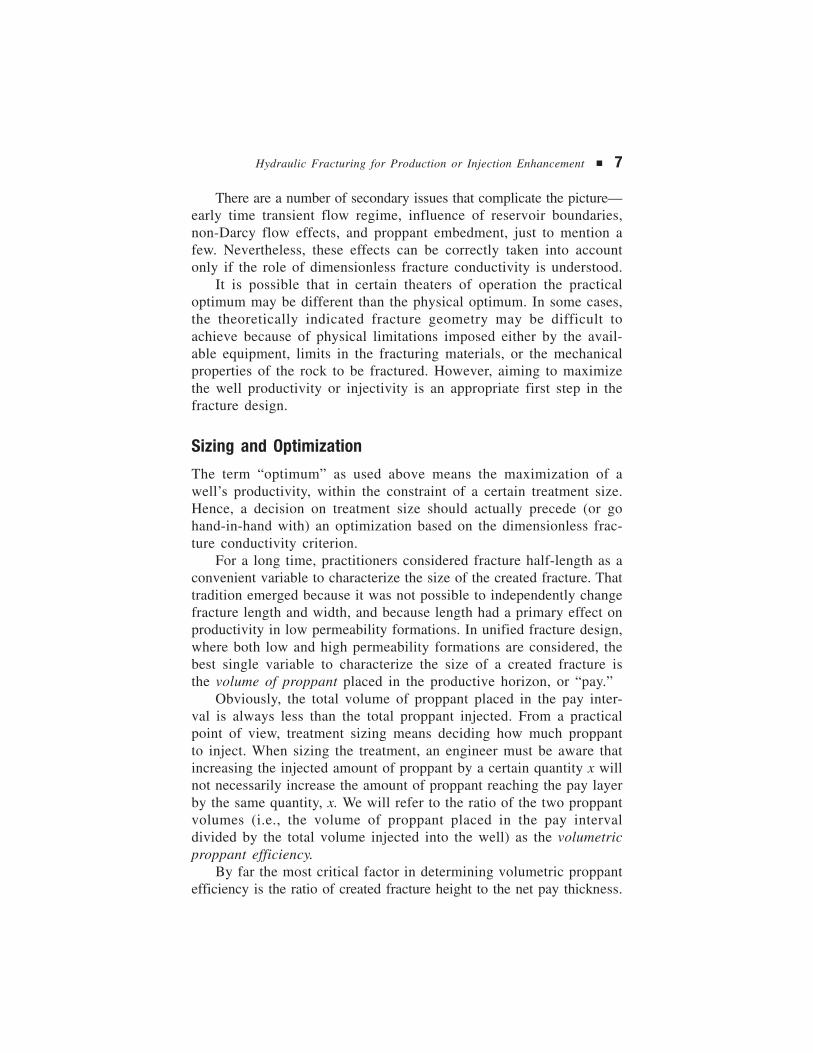
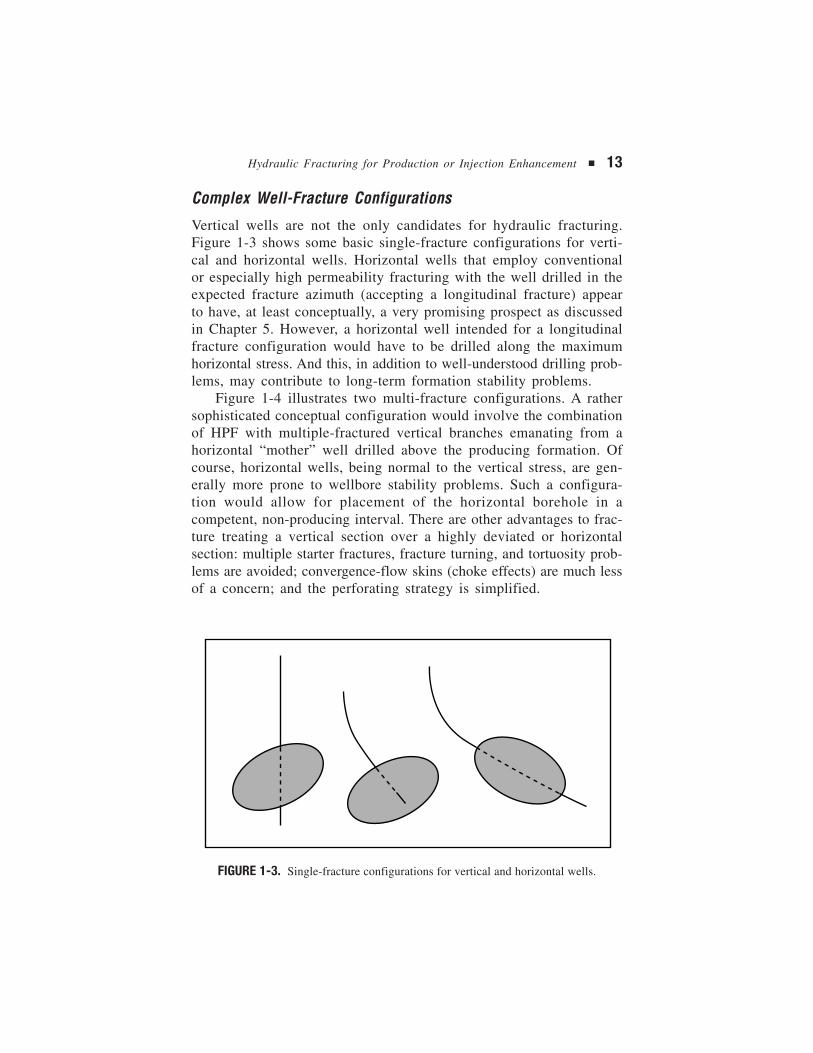
Vertical wells are not the only candidates for hydraulic fracturing.Figure 1-3 shows some basic single-fracture configurations for verti-cal and horizontal wells. Horizontal wells that employ conventionalor especially high permeability fracturing with the well drilled in theexpected fracture azimuth (accepting a longitudinal fracture) appearto have, at least conceptually, a very promising prospect as discussedin Chapter 5. However, a horizontal well intended for a longitudinalfracture configuration would have to be drilled along the maximumhorizontal stress. And this, in addition to well-understood drilling prob-lems, may contribute to long-term formation stability problems.
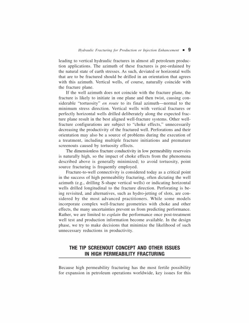
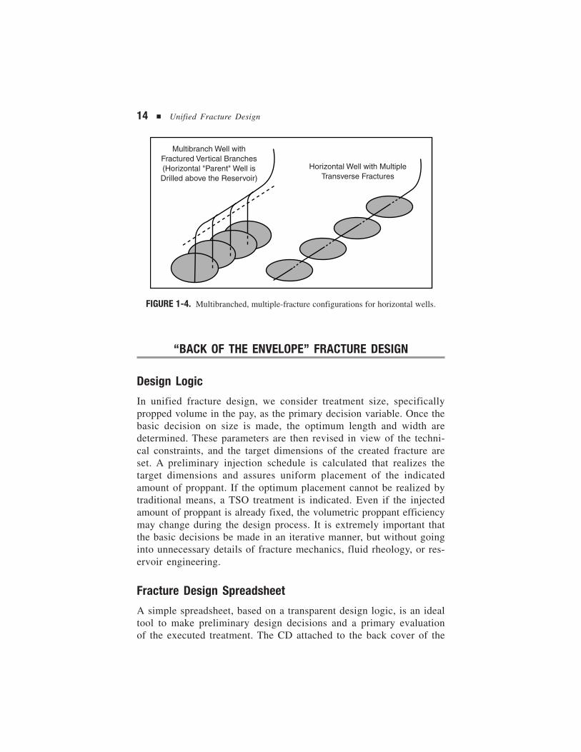
Figure 1-4 illustrates two multi-fracture configurations. A rathersophisticated conceptual configuration would involve the combinationof HPF with multiple-fractured vertical branches emanating from ahorizontal “mother” well drilled above the producing formation. Ofcourse, horizontal wells, being normal to the vertical stress, are gen-erally more prone to wellbore stability problems. Such a configura-tion would allow for placement of the horizontal borehole in acompetent, non-producing interval. There are other advantages to frac-ture treating a vertical section over a highly deviated or horizontalsection: multiple starter fractures, fracture turning, and tortuosity prob-lems are avoided; convergence-flow skins (choke effects) are much lessof a concern; and the perforating strategy is simplified.
FIGURE 1-3. Single-fracture configurations for vertical and horizontal wells.
14 ■ Unified Fracture Design
FIGURE 1-4. Multibranched, multiple-fracture configurations for horizontal wells.
“BACK OF THE ENVELOPE” FRACTURE DESIGN
Design Logic
In unified fracture design, we consider treatment size, specificallypropped volume in the pay, as the primary decision variable. Once thebasic decision on size is made, the optimum length and width aredetermined. These parameters are then revised in view of the techni-cal constraints, and the target dimensions of the created fracture areset. A preliminary injection schedule is calculated that realizes thetarget dimensions and assures uniform placement of the indicatedamount of proppant. If the optimum placement cannot be realized bytraditional means, a TSO treatment is indicated. Even if the injectedamount of proppant is already fixed, the volumetric proppant efficiencymay change during the design process. It is extremely important thatthe basic decisions be made in an iterative manner, but without goinginto unnecessary details of fracture mechanics, fluid rheology, or res-ervoir engineering.
Fracture Design Spreadsheet
A simple spreadsheet, based on a transparent design logic, is an idealtool to make preliminary design decisions and a primary evaluationof the executed treatment. The CD attached to the back cover of the
Multibranch Well withFractured Vertical Branches(Horizontal "Parent" Well isDrilled above the Reservoir)
Horizontal Well with MultipleTransverse Fractures
Hydraulic Fracturing for Production or Injection Enhancement ■ 15
book contains such a spreadsheet, named HF2D. The HF2D Excelspreadsheet is a fast 2D software package for the design of traditional(moderate permeability and hard rock) and frac & pack (higher per-meability and soft rock) fracture treatments.
Readers are strongly encouraged to use the spreadsheet while read-ing the book. By modifying various input parameters, an intuitive feelfor their relative importance in treatment design and final fracturedwell performance can be rapidly acquired, an important but uncom-mon prospect in the era of complex 3D fracture simulators. Thespreadsheet will help readers make the most important decisions andbe aware of their consequences.
The attached spreadsheet is not necessarily intended as a substi-tute for more sophisticated software tools, but the rapid “back of theenvelope” calculations that it affords can provide substantive fracturedesigns. In many cases, by virtue of restricting the analysis to impor-tant first-order considerations, the spreadsheet results are more robustthan those provided by highly involved 3D fracture simulators. It issuggested that readers run parallel cases with one or more 3D simu-lators, if available, as an interesting exercise.

How To Use This Book2
17
The purpose of this book is to transfer hydraulic fracturing technol-ogy and, especially, facilitate its execution. The various chapters sup-ply information on candidate recognition, fracture treatment design,execution and evaluation, materials selection, quality control, andequipment specifications.
While the book includes late developments from some of the mostrespected practitioners of hydraulic fracturing in the world—genuinestate-of-the-art technology—the entry point is deliberately low. Thatis, the book can also serve as a very useful primer for those beingexposed to fracturing technology for the first time.
STRUCTURE OF THE BOOK
Chapters 1 through 10 provide a detailed narrative of the most im-portant aspects across the spectrum of hydraulic fracturing activities.
Appendices A through G are reference material, including a glos-sary of fracturing terms; an extensive bibliography; data requirementsand user instructions for the included design software; standard qual-ity control practices and forms; and example fracturing procedures.
18 ■ Unified Fracture Design
The CD attached to the back cover of the book contains twospreadsheets:
1. The HF2D Excel spreadsheet is a fast 2D software package forthe design of traditional (moderate permeability and hard rock)and frac & pack (higher permeability and soft rock) fracturetreatments.
2. The MF Excel spreadsheet is a minifrac (calibration test) evalu-ation package. Its main purpose is to extract the leakoff coef-ficient from pressure fall-off data.
Two industry-leading references are strongly recommended as addendato this book:
■ Hydraulic Fracture Mechanics, by Peter Valkó and MichaelEconomides, addresses the theoretical background of this semi-nal technology. It provides a fundamental treatment of basicphenomena such as elasticity, stress distribution, fluid flow, andthe dynamics of the rupture process. Contemporary design andanalysis techniques are derived and improved using a compre-hensive and unified approach.
■ Stimulation Engineering Handbook, by John Ely, aptly coversmany issues of fracture treatment implementation and qualitycontrol. This is a very hands-on book, intended to drive execu-tion performance and quality control.
Other reference books that contain abundant information by dozensof experts in the field include Petroleum Well Construction, edited byMichael Economides, Larry Watters, and Shari Dunn-Norman; Reser-voir Stimulation, Third Edition, by Michael Economides and KenNolte; and the somewhat dated but classic volume, SPE MonographNo. 12: Advances in Hydraulic Fracturing, edited by John Gidley,Steve Holditch, Dale Nierode, and Ralph Veatch. While these booksprovide historical perspective as well as in-depth discussion and opin-ions (some controversial) on various details of the fracturing process,they are not recommended for a first reading because of the highlytechnical language and compartmentalized style of presentation.
WHICH SECTIONS ARE FOR YOU
Which sections of the book that you will use—whether it’s a quickreview of the introductory material or a check of the glossary, reading
Hydraulic Fracturing for Production or Injection Enhancement ■ 19
the chapter on fracturing fluids, only, or hands-on use of thedesign theory and software—depends on your role in the fractur-ing operation.
Neither this book nor any other technology transfer mechanism isuseful apart from capable people. The following key personnel com-prise the fracturing team and the targeted readership of this book.
Fracturing Crew
A fracturing crew is the absolute minimum and basic unit required fora fracturing treatment. The crew may consist of anywhere from 7 to15 people, depending on the number of pumping units and the moni-toring capability on location. Many of these people are trained to domultiple jobs, such as driving trucks, hooking up equipment, andinstalling and maintaining the monitoring instruments.
In addition to being trained on each piece of equipment that theywill operate, each member of the fracturing crew should be conver-sant with the material in Chapter 10, On-Site Quality Control, and theaccompanying Appendix F, Standard Practices and QC Forms.
The key people in any fracturing operation, in order of criticalimportance, are:
Frac-Crew Chief—Sometimes known as the field engineer, this is theperson responsible on-site for proper execution of the job. He is ahighly experienced person, either an engineer that has reverted into afield service manager position, or a highly gifted operator who hasbeen promoted to the job. The crew chief directs fracturing operationsfrom the monitoring van (“frac van”) and has complete responsibilityfor the operation, including safety. He communicates constantly bytwo-way radio with all pumping, blender, and proppant storage operators.He is certified to operate high pressure equipment. He understands thefracture design and is responsible for its implementation. He has com-plete authority to continue or shut down a job. (Note that while thepronoun “he” is used for clarity, there are several highly capablewomen currently practicing as fracturing engineers.)
This is not a job that can be learned gradually in a start-up oper-ation. This individual must be identified through a careful searchamong qualified candidates. Extensive and relevant hands-on experiencein fracture execution is a must. The frac-crew chief should be highlyconversant with Unified Fracture Design in its entirety.
Desk Engineer—The desk engineer concept is practiced by many com-panies, within and external to the petroleum industry. Simply put, the
20 ■ Unified Fracture Design
fracturing service company places one of its full-time staff per-manently on location in each client producing company. The client isresponsible to furnish a space (desk) at which the external employee(engineer) can sit and work, giving rise to the term desk engineer. Thisconstant accessibility and the cross-pollination of needs (producingcompany) and capabilities (service company) can dramatically improvethe range and success of application of a technology, and could beespecially important for the rapid and necessarily massive introduc-tion of hydraulic fracturing in a new operating area or country.
This individual will have the same aptitude as the frac-crew chief,but typically with somewhat less experience. Like the frac-crew chief,the desk engineer should become highly conversant with the entirefracturing book.
QA/QC Chemist—Any fracturing operation requires a chemist who iswell versed in the chemistry and physics (rheology) of fracturing fluidsand additives. This person operates a specially outfitted laboratory. Thelaboratory includes, in addition to all basic implements and workingspaces (e.g., hoods), a Fann 50 high-pressure/high-temperature viscom-eter and possibly a fluid shear-history simulator. The chemist shouldhave a background in polymer chemistry, or at least a good under-standing of the subject matter, and should be trained in detecting thequality of proppant (visually, with a 100-magnification microscope).
The chemist is the field quality assurance/quality control (QA/QC)officer. Prior to the fracture treatment, he inspects the make-upwater, fluid additives, and proppant to ensure that they are appropri-ate and that they are of high quality. During the treatment, he makessure that the fracturing materials are blended in the correct propor-tions and at the proper time (e.g., in the case of delayed crosslinkers).He continues to spot check and approve the proppant quality in real-time for the duration of the treatment.
It is almost entirely the responsibility of the QC/QA chemist tounderstand Chapter 6 and Chapter 9 of this book, as well as Appen-dix F, and to revise them for company-specific needs. In addition, thisperson should fully digest the Stimulation Engineering Handbook.
Fracture Design Engineer—As the title suggests, this individual isresponsible for design of the fracturing treatment. The fracture designengineer must master the basics of hydraulic fracturing, as included inChapters 4 through 9, and should be proficient to run the includedfracture design software. Depending on the magnitude of the fracturingactivity, there could be several people trained to perform this task. In
Hydraulic Fracturing for Production or Injection Enhancement ■ 21
small operations, the same person may double-up as the field engi-neer that performs real-time analysis of the treatment from the fracvan (Chapter 10).
The fracture design engineer must have an engineering background,preferably petroleum engineering, and be dedicated to study the subtleand sometimes complex aspects of fracture design. Experience in theindustry is desirable, but not necessary. With proper training, a giftedperson can start functioning properly after several jobs. Ultimately, thefracturing engineer should be broadly conversant in fracture execution,fracturing fluid chemistry, and well completions. He should be ableto make critical use of the additional literature recommended above.

Well Stimulation as aMeans to Increase theProductivity Index3
23
The primary goal of well stimulation is to increase the productivityof a well by removing damage in the vicinity of the wellbore or bysuperimposing a highly conductive structure onto the formation. Com-monly used stimulation techniques include hydraulic fracturing, frac& pack, carbonate and sandstone matrix acidizing, and fractureacidizing. Any of these stimulation techniques can be expected togenerate some increase in the productivity index, which, in turn, canbe used either to increase the production rate or decrease the pres-sure drawdown. There is no need to explain the benefits of increas-ing the production rate. The benefits of decreased pressure drawdownare less obvious, but include minimizing sand production and waterconing and/or shifting the phase equilibrium in the near-well zone toreduce condensate formation. Injection wells also benefit from stimu-lation in a similar manner.
To understand how stimulation increases productivity, basic pro-duction and reservoir engineering concepts are presented below.
PRODUCTIVITY INDEX
In discussing the productivity of a specific well, we think of a linearrelation between the production rate and the driving force (pres-sure drawdown),
24 ■ Unified Fracture Design
q J p= ∆ (3-1)
where the proportionality “constant” J is called the productivityindex (PI). During its lifespan, a well is subject to several changes inflow conditions, but the two most important idealizations are constantproduction rate,
∆pBq
khpD= α µ
π1
2(3-2)
and constant drawdown pressure,
qkh pB
qD= 2
1
πα µ
∆(3-3)
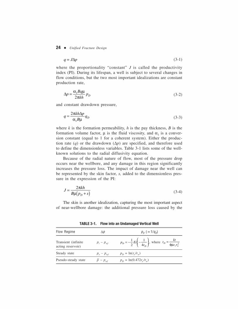
where k is the formation permeability, h is the pay thickness, B is theformation volume factor, µ is the fluid viscosity, and α1 is a conver-sion constant (equal to 1 for a coherent system). Either the produc-tion rate (q) or the drawdown (∆p) are specified, and therefore usedto define the dimensionless variables. Table 3-1 lists some of the well-known solutions to the radial diffusivity equation.
Because of the radial nature of flow, most of the pressure dropoccurs near the wellbore, and any damage in this region significantlyincreases the pressure loss. The impact of damage near the well canbe represented by the skin factor, s, added to the dimensionless pres-sure in the expression of the PI:
Jkh
B p sD
=+( )
2πµ (3-4)
The skin is another idealization, capturing the most important aspectof near-wellbore damage: the additional pressure loss caused by the
TABLE 3-1. Flow into an Undamaged Vertical Well
Flow Regime ∆p pD (G1/qD)
Transient (infinite pi – pwf p EitD
D
= − −
12
14
, where tktc rD
t w
=φµ 2
acting reservoir)
Steady state pe – pwf pD = ln(re /rw)
Pseudo-steady state p– – pwf pD = ln(0.472re /rw)

Well Stimulation as a Means to Increase the Productivity Index ■ 25
damage is proportional to the production rate. Even with best drillingand completion practices, some kind of near-well damage is presentin most cases. The skin can be considered as the measure of the “good-ness” of a well. Other mechanical factors, not caused by damage perse may add to the skin effect. These may include bad perforations,partial well penetration, or undersized well completion equipment, andso on. If the well is damaged (or its productivity is less than the idealreference value for any other reason), the skin factor is positive.
Well stimulation increases the productivity index. It is reasonableto look at any type of stimulation as an operation to reduce the skinfactor. With the generalization to negative values of skin factor, evensuch stimulation treatments—which not only remove damage but alsosuperimpose some new or improved conductivity paths—can be putinto this framework. In the latter case, it is more correct to speak aboutpseudo-skin factor, indicating that stimulation causes some structuralchanges in the fluid flow path as well as removing damage.
As we explained in Chapter 1, crucial from the fracture designviewpoint is the pseudo-steady state productivity index:
Jq
p pkhB
Jwf
D=−
= 2
1
πα µ (3-5)
where JD is called the dimensionless productivity index.For a well located in the center of a circular drainage area, the
dimensionless productivity index in pseudo-steady state reduces to
Jr
rs
De
w
=
+
1
0 472ln
. (3-6)
In the case of a propped fracture, there are several ways to incor-porate the stimulation effect into the productivity index. One can usethe pseudo-skin concept,
Jr
rs
De
wf
=
+
1
0 472ln
. (3-7)
or the equivalent wellbore radius concept,
Jr
r
De
w
=
′
1
0 472ln
. (3-8)
26 ■ Unified Fracture Design
or one can just provide the dimensionless productivity index as a func-tion of the fracture parameters,
JD
= function of drainage-volume geometryand fracture parameters (3-9)
All three options give exactly the same results (if done in coher-ent terms). The last option is the most general and convenient, espe-cially if we wish to consider fractured wells in more general drainageareas (not necessarily circular).
Many authors have provided charts and correlations in one formor another to handle special geometries and reservoir types. Unfortunately,most of the results are less obvious or difficult to apply in higherpermeability cases. Even for the simplest possible case, a vertical frac-ture intersecting a vertical well, there are quite large discrepancies (see,for instance, Figure 12-13 of Reservoir Stimulation, Third Edition).
THE WELL-FRACTURE-RESERVOIR SYSTEM
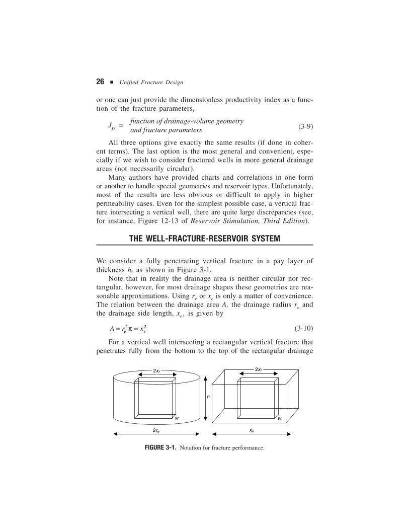
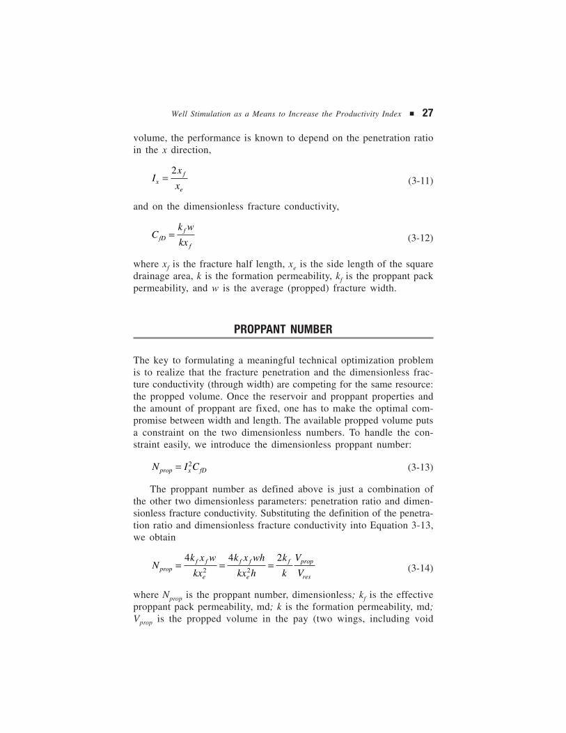
We consider a fully penetrating vertical fracture in a pay layer ofthickness h, as shown in Figure 3-1.
Note that in reality the drainage area is neither circular nor rec-tangular, however, for most drainage shapes these geometries are rea-sonable approximations. Using re or xe is only a matter of convenience.The relation between the drainage area A, the drainage radius re andthe drainage side length, xe , is given by
A r xe e= =2 2π (3-10)
For a vertical well intersecting a rectangular vertical fracture thatpenetrates fully from the bottom to the top of the rectangular drainage
FIGURE 3-1. Notation for fracture performance.
h
2re xe
w
2xf2xf
w
Well Stimulation as a Means to Increase the Productivity Index ■ 27
volume, the performance is known to depend on the penetration ratioin the x direction,
Ix
xxf
e
=2
(3-11)
and on the dimensionless fracture conductivity,
Ck w
kxfDf
f
= (3-12)
where xf is the fracture half length, xe is the side length of the squaredrainage area, k is the formation permeability, kf is the proppant packpermeability, and w is the average (propped) fracture width.
PROPPANT NUMBER
The key to formulating a meaningful technical optimization problemis to realize that the fracture penetration and the dimensionless frac-ture conductivity (through width) are competing for the same resource:the propped volume. Once the reservoir and proppant properties andthe amount of proppant are fixed, one has to make the optimal com-promise between width and length. The available propped volume putsa constraint on the two dimensionless numbers. To handle the con-straint easily, we introduce the dimensionless proppant number:
N I Cprop x fD= 2 (3-13)
The proppant number as defined above is just a combination ofthe other two dimensionless parameters: penetration ratio and dimen-sionless fracture conductivity. Substituting the definition of the penetra-tion ratio and dimensionless fracture conductivity into Equation 3-13,we obtain
Nk x w
kx
k x wh
kx h
k
k
V
Vpropf f
e
f f
e
f prop
res
= = =4 4 2
2 2 (3-14)
where Nprop is the proppant number, dimensionless; kf is the effectiveproppant pack permeability, md; k is the formation permeability, md;Vprop is the propped volume in the pay (two wings, including void
28 ■ Unified Fracture Design
space between the proppant grains), ft3; and Vres is the drainage vol-ume (i.e., drainage area multiplied by pay thickness), ft3. (Of course,any other coherent units can be used, because the proppant numberinvolves only the ratio of permeabilities and the ratio of volumes.)
Equation 3-14 plainly reveals the meaning of the proppant num-ber: it is the weighted ratio of propped fracture volume (two wings)to reservoir volume, with a weighting factor of two times the proppant-to-formation permeability contrast. Notice, only the proppant thatreaches the pay layer is counted in the propped volume. If, forinstance, the fracture height is three times the net pay thickness, thenVprop can be estimated as the bulk (packed) volume of injectedproppant divided by three. In other words, the packed volume of theinjected proppant multiplied by the volumetric proppant efficiencyyields the Vprop used in calculating the proppant number.
The dimensionless proppant number, Nprop , is by far the mostimportant parameter in unified fracture design.
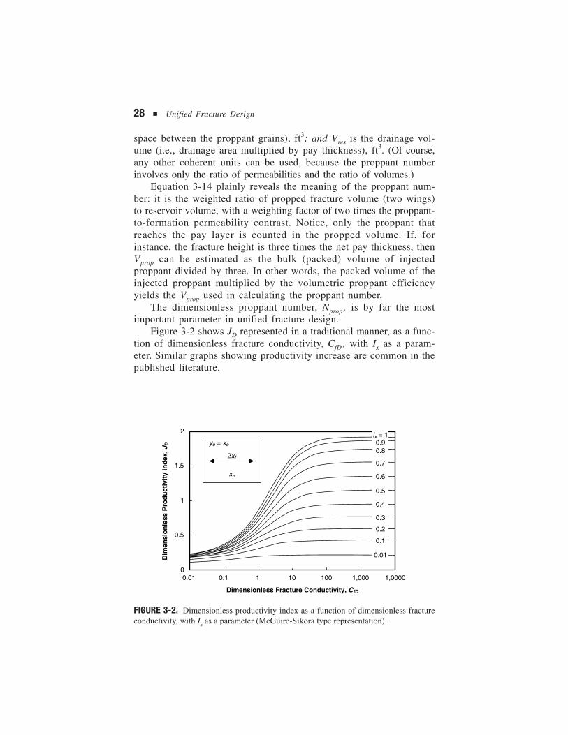
Figure 3-2 shows JD represented in a traditional manner, as a func-tion of dimensionless fracture conductivity, CfD , with Ix as a param-eter. Similar graphs showing productivity increase are common in thepublished literature.
FIGURE 3-2. Dimensionless productivity index as a function of dimensionless fractureconductivity, with I
x as a parameter (McGuire-Sikora type representation).
0
0.5
1
1.5
2
0.01 0.1 1 10 100 1,000 1,0000
Dimensionless Fracture Conductivity, CfD
Dim
ensi
on
less
Pro
du
ctiv
ity
Ind
ex, J
D
xe
2xf
ye = xe
lx = 10.90.8
0.7
0.6
0.5
0.4
0.3
0.2
0.1
0.01
Well Stimulation as a Means to Increase the Productivity Index ■ 29
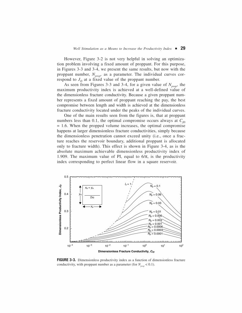
However, Figure 3-2 is not very helpful in solving an optimiza-tion problem involving a fixed amount of proppant. For this purpose,in Figures 3-3 and 3-4, we present the same results, but now with theproppant number, Nprop, as a parameter. The individual curves cor-respond to JD at a fixed value of the proppant number.
As seen from Figures 3-3 and 3-4, for a given value of Nprop, themaximum productivity index is achieved at a well-defined value ofthe dimensionless fracture conductivity. Because a given proppant num-ber represents a fixed amount of proppant reaching the pay, the bestcompromise between length and width is achieved at the dimensionlessfracture conductivity located under the peaks of the individual curves.
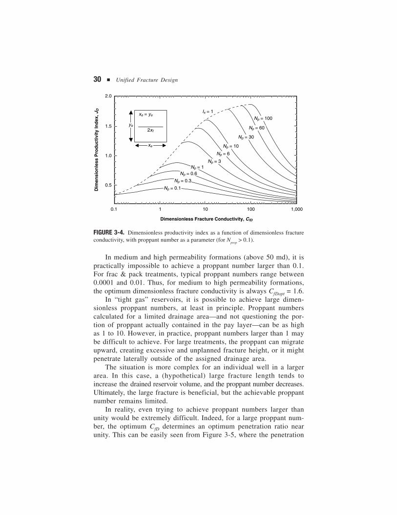
One of the main results seen from the figures is, that at proppantnumbers less than 0.1, the optimal compromise occurs always at CfD
= 1.6. When the propped volume increases, the optimal compromisehappens at larger dimensionless fracture conductivities, simply becausethe dimensionless penetration cannot exceed unity (i.e., once a frac-ture reaches the reservoir boundary, additional proppant is allocatedonly to fracture width). This effect is shown in Figure 3-4, as is theabsolute maximum achievable dimensionless productivity index of1.909. The maximum value of PI, equal to 6/π, is the productivityindex corresponding to perfect linear flow in a square reservoir.
FIGURE 3-3. Dimensionless productivity index as a function of dimensionless fractureconductivity, with proppant number as a parameter (for N
prop < 0.1).
0.5
0.4
0.3
0.2
10–4
Dimensionless Fracture Conductivity, CfD
Dim
ensi
on
less
Pro
du
ctiv
ity
Ind
ex, J
D
10–3 10–2 10–1 100 101 102
Np = 0.1
Np = 0.06
Np = 0.03
Np = 0.01Np = 0.006
Np = 0.003Np = 0.001
Np = 0.0006Np = 0.0003Np = 0.0001
2xf
xe = ye
xe
ye
lx = 1
30 ■ Unified Fracture Design
In medium and high permeability formations (above 50 md), it ispractically impossible to achieve a proppant number larger than 0.1.For frac & pack treatments, typical proppant numbers range between0.0001 and 0.01. Thus, for medium to high permeability formations,the optimum dimensionless fracture conductivity is always CfDopt = 1.6.
In “tight gas” reservoirs, it is possible to achieve large dimen-sionless proppant numbers, at least in principle. Proppant numberscalculated for a limited drainage area—and not questioning the por-tion of proppant actually contained in the pay layer—can be as highas 1 to 10. However, in practice, proppant numbers larger than 1 maybe difficult to achieve. For large treatments, the proppant can migrateupward, creating excessive and unplanned fracture height, or it mightpenetrate laterally outside of the assigned drainage area.
The situation is more complex for an individual well in a largerarea. In this case, a (hypothetical) large fracture length tends toincrease the drained reservoir volume, and the proppant number decreases.Ultimately, the large fracture is beneficial, but the achievable proppantnumber remains limited.
In reality, even trying to achieve proppant numbers larger thanunity would be extremely difficult. Indeed, for a large proppant num-ber, the optimum CfD determines an optimum penetration ratio nearunity. This can be easily seen from Figure 3-5, where the penetration
FIGURE 3-4. Dimensionless productivity index as a function of dimensionless fractureconductivity, with proppant number as a parameter (for N
prop > 0.1).
2.0
1.5
1.0
0.5
0.1 1 10 100 1,000
Dimensionless Fracture Conductivity, CfD
Dim
ensi
on
less
Pro
du
ctiv
ity
Ind
ex, J
D
2xf
xe = ye
xe
ye
Np = 100
Np = 60
Np = 30
Np = 10
Np = 6
Np = 3Np = 1
Np = 0.6
Np = 0.3
Np = 0.1
Ix = 1
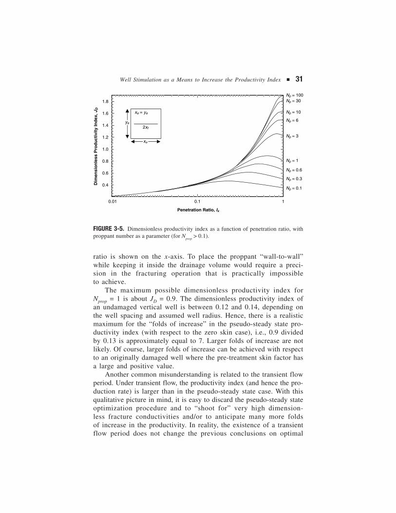
Well Stimulation as a Means to Increase the Productivity Index ■ 31
ratio is shown on the x-axis. To place the proppant “wall-to-wall”while keeping it inside the drainage volume would require a preci-sion in the fracturing operation that is practically impossibleto achieve.
The maximum possible dimensionless productivity index forNprop = 1 is about JD = 0.9. The dimensionless productivity index ofan undamaged vertical well is between 0.12 and 0.14, depending onthe well spacing and assumed well radius. Hence, there is a realisticmaximum for the “folds of increase” in the pseudo-steady state pro-ductivity index (with respect to the zero skin case), i.e., 0.9 dividedby 0.13 is approximately equal to 7. Larger folds of increase are notlikely. Of course, larger folds of increase can be achieved with respectto an originally damaged well where the pre-treatment skin factor hasa large and positive value.
Another common misunderstanding is related to the transient flowperiod. Under transient flow, the productivity index (and hence the pro-duction rate) is larger than in the pseudo-steady state case. With thisqualitative picture in mind, it is easy to discard the pseudo-steady stateoptimization procedure and to “shoot for” very high dimension-less fracture conductivities and/or to anticipate many more foldsof increase in the productivity. In reality, the existence of a transientflow period does not change the previous conclusions on optimal
FIGURE 3-5. Dimensionless productivity index as a function of penetration ratio, withproppant number as a parameter (for N
prop > 0.1).
1.8
1.6
1.4
1.2
1.0
0.8
0.6
0.4
0.01 0.1 1
Penetration Ratio, Ix
Dim
ensi
on
less
Pro
du
ctiv
ity
Ind
ex, J
D
2xf
xe = ye
xe
ye
Np = 100Np = 30
Np = 10
Np = 6
Np = 3
Np = 1
Np = 0.6
Np = 0.3
Np = 0.1
32 ■ Unified Fracture Design
dimensions. Our calculations show that there is no reason to departfrom the optimum compromise derived for the pseudo-steady statecase, even if the well will produce in the transient regime for a con-siderable time (say months or even years). Simply stated, what is goodfor maximizing pseudo-steady state flow is also good for maximizingtransient flow.
In the definition of proppant number, kf is the effective (or equiva-lent, as it is sometimes called) permeability of the proppant pack. Thisparameter is crucial in design. Current fracture simulators generallyprovide a nominal value for the proppant pack permeability (suppliedby the proppant manufacturer) and allow it to be reduced by a factorthat the user selects. The already-reduced value should be used in theproppant number calculation.
There are numerous reasons why the actual (or equivalent) proppantpack permeability will be lower than the nominal value. The mainreasons are as follows:
■ Large closure stresses crush the proppant, reducing the averagegrain size, grain uniformity, and porosity.
■ Fracturing fluid residue decreases the permeability in the fracture.
■ High fluid velocity in the proppant pack creates “non-Darcyeffects,” resulting in additional pressure loss. This phenomenoncan be significant when gas is produced in the presence of aliquid (water and/or condensate). The non-Darcy effect is causedby the periodic acceleration-deceleration of the liquid droplets,effectively reducing the permeability of the proppant pack. Thisreduced permeability can be an order of magnitude lower thanthe nominal value presented by the manufacturer.
During the fracture design, considerable attention must be paid tothe effective permeability of the proppant pack and to the permeabil-ity of the formation. Knowledge of the effective permeability contrastis crucial, and cannot be substituted by qualitative reasoning.
Well Performance for Lowand Moderate Proppant Numbers
By low and moderate proppant numbers, we mean anything lessthan 0.1. The most dynamic fracturing activities (frac & pack, forexample) fall into this category—making it extremely important froma design standpoint.
Well Stimulation as a Means to Increase the Productivity Index ■ 33
The optimum treatment design for moderate proppant numbers canbe simply and concisely presented in an analytical form. In the process,we will show how the proppant number and dimensionless produc-tivity index relate to some other popular performance indicators, suchas the Cinco-Ley and Samaniego pseudo-skin function and Prats’equivalent wellbore radius. In fact, fracture designs based on theserelated performance indicators are just the moderate (low) proppantnumber limit of the more comprehensive unified fracture design.
Prats (1961) introduced the concept of equivalent wellbore radiusresulting from a fracture treatment. He also showed that, except forthe fracture extent, all fracture variables affect well performance onlythrough the combined quantity of dimensionless fracture conductiv-ity. When the dimensionless fracture conductivity is high (e.g., greaterthan 100), the behavior is similar to that of an infinite conductivityfracture. The behavior of infinite conductivity fractures was studiedlater by Gringarten and Ramey (1974). To characterize the impact ofa finite-conductivity vertical fracture on the performance of a verticalwell, Cinco-Ley and Samaniego (1981) introduced a pseudo-skin func-tion which is strictly a function of dimensionless fracture conductivity.
According to the definition of pseudo-skin factor, the dimen-sionless pseudo-steady state productivity index can be given as
J r
rs
De
wf
=+
1
0 472ln . (3-15)
where sf is the pseudo-skin. In Prats’ notation the same productivityindex is described by
J r
r
De
w
=
′
1
0 472ln .(3-16)
where ′rw is the equivalent wellbore radius. Prats also used the rela-tive equivalent wellbore radius defined by ′r xw f/ .
In the Cinco-Ley formalism, the productivity index is described as
J r
xf
De
f
=+
1
0 472ln .(3-17)
where f is the pseudo-skin function with respect to the fracture half-length.
34 ■ Unified Fracture Design
Table 3-2 shows the relations between these quantities.The advantage of the Cinco-Ley and Samaniego formalism ( f-factor)
is that, for moderate (and low) proppant numbers, the quantity fdepends only on the dimensionless fracture conductivity. The solid linein Figure 3-6 shows the Cinco-Ley and Samaniego f-factor as a func-tion of dimensionless fracture conductivity.
Note that for large values of CfD, the f-factor expression approachesln(2), indicating that the production from an infinite conductivity frac-ture is equivalent to the production of π/2 times more than the pro-duction from the same surface arranged cylindrically (like the wall ofa huge wellbore). In calculations, it is convenient to use an explicitexpression of the form
f. . u . u. u . u . u
u CfD= − ++ + +
=165 0 328 01161 018 0 064 0 005
2
2 3, ln where (3-18)
Because the relative wellbore radius of Prats can be also expressedby the f-factor (see Table 3-2), we obtain the equivalent result:
′ = − − ++ + +
=r
x. . u . u. u . u . u
u Cw
ffDexp , ln
165 0 328 01161 018 0 064 0 005
2
2 3 where (3-19)
The simple curve-fits represented by Equations 3-18 and 3-19 areonly valid over the range indicated in Figure 3-6. For very large val-ues of CfD, one can simply use the limiting value for Equation 3-19,which is 0.5, showing that the infinite conductivity fracture has aproductivity similar to an imaginary (huge) wellbore with radius xf /2.
Interestingly enough, infinite conductivity behavior does not meanthat we have selected the optimum way to place a given amount ofproppant into the formation.
TABLE 3-2. Relations Between Various Performance Indicators
f sx
rff
w
= +
ln s
r
rfw
w
=′
ln
′ = −r r sw w fexp[ ] ′ = −r x fw f exp[ ]
′ = −r
xfw
f
exp[ ]′ = −r
x
r
xsw
f
w
ffexp[ ]
Well Stimulation as a Means to Increase the Productivity Index ■ 35
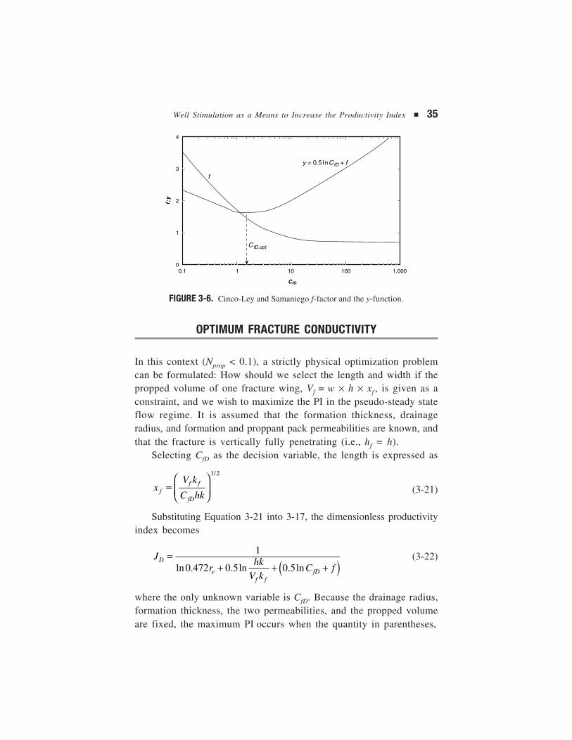
FIGURE 3-6. Cinco-Ley and Samaniego f-factor and the y-function.
OPTIMUM FRACTURE CONDUCTIVITY
In this context (Nprop < 0.1), a strictly physical optimization problemcan be formulated: How should we select the length and width if thepropped volume of one fracture wing, Vf = w × h × xf , is given as aconstraint, and we wish to maximize the PI in the pseudo-steady stateflow regime. It is assumed that the formation thickness, drainageradius, and formation and proppant pack permeabilities are known, andthat the fracture is vertically fully penetrating (i.e., hf = h).
Selecting CfD as the decision variable, the length is expressed as
xV k
C hkff f
fD
=
1 2/
(3-21)
Substituting Equation 3-21 into 3-17, the dimensionless productivityindex becomes
Jr
hkV k
C fD
ef f
fD
=+ + +( )
1
0 472 0 5 0 5ln . . ln . ln(3-22)
where the only unknown variable is CfD. Because the drainage radius,formation thickness, the two permeabilities, and the propped volumeare fixed, the maximum PI occurs when the quantity in parentheses,
4
3
2
1
00.1 1 10 100 1,000
CfD
f;y
y = 0.5lnCfD + f
CfD,opt
f
36 ■ Unified Fracture Design
y C ffD= +0 5. ln (3-23)
reaches a minimum. That quantity is also shown in Figure 3-6. Becausethe above expression depends only on CfD, the optimum, CfD,opt = 1.6is a given constant for any reservoir, well, and proppant volume.
This result provides a deeper insight to the real meaning ofdimensionless fracture conductivity. The reservoir and the fracture canbe considered as a system working in series. The reservoir can feedmore fluids into the fracture if the length is larger, but (since thevolume is fixed) this means a narrower fracture. In a narrow fracture,the resistance to flow may be significant. The optimum dimension-less fracture conductivity corresponds to the best compromise betweenthe requirements of the two subsystems. Once it is found, the optimumfracture half-length can be calculated from the definition of CfD as
xV k
hkff f=
1 6
1 2
.
/
(3-24)
and consequently, the optimum propped average width should be
wV k
hk
V
hxf
f
f
f
=
=
1 61 2
./
(3-25)
Notice that Vf is Vprop/2 because it is only one half of the proppedvolume.
The most important implication of the above results is that thereis no theoretical difference between low and high permeability frac-turing. In all cases, there exists a physically optimal fracture thatshould have a CfD near unity. In low permeability formations, thisrequirement results in a long and narrow fracture; in high permeabil-ity formations, a short and wide fracture provides the same dimen-sionless conductivity.
If the fracture length and width are selected according to theoptimum compromise, the dimensionless productivity index will be
JND
prop,max . . ln
=−
10 99 0 5
(3-26)
Of course, the indicated optimal fracture dimensions may not betechnically or economically feasible. In low permeability formations,
Well Stimulation as a Means to Increase the Productivity Index ■ 37
the indicated fracture length may be too large, or the extreme narrowwidth may mean that the assumed constant proppant permeability isno longer valid. In high permeability formations, the indicated largewidth might be impossible to create. For more detailed calculations,all the constraints must be taken into account, but, in any case, adimensionless fracture conductivity far from the optimum indicates thateither the fracture is a relative “bottleneck” (CfD << 1.6) or that it istoo “short and wide” (CfD >> 1.6).
The reader should not forget that the results of this section—including the Cinco-Ley and Samaniego graph and its curve fit, theoptimum dimensionless fracture conductivity of 1.6, and Equation 3-26—are valid only for proppant numbers less than 0.1. This can be easilyseen by comparing Figures 3-3 and 3-4. In Figure 3-3, the curves havetheir maximum at CfD = 1.6, and the maximum JD corresponds to thesimple Equation 3-26. In Figure 3-4, however, where the proppantnumbers are larger than 0.1, the location of the maximum is shifted,and the simple calculations based on the f-factor (Equation 3-18) oron the equivalent wellbore radius (Equation 3-19) are no longer valid.
Optimization routines found on the CD that accompanies this bookare based on the full information contained in Figures 3-3 and 3-4,and formulas developed for moderate proppant numbers are used onlyin the range of their validity.
DESIGN LOGIC
We wish to place a certain amount of proppant in the pay interval andto place it in such a way that the maximum possible productivityindex is realized. The key to finding the right balance between sizeand productivity improvement is in the proppant number. Since Vprop
includes only that part of the proppant that reaches the pay, and henceis dependent on the volumetric proppant efficiency, the proppant num-ber cannot be simply fixed during the design procedure.
In unified fracture design, we specify the amount of proppantindicated for injection and then proceed as follows:
1. Assume a volumetric proppant efficiency and determine theproppant number. (Once the treatment details are obtained, theassumed volumetric proppant efficiency related to created frac-ture height may be revisited and the design process may berepeated in an iterative manner.)
38 ■ Unified Fracture Design
2. Use Figure 3-3 or Figure 3-4 (or rather the design spreadsheet)to calculate the maximum possible productivity index, JDmax ,and also the optimum dimensionless fracture conductivity,CfDopt , from the proppant number.
3. Calculate the optimum fracture half-length. Denoting the vol-ume of one propped wing (in the pay) by Vf , the optimum frac-ture half-length can be calculated as
xV k
C hkff f
fD opt
=
,
/1 2
(3-27)
4. Calculate the optimum averaged propped fracture width as
wC V k
hk
V
x hfD opt f
f
f
f
=
=,
/1 2
(3-28)
In the above two equations, Vf and h must correspond to eachother. If total fracture height is used for h, which is often denoted byhf , then the proppant volume Vf must be the total propped volume ofone wing. However, if the selected Vf corresponds only to that por-tion of one wing volume that is contained in the pay layer, then hshould be the net thickness of the pay. The final result for optimumlength and width will be the same in either case. It is a better practice,however, to use net thickness and net volume (contained in the pay)because those variables are also used to calculate the proppant number.
Once reservoir engineering and economic considerations have dic-tated the fracture dimensions to be created, the next issue is how toachieve that goal. From this point, design of the fracture treatment canbe viewed as adjusting treatment details (pumping time and proppantschedule) to achieve the desired final fracture dimensions.
In the next chapter, we outline the mechanics of fracture creationin some detail. This theoretical basis is needed before we can proceedto design the fracture treatment, our ultimate goal.
Fracturing Theory4
39
In the following, we briefly summarize the most important mechani-cal concepts related to hydraulic fracturing.
LINEAR ELASTICITY AND FRACTURE MECHANICS
Elasticity implies reversible changes. The initiation and propagationof a fracture means that the material has responded in an inherentlynon-elastic way, and an irreversible change has occurred. Neverthe-less, linear elasticity is a useful tool when studying fractures becauseboth the stresses and strains (except perhaps in the vicinity of thefracture face, and especially the tip) may still be adequately describedby elasticity theory.
A linear elastic material is characterized by elastic constants thatcan be determined in static or dynamic loading experiments. For anisotropic material, where the properties are independent of direction,two constants are sufficient to describe the behavior.
Figure 4-1 is a schematic representation of a static experiment withuniaxial loading. The two parameters obtained from such an experi-ment are the Young’s modulus (E) and the Poisson ratio (ν). They are
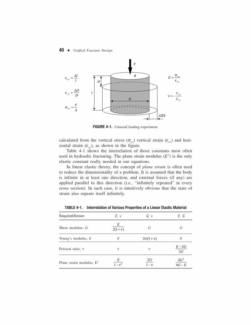
40 ■ Unified Fracture Design
FIGURE 4-1. Uniaxial loading experiment.
calculated from the vertical stress (σxx) vertical strain (εxx) and hori-zontal strain (εyy), as shown in the figure.
Table 4-1 shows the interrelation of those constants most oftenused in hydraulic fracturing. The plane strain modulus (E�) is the onlyelastic constant really needed in our equations.
In linear elastic theory, the concept of plane strain is often usedto reduce the dimensionality of a problem. It is assumed that the bodyis infinite in at least one direction, and external forces (if any) areapplied parallel to this direction (i.e., “infinitely repeated” in everycross section). In such case, it is intuitively obvious that the state ofstrain also repeats itself infinitely.
TABLE 4-1. Interrelation of Various Properties of a Linear Elastic Material
Required/Known E, ν G, ν E, G
Shear modulus, GE
2 1+( )ν G G
Young’s modulus, E E 2 1G +( )ν E
Poisson ratio, ν ν ν E GG
− 22
Plane strain modulus, E�E
1 2− ν2
1G
− ν4
4
2GG E−
ε xxl
l= ∆
ε yyD
D= ∆
σ xxFA
=
E xx
xx
= σε
νεε
= – yy
xx
∆I
I
F
A
D
∆D/2
Fracturing Theory ■ 41
Plane strain is a reasonable approximation in a simplified descrip-tion of hydraulic fracturing. The main question is how to select theplane. Two possibilities arise, and, in turn, this has given rise to twodifferent approaches to fracture modeling. The state of plane strain wasassumed in the horizontal plane by Khristianovitch and Zheltov (1955)and by Geertsma and de Klerk (1969), while plane strain in the ver-tical plane (normal to the direction of fracture propagation) wasassumed by Perkins and Kern (1961) and Nordgren (1972).
Often, in the hydraulic fracturing literature, the term “KGD”geometry is used interchangeably to the horizontal plane-strain assump-tion and “PKN” geometry is used as a substitute for postulating planestrain in the vertical plane.
Exact mathematical solutions are available for the problem of apressurized crack in the state of plane strain. In particular, it is wellknown that the pressurized line crack has an elliptical width distribu-tion (Sneddon, 1973):
w xp
Ec x( ) =
′−4 0 2 2 (4-1)
where x is the distance from the center of the crack, c is the half-length (the distance of the tip from the center) and p0 is the constantpressure exerted on the crack faces from inside. From Equation 4-1,the maximum width at the center is
wcp
E004=
′ (4-2)
indicating that a linear relationship is maintained between the crackopening induced and the pressure exerted. When the concept of pres-surized line crack is applied for a real situation, p0 is substituted withthe net pressure, pn , defined as the difference of the inner pressureand the minimum principal stress acting from outside, trying to closethe fracture (Hubbert and Willis, 1957; Haimson and Fairhurst, 1967).
Fracture mechanics has emerged from the observation that anyexisting discontinuity in a solid deteriorates its ability to carry loads.A (possibly small) hole may give rise to high local stresses comparedto the ones being present without the hole. The high stresses, even ifthey are limited to a small area, may lead to the rupture of the mate-rial. It is often convenient to look at material discontinuities as stressconcentrators which locally increase the otherwise present stresses.
42 ■ Unified Fracture Design
Two main cases must be distinguished. If the form of discontinu-ity is smooth (e.g., a circular borehole in a formation), then the maxi-mum stress around the discontinuity is higher than the virgin stressby a finite factor, which depends on the geometry. For example, thestress concentration factor for a circular borehole is three.
The situation is different in the case of sharp edges, such as atthe tip of a fracture. Then the maximum stress at the tip becomesinfinite. In fracture mechanics, we have to deal with singularities. Twodifferent loadings (pressure distributions) of a line crack result in twodifferent stress distributions. Both cases may yield infinite stresses atthe tip, but the “level of infinity” is different. We need a quantity tocharacterize this difference. Fortunately, all stress distributions nearthe tip of any fracture are similar in the sense that they decreaseaccording to r –1/2, where r is the distance from the tip. The quantityused to characterize the “level of infinity” is the stress intensity fac-tor, KI, defined as the multiplier to the r–1/2 function. For the ideali-zation of a pressurized line crack with half-length, c, and constantpressure, p0, the stress intensity factor is given by
K p cI = 01 2/ (4-3)
In other words, the stress intensity factor at the tip is proportional tothe constant pressure opening up the crack and to the square root ofthe crack half-length (characteristic dimension).
According to the key postulate of linear elastic fracture mechan-ics (LEFM), for a given material there is a critical value of the stressintensity factor, KIC , called fracture toughness. If the stress intensityfactor at the crack tip is above the critical value, the crack will propa-gate; otherwise it will not. Fracture toughness is a useful quantity forsafety calculations, when the engineer’s only concern is to avoid frac-turing. In well stimulation, where the engineer’s primary goal is tocreate and propagate a fracture, the concept has been found some-what controversial because it predicts that less and less effort is nec-essary to propagate a fracture with increasing extent. In the large scale,however, the opposite is usually true.
FRACTURING FLUID MECHANICS
Fluid materials deform continuously (in other words, flow) withoutrupture when subjected to a constant stress. Solids generally will assume
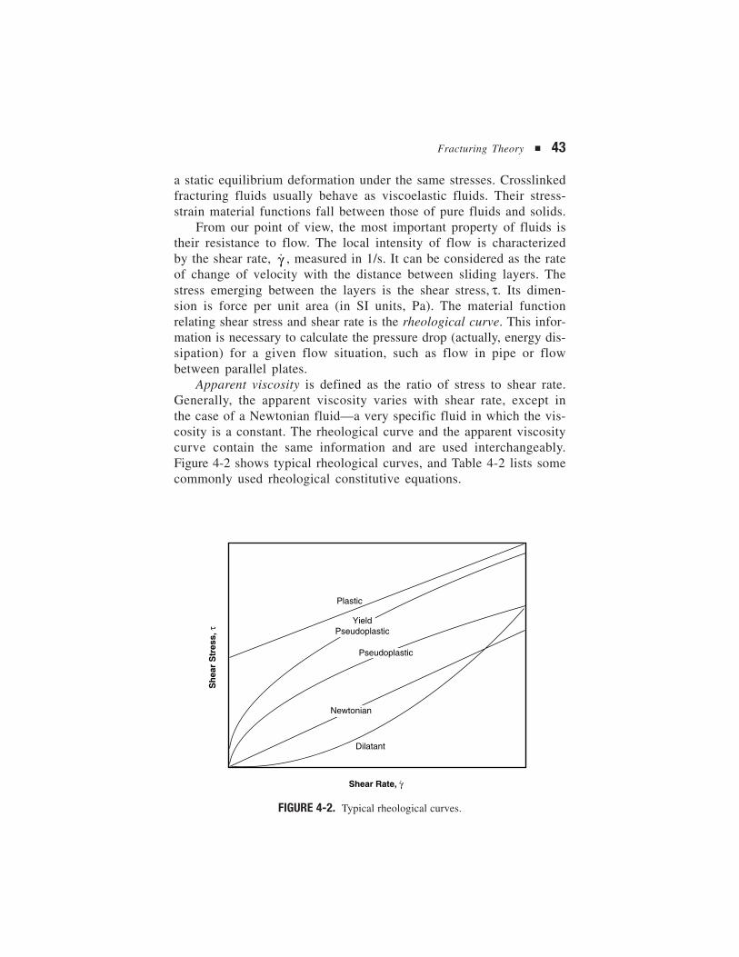
Fracturing Theory ■ 43
a static equilibrium deformation under the same stresses. Crosslinkedfracturing fluids usually behave as viscoelastic fluids. Their stress-strain material functions fall between those of pure fluids and solids.
From our point of view, the most important property of fluids istheir resistance to flow. The local intensity of flow is characterizedby the shear rate, γ̇ , measured in 1/s. It can be considered as the rateof change of velocity with the distance between sliding layers. Thestress emerging between the layers is the shear stress, τ. Its dimen-sion is force per unit area (in SI units, Pa). The material functionrelating shear stress and shear rate is the rheological curve. This infor-mation is necessary to calculate the pressure drop (actually, energy dis-sipation) for a given flow situation, such as flow in pipe or flowbetween parallel plates.
Apparent viscosity is defined as the ratio of stress to shear rate.Generally, the apparent viscosity varies with shear rate, except inthe case of a Newtonian fluid—a very specific fluid in which the vis-cosity is a constant. The rheological curve and the apparent viscositycurve contain the same information and are used interchangeably.Figure 4-2 shows typical rheological curves, and Table 4-2 lists somecommonly used rheological constitutive equations.
FIGURE 4-2. Typical rheological curves.
Plastic
Newtonian
Dilatant
Sh
ear
Str
ess,
τ
Shear Rate, γ̇
YieldPseudoplastic
Pseudoplastic
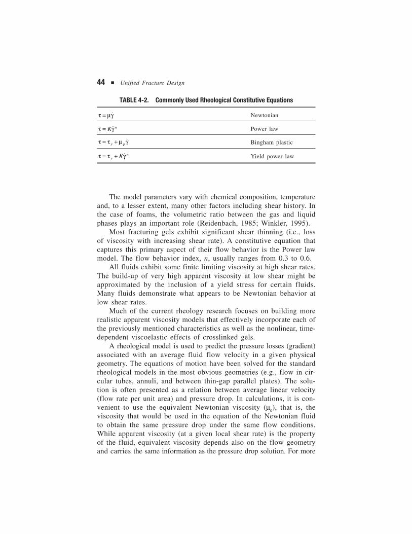
44 ■ Unified Fracture Design
The model parameters vary with chemical composition, temperatureand, to a lesser extent, many other factors including shear history. Inthe case of foams, the volumetric ratio between the gas and liquidphases plays an important role (Reidenbach, 1985; Winkler, 1995).
Most fracturing gels exhibit significant shear thinning (i.e., lossof viscosity with increasing shear rate). A constitutive equation thatcaptures this primary aspect of their flow behavior is the Power lawmodel. The flow behavior index, n, usually ranges from 0.3 to 0.6.
All fluids exhibit some finite limiting viscosity at high shear rates.The build-up of very high apparent viscosity at low shear might beapproximated by the inclusion of a yield stress for certain fluids.Many fluids demonstrate what appears to be Newtonian behavior atlow shear rates.
Much of the current rheology research focuses on building morerealistic apparent viscosity models that effectively incorporate each ofthe previously mentioned characteristics as well as the nonlinear, time-dependent viscoelastic effects of crosslinked gels.
A rheological model is used to predict the pressure losses (gradient)associated with an average fluid flow velocity in a given physicalgeometry. The equations of motion have been solved for the standardrheological models in the most obvious geometries (e.g., flow in cir-cular tubes, annuli, and between thin-gap parallel plates). The solu-tion is often presented as a relation between average linear velocity(flow rate per unit area) and pressure drop. In calculations, it is con-venient to use the equivalent Newtonian viscosity (µe), that is, theviscosity that would be used in the equation of the Newtonian fluidto obtain the same pressure drop under the same flow conditions.While apparent viscosity (at a given local shear rate) is the propertyof the fluid, equivalent viscosity depends also on the flow geometryand carries the same information as the pressure drop solution. For more
TABLE 4-2. Commonly Used Rheological Constitutive Equations
τ µγ= ˙ Newtonian
τ γ= K n˙ Power law
τ τ µ γ= +y p˙ Bingham plastic
τ τ γ= +ynK˙ Yield power law
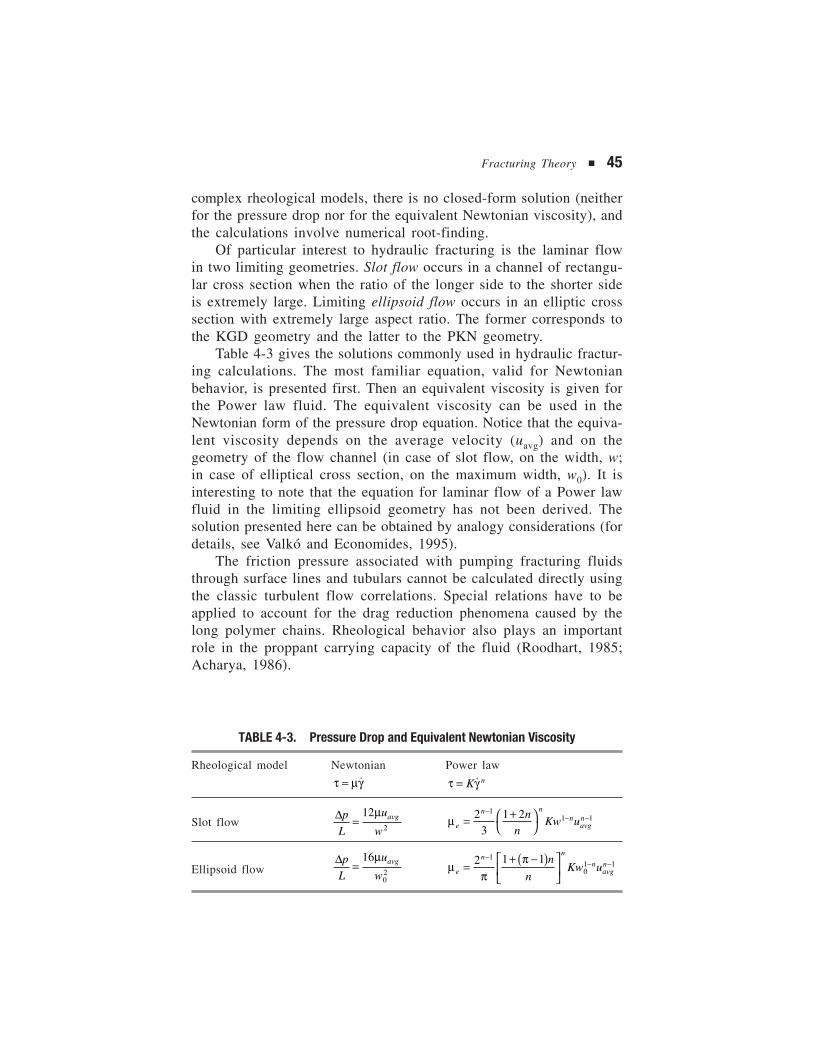
Fracturing Theory ■ 45
complex rheological models, there is no closed-form solution (neitherfor the pressure drop nor for the equivalent Newtonian viscosity), andthe calculations involve numerical root-finding.
Of particular interest to hydraulic fracturing is the laminar flowin two limiting geometries. Slot flow occurs in a channel of rectangu-lar cross section when the ratio of the longer side to the shorter sideis extremely large. Limiting ellipsoid flow occurs in an elliptic crosssection with extremely large aspect ratio. The former corresponds tothe KGD geometry and the latter to the PKN geometry.
Table 4-3 gives the solutions commonly used in hydraulic fractur-ing calculations. The most familiar equation, valid for Newtonianbehavior, is presented first. Then an equivalent viscosity is given forthe Power law fluid. The equivalent viscosity can be used in theNewtonian form of the pressure drop equation. Notice that the equiva-lent viscosity depends on the average velocity (uavg) and on thegeometry of the flow channel (in case of slot flow, on the width, w;in case of elliptical cross section, on the maximum width, w0). It isinteresting to note that the equation for laminar flow of a Power lawfluid in the limiting ellipsoid geometry has not been derived. Thesolution presented here can be obtained by analogy considerations (fordetails, see Valkó and Economides, 1995).
The friction pressure associated with pumping fracturing fluidsthrough surface lines and tubulars cannot be calculated directly usingthe classic turbulent flow correlations. Special relations have to beapplied to account for the drag reduction phenomena caused by thelong polymer chains. Rheological behavior also plays an importantrole in the proppant carrying capacity of the fluid (Roodhart, 1985;Acharya, 1986).
TABLE 4-3. Pressure Drop and Equivalent Newtonian Viscosity
Rheological model Newtonian Power law
τ µγ= ˙ τ γ= K n˙
Slot flow∆pL
u
wavg=
122
µµe
n nn
avgnn
nKw u= +
−− −2
31 21
1 1
Ellipsoid flow∆pL
u
wavg=
16
02
µµ
ππ
e
n n
navgnn
nKw u=
+ −( )
−− −2 1 11
01 1
46 ■ Unified Fracture Design
LEAKOFF AND VOLUME BALANCE IN THE FRACTURE
The polymer content of the fracturing fluid is partly intended to im-pede the loss of fluid into the reservoir. This phenomenon is envis-aged as a continuous build-up of a thin layer of polymer (the filtercake), which manifests an ever-increasing resistance to flow throughthe fracture face. The actual leakoff is determined by a coupled sys-tem that includes not only the filter cake, which is one element, butalso flow conditions in the reservoir.
A fruitful approximation dating back to Carter, 1957 (cf. appen-dix to Howard and Fast, 1957), is to consider the combined effect ofthe different phenomena as a material property. According to thisconcept, the leakoff velocity, vL , is given by the Carter I equation:
vC
tLL= (4-4)
where CL is the leakoff coefficient (length/time1/2 ) and t is the timeelapsed since the start of the leakoff process. The integrated form ofthe Carter equation is
V
A= 2C t + SLost
LL p (4-5)
where VLost is the fluid volume that passes through the surface AL
during the time period from time zero to time t. The integration con-stant, SP, is called the spurt loss coefficient. It can be considered asthe width of the fluid body passing through the surface instan-taneously at the very beginning of the leakoff process. Correspond-ingly, the term 2C tL can be considered as the leakoff width. (Notethat the factor 2 is an artifact of the integration. It has nothing to dowith the “two wings” and/or “two faces” introduced later.) The twocoefficients, CL and SP , can be determined from laboratory tests or,preferably, from evaluation of a fracture calibration test.
Formal Material Balance: The Opening-TimeDistribution Factor
Consider the fracturing treatment shown schematically in Figure 4-3.The volume Vi injected into one wing during the injection time te
consists of two parts: the volume of one fracture wing at the end of
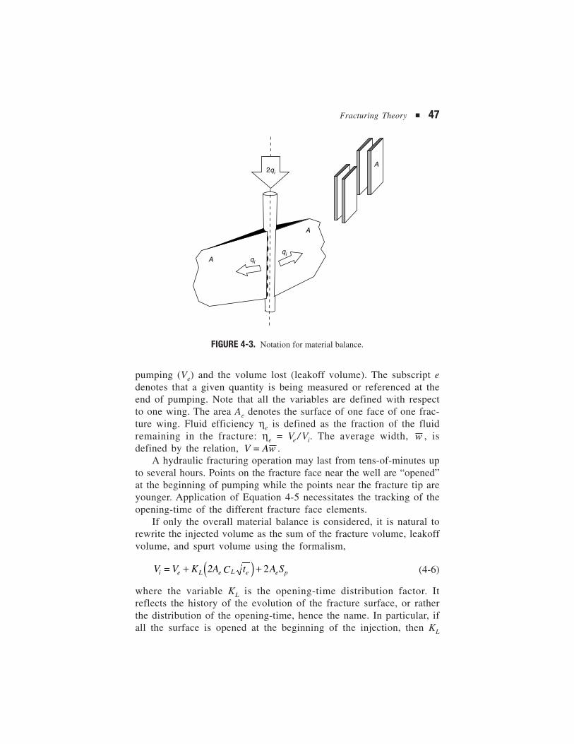
Fracturing Theory ■ 47
pumping (Ve) and the volume lost (leakoff volume). The subscript edenotes that a given quantity is being measured or referenced at theend of pumping. Note that all the variables are defined with respectto one wing. The area Ae denotes the surface of one face of one frac-ture wing. Fluid efficiency ηe is defined as the fraction of the fluidremaining in the fracture: ηe = Ve / Vi. The average width, w , isdefined by the relation, V Aw= .
A hydraulic fracturing operation may last from tens-of-minutes upto several hours. Points on the fracture face near the well are “opened”at the beginning of pumping while the points near the fracture tip areyounger. Application of Equation 4-5 necessitates the tracking of theopening-time of the different fracture face elements.
If only the overall material balance is considered, it is natural torewrite the injected volume as the sum of the fracture volume, leakoffvolume, and spurt volume using the formalism,
V = V K 2A C t A Si e L e L e e p+ ( ) + 2 (4-6)
where the variable KL is the opening-time distribution factor. Itreflects the history of the evolution of the fracture surface, or ratherthe distribution of the opening-time, hence the name. In particular, ifall the surface is opened at the beginning of the injection, then KL
FIGURE 4-3. Notation for material balance.
A
A
qi
2qi
A qi
48 ■ Unified Fracture Design
reaches its absolute maximum, KL = 2. The fluid efficiency is the ratioof the created volume to the injected volume. Dividing both volumesby the final fracture area, we can consider fracture efficiency as theratio of the created width to the would-be width, where the would-bewidth is defined as the sum of the created and lost widths.
Therefore, another form of Equation 4-6 is
ηee
e L L e p
w
w 2K C t S=
+ + 2 (4-7)
showing that the term 2K C tL L e can be considered as the “leakoffwidth,” and the term 2Sp as the “spurt width.” Equation 4-7 can berearranged to obtain the opening-time distribution factor in terms offluid efficiency and average width at the end of pumping:
KS
C t
w
2C t
w
2 C tLp
L e
e
L e
e
e L e
= − − +η (4-8)
Note that these relations are independent of the actual shape of thefracture face or the history of its evolution.
Constant Width Approximation (Carter Equation II)
In order to obtain an analytical solution for constant injection rate,Carter considered a hypothetical case in which the fracture widthremains constant during the fracture propagation (the width “jumps”to its final value in the first instant of pumping). Then a closed formexpression can be given for the fluid efficiency in terms of the twoleakoff parameters and the width:
ηπ
β β βπe
e e p
L e
w w S
C t=
+( ) ( ) ( ) + −
2
42
12
2exp erfc (4-9)
where βπ
=+
2
2
C t
w SL e
e p
.
Power Law Approximation to Surface Growth
A basic assumption postulated by Nolte (1979, 1986) leads to aremarkably simple form of the material balance. He assumed that thefracture surface evolves according to a power law,
Fracturing Theory ■ 49
A tD D= α (4-10)
where AD = A/Ae and tD = t/te , and the exponent α remains constantduring the entire injection period. Nolte realized that, in this case, theopening-time distribution factor is a function of α only. He representedthe opening-time distribution factor and its dependence on the exponentof fracture surface growth using the notation g0(α) and presented g0
for selected values of α. A simple expression first obtained by Hageland Meyer (1989) can be used to obtain the value of the opening-timedistribution factor for any α:
g0 2 3α πα α
α( ) = ( )
+( )Γ
Γ / (4-11)
where Γ(α) is the Euler gamma function.In calculations, the following approximation to the g0 function
might be easier to use:
g0
2 3
2 3 4α α α α
α α α α( ) = 2 + 2.06798 + 0.541262 + 0.0301598
1+1.6477 + 0.738452 + 0.0919097 + 0.00149497 (4-12)
Nolte assumed that the exponent remains between 0.5 and 1. Withthis assumption, the factor KL lies between 4/3 (1.33) and π/2 (1.57),indicating that for two extremely different surface growth histories,the opening-time distribution factor varies less than 20 percent. Gen-erally, the simple approximation KL = 1.5 should provide enoughaccuracy for design purposes.
Various practitioners have related the exponent α to fracturegeometry, fluid efficiency at the end of pumping, and fluid rheologi-cal behavior. None of these relations can be considered as proventheoretically, but they are reasonable engineering approximations,especially because the effect of the exponent on the final results islimited. Our recommendation is to use α = 4/5 for the PKN, α = 2/3for the KGD, and α = 8/9 for the radial model. These exponents canbe derived from the no-leakoff equations shown later in Table 4-4.
Numerically, the original constant-width approximation of Carterand the power law surface growth assumption of Nolte give very simi-lar results when used for design purposes. The g0-function approach does,however, have technical advantages when applied to the analysis ofcalibration treatments.
50 ■ Unified Fracture Design
Detailed Leakoff Models
The bulk leakoff model is not the only possible interpretation of theleakoff process. Several mechanistic models have been suggested inthe past (Williams, 1970 and Settari, 1985; Ehlig-Economides, et al.,1994; Yi and Peden, 1994; Mayerhofer, et al., 1995). The total pres-sure difference between the inside of a created fracture and a far pointin the reservoir is written as the sum,
∆ ∆ ∆ ∆p t p t p t p tface piz res( ) ( ) ( ) ( )= + + (4-13)
where ∆pface is the pressure drop across the fracture face dominatedby the filter cake, ∆ppiz is the pressure drop across a polymer-invadedzone and ∆pres is the pressure drop in the reservoir. Depending on theirsignificance under the given conditions, one or two terms may beneglected. While the first two terms are connected to the leakoff rateat a given time instant, the reservoir pressure drop is transient. Itdepends on the entire history of the leakoff process, not only on itsinstant intensity.
The detailed leakoff models hold an advantage in that they arebased on physically meaningful parameters, such as permeability andfilter cake resistance, and they allow for explicit pressure-dependentsimulation of the leakoff process. However, the application of thesemodels is limited by the complexity of the mathematics involved andby the extra input they require.
BASIC FRACTURE GEOMETRIES
Engineering models for the propagation of a hydraulically inducedfracture combine elasticity, fluid flow, material balance, and (in somecases) an additional propagation criterion. Given the fluid injectionhistory, a model should predict the evolution with time of the frac-ture dimensions and the wellbore pressure.
For design purposes, an approximate description of the geometrymight be sufficient, so simple models that predict fracture length andaverage width at the end of pumping are very useful. Models that pre-dict these two dimensions—while the third one, fracture height, is fixed—are referred to as 2D models. If the fracture surface is postulated topropagate in a radial fashion, that is, the height is not fixed, the modelis still considered to be 2D (the two dimensions being fracture radiusand width).
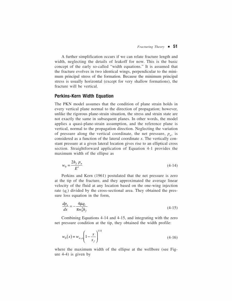
Fracturing Theory ■ 51
A further simplification occurs if we can relate fracture length andwidth, neglecting the details of leakoff for now. This is the basicconcept of the early so-called “width equations.” It is assumed thatthe fracture evolves in two identical wings, perpendicular to the mini-mum principal stress of the formation. Because the minimum principalstress is usually horizontal (except for very shallow formations), thefracture will be vertical.
Perkins-Kern Width Equation
The PKN model assumes that the condition of plane strain holds inevery vertical plane normal to the direction of propagation; however,unlike the rigorous plane-strain situation, the stress and strain state arenot exactly the same in subsequent planes. In other words, the modelapplies a quasi-plane-strain assumption, and the reference plane isvertical, normal to the propagation direction. Neglecting the variationof pressure along the vertical coordinate, the net pressure, pn , isconsidered as a function of the lateral coordinate x. The vertically con-stant pressure at a given lateral location gives rise to an elliptical crosssection. Straightforward application of Equation 4-1 provides themaximum width of the ellipse as
w =h p
Ef n
0
2
′(4-14)
Perkins and Kern (1961) postulated that the net pressure is zeroat the tip of the fracture, and they approximated the average linearvelocity of the fluid at any location based on the one-wing injectionrate (qi) divided by the cross-sectional area. They obtained the pres-sure loss equation in the form,
dp
dx
q
w hn i
f
= − 4
03
µπ (4-15)
Combining Equations 4-14 and 4-15, and integrating with the zeronet pressure condition at the tip, they obtained the width profile:
w x = wxxw o
f0
1 4
1( ) −
,
/
(4-16)
where the maximum width of the ellipse at the wellbore (see Fig-ure 4-4) is given by
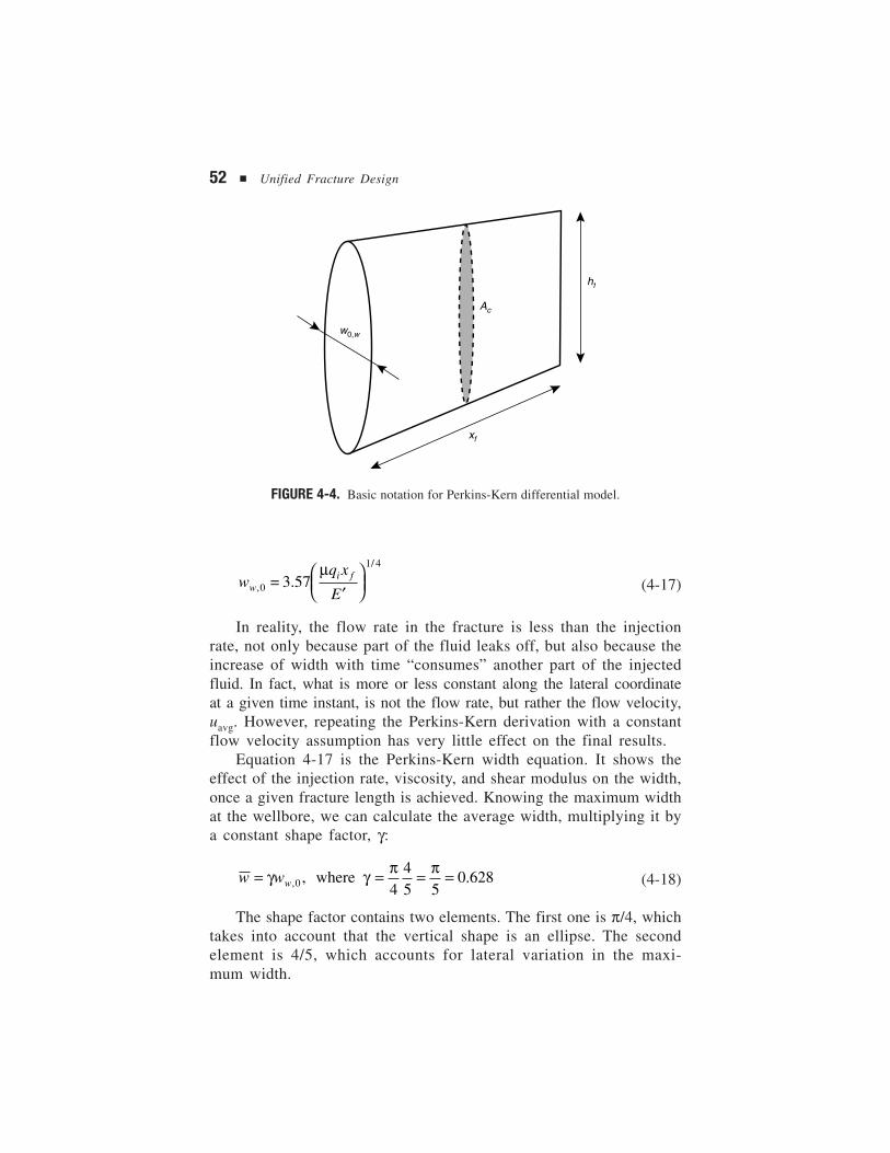
52 ■ Unified Fracture Design
FIGURE 4-4. Basic notation for Perkins-Kern differential model.
w =q x
Ewi f
,
/
.0
1 4
3 57µ
′
(4-17)
In reality, the flow rate in the fracture is less than the injectionrate, not only because part of the fluid leaks off, but also because theincrease of width with time “consumes” another part of the injectedfluid. In fact, what is more or less constant along the lateral coordinateat a given time instant, is not the flow rate, but rather the flow velocity,uavg. However, repeating the Perkins-Kern derivation with a constantflow velocity assumption has very little effect on the final results.
Equation 4-17 is the Perkins-Kern width equation. It shows theeffect of the injection rate, viscosity, and shear modulus on the width,once a given fracture length is achieved. Knowing the maximum widthat the wellbore, we can calculate the average width, multiplying it bya constant shape factor, γ:
w ww= = = =γ γ π π, ,0 4
45 5
where 0.628 (4-18)
The shape factor contains two elements. The first one is π/4, whichtakes into account that the vertical shape is an ellipse. The secondelement is 4/5, which accounts for lateral variation in the maxi-mum width.
Ac
hf
xf
w0,w
Fracturing Theory ■ 53
In the petroleum industry, a version of Equation 4-17 with aslightly different constant is used more often, and is referred to as thePerkins-Kern-Nordgren (PKN) width equation (Nordgren, 1972):
w =q x
Ewi f
,
/
.0
1 4
3 27µ
′
(4-19)
Khristianovich-Zheltov-Geertsma-deKlerk Width Equation
The first model of hydraulic fracturing, elaborated by Khristianovichand Zheltov (1955), envisioned a fracture with the same width at anyvertical coordinate within the fixed height, hf . The underlying physi-cal hypothesis is that the fracture faces slide freely at the top andbottom of the layer. The resulting fracture cross section is a rectangle.The width is considered as a function of the coordinate x. It is deter-mined from the plane-strain assumption, now applied in the (every)horizontal plane. The Khristianovich and Zheltov model containedanother interesting assumption: the existence of a non-wetted zone nearthe fracture tip. Geertsma and deKlerk (1969) accepted the mainassumptions of Khristianovich and Zheltov and reduced the model intoan explicit width formula. The KGD width equation is
w =q x
E h
q x
E hwi f
f
i f
f
3363 22
1 4 2 1 4 2 1 4
πµ µ
′
=
′
/
/ /
. (4-20)
In this case, the shape factor, relating the average width tothe wellbore width, has no vertical component. Then, because of theelliptical horizontal shape, we obtain
w ww= = =γ γ π, where 0.785
4(4-21)
Daneshy’s (1978) extension of the KGD model considers a non-constant pressure distribution along the fracture length, and a non-Newtonian fracturing fluid whose properties can change with time andtemperature. Numerical computations yield the specific leakoff, increasein width, and flow rate at points along the fracture length during frac-ture extension.
For short fractures, where 2xf < hf , the horizontal plane-strainassumption (KGD geometry) is more appropriate, and for 2xf > hf ,
54 ■ Unified Fracture Design
the vertical plane-strain assumption (PKN geometry) is physicallymore sound. Interestingly, for the special case when the total fracturelength and height are equivalent, the two equations give basically thesame average width and, hence, fracture volume.
Radial (Penny-shaped) Width Equation
This situation corresponds to horizontal fractures from vertical wells,vertical fractures extending from horizontal wells, or when fracturingrelatively thick homogeneous formations—from a limited perforationinterval in all cases. While the computations of fracture width aresensitive to how the fluid enters the fracture (a true point source wouldgive rise to infinite pressure), a reasonable model can be postulatedby analogy, which results in the same average width as the Perkins-Kern equation when Rf = xf = hf /2.
The result is
wq R
Ei f=′
2 241 4
./µ
(4-22)
The real significance of the simple models presented in this sec-tion is the insight they provide—helping us to consider the effect ofinput data on the evolving fracture. Additional insight can be gainedby comparing the fracture geometry and net pressure behavior ofthe models. Table 4-4 provides a direct side-by-side comparison of thebasic fracture models (no-leakoff case).
The last row in Table 4-4 deserves particular attention. For theno-leakoff case, net pressure increases with time for the Perkins-Kernmodel, but decreases with time for the other two models. This is awell-known result that raises some questions. For example, in mas-sive hydraulic fracturing, the net treating pressure most often increaseswith time, so net pressures derived from the Geertsma-deKlerk andradial models are of limited practical value. A more startling (and lesswell-known) observation is that the net pressures provided by theGeertsma-deKlerk and radial models are independent of injection rate.The KGD (and radial) view implies that when the fracture extentbecomes large, very low net pressures are required to maintain a cer-tain width. While this is a consequence of linear elasticity theory andthe way that the plane-strain assumption is applied, it leads to absurd
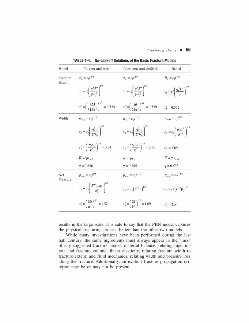
Fracturing Theory ■ 55
results in the large scale. It is safe to say that the PKN model capturesthe physical fracturing process better than the other two models.
While many investigations have been performed during the lasthalf century, the same ingredients must always appear in the “mix”of any suggested fracture model: material balance, relating injectionrate and fracture volume; linear elasticity, relating fracture width tofracture extent; and fluid mechanics, relating width and pressure lossalong the fracture. Additionally, an explicit fracture propagation cri-terion may be or may not be present.
TABLE 4-4. No-Leakoff Solutions of the Basic Fracture Models
Model Perkins and Kern Geertsma and deKlerk Radial
x c tf = 14 5/ x c tf = 1
2 3/ R c tf = 14 9/
c cq E
hi
f1 1
3
4
1 5
= ′ ′
µ
/
c cq E
hi
f1 1
3
3
1 6
= ′ ′
µ
/
c cq Ei
1 1
3 1 9
= ′ ′
µ
/
′ =
=c1 3
1 5625512
0 524π
/
. ′ =
=c1 3
1 61621
0 539π
/
. ′ =c1 0 572.
Width w = c tw,/
0 21 5 w = c tw 2
1 3/ w = c tw,/
0 21 9
c = cq
E hi
f2 2
21 5
′′
µ/
c = cq
E hi
f2 2
3
3
1 6
′′
µ/
c = cq
Ei
2 2
3 2
2
1 9
′′
µ/
′ =
=c2 2
1 525603 04
π
/
. ′
=c =2 3
1 653762 36
π
/
. ′c =2 3 65.
w = wwγ ,0 w = wwγ w = wwγ ,0
γ = 0.628 γ = 0.785 γ = 0.533
p c tn w,/= 3
1 5 p c tn w,/= −
31 3 p c tn w,
/= −3
1 3
c cE q
hi
f3 3
4 2
6
1 5
= ′ ′
µ/
c c E3 32 1 3
= ′ ′( )µ/
c c E3 32 1 3
= ′ ′( )µ/
′ =
=c3 2
1 4801 52
π
/
. ′ =
=c3
1 32116
1 09/
. ′ =c3 2 51.
FractureExtent
NetPressure

Fracturing of HighPermeability Formations5
57
THE EVOLUTION OF THE TECHNIQUE
As recently as the early 1990s, hydraulic fracturing was used almostexclusively for low permeability reservoirs. The large fluid leakoff andunconsolidated sands associated with high permeability formationswould ostensibly prevent the initiation and extension of a single, planarfracture with sufficient width to accept a meaningful proppant volume.Moreover, such fracture morphology, even if successfully created andpropped, would be incompatible with the defined needs of moderateto high permeability reservoirs, that is, large conductivity (width).
A key breakthrough tied to the advance of high permeabilityfracturing (HPF) is the tip screenout (TSO), which arrests lateralfracture growth and allows for subsequent fracture inflation andpacking. The result is short but wide to exceptionally wide fractures.While in traditional, unrestricted fracture growth an average fracturewidth of 0.25 in. would be considered normal, in TSO treatments,widths of one inch or even larger are commonly expected.
The role of hydraulic fracturing has expanded to encompass oilwells with permeabilities greater than 50 md and gas wells with over5 md of permeability (Table 5-1). These wells clearly require a TSOdesign. Because of these developments, hydraulic fracturing has
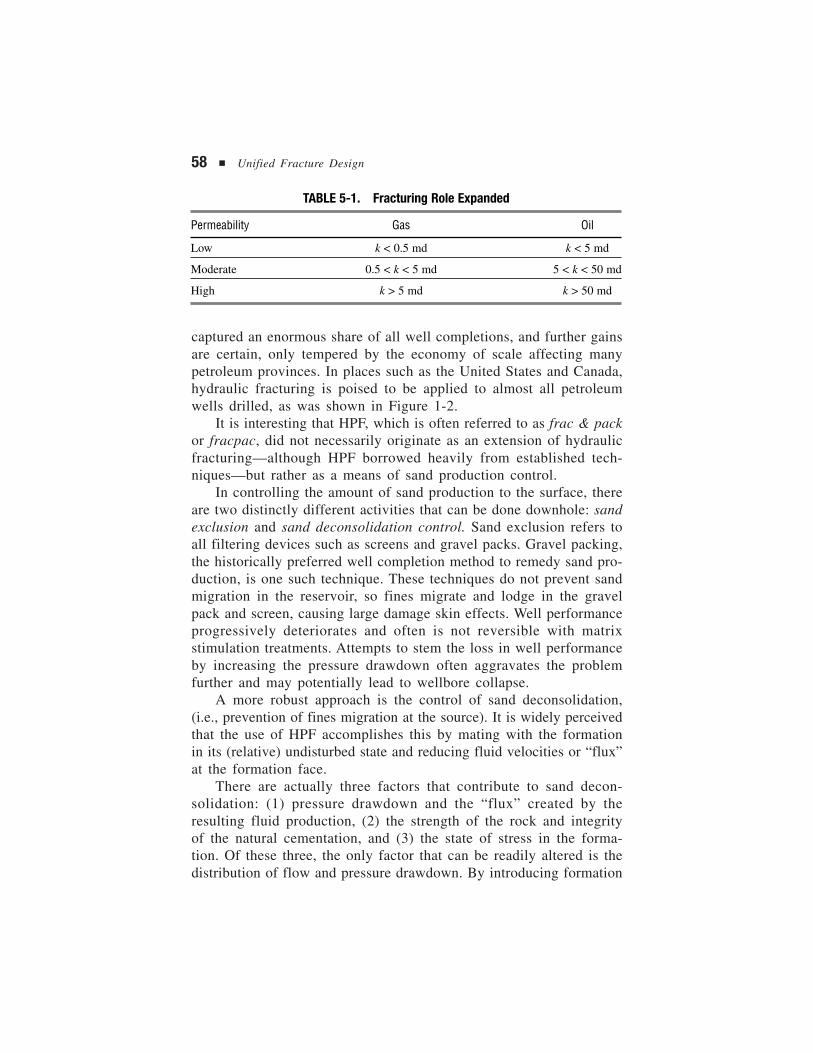
58 ■ Unified Fracture Design
captured an enormous share of all well completions, and further gainsare certain, only tempered by the economy of scale affecting manypetroleum provinces. In places such as the United States and Canada,hydraulic fracturing is poised to be applied to almost all petroleumwells drilled, as was shown in Figure 1-2.
It is interesting that HPF, which is often referred to as frac & packor fracpac, did not necessarily originate as an extension of hydraulicfracturing—although HPF borrowed heavily from established tech-niques—but rather as a means of sand production control.
In controlling the amount of sand production to the surface, thereare two distinctly different activities that can be done downhole: sandexclusion and sand deconsolidation control. Sand exclusion refers toall filtering devices such as screens and gravel packs. Gravel packing,the historically preferred well completion method to remedy sand pro-duction, is one such technique. These techniques do not prevent sandmigration in the reservoir, so fines migrate and lodge in the gravelpack and screen, causing large damage skin effects. Well performanceprogressively deteriorates and often is not reversible with matrixstimulation treatments. Attempts to stem the loss in well performanceby increasing the pressure drawdown often aggravates the problemfurther and may potentially lead to wellbore collapse.
A more robust approach is the control of sand deconsolidation,(i.e., prevention of fines migration at the source). It is widely perceivedthat the use of HPF accomplishes this by mating with the formationin its (relative) undisturbed state and reducing fluid velocities or “flux”at the formation face.
There are actually three factors that contribute to sand decon-solidation: (1) pressure drawdown and the “flux” created by theresulting fluid production, (2) the strength of the rock and integrityof the natural cementation, and (3) the state of stress in the forma-tion. Of these three, the only factor that can be readily altered is thedistribution of flow and pressure drawdown. By introducing formation
TABLE 5-1. Fracturing Role Expanded
Permeability Gas Oil
Low k < 0.5 md k < 5 md
Moderate 0.5 < k < 5 md 5 < k < 50 md
High k > 5 md k > 50 md
Fracturing of High Permeability Formations ■ 59
fluids to the well along a more elongated path (e.g., a hydraulicfracture or horizontal well), it is entirely possible to reduce the fluidflux and, in turn, control sand production.
Consider a simple example by assuming a well that penetrates a100 ft thick reservoir. If the well has a diameter equal to 1 ft, thenthe area for incoming radial flow in an open hole completion wouldbe about 300 ft2. However, for a fracture half-length of 100 ft, thearea of flow would be (2 × 100 × 100 × 2) 40,000 ft2. (Note: thesecond 2 accounts for the two walls of the fracture.) Remember thatin a fractured well almost all fluid flow would be from the reservoirinto the fracture, and then along the fracture into the well. For thesame production rate, this calculation suggests the fluid flux ina fractured well would be less than 1/100th the fluid flux in anunfractured well.
Of course, not a great deal can be done to affect the state of stressor formation competence. The magnitude of earth stresses dependsprimarily on reservoir depth and to some extent pressure, with thesituation becoming more complicated at depths of 3,000 ft or less.Pressure maintenance with gas or water flooding may be counter-productive unless maintenance of reservoir pressure allows economicproduction at a smaller drawdown. Various innovations have beensuggested to remedy incompetent formations or improve on naturalcementation—for example, by introducing complex well configurationsor various exotic chemical treatments—but there is little that can bedone to control this factor either.
In light of the discussion above, it should not be surprising thatHPF has replaced gravel packs in many petroleum provinces sus-ceptible to sand production, especially in operations where moresophisticated engineering is done. As with any stimulation techniquethat results in a productivity index improvement (defined as theproduction rate divided by the pressure drawdown), it is up to theoperator to allocate this new productivity index either to a larger rateor a lower drawdown, or any combination of the two.
HPF indicates a marked departure from the heritage of gravelpacking, incorporating more and more from hydraulic fracture tech-nology. This trend can be seen, for instance, in the fluids and proppantsapplied. While the original fracpack treatments involved sand sizes and“clean” fluids common to gravel packing, the typical proppant sizesfor hydraulic fracturing (20/40 mesh) now dominate. The increasedapplication of crosslinked fracturing fluids also illustrates the trend.
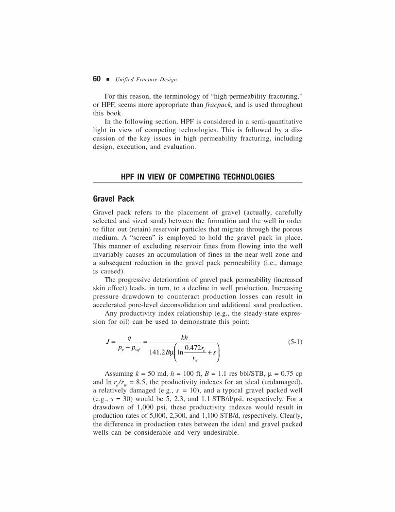
60 ■ Unified Fracture Design
For this reason, the terminology of “high permeability fracturing,”or HPF, seems more appropriate than fracpack, and is used throughoutthis book.
In the following section, HPF is considered in a semi-quantitativelight in view of competing technologies. This is followed by a dis-cussion of the key issues in high permeability fracturing, includingdesign, execution, and evaluation.
HPF IN VIEW OF COMPETING TECHNOLOGIES
Gravel Pack
Gravel pack refers to the placement of gravel (actually, carefullyselected and sized sand) between the formation and the well in orderto filter out (retain) reservoir particles that migrate through the porousmedium. A “screen” is employed to hold the gravel pack in place.This manner of excluding reservoir fines from flowing into the wellinvariably causes an accumulation of fines in the near-well zone anda subsequent reduction in the gravel pack permeability (i.e., damageis caused).
The progressive deterioration of gravel pack permeability (increasedskin effect) leads, in turn, to a decline in well production. Increasingpressure drawdown to counteract production losses can result inaccelerated pore-level deconsolidation and additional sand production.
Any productivity index relationship (e.g., the steady-state expres-sion for oil) can be used to demonstrate this point:
Jq
p pkh
Br
rse wf e
w
=−
=+
141 20 472
. ln.µ
(5-1)
Assuming k = 50 md, h = 100 ft, B = 1.1 res bbl/STB, µ = 0.75 cpand ln re/rw = 8.5, the productivity indexes for an ideal (undamaged),a relatively damaged (e.g., s = 10), and a typical gravel packed well(e.g., s = 30) would be 5, 2.3, and 1.1 STB/d/psi, respectively. For adrawdown of 1,000 psi, these productivity indexes would result inproduction rates of 5,000, 2,300, and 1,100 STB/d, respectively. Clearly,the difference in production rates between the ideal and gravel packedwells can be considerable and very undesirable.
Fracturing of High Permeability Formations ■ 61
Consider for a moment the use of high permeability fracturingunder the same scenario. This technology combines the advantages ofpropped fracturing to bypass the near-wellbore damage and gravelpacking to provide effective sand control. Figure 5-1 is the classicpresentation (compare Figure 3-6) of the equivalent skin effect (Cincoand Samaniego, 1978) in terms of dimensionless fracture conductivity,CfD (= kf w/kxf ), and fracture half-length, xf .
It can be seen from Figure 5-1 that even with a hydraulic fractureof less than optimum conductivity (e.g., CfD = 0.5) and short fracturelength (e.g., xf = 50 ft), the skin effect, sf (again using rw = 0.328 ft),would be equal to –3.
A negative skin effect equal to –3 applied to Equation 5-1 yieldsa productivity index of 7.7 STB/d/psi, more than a 50 percent increaseover the ideal PI and seven times the magnitude of a damaged gravel-packed well. Even with a damaged fracture (e.g., leakoff-induceddamage as described by Mathur et al., 1995) and a skin equal to –1,the productivity index would be 5.6 STB/d/psi, a five-fold increaseover a damaged gravel-packed well.
This calculation brings forward a simple, yet frequently over-looked, issue. Small negative skin values have a much greater impacton well performance than comparable magnitudes (absolute value) of
FIGURE 5-1. Pseudoskin factor for a vertical well intersected by a finite conductivity fracture.
4
3
2
1
00.1 1 10 100 1,000
CfD,opt
s f +
ln(x
f/r w
), y
sf + ln(xf /rw)
CfD,opt
y
62 ■ Unified Fracture Design
positive skin. Furthermore, in the example calculation here, a five-foldincrease in the productivity index suggests that the production ratewould increase by the same amount if the drawdown is held constant.Under an equally possible scenario, the production rate could be heldconstant and the drawdown reduced to one-fifth its original value. Anyother combination between these two limits can be envisioned.
The utility of high permeability fracturing is, thus, compelling—not just for production rate improvement, but also for the remedy ofundesirable drawdown-dependent phenomena.
High-Rate Water Packs
Empirical data reported by Tiner et al. (1996), as distilled and pre-sented in Table 5-2, support the frequent notion that high-rate waterpacks have an advantage over gravel packs, but do not afford theproductivity improvement of HPF. This improvement over gravel packsis reasonable by virtue of the additional proppant placed in the perfora-tion tunnels.
While not shown in the table, the performance of these com-pletions over time is also of interest. It is commonly reported thatproduction from high-rate water packs (as in the case of gravel packs)deteriorates with time. By contrast, Stewart et al. (1995), Mathur et al.(1995), and Ning et al. (1995) all report that production may pro-gressively improve (skin values decrease) during the first severalmonths following a HPF treatment.
PERFORMANCE OF FRACTURED HORIZONTAL WELLSIN HIGH PERMEABILITY FORMATIONS
Two of the most important developments in petroleum production inthe last 15 years are horizontal wells and high permeability fractur-ing. Considerable potential is possible by combining the two.
TABLE 5-2. Skin Values Reported by Tiner et al. (1996)
Gravel Pack High-Rate Water Pack HPF
+5 to +10 excellent +2 to +5 reported 0 to +2 normally
+40 and higher are reported 0 to –3 in some reports
Fracturing of High Permeability Formations ■ 63
Horizontal wells can be drilled either transverse or longitudinal tothe fracture azimuth. The transverse configuration is appropriate forlow permeability formations and has been widely used and documentedin the literature. The longitudinally fractured horizontal well warrantsfurther attention, specifically in the case of high permeability forma-tions. HPF often results in hydraulic fractures with low dimensionlessconductivities. Yet, such fractures installed longitudinally in horizontalwells in high permeability formations can have the net effect ofinstalling a (relative) high conductivity streak in an otherwise limitedconductivity flow conduit. Using a generic set of input data, Valkóand Economides (1996) showed discounted revenues for 15 cases thatdemonstrate this point.
Table 5-3 shows that for a given permeability, the potential forthe longitudinally fractured horizontal well is always higher than thatof a fractured vertical well and, with realistic fracture widths, mayapproach the theoretical potential of an infinite conductivity fracture.
Furthermore, the horizontal well fractured with 10-fold less proppant(CfD = 0.12) still outperforms the fractured vertical well for k = 1 and10 md, and is competitive at 100 md. The longitudinal configurationmay provide the additional benefit of avoiding excess breakdownpressures and tortuosity problems during execution.
DISTINGUISHING FEATURES OF HPF
The Tip Screenout Concept
The critical elements of HPF treatment design, execution, and inter-pretation are substantially different than for conventional fracture
TABLE 5-3. Discounted Revenue in US$ (1996) Millions
Configuration k = 1 md k = 10 md k = 100 md
Vertical well 0.73 6.4 57.7
Horizontal well 3.48 14.2 78.8
Fractured vertical well, CfD = 1.2 2.59 13.4 89.6
Fractured horizontal well, CfD = 1.2 3.88 16.3 95.8
Infinite-conductivity fracture (upper boundfor both horizontal and vertical well cases) 3.91 16.3 103.3
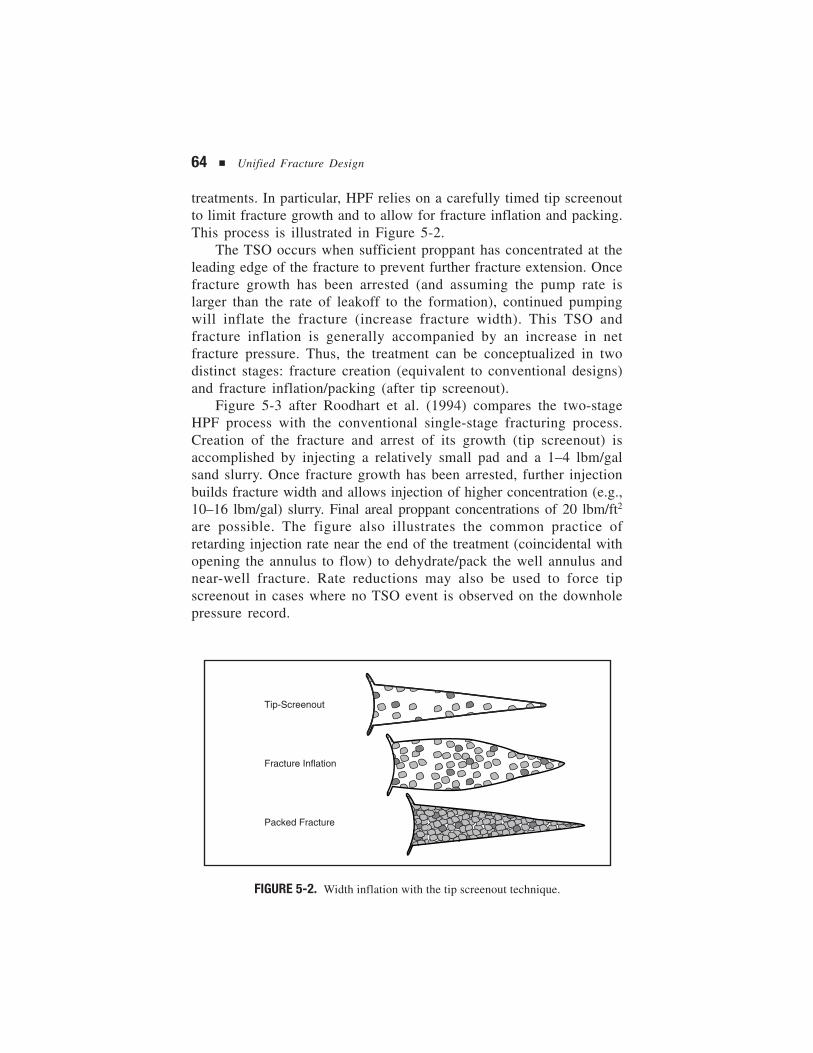
64 ■ Unified Fracture Design
treatments. In particular, HPF relies on a carefully timed tip screenoutto limit fracture growth and to allow for fracture inflation and packing.This process is illustrated in Figure 5-2.
The TSO occurs when sufficient proppant has concentrated at theleading edge of the fracture to prevent further fracture extension. Oncefracture growth has been arrested (and assuming the pump rate islarger than the rate of leakoff to the formation), continued pumpingwill inflate the fracture (increase fracture width). This TSO andfracture inflation is generally accompanied by an increase in netfracture pressure. Thus, the treatment can be conceptualized in twodistinct stages: fracture creation (equivalent to conventional designs)and fracture inflation/packing (after tip screenout).
Figure 5-3 after Roodhart et al. (1994) compares the two-stageHPF process with the conventional single-stage fracturing process.Creation of the fracture and arrest of its growth (tip screenout) isaccomplished by injecting a relatively small pad and a 1–4 lbm/galsand slurry. Once fracture growth has been arrested, further injectionbuilds fracture width and allows injection of higher concentration (e.g.,10–16 lbm/gal) slurry. Final areal proppant concentrations of 20 lbm/ft2
are possible. The figure also illustrates the common practice ofretarding injection rate near the end of the treatment (coincidental withopening the annulus to flow) to dehydrate/pack the well annulus andnear-well fracture. Rate reductions may also be used to force tipscreenout in cases where no TSO event is observed on the downholepressure record.
FIGURE 5-2. Width inflation with the tip screenout technique.
Tip-Screenout
Fracture Inflation
Packed Fracture

Fracturing of High Permeability Formations ■ 65
The tip screenout can be difficult to model, affect, or even detect.There are many reasons for this, including a tendency toward overlyconservative design models (resulting in no TSO), partial or multipletip screenout events, and inadequate pressure monitoring practices.
It is well accepted that accurate bottomhole measurements areimperative for meaningful treatment evaluation. Calculated bottomholepressures are unreliable because of the dramatic friction pressureeffects associated with pumping high sand concentrations throughsmall diameter tubulars and service tool crossovers. Surface data mayindicate that a TSO event has occurred when the bottomhole datashows no evidence, and vice versa. Even in the case of downholepressure data, there has been some discussion of where measurementsshould be taken. Friction and turbulence concerns have caused at leastone operator to conclude that bottomhole pressure data should becollected from below the crossover tool (washpipe gauges) in additionto data collected from the service tool bundle (Mullen et al., 1994).
The detection of tip screenout is discussed further in Chapter 10along with the introduction of a simple screening tool to evaluatebottomhole data.
FIGURE 5-3. Comparison of conventional and HPF design concepts.
- End of Job for Conventional Design -
BHP
Tip-Screenout
Injection Rate
Time
Injected SlurryConcentration
Fracture Creation
(Conventional)TSO
Fracture Inflation
and Packing
Fracturing Fluid and Proppant Concentrations in Fracture:
Pad Injection
Slurry Injection
At TSO
After FIP
66 ■ Unified Fracture Design
Net Pressure and Fluid Leakoff
The entire HPF process is dominated by net pressure and fluid leakoffconsiderations, first because high permeability formations are typicallysoft and exhibit low elastic modulus values, and second, because thefluid volumes are relatively small and leakoff rates high (high per-meability, compressible reservoir fluids, and non-wall-building fractur-ing fluids). Also, as described previously, the tip screenout design itselfaffects the net pressure. While traditional practices applicable todesign, execution, and evaluation in MHF continue to be used in HPF,these are frequently not sufficient.
Net Pressure, Closure Pressure,and Width in Soft Formations
Net pressure is the difference between the pressure at any point in thefracture and that of the fracture closure pressure. This definitioninvolves the existence of a unique closure pressure. Whether theclosure pressure is a constant property of the formation or dependsheavily on the pore pressure (or rather on the disturbance of the porepressure relative to the long term steady value) is an open question.
In high permeability, soft formations it is difficult (if not impossible)to suggest a simple recipe to determine the closure pressure as clas-sically derived from shut-in pressure decline curves (see Chapter 10).Furthermore, because of the low elastic modulus values, even small,induced uncertainties in the net pressure are amplified into largeuncertainties in the calculated fracture width.
Fracture Propagation
Fracture propagation, the availability of sophisticated 3D modelsnotwithstanding, presents complications in high permeability forma-tions, which are generally soft and have low elastic modulus values.For example, Chudnovsky (1996) emphasized the stochastic characterof this propagation. Also, because of the low modulus values, aninability to predict net pressure behavior may lead to a significantdeparture between predicted and actual treatment performance.
It is now a common practice to “predict” fracture propagation andnet pressure features using a computer fracture simulator. This trendof substituting clear models and physical assumptions with “knobs”—such as arbitrary stress barriers, friction changes (attributed to erosion,
Fracturing of High Permeability Formations ■ 67
if decreasing, and sand resistance, if increasing) and less-than-wellunderstood properties of the formation expressed as dimensionless“factors”—does not help to clarify the issue.
LEAKOFF MODELS FOR HPF
Considerable effort has been expended on laboratory investigation ofthe fluid leakoff process for high permeability cores. A comprehensivereport can be found in Vitthal and McGowen (1996) and McGowenand Vitthal (1996). The results raise some questions about how effectivelyfluid leakoff can be limited by filter cake formation.
In all cases, but especially in high permeability formations, thequality of the fracturing fluid is only one of the factors that influenceleakoff, and often not the determining one. Transient fluid flow in theformation might have an equal or even larger impact. Transient flowcannot be understood by simply fitting an empirical equation tolaboratory data. The use of models based on solutions to the fluid flowequation in porous media is an unavoidable step.
In the following, three models are considered that describe fluidleakoff in the high permeability environment. The traditional Carterleakoff model requires some modification for use in HPF as shown.(Note: While this model continues to be used across the industry,it is not entirely sufficient for the HPF application.) An alternate,filter cake leakoff model has been developed based on the work byMayerhofer, et al. (1993). The most appropriate leakoff model for highpermeability formations may be that of Fan and Economides (1995),which considers the series resistance caused by the filter cake, thepolymer-invaded zone, and the reservoir. While the Carter model is incommon use, the models of Mayerhofer, et al. and Fan and Economidesrepresent important building blocks and provide a conceptual frameworkfor understanding the key issue of leakoff in high permeability fracturing.
Fluid Leakoff and Spurt Loss as Material Properties: TheCarter Leakoff Model with Nolte’s Power Law Assumption
There are two main schools of thought concerning leakoff. The firstconsiders the phenomenon as a material property of the fluid/rocksystem. The basic relation (called the integrated Carter equation, givenalso in Chapter 4) is given in consistent units as
68 ■ Unified Fracture Design
V
A= 2C t + SL
LL p (5-2)
where AL is the area and VL is the total volume lost during the timeperiod from time zero to time t. To make use of material balance, theterm VL must be described. For rigorous theoretical development, VLis the volume of liquid entering the formation through the two createdfracture surfaces of one wing. The integration constant, Sp , is calledthe spurt loss coefficient and is measured in units of length. It can beconsidered as the width of the fluid body passing through the surfaceinstantaneously at the very beginning of the leakoff process, while2C tL is the width of the fluid body following the first slug. Thetwo coefficients, CL and Sp , can be determined from laboratory orfield tests.
As discussed in more detail in Chapter 4, Equation 5-2 can bevisualized assuming that the given surface element “remembers” whenit has been opened to fluid loss and has its own “zero” time that islikely different from that of other elements along the fracture surface.Points on the fracture face near the well are opened at the beginningof pumping while the points at the fracture tip are younger. Applicationof Equation 5-2 or its differential form necessitates tracking theopening time for different fracture-face elements, as discussed inChapter 4.
The second school of thought considers leakoff as a consequenceof flow mechanisms in the porous medium, and employs a cor-responding mathematical description.
Filter Cake Leakoff Model According to Mayerhofer, et al.
The method of Mayerhofer, et al. (1993) describes the leakoff rateusing two parameters that are physically more realistic than the leak-off coefficient: (1) filter cake resistance at a reference time and(2) reservoir permeability. It is assumed that these parameters (R0, thereference resistance at a reference time t0, and kr , the reservoir per-meability) have been identified from a minifrac diagnostic test. Inaddition, reservoir pressure, reservoir fluid viscosity, porosity, and totalcompressibility are assumed to be known.
Total pressure gradient from inside a created fracture out into thereservoir, ∆p, at any time during the injection, can be written as
∆ ∆ ∆ ∆p t p t p t p tface piz res( ) ( ) ( ) ( )= + + (5-3)
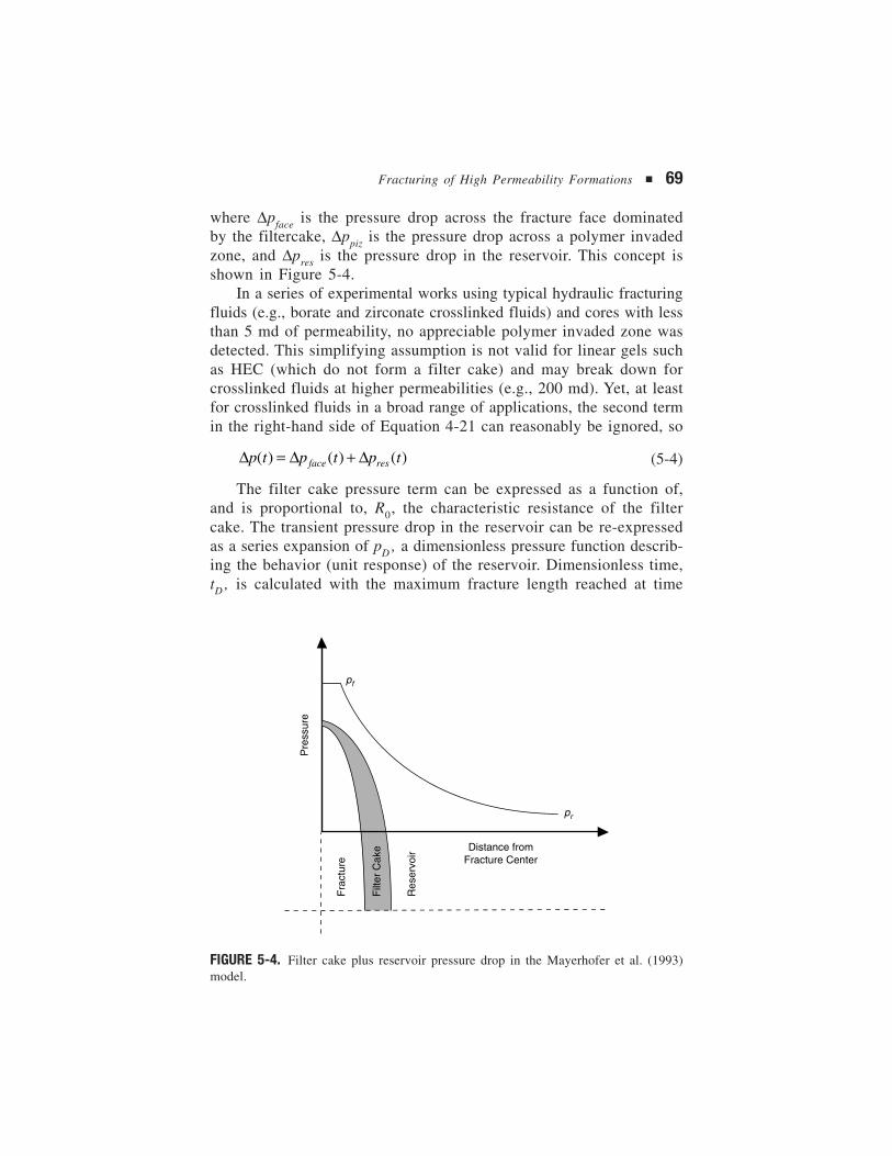
Fracturing of High Permeability Formations ■ 69
where ∆pface is the pressure drop across the fracture face dominatedby the filtercake, ∆ppiz is the pressure drop across a polymer invadedzone, and ∆pres is the pressure drop in the reservoir. This concept isshown in Figure 5-4.
In a series of experimental works using typical hydraulic fracturingfluids (e.g., borate and zirconate crosslinked fluids) and cores with lessthan 5 md of permeability, no appreciable polymer invaded zone wasdetected. This simplifying assumption is not valid for linear gels suchas HEC (which do not form a filter cake) and may break down forcrosslinked fluids at higher permeabilities (e.g., 200 md). Yet, at leastfor crosslinked fluids in a broad range of applications, the second termin the right-hand side of Equation 4-21 can reasonably be ignored, so
∆ ∆ ∆p t p t p tface res( ( () ) )= + (5-4)
The filter cake pressure term can be expressed as a function of,and is proportional to, R0, the characteristic resistance of the filtercake. The transient pressure drop in the reservoir can be re-expressedas a series expansion of pD , a dimensionless pressure function describ-ing the behavior (unit response) of the reservoir. Dimensionless time,tD , is calculated with the maximum fracture length reached at time
FIGURE 5-4. Filter cake plus reservoir pressure drop in the Mayerhofer et al. (1993)model.
Pre
ssur
e
pf
pr
Distance fromFracture Center
Res
ervo
ir
Fra
ctur
e
Filt
er C
ake
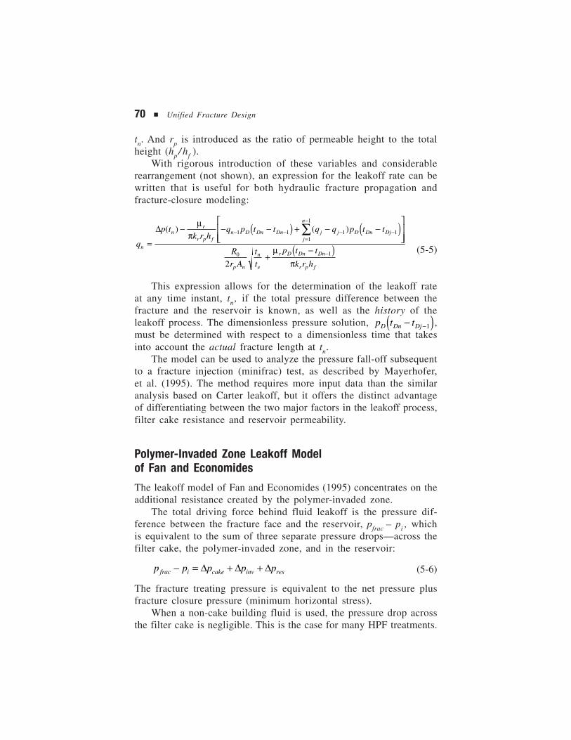
70 ■ Unified Fracture Design
tn. And rp is introduced as the ratio of permeable height to the totalheight (hp / hf ).
With rigorous introduction of these variables and considerablerearrangement (not shown), an expression for the leakoff rate can bewritten that is useful for both hydraulic fracture propagation andfracture-closure modeling:
q
p tk r h
q p t t q q p t t
R
r A
t
t
p t t
k r h
n
nr
r p fn D Dn Dn j
j
n
j D Dn Dj
p n
n
e
r D Dn Dn
r p f
=
− − −( ) + − −( )
+−( )
− −=
−
− −
−
∑∆ ( ) ( )µ
π
µπ
1 11
1
1 1
0 1
2
(5-5)
This expression allows for the determination of the leakoff rateat any time instant, tn , if the total pressure difference between thefracture and the reservoir is known, as well as the history of theleakoff process. The dimensionless pressure solution, p t tD Dn Dj−( )−1 ,must be determined with respect to a dimensionless time that takesinto account the actual fracture length at tn.
The model can be used to analyze the pressure fall-off subsequentto a fracture injection (minifrac) test, as described by Mayerhofer,et al. (1995). The method requires more input data than the similaranalysis based on Carter leakoff, but it offers the distinct advantageof differentiating between the two major factors in the leakoff process,filter cake resistance and reservoir permeability.
Polymer-Invaded Zone Leakoff Modelof Fan and Economides
The leakoff model of Fan and Economides (1995) concentrates on theadditional resistance created by the polymer-invaded zone.
The total driving force behind fluid leakoff is the pressure dif-ference between the fracture face and the reservoir, pfrac – pi , whichis equivalent to the sum of three separate pressure drops—across thefilter cake, the polymer-invaded zone, and in the reservoir:
p p p p pfrac i cake inv res− = + +∆ ∆ ∆ (5-6)
The fracture treating pressure is equivalent to the net pressure plusfracture closure pressure (minimum horizontal stress).
When a non-cake building fluid is used, the pressure drop acrossthe filter cake is negligible. This is the case for many HPF treatments.
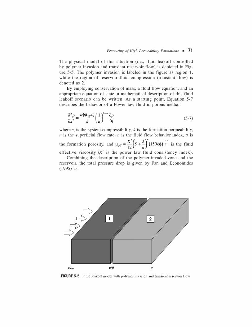
Fracturing of High Permeability Formations ■ 71
The physical model of this situation (i.e., fluid leakoff controlledby polymer invasion and transient reservoir flow) is depicted in Fig-ure 5-5. The polymer invasion is labeled in the figure as region 1,while the region of reservoir fluid compression (transient flow) isdenoted as 2.
By employing conservation of mass, a fluid flow equation, and anappropriate equation of state, a mathematical description of this fluidleakoff scenario can be written. As a starting point, Equation 5-7describes the behavior of a Power law fluid in porous media:
∂∂
φµ ∂∂
2
2
11px
n c
k upt
eff tn
=
−
(5-7)
where ct is the system compressibility, k is the formation permeability,u is the superficial flow rate, n is the fluid flow behavior index, φ is
the formation porosity, and µ φeff
n nKn
k= ′ +
( )
−
129
3150
12 is the fluid
effective viscosity (K� is the power law fluid consistency index).Combining the description of the polymer-invaded zone and the
reservoir, the total pressure drop is given by Fan and Economides(1995) as
FIGURE 5-5. Fluid leakoff model with polymer invasion and transient reservoir flow.
pfrac pis(t)
1 2
72 ■ Unified Fracture Design
p pk
e erf
e erfc
frac r
app
r
− =
+
π φηµ α η
α
µ α ηα
ηα
ηα
2
4
4
4
1
4
2
1
2
2
2
1
2
(5-8)
where ak
nu
ceff
n
t
1 11=
−
φµ and a
kct
2 =φµ
.
At given conditions, Equation 5-8 can be solved iteratively for theparameter η (not to be confused with fluid efficiency). Once the valueof η is found for a specified total pressure drop, the leakoff rate iscalculated from
q AtL =
ηφ2
1(5-9)
In other words, the factor η/(2φ) can be considered a pressure-dependent apparent leakoff coefficient.
FRACTURING HIGH PERMEABILITYGAS CONDENSATE RESERVOIRS
In gas condensate reservoirs, a situation emerges very frequently thatis tantamount to fracture face damage. Because of the pressure gradi-ent that is created normal to the fracture, liquid condensate is formed,which has a major impact on the reduction of the relative permeabil-ity to gas. Such a reduction depends on the phase behavior of the fluidand the penetration of liquid condensate, which in turn, depends onthe pressure drawdown imposed on the well. These phenomena causean apparent damage that affects the performance of all fractured wells,but especially those with high reservoir permeability.
Wang, et al. (2000) presented a model that predicts the fracturedwell performance in gas condensate reservoirs, quantifying the effectsof gas permeability reduction. Furthermore, they presented fracturetreatment design for condensate reservoirs. The distinguishing feature
Fracturing of High Permeability Formations ■ 73
primarily affects the required fracture length to offset the problemsassociated with the emergence of liquid condensate.
Gas relative permeability curves were derived using a pore-scalenetwork model and are represented by a weighted linear function ofimmiscible and miscible relative permeability curves:
k fk f krg rgI rgM= + −( )1 (5-10)
where krg is the gas relative permeability, and f is a weighing factorthat is a function of the capillary number,
fN
ac
b=+
1
11/
(5-11)
The numerical values for a and b are 1.6 × 10⁻³ and 0.324,respectively, and Nc is the capillary number, defined as
Nk p
c =∇σ (5-12)
In Equation 5-12, k is the permeability, ∇p is the pressure gradient,and σ is the interfacial tension. The conventional relative permeabilityfor capillary dominated (immiscible) flow in Equation 5-10, krgI , isdefined as
kS
SrgIg
wi
ng
=−
1 (5-13)
where Sg is the gas saturation, Swi is the connate water saturation, andng is a constant equal to 5.5. The relative permeability function in thelimit of viscous dominated (miscible) flow, krgM , is defined as
kS
SrgMg
wi
=−1 (5-14)
Recall that Cinco and Samaniego (1981) provided an expres-sion of the fracture face skin effect that is additive to the dimen-sionless pressure for the finite conductivity fracture performance:
sb
xkkfs
s
f s
= −
π2
1 (5-15)
where bs is the penetration of damage and ks is the damaged permeability.
74 ■ Unified Fracture Design
An analogy can readily be made for a hydraulically fractured gascondensate reservoir. Liquid condensate that drops out normal to thefracture face can also result in a skin effect, in this case reflecting areduction in the relative permeability to gas. The penetration ofdamage would be the zone inside which liquid condensate exists (i.e.,the dew point pressure establishes the boundary).
The permeability ratio reduces to the ratio of the relative per-meabilities, and because at the boundary kr g is equal to 1, Equa-tion 5-15 becomes simply,
sb
x kfss
f rg
= −
π2
11 (5-16)
Optimizing Fracture Geometryin Gas Condensate Reservoirs
In gas condensate reservoirs, the fracture performance is likely to beaffected greatly by the presence of liquid condensate, tantamount tofracture face damage. An assumption for the evaluation is that thereservoir pressure at the boundary of this “damaged” zone must beexactly equal to the dew point pressure.
For any fracture length and a given flowing bottomhole pressureinside the retrograde condensation zone of a two-phase envelope, thepressure profile normal to the fracture phase and into the reservoir willdelineate the points where the pressure is equal to the dew pointpressure. From this pressure profile, the distribution of fracture faceskin can be determined. The depth of the affected zone is determinedfrom Equation 5-16, the modified Cinco-Ley and Samaniego expres-sion. An additional necessary element is the relative permeabilityimpairment given by the correlation presented in Equations 5-10 to 5-14.
Two example case studies are presented below. The first representsa reservoir with 5 md permeability and a gas condensate with a dewpoint pressure of 2,545 psi. The flowing bottomhole pressure is 1,800psi. First, a standard hydraulic fracture optimization—ignoring theeffects of the fracture face skin—using a proppant number, Nprop, equalto 0.02, results in an expected dimensionless fracture conductivity of1.6 and a fracture half-length of 220 ft for a 4,000 ft square reservoir.(The value of the proppant number, assuming kf = 50,000 md, h = 50 ft,ρp = 165 lb/ft3 and φp = 0.4, implies a proppant mass approximatelyequal to 80,000 lbm.) The dimensionless productivity index would be 0.35.
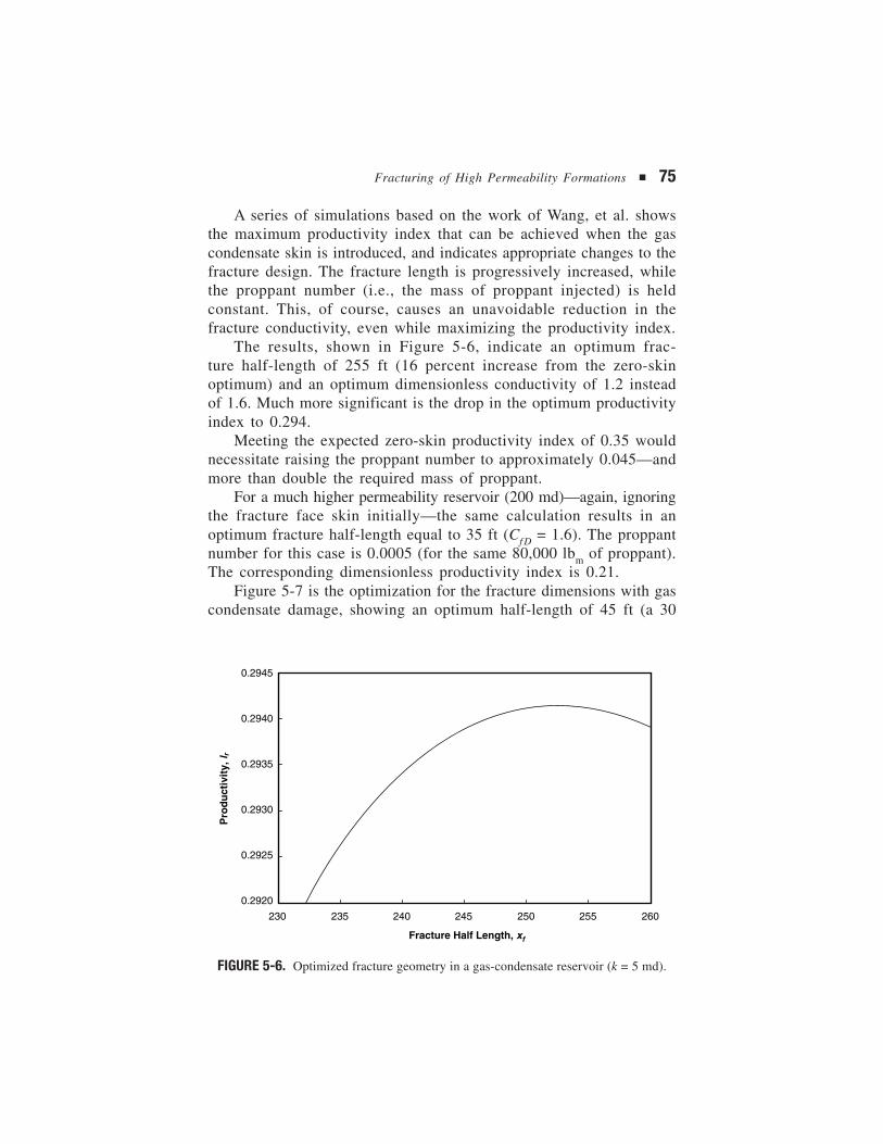
Fracturing of High Permeability Formations ■ 75
A series of simulations based on the work of Wang, et al. showsthe maximum productivity index that can be achieved when the gascondensate skin is introduced, and indicates appropriate changes to thefracture design. The fracture length is progressively increased, whilethe proppant number (i.e., the mass of proppant injected) is heldconstant. This, of course, causes an unavoidable reduction in thefracture conductivity, even while maximizing the productivity index.
The results, shown in Figure 5-6, indicate an optimum frac-ture half-length of 255 ft (16 percent increase from the zero-skinoptimum) and an optimum dimensionless conductivity of 1.2 insteadof 1.6. Much more significant is the drop in the optimum productivityindex to 0.294.
Meeting the expected zero-skin productivity index of 0.35 wouldnecessitate raising the proppant number to approximately 0.045—andmore than double the required mass of proppant.
For a much higher permeability reservoir (200 md)—again, ignoringthe fracture face skin initially—the same calculation results in anoptimum fracture half-length equal to 35 ft (Cf D = 1.6). The proppantnumber for this case is 0.0005 (for the same 80,000 lbm of proppant).The corresponding dimensionless productivity index is 0.21.
Figure 5-7 is the optimization for the fracture dimensions with gascondensate damage, showing an optimum half-length of 45 ft (a 30
FIGURE 5-6. Optimized fracture geometry in a gas-condensate reservoir (k = 5 md).
0.2945
0.2940
0.2935
0.2930
0.2925
0.2920
230 235 240 245 250 255 260
Fracture Half Length, xf
Pro
du
ctiv
ity,
l r
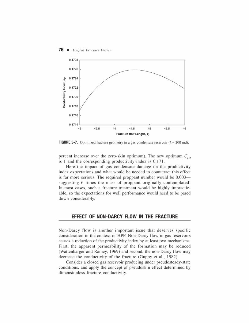
76 ■ Unified Fracture Design
percent increase over the zero-skin optimum). The new optimum Cf Dis 1 and the corresponding productivity index is 0.171.
Here the impact of gas condensate damage on the productivityindex expectations and what would be needed to counteract this effectis far more serious. The required proppant number would be 0.003—suggesting 6 times the mass of proppant originally contemplated!In most cases, such a fracture treatment would be highly impractic-able, so the expectations for well performance would need to be pareddown considerably.
EFFECT OF NON-DARCY FLOW IN THE FRACTURE
Non-Darcy flow is another important issue that deserves specificconsideration in the context of HPF. Non-Darcy flow in gas reservoirscauses a reduction of the productivity index by at least two mechanisms.First, the apparent permeability of the formation may be reduced(Wattenbarger and Ramey, 1969) and second, the non-Darcy flow maydecrease the conductivity of the fracture (Guppy et al., 1982).
Consider a closed gas reservoir producing under pseudosteady-stateconditions, and apply the concept of pseudoskin effect determined bydimensionless fracture conductivity.
FIGURE 5-7. Optimized fracture geometry in a gas-condensate reservoir (k = 200 md).
0.1728
0.1726
0.1724
0.1722
0.1720
0.1718
0.1716
0.171443 43.5 44 44.5 45 45.5 46
Fracture Half Length, xf
Pro
du
ctiv
ity
Ind
ex, J
D
Fracturing of High Permeability Formations ■ 77
Definitions and Assumptions
Gas production is calculated from the pseudosteady-state deliverabilityequation:
qkhT m p m p
p T
k
k f Cr
x
sc wf
sc
r app
r fD appe
f
=( ) − ( )[ ]
×
( ) +
π,
, ln.
10 472
(5-17)
where m(p) is the pseudopressure function, kf,app is the apparent per-meability of the proppant in the fracture, and kr,app is the apparentpermeability of the formation. (All equations in this subsection aregiven for a consistent system of units, such as SI.) The function f wasintroduced by Cinco-Ley and Samaniego (1981) and was presented inChapter 3 as
f C sx
r. . u . u
. u . u . ufD ff
w1
2
2 3
165 0 328 01161 018 0 064 0 005
( ) = + = − ++ + +
lnln (5-18)
where u = lnCfD.The apparent dimensionless fracture conductivity is defined by
Ck w
k xfD appf app
r app f,
,
,
= (5-19)
The apparent permeabilities are flow-rate dependent; therefore, thedeliverability equation becomes implicit in the production rate.
Proceeding further requires a model of non-Darcy flow. Almostexclusively, the Forcheimer equation is used:
− = +dpdx k
v v vµ βρ (5-20)
where ν = qa /A is the Darcy velocity and β is a property of the porousmedium.
A popular correlation was presented by Firoozabadi and Katz(1979) as
β = ck1 2. (5-21)
where c = 8.4 × 10⁻⁸ m1.4 (= 2.6 × 1010 ft–1 md1.2).

78 ■ Unified Fracture Design
To apply the Firoozabadi and Katz correlation, we write
− = +
= +
dpdx
vk
k vv
k
c v
kµ β ρ
µµ ρ
µ1
11
10 2. (5-22)
showing that
k
k c v
k
app =+
1
10 2
ρµ.
(5-23)
The equation above can be used both for the reservoir and for thefracture if correct representative linear velocity is substituted. In thefollowing, it is assumed that h = hf .
A representative linear velocity for the reservoir can be given interms of the gas production rate as
vq
hxa
f
=4 (5-24)
where qa is the in-situ (actual) volumetric flow rate; hence, for thereservoir non-Darcy effect,
c vk
c q
h x kr
a
f r
ρµ
ρµ0 2 0 22
12. .
=
(5-25)
A representative linear velocity in the fracture can be given interms of the gas production rate as
vq
hwa=
2(5-26)
Thus, for the non-Darcy effect in the fracture, one can use
c vk
c q
h wkf
a
f
ρµ
ρµ0 2 0 22
1. .
=
(5-27)
The term ρqa is the mass flow rate and is the same in the reservoirand in the fracture; cρqa is expressed in terms of the gas productionrate as
c q
h
c
hq c qa a gρ
µρ γµ2 2 0= = (5-28)
where q is the gas production rate in standard volume per time, γg isthe specific gravity of gas with respect to air, and ρa is the density of
Fracturing of High Permeability Formations ■ 79
air at standard conditions. The factor c0 is constant for a givenreservoir-fracture system.
The final form of the apparent permeability dependence on pro-duction rate is
k
k c q
x k
app
r
f r
=+
1
12
00 2.
(5-29)
for the reservoir and
k
k c q
wk
app
f
f
=+
1
1 00 2.
(5-30)
for the fracture. As a consequence, the deliverability equation becomes
qkhT m p m p
p T c q
x kf C
r
x
sc wf
sc
f rfD app
e
f
=( ) − ( )[ ]
×
+
( ) +
π 1
12
0 47200 2 1. , ln
. (5-31)
where
Ck w
k x
c
wkq
c
x kq
fD appf
r f
f
f r
,
.
.
=+
+
1
12
00 2
00 2
(5-32)
The additional skin effect, sND , appearing because of non-Darcyflow, can be expressed as
sc q
x kf C
r
xf C
r
xNDf r
fD appe
ffD
e
f
= +
( ) +
− ( ) +
12
0 472 0 47200 2 1 1. , ln
.ln
.(5-33)
The additional non-Darcy skin effect is always positive and depends onthe production rate in a nonlinear manner.
Equations 5-31 and 5-33 are of primary importance to interpretpost-fracture well testing data and to forecast production. If themechanism responsible for the post-treatment skin effect is not under-stood clearly, the evaluation of the treatment and the productionforecast might be severely erroneous.
80 ■ Unified Fracture Design
Case Study for the Effect of Non-Darcy Flow
As previously discussed, non-Darcy flow in a gas reservoir causes areduction of the productivity index by at least two mechanisms. First,the apparent permeability of the formation may be reduced, andsecond, the non-Darcy flow may decrease the fracture conductivity.In this case study, the effect of non-Darcy flow on production ratesand observed skin effects is investigated.
Reservoir and fracture properties are given in Table 5-4.A simplified form of Equation 5-30 in field units is
qp p
ZTk h
c q
x kf C
r
x
wf
rf r
fD appe
f
=−
×
+
( ) +
2 2
00 2 1
14241
12
0 472µ. , ln
. (5-34)
where cc
ha g
0 2=
ρ γµ
must be expressed in ft-md0.2/MMSCF/day. In the
given example, c0 = 73 ft-md0.2/MMSCF/day and
Ck w
k x
c
x kq
c
wkq
k w
k x
c q
c qfD appf
r f
f r
f
f
r f
r
f,
.
=
+
+=
++
12
1
11
00 2
00 2
0
0
.
(5-35)
where c0r = 2.34 × 10⁻³ m3/s = 7.67 × 10⁻² (MSCF/day)–1
c0f = 6.14 × 10 –1 m3/s = 2.78 × 10² (MSCF/day)–1
Therefore, in field units
CqqfD app, .
.= ++
1 391 0 761 280
and (5-36)
qp
q f C
wf
fD app
=−
×+( ) ( ) +[ ]
4000
21 6451
1 0 76 3 16
2 2
1. . .,
(5-37)
The non-Darcy component of the skin effect can be calculated as
s q f CND fD app= +( ) ( ) +[ ]−1 0 00076 3 16 4 6191. . ., (5-38)
The results are shown graphically in Figures 5-8 to 5-10.
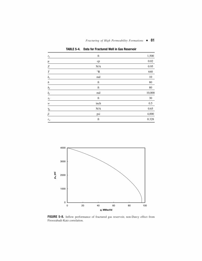
Fracturing of High Permeability Formations ■ 81
FIGURE 5-8. Inflow performance of fractured gas reservoir, non-Darcy effect fromFiroozabadi-Katz correlation.
TABLE 5-4. Data for Fractured Well in Gas Reservoir
re ft 1,500
µ cp 0.02
Z N/A 0.95
T °R 640
kr md 10
h ft 80
hf ft 80
kf md 10,000
xf ft 30
w inch 0.5
γg N/A 0.65
p– psi 4,000
rw ft 0.328
4000
3000
2000
1000
00 20 40 60 80 100
q, MMscf/d
pw
, psi
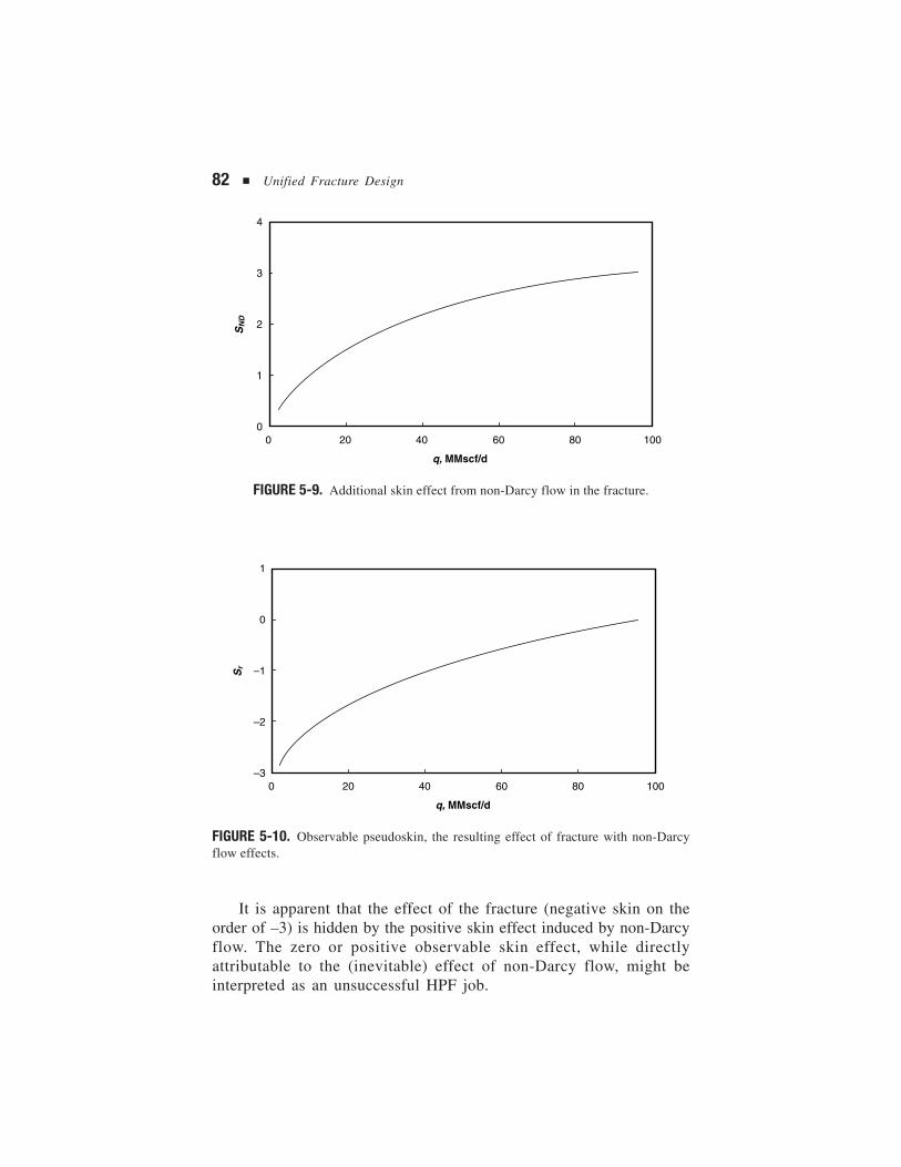
82 ■ Unified Fracture Design
FIGURE 5-10. Observable pseudoskin, the resulting effect of fracture with non-Darcyflow effects.
FIGURE 5-9. Additional skin effect from non-Darcy flow in the fracture.
It is apparent that the effect of the fracture (negative skin on theorder of –3) is hidden by the positive skin effect induced by non-Darcyflow. The zero or positive observable skin effect, while directlyattributable to the (inevitable) effect of non-Darcy flow, might beinterpreted as an unsuccessful HPF job.
4
3
2
1
00 20 40 60 80 100
q, MMscf/d
SN
D
1
0
–1
–2
–30 20 40 60 80 100
q, MMscf/d
Sr
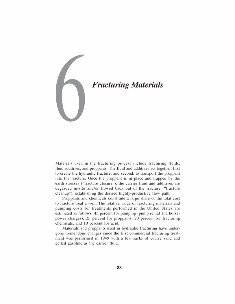
Fracturing Materials6
83
Materials used in the fracturing process include fracturing fluids,fluid additives, and proppants. The fluid and additives act together, firstto create the hydraulic fracture, and second, to transport the proppantinto the fracture. Once the proppant is in place and trapped by theearth stresses (“fracture closure”), the carrier fluid and additives aredegraded in-situ and/or flowed back out of the fracture (“fracturecleanup”), establishing the desired highly-productive flow path.
Proppants and chemicals constitute a large share of the total costto fracture treat a well. The relative value of fracturing materials andpumping costs for treatments performed in the United States areestimated as follows: 45 percent for pumping (pump rental and horse-power charges), 25 percent for proppants, 20 percent for fracturingchemicals, and 10 percent for acid.
Materials and proppants used in hydraulic fracturing have under-gone tremendous changes since the first commercial fracturing treat-ment was performed in 1949 with a few sacks of coarse sand andgelled gasoline as the carrier fluid.
84 ■ Unified Fracture Design
FRACTURING FLUIDS
The fracturing fluid transmits hydraulic pressure from the pumps tothe formation, which creates a fracture, and then transports proppant(hence the name carrier fluid) into the created fracture. The invasivefluids are then removed (or cleaned up) from the formation, allowingthe production of hydrocarbons. Factors to consider when selecting thefluid include availability, safety, ease of mixing and use, viscositycharacteristics, compatibility with the formation, ability to be cleanedup from the fracture, and cost.
Fracturing fluids can be categorized as (1) oil- or water-base,usually “crosslinked” to provide the necessary viscosity, (2) mixturesof oil and water, called emulsions, and (3) foamed oil- and water-basesystems that contain nitrogen or carbon dioxide gas. Oil-based fluidswere used almost exclusively in the 1950s. By the 1990s, more than90 percent of fracturing fluids were crosslinked water-based systems.Today, nitrogen and carbon dioxide systems in water-based fluids areused in about 25 percent of fracture stimulation jobs.
Table 6-1 lists the most common fracturing fluids in order ofcurrent usage. The choice of which crosslinking method to use is based
TABLE 6-1. Crosslinked Fluid Types
ApplicationCrosslinker Gelling Agent pH Range Temperature
B, non-delayed Guar, HPG 8–12 70–300 °F
B, delayed Guar, HPG 8–12 70–300 °F
Zr, delayed Guar 7–10 150–300 °F
Zr, delayed Guar 5–8 70–250 °F
Zr, delayed CMHPG, HPG 9–11 200–400 °F
Zr-a, delayed CMHPG 3–6 70–275 °F
Ti, non-delayed Guar, HPG, CMHPG 7–9 100–325 °F
Ti, delayed Guar, HPG, CMHPG 7–9 100–325 °F
Al, delayed CMHPG 4–6 70–175 °F
Sb, non-delayed Guar, HPG 3–6 60–120 °F
a—compatible with carbon dioxide
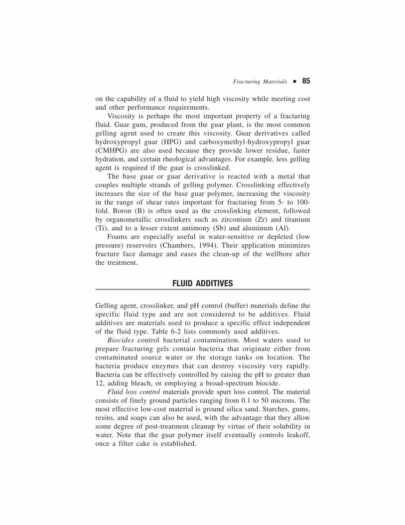
Fracturing Materials ■ 85
on the capability of a fluid to yield high viscosity while meeting costand other performance requirements.
Viscosity is perhaps the most important property of a fracturingfluid. Guar gum, produced from the guar plant, is the most commongelling agent used to create this viscosity. Guar derivatives calledhydroxypropyl guar (HPG) and carboxymethyl-hydroxypropyl guar(CMHPG) are also used because they provide lower residue, fasterhydration, and certain rheological advantages. For example, less gellingagent is required if the guar is crosslinked.
The base guar or guar derivative is reacted with a metal thatcouples multiple strands of gelling polymer. Crosslinking effectivelyincreases the size of the base guar polymer, increasing the viscosityin the range of shear rates important for fracturing from 5- to 100-fold. Boron (B) is often used as the crosslinking element, followedby organometallic crosslinkers such as zirconium (Zr) and titanium(Ti), and to a lesser extent antimony (Sb) and aluminum (Al).
Foams are especially useful in water-sensitive or depleted (lowpressure) reservoirs (Chambers, 1994). Their application minimizesfracture face damage and eases the clean-up of the wellbore afterthe treatment.
FLUID ADDITIVES
Gelling agent, crosslinker, and pH control (buffer) materials define thespecific fluid type and are not considered to be additives. Fluidadditives are materials used to produce a specific effect independentof the fluid type. Table 6-2 lists commonly used additives.
Biocides control bacterial contamination. Most waters used toprepare fracturing gels contain bacteria that originate either fromcontaminated source water or the storage tanks on location. Thebacteria produce enzymes that can destroy viscosity very rapidly.Bacteria can be effectively controlled by raising the pH to greater than12, adding bleach, or employing a broad-spectrum biocide.
Fluid loss control materials provide spurt loss control. The materialconsists of finely ground particles ranging from 0.1 to 50 microns. Themost effective low-cost material is ground silica sand. Starches, gums,resins, and soaps can also be used, with the advantage that they allowsome degree of post-treatment cleanup by virtue of their solubility inwater. Note that the guar polymer itself eventually controls leakoff,once a filter cake is established.
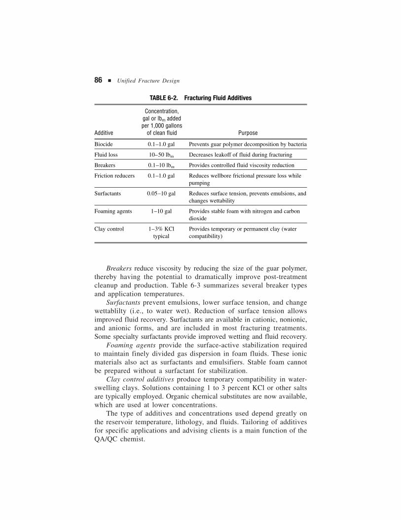
86 ■ Unified Fracture Design
Breakers reduce viscosity by reducing the size of the guar polymer,thereby having the potential to dramatically improve post-treatmentcleanup and production. Table 6-3 summarizes several breaker typesand application temperatures.
Surfactants prevent emulsions, lower surface tension, and changewettablilty (i.e., to water wet). Reduction of surface tension allowsimproved fluid recovery. Surfactants are available in cationic, nonionic,and anionic forms, and are included in most fracturing treatments.Some specialty surfactants provide improved wetting and fluid recovery.
Foaming agents provide the surface-active stabilization requiredto maintain finely divided gas dispersion in foam fluids. These ionicmaterials also act as surfactants and emulsifiers. Stable foam cannotbe prepared without a surfactant for stabilization.
Clay control additives produce temporary compatibility in water-swelling clays. Solutions containing 1 to 3 percent KCl or other saltsare typically employed. Organic chemical substitutes are now available,which are used at lower concentrations.
The type of additives and concentrations used depend greatly onthe reservoir temperature, lithology, and fluids. Tailoring of additivesfor specific applications and advising clients is a main function of theQA/QC chemist.
TABLE 6-2. Fracturing Fluid Additives
Concentration,gal or lbm addedper 1,000 gallons
Additive of clean fluid Purpose
Biocide 0.1–1.0 gal Prevents guar polymer decomposition by bacteria
Fluid loss 10–50 lbm Decreases leakoff of fluid during fracturing
Breakers 0.1–10 lbm Provides controlled fluid viscosity reduction
Friction reducers 0.1–1.0 gal Reduces wellbore frictional pressure loss whilepumping
Surfactants 0.05–10 gal Reduces surface tension, prevents emulsions, andchanges wettability
Foaming agents 1–10 gal Provides stable foam with nitrogen and carbondioxide
Clay control 1–3% KCl Provides temporary or permanent clay (water typical compatibility)
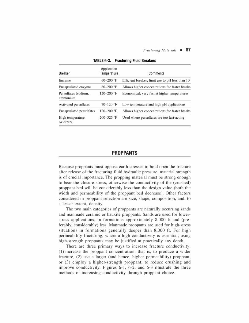
Fracturing Materials ■ 87
PROPPANTS
Because proppants must oppose earth stresses to hold open the fractureafter release of the fracturing fluid hydraulic pressure, material strengthis of crucial importance. The propping material must be strong enoughto bear the closure stress, otherwise the conductivity of the (crushed)proppant bed will be considerably less than the design value (both thewidth and permeability of the proppant bed decrease). Other factorsconsidered in proppant selection are size, shape, composition, and, toa lesser extent, density.
The two main categories of proppants are naturally occurring sandsand manmade ceramic or bauxite proppants. Sands are used for lower-stress applications, in formations approximately 8,000 ft and (pre-ferably, considerably) less. Manmade proppants are used for high-stresssituations in formations generally deeper than 8,000 ft. For highpermeability fracturing, where a high conductivity is essential, usinghigh-strength proppants may be justified at practically any depth.
There are three primary ways to increase fracture conductivity:(1) increase the proppant concentration, that is, to produce a widerfracture, (2) use a larger (and hence, higher permeability) proppant,or (3) employ a higher-strength proppant, to reduce crushing andimprove conductivity. Figures 6-1, 6-2, and 6-3 illustrate the threemethods of increasing conductivity through proppant choice.
TABLE 6-3. Fracturing Fluid Breakers
ApplicationBreaker Temperature Comments
Enzyme 60–200 °F Efficient breaker; limit use to pH less than 10
Encapsulated enzyme 60–200 °F Allows higher concentrations for faster breaks
Persulfates (sodium, 120–200 °F Economical; very fast at higher temperaturesammonium
Activated persulfates 70–120 °F Low temperature and high pH applications
Encapsulated persulfates 120–200 °F Allows higher concentrations for faster breaks
High temperature 200–325 °F Used where persulfates are too fast-actingoxidizers
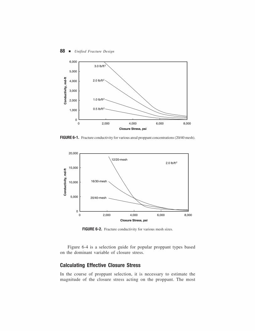
88 ■ Unified Fracture Design
FIGURE 6-1. Fracture conductivity for various areal proppant concentrations (20/40 mesh).
FIGURE 6-2. Fracture conductivity for various mesh sizes.
Figure 6-4 is a selection guide for popular proppant types basedon the dominant variable of closure stress.
Calculating Effective Closure Stress
In the course of proppant selection, it is necessary to estimate themagnitude of the closure stress acting on the proppant. The most
6,000
5,000
4,000
3,000
2,000
1,000
00 2,000 4,000 6,000 8,000
Closure Stress, psi
Co
nd
uct
ivit
y, m
d-f
t3.0 lb/ft2
2.0 lb/ft2
1.0 lb/ft2
0.5 lb/ft2
20,000
15,000
10,000
5,000
00 2,000 4,000 6,000 8,000
Closure Stress, psi
Co
nd
uct
ivit
y, m
d-f
t
2.0 lb/ft212/20-mesh
16/30-mesh
20/40-mesh
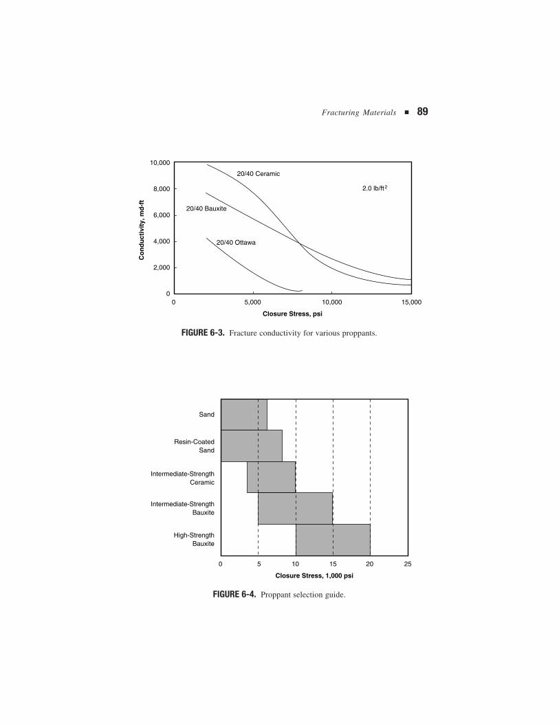
Fracturing Materials ■ 89
FIGURE 6-3. Fracture conductivity for various proppants.
FIGURE 6-4. Proppant selection guide.
10,000
8,000
6,000
4,000
2,000
00 5,000 10,000 15,000
Closure Stress, psi
Co
nd
uct
ivit
y, m
d-f
t
2.0 lb/ft2
20/40 Ceramic
20/40 Bauxite
20/40 Ottawa
Sand
Resin-CoatedSand
Intermediate-StrengthCeramic
Intermediate-StrengthBauxite
High-StrengthBauxite
0 5 10 15 20 25
Closure Stress, 1,000 psi
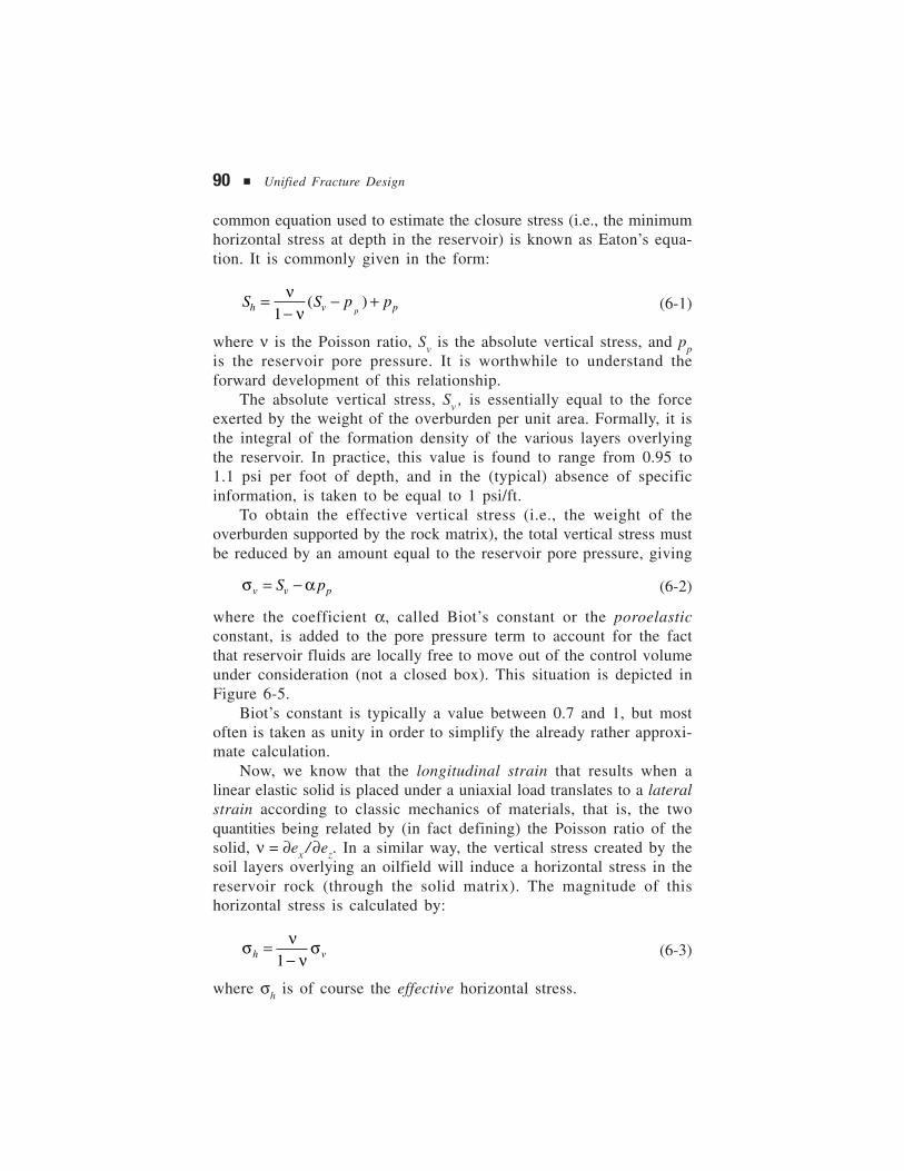
90 ■ Unified Fracture Design
common equation used to estimate the closure stress (i.e., the minimumhorizontal stress at depth in the reservoir) is known as Eaton’s equa-tion. It is commonly given in the form:
S S p ph v pp=
−− +ν
ν1( ) (6-1)
where ν is the Poisson ratio, Sv is the absolute vertical stress, and ppis the reservoir pore pressure. It is worthwhile to understand theforward development of this relationship.
The absolute vertical stress, Sv , is essentially equal to the forceexerted by the weight of the overburden per unit area. Formally, it isthe integral of the formation density of the various layers overlyingthe reservoir. In practice, this value is found to range from 0.95 to1.1 psi per foot of depth, and in the (typical) absence of specificinformation, is taken to be equal to 1 psi/ft.
To obtain the effective vertical stress (i.e., the weight of theoverburden supported by the rock matrix), the total vertical stress mustbe reduced by an amount equal to the reservoir pore pressure, giving
σ αv v pS p= − (6-2)
where the coefficient α, called Biot’s constant or the poroelasticconstant, is added to the pore pressure term to account for the factthat reservoir fluids are locally free to move out of the control volumeunder consideration (not a closed box). This situation is depicted inFigure 6-5.
Biot’s constant is typically a value between 0.7 and 1, but mostoften is taken as unity in order to simplify the already rather approxi-mate calculation.
Now, we know that the longitudinal strain that results when alinear elastic solid is placed under a uniaxial load translates to a lateralstrain according to classic mechanics of materials, that is, the twoquantities being related by (in fact defining) the Poisson ratio of thesolid, ν = ∂ex / ∂ez. In a similar way, the vertical stress created by thesoil layers overlying an oilfield will induce a horizontal stress in thereservoir rock (through the solid matrix). The magnitude of thishorizontal stress is calculated by:
σ νν
σh v=−1
(6-3)
where σh is of course the effective horizontal stress.
Fracturing Materials ■ 91
Combining Equations 6-2 and 6-3 and rearranging slightly,
S S p ph v pp=
−− +ν
να α
1( ) (6-4)
which, taking Biot’s constant to be equal to 1, yields the common formof Eaton’s equation.
Now, it is important to recognize that, unless the producing bottom-hole pressure in the fracture treated well is drawn down to somewherenear zero, the entire burden of this horizontal stress will not be borneby the proppant. Another important observation is that the horizontalstress in the reservoir is itself a function of reservoir pore pressure,so the closure stress on the proppant is nominally reduced withreservoir depletion.
FRACTURE CONDUCTIVITY ANDMATERIALS SELECTION IN HPF
Fracture Width as a Design Variable
A great deal has been published concerning optimum fracture dimen-sions in HPF. While there are debates regarding the optimum, fracture
FIGURE 6-5. Poroelasticity.
Force
GrainsPore Fluid
α ~ 0.7 to 1.0
Effective Stress = Total Stress – α (Pore Pressure)
92 ■ Unified Fracture Design
width is largely regarded as more important than fracture length. Ofcourse, this is an intuitive statement and only recognizes the firstprinciple of fracture optimization: higher permeability formationsrequire higher fracture conductivity to maintain an acceptable valueof the dimensionless fracture conductivity, CfD.
A “rule of thumb” is that fracture length should be equal to 1/2of the perforation height (thickness of producing interval). Hunt et al.(1994) showed that cumulative recovery from a well in a 100 mdreservoir with a 10 ft damage radius is optimized by extending a fixed8,000 md-ft conductivity fracture to any appreciable distance beyondthe damaged zone. This result implies that there is little benefit to a50 ft fracture length compared to a 10 ft fracture length. Two observa-tions may be in order. First, the Hunt et al. evaluation is based oncumulative recovery. Second, their assumption of a fixed fractureconductivity implies a decreasing dimensionless fracture conductivitywith increasing fracture length (i.e., less than optimal placement ofthe proppant).
It is generally true that if an acceptable CfD is maintained—this mayrequire an increase in areal proppant concentration from 1.5 lbm/ft2,which is common in hard-rock fracturing, to 20 lbm/ft2 or more—additional length will provide additional production. As explained inChapter 3, the optimum fracture conductivity of 1.6 corresponds tothe best compromise between the capacity of the fracture to conductand the capacity of the reservoir to deliver fluids. This applies to highpermeability and low permeability formations alike.
The problem, in practice, has been that fracture extent and widthare difficult to influence separately. Historically, once a fracturing fluidand injection rate are selected, the fracture width evolves with increas-ing length according to strict relations (at least in the well-known PKNand KGD design models). Therefore, the key decision variable hasbeen the fracture extent. After the fracture extent is determined, thewidth is calculated as a consequence of technical limitations (e.g.,maximum realizable proppant concentration). Knowledge of the leakoffprocess helps to determine the necessary pumping time and pad volume.
The tip screenout technique has brought a significant change tothis design philosophy. Through TSO, fracture width can be increasedwithout increasing the fracture extent. Now we have a very effectivemeans to design and execute fractures that satisfy the optimum condition.
The ultimate decision requires optimizing the mass of proppantbased on economics or, in cases where total fluid and proppant
Fracturing Materials ■ 93
volumes are physically limited (e.g., in offshore environments), opti-mizing placement of a finite proppant volume
Proppant Selection
The primary and unique issue relating to proppant selection for highpermeability fracturing, beyond maintaining a high permeability at anystress, is proppant sizing. While specialty proppants such as intermediatestrength and resin-coated proppants have certainly been employed in HPF,the majority of treatments are pumped with standard graded-mesh sand.
When selecting a proppant size for HPF, the engineer faces competingpriorities: size the proppant to address concerns with sand exclusion,or use maximum proppant size to ensure adequate fracture conductivity.
As with equipment choices and fluids selection, the gravel-packingroots of frac & pack are also evident when it comes to proppantselection. Engineers initially focused on sand exclusion and a gravelpack derived sizing criteria such as that proposed by Saucier (1974).Saucier recommends that the mean gravel size (Dg50 ) be five to sixtimes the mean formation grain size (Df 50). The so-called “4-by-8 rule”implies minimum and maximum grain-size diameters that are distri-buted around Saucier’s criteria (i.e., Dg,min = 4Dg 50 and Dg,max = 8Dg50 ,respectively). Thus, many early treatments were pumped with standard40/60 mesh or even 50/70 mesh sand. The somewhat limited con-ductivity of these gravel pack mesh sizes under in-situ formationstresses is not adequate in many cases. Irrespective of sand mesh size,frac & packs tend to reduce concerns with fines migration by virtueof reducing fluid flux at the formation face.
The current trend in proppant selection is to use fracturing-sizesand. A typical HPF treatment now employs 20/40 proppant (sand).Maximizing the fracture conductivity can itself help prevent sandproduction by virtue of reducing drawdown. Results with the largerproppant have been encouraging, both in terms of productivity andlimiting or eliminating sand production (Hannah et al., 1993).
It is interesting to note that the topics of formation competenceand sanding tendency, major issues in the realm of gravel pack tech-nology, have not been widely studied in the context of HPF. It seemsthat in many cases HPF is providing a viable solution to comple-tion failures in spite of the industry’s primitive understanding of (soft)rock mechanics.
94 ■ Unified Fracture Design
This move away from gravel pack practices toward fracturing-typepractices is common to many aspects of HPF with the exception (sofar) of downhole tools, and it seems to justify the migration in ourterminology from frac & pack to high permeability fracturing. Thefollowing discussion of fluid selection is consistent with this perspective.
Fluid Selection
Fluid selection for HPF has always been driven by concerns withdamaging the high permeability formation, either by filter cake buildupor (especially) polymer invasion. Most early treatments were carriedout using HEC, the classic gravel pack fluid, as it was perceived tobe less damaging than guar-based fracturing fluids. While the debatehas lingered on and while some operators continue to use HEC fluids,the fluid of choice is increasingly borate-crosslinked HPG.
Based on a synthesis of reported findings from several practi-tioners, Aggour and Economides (1996) provide a rationale to guidefluid selection in HPF. Their findings suggest that if the extent offracturing fluid invasion is minimized, the degree of damage (i.e.,permeability impairment caused by filter cake or polymer invasion)is of secondary importance. They employ the effective skin repre-sentation of Mathur et al. (1995) to show that if fluid leakoff penetra-tion is small, even severe permeability impairments can be toleratedwithout exhibiting positive skin effects. In this case, the obviousrecommendation in HPF is to use high polymer concentration, cross-linked fracturing fluids with fluid-loss additives, and an aggressivebreaker schedule. The polymer, crosslinker, and fluid-loss additiveslimit polymer invasion, and the breaker ensures maximum fractureconductivity, a critical factor which cannot be overlooked.
Experimental work corroborates these contentions. Linear gelshave been known to penetrate cores of very low permeability (1 mdor less) whereas crosslinked polymers are likely to build filter cakesat permeabilities two orders of magnitude higher (Roodhart, 1985;Mayerhofer et al., 1991). Filter cakes, while they may damage thefracture face, clearly reduce the extent of polymer penetration into thereservoir normal to the fracture face. At extremely high permeabilities,even crosslinked polymer solutions may invade the formation.
Cinco-Ley and Samaniego (1981) and Cinco-Ley et al. (1978)described the performance of finite-conductivity fractures and delineatedthree major types of damage affecting this performance.
Fracturing Materials ■ 95
■ Reduction of proppant pack permeability resulting from eitherproppant crushing or (especially) unbroken polymer chains leadsto fracture conductivity impairment. This can be particularlyproblematic in moderate to high permeability reservoirs. Exten-sive progress in breaker technology has dramatically reducedconcerns with this type of damage.
■ Choke damage refers to the near-well zone of the fracture, whichcan be accounted for by a skin effect. This damage can result fromeither over-displacement at the end of a treatment or by finesmigration during production. In the latter case, one can envisionfines from the formation or proppant accumulating near the wellbut within the fracture.
■ Fracture face damage implies permeability reduction normal tothe fracture face, including permeability impairments caused bythe filter cake, polymer-invaded, and filter cake-invaded zones.
Composite Skin Effect
Mathur et al. (1995) provide the following representation for effectiveskin resulting from radial wellbore damage and fracture face damage:
sb k
b k x b k
b b k
b k x b k
b
xdr
f
r
f r f
=+ −( ) +
−( )+ −( ) −
π2
2
1 3 1 2
1 2
1 1 1
1(6-5)
Figure 6-6 depicts the two types of damage accounted for in sd(i.e., fracture-face and radial wellbore damage).
The b- and k- terms are defined graphically in Figure 6-7 andrepresent the dimensions and permeabilities of various zones includedin the finite conductivity fracture model of Mathur et al.
The equivalent damage skin can be added directly to the undamagedCinco and Samaniego fracture skin effect to obtain the total skin,
s s st d f= + (6-6)
Parametric Studies
Aggour and Economides (1996) employed the Mathur et al. model(with no radial wellbore damage) to evaluate total skin and investigatethe relative effects of different variables. Their results related the totalskin in a number of discrete cases to (1) the depth of fluid invasionnormal to the fracture face and (2) the degree of permeability reduction
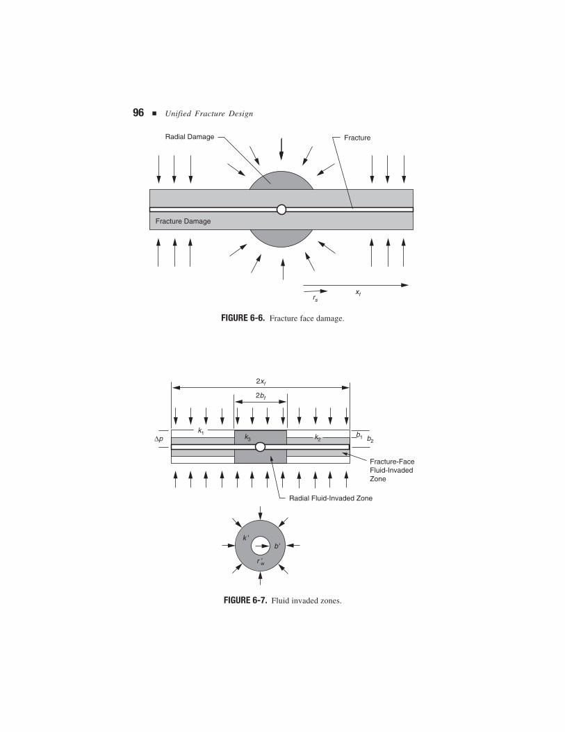
96 ■ Unified Fracture Design
FIGURE 6-6. Fracture face damage.
FIGURE 6-7. Fluid invaded zones.
FractureRadial Damage
rs
xf
Fracture Damage
Radial Fluid-Invaded Zone
Fracture-FaceFluid-InvadedZone
∆p
2xf
2bf
b1 b2k3
k '
k1k2
b'
r 'w
Fracturing Materials ■ 97
in the polymer-invaded zone. A sample of their results (for xf = 25 ft,CfD = 0.1, and kf = 10 md), expressed initially in terms of damagepenetration ratios, b2 /xf , and permeability impairment ratios, k2 /kr , arere-expressed in real units in Table 6-4. Under each of these conditions,the total skin is equal to zero.
These results suggest that for a (nearly impossible) 2.5 ft penetra-tion of damage, a positive skin is obtained only if the permeabilityimpairment in the invaded zone is more than 90 percent. For a damagepenetration of 1.25 ft, the permeability impairment would have to beover 95 percent to achieve positive skins. If the penetration of damagecan be limited to 0.25 ft, even a 99 percent permeability reduction inthe invaded zone would not result in positive skins. At a higherdimensionless conductivity equal to 1, even higher permeability impair-ments can be tolerated without suffering positive skins. Thus, if thefracturing fluid leads to a clean and wide proppant pack, penetrationand damage to the reservoir can be tolerated.
It is also clear from this work that the extent of damage normalto the fracture face is more important than the degree of damage. Iffluid invasion can be minimized, even 99 percent damage can betolerated. The importance of maximizing Cf D is also illustrated; cer-tainly, a good proppant pack should not be sacrificed in an attempt tominimize the fracture face damage.
This points toward the selection of appropriate fracturing fluids:
■ Linear gels by virtue of their considerable leakoff penetrationare not recommended.
■ Crosslinked polymer fluids with high gel loadings appear to bemuch more appropriate.
■ Aggressive breaker schedules are imperative.■ Filter cake building additives may also be considered to mini-
mize the spurt loss and total leakoff.
TABLE 6-4. Fluid Invasion Damage Tolerated for Zero Skin
Depth of Fluid Invasion Permeability Reduction in Normal to Fracture Face Invaded Zone
2.5 ft 90%
1.25 ft 95%
0.25 ft 99%
Source: Aggour and Economides (1996).
98 ■ Unified Fracture Design
Work by Mathur et al. (1995) and Ning et al. (1995) furthersupport the conclusion that fracture face damage should not sig-nificantly alter long-term HPF performance. The Mathur et al. studyof Gulf Coast wells assumed a linear cleanup of the fracture andobserved an improvement of the production rate at early time. TheNing et al. study of gas wells in Alberta, Canada, showed that fractureconductivity has the greatest effect on long-term production rates,whereas the effects of polymer invasion were minimal.
Experiments in Fracturing Fluid Penetration
McGowen et al. (1993) presented a series of experiments showing theextent of fracturing fluid penetration in cores of various permeabilities.Fracturing fluids used were 70 lbm per 1,000-gal HEC and 30 or 40lbm per 1,000 gal borate-crosslinked HPG. Filtrate volumes weremeasured in ml per cm2 of leakoff area (i.e., cm of penetration) fora 10 md limestone and 200 and 1,000 md sandstones at 120°Fand 180°F.
Several conclusions can be drawn from the work:
■ Crosslinked fracturing fluids are far superior to linear gels incontrolling fluid leakoff. For example, 40 lbm per 1,000 galborate-crosslinked HPG greatly outperforms 70 lbm per 1,000gal HEC in 200 md core at 180°F.
■ Linear gel performs satisfactorily in 10 md rock but fails dramati-cally at 200 md. Even aggressive use of fluid loss additives (e.g.,40 lbm per 1,000 gal silica flour) does not appreciably alter theleakoff performance of HEC in 200 md core.
■ Increasing crosslinked gel concentrations from 30 to 40 lbmper 1,000 gal has a major impact on reducing leakoff in200 md core. Crosslinked borate maintains excellent fluid losscontrol in 200 md sandstone and performs satisfactorily even at1,000 md.
This experimental work strongly corroborates the modeling resultsof Aggour and Economides (1996) and points toward the use of higher-concentration crosslinked polymer fluids with, of course, an appro-priately designed breaker system.
Fracturing Materials ■ 99
Viscoelastic Carrier Fluids
HEC and borate-crosslinked HPG fluids are the dominant fluids cur-rently employed in HPF. However, there is a third class of fluid thatdeserves to be mentioned, the so-called viscoelastic surfactant, or VESfluids. There is little debate that these fluids exhibit excellent rheo-logical properties and are non-damaging, even in high permeabilityformations. The elegance of VES fluids is that they do not require theuse of chemical breaker additives; the viscosity of this fluid conve-niently breaks (leaving considerably less residue than polymer-basedfluids) either when it contacts formation oil or condensate or whenits salt concentration is reduced. Brown et al. (1996) present typicalVES fluid performance data and case histories.
The vulnerability of VES fluids is in their temperature limitationand much higher costs per unit volume. The maximum applicationtemperature for VES fluids has only recently been extended from 130°Fup to 240°F.
VES fluids have great potential when considered in a holisticmanner: treatments may cost more than polymer fluids, but the result-ing appropriately sized fracture could be a far superior producer.


Fracture TreatmentDesign7
101
Fracture treatment goes well beyond the sizing of a fracture, as impor-tant as that is for production enhancement, to include the calculationof a pumping schedule that will realize the goals set for the treatment.This chapter also includes discussion of pre-treatment diagnostics thatare often incorporated with fracture treatments to determine or at leastplace bounds on parameters that are critical to the design procedureand execution.
MICROFRACTURE TESTS
The microfracture stress test (“microfrac”) determines the magnitudeof the minimum principal in-situ stress of a target formation. The testusually involves the injection of pressurized fluid into a small, iso-lated zone (4 to 15 ft, 1.2 to 4.6 m) at low injection rates (1 to 25gal/min, 0.010 to 0.095 m3/min). The minimum principal in-situ stresscan be determined from the pressure decline after shut-in or the pres-sure increase at the beginning of an injection cycle. The fracture closurepressure and fracture reopening pressure provide good approximationsfor the minimum principal in-situ stress.
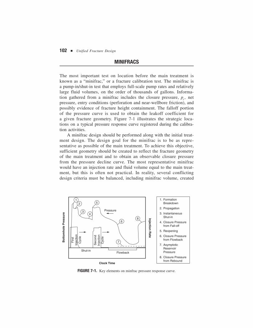
102 ■ Unified Fracture Design
MINIFRACS
The most important test on location before the main treatment isknown as a “minifrac,” or a fracture calibration test. The minifrac isa pump-in/shut-in test that employs full-scale pump rates and relativelylarge fluid volumes, on the order of thousands of gallons. Informa-tion gathered from a minifrac includes the closure pressure, pc , netpressure, entry conditions (perforation and near-wellbore friction), andpossibly evidence of fracture height containment. The falloff portionof the pressure curve is used to obtain the leakoff coefficient fora given fracture geometry. Figure 7-1 illustrates the strategic loca-tions on a typical pressure response curve registered during the calibra-tion activities.
A minifrac design should be performed along with the initial treat-ment design. The design goal for the minifrac is to be as repre-sentative as possible of the main treatment. To achieve this objective,sufficient geometry should be created to reflect the fracture geometryof the main treatment and to obtain an observable closure pressurefrom the pressure decline curve. The most representative minifracwould have an injection rate and fluid volume equal to the main treat-ment, but this is often not practical. In reality, several conflictingdesign criteria must be balanced, including minifrac volume, created
FIGURE 7-1. Key elements on minfrac pressure response curve.
12
34
5
68
7
Pressure
FlowbackShut-in
Firs
tIn
ject
ion
Cyc
le
Sec
ond
Inje
ctio
nC
ycle
Clock Time
Bo
tto
mh
ole
Pre
ssu
re
Injectio
n R
ate
1. FormationBreakdown
2. Propagation
3. InstantaneousShut-in
4. Closure Pressurefrom Fall-off
5. Reopening
6. Closure Pressurefrom Flowback
7. AsymptoticReservoirPressure
8. Closure Pressurefrom Rebound
Fracture Treatment Design ■ 103
fracture geometry, damage to the formation, a reasonable closure time,and the cost of materials and personnel.
Fracture closure is typically determined from one or more con-structions of the pressure decline curve while taking into considerationany available prior knowledge (e.g., that obtained from microfractests). Some of the most popular plots used to identify fracture clo-sure pressure are:
■ pshut-in vs. t
■ pshut-in vs. t
■ pshut-in vs. g-function (and variations)
■ log ( pISIP – pshut-in )
The origin and use of these various plots is sometimes more in-tuitive than theoretical, which can lead to spurious results. The theo-retical basis and limitations of pressure decline analysis must beunderstood in the context of individual applications. An added com-plication is that temperature and compressibility effects may causepressure deviations. In this case, temperature-corrected decline curvescan be generated to permit the normal interpretations of the differentplot types (Soliman, 1984).
The original concept of pressure decline analysis is based on theobservation that the rate of pressure decline during the closure pro-cess contains useful information on the intensity of the leakoffprocess (Nolte, 1979, Soliman and Daneshy, 1991). This stands incontrast to the pumping period, when the pressure is affected by manyother factors.
If we assume that the fracture area has evolved with a constantexponent α and remains constant after the pumps are stopped, at time(te + ∆ t) the volume of the fracture is given by
V = V 2A S 2A g t C tt t i e p e D L ee + − − ( )∆ ∆ ,α (7-1)
where the dimensionless delta time is defined as
∆ ∆t t tD e= / (7-2)
and the two-variable function g(∆tD ,α) can be obtained by integration.Its general form is given by (Valkó and Economides, 1995):
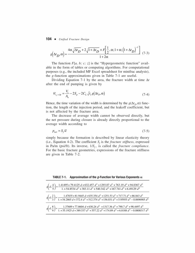
104 ■ Unified Fracture Design
g tD
tD tD F tD∆
∆ ∆ ∆,
, ; ;α
α α α
α( ) =+ + × + +( )
+
−4 2 1
12
1 1
1 2
1
(7-3)
The function F[a, b; c; z] is the “Hypergeometric function” avail-able in the form of tables or computing algorithms. For computationalpurposes (e.g., the included MF Excel spreadsheet for minifrac analysis),the g-function approximations given in Table 7-1 are useful.
Dividing Equation 7-1 by the area, the fracture width at time ∆tafter the end of pumping is given by
e
wV
AS C t g tt t
ip L e De + = − − ( )∆ ∆2 2 ,α (7-4)
Hence, the time variation of the width is determined by the g(∆t D ,α) func-tion, the length of the injection period, and the leakoff coefficient, butis not affected by the fracture area.
The decrease of average width cannot be observed directly, butthe net pressure during closure is already directly proportional to theaverage width according to
p S wnet f= (7-5)
simply because the formation is described by linear elasticity theory(i.e., Equation 4-2). The coefficient Sf is the fracture stiffness, expressedin Pa/m (psi/ft). Its inverse, 1/Sf , is called the fracture compliance.For the basic fracture geometries, expressions of the fracture stiffnessare given in Table 7-2.
TABLE 7-1. Approximation of the g-Function for Various Exponents �
g dd d d d d
d d d d d,45
1 41495 79 4125 632 457 1293 07 763 19 94 03671 54 8534 383 11 540 342 167 741 6 49129
2 3 4 5
2 3 4 5 6
= . + . + . + . + . + .
. + . + . + . + . + .
g dd d d d d
d d d d d d,23
1 47835 81 9445 635 354 1251 53 717 71 86 8431 54 2865 372 4 512 374 156 031 5 95955 0 0696905
2 3 4 5
2 3 4 5 6
=
−. + . + . + . + . + .
.+ . + . + . + . + . .
g dd d d d d
d d d d d d,89
1 37689 77 8604 630 24 1317 36 790 7 98 44971 55 1925 389 537 557 22 174 89 6 8188 0 0808317
2 3 4 5
2 3 4 5 6
=
−. + . + . + . + . + .
.+ . + . + . + . + . .

Fracture Treatment Design ■ 105
TABLE 7-2. Proportionality Constant, Sf and Suggested� for Basic Fracture Geometries
PKN KGD Radial
Sf
2 ′Ehfπ
′Ex fπ
316
π ′ERf
α 4/5 2/3 8/9
The combination of Equations 7-4 and 7-5 yields the following(Nolte, 1979):
p pS V
AS S S C t g tC
f i
ef p f L e D= + −
− ( ) × ( )2 2 ∆ ,α (7-6)
Equation 7-6 shows that the pressure falloff in the shut-in periodwill follow a straight line trend,
p b m g tN N D= − × ( )∆ ,α (7-7)
if plotted against the g-function (i.e., transformed time, Castillo, 1987).The g-function values should be generated with the exponent α con-sidered valid for the given model. The slope of the straight line, mN ,is related to the unknown leakoff coefficient by
Cm
t sLN
e f
= −2 (7-8)
Substituting the relevant expression for fracture stiffness, theleakoff coefficient can be estimated as given in Table 7-3. This tableshows that the estimated leakoff coefficient for the PKN geometry doesnot depend on unknown quantities because the pumping time, frac-ture height, and plain strain modulus are assumed to be known. Forthe other two geometries considered, the procedure results in an esti-mate of the leakoff coefficient that is strongly dependent on the frac-ture extent (xf or Rf ).
From Equation 7-6 we see that the effect of the spurt loss is con-centrated in the intercept of the straight line with the g = 0 axis:
2
SV
A
b p
Spi
e
N C
f
= − −2 (7-9)
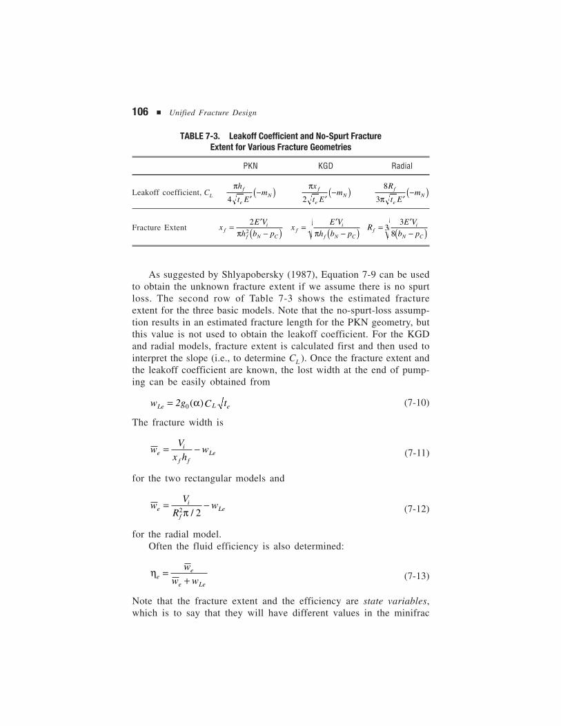
106 ■ Unified Fracture Design
As suggested by Shlyapobersky (1987), Equation 7-9 can be usedto obtain the unknown fracture extent if we assume there is no spurtloss. The second row of Table 7-3 shows the estimated fractureextent for the three basic models. Note that the no-spurt-loss assump-tion results in an estimated fracture length for the PKN geometry, butthis value is not used to obtain the leakoff coefficient. For the KGDand radial models, fracture extent is calculated first and then used tointerpret the slope (i.e., to determine CL ). Once the fracture extent andthe leakoff coefficient are known, the lost width at the end of pump-ing can be easily obtained from
w 2g C tLe L e= 0 ( )α (7-10)
The fracture width is
wV
x hwe
i
f fLe= − (7-11)
for the two rectangular models and
wV
Rwe
i
fLe= −
2 2π / (7-12)
for the radial model.Often the fluid efficiency is also determined:
ηee
e Le
w
w w=
+ (7-13)
Note that the fracture extent and the efficiency are state variables,which is to say that they will have different values in the minifrac
TABLE 7-3. Leakoff Coefficient and No-Spurt FractureExtent for Various Fracture Geometries
PKN KGD Radial
Leakoff coefficient, CL
πh
t Emf
eN
4 ′−( ) πx
t Emf
eN
2 ′−( ) 8
3
R
t Emf
eNπ ′
−( )
Fracture Extent xE V
h b pfi
f N C
= ′−( )
22π
xE V
h b pfi
f N C
= ′−( )π
RE V
b pfi
N C
= ′−( )
3
83
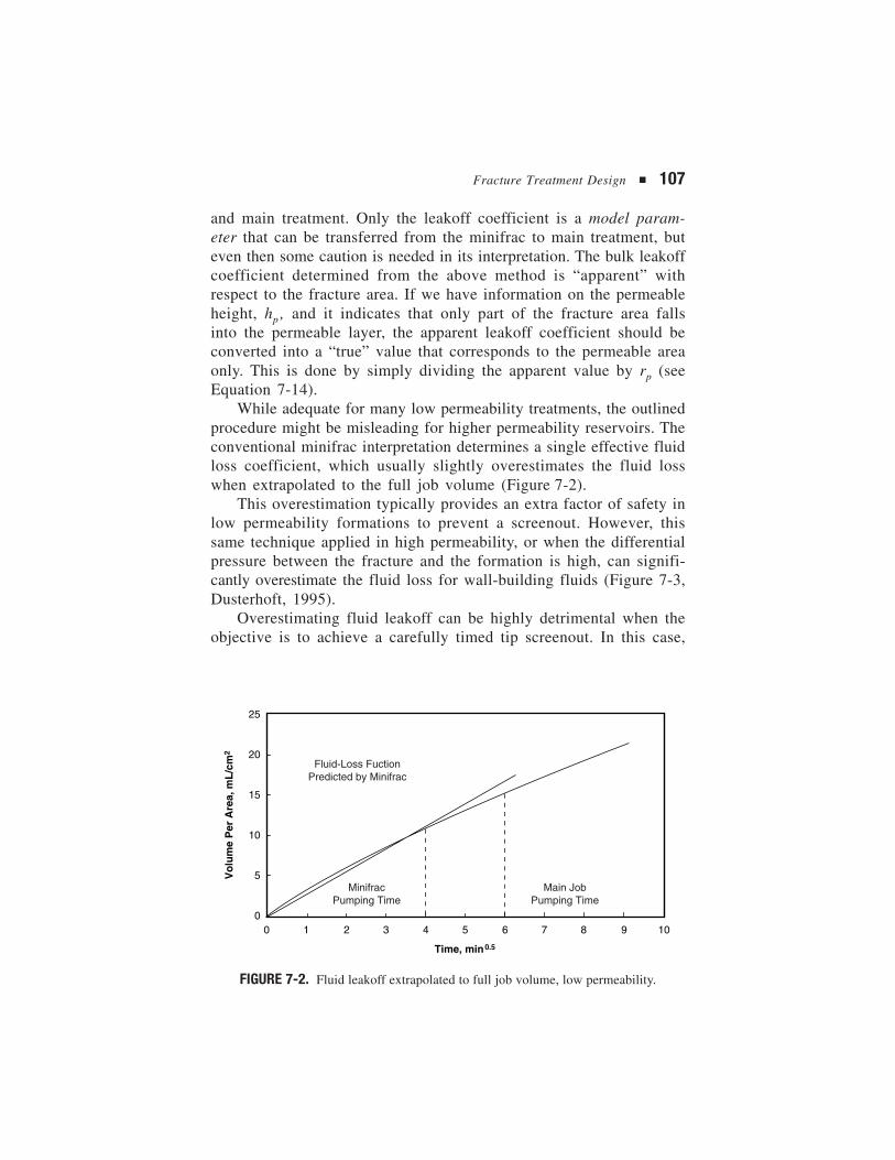
Fracture Treatment Design ■ 107
and main treatment. Only the leakoff coefficient is a model param-eter that can be transferred from the minifrac to main treatment, buteven then some caution is needed in its interpretation. The bulk leakoffcoefficient determined from the above method is “apparent” withrespect to the fracture area. If we have information on the permeableheight, hp , and it indicates that only part of the fracture area fallsinto the permeable layer, the apparent leakoff coefficient should beconverted into a “true” value that corresponds to the permeable areaonly. This is done by simply dividing the apparent value by rp (seeEquation 7-14).
While adequate for many low permeability treatments, the outlinedprocedure might be misleading for higher permeability reservoirs. Theconventional minifrac interpretation determines a single effective fluidloss coefficient, which usually slightly overestimates the fluid losswhen extrapolated to the full job volume (Figure 7-2).
This overestimation typically provides an extra factor of safety inlow permeability formations to prevent a screenout. However, thissame technique applied in high permeability, or when the differentialpressure between the fracture and the formation is high, can signifi-cantly overestimate the fluid loss for wall-building fluids (Figure 7-3,Dusterhoft, 1995).
Overestimating fluid leakoff can be highly detrimental when theobjective is to achieve a carefully timed tip screenout. In this case,
FIGURE 7-2. Fluid leakoff extrapolated to full job volume, low permeability.
25
20
15
10
5
00 1 2 3 4 5 6 7 8 9 10
Time, min0.5
Vo
lum
e P
er A
rea,
mL
/cm
2
Fluid-Loss FuctionPredicted by Minifrac
MinifracPumping Time
Main JobPumping Time
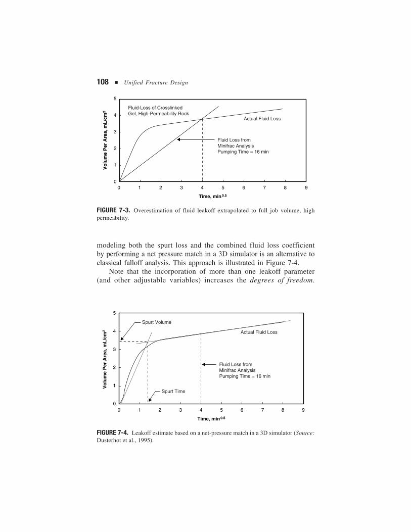
108 ■ Unified Fracture Design
modeling both the spurt loss and the combined fluid loss coefficientby performing a net pressure match in a 3D simulator is an alternative toclassical falloff analysis. This approach is illustrated in Figure 7-4.
Note that the incorporation of more than one leakoff parameter(and other adjustable variables) increases the degrees of freedom.
FIGURE 7-3. Overestimation of fluid leakoff extrapolated to full job volume, highpermeability.
FIGURE 7-4. Leakoff estimate based on a net-pressure match in a 3D simulator (Source:Dusterhot et al., 1995).
5
4
3
2
1
00 1 2 3 4 5 6 7 8 9
Time, min0.5
Vo
lum
e P
er A
rea,
mL
/cm
2Fluid-Loss of CrosslinkedGel, High-Permeability Rock
Fluid Loss fromMinifrac AnalysisPumping Time = 16 min
Actual Fluid Loss
5
4
3
2
1
00 1 2 3 4 5 6 7 8 9
Time, min0.5
Vo
lum
e P
er A
rea,
mL
/cm
2
Spurt Volume
Fluid Loss fromMinifrac AnalysisPumping Time = 16 min
Actual Fluid Loss
Spurt Time
Fracture Treatment Design ■ 109
While a better match of the observed pressure can usually be achieved,the solution often becomes non-unique (i.e., other values of the sameparameters may provide a similar fit).
TREATMENT DESIGN BASED ON THE UNIFIED APPROACH
We ended Chapter 3 by delineating a certain design logic: for a givenamount of proppant reaching the pay layer, we can determine theoptimum length (and width). One of the main results was that, for lowor moderate proppant numbers (relatively low proppant volumes and/ormoderate-to-high formation permeabilities), the optimal compromiseoccurs at CfD = 1.6.
When the formation permeability is above 50 md, it is practicallyimpossible to achieve a proppant number larger than 0.1. Typicalproppant numbers for HPF range from 0.0001 to 0.01. Thus, formoderate and high permeability formations, the optimum dimension-less fracture conductivity is always Cf Dopt = 1.6.
In “tight gas” it is possible to achieve large dimensionless proppantnumbers, at least in principle. If we assume a limited drainage areaand do not question whether the proppant actually reaches the paylayer, a dimensionless proppant number equal to 1 or even 5 can becalculated. However, proppant numbers larger than one are not likelyin practice.
When the propped volume becomes very large, the optimal com-promise happens at larger dimensionless fracture conductivitiessimply because the fracture penetration ratio cannot exceed unity(i.e., fracture length becomes constrained by the well spacing or limitsof the reservoir).
A crucial issue in the design is the assumed fracture height. Therelation of fracture height to pay thickness determines the volumetricproppant efficiency. The actual proppant number depends on that partof the proppant that is placed into the pay. It is calculated as thevolume of injected proppant multiplied by the volumetric proppantefficiency. Therefore, strictly speaking, an optimum target length canbe obtained only if the fracture height is already known. In the fol-lowing, we assume that the fracture height is known. Later we willreturn to this issue.
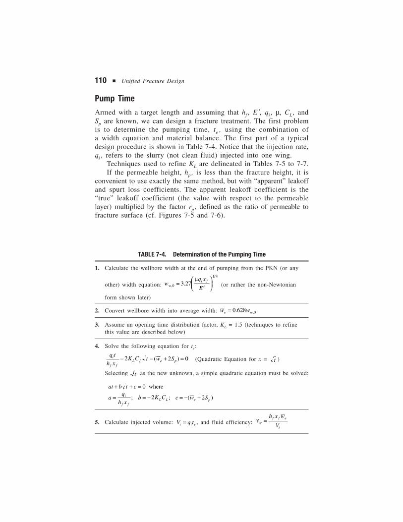
110 ■ Unified Fracture Design
Pump Time
Armed with a target length and assuming that hf , E�, qi , µ, CL , andSp are known, we can design a fracture treatment. The first problemis to determine the pumping time, te , using the combination ofa width equation and material balance. The first part of a typicaldesign procedure is shown in Table 7-4. Notice that the injection rate,qi , refers to the slurry (not clean fluid) injected into one wing.
Techniques used to refine KL are delineated in Tables 7-5 to 7-7.If the permeable height, hp , is less than the fracture height, it is
convenient to use exactly the same method, but with “apparent” leakoffand spurt loss coefficients. The apparent leakoff coefficient is the“true” leakoff coefficient (the value with respect to the permeablelayer) multiplied by the factor rp , defined as the ratio of permeable tofracture surface (cf. Figures 7-5 and 7-6).
TABLE 7-4. Determination of the Pumping Time
1. Calculate the wellbore width at the end of pumping from the PKN (or any
other) width equation: w =
q x
Ewi f
,
/
.0
1 4
3 27µ
′
(or rather the non-Newtonian
form shown later)
2. Convert wellbore width into average width: w we w= 0 628 0. ,
3. Assume an opening time distribution factor, KL = 1.5 (techniques to refinethis value are described below)
4. Solve the following equation for te:
q t
h xK C t w Si
f fLL e p− − + =2 2 0( ) (Quadratic Equation for x = t )
Selecting t as the new unknown, a simple quadratic equation must be solved:
at b t c
aq
h xb K C c w Si
f fLL e p
+ + =
= = − = − +
0
2 2
where
; ; ( )
5. Calculate injected volume: V q ti i e= , and fluid efficiency: ηef f e
i
=h x w
V
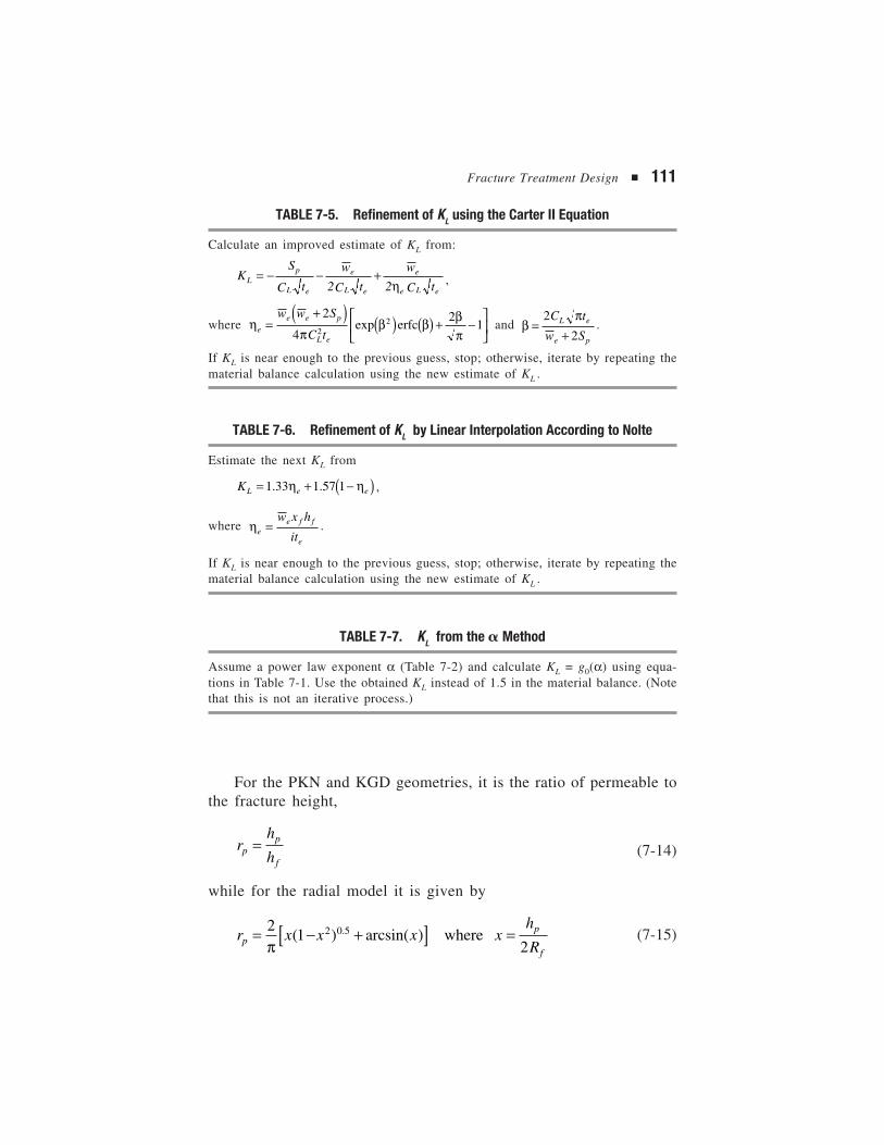
Fracture Treatment Design ■ 111
For the PKN and KGD geometries, it is the ratio of permeable tothe fracture height,
rh
hpp
f
= (7-14)
while for the radial model it is given by
r x x x xh
Rpp
f
= − +[ ] =21
22 0 5
π( ) arcsin( ). where (7-15)
TABLE 7-5. Refinement of KL using the Carter II Equation
Calculate an improved estimate of KL from:
KS
C t
w
2C t
w
2 C tL
p
L e
e
L e
e
e L e
= − − +η ,
where ηπ
β β βπe
e e p
L e
w w S
C t=
+( ) ( ) ( ) + −
2
42
12
2exp erfc and βπ
=+
2
2
C t
w SL e
e p
.
If KL is near enough to the previous guess, stop; otherwise, iterate by repeating thematerial balance calculation using the new estimate of KL .
TABLE 7-6. Refinement of KL by Linear Interpolation According to Nolte
Estimate the next KL from
KL e e= + −( )1 33 1 57 1. .η η ,
where ηee f f
e
w x h
it= .
If KL is near enough to the previous guess, stop; otherwise, iterate by repeating thematerial balance calculation using the new estimate of KL .
TABLE 7-7. KL from the � Method
Assume a power law exponent α (Table 7-2) and calculate KL = g0(α) using equa-tions in Table 7-1. Use the obtained KL instead of 1.5 in the material balance. (Notethat this is not an iterative process.)
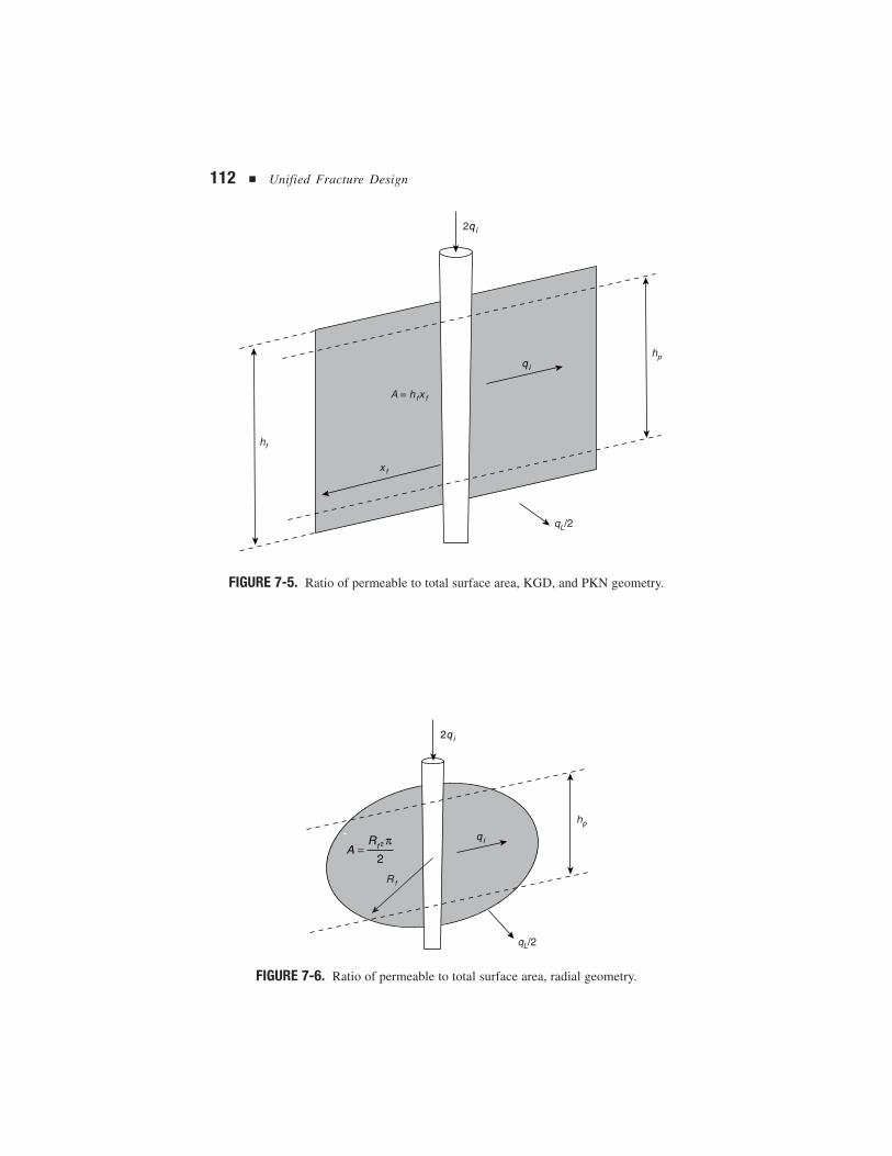
112 ■ Unified Fracture Design
FIGURE 7-5. Ratio of permeable to total surface area, KGD, and PKN geometry.
FIGURE 7-6. Ratio of permeable to total surface area, radial geometry.
hp
qi
qL/2
2qi
Rf
AR
f=2
2
π
2qi
hf
hpq i
x f
A = hfx f
qL/2
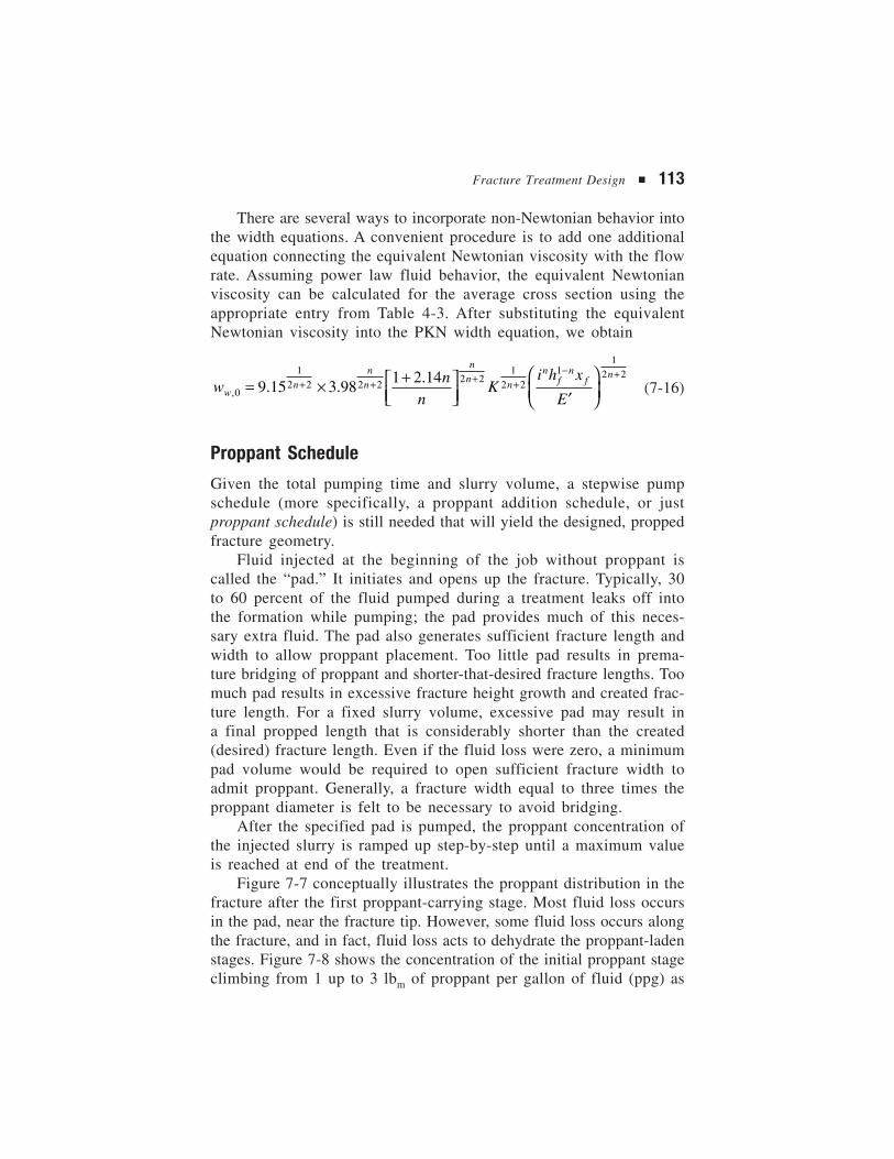
Fracture Treatment Design ■ 113
There are several ways to incorporate non-Newtonian behavior intothe width equations. A convenient procedure is to add one additionalequation connecting the equivalent Newtonian viscosity with the flowrate. Assuming power law fluid behavior, the equivalent Newtonianviscosity can be calculated for the average cross section using theappropriate entry from Table 4-3. After substituting the equivalentNewtonian viscosity into the PKN width equation, we obtain
wn
nK
i h x
Ewn
n
n
n
nn
nf
nf
n
, . ..
0
12 2 2 2
2 21
2 21
12 2
9 15 3 981 2 14= × +
′
+ + + +− +
(7-16)
Proppant Schedule
Given the total pumping time and slurry volume, a stepwise pumpschedule (more specifically, a proppant addition schedule, or justproppant schedule) is still needed that will yield the designed, proppedfracture geometry.
Fluid injected at the beginning of the job without proppant iscalled the “pad.” It initiates and opens up the fracture. Typically, 30to 60 percent of the fluid pumped during a treatment leaks off intothe formation while pumping; the pad provides much of this neces-sary extra fluid. The pad also generates sufficient fracture length andwidth to allow proppant placement. Too little pad results in prema-ture bridging of proppant and shorter-that-desired fracture lengths. Toomuch pad results in excessive fracture height growth and created frac-ture length. For a fixed slurry volume, excessive pad may result ina final propped length that is considerably shorter than the created(desired) fracture length. Even if the fluid loss were zero, a minimumpad volume would be required to open sufficient fracture width toadmit proppant. Generally, a fracture width equal to three times theproppant diameter is felt to be necessary to avoid bridging.
After the specified pad is pumped, the proppant concentration ofthe injected slurry is ramped up step-by-step until a maximum valueis reached at end of the treatment.
Figure 7-7 conceptually illustrates the proppant distribution in thefracture after the first proppant-carrying stage. Most fluid loss occursin the pad, near the fracture tip. However, some fluid loss occurs alongthe fracture, and in fact, fluid loss acts to dehydrate the proppant-ladenstages. Figure 7-8 shows the concentration of the initial proppant stageclimbing from 1 up to 3 lbm of proppant per gallon of fluid (ppg) as
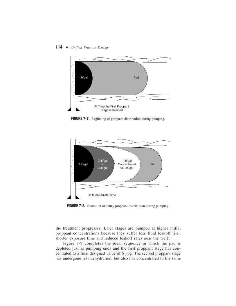
114 ■ Unified Fracture Design
the treatment progresses. Later stages are pumped at higher initialproppant concentrations because they suffer less fluid leakoff (i.e.,shorter exposure time and reduced leakoff rates near the well).
Figure 7-9 completes the ideal sequence in which the pad isdepleted just as pumping ends and the first proppant stage has con-centrated to a final designed value of 5 ppg. The second proppant stagehas undergone less dehydration, but also has concentrated to the same
FIGURE 7-7. Beginning of proppant distribution during pumping.
FIGURE 7-8. Evolution of slurry proppant distribution during pumping.
1 lb/gal Pad
At Time the First ProppantStage is Injected
Pad
At Intermediate Time
3 lb/gal1 lb/gal
Concentratedto 3 lb/gal
2 lb/galto
3 lb/gal
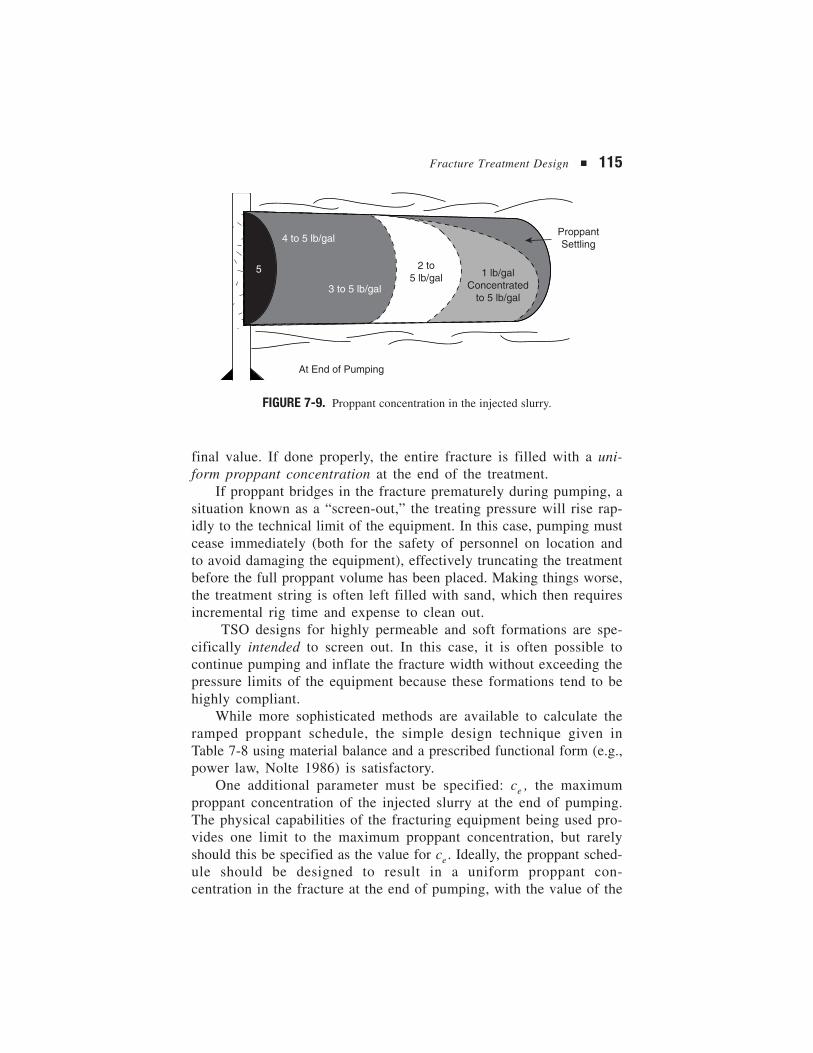
Fracture Treatment Design ■ 115
final value. If done properly, the entire fracture is filled with a uni-form proppant concentration at the end of the treatment.
If proppant bridges in the fracture prematurely during pumping, asituation known as a “screen-out,” the treating pressure will rise rap-idly to the technical limit of the equipment. In this case, pumping mustcease immediately (both for the safety of personnel on location andto avoid damaging the equipment), effectively truncating the treatmentbefore the full proppant volume has been placed. Making things worse,the treatment string is often left filled with sand, which then requiresincremental rig time and expense to clean out.
TSO designs for highly permeable and soft formations are spe-cifically intended to screen out. In this case, it is often possible tocontinue pumping and inflate the fracture width without exceeding thepressure limits of the equipment because these formations tend to behighly compliant.
While more sophisticated methods are available to calculate theramped proppant schedule, the simple design technique given inTable 7-8 using material balance and a prescribed functional form (e.g.,power law, Nolte 1986) is satisfactory.
One additional parameter must be specified: ce , the maximumproppant concentration of the injected slurry at the end of pumping.The physical capabilities of the fracturing equipment being used pro-vides one limit to the maximum proppant concentration, but rarelyshould this be specified as the value for ce . Ideally, the proppant sched-ule should be designed to result in a uniform proppant con-centration in the fracture at the end of pumping, with the value of the
FIGURE 7-9. Proppant concentration in the injected slurry.
At End of Pumping
2 to5 lb/gal
4 to 5 lb/gal
1 lb/galConcentrated
to 5 lb/gal3 to 5 lb/gal
5
ProppantSettling
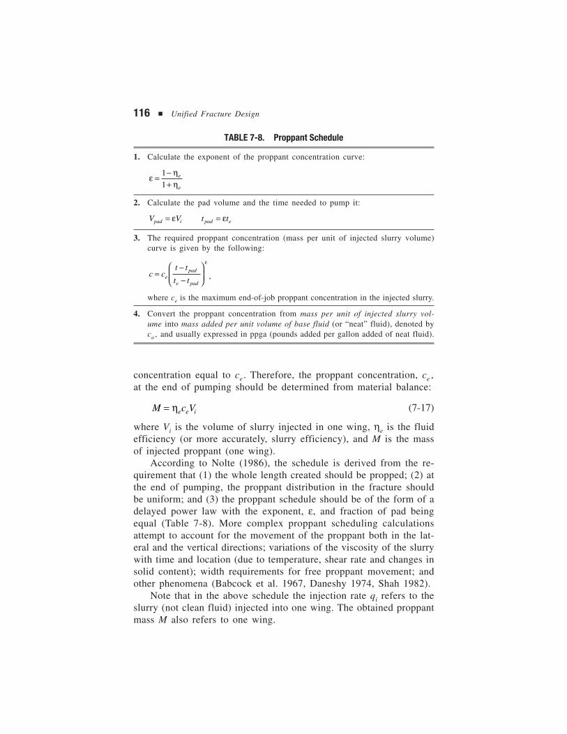
116 ■ Unified Fracture Design
concentration equal to ce . Therefore, the proppant concentration, ce ,at the end of pumping should be determined from material balance:
M c Ve e i= η (7-17)
where Vi is the volume of slurry injected in one wing, ηe is the fluidefficiency (or more accurately, slurry efficiency), and M is the massof injected proppant (one wing).
According to Nolte (1986), the schedule is derived from the re-quirement that (1) the whole length created should be propped; (2) atthe end of pumping, the proppant distribution in the fracture shouldbe uniform; and (3) the proppant schedule should be of the form of adelayed power law with the exponent, ε, and fraction of pad beingequal (Table 7-8). More complex proppant scheduling calculationsattempt to account for the movement of the proppant both in the lat-eral and the vertical directions; variations of the viscosity of the slurrywith time and location (due to temperature, shear rate and changes insolid content); width requirements for free proppant movement; andother phenomena (Babcock et al. 1967, Daneshy 1974, Shah 1982).
Note that in the above schedule the injection rate qi refers to theslurry (not clean fluid) injected into one wing. The obtained proppantmass M also refers to one wing.
TABLE 7-8. Proppant Schedule
1. Calculate the exponent of the proppant concentration curve:
εηη
=−+
1
1e
e
2. Calculate the pad volume and the time needed to pump it:
V Vpad i= ε t tpad e= ε
3. The required proppant concentration (mass per unit of injected slurry volume)curve is given by the following:
c ct t
t tepad
e pad
=−−
ε
,
where ce is the maximum end-of-job proppant concentration in the injected slurry.
4. Convert the proppant concentration from mass per unit of injected slurry vol-ume into mass added per unit volume of base fluid (or “neat” fluid), denoted byca , and usually expressed in ppga (pounds added per gallon added of neat fluid).
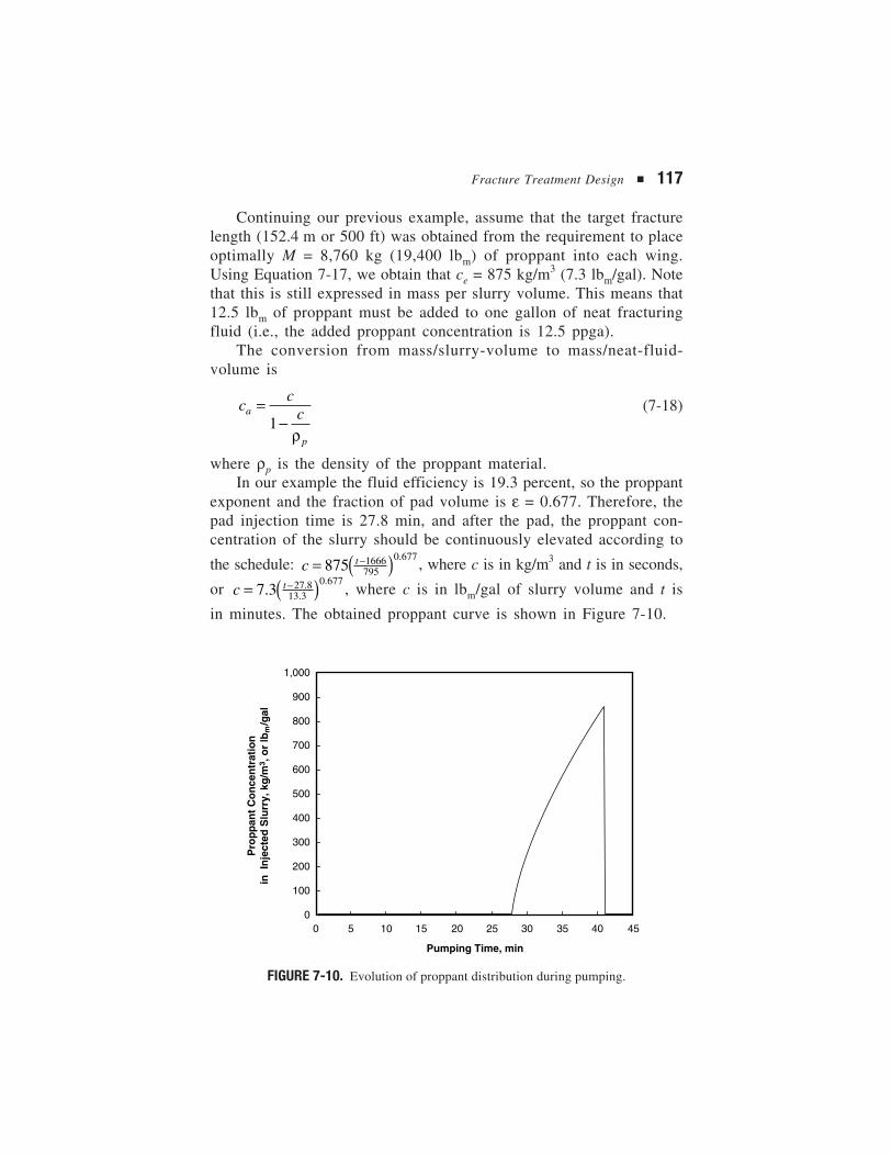
Fracture Treatment Design ■ 117
Continuing our previous example, assume that the target fracturelength (152.4 m or 500 ft) was obtained from the requirement to placeoptimally M = 8,760 kg (19,400 lbm) of proppant into each wing.Using Equation 7-17, we obtain that ce = 875 kg/m3 (7.3 lbm/gal). Notethat this is still expressed in mass per slurry volume. This means that12.5 lbm of proppant must be added to one gallon of neat fracturingfluid (i.e., the added proppant concentration is 12.5 ppga).
The conversion from mass/slurry-volume to mass/neat-fluid-volume is
cc
ca
p
=−1
ρ
(7-18)
where ρp is the density of the proppant material.In our example the fluid efficiency is 19.3 percent, so the proppant
exponent and the fraction of pad volume is ε = 0.677. Therefore, thepad injection time is 27.8 min, and after the pad, the proppant con-centration of the slurry should be continuously elevated according to
the schedule: c t= ( )875 1666795
0 677– ., where c is in kg/m3 and t is in seconds,
or c t= ( )7 3 27 813 3
0 677. – .
.
., where c is in lbm/gal of slurry volume and t is
in minutes. The obtained proppant curve is shown in Figure 7-10.
FIGURE 7-10. Evolution of proppant distribution during pumping.
1,000
900
800
700
600
500
400
300
200
100
00 5 10 15 20 25 30 35 40 45
Pumping Time, min
Pro
pp
ant
Co
nce
ntr
atio
nin
In
ject
ed S
lurr
y, k
g/m
3 , o
r lb
m/g
al
118 ■ Unified Fracture Design
At the end of pumping, the proppant concentration is equal to ce
everywhere in the fracture. Thus, the mass of proppant placed into onewing is M = Ve × ce = ηe × Vi × ce , or in our case, M = 8,760 kg(19,400 lbm). The average propped width after closure can be determinedif the porosity of the proppant bed is known. Assuming φp = 0.3, thepropped volume is Vp = M/[(1 – φp)ρp], or in our case, 6.0 m3. Theaverage propped width is wp = Vp / (xf × hf ), that is, 2 mm (0.078 in.).
A quick check of the dimensionless fracture conductivity, sub-stituting the propped width, shows that CfD = (60 × 10–12 × 0.002)/(5 × 10–16 × 152) = 1.6, as it should be for a treatment with a rela-tively low proppant number.
In the above example, we assumed that the optimum target length andwidth can be realized without any problem. Of course, it is possible thatcertain physical or technical constraints (e.g., maximum possible proppantconcentration in the slurry) do not allow optimal placement.
Departure from the Theoretical Optimum
In case of conflict, the design engineer has several options. One pos-sibility is to overcome technical limitations by, for example, choos-ing another type of fluid, proppant and/or equipment.
More often, however, we choose to depart from the theoreticaloptimum. The art of fracture design is to depart from the theoreticaloptimum dimensions, but in a reasonable manner and only as muchas necessary. In practical terms, this means that the optimum fracturelength or pad volume should be reduced or increased by a “factor.”
For low permeability formations, the first design attempt oftenresults in very long but narrow fracture. Because there is a certainminimum propped width that is required to maintain continuity of thefracture (e.g., 3 times the proppant diameter), the design engineershould reduce the target length—multiplying it by a factor of 0.5or sometimes even 0.1. In a careful design procedure, the engi-neer departs from the theoretical optimum only as much as neces-sary to satisfy another technical limitation, such as a required mini-mum width.
In high permeability formations, the first attempt may result in ashort fracture with insufficient conductivity (width). This portends amove from the conventional to TSO design, which can produce extremelylarge fracture widths.
Fracture Treatment Design ■ 119
TSO Design
It is the tip screenout or TSO design which clearly differentiates highpermeability fracturing from conventional massive hydraulic fractur-ing. While HPF introduces other identifiable differences (e.g., higherpermeability, softer rock, smaller proppant volumes, and so on), it isthe tip screenout that makes these fracturing treatments unique. Con-ventional fracture treatments are designed to propagate laterally andachieve TSO at the end of pumping. In high permeability fracturing,pumping continues beyond the TSO to a second stage of fracture widthinflation and packing. It is this two-stage treatment that gives rise tothe vernacular of frac & pack. The conventional and HPF design con-cepts were illustrated and compared in Figures 5-3 and 5-4.
Early TSO designs commonly called for 50 percent pad (similarto conventional fracturing) and proppant schedules that ramped-up aggressively; then it became increasingly common to reducethe pad to 10 to 15 percent of the treatment and extend the 0.5 to2 lbm/gal stages (which combined may constitute 50 percent of the total slurry volume, for example). Notionally, this was intended to“create width” for the higher concentration proppant addition (e.g., 12to 14 lbm/gal).
In our design model (included HF2D Excel spreadsheet), the TSOdesign procedure differs from the conventional procedure in onebasic feature: it uses a “TSO criterion” to separate the lateral fracturepropagation period from the width inflation period. This criterion isbased on a “dry-to-wet” average width ratio, that is, the ratio of drywidth (assuming only the “dry” proppant is left in the fracture) to wetwidth (dynamically achieved during pumping). According to ourassumptions, the screen-out occurs and arrests fracture propagationwhen the dry-to-wet width ratio reaches a critical value.
After the TSO is triggered, injection of additional slurry onlyserves to inflate the width of the fracture. Thus, it is important toschedule the proppant such that the critical dry-to-wet width ratio isreached at the same time (pumping time) that the created fracturelength matches the optimum fracture length. With the TSO design,practically any width can be achieved—at least in principle. In addi-tion, the first part of any TSO design very much resembles a tradi-tional design, only the target length is reached in a relatively shorttime, and the dry-to-wet width ratio must reach its critical value dur-ing this first part of the treatment.
120 ■ Unified Fracture Design
We suggest a critical dry-to-wet ratio of 0.5 to 0.75 as the TSOcriterion (representing quite dehydrated sand in the fracture). Unfor-tunately, there is no good theoretical or practical method to refine thisvalue. Engineering intuition and previous experience are critical tojudging whether a significant arrest of fracture propagation is evenpossible in a given formation.
There is also no clear procedure to predict if TSO width inflationwill be possible in a given formation, though rock mechanics laboratoryinvestigations can suggest the answer. The formation needs to be “softenough”; in other words, the elasticity modulus cannot be too high.On the other hand, soft formations are often unconsolidated, lackingsignificant cohesion between the formation grain particles. The maintechnical limitation to keep in mind is the net pressure, which increasesduring width inflation. The design engineer should be prepared to departfrom the theoretical optimum placement if necessary to keep the fracturetreating pressure below critical limits imposed by the equipment.
Another consideration in TSO design is that the created fracturemust bypass the assumed damaged region near the wellbore. As such,the design should specify a minimum target length, even if the theoreti-cal optimum calls for a shorter fracture. Often the minimum length ison the order of 50 ft, while the nature of the damage and the lengthof the perforated interval may dictate other values. Note that thisdeparture from the optimum again can be realized by specifyingthe “multiply optimum length by a factor” parameter in the provideddesign software.
PUMPING A TSO TREATMENT
Anecdotal observations related to real-time HPF experiences are abundantin the literature and are not the focus of an engineering-operations textsuch as this. However, some observations related to treatment execu-tion are in order:
■ Most treatments are pumped using a gravel pack service toolin the “circulate” position with the annulus valve closed at thesurface. This allows for live annulus monitoring of bottomholepressure (annulus pressure + annulus hydrostatic head) and real-time monitoring of the progress of the treatment.
Fracture Treatment Design ■ 121
■ When there is no evidence of the planned TSO on the real-timepressure record, the late treatment stages can be pumped at areduced rate to effect a tip screenout. Obviously, this requiresreliable bottomhole pressure data and direct communication bythe frac unit operator.
■ Near the end of the treatment, the pump rate is slowed to gravelpacking rates and the annulus valve is opened to begin circu-lating a gravel pack. The reduced pump rate is maintained untiltubing pressure reaches an upper limit, signaling that the screen-casing annulus is packed.
■ Because very high proppant concentrations are employed, thesand-laden slurry used to pack the screen-casing annulus mustbe displaced from surface with clean gel, well before the endof pumping. Thus, proppant addition and slurry volumes mustbe metered carefully to ensure there is sufficient proppant leftin the tubing to place the gravel pack (i.e., to avoid over-displacing proppant into the fracture).
■ Conversely, if an HPF treatment sands out prematurely (i.e.,with proppant in the tubing), the service tool can be moved intothe “reverse” position and the excess proppant circulated out.
■ Movement of the service tool from the squeeze/circulating posi-tion to the reverse position can create a sharp instantaneousdrawdown effect and should be done carefully to avoid swab-bing unstabilized formation material into the perforation tunnelsand annulus.
Swab Effect Example
The following simple equation, given by Mullen et al. (1994) can beused to convert swab volumes into oilfield unit flow rates:
qV
tss
m
= 2 057, (7-19)
where qs is the instantaneous swab rate in bbl/day, Vs is the swabbedvolume of fluid in gal, tm is the time of tool movement in seconds,and 2,057 is the conversion factor for gal/sec to bbl/day.

122 ■ Unified Fracture Design
The volume of swabbed fluid is calculated from the service tooldiameter and the length of stroke during which the sealed service tooldoes not allow fluid bypass. The average swab volume of a 2.68 in.service tool is 2.8 gal when the service tool is moved from the squeezeposition to the reverse-circulation position. Assuming a rather normalmovement time of 5 sec, this represents an instantaneous productionrate of 1,100 bbl/day.
Perforations for HPF
It is widely agreed that establishing a conductive connection betweenthe fracture and wellbore is critical to the success of HPF, but noconsensus or study has emerged that gives definitive direction.
With an eye toward maximizing conductivity and fluid flow rate,many operators shoot the entire target interval with high shot densityand large holes (e.g., 12 shots per foot with “big hole” charges). Otheroperators—more concerned with multiple fracture initiations, near-welltortuosity, and perforations that are not packed with sand—take theextreme opposite approach, perforating just the middle of the targetinterval with a limited number of 0° or 180° phased perforations.Arguments are made for and against underbalanced versus over-balanced perforating: underbalanced may cause formation failure and“sticking the guns;” overbalanced eliminates a cleanup trip but maynegatively impact the completion efficiency.
Solvent or other scouring pills are commonly circulated to thebottom of the workstring and then reversed out to remove scale, pipedope, or other contaminants prior to pumping into the formation. Sev-eral hundred gallons (e.g., 10 to 25 gallons per foot) of 10 to 15 per-cent HCl acid will then be circulated or bullheaded down to theperforations and be allowed to soak (i.e., to improve communicationwith the reservoir by cleaning up the perforations and dissolvingdebris in the perforation tunnel). Some operators are beginning toforego the solvent and acid cleanup (obviously to reduce rig time andassociated costs). Their presumption is that the damaging materialis pumped deep into the formation and will not seriously impactwell performance.
PRE-TREATMENT DIAGNOSTIC TESTS FOR HPF
There are several features unique to high permeability fracturing whichmake pre-treatment diagnostic tests and well-specific design strategies
Fracture Treatment Design ■ 123
highly desirable if not essential: fracture design in soft formations isvery sensitive to leakoff and net pressure; the controlled nature of thesequential tip screenout/fracture inflation and packing/gravel packingprocess demands relatively precise execution strategies; and the treat-ments are very small and typically “one-shot” opportunities. Further-more, methods used in hard-rock fracturing to determine criticalfracture parameters a priori (e.g., geologic models, log and core data,or Poisson ratio computational models based on poroelasticity) are oflimited value or not yet adapted to the unconsolidated, soft, high per-meability formations.
There are three tests (with variations) that form the current basisof pre-treatment testing in high permeability formations: step-rate tests,minifrac tests, and pressure falloff tests.
Step-Rate Tests
The step-rate test (SRT), as implied by the name, involves injectingclean gel at several stabilized rates, beginning at matrix rates andprogressing to rates above fracture extension pressure. In a high per-meability environment, a test may be conducted at rate steps of 0.5,1, 2, 4, 8, 10, and 12 barrels per minute, and then at the maximumattainable rate. The injection is held steady at each rate step for auniform time interval (typically 2 or 3 minutes at each step).
In principle, the test is intended to identify the fracture extensionpressure and rate. The stabilized pressure (ideally bottomhole pressure)at each step is classically plotted on a Cartesian graph versus injec-tion rate. Two straight lines are drawn, one through those points thatare obviously below the fracture extension pressure (dramatic increasein bottomhole pressure with increasing rate), and a second throughthose points that are clearly above the fracture extension pressure(minimal increase in pressure with increasing rate). The point at whichthe two lines intersect is interpreted as the fracture extension pressure.The dashed lines on Figure 7-11 illustrate this classic approach.
While the conventional SRT is operationally simple and inexpen-sive, it is not necessarily accurate. A Cartesian plot of bottomholepressure versus injection rate, in fact, does not generally form astraight line for radial flow in an unfractured well. Simple pressuretransient analysis of SRT data using desuperposition techniques showsthat with no fracturing the pressure versus rate curve should exhibitupward concavity. Thus, the departure of the real data from idealbehavior may occur at a pressure and rate well below that indicated bythe classic intersection of the straight lines (see Figure 7-11).
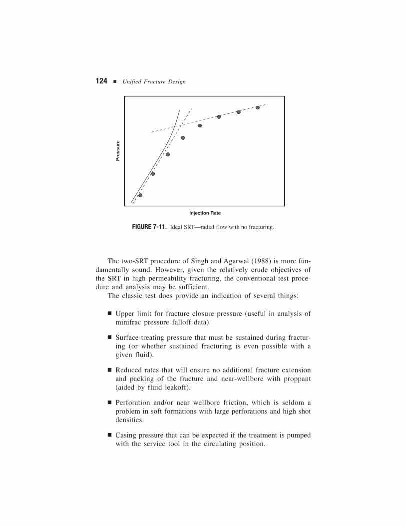
124 ■ Unified Fracture Design
The two-SRT procedure of Singh and Agarwal (1988) is more fun-damentally sound. However, given the relatively crude objectives ofthe SRT in high permeability fracturing, the conventional test proce-dure and analysis may be sufficient.
The classic test does provide an indication of several things:
■ Upper limit for fracture closure pressure (useful in analysis ofminifrac pressure falloff data).
■ Surface treating pressure that must be sustained during fractur-ing (or whether sustained fracturing is even possible with agiven fluid).
■ Reduced rates that will ensure no additional fracture extensionand packing of the fracture and near-wellbore with proppant(aided by fluid leakoff).
■ Perforation and/or near wellbore friction, which is seldom aproblem in soft formations with large perforations and high shotdensities.
■ Casing pressure that can be expected if the treatment is pumpedwith the service tool in the circulating position.
FIGURE 7-11. Ideal SRT—radial flow with no fracturing.
Injection Rate
Pre
ssu
re
Fracture Treatment Design ■ 125
A step-down option to the normal SRT is sometimes used specificallyto identify near-wellbore restrictions (tortuosity or perforation friction).This test is done immediately following a minifrac or other pump-instage. By observing bottomhole pressure variations with decreasingrate, near-wellbore restrictions can be immediately detected (i.e.,bottomhole pressures that change only gradually as injection rate isreduced sharply in steps is indicative of no restriction).
Minifracs
Following the SRT, a minifrac should be performed to tailor the HPFtreatment with well-specific information. This is the critical diagnos-tic test. The minifrac analysis and treatment design modifications cantypically be done on-site in less than an hour.
Concurrent with the rise of HPF, minifrac tests, and especially theuse of bottomhole pressure information, have become much morecommon. Otherwise, the classic minifrac procedure and primary out-puts as described in the preceding section (i.e., determination of frac-ture closure pressure and a bulk leakoff coefficient) are widely appliedto HPF, this in spite of some rather obvious shortcomings.
The selection of closure pressure, a difficult enough task in hardrock fracturing, can be arbitrary or nearly impossible in high permeabil-ity, high-fluid-loss formations. In some cases, the duration of the clo-sure period is so limited (one minute or less) that the pressure signalis masked by transient phenomena. Deviated wellbores and laminatedformations (common in offshore U.S. Gulf Coast completions), multiplefracture closures, and other complex features are often evident duringthe pressure falloff. The softness of these formations (i.e., low elasticmodulus) means very subtle fracture closure signatures on the pres-sure decline curve. Flowbacks are not used to accent closure featuresbecause of the high leakoff and concerns with production of uncon-solidated formation sand.
New guidelines and diagnostic plots for determining closure pres-sure in high-permeability formations are being pursued by variouspractitioners and will eventually emerge to complement or replace thestandard analysis and plots.
The shortcomings of classic minifrac analysis are further exposedwhen used (commonly) to select a single effective fluid loss coeffi-cient for the treatment. As described above, in low permeability for-mations this approach results in a slight overestimation of fluid lossand actually provides a factor of safety to prevent screenout. In high
126 ■ Unified Fracture Design
permeability formations, the classic approach can dramatically under-estimate spurt loss (zero spurt loss assumption) and overestimatetotal fluid loss. This uncertainty in leakoff behavior makes the con-trolled timing of a tip screenout very difficult. Entirely new proce-dures based on sound fundamentals of leakoff in HPF (as outlined inChapter 5) are ultimately needed. The traditional practice of account-ing for leakoff with a bulk leakoff coefficient is simply not sufficientfor this application.
Pressure Falloff Tests
A third class of pre-treatment diagnostics for HPF has emerged thatis not common to MHF: pressure falloff tests. Owing to the high for-mation permeability, common availability of high quality bottom-hole pressure data, and multiple pumping and shut-in cycles, matrixformation properties including kh and skin can be determined fromshort duration pressure falloff tests using the appropriate transient flowequation. Chapman et al. (1996) and Barree et al. (1996) propose pre-frac or matrix injection/falloff tests that involve injecting completionfluid below fracturing rates for a given period of time, and then ana-lyzing the pressure decline using a Horner plot.
The test is performed using standard pumping equipment and poseslittle interruption to normal operations. A test can normally be com-pleted within one hour or may even make use of data from unplannedinjection/shut-in cycles.
The resulting permeability certainly relates to fluid leakoff asdescribed in Chapter 5 and allows the engineer to better anticipatefluid requirements. An initial skin value is useful in “benchmarking”the HPF treatment and for comparison with post-treatment pressuretransient analysis.
Bottomhole Pressure Measurements
A discussion of pre-treatment diagnostic tests requires a discussion ofthe source of pressures used in the analysis. Implicit to the discus-sion is that the only meaningful pressures are those adjacent to thefracture face, whether measured directly or translated to that point.There are at least four different types of bottomhole pressure data,depending on the location at which the real data are taken:
Fracture Treatment Design ■ 127
■ Calculated bottomhole pressure—implies bottomhole pressurecalculated from surface pumping pressure.
■ Deadstring pressure—open annulus, bottomhole pressure deducedknowing density of fluid in annulus; tubing may also be used asdead string when treatment is pumped down the casing.
■ Bundle carriers in the workstring—measured downhole, but abovethe service tool crossover.
■ Washpipe data—attached to washpipe below service tool crossover.
Washpipe pressure data is the most desirable for HPF design andanalysis based on its location adjacent to the fracture and downstreamof all significant flowing pressure drops. Workstring bundle carrier datacan introduce serious error in many cases because of fluid frictiongenerated through the crossover tool and in the casing-screen annu-lus. Without detailed friction pressure corrections that account forspecific tool dimensions and annular clearance, there is a possibilityfor a significant departure between washpipe and workstring bundlecarrier pressures. Deadstring pressures are widely used and consideredacceptable by most practitioners; some others suggest that redundantwashpipe pressure data has shown that the deadstring can mask subtlefeatures of the treatment. The use of bottomhole transducers with real-time surface readouts is suggested in cases where a dead string is notfeasible or when well conditions (e.g., transients) may obscure impor-tant information.
Reliance on bottomhole pressures calculated from surface pump-ing pressure is not recommended in HPF. The combination of heavysand-laden fluids, constantly changing proppant concentrations, veryhigh pump rates, and short pump times makes the estimation of fric-tion pressures nearly impossible.