Embed Size (px)
Citation preview
8/10/2019 Joshi Priyanka
http://slidepdf.com/reader/full/joshi-priyanka 1/166
i
Effect of Pre-treatment using Ultrasound and Hydrogen Peroxide
on Digestion of Waste Activated Sludge in an
Anaerobic Membrane Bioreactor
by
Priyanka Dilip Joshi
A thesis
presented to the University of Waterloo
in fulfillment of the
thesis requirement for the degree of
Master of Applied Science
in
Civil Engineering
Waterloo, Ontario, Canada, 2014
© Priyanka Dilip Joshi 2014

8/10/2019 Joshi Priyanka
http://slidepdf.com/reader/full/joshi-priyanka 2/166
ii
Author’s Declaration
I hereby declare that I am the sole author of this thesis. This is a true copy of the thesis, including
any required final revisions, as accepted by my examiners. I understand that my thesis may be
made electronically available to the public.
8/10/2019 Joshi Priyanka
http://slidepdf.com/reader/full/joshi-priyanka 3/166
iii
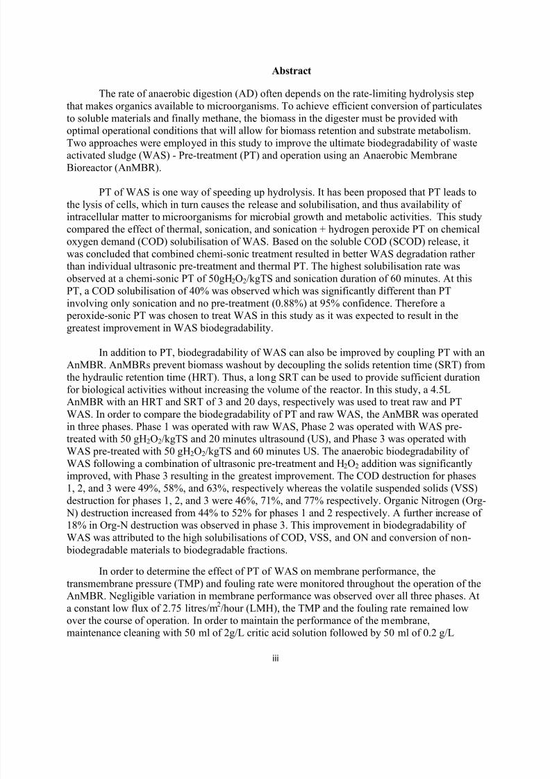
Abstract
The rate of anaerobic digestion (AD) often depends on the rate-limiting hydrolysis step
that makes organics available to microorganisms. To achieve efficient conversion of particulates
to soluble materials and finally methane, the biomass in the digester must be provided withoptimal operational conditions that will allow for biomass retention and substrate metabolism.
Two approaches were employed in this study to improve the ultimate biodegradability of waste
activated sludge (WAS) - Pre-treatment (PT) and operation using an Anaerobic Membrane
Bioreactor (AnMBR).
PT of WAS is one way of speeding up hydrolysis. It has been proposed that PT leads to
the lysis of cells, which in turn causes the release and solubilisation, and thus availability ofintracellular matter to microorganisms for microbial growth and metabolic activities. This study
compared the effect of thermal, sonication, and sonication + hydrogen peroxide PT on chemical
oxygen demand (COD) solubilisation of WAS. Based on the soluble COD (SCOD) release, it
was concluded that combined chemi-sonic treatment resulted in better WAS degradation ratherthan individual ultrasonic pre-treatment and thermal PT. The highest solubilisation rate was
observed at a chemi-sonic PT of 50gH2O2/kgTS and sonication duration of 60 minutes. At this
PT, a COD solubilisation of 40% was observed which was significantly different than PT
involving only sonication and no pre-treatment (0.88%) at 95% confidence. Therefore a peroxide-sonic PT was chosen to treat WAS in this study as it was expected to result in the
greatest improvement in WAS biodegradability.
In addition to PT, biodegradability of WAS can also be improved by coupling PT with an
AnMBR. AnMBRs prevent biomass washout by decoupling the solids retention time (SRT) from
the hydraulic retention time (HRT). Thus, a long SRT can be used to provide sufficient duration
for biological activities without increasing the volume of the reactor. In this study, a 4.5LAnMBR with an HRT and SRT of 3 and 20 days, respectively was used to treat raw and PT
WAS. In order to compare the biodegradability of PT and raw WAS, the AnMBR was operated
in three phases. Phase 1 was operated with raw WAS, Phase 2 was operated with WAS pre-treated with 50 gH2O2/kgTS and 20 minutes ultrasound (US), and Phase 3 was operated with
WAS pre-treated with 50 gH2O2/kgTS and 60 minutes US. The anaerobic biodegradability of
WAS following a combination of ultrasonic pre-treatment and H2O2 addition was significantlyimproved, with Phase 3 resulting in the greatest improvement. The COD destruction for phases
1, 2, and 3 were 49%, 58%, and 63%, respectively whereas the volatile suspended solids (VSS)
destruction for phases 1, 2, and 3 were 46%, 71%, and 77% respectively. Organic Nitrogen (Org-
N) destruction increased from 44% to 52% for phases 1 and 2 respectively. A further increase of18% in Org-N destruction was observed in phase 3. This improvement in biodegradability of
WAS was attributed to the high solubilisations of COD, VSS, and ON and conversion of non-
biodegradable materials to biodegradable fractions.
In order to determine the effect of PT of WAS on membrane performance, the
transmembrane pressure (TMP) and fouling rate were monitored throughout the operation of theAnMBR. Negligible variation in membrane performance was observed over all three phases. At
a constant low flux of 2.75 litres/m2/hour (LMH), the TMP and the fouling rate remained low
over the course of operation. In order to maintain the performance of the membrane,maintenance cleaning with 50 ml of 2g/L critic acid solution followed by 50 ml of 0.2 g/L
8/10/2019 Joshi Priyanka
http://slidepdf.com/reader/full/joshi-priyanka 4/166
iv
sodium hypochlorite was performed three times a week. In addition, a gas sparing rate of 2
L/minute and a permeation cycle of 10 minutes with 8 minutes of operation followed by 2
minutes of relaxation was employed. During phase 2 of this study, a new membrane wasinstalled due to a faulty gas sparging pump. A slight decrease of TMP was observed with the
installation of the new membrane; however the decrease was minimal. In addition critical flux
for phases 2 and 3 were determined to be in the range of 6 to 12 LMH.
In conclusion, the incorporation of H2O2-US PT with AD could allow treatment plants to
substantially reduce the mass flow of solids and organics and thus result in a decrease in
requirements for downstream sludge processing. With sufficient maintenance, steady operationcould be achieved for a hollow fibre AnMBR with a total solids concentration range of 20-25
g/L, an HRT of 3 days, and an SRT of 20 days. It was found that PT could be successfully
integrated with AnMBR to substantially reduce the HRT required for digestion when compared
to conventional designs.
8/10/2019 Joshi Priyanka
http://slidepdf.com/reader/full/joshi-priyanka 5/166
v
Acknowledgements
Many people have played a role in supporting and guiding me through this degree.
Firstly, I would like to thank Dr. Wayne Parker for his guidance and expertise, without
which I wouldn’t have been able to complete this degree. I am extremely grateful to him for
taking the time out of his busy schedule, meeting with me every time I needed his help, and
promptly replying to all my e-mails. I consider myself very lucky to have worked with such a
knowledgeable and respectable person.
I am also grateful to GE Wastewater for supplying equipment for this study and to
Martha Dagnew and Kyle Walder at the Wastewater Technology Centre (WTC) for being patient
with me and answering my questions while I was acquainting myself with all the equipment and
processes.
I would also like to extend my gratefulness and thanks to my fellow lab mates –
Mohammed Galib, Hyeongu Yu, Yaohuan Gao, Hou Yu, and Qiaosi Deng for sharing the lab
space and equipment with me and assisting me in lab work. I am also thankful to Mark Merlau,
Mark Sobon, Tom Sullivan and Terry Ridgeway for their assistance in trips to the WWTP and
WTC and troubleshooting lab equipment. I am appreciative of Gillian Staples Burger and
Peiman Kianmehr for replying to my e-mails promptly and answering my questions on lab
equipment and procedures.
Last but not least, I am deeply grateful to my family and friends for their support and
love. Their words of encouragement kept me going through tough times and my study.
8/10/2019 Joshi Priyanka
http://slidepdf.com/reader/full/joshi-priyanka 6/166
vi
Table of Contents
Author’s Declaration .............................................................................................................................. ii
Abstract .................................................................................................................................................. iii
Acknowledgments .................................................................................................................................. v
Table of Contents ................................................................................................................................... vi
List of Figures ........................................................................................................................................ xi
List of Tables ........................................................................................................................................ xiii
List of Abbreviations ............................................................................................................................ xiv
1.
Introduction ..................................................................................................................................... 1
1.1. Problem Statement ................................................................................................................... 2
1.2. Objectives ................................................................................................................................ 2
1.3. Thesis Structure ....................................................................................................................... 3
2. Literature Review ............................................................................................................................ 4
2.1. Introduction ............................................................................................................................. 4
2.2.
Anaerobic Digestion ................................................................................................................ 4
2.3. Anaerobic Biological Treatment Process ................................................................................ 5
2.4. Anaerobic Membrane Bioreactor ............................................................................................ 7
2.5. Anaerobic Digestion of High Solids Waste using AnMBRs ................................................... 7
2.6. Membrane Performance of AnMBR systems treating High Solids Waste ............................. 12
2.6.1. Fouling in AnMBRs ....................................................................................................... 12
2.6.2. Conceptual Model of Fouling Mechanisms ................................................................... 12
2.6.3. Prevention and Control of Fouling ................................................................................. 15
2.6.4.
Studies on Membrane Performance of AnMBR systems treating High Solids Waste .. 16

8/10/2019 Joshi Priyanka
http://slidepdf.com/reader/full/joshi-priyanka 7/166
vii
2.7. WAS Pre-treatment................................................................................................................. 22
2.8. Ultrasonic Pre-treatment ......................................................................................................... 23
2.9. Chemical Pre-treatment .......................................................................................................... 28
2.10.
Combined Peroxide-Ultrasonic Pre-treatment ........................................................................ 30
2.11. Integration of Pre-treatment and AnMBRs ............................................................................. 32
2.12. Summary of Chapter 2 ............................................................................................................ 34
3. Pre-treatment of WAS .................................................................................................................... 36
3.1.
Introduction ............................................................................................................................ 36
3.2. Materials and Methods ........................................................................................................... 43
3.2.1.
Waste Activated Sludge Characteristics ........................................................................ 43
3.2.2.
Pre-treatment Conditions ............................................................................................... 44
3.2.2.1. Sonication Pre-treatment ..................................................................................... 44
3.2.2.2. Pre-treatment using Hydrogen Peroxide/Ultrasound ........................................... 45
3.2.2.3. Thermal Pre-treatment ......................................................................................... 45
3.2.3. Anaerobic Membrane Bioreactor Digestion Operations ................................................ 47
3.2.4.
Operation of AnMBR .................................................................................................... 49
3.2.5. Sampling Protocol .......................................................................................................... 50
3.2.5.1. Feed Collection .................................................................................................... 51
3.2.5.2.
PT of WAS .......................................................................................................... 51
3.2.5.3. AnMBR Monitoring ............................................................................................ 51
3.2.6. Sample Analysis ............................................................................................................. 52
3.2.6.1.
Total COD .......................................................................................................... 53
3.2.6.2. Soluble COD ....................................................................................................... 53
3.2.6.3. Flocculated and Filtered COD ............................................................................. 54
3.2.6.4. Ammonia ............................................................................................................. 54
3.2.6.5. Total Kjeldahl Nitrogen ....................................................................................... 54
8/10/2019 Joshi Priyanka
http://slidepdf.com/reader/full/joshi-priyanka 8/166
viii
3.2.6.6. Soluble TKN ........................................................................................................ 55
3.2.6.7. Nitrate .................................................................................................................. 55
3.2.6.8. Suspended Solids ................................................................................................. 55
3.2.6.9.
Volatile Fatty Acids to Alkalinity Ratio .............................................................. 56
3.2.6.10. pH ...................................................................................................................... 56
3.3. Results and Discussion ........................................................................................................... 56
3.3.1. Preliminary Pre-treatment Tests ..................................................................................... 56
3.3.2.
Detailed Pre-treatment Tests .......................................................................................... 62
3.3.2.1. Impact of Peroxide-Sonic PT on Physio-chemical Characteristics of WAS ....... 62
3.3.2.1.1.
COD Comparison ...................................................................................... 62
3.3.2.1.2.
Suspended Solids ....................................................................................... 65
3.3.2.1.3. Nitrogen Species ....................................................................................... 67
3.3.3. Anaerobic Membrane Bioreactor Operation ................................................................. 71
3.3.3.1. pH and VFA/Alk Ratio for AnMBR ................................................................... 71
3.3.3.2. COD Destruction and Analysis ........................................................................... 74
3.3.3.3.
Solids Destruction ............................................................................................... 80
3.3.3.4. Organic Nitrogen Destruction and Analysis ........................................................ 84
3.3.3.5. COD Decay Tests – Estimation of Biodegradable COD ..................................... 91
3.3.4.
Comparison of Phases .................................................................................................... 93
3.4. Conclusion ……………………………………………………………………………………94
4. Membrane Performance of AnMBR treating WAS ....................................................................... 96
4.1.
Introduction ............................................................................................................................ 96
4.2. Materials and Methods .......................................................................................................... 100
4.2.1. Experimental Set-up ...................................................................................................... 100
4.2.2. Operational Conditions ................................................................................................. 101
4.2.3. Membrane Cleaning Procedure ...................................................................................... 101
8/10/2019 Joshi Priyanka
http://slidepdf.com/reader/full/joshi-priyanka 9/166
ix
4.2.4. Critical Flux Determination ........................................................................................... 102
4.2.5. Sample Analysis ............................................................................................................ 102
4.3. Results ................................................................................................................................... 103
4.3.1.
Overall Membrane Performance .................................................................................... 103
4.3.2. Impact of Solids Fractions on Membrane Performance ................................................ 107
4.3.3. Impact of COD Fractions on Membrane Performance ................................................. 108
4.3.4. Critical Flux Test ........................................................................................................... 109
4.4.
Conclusion ........................................................................................................................... 112
5. Conclusions ................................................................................................................................... 113
5.1.
Comparison of Pre-treatments – Preliminary Tests ............................................................... 113
5.2.
Comparison of the 20 and 60 minutes US AOP – Detailed Tests ......................................... 114
5.2.1. Physico-chemical Comparison of the 20 and 60 minutes US AOP .............................. 114
5.2.2. Biodegradability Comparison of the 20 and 60 minutes US AOP ................................ 115
5.3. Membrane Performance of AnMBR ..................................................................................... 116
6. Recommendations ......................................................................................................................... 117
6.1.
Pre-treatment and AnMBR Biodegradation Operations ........................................................ 117
6.2. Membrane Operations ........................................................................................................... 117
References ............................................................................................................................................ 119
Appendix A: Physio-Chemical, Biodegradation and Membrane Operations Data .............................. 133
Appendix A1: Factorial Design for US + H2O2 AOP .......................................................................... 133
Appendix A2: Statistical Analysis t-tests............................................................................................. 134
Appendix A3: Preliminary PT Tests .................................................................................................... 140
Appendix A4: Detailed PT 8 Tests ...................................................................................................... 141
Appendix A5: Detailed PT 10 Tests .................................................................................................... 143
Appendix A6: COD Destruction Results ............................................................................................. 145
Appendix A7: Solids Destruction Results ........................................................................................... 146
8/10/2019 Joshi Priyanka
http://slidepdf.com/reader/full/joshi-priyanka 10/166
x
Appendix A8: ON Destruction Results ................................................................................................ 147
Appendix A9: COD Decay Tests for Phase 2 and Phase 3 .................................................................. 148
Appendix 10: Critical Flux Tests for Phase 2 and Phase ..................................................................... 149
8/10/2019 Joshi Priyanka
http://slidepdf.com/reader/full/joshi-priyanka 11/166
xi
List of Figures
Figure 2.1: Biological Description of Anaerobic Digestion .................................................................. 6
Figure 3.1: Ultrasound Flow Through System...................................................................................... 45
Figure 3.2: Thermal Pre-treatment Process Flow ................................................................................. 46
Figure 3.3: Overview of Experimental Plan ......................................................................................... 48
Figure 3.4: AnMBR Process Flow Diagram ......................................................................................... 49
Figure 3.5: Fractionation of COD employed in this study .................................................................... 53
Figure 3.6: Fractionation of COD for all PTs ....................................................................................... 57
Figure 3.7: Average COD Concentration in Raw and Pre-treated Samples ......................................... 63
Figure 3.8: Suspended Solids Concentration for Detailed AOP Testing .............................................. 66
Figure 3.9: Nitrogen Species Concentration in Raw and Pre-treated WAS .......................................... 67
Figure 3.10: Impact of 20 and 60 US minutes AOP on ON/COD ratios .............................................. 70
Figure 3.11: pH in AnMBR throughout all Phases ............................................................................... 72
Figure 3.12: VFA/Alk in AnMBR throughout all Phases ..................................................................... 74
Figure 3.13: Total COD destruction for Phase 1 Steady State .............................................................. 75
Figure 3.14: COD Destructions Rates for Phase 1, 2, and 3 ................................................................. 75
Figure 3.15: Average COD Concentrations in Phase 1, 2, and 3 AnMBR WAS ................................. 77
Figure 3.16: Cumulative Mass Balance of COD species through PT and AD ..................................... 79
Figure 3.17: Average Permeate ffCOD concentrations for all Phases .................................................. 80
Figure 3.18: Total VSS destruction for Phase 1 Steady State ............................................................... 81
Figure 3.19: VSS Destruction Rates for Phase 1, 2, and 3 .................................................................... 82
Figure 3.20: Average SS Concentrations in Phase 1, 2, and 3 AnMBR WAS ..................................... 84
Figure 3.21: Total ON destruction for Phase 1 Steady State ................................................................ 85
Figure 3.22: ON Destruction Rates for Phase 1, 2, and 3 ..................................................................... 86
Figure 3.23: Average Nitrogen Concentrations in Phase 1, 2, and 3 AnMBR WAS ........................... 88
Figure 3.24: Cumulative TKN Mass Balance in Phase 1, 2, and 3 ....................................................... 90
8/10/2019 Joshi Priyanka
http://slidepdf.com/reader/full/joshi-priyanka 12/166
xii
Figure 3.25: Average Ammonia Concentrations in Phase 1, 2, and 3 Permeate .................................. 90
Figure 3.25: COD Decay Results for Phase 2 and Phase 3 ................................................................... 93
Figure 3.26: Total COD, VSS, and ON Destruction Rates for all Phases ............................................ 94
Figure 4.1: Overall Membrane Performance of Digested Sludge ........................................................ 105
Figure 4.2: Fouling Rate Observed Throughout Membrane Operation ............................................... 107
Figure 4.3: Effect of Solids Loading on Membrane Fouling ............................................................... 108
Figure 4.4: Effect of Colloidal COD on Membrane Fouling ............................................................... 109
Figure 4.5: Critical Flux Test Results .................................................................................................. 110
Figure 4.6: Critical Flux Range for Phase 2 and Phase 3..................................................................... 111
Figure A6.1: Phase 2 COD Destruction ............................................................................................... 144
Figure A6.2: Phase 3 COD Destruction ............................................................................................... 144
Figure A7.1: Phase 2 Solids Destruction ............................................................................................. 145
Figure A7.2: Phase 2 Solids Destruction ............................................................................................. 145
Figure A8.1: ON Destruction for Phase 2 ............................................................................................ 146
Figure A8.2: ON Destruction for Phase 3 ............................................................................................ 146
8/10/2019 Joshi Priyanka
http://slidepdf.com/reader/full/joshi-priyanka 13/166
xiii
List of Tables
Table 2.1: Advantages and Disadvantages of Anaerobic Digestion ...................................................... 5
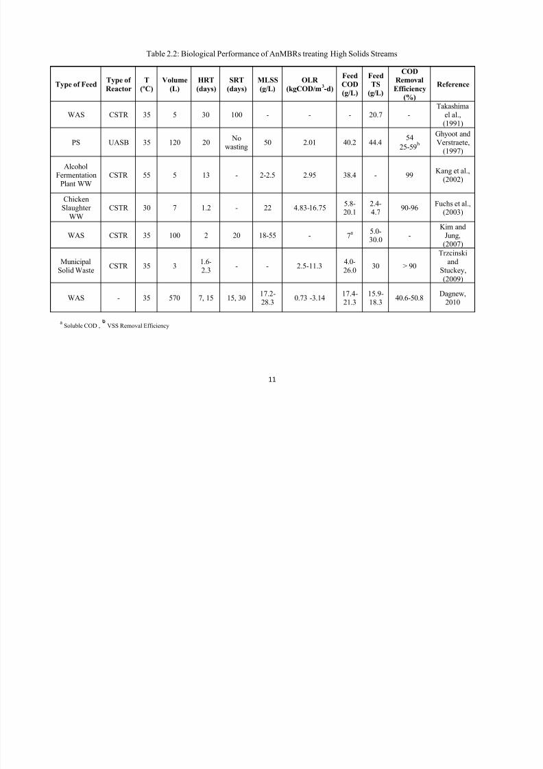
Table 2.2: Biological Performance of AnMBRs treating High Solids Streams .................................... 11
Table 2.3: Classical Membrane Fouling Models .................................................................................. 14
Table 2.4: Membrane Performance of AnMBRs treating High Solids Streams ................................... 21
Table 2.5: Summary of Literature on Sonication Effects on WAS ....................................................... 27
Table 3.1: Characteristics of Thickened WAS ...................................................................................... 43
Table 3.2: PT Conditions ...................................................................................................................... 46
Table 3.3: AnMBR Operation Timeline ............................................................................................... 50
Table 3.4: Sampling Schedule .............................................................................................................. 52
Table 4.1: Steady State Operational Conditions Relevant for Membrane Performance ...................... 101
Table A1.1: 2 x 4 Factorial Design for US + H 2O2 PT ........................................................................ 133
Table A3.1: Preliminary PT Results .................................................................................................... 140
Table A4.1: Detailed Tests for PT 8 RAW .......................................................................................... 141
Table A4.2: Detailed Tests for PT 8 WAS .......................................................................................... 141
Table A4.3: Detailed Solids Tests for PT 8 WAS ............................................................................... 142
Table A5.1: Detailed Tests for PT 10 RAW ........................................................................................ 143
Table A5.2: Detailed Tests for PT 10 WAS ........................................................................................ 143
Table A5.3: Detailed Solids Tests for PT 10 ....................................................................................... 144
Table A9.1: COD Decay Data for Phase 2 .......................................................................................... 148
Table A9.2: COD Decay Data for Phase 3 .......................................................................................... 148
Table A10.1: Critical Flux Test for Phase 2 ........................................................................................ 149
Table A10.2: Critical Flux Test for Phase 3 ........................................................................................ 149
8/10/2019 Joshi Priyanka
http://slidepdf.com/reader/full/joshi-priyanka 14/166
xiv
List of Abbreviations
AD: Anaerobic Digestion
AOT: Advanced Oxidation Treatment
AOP: Advance Oxidation Process
AnMBR: Anaerobic Membrane Bioreactor
cCOD: Colloidal Chemical Oxygen Demand
COD: Chemical Oxygen Demand
CSTR: Continuous Stirred-Tank Reactor
DS: Dry Solids
EPS: Extracellular Polymeric Substances
ffCOD: Flocculated and Filtered COD
FSS: Fixed Suspended Solids
GC: Gas Chromatograph
HRT: Hydraulic Residence Time
ISS: Inert Suspended Solids
LMH: Litre/meter square/hour
MBR: Membrane Bioreactor
MLSS: Mixed Liquor Suspended Solids
MF: Microfiltration
MW: Microwave
OLR: Organic Loading Rate
ON: Organic Nitrogen
P: Permeate
PAN: Polyacrylonitrile
pCOD: Particulate Chemical Oxygen Demand
PDVF: Polyvinylidene Flouride
8/10/2019 Joshi Priyanka
http://slidepdf.com/reader/full/joshi-priyanka 15/166
xv
PE: Polyethylene
PES: Polyethersulfone
PSF: Polusulfone
P1: Phase 1
P2: Phase 2
P3: Phase 3
PS: Primary Sludge
PT: Pre-treatment
PVDF: Polyvinylidene fluoride
SMP: Soluble Microbial Products
sON: Soluble Organic Nitrogen
SCOD: Soluble Chemical Oxygen Demand
SCOD/TCOD: Solubilisation Ratio
SRT: Solids Residence Time
SS: Suspended Solids
sTKN: Soluble Total Kjeldahl Nitrogen
TCD: Thermal Conductivity Detector
TKN: Total Kjeldahl Nitrogen
TMP: Transmembrane Pressure
tON: Total Organic Nitrogen
TWAS: Thickened Waste Activated Sludge
TS: Total Solids
TSS: Total Suspended Solids
UASB: Upflow Anaerobic Sludge Blanket
UF: Ultrafiltration
US: Ultrasound
8/10/2019 Joshi Priyanka
http://slidepdf.com/reader/full/joshi-priyanka 16/166
xvi
VFA/Alk: Volatile Acids to Alkalinity Ratio
VS: Volatile Solids
VSS: Volatile Suspended Solids
W: Waste
WAS: Waste Activated Sludge
WW: Waste Water
WWTP: Waste Water Treatment Plant
8/10/2019 Joshi Priyanka
http://slidepdf.com/reader/full/joshi-priyanka 17/166
1
Chapter 1: Introduction
1.1. Problem Statement
Typically, there are two types of sludge that are generated at wastewater treatment plants
(WWTPs) – Primary (PS) and Waste Activated Sludge (WAS). Primary sludge is a product of
the sedimentation of raw wastewaters while the activated sludge process is responsible for
producing large quantities of waste activated sludge (WAS). A popular means of treating excess
sludge is to stabilize the sludge by anaerobic digestion (AD). AD reduces the organic content and
pathogenic population of WAS while producing methane as a renewable by-product. This
process accomplishes stabilisation of sludge in 4 stages: Hydrolysis, Acidogenesis,
Acetogenesis, and Methanogenesis. It has been established that the rate of hydrolysis is often the
rate limiting step (Bougrier et al., 2006). In order to accommodate this slow process, anaerobic
digesters need to be operated at long solid retention times (SRT), which results in an increase in
reactor volumes due to an increase in the hydraulic retention time (HRT). Several approaches
have been introduced to improve the rate of hydrolysis, which may result in a decrease in reactor
volumes and associated costs.
Pre-treatment (PT) of sludge has been found to be one way of increasing the rate of
hydrolysis (Shahriari et al., 2011). Pre-treatment causes the lysis of cells, thus making organics
and nutrients readily available for microbial growth and metabolic activities. A wide range of
WAS pre-treatments such as thermal (Bougrier et al., 2006; Climent et al., 2007; Bravo et al.,
2011; and Burger, 2012), chemical such as peroxidation (Grönroos et al., 2004; Dewil et al.,
2007; Eskicioglu et al., 2008; and Song et al., 2012), and mechanical such as sonication (Salsabil
et al., 2009; Yan et al., 2010; Kim et al., 2010; Braguglia et al., 2011; and Yaqci et al., 2011)
have been proven to be effective in pre-treating sludge.
8/10/2019 Joshi Priyanka
http://slidepdf.com/reader/full/joshi-priyanka 18/166
2
Another method to enhance the process of anaerobic digestion is to incorporate a
membrane into the design of the digester. With an anaerobic membrane bioreactor (AnMBR),
the solids retention time (SRT) can be decoupled from the hydraulic residence time (HRT), thus
allowing operation at higher loadings and producing digested sludge with higher solids
concentrations while occupying less space in the WWTP. Although AnMBRs appear to provide
considerable advantages over conventional digesters when bioreactor performance is considered,
a potential challenge is the fouling of membranes due to the accumulation of microorganisms,
colloids, solutes, and cell debris in or on membrane surfaces (Meng el al., 2009). Thus
identification of foulants and fouling mechanisms and incorporation of fouling minimization
techniques are required for successful AnMBR operation.
Although AnMBRs may increase the rate of organics destruction the improvement in
extent of biodegradation may be limited by the maximum biodegradability of the feed sludge.
The integration of PT with AnMBRs may provide a solution by increasing the ultimate
biodegradability of WAS. With a significant amount of particulates broken down due to PT, a
high sludge age and the use of membranes to prevent biomass washout may result in an
enhanced destruction of compounds.
This study evaluated a combined PT-AnMBR system to improve the ultimate
biodegradability of WAS. Thermal, ultrasound (US), and peroxide/US treatments were initially
compared to determine the preferred method to enhance the biodegradability of the WAS used in
this study. Once the preferred PT was determined, it was evaluated in tandem with AD in a
submerged hollow fibre AnMBR to allow for a longer SRT while keeping the HRT at a
minimum duration.
8/10/2019 Joshi Priyanka
http://slidepdf.com/reader/full/joshi-priyanka 19/166
3
1.2. Objectives
The objectives of this research were to:
Assess the impact of thermal, sonication, and sonication-peroxide pre-treatments on the
physico-chemical properties of WAS.
Examine the biological performance (COD, solids, and organic nitrogen destruction) of a
low pressure and low shear velocity hollow fibre anaerobic membrane bioreactor in
combination with pre-treatment.
Examine the membrane performance (fouling, impact of colloids and inerts
concentration, flux and transmembrane pressure) of a low pressure and low shear velocity
hollow fibre anaerobic membrane bioreactor in combination with pre-treatment.
1.3. Thesis Structure
This thesis is organized into 6 chapters and 10 appendices. Chapter 1 provides a short
introduction to current WAS stabilization processes, WAS pre-treatment procedures, advantages
and limitations of AnMBRs and outlines the objectives of the study. Chapter 2 summarizes the
literature on previous studies relevant to this study including those that evaluated the effect of PT
on high solids waste streams, digestion of high solids waste streams via AnMBRs and the effect
of high solids waste streams on membrane fouling. Chapter 3 presents the methodology
employed and the results of testing that evaluated the effect of PT on the physico-chemical
properties of WAS and the biological performance of a combined PT-AnMBR system. Chapter 4
presents the methodology employed and the results obtained in a study of the membrane
performance of the AnMBR when treating raw and pre-treated WAS. Chapter 5 presents the
significant conclusions of this study while Chapter 6 provides recommendations for future work.
8/10/2019 Joshi Priyanka
http://slidepdf.com/reader/full/joshi-priyanka 20/166
4
Chapter 2: Literature Review
2.1. Introduction
Typically, there are two types of sludge that are generated at wastewater treatment plants
(WWTPs) – Primary (PS) and Waste Activated Sludge (WAS). Primary sludge is a product of
the sedimentation of raw wastewaters while WAS is a product of biological processes such as the
activated sludge process. With growing populations the amount of sludge to be treated at
WWTPs is increasing. This poses a challenge to WWTP owners and operators since the costs
associated with sludge processing may be as high as 50% of the total cost of wastewater
treatment (Zhang et al., 2007). In this study, sludge stabilization by anaerobic digestion was
evaluated.
2.2. Anaerobic Digestion:
Anaerobic digestion (AD) is a common sludge stabilization method employed in
wastewater treatment plants that not only converts the organic matter into a renewable source of
energy i.e. biogas, but also decreases the amount of solids while destroying a majority of the
pathogens in the sludge (Abelleira et al., 2012). This complex biochemical process employs
several groups of facultative and anaerobic microorganisms that work together to achieve
stabilization and treatment of sludge in the absence of oxygen. The advantages and
disadvantages of AD are summarized in Table 2.1.

8/10/2019 Joshi Priyanka
http://slidepdf.com/reader/full/joshi-priyanka 21/166
5
Table 2.1: Advantages and Disadvantages of Anaerobic Digestion
Advantages Disadvantages
No oxygen required- lower energy
required than aerobic digestion
Low biosolids produced than aerobic
digestion – decrease in sludge
processing and disposal costs
Methane produced as a by-product –
renewable source of energy
High organic loading possible
Low nutrient requirements than aerobic
digestion
Slower process than aerobic digestion –
low growth rate of microorganisms
More sensitive to toxins than aerobic
digestion
More susceptible to low temperatures
than aerobic digestion
May require alkalinity addition
Produces odours
Source: Maier et al., 2008 and Metcalf and Eddy, 2003
2.3. Anaerobic Biological Treatment Process:
Anaerobic processes decompose organic matter in 4 stages: Hydrolysis, acidogenesis,
acetogenesis, and methanogenesis. In hydrolysis, complex molecules such as insoluble organic
matter and high molecular weight compounds are broken down into soluble monomers such as
amino acids, sugars, and fatty acids by a variety of hydrolytic bacteria. Since this is a relatively
slow process, it is typically the rate limiting step in anaerobic digestion of waste activated sludge
(Bougrier et al., 2006). Hydrolysis is followed by acidogenesis that converts monomers into
organic acids, alcohols, ketones, carbon-dioxide, and hydrogen by fermentative acidogenic
bacteria. Acidogenesis is followed by acetogenesis that involves the conversion of acids and
8/10/2019 Joshi Priyanka
http://slidepdf.com/reader/full/joshi-priyanka 22/166
6
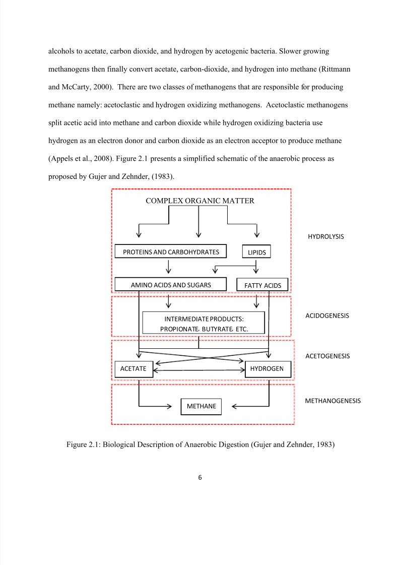
alcohols to acetate, carbon dioxide, and hydrogen by acetogenic bacteria. Slower growing
methanogens then finally convert acetate, carbon-dioxide, and hydrogen into methane (Rittmann
and McCarty, 2000). There are two classes of methanogens that are responsible for producing
methane namely: acetoclastic and hydrogen oxidizing methanogens. Acetoclastic methanogens
split acetic acid into methane and carbon dioxide while hydrogen oxidizing bacteria use
hydrogen as an electron donor and carbon dioxide as an electron acceptor to produce methane
(Appels et al., 2008). Figure 2.1 presents a simplified schematic of the anaerobic process as
proposed by Gujer and Zehnder, (1983).
COMPLEX ORGANIC MATTER
Figure 2.1: Biological Description of Anaerobic Digestion (Gujer and Zehnder, 1983)
PROTEINS AND CARBOHYDRATES LIPIDS
AMINO ACIDS AND SUGARS FATTY ACIDS
INTERMEDIATE PRODUCTS:
PROPIONATE BUTYRATE ETC.
ACETATE HYDROGEN
METHANE
HYDROLYSIS
ACETOGENESIS
ACIDOGENESIS
METHANOGENESIS
8/10/2019 Joshi Priyanka
http://slidepdf.com/reader/full/joshi-priyanka 23/166
7
2.4. Anaerobic Membrane Bioreactors
As stated earlier, hydrolysis is often the rate limiting step in anaerobic digestion
(Bougrier et al., 2006). In addition, due to the slow growth rates of methanogens, conventional
anaerobic digesters need to be operated at long residence times (Dagnew, 2010). One major
drawback of operating digesters at long residence times is that the volume of the reactors are
large, which in turn increases the costs associated with the construction and maintenance of the
digester. Collectively, these factors act to increase the cost of conventional digestion.
One way to enhance the process of anaerobic digestion is to incorporate a membrane into
the design of the digester (Pickel, 2010). With an anaerobic membrane bioreactor (AnMBR), the
solids retention time (SRT) can be decoupled from the hydraulic residence time (HRT), thus
resulting in the ability to treat high loadings and sludge with high solids concentrations and
slowly biodegradable compounds while occupying less space in the WWTP. The membrane is
able to retain the biomass and microorganisms in the digester also resulting in a waste effluent
with high solids concentration. Moreover, the permeate that is collected as a result of the
membrane installation is solids-free (Lew et al., 2009). Due to all these advantages, AnMBRs are
gaining popularity in the waste water industry.
2.5. Anaerobic Digestion of High Solids Waste using AnMBRs
Table 2.2 presents a cross-section of research that has been conducted to evaluate
treatment of high solids streams using AnMBRs. As it can be seen in the table, AnMBRs have
been operated under a variety of different conditions. Conventional anaerobic digesters are
usually operated at a minimum HRT and SRT of 15 days for sludges (Metcalf and Eddy, 2003).
The AnMBR literature has made use of HRTs that have ranged from 1.2 to 30 days (Fuchs et al.,
8/10/2019 Joshi Priyanka
http://slidepdf.com/reader/full/joshi-priyanka 24/166
8
2003 and Takashima et al., 1991). However, when compared to the corresponding decoupled
SRTs (range of 20 days to 365 days), it can be seen that the HRT values were considerably lower
than the SRT, thus demonstrating a low reactor volume (Kim and Jung, 2007 and Ghyoot and
Verstraete, 1997). Comparatively, long SRTs indicate that longer durations may be required to
accomplish significant hydrolysis of high solids streams.
Some studies have evaluated the influence of SRT on chemical oxygen demand (COD)
and volatile suspended solids (VSS) destruction rates. For instance, Dagnew, (2010) investigated
the effect of SRT on the performance of a submerged AnMBR treating WAS and found that as
the SRT was increased from 15 to 30 days, the VSS and COD destruction rates increased from
36 ± 1.5 % to 48.6 ± 3.1% and from 40.6 ± 1.8 % to 50.8 ± 3.8%, respectively. Trzcinski and
Stuckey, (2010) also investigated the effect of SRT on COD removal rates of a submerged
AnMBR treating municipal solid waste leachate and found that as SRT increased from 30 to 300
days, the fraction of removed COD also increased. It was seen that as the SRT increases,
microorganisms are able to hydrolyze particulates and high molecular weight molecules into
smaller and soluble substances more effectively. Hence, microorganisms are able to degrade
COD and VSS more effectively. Most of the studies discussed in Table 2.2 reported that
decoupling SRT-HRT in AnMBRs kept the volume of the reactor low while accomplishing
significant digestion of the high solids streams as shown by the high destructions.
Another operational parameter that is commonly reported in the operation of anaerobic
reactors is the organic loading rate (OLR). Puchajda and Oleszkiewicz, (2008) have shown that
increasing the loading rate can enhance anaerobic digestion. However, in order to ensure
successful anaerobic digestion, conventional digesters are usually operated at high SRTs (and
thus HRTs), which may result in low OLRs. This was confirmed by Verstraete and Vandevivere
8/10/2019 Joshi Priyanka
http://slidepdf.com/reader/full/joshi-priyanka 25/166
9
(1999) found that conventional anaerobic digesters are usually operated at low OLRs of < 1
kgCOD/m3/d. On the other hand, due to the decoupling SRT-HRT characteristic of AnMBRs,
these systems are expected to be able to handle high OLRs. The applied OLR for AnMBRs was
higher than 1 kg COD/m3/d in the studies listed in Table 2.2, and in some cases higher than
10 kg COD/m3/d, demonstrating the capacity of AnMBRs to handle high loadings (Fuchs et al.,
2003 and Trzcinski and Stuckey, 2009).
However, despite the potential improvement in sustainability, using high loadings may
negatively affect the AnMBR process. This is because high OLRs may require high cross flow
velocities or sparging rates and more cleaning to prevent fouling of the membrane. Some studies
have reported a decline in digester performance at high OLRs (Brockmann and Seyfried, 1997;
Hernandez et al., 2002; and Padmasiri et al., 2007). This deterioration in performance was
attributed to a decline in microbial activity as a result of high shear rates and physical
interruption of the syntrophic interaction of acetogenic and methanogenic organisms
(Brockmann and Seyfried, 1997 and Hernandez et al., 2002). Therefore, shear rates that are
adequate enough to accomplish scouring of membranes and do not affect the biological activity
of microorganisms should be employed.
Temperature is another factor that affects the activity of microorganisms. It should be
noted that most of the studies reported in this review evaluated mesophilic reactors, with the
exception of the study of Kang et al., (2002), where the AnMBR was operated at a thermophilic
temperature of 55ºC. This shows that a broad range of temperatures can be employed in
AnMBRs. From a biological point of view, microbial growth and decay rates have been reported
to be linearly related to temperature (Dereli et al., 2012). The higher decay rate of thermophilic
bacteria may lead to the formation of small particles such as extracellular polymeric substances
8/10/2019 Joshi Priyanka
http://slidepdf.com/reader/full/joshi-priyanka 26/166
10
(EPS), decay products or cell debris (Dereli et al., 2012). The existence of such particles within
the reactor may have a negative effect on the filtration properties of the membrane, a concern
that will be addressed in Section 2.5.
In some cases, similar removal efficiencies have been reported with thermophilic and
mesophilic AnMBRs. For instance, Kang et al., (2002) reported a 99% COD removal efficiency
at 55ºC, while Fuchs et al., (2003) observed a 90-96% removal efficiency by operating the
reactor at only 30ºC. However, both studies employed AnMBRs to treat different waste streams
under different operational conditions. Kang et al., (2002) operated the AnMBR at an HRT of 13
days and OLR of 2.95 kg COD/m3/d to treat an alcohol fermentation plant WW with an MLSS
concentration of 2-2.5 g/L, while Fuchs et al., (2003) used an HRT of 1.2 days and OLR of 4.83-
16.75 kg COD/m3/d to treat 22 gMLSS/L chicken slaughter WW. Despite having a higher MLSS
concentration and OLR, Kang et al., (2002) achieved a high removal rate, which was comparable
to Fuchs et al., (2003). Therefore, in order to minimize costs of heating, one may operate
AnMBRs at mesophilic temperatures and acquire high removal efficiencies that one would
observe at thermophilic temperatures.
In summary, the literature reveals that AnMBRs can be operated over a broad range of
conditions; however the removal efficiency that can be maintained is a function of sludge
characteristics, shear rate, and operational conditions. On the basis of the reviewed literature, the
test apparatus employed in this study was designed to operate at a low HRT, a comparatively
higher SRT, an OLR > 1 kgCOD/m3/d and a mesophilic temperature. This combination of
operational conditions was chosen to accomplish a high removal rate while maintaining the costs
at a minimum.
8/10/2019 Joshi Priyanka
http://slidepdf.com/reader/full/joshi-priyanka 27/166
11
Table 2.2: Biological Performance of AnMBRs treating High Solids Streams
Type of FeedType of
Reactor
T
(ºC)
Volume
(L)
HRT
(days)
SRT
(days)
MLSS
(g/L)
OLR
(kgCOD/m3-d)
Feed
COD
(g/L)
Feed
TS
(g/L)
COD
Removal
Efficiency(%)
Reference
WAS CSTR 35 5 30 100 - - - 20.7 -Takashima
el al.,(1991)
PS UASB 35 120 20 No
wasting50 2.01 40.2 44.4
54
25-59 b
Ghyoot andVerstraete,
(1997)
AlcoholFermentation
Plant WWCSTR 55 5 13 - 2-2.5 2.95 38.4 - 99
Kang et al.,(2002)
ChickenSlaughter
WW
CSTR 30 7 1.2 - 22 4.83-16.755.8-20.1
2.4-4.7
90-96Fuchs et al.,
(2003)
WAS CSTR 35 100 2 20 18-55 - 7a
5.0-30.0
-Kim and
Jung,(2007)
Municipal
Solid Waste CSTR 35 3
1.6-
2.3 - - 2.5-11.3
4.0-
26.0 30 > 90
Trzcinskiand
Stuckey,(2009)
WAS - 35 570 7, 15 15, 3017.2-28.3
0.73 -3.1417.4-21.3
15.9-18.3
40.6-50.8Dagnew,
2010
aSoluble COD , VSS Removal Efficiency
8/10/2019 Joshi Priyanka
http://slidepdf.com/reader/full/joshi-priyanka 28/166
12
2.6. Membrane Performance of AnMBR systems treating High Solids Waste
2.6.1. Fouling in AnMBR
Although AnMBRs appear to provide considerable advantages over conventional
digesters when bioreactor performance is considered, a potential challenge is the fouling of
membranes due to the accumulation of microorganisms, colloids, solutes, and cell debris in or on
membrane surfaces (Meng el al., 2009). Fouling is an unavoidable drawback of using a
membrane as it affects the long term stability and performance of the membrane. Inefficient
operation of membranes due to fouling will require elevated energy costs and may require
frequent replacement of membranes, which in turn increases costs (Dereli et al., 2012).
In order to study fouling it is desirable to have metrics that can be used to quantify its
extent. Two indicators of fouling have been reported in literature. It has been described in terms
of either an increase in transmembrane pressure (TMP) (at constant flux) or a decrease in flux (at
constant TMP) (Hong et al., 2002). Most studies on membrane fouling have used a constant flux
approach rather than a constant TMP approach (Choi, 2003). Defrance and Jaffrin, (1999)
confirmed that it is preferable to operate the membrane at a constant flux rather than at a constant
TMP. Hence, the AnMBR in this study was operated in a constant flux mode.
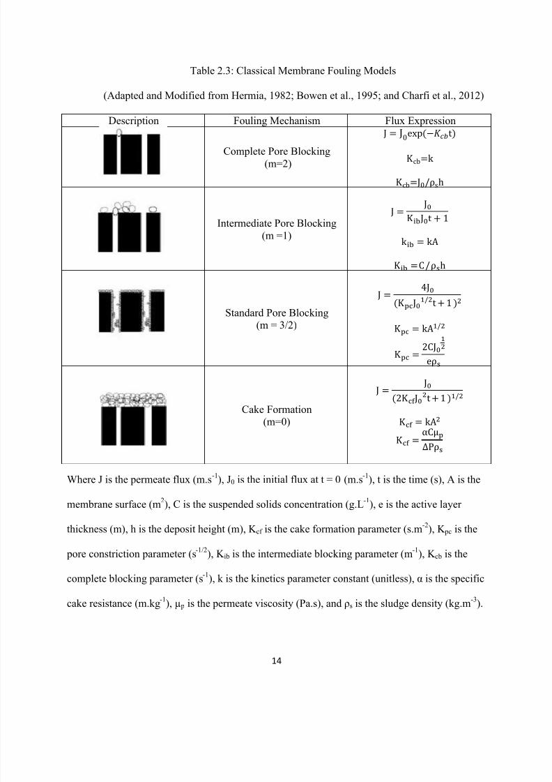
2.6.2. Conceptual Model of Fouling Mechanisms
Conceptual models of fouling mechanisms can be used to identify fouling mechanisms
and to predict the flux decline over time. There are four classical mechanisms that can be used to
define fouling, which are summarized in Table 2.3 (Hwang and Lin, 2002 and Jaffrin et al.,
1997).
8/10/2019 Joshi Priyanka
http://slidepdf.com/reader/full/joshi-priyanka 29/166
13
Complete pore blocking, in which particles of a larger diameter than the pore constrict the
pore entrance and increase filtration resistance.
Intermediate pore blocking follows the same approach as complete blocking, but involves
settling of particles on the existing particles blocking the pores.
Standard pore blocking, which assumes that particles accumulate on the pore walls, thus
causing the volume of the pores to decrease.
Cake formation, which involves accumulation of particles on the membrane surface, thus
resulting in a cake layer.
Conceptual models are aimed to accomplish characterization of fouling mechanisms.
Prediction of fouling mechanisms, as a result of these models, can help prevent and analyze flux
decline effectively. The literature presents models that describe these fouling mechanisms
individually and in combination with each other (Hermia, 1982; Field et al., 1995; Bowen et al.,
1995; Ho and Zydney, 2006; and Charfi et al., 2012). Most of these studies have adapted the
models described by Hermia, (1982), which are summarized in Table 2.3. All the expressions in
Table 2.3 are based on a mathematical model (Equation 2.1), which was presented by Hermia,
(1982) and the flux decline expression (Equation 2.2). The constant m depends on the fouling
mechanism involved in the process and can be found in Table 2.3, along with the definitions of
other parameters.
(
)
Eq. 2.1
Eq. 2.2
8/10/2019 Joshi Priyanka
http://slidepdf.com/reader/full/joshi-priyanka 30/166
14
Table 2.3: Classical Membrane Fouling Models
(Adapted and Modified from Hermia, 1982; Bowen et al., 1995; and Charfi et al., 2012)
Description Fouling Mechanism Flux Expression
Complete Pore Blocking
(m=2)
Intermediate Pore Blocking
(m =1)
Standard Pore Blocking(m = 3/2)
Cake Formation(m=0)
Where J is the permeate flux (m.s-1
), J0 is the initial flux at t = 0 (m.s-1
), t is the time (s), A is the
membrane surface (m2), C is the suspended solids concentration (g.L
-1), e is the active layer
thickness (m), h is the deposit height (m), K cf is the cake formation parameter (s.m-2
), K pc is the
pore constriction parameter (s-1/2), K ib is the intermediate blocking parameter (m-1), K cb is the
complete blocking parameter (s-1
), k is the kinetics parameter constant (unitless), α is the specific
cake resistance (m.kg-1
), µ p is the permeate viscosity (Pa.s), and ρs is the sludge density (kg.m-3
).
8/10/2019 Joshi Priyanka
http://slidepdf.com/reader/full/joshi-priyanka 31/166
15
2.6.3. Prevention and Control of Fouling
In order to determine the optimal operational flux of a system and control fouling, a
critical flux test is often performed. The critical flux is defined as the flux below which minimal
fouling takes place. The method of determining critical flux was introduced by Field et al.,
(1995) and this method was employed in this study. A critical flux test involves increasing the
permeate flux in fixed increments for constant time periods and monitoring the TMP at each
flux. A plot of this data reveals a linear relation between the TMP and flux within the sub-critical
flux range and an exponential relation beyond the critical flux range. This exponential increase
between the two parameters indicates rapid accumulation of foulants.
Operating the membrane below the critical flux has been reported to result in minimal
fouling (Jeison and van Lier, 2006a). Fouling could still take place when operating under the
critical flux; however the rate of fouling is lower below the critical flux (Fan et al., 2006). Thus,
AnMBRs should be operated under the critical flux to minimize fouling.
Fouling can also be minimized by incorporating a relaxation period within the permeation
cycle of the membrane. A relaxed mode of operation involves a cyclic interruption of filtration
by releasing the pressure and allowing the accumulated materials on the membrane surface to be
removed by scouring (Dagnew, 2010). Integration of relaxation in the permeating cycle has been
proven to be effective in controlling anaerobic membrane fouling (Jude, 2006). For instance,
Dagnew et al., (2012) compared the performance of a tubular membrane with continuous
constant permeation for 30 minutes at a flux of 30 litres per m2 per hour (LMH) with a
membrane incorporating a 5 minutes permeation followed by a 1 minute of relaxation cycle.
They observed that relaxation extended the operation of the membrane by limiting the maximum
8/10/2019 Joshi Priyanka
http://slidepdf.com/reader/full/joshi-priyanka 32/166
16
TMP to 30 kilopascals (kPa). However, in continuous operation, the TMP increased almost
linearly to about 80 kPa, thus demonstrating increased fouling of the membrane. Therefore, in an
attempt to minimize fouling, the membrane in this study was operated at a relaxed operation
rather than a continuous operation.
A wide range of relaxation and permeation cycles have been used in the past. Pickel,
(2010) achieved a constant flux of 14 LMH and a TMP of 0.079 kPa with no cleaning by
incorporating a 20 minute permeation followed by 5 hours and 40 minutes of relaxation cycle
during a hollow fibre AnMBR filtration of WAS. On the other hand, Hulse et al., (2009)
observed a flux of 4.6-11.8 LMH and a TMP of 1-1.74 kPa with cleaning at the end of operation
by using a 9 minutes permeation and 1 minute relaxation cycle during a flat sheet AnMBR
filtration of potato solid wastewater. The duration of the relaxation period depends on the
characteristics of the stream being treated, operational conditions such as flux, and the cleaning
frequency. For instance, a more concentrated stream and a higher operational flux with no
cleaning employed may require longer durations of relaxation, as seen with Pickel, (2010). A
few studies have achieved successful operation of the membrane by incorporating relaxation
periods as low as 1 minute with 5 minutes of permeation (Dagnew et al., 2012). This study will
investigate the effect of incorporating a relaxation cycle of 2 minutes with 8 minutes of
permeation on the behaviour of a hollow fibre membrane treating WAS.
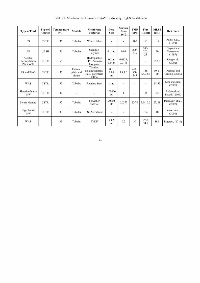
2.6.4. Studies on Membrane Performance of AnMBR Systems Treating High Solids Waste
Table 2.4 summarizes the membrane operating conditions that have been reported in
previous AnMBR studies. From Table 2.4 it can be seen that AnMBRs have been operated over
a broad range of fluxes when treating high solids streams. The range spans from that reported by
8/10/2019 Joshi Priyanka
http://slidepdf.com/reader/full/joshi-priyanka 33/166
17
Saddoud and Sayadi, (2007) (less than 3 LMH) when treating slaughterhouse WW at an MLSS
concentration less than 10 g/L to that of Pierkiel and Lanting, (2005) (146 and 66.7-83 LMH)
when treating a combination of PS and WAS with an MLSS of 5 and 20 g/L. The relatively low
flux reported by Saddoud and Sayadi, (2007) was accomplished with one cleaning cycle after 81
days of operation while Pierkiel and Lanting, (2005) performed daily and monthly cleaning
cycles to maintain higher fluxes.
Although Saddoud and Sayadi, (2007) operated the AnMBR at a lower MLSS than
Pierkiel and Lanting, (2005), they observed a flux decline from 20 to < 3 LMH after start-up.
The low flux observed by Saddoud and Sayadi, (2007) was attributed to pore plugging and cake
formation during filtration, which could have been prevented or controlled by performing regular
maintenance cleaning. Thus, in order to maintain membrane performance, maintenance cleaning
of the membrane may have to be performed in a timely fashion.
High MLSS concentrations do not necessarily translate to a need for frequent cleaning.
For instance, Padmasiri et al., (2007) operated a side stream AnMBR with MLSS concentrations
of 27 and 49 g/L to treat swine manure with no cleaning employed during its operation. The long
term performance of the membrane was attributed to the use of high cross-flow velocities that
prevented deposition of foulants on or in the membrane. However, they also reported a decline in
the biological activity of the micro-organisms due to the high velocities (Section 2.4).
It has been proposed that extremely high shear rates may result in irreversible fouling of
the membrane. If the cross flow velocity or gas sparging rate is too high, this may lead to the
disintegration of biological flocs, thus resulting in finer colloids and extracellular polymeric
substances (EPS) and eventually severe fouling (Chang et al., 2002). Thus, a balance must be
8/10/2019 Joshi Priyanka
http://slidepdf.com/reader/full/joshi-priyanka 34/166
18
maintained between the shear velocity, membrane filtration, frequency of cleaning, and the
biological performance of the reactor.
It has been reported that biomass concentration can significantly affect membrane
performance. As it can be seen from Table 2.4, previous AnMBR studies have been conducted at
MLSS concentrations ranging from 1.8 to 55 g/L (Pillay et al., 1994 and Kim and Jung, 2007).
Jeison and van Lier, (2006b) studied the effect of biomass concentration on the critical flux in a
mesophilic AnMBR, and concluded that an increase in biomass concentration from 20 to 40 g/L
led to a decrease in critical flux from 21 to 9 LMH. Zhang et al., (2007) also reported a similar
observation. Hence, an increase in MLSS concentration reduces the flux range below which
minimal fouling occurs. These reductions in flux are most likely due to the formation of a cake
layer on the membrane surface, thus fouling the membrane and decreasing the resistance of the
membrane.
The impact of membrane type and material of construction on flux has been the subject
of previous studies. Ghyoot and Verstraete, (1997) compared the operation of a ceramic
microfiltration (MF) membrane with a polymer ultrafiltration (UF) membrane for PS treatment
and reported that the ceramic membrane maintained an operational flux of 200-250 LMH and a
TMP of 200 kPa while the flux and TMP for the polymer membrane was 25 LMH and 375 kPa,
respectively. In other words, the polymeric membrane displayed higher resistance to filter a
suspension with similar solids concentration than a ceramic membrane. Although inorganic
membranes such as those made of ceramics offer greater chemical, thermal and hydraulic
resistances, they are not usually preferred as they are not very cost effective (Judd et al., 2004).
For instance, Ghyoot and Verstraete, (1997) estimated the cost of the ceramic MF membrane to
8/10/2019 Joshi Priyanka
http://slidepdf.com/reader/full/joshi-priyanka 35/166
19
be almost twice the cost of the polymer UF membrane. In order to minimize costs, this study
made use of an AnMBR with a polymeric membrane to accomplish permeate filtration.
Operation of membranes at higher fluxes has been reported to cause more fouling of
membranes when compared to lower fluxes. For instance, Lew et al., (2008) investigated the
relationship between flux and the fouling rate of a hollow fibre, MF membrane in an AnMBR. In
this study, fouling rate was defined as an increase in TMP over time. It was found that an
increase in the flux from 3.75 to 11.25 LMH resulted in an increase of the fouling rate from 0.99
to 2.56%.This may be explained by the increase in the rate of mass transfer of sludge particles
towards the membrane surface due to an increase in flux, which led to an increased fouling rate.
Operating temperature has also been found to influence the flux and fouling rate of a
membrane. Membranes have been operated under thermophilic as well as mesophilic conditions
(Kang et al., 2002). Increasing the temperature has been reported to result in a reduced sludge
viscosity which in turn, may increase the operating flux and improve the filtration performance
of the membrane (Dereli et al., 2012). Jeison and van Lier (2006b) observed a higher critical flux
range of 16-23 LMH in a thermophilic AnMBR treating sludge when compared to a mesophilic
reactor, which had a critical flux range of 5-21 LMH. However, long term operation of the
thermophilic reactor resulted in a decreased flux of 2-3 times that of the mesophilic AnMBR and
irreversible fouling. As mentioned earlier, an increase in temperature can lead to an increase in
microbial activity, thus resulting in increased EPS concentrations and smaller flocs. Finer sludge
particles such as colloids may result in the formation of a compact and denser cake, which
decreases the reversibility of flux loss in membranes, thus resulting in irreversible fouling (Jeison
and van Lier, 2007).
8/10/2019 Joshi Priyanka
http://slidepdf.com/reader/full/joshi-priyanka 36/166
20
In summary, the literature reveals that AnMBRs can be operated over a broad range of
conditions; however the flux that can be maintained is a function of sludge characteristics, shear
rate, and cleaning frequency. On the basis of the reviewed literature, the test apparatus employed
in this study was designed to operate with a hollow fiber membrane, an MLSS concentration of
20-25 g/L, a cleaning frequency of 3 times a week, gas sparging to generate shear, a relaxed
mode of operation, and an operating flux that was below the critical flux. This design was
developed to minimize the likelihood of excessive fouling in the experiments.
8/10/2019 Joshi Priyanka
http://slidepdf.com/reader/full/joshi-priyanka 37/166
21
Type of FeedType of
Reactor
Temperature
(°C)Module
Membrane
Material
Pore
Size
SurfaceArea
(m2)
TMP
(kPa)
Flux
(LMH)
MLSS
(g/L)Reference
PS CSTR 35 Tubular Woven Fibre - - 200 50 1.8Pillay et al.,
(1994)
PS UASB 35 Tubular Ceramic,Polymer
0.1 µm 0.05 200,375
200-205,25
50 Ghyoot andVerstraete,(1997)
AlcoholFermentation
Plant WW
CSTR 55 -HydrophobicPPE, Zirconia
Inorganic
0.2m,0.14 m
0.0129,0.0113
- - 2-2.5Kang et al.,
(2002)
PS and WAS CSTR 35Tubular,
plate and
frame
Titanium
dioxide/stainlesssteel, polymeric
teflon
0.1,0.05
µm
1.4,1.6480-550,
345
146,66.7-83
10, 5-20
Pierkiel andLanting, (2005)
WAS CSTR 35 Tubular Stainless Steel 1 µm - - - 18-55Kim and Jung,
(2007)
SlaughterhouseWW
CSTR 37 - -100000
Da1 - <3 <10
Saddoud andSayadi, (2007)
Swine Manure CSTR 37 TubularPolyetherSulfone
20000Da
0.0377 20-70 5.0-10.0 27, 49Padmasiri et al.,
(2007)
High SolidsWW
CSTR 30 Tubular PSF Membrane - - - < 4 40Jeison et al.,
(2008)
WAS - 35 Tubular PVDF0.02µm
0.2 3029.2-34.5
19.8 Dagnew, (2010)
Table 2.4: Membrane Performance of AnMBRs treating High Solids Streams
8/10/2019 Joshi Priyanka
http://slidepdf.com/reader/full/joshi-priyanka 38/166
8/10/2019 Joshi Priyanka
http://slidepdf.com/reader/full/joshi-priyanka 39/166
23
increase in biogas production with respect to the control, while thermal PT at 80°C for one hour
resulted in a 3.5% increase in biogas production compared to the control. In addition, Wang et
al., (1995) showed that the order of pre-treatment efficiency in terms of improvement in methane
generation after pre-treatment was ultrasonic lysis followed by thermal pre-treatment by
autoclave followed by thermal pre-treatment by hot water, and lastly freezing. Therefore
sonication has proved to be more effective in improving the characteristics of WAS than thermal
or peroxide PT.
2.8. Ultrasonic Pre-treatment:
The term ultrasound refers to a sound wave propagating at a frequency higher than the
audible hearing range of human beings (>20 kHz) (Kianmehr, 2010). When an ultrasound wave
travels through a media such as water, it generates numerous cavitation bubbles in the water
(Suslick 1988). Continuous oscillation of the wave causes the local pressure to drop below the
evaporating pressure, which in turn causes these microscopic bubbles to explode (Wandzel et al.,
2011). This abrupt and intense collapse of such a large number of bubbles produces strong
mechanical shear forces that can disintegrate bacterial cells, cells walls, and membranes (Khanal
et al., 2007). The disruption of bacterial cells results in the release of intracellular organic
substances and solubilisation of particulate organic matter (Takatani et al., 1981). It has been
hypothesized that fragmentation of organics due to sonication aids the rate-limiting hydrolysis
reaction in anaerobic digestion and hence can in turn be reflected by increased methane
generation and reduced sludge volume (Show et al., 2007).
Sonication has been reported to be a promising and effective pre-treatment method for
sludge and has been widely researched in laboratory, pilot and recently even in full scale (Tiehm
et al., 1997; Chu et al., 2001; Onyeche et al., 2002; Grönroos et al., 2004; Foladori et al., 2006;
8/10/2019 Joshi Priyanka
http://slidepdf.com/reader/full/joshi-priyanka 40/166
24
Bougrier et al., 2006; Nickel and Neis, 2007; Pham et al., 2007; Zhang et al., 2007, Zhang et al.,
2008; Salsabil et al., 2009; Yan et al., 2010; Kim et al., 2010; Braguglia et al., 2011; and Yaqci
et al., 2011). Table 2.5 provides a summary of some literature involving sonication including
sonication characteristics, solubilisation extent, solids reduction, and biodegradability of WAS,
all factors that are important to this study.
Most of the existing literature assessed the effect of sonication on WAS by monitoring
the soluble chemical oxygen demand (SCOD) release or solubilisation ratio. The solubilisation
ratio is defined as the fraction of total chemical oxygen demand (COD) that is soluble. Past
research has demonstrated that a linear relationship exists between sonication duration and
solubilisation ratio or SCOD concentration. For instance, Chu et al., (2001) concluded that as the
treatment time was increased from 20 to 120 minutes, the fraction of SCOD/TCOD increased
from 3 to 20%. In another study, Kim et al., (2010) observed an increased solubilisation from 8
to 50%, when the the energy supply was increased from 3750 to 45000 kJ/kgTS. Similarly,
Zhang et al., (2007) noticed an SCOD increase of about 3000 mg COD/L after increasing the
sonication duration from 0 to 30 minutes. In another study, Yaqci et al., (2011), reported a 36%
SCOD increase after increasing the sonication duration from 0 to 30 minutes, thus verifying the
linear relationship between sonication duration and SCOD concentration. Thus, most studies
suggest that increasing the sonication duration increases the solubilisation ratio.
Analogous to COD solubilisation, sonication has also been reported to result in increased
solids solubilisation with an increase in sonication duration. For instance, Zhang et al., (2007)
observed a decrease in TSS concentrations of up to 24% when the sonication duration increased
from 0 to 30 minutes, thus demonstrating that sonication solubilizes suspended matter. Salsabil
et al., (2009) also observed a linear relationship between TSS and VSS solubilisation and
8/10/2019 Joshi Priyanka
http://slidepdf.com/reader/full/joshi-priyanka 41/166
25
treatment duration, with a maximum TSS and VSS reduction of 23.3 and 29.7% at a duration of
4 hours. In another study, Bougrier et al., (2006) pre-treated WAS samples of 20 g/L TSS at
specific energies of 6250 kJ/kg TS and 9350 kJ/kg TS. It was found that the VSS/TSS ratio
decreased from 78 to 73% with the energy supplied indicating preferential solubilisation of
organics. Sonication only slightly affected the inert solids, i.e. less than 10% of the inert solids
were solubilized. Thus, sonication significantly affected the organic solids but not the inert
fraction.
Although sonication results in the transfer of materials from the particulate phase into the
soluble phase, no studies discussed in Section 2.5 observed significant reductions in total COD.
In other words, no significant destruction of organic matter took place. Thus, sonication did not
diminish the available resource for methane generation.
In addition to solids and COD solubilisation while conserving TCOD, sonication has also
led to improvements in the biodegradability of WAS. The extent of solubilisation of COD
fractions has been used to assess the impact of pre-treatment on the biodegradability of WAS
(Kianmehr, 2010). For instance, Grönroos et al., 2004 studied the effect of sonication duration on
SCOD increase and methane production from WAS. They noticed that as they increased the
sonication duration from 0 to 10 minutes, the SCOD concentration and methane production
increased from 620 to 4200 mg SCOD/L and from 3.22 to 8.09 m3CH4/kg SCOD consumed in
sample, respectively. In another study, Braguglia et al., (2008) observed that an increase in
SCOD concentration was accompanied by an increase in VSS destruction from 2 to 5% and
biogas volume from 26 to 29% via AD when the sonication duration was increased from 2 to 4
minutes. Similarly, Nickel and Neis, (2007) also observed a biogas volume increase of 16% and
a VSS destruction increase of 40% after increasing the sonication intensity from 5 to 18 W/cm2.
8/10/2019 Joshi Priyanka
http://slidepdf.com/reader/full/joshi-priyanka 42/166
26
Therefore, PT can result in an increase in the extent of destruction by making soluble matter
more readily available to microorganisms.
As previously discussed, sonication of WAS results in the release of material from the
particulate phase to the soluble phase. A considerable fraction of organic materials in WAS
comprises of extra cellular polymeric substances (EPS) (Liu and Fang, 2002). It has been
hypothesized that sonication of WAS results in the solubilisation of EPS, which results in
smaller and finer particles such as colloids (Kianmehr, 2010). Some studies have reported an
increase in colloidal COD (cCOD) with sonication. For this study, cCOD represents the fraction
of COD that can pass through a 1.5 µm filter but not through a 0.45 µm filter. In one study,
Musser, (2010) observed an increase in cCOD/TCOD fraction from 15 to 50% after increasing
the ultrasound dose from 2 to 12 kJ/gTS. Similarly, Kianmehr, (2010) also reported an increase
in cCOD of up to 30% as the sonication duration was increased from 0 to 50 minutes. Kianmehr,
(2010) attributed this increase to the solubilisation of EPS, which resulted in an increase in
cCOD concentration.
In summary, sonication has been found to lead sludge disintegration, reduction in solids
concentration, and increased biodegradability. In addition, it has been reported that sonication
accomplishes all of the above without producing any odours and using any additional chemicals
(Salsabil et al., 2009 and Pilli et al., 2011). Due to all these reasons, sonication is a popular
method of pre-treating WAS. This study will evaluate the effect of sonication on WAS using
existing literature sonication durations to determine if existing results can be replicated.
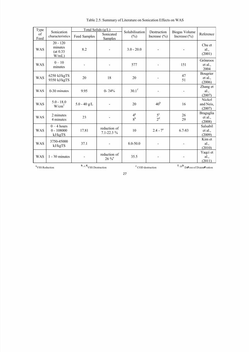
8/10/2019 Joshi Priyanka
http://slidepdf.com/reader/full/joshi-priyanka 43/166
27
Type
ofFeed
Sonicationcharacteristics
Total Solids (g/L)Solubilisation
(%)DestructionIncrease (%)
Biogas VolumeIncrease (%)
ReferenceFeed Samples
SonicatedSamples
WAS
20 - 120
minutes
(at 0.33W/mL)
8.2 - 3.0 - 20.0 - -
Chu et
al.,
(2001)
WAS0 – 10
minutes- - 577 - 151
Grönrooset al.,
2004
WAS6250 kJ/kgTS
9350 kJ/kgTS20 18 20 -
47
51
Bougrieret al.,
(2006)
WAS 0-30 minutes 9.95 0- 24% 30.1f
- -
Zhang et
al.,
(2007)
WAS5.0 - 18.0
W/cm2
5.0 - 40 g/L - 20 40 b
16
Nickel
and Neis,
(2007)
WAS2 minutes
4 minutes23 -
4g
8h
5c
2d
26
29
Bragugliaet al.,
(2008)
WAS0 – 4 hours0 - 108000
kJ/kgTS
17.81reduction of
7.1-22.3 %10 2.4 - 7
e 6.7-83
Salsabilet al.,
(2009)
WAS3750-45000
kJ/kgTS37.1 - 8.0-50.0 - -
Kim et
al.,(2010)
WAS 1 - 30 minutes -reduction of
26 %a 35.5 - -
Yaqci etal.,
(2011)
Table 2.5: Summary of Literature on Sonication Effects on WAS
aVSS Reduction
, c,VSS Destruction
e COD destruction
, g,De ree of Disinte ration
8/10/2019 Joshi Priyanka
http://slidepdf.com/reader/full/joshi-priyanka 44/166
28
2.9. Chemical Pre-treatment
Like sonication, chemical treatment has been reported to break down complex organic
compounds present in WAS and solubilise them. Chemical pre-treatments that have been
evaluated include hydrochloric acid (HCl), sulfuric acid (H2SO4), hydrogen peroxide (H2O2),
Sodium Hydroxide (NaOH), potassium hydroxide (KOH), etc. Out of all of the above, H2O2 is
gaining popularity due to its wide range of treatability. Hydrogen peroxide has been found to be
able to degrade many kinds of organic compounds including those that are moderately and
highly refractory with low biodegradability (Agustina et al., 2005). Moreover it has also been
used to treat inorganics and other compounds such as sulfites, nitrites, hypochlorites, aromatics,
biphenyls, pesticides, herbicides, etc. Thus, H2O2 is capable of degrading a wide variety of
substances.
In the few studies that have been conducted to determine the effect of peroxide dosing on
high solids waste streams it has been concluded that a linear relationship exists between peroxide
dose and solids and COD solubilisation. For instance, Wang et al., (2009) reported that an
increase in the ratio of H2O2/TCOD from 0 to 4.5 (w/w) resulted in an increase in SCOD
concentration by 2000 mg/L. Similarly, they observed a reduction in the VSS/TSS ratio from
0.73 to 0.58 with an increase in the H2O2/TCOD ratio, thus demonstrating solubilisation of
organics. In another study, Eskicioglu et al., (2008) observed an increase in the solubilisation
ratio from 3 to 18% when the peroxide dose increased 0 to 1 g H2O2/g TS of thickened WAS.
Similarly, Dewil et al., (2007) reported an increase in SCOD concentrations from 787 to 2507
mg/L after applying an H2O2 dose range of 5-50 gH2O2/kgDS. Although there has been an
increase in SCOD in these studies, none of them reported an increase in cCOD, thus suggesting
that the effect of H2O2 on cCOD was negligible.
8/10/2019 Joshi Priyanka
http://slidepdf.com/reader/full/joshi-priyanka 45/166
29
A few studies have reported a loss of organic matter due to oxidation by H2O2. For
instance, Eskicioglu et al., (2008) reported losses of 18, 11, 34, and 16% of TCOD, proteins,
sugars, humic acids and total biopolymer concentrations, respectively after treating a 6.4%
thickened WAS samples with 1 g H2O2/gTS. Similarly, Grönroos et al., (2004) observed a 10 %
decrease in COD after treating sludge with 65.8 kgH2O2/tDS. Therefore, treatment with H2O2 in
both cases led to a loss of resource for methane generation.
In addition to solids and COD solubilisation, some studies have observed an increase in
biogas volume when digesting samples after H2O2 dosing. For instance, Song et al., (2012a)
reported that an increase in H2O2 concentration from 3% to 4% improved the biodegradability of
rice straw with a 4.5% TS concentration. The results demonstrated that treatment with 4% H2O2
yielded the highest biogas production, with a biogas volume of 327.5 mL/gVS removed
compared to a control volume of 125 mL/gVS removed. In another study, Song et al., (2012b)
observed an 88% increase in methane yield (compared to the control) by applying a H2O2 dose of
2.68% (w/w TS). Therefore, peroxidation led to the solubilisation of particulates, which resulted
in an improved biodegradability.
In conclusion, pre-treatment of high solids streams with hydrogen peroxide alone has not
been widely researched in literature. However, based on available literature, it can be established
that peroxidation results in COD and solids solubilisation, and thus improved biodegradability.
Peroxidation may also lead to a loss of organic matter, thus diminishing the available resources
for methane generation. Therefore, low concentrations of peroxide addition may be necessary to
avoid loss of biodegradation potential.
8/10/2019 Joshi Priyanka
http://slidepdf.com/reader/full/joshi-priyanka 46/166
30
2.10. Combined Peroxide-Ultrasonic Pre-treatment
Although H2O2 can be used in the treatment of a wide variety of inorganic and organic
pollutants, treatment with H2O2 alone may not be enough to treat high concentrations of some
refractory contaminants (Neyens et al., 2003). Combining H2O2 with other forms of pre-
treatment such as metals like iron, ozone, microwave, and ultrasound has been found to lead to
the generation of strong oxidants in the form of hydroxyl radicals (Eskicioglu et al., 2008).
Hydroxyl radicals are known to be a stronger oxidant than H2O2 itself (Shen and Anastasio,
2012). This combination of pre-treatments known as an advanced oxidation treatment (AOT)
may prove to be more efficient in terms of reducing peroxide doses and increasing the extent of
solubilisation and biodegradability as compared to the individual treatments.
The use of a combination of peroxide and ultrasound for pre-treatment of WAS has not
been widely investigated; however a number of studies with peroxide-microwave, peroxide-
thermal, peroxide-ozone, and peroxide-iron treatments have been reported. The application of an
H2O2/US AOP was evaluated by Grönroos et al., (2004). This study compared the increase in
SCOD concentrations in sludges that were subjected to three types of PTs - sonication at a
specific energy of 6300 kJ/kDS, treatment with 26.3 and 65.8 kgH2O2/tDS for 10 minutes
individually, and treatment with a combination of peroxide and US. It was observed that
individual treatment with US led to the greatest SCOD increase of about 1000 mg/L. Individual
chemical PTs with 26.3 kgH2O2/tDS resulted in an insignificant SCOD increase of 150-200
mg/L, whereas treatment with 65.8 kgH2O2/tDS resulted in a decrease in SCOD. Each AOP
resulted in a higher SCOD concentration than individual chemical treatments but they were still
lower than the US treatment by 11%. This was attributed to the extremely high peroxide doses,
8/10/2019 Joshi Priyanka
http://slidepdf.com/reader/full/joshi-priyanka 47/166
31
which led to a loss of organic matter in the sludge, and thus an insignificant or undesirable
change in SCOD concentrations.
Although the results from Grönroos et al., (2004) indicated that US PT resulted in
improved COD solubilisation as compared to a combined AOP, other AOPs with H2O2 have
shown conflicting results. For instance, Eskicioglu et al., (2008) compared the effects of
microwave, chemical and combined microwave -chemical treatment on solubilisation and
demonstrated that a 25% solubilisation was attained with a combined AOP with a 1 gH2O2/gTS
dose and 120°C temperature. The SCOD/TCOD ratio obtained with individual peroxide and
microwave PT were 14 and 18%, respectively. In another study, Yin et al., (2007) compared the
use of H2O2, ozone, MW, H2O2-ozone, MW-H2O2, MW-ozone, or MW-H2O2-ozone for
solubilisation of sewage sludge. They subjected 90 mL of sludge to a MW temperature of
100°C, peroxide dose of 3 mL, and an ozonation duration of 20 minutes. It was concluded that
the MW-H2O2-ozone combination yielded the greatest COD solubilisation of 37%. Compared to
Grönroos et al., (2004), these AOPs resulted in higher solubilisations than individual PTs. This
may have been due to the significantly lower H2O2 doses as opposed to the ones used by
Grönroos et al., (2004).
As with the other pre-treatments discussed in this chapter, an increase in SCOD due to an
AOP has been reported to result in an improvement in destruction in subsequent anaerobic
digestion. Rivero et al., (2012) observed that thermal PT at 90°C did not lead to any increase in
solids destruction and peroxide PT at 2 gH2O2/gVSS resulted in a maximum VSS destruction
increase of 15.2% via AD. However, a combined AOP resulted in an increase in VSS destruction
of 29%. Thus, the combined AOP was more effective in improving the biodegradability of the
WAS.
8/10/2019 Joshi Priyanka
http://slidepdf.com/reader/full/joshi-priyanka 48/166
32
In conclusion, relatively little research has been done on evaluating the effect of an
H2O2/US AOP on WAS. However some research has been performed with peroxide-microwave,
peroxide-thermal, and peroxide-ozone AOPs. The dose of H2O2 is a significant factor in an AOP
since high doses may lead to loss of organic matter, and thus reduced biodegradability. Using
low peroxide doses in combination with other PTs may result in an increased solubilisation and
biodegradability than individual treatments.
2.11. Integration of Pre-treatment and AnMBRs
As mentioned in Section 2.4, incorporating a membrane into an anaerobic digester can
result in an improved biodegradability compared to conventional AD. However, the
improvement in biodegradability may be limited due to the reactors inability to completely break
down organics and a lengthy and time-consuming digestion process. Moreover, a drawback to
using an AnMBR is membrane fouling, which can be challenging when treating high solids
waste streams such as WAS (Section 2.5). In addition to the high solids concentrations of the
feed, a high SRT/HRT ratio will result in a higher MLSS concentration in the reactor. This may
lead to an increase in membrane fouling and thus high costs associated with cleaning and
replacement of the membrane.
Integration of PT with AnMBRs may provide a solution to increasing the ultimate
biodegradability of WAS. As discussed in section 2.9, it is expected that an AOP using
sonication and hydrogen peroxide will result in solubilisation of particulates thus resulting in an
increased concentration of SCOD. With a significant amount of particulates broken down, a high
sludge age that can be achieved through the use of membranes to prevent biomass washout may
result in an enhanced destruction of compounds. Some studies have been performed to determine
8/10/2019 Joshi Priyanka
http://slidepdf.com/reader/full/joshi-priyanka 49/166
33
the effect of coupling pre-treatment of WAS with AnMBRs. Pickel, (2010) studied the effect of
combining microwave PT of 2% WAS at 67.5 °C with AnMBRs and concluded that this
combination resulted in greater COD degradation of 48.2% than a PT + AD (32.8%) or no PT-
AD/AnMBR (32.2 and 44.4%, respectively) combination. The higher destruction of this
combination indicated that the pre-treatment, presence of the membrane unit, and the decoupling
of the HRT and SRT improved the biodegradation potential of WAS.
Enhanced biodegradability as a result of this combination is expected to result in
decreased fouling of the membrane. As mentioned in section 2.6, pre-treatment of WAS is
expected to reduce the solids concentration of the WAS. This is a benefit not only because it
contributes to high solids reduction but also decreases the solids loading on the membrane in
AnMBRs. Decreased loadings may result in reduced membrane fouling. In addition, decreased
solids concentrations may also lead to cost savings due to reduced shear rates and reduced
requirements for cleaning agents. The literature has established successful operation of
membranes with a PT-AnMBR combination. For instance, Pickel, (2010) achieved high
destruction rates without any maintenance cleaning or replacement of the membrane, thus
demonstrating successful operation of the AnMBR without any major fouling.
As discussed earlier, with pre-treatment, the fraction of colloidal and soluble organic and
inorganic materials in WAS is expected to increase. Hence with an increase in the SRT to HRT
ratio and a membrane, accumulation of the non-and slowly biodegradable particulates may
occur. Therefore it may be possible that an AnMBR treating pre-treated WAS high in cCOD
fractions, long SRTs would cause an additional increase in colloidal fractions in the reactor and
hence membrane performance would decline. In addition, non-biodegradable and inert fractions
may also accumulate in the reactor due to PT and low sludge waste volumes as a result of long
8/10/2019 Joshi Priyanka
http://slidepdf.com/reader/full/joshi-priyanka 50/166
34
sludge ages. However due to the lack of studies determining the impact of PT on fouling, the
above explanations are uncertain and merely an assumption. Therefore, this study will contribute
to filling the void in this area of research, and assess the impact of colloids and other inerts on
membrane performance.
2.12. Summary of Chapter 2
In conclusion, there are a variety of factors affecting the efficiency of a peroxide-sonic
pre-treatment. Most of the studies to date have studies the effect of ultrasound frequency,
ultrasound duration, peroxide dose, and TS of sample on WAS solublization. This study will
build on the previous studies that have assessed the effect of ultrasound duration and hydrogen
peroxide dose on WAS solublization by examining the use of ultrasound durations and peroxide
doses that have been reported in the literature. There have been many studies on the individual
effect of sonication and a few on the effect of peroxide on WAS; however limited information on
the synergistic benefits of peroxide-sonic effect is available. This study aims to determine the
effect of a combined hydrogen peroxide and ultrasound PT system on WAS. A major difference
between existing chemi-sonic treatments and this study is that this study uses a flow through
system to accomplish combined PT of considerably larger volumes of WAS rather than treating
WAS individually with each PT for small volumes.
In addition, this study will couple the PT system with a PVDF submerged hollow fibre
AnMBR to improve biodegradability, a combination which has not been widely reported in
existing literature. In order to determine the effect of PT-AD on WAS biodegradability, a wide
range of physical, chemical and biological parameters such as particle size, TS, VS, SCOD, NH3,
STKN, heterotrophic count and biogas volume has been reported. This study will focus on COD,
8/10/2019 Joshi Priyanka
http://slidepdf.com/reader/full/joshi-priyanka 51/166
35
solids, nitrogen fractions, and membrane performance to assess the process efficiency of PT and
AnMBR. Membrane fouling will be assessed by monitoring TMP when operated at constant flux
and through critical flux tests that will be conducted at steady state.
8/10/2019 Joshi Priyanka
http://slidepdf.com/reader/full/joshi-priyanka 52/166
36
Chapter 3: Pre-treatment of WAS
3.1. Introduction
There are usually two types of waste water sludge that are produced at wastewater
treatment plants (WWTPs) – Primary (PS) and Secondary or Waste Activated Sludge (WAS).
Primary sludge is the product of a mechanical process while WAS is the product of biological
processes such as the activated sludge process. With growing populations the volume of sludge
to be processed at WWTPs is generally increasing. This poses a challenge to plant owners and
operators since the costs associated with sludge treatment/stabilization and disposal may be as
high as 50% of the total cost of treating wastewater (Zhang et al., 2007).
Anaerobic Digestion (AD) is a common sludge stabilization method employed at
WWTPs that not only converts the organic matter into a renewable source of energy i.e. biogas,
but also decreases the amount of solids while destroying a majority of the pathogens in the
sludge (Abelleira et al., 2012). This complex biochemical process employs facultative and
anaerobic microorganisms that work together to achieve stabilization and treatment of sludge in
the absence of oxygen. AD decomposes organic matter in 4 stages: Hydrolysis, Acidogenesis,
Acetogenesis, and Methanogenesis. The performance of anaerobic digestion of WAS is typically
determined by the rate-limiting hydrolysis step since it makes organics available to
microorganisms. This slow process thus requires digesters with long retention times, which
results in an increase in the volume of the digester and associated costs. Numerous studies have
examined methods to increase the rate of hydrolysis and hence reduce the volume needed for
digesters in WWTPs.
Pre-treatment (PT) of sludge has been found to be one way of increasing the rate of
hydrolysis (Shahriari et al., 2011). Pre-treatment leads to the lysis of cells, which in turn causes
8/10/2019 Joshi Priyanka
http://slidepdf.com/reader/full/joshi-priyanka 53/166
37
the release, and thus solubilisation and availability of intracellular matter to microorganisms
(Bougrier et al., 2005). Solubilisation of particulate matter has been found to cause changes in
the physical and chemical properties of a sludge (such as suspended solids and chemical oxygen
demand), thus making it more readily available for microbial growth and metabolic activities
(Pham et al., 2007). Since pre-treatment increases the rate of digestion, this may allow treatment
plants to reduce the retention time in digesters thereby making operation more economically
favourable (Bougrier et al., 2005). A variety of pre-treatments have been proposed for use prior
to anaerobic digestion – mechanical such as sonication, chemical such as peroxidation, and
thermal treatments. The following provide discussion provides a brief description of all three
PTs.
Sonication has been reported to be a promising and effective pre-treatment method to
enhance the biodegradability of sludge and has been widely examined at laboratory, pilot and
recently at full scale (Tiehm et al., 1997; Chu et al., 2001; Onyeche et al., 2002; Grönroos et al.,
2004; Odegaard, 2004; Foladori et al., 2006; Pham et al., 2007; Zhang et al., 2008; Salsabil et al.,
2009; Yan et al., 2010; and Braguglia et al., 2011). When an ultrasound (US) wave travels
through a media such as water, it generates numerous cavitation bubbles in the water (Suslick
1988). Continuous oscillation of the wave causes the local pressure to drop below the
evaporating pressure, which in turn causes these microscopic bubbles to explode (Wandzel et al.,
2011). This abrupt and intense collapse of a large number of bubbles produces strong mechanical
shear forces that can disintegrate bacterial cells, cells walls, and membranes (Khanal et al.,
2007). The disruption of bacterial cells results in the release of intracellular organic substances
and solubilisation of particulate organic matter (Takatani et al., 1981). It has been hypothesized
that fragmentation of organics due to sonication aids the rate-limiting hydrolysis reaction in

8/10/2019 Joshi Priyanka
http://slidepdf.com/reader/full/joshi-priyanka 54/166
38
anaerobic digestion and hence can in turn be reflected by increased methane generation and
reduced sludge volume (Show et al., 2007).
Most reports in the literature describe the effect of sonication on WAS through soluble
chemical oxygen demand (SCOD) release or the solubilisation ratio. The solubilisation ratio is
defined as the fraction of total chemical oxygen demand (COD) that is soluble. Previous studies
have demonstrated a linear relationship between sonication duration and the solubilisation ratio
or SCOD concentration. For instance, Chu et al., (2001) concluded that as the treatment time was
increased from 20 to 120 minutes, the fraction of SCOD/TCOD increased from 3 to 20%.
Similarly, Yaqci et al., (2011), reported a 36% SCOD increase after increasing the sonication
duration from 0 to 30 minutes, thus verifying the linear relationship between sonication duration
and SCOD concentration.
Most studies have also demonstrated that an increase in SCOD concentration is an
indicative of improvement in biodegradability of WAS. For instance, Pham et al., (2007)
observed that sonication of 23 g/L WAS for 60 minutes yielded the highest solubilisation ratio of
79% out of a test range of 20-60 minutes. This increase in SCOD/TCOD corresponded to an
increase in solids destruction of 36.5% in aerobic digestion (Pham et al., 2007). In another study,
Braguglia et al., (2008) observed a 3% increase in biogas volume after increasing the sonication
duration from 2 to 4 minutes. Overall, sonication as a method of PT has been drawing a lot of
attention recently since it can lead to improvements in sludge disintegration and
biodegradability, without producing odours, and using chemicals (Salsabil et al., 2009 and Pilli
et al., 2011).
Thermal hydrolysis is another widely used technique which has been known to increase
the solubilisation ratio, and thus increase destruction rates and biogas volumes (Kepp et al.,
8/10/2019 Joshi Priyanka
http://slidepdf.com/reader/full/joshi-priyanka 55/166
39
2000). Prior studies on thermal pre-treatment of WAS have examined operation over a broad
temperature range of 60 to 270ºC. Thermal PT at temperatures greater than 140ºC has been
reported to be more effective than low temperature thermal PT since higher temperatures are
more effective in breaking down cells (Gureiff et al., 2011). However, treatment above 180ºC
has been discouraged due to the formation of non-biodegradable compounds at high
temperatures (Donoso-Bravo et al., 2011).
It has been found that treatment duration has less effect on sludge characteristics, when
the treatment temperature is between 140 and 180°C (Bougrier et al., 2007; Climent et al., 2007;
and Donoso-Bravo et al., 2011). Most high temperature pre-treatments use a duration of 30-60
minutes (Burger, 2012). A number of studies have been conducted between 150 and 170ºC with
a treatment duration of 30-60 minutes which have proven to improve the solubilisation and
biodegradability or rate of digestion of WAS (Li and Noike., 1992; Bourgrier et al., 2006;
Bougrier et al. 2008; Chauzy et al., 2007; Fdz-Polanco et al., 2008; Ramirez el al., 2009; and
Burger, 2012). For instance, Burger, (2012) pre-treated WAS at 150°C for 30 minutes and
observed a 56% SCOD increase and an increase in the rate of aerobic digestion. In another study,
Li and Noike, (1992) subjected WAS to a heat treatment over a temperature range of 62 – 175°C
and a duration of 15-120 minutes. They concluded that pre-treatment of WAS at 170°C for 60
minutes resulted in the greatest solubilisation and gas production which was 2 times higher than
the control in anaerobic digestion. Similarly, Chauzy et al., (2007) observed an increase in solids
destruction from 25 to 45 % via AD with respect to a control, after pre-treating WAS at 160 °C
for 30 minutes. Therefore, similar to sonication, thermal pre-treatment has been found to result in
an increase and improvement in solubilisation and biodegradation or rate of digestion.
8/10/2019 Joshi Priyanka
http://slidepdf.com/reader/full/joshi-priyanka 56/166
40
Like sonication and thermal PTs, chemical treatment can also break down complex
organic compounds present in WAS, solubilise them and improve WAS biodegradability.
Chemical pre-treatments that have been evaluated include hydrochloric acid (HCl), sulfuric acid
(H2SO4), hydrogen peroxide (H2O2), sodium hydroxide (NaOH), potassium hydroxide (KOH),
etc. Out of these, H2O2 is gaining popularity due to its wide range of treatability. Hydrogen
peroxide has been found to be able to degrade many kinds of organic compounds including those
that are moderately and highly refractory with low biodegradability (Agustina et al., 2005).
Moreover it has also been used to treat inorganics and other compounds such as sulfites, nitrites,
hypochlorites, aromatics, biphenyls, pesticides, herbicides, etc. Thus, H2O2 is capable of
degrading a wide variety of substances.
Literature has shown that a linear relationship exists between peroxide dose and SCOD
concentrations and biodegradability of WAS. For instance, Eskicioglu et al., (2008) observed an
increase in the solubilisation ratio from 3 to 18% after applying a peroxide dose range of 0 to 1
gH2O2/gTS to thickened WAS samples. Similarly, Dewil et al., (2007) reported an increase in
SCOD release from 787 to 2507 mg/L after applying an H2O2 dose range of 5-50 gH2O2/kgDS.
Song et al., (2012) reported that an increase in H2O2 concentration from 3% to 4% improved the
solubilisation and biodegradability of rice straw with 4.5% TS concentration. The results
demonstrated that treatment with 4% H2O2 yielded the highest biogas production, with a biogas
volume of 327.5 mL/gVS removed compared to a control volume of 125 mL/gVS removed.
Although H2O2 can be used in the treatment of a wide variety of inorganic and organic
pollutants, treatment with H2O2 alone may not be feasible for treating high concentrations of
some refractory contaminants (Neyens et al., 2003). Combining H2O2 with other forms of pre-
treatment such as metals like iron, ozone, microwave, and ultrasound has been found to lead to
8/10/2019 Joshi Priyanka
http://slidepdf.com/reader/full/joshi-priyanka 57/166
41
the generation of strong oxidants in the form of hydroxyl radicals (Eskicioglu et al., 2008).
Hydroxyl radicals are known to be stronger oxidants than H2O2 itself (Shen and Anastasio,
2012). This combination of pre-treatments known as an advanced oxidation process (AOP) may
prove to be more efficient in terms of reducing peroxide doses and increasing the extent of
solubilisation and biodegradability as compared to the individual treatments.
The use of a combination of peroxide and ultrasound for pre-treatment of WAS has not
been widely researched; however a number of studies of peroxide-microwave, peroxide-thermal,
peroxide-ozone, and peroxide-iron treatments have been reported. Grönroos et al., (2004)
compared the increase in SCOD concentrations among sludge samples that were sonicated at a
specific energy of 6300 kJ/kgDS, treated with 26.3 and 65.8 kgH2O2/tDS for 10 minutes
individually, and subjected to a combination of both peroxide doses and US. It was observed that
individual treatment with US led to the greatest SCOD increase of about 1000 mg/L. Individual
chemical PTs with 26.3 kgH2O2/tDS resulted in an insignificant SCOD increase of 150-200
mg/L, whereas treatment with 65.8 kgH2O2/tDS resulted in a decrease in SCOD. Each AOP
resulted in a higher SCOD concentration than the individual chemical treatments but they were
still lower than the US treatment by 11%. This was attributed to the high peroxide doses, which
led to a loss of organic matter in the sludge, and thus an insignificant or undesirable change in
SCOD concentrations.
Although the results from Grönroos et al., (2004) indicated that US PT resulted in greater
COD solubilisation than the combined AOP, other AOPs with H2O2 have shown differing
results. For instance, Eskicioglu et al., (2008) compared microwave, chemical and combined
micro-chemical treatment and found 25% solubilisation was attained with a combined AOP with
a 1 gH2O2/gTS dose and 120°C temperature. The SCOD/TCOD ratios obtained with individual
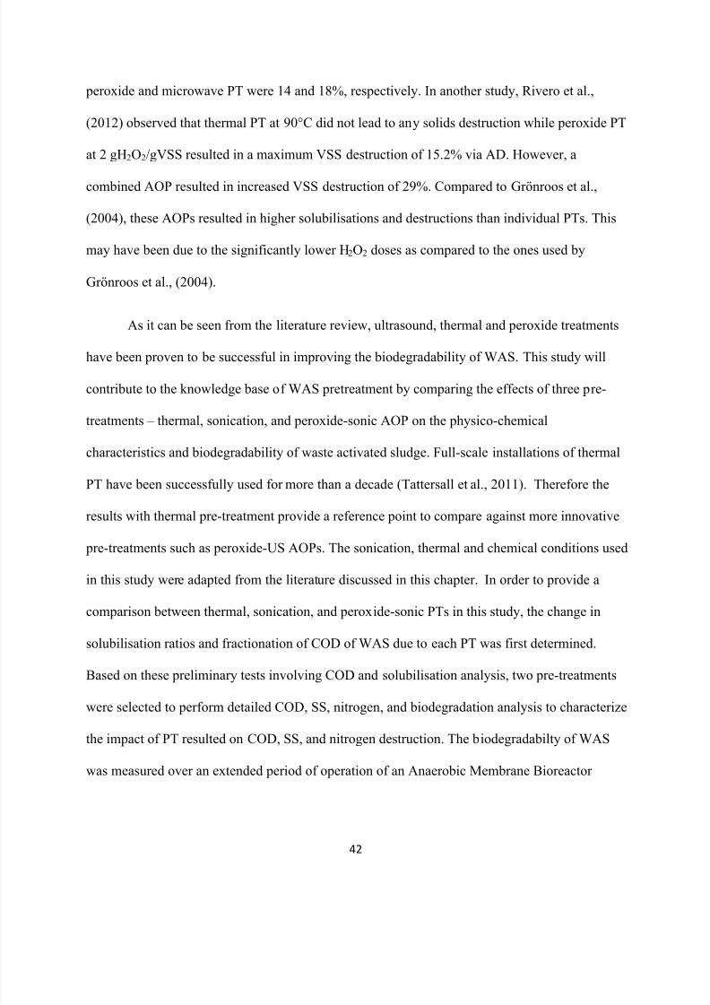
8/10/2019 Joshi Priyanka
http://slidepdf.com/reader/full/joshi-priyanka 58/166
42
peroxide and microwave PT were 14 and 18%, respectively. In another study, Rivero et al.,
(2012) observed that thermal PT at 90°C did not lead to any solids destruction while peroxide PT
at 2 gH2O2/gVSS resulted in a maximum VSS destruction of 15.2% via AD. However, a
combined AOP resulted in increased VSS destruction of 29%. Compared to Grönroos et al.,
(2004), these AOPs resulted in higher solubilisations and destructions than individual PTs. This
may have been due to the significantly lower H2O2 doses as compared to the ones used by
Grönroos et al., (2004).
As it can be seen from the literature review, ultrasound, thermal and peroxide treatments
have been proven to be successful in improving the biodegradability of WAS. This study will
contribute to the knowledge base of WAS pretreatment by comparing the effects of three pre-
treatments – thermal, sonication, and peroxide-sonic AOP on the physico-chemical
characteristics and biodegradability of waste activated sludge. Full-scale installations of thermal
PT have been successfully used for more than a decade (Tattersall et al., 2011). Therefore the
results with thermal pre-treatment provide a reference point to compare against more innovative
pre-treatments such as peroxide-US AOPs. The sonication, thermal and chemical conditions used
in this study were adapted from the literature discussed in this chapter. In order to provide a
comparison between thermal, sonication, and peroxide-sonic PTs in this study, the change in
solubilisation ratios and fractionation of COD of WAS due to each PT was first determined.
Based on these preliminary tests involving COD and solubilisation analysis, two pre-treatments
were selected to perform detailed COD, SS, nitrogen, and biodegradation analysis to characterize
the impact of PT resulted on COD, SS, and nitrogen destruction. The biodegradabilty of WAS
was measured over an extended period of operation of an Anaerobic Membrane Bioreactor
8/10/2019 Joshi Priyanka
http://slidepdf.com/reader/full/joshi-priyanka 59/166
43
(AnMBR). The methods of sample analysis and the operational conditions for the AnMBR used
in this study are described in Section 3.2.
3.2. Materials and Methods
3.2.1. Waste Activated Sludge Characteristics
Secondary sludge was obtained from the Waterloo WWTP located in Waterloo, ON, Canada,
which has a daily operating capacity of 72.73 ML. This plant makes use of a conventional
wastewater treatment process and consists of preliminary, primary, and secondary treatment. For
this study, secondary sludge samples were concentrated by settling at 4˚C for not more than a
day until a desired concentration of about 7.5 gTSS/L was reached. Table 3.1 presents the
characteristics of the thickened WAS that was employed in this study.
Table 3.1: Characteristics of Thickened WAS
Parameters Concentration
pH 7.49
TS (g/L) 7.06 ± 0.17
Total COD (g/L) 7.55 ± 0.87
Total TKN (gN/L) 0.66 ± 0.05
Soluble COD (g/L) 0.08 ± 0.04
Soluble TKN (gN/L) 0.03 ± 0.01
Ammonia (gN/L) 0.02 ± 0.01
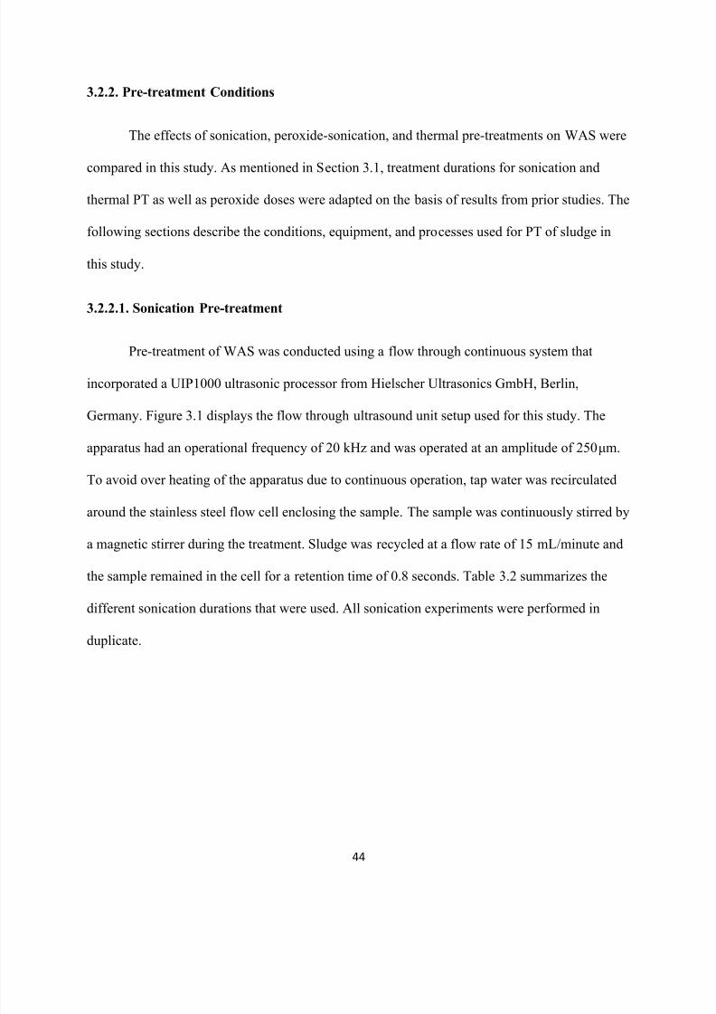
8/10/2019 Joshi Priyanka
http://slidepdf.com/reader/full/joshi-priyanka 60/166
44
3.2.2. Pre-treatment Conditions
The effects of sonication, peroxide-sonication, and thermal pre-treatments on WAS were
compared in this study. As mentioned in Section 3.1, treatment durations for sonication and
thermal PT as well as peroxide doses were adapted on the basis of results from prior studies. The
following sections describe the conditions, equipment, and processes used for PT of sludge in
this study.
3.2.2.1. Sonication Pre-treatment
Pre-treatment of WAS was conducted using a flow through continuous system that
incorporated a UIP1000 ultrasonic processor from Hielscher Ultrasonics GmbH, Berlin,
Germany. Figure 3.1 displays the flow through ultrasound unit setup used for this study. The
apparatus had an operational frequency of 20 kHz and was operated at an amplitude of 250 μm.
To avoid over heating of the apparatus due to continuous operation, tap water was recirculated
around the stainless steel flow cell enclosing the sample. The sample was continuously stirred by
a magnetic stirrer during the treatment. Sludge was recycled at a flow rate of 15 mL/minute and
the sample remained in the cell for a retention time of 0.8 seconds. Table 3.2 summarizes the
different sonication durations that were used. All sonication experiments were performed in
duplicate.
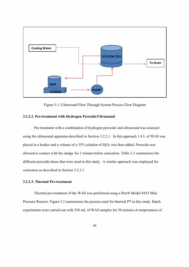
8/10/2019 Joshi Priyanka
http://slidepdf.com/reader/full/joshi-priyanka 61/166
45
Figure 3.1: Ultrasound Flow Through System Process Flow Diagram
3.2.2.2. Pre-treatment with Hydrogen Peroxide/Ultrasound
Pre-treatment with a combination of hydrogen peroxide and ultrasound was assessed
using the ultrasound apparatus described in Section 3.2.2.1. In this approach 1.6 L of WAS was
placed in a beaker and a volume of a 35% solution of H2O2 was then added. Peroxide was
allowed to contact with the sludge for 1 minute before sonication. Table 3.2 summarizes the
different peroxide doses that were used in this study. A similar approach was employed for
sonication as described in Section 3.2.2.1.
3.2.2.3. Thermal Pre-treatment
Thermal pre-treatment of the WAS was performed using a Parr® Model 4563 Mini
Pressure Reactor. Figure 3.2 summarizes the process used for thermal PT in this study. Batch
experiments were carried out with 350 mL of WAS samples for 30 minutes at temperatures of
To Drain
WAS
STIRRERPUMP
US FLOW CELL
Cooling Water
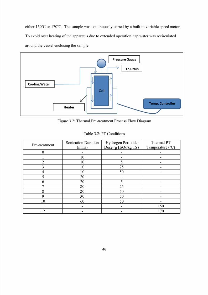
8/10/2019 Joshi Priyanka
http://slidepdf.com/reader/full/joshi-priyanka 62/166
46
either 150ºC or 170ºC. The sample was continuously stirred by a built in variable speed motor.
To avoid over heating of the apparatus due to extended operation, tap water was recirculated
around the vessel enclosing the sample.
Figure 3.2: Thermal Pre-treatment Process Flow Diagram
Table 3.2: PT Conditions
Pre-treatmentSonication Duration
(mins)
Hydrogen Peroxide
Dose (g H2O2/kg TS)
Thermal PT
Temperature (ºC)
0 - - -
1 10 - -
2 10 5 -
3 10 25 -
4 10 50 -
5 20 - -
6 20 5 -
7 20 25 -
8 20 50 -
9 30 50 -
10 60 50 -
11 - - 15012 - - 170
Temp. Controller
To Drain
Cell
Pressure Gauge
Heater
Cooling Water
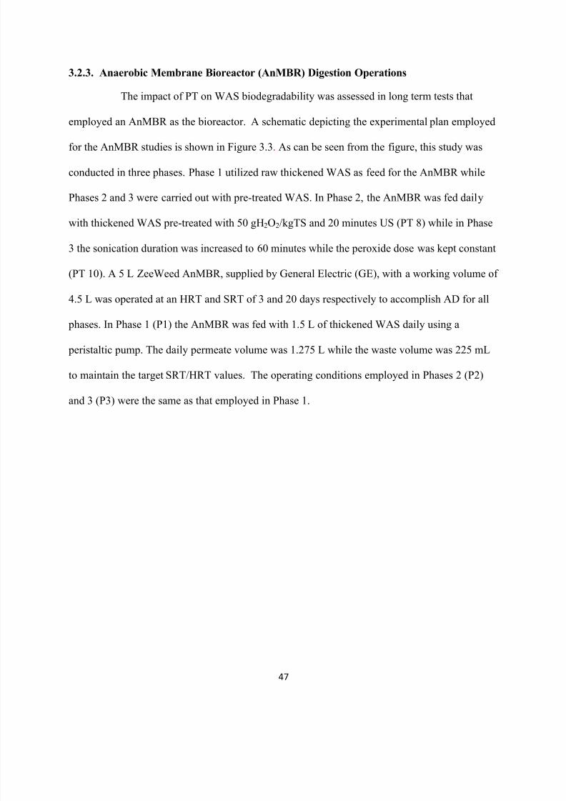
8/10/2019 Joshi Priyanka
http://slidepdf.com/reader/full/joshi-priyanka 63/166
47
3.2.3. Anaerobic Membrane Bioreactor (AnMBR) Digestion Operations
The impact of PT on WAS biodegradability was assessed in long term tests that
employed an AnMBR as the bioreactor. A schematic depicting the experimental plan employed
for the AnMBR studies is shown in Figure 3.3. As can be seen from the figure, this study was
conducted in three phases. Phase 1 utilized raw thickened WAS as feed for the AnMBR while
Phases 2 and 3 were carried out with pre-treated WAS. In Phase 2, the AnMBR was fed daily
with thickened WAS pre-treated with 50 gH2O2/kgTS and 20 minutes US (PT 8) while in Phase
3 the sonication duration was increased to 60 minutes while the peroxide dose was kept constant
(PT 10). A 5 L ZeeWeed AnMBR, supplied by General Electric (GE), with a working volume of
4.5 L was operated at an HRT and SRT of 3 and 20 days respectively to accomplish AD for all
phases. In Phase 1 (P1) the AnMBR was fed with 1.5 L of thickened WAS daily using a
peristaltic pump. The daily permeate volume was 1.275 L while the waste volume was 225 mL
to maintain the target SRT/HRT values. The operating conditions employed in Phases 2 (P2)
and 3 (P3) were the same as that employed in Phase 1.
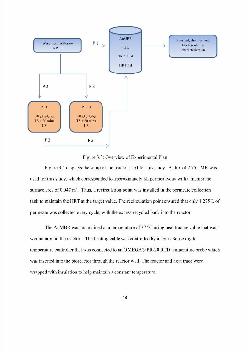
8/10/2019 Joshi Priyanka
http://slidepdf.com/reader/full/joshi-priyanka 64/166
48
Figure 3.3: Overview of Experimental Plan
Figure 3.4 displays the setup of the reactor used for this study. A flux of 2.75 LMH was
used for this study, which corresponded to approximately 3L permeate/day with a membrane
surface area of 0.047 m2. Thus, a recirculation point was installed in the permeate collection
tank to maintain the HRT at the target value. The recirculation point ensured that only 1.275 L of
permeate was collected every cycle, with the excess recycled back into the reactor.
The AnMBR was maintained at a temperature of 37 °C using heat tracing cable that was
wound around the reactor. The heating cable was controlled by a Dyna-Sense digital
temperature controller that was connected to an OMEGA® PR-20 RTD temperature probe which
was inserted into the bioreactor through the reactor wall. The reactor and heat trace were
wrapped with insulation to help maintain a constant temperature.
WAS from Waterloo
WWTP
AnMBR
4.5 L
SRT 20 d
HRT 3 d
Physical, chemical and
biodegradation
characterization
PT 8
50 gH2O2/kg
TS + 20 mins
US
PT 10
50 gH2O2/kg
TS + 60 mins
US
P 1
P 2 P 3
P 2 P 3
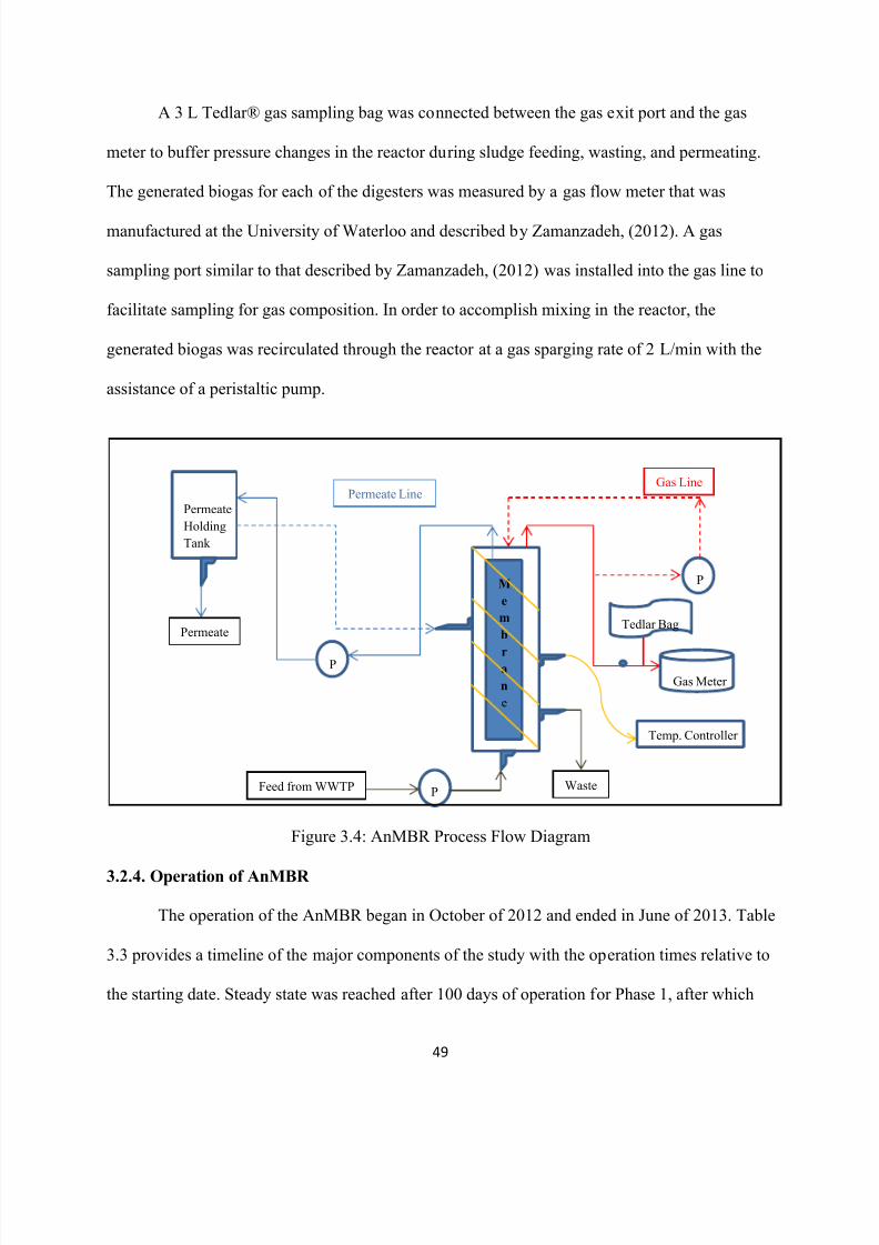
8/10/2019 Joshi Priyanka
http://slidepdf.com/reader/full/joshi-priyanka 65/166
49
A 3 L Tedlar® gas sampling bag was connected between the gas exit port and the gas
meter to buffer pressure changes in the reactor during sludge feeding, wasting, and permeating.
The generated biogas for each of the digesters was measured by a gas flow meter that was
manufactured at the University of Waterloo and described by Zamanzadeh, (2012). A gas
sampling port similar to that described by Zamanzadeh, (2012) was installed into the gas line to
facilitate sampling for gas composition. In order to accomplish mixing in the reactor, the
generated biogas was recirculated through the reactor at a gas sparging rate of 2 L/min with the
assistance of a peristaltic pump.
Figure 3.4: AnMBR Process Flow Diagram
3.2.4.
Operation of AnMBR
The operation of the AnMBR began in October of 2012 and ended in June of 2013. Table
3.3 provides a timeline of the major components of the study with the operation times relative to
the starting date. Steady state was reached after 100 days of operation for Phase 1, after which
M
e
m
b
ra
n
e
Temp. Controller
Tedlar Bag
P
P
PFeed from WWTP Waste
Permeate
Holding
Tank
Gas Meter
Permeate
Gas LinePermeate Line
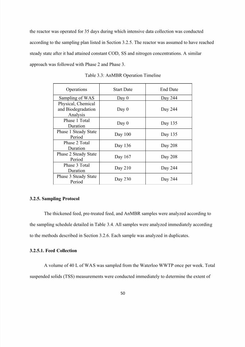
8/10/2019 Joshi Priyanka
http://slidepdf.com/reader/full/joshi-priyanka 66/166
50
the reactor was operated for 35 days during which intensive data collection was conducted
according to the sampling plan listed in Section 3.2.5. The reactor was assumed to have reached
steady state after it had attained constant COD, SS and nitrogen concentrations. A similar
approach was followed with Phase 2 and Phase 3.
Table 3.3: AnMBR Operation Timeline
Operations Start Date End Date
Sampling of WAS Day 0 Day 244
Physical, Chemical
and Biodegradation
Analysis
Day 0 Day 244
Phase 1 TotalDuration
Day 0 Day 135
Phase 1 Steady State
PeriodDay 100 Day 135
Phase 2 Total
DurationDay 136 Day 208
Phase 2 Steady StatePeriod
Day 167 Day 208
Phase 3 TotalDuration
Day 210 Day 244
Phase 3 Steady State
PeriodDay 230 Day 244
3.2.5. Sampling Protocol
The thickened feed, pre-treated feed, and AnMBR samples were analyzed according to
the sampling schedule detailed in Table 3.4. All samples were analyzed immediately according
to the methods described in Section 3.2.6. Each sample was analyzed in duplicates.
3.2.5.1. Feed Collection
A volume of 40 L of WAS was sampled from the Waterloo WWTP once per week. Total
suspended solids (TSS) measurements were conducted immediately to determine the extent of
8/10/2019 Joshi Priyanka
http://slidepdf.com/reader/full/joshi-priyanka 67/166
51
thickening that was required to achieve the desired feed TSS concentration. WAS samples were
then thickened accordingly by settling the WAS samples overnight until a TSS concentration of
7.5 g/L was attained. COD, Total Kjeldahl Nitrogen (TKN), ammonia, and SS measurements
were performed on the thickened feed (F) samples on the following day.
3.2.5.2. PT of WAS
A volume of 1.6 L of thickened feed samples was subjected to pre-treatment daily
according to the protocol in Section 3.2.2. This ensured that fresh PT feed was fed to the reactor
everyday. The pre-treated feed was sampled and analyzed for COD, TKN, ammonia, and SS
once per week.
3.2.5.3. AnMBR Monitoring
The waste (W) and permeate (P) streams from the AnMBR were sampled and analyzed
for COD, TKN, and ammonia twice a week. The waste stream was sampled and analysed for
TSS and VSS once a week. The pH of the waste and permeate was measured daily. The biogas
composition and volatile acids to alkalinity ratio (VFA/ALK) were monitored thrice a week.
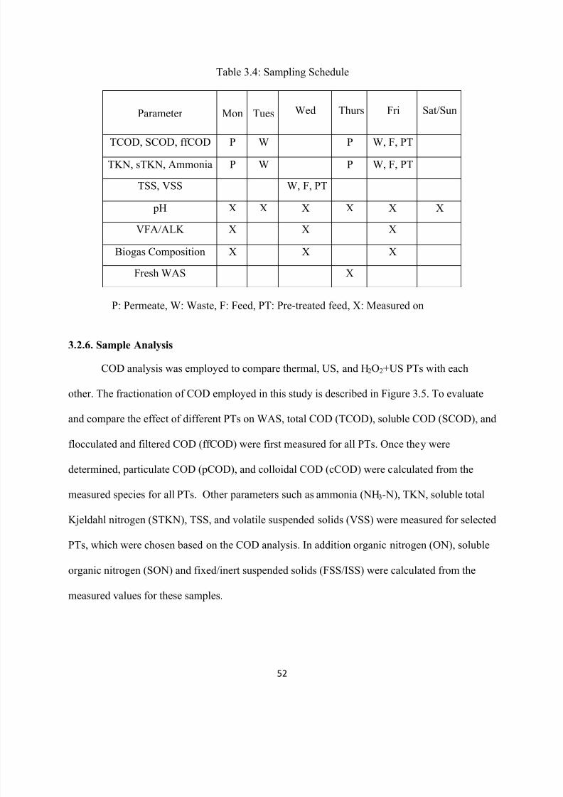
8/10/2019 Joshi Priyanka
http://slidepdf.com/reader/full/joshi-priyanka 68/166
52
Table 3.4: Sampling Schedule
Parameter Mon Tues Wed Thurs Fri Sat/Sun
TCOD, SCOD, ffCOD P W P W, F, PT
TKN, sTKN, Ammonia P W P W, F, PT
TSS, VSS W, F, PT
pH X X X X X X
VFA/ALK X X X
Biogas Composition X X X
Fresh WAS X
3.2.6. Sample Analysis
COD analysis was employed to compare thermal, US, and H2O2+US PTs with each
other. The fractionation of COD employed in this study is described in Figure 3.5. To evaluate
and compare the effect of different PTs on WAS, total COD (TCOD), soluble COD (SCOD), and
flocculated and filtered COD (ffCOD) were first measured for all PTs. Once they were
determined, particulate COD (pCOD), and colloidal COD (cCOD) were calculated from the
measured species for all PTs. Other parameters such as ammonia (NH3-N), TKN, soluble total
Kjeldahl nitrogen (STKN), TSS, and volatile suspended solids (VSS) were measured for selected
PTs, which were chosen based on the COD analysis. In addition organic nitrogen (ON), soluble
organic nitrogen (SON) and fixed/inert suspended solids (FSS/ISS) were calculated from the
measured values for these samples.
P: Permeate, W: Waste, F: Feed, PT: Pre-treated feed, X: Measured on
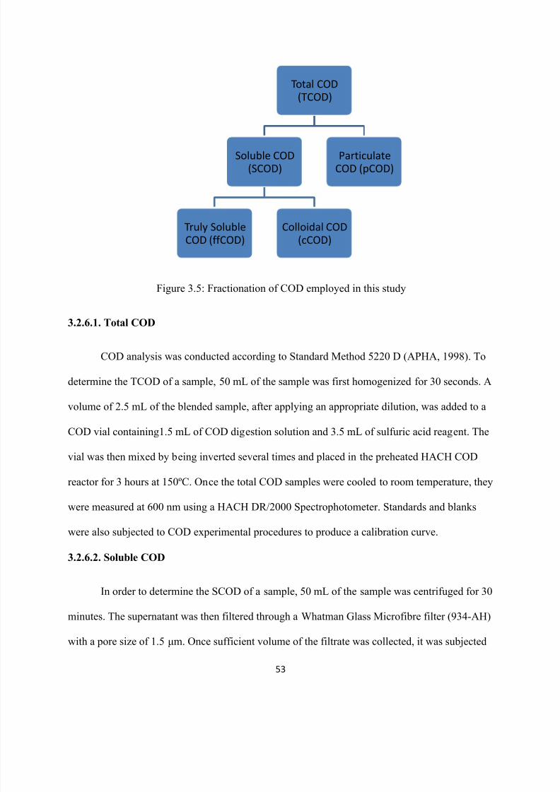
8/10/2019 Joshi Priyanka
http://slidepdf.com/reader/full/joshi-priyanka 69/166
53
Figure 3.5: Fractionation of COD employed in this study
3.2.6.1. Total COD
COD analysis was conducted according to Standard Method 5220 D (APHA, 1998). To
determine the TCOD of a sample, 50 mL of the sample was first homogenized for 30 seconds. A
volume of 2.5 mL of the blended sample, after applying an appropriate dilution, was added to a
COD vial containing1.5 mL of COD digestion solution and 3.5 mL of sulfuric acid reagent. The
vial was then mixed by being inverted several times and placed in the preheated HACH COD
reactor for 3 hours at 150ºC. Once the total COD samples were cooled to room temperature, they
were measured at 600 nm using a HACH DR/2000 Spectrophotometer. Standards and blanks
were also subjected to COD experimental procedures to produce a calibration curve.
3.2.6.2.
Soluble COD
In order to determine the SCOD of a sample, 50 mL of the sample was centrifuged for 30
minutes. The supernatant was then filtered through a Whatman Glass Microfibre filter (934-AH)
with a pore size of 1.5 μm. Once sufficient volume of the filtrate was collected, it was subjected
Total COD(TCOD)
Soluble COD(SCOD)
Truly SolubleCOD (ffCOD)
Colloidal COD(cCOD)
ParticulateCOD (pCOD)
8/10/2019 Joshi Priyanka
http://slidepdf.com/reader/full/joshi-priyanka 70/166
54
to dilution and subsequent measurement as per as the protocol followed with TCOD in Section
3.2.6.1.
3.2.6.3. Flocculated and Filtered COD
The flocculated-filtered COD (ffCOD) was considered to represent the truly soluble COD
(Mamais et al., 1993). A volume of 2.5 mL of 100 mg/L alum stock solution was added to 25 mL
of the sCOD filtrate and mixed vigorously for 30 seconds. This was followed by allowing the
filtrate to settle for 10 minutes, after which it was subjected to 15 minutes of centrifugation. The
supernatant obtained from this process was then filtered using a 0.45 μm pore size filter. Once
sufficient volume of the filtrate was collected, it was subjected to dilution and subsequent
measurement as per as the protocol followed with TCOD in Section 3.2.6.1.
3.2.6.4. Ammonia
The analytical method employed for ammonia was conducted according to Standard
Method 4500 F (APHA, 1998). A Bran and Luebbe AutoAnalyzer 3 was used to colorimetrically
measure the concentration of ammonia in samples. A portion of the sample that was generated
for SCOD analysis was used for this purpose after applying an adequate dilution factor. In the
AutoAnalyzer the ammonia in a sample was reacted with sodium hypochlorite, a sodium
hydroxide buffer solution, and phenol to produced indophenol. Sodium nitroprusside present in
the buffer reagent intensified the colour prior to colorimetric analysis at 660 nm.
3.2.6.5. Total Kjeldahl Nitrogen
A portion of the sample that was generated for TCOD analysis was used for TKN
analysis. The TKN analysis method employed in this study was developed in the Environment
Canada Wastewater Technology Center in Burlington, Ontario. It involved adding 1.5 mL of a
digestion solution to 1 mL of the homogenized sample in a digestion flask. The digestion
8/10/2019 Joshi Priyanka
http://slidepdf.com/reader/full/joshi-priyanka 71/166
55
solution was prepared by first dissolving 40 g potassium sulfate and 2 mL selenium oxychloride
in 250 mL sulfuric acid. This solution was then diluted by the addition of deionized water to
reach a volume of 500 mL. After addition of the digestion solution the sample was digested in a
Bran and Luebbe BD-40 block digester at 220ºC for 1.5 hours followed by digestion at 380ºC for
2.5 hours. This digestion converted all the organic nitrogen to ammonia. The samples were
allowed to cool down to room temperature overnight, diluted, and analysed the next day using
the ammonia analysis described in Section 3.2.6.4.
3.2.6.6. Soluble TKN
A portion of the sample that was generated for measuring SCOD was used for measuring
STKN. The same digestion procedure was followed as described in Section 3.2.6.5. The
ammonia analyzer was used to measure the concentration of STKN.
3.2.6.7. Nitrate
Nitrate measurements were conducted as per HACH Method 8039 (HACH, 1997). A
portion of the sample that was generated for measuring ffCOD was used to measure nitrate. One
pouch of HACH NitraVER® 5 Nitrate Reagent power was added to 25 mL of the sample. The
sample was mixed vigorously using a shaker for 1 minute and allowed to rest for 5 minutes. The
sample was then analyzed at 400 nm using the HACH DR/200 Spectrophotometer.
3.2.6.8. Suspended Solids
The solids analysis in this study was based on Standard Methods 2540 D and E for total
suspended solids and volatile suspended solids, respectively (APHA 1998). Total suspended
solids were measured by filtering 5 mL of a sample through a 1.5 µm pore size filter that had
been previously dried at 550ºC. The filter was then dried at 105ºC for at least one hour. The
increase in mass was then employed to calculate the TSS. The same filter was then combusted at
8/10/2019 Joshi Priyanka
http://slidepdf.com/reader/full/joshi-priyanka 72/166
56
550ºC for at least 45 minutes. The loss of mass due to ignition was then employed to calculate
the VSS. The difference between TSS and VSS employed to estimate the fixed suspended solids
(FSS).
3.2.6.9. Volatile Fatty Acids to Alkalinity Ratio
The VFA/Alk ratio was measured to monitor the stability of the AnMBR. A 4-point
titration method was adapted from Buchauer, (1998) to determine the ratio for this study. A
volume of 50 mL of permeate sample was titrated with 0.1 N sulfuric acid solution with constant
mixing until pHs of 5, 4.3, and 4 were reached. The volume of titrant used to attain each pH end
point was recorded and the alkalinity and VFA concentration were calculated according to the
scheme and formulae provided by Buchauer, (1998).
3.2.6.10. pH
The pH of the permeate and waste samples from the AnMBR was measured daily using
an Omega PHB-600R pH Benchtop Meter.
3.3. Results and Discussion
3.3.1.
Preliminary Pre-treatment Tests
Preliminary tests were conducted to compare the effect of thermal, ultrasonic, and
peroxide-sonic pre-treatments on WAS. The primary response used in determining the preferred
pre-treatment in this preliminary study was the COD solubilisation ratio. As discussed in Section
3.1, the COD solubilisation ratio was defined as the fraction of total COD that was soluble after
PT. Although the SCOD/TCOD ratio was the main parameter of interest for determining the
preferred PT method, other factors such as loss of TCOD and increase in cCOD and ffCOD
fractions were also taken into consideration when making the decision. All preliminary tests
were performed in duplicate with fresh WAS from the Waterloo WWTP.
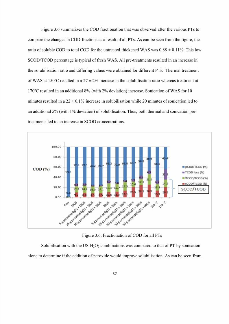
8/10/2019 Joshi Priyanka
http://slidepdf.com/reader/full/joshi-priyanka 73/166
57
Figure 3.6 summarizes the COD fractionation that was observed after the various PTs to
compare the changes in COD fractions as a result of all PTs. As can be seen from the figure, the
ratio of soluble COD to total COD for the untreated thickened WAS was 0.88 ± 0.11%. This low
SCOD/TCOD percentage is typical of fresh WAS. All pre-treatments resulted in an increase in
the solubilisation ratio and differing values were obtained for different PTs. Thermal treatment
of WAS at 150ºC resulted in a 27 ± 2% increase in the solubilisation ratio whereas treatment at
170ºC resulted in an additional 8% (with 2% deviation) increase. Sonication of WAS for 10
minutes resulted in a 22 ± 0.1% increase in solubilisation while 20 minutes of sonication led to
an additional 5% (with 1% deviation) of solubilisation. Thus, both thermal and sonication pre-
treatments led to an increase in SCOD concentrations.
Figure 3.6: Fractionation of COD for all PTs
Solubilisation with the US-H2O2 combinations was compared to that of PT by sonication
alone to determine if the addition of peroxide would improve solubilisation. As can be seen from
8/10/2019 Joshi Priyanka
http://slidepdf.com/reader/full/joshi-priyanka 74/166
58
Figure 3.6, the peroxide-sonic PTs resulted in greater solubilisation than sonication alone. For
instance, sonication at 20 minutes resulted in a solubilisation ratio of 27 ± 1%. However the
maximum solubilisation that was achieved with addition of peroxide to a sample sonicated for 20
minutes at a maximum dosage of 50 gH2O2/kgTS was 32%. By comparison, Grönroos et al.,
(2004) reported that the COD solubilisation ratio due to a peroxide-sonic PT of excess sludge
was 11% lower than the solubilisation ratio due to sonication alone (Section 3.1). This was
attributed to high peroxide doses that were employed in the previous study which led to a loss of
organic matter in the sludge, and thus an insignificant or undesirable change in SCOD
concentrations. Since the peroxide doses used in this study were much lower than those used by
Grönroos et al., (2004), no significant loss of organic matter occurred due to peroxidation
(Figure 3.6). The COD solubilisation results from this study thus followed those reported in other
studies that used low doses of peroxide (Eskicioglu et al., 2008 and Rivero et al., 2012), i.e. a
combined PT resulted in higher solubilisation than individual PT alone.
Treatment with H2O2 in combination with sonication as an AOP was studied with a 2 x 4
factorial design, with two US durations of 10 and 20 minutes and four H 2O2 doses of 0, 5, 25,
and 50 gH2O2/kgTS. The resulting solubilisation ratios were assessed using an ANOVA to
determine whether peroxide dose and sonication duration had significant impacts on
solubilisation (Appendix A1). The statistical analysis revealed that US duration and the
interaction term were significant factors affecting solubilisation the H2O2 dose effects were not
statistically significant.
The results from the factorial tests were further examined to quantify the relative
contribution of the significant factors to COD solubilisation. As mentioned earlier and as can be
seen in Figure 3.6, the peroxide-sonic PTs resulted in greater solubilisations than sonication
8/10/2019 Joshi Priyanka
http://slidepdf.com/reader/full/joshi-priyanka 75/166
59
alone. However, the extent of increase in solubilisation varied between sonication durations and
thus was dependent on the sonication duration. For instance, PT with 10 minutes of US led to a
solubilisation ratio of 22 ± 0.1%. The combination of peroxide at doses of 5, 25, and 50
gH2O2/kgTS with the same sonication duration led to a solubilisation ratio of 22.5-23%. Hence,
a peroxide-sonication AOP at the lower US duration resulted in a minimal increase in
solubilisation. On the contrary, combining peroxide additions of upto 50 gH 2O2/kgTS with WAS
pre-treated with 20 minutes of US resulted in an increase in the SCOD/TCOD ratio from 27 ± 1
to 32 ± 1%. Therefore a peroxide-sonication AOP with a higher sonication duration (20
minutes) resulted in a greater and significant increase in solubilisation than the lower sonication
duration AOP(10 minutes). An important point to be taken into account is that the peroxide-
sonication AOP with 10 minutes of sonication still resulted in an improvement in solubilisation,
just not as significant as the AOP with 20 minutes of sonication.
As previously discussed, the results of the US/H2O2 tests indicated that the duration of
sonication affected WAS solubilisation substantially and hence two additional sonication
durations were tested to investigate whether increasing the duration beyond 20 minutes would
further improve the solubilisation ratio. Hence, durations of 30 and 60 minutes that have been
reported in the literature (Section 3.1) were tested with an H2O2 dosage of 50 gH2O2/kgTS. The
results of these tests (Figure 3.6) revealed SCOD/TCOD ratios of 36 ± 0.2% and 46 ± 0.5% for
US durations of 30 and 60 minutes. Therefore the solubilisation of COD increased with
sonication duration over a wide range of treatment conditions.
As mentioned in Section 3.1, most studies have also demonstrated that an increase in
SCOD concentration is an indicative of improvement in biodegradability of WAS. As evident
from Figure 3.6, combined chemi-sonic PT with 50 gH2O2/ kgTS and 60 minutes of sonication
8/10/2019 Joshi Priyanka
http://slidepdf.com/reader/full/joshi-priyanka 76/166
60
(PT 10) resulted in the largest conversion from pCOD to SCOD (of 46%). In addition, the TCOD
loss due to this PT was small (about 7 ± 0.5%) demonstrating only a modest removal of organic
matter. Therefore it was hypothesized that this PT might be effective in achieving the greatest
improvement in biodegradability of the WAS.
The impact of thermal PT at 170°C was compared with that of chemi-sonic PT using 50
gH2O2/ kgTS and 60 minutes of US to provide for a comparison between a well-developed and
widely used pre-treatment (thermal) and the AOP (peroxide + US). The results of the testing
revealed that the peroxide/US AOP resulted in a higher solubilisation ratio than thermal
treatment at 170ºC. The peroxide/US AOP resulted in a 46 ± 1 % solubilisation ratio whereas
thermal PT at 170ºC resulted in a 35 ± 2%. In addition, the thermal PT also demonstrated a high
TCOD loss of 20 ± 3% (Figure 3.6). The average TCOD of raw WAS and the WAS that was
pre-treated thermally at 170 ºC was compared using a t-test at 95% confidence interval
(Appendix A2) and the values were found to be significantly different. Therefore, unlike the
chemi-sonic AOP, thermal PT at 170 ºC resulted in a significant loss of COD resource.
In addition to SCOD and TCOD, cCOD and ffCOD fractions were assessed when
comparing all the pre-treatments to determine the change in truly soluble and colloidal
concentrations. cCOD represented the fraction of COD that could pass through a 1.5 µm filter,
but not a 0.45 µm filter. Thus, for this study, cCOD was determined as the difference between
the measured SCOD and ffCOD concentrations. As seen from Figure 3.6, thickened untreated
WAS contained negligible concentrations of cCOD and ffCOD, which was expected due to the
low SCOD concentrations of the raw WAS. However by comparison all PTs resulted in an
increase in both colloidal and truly soluble matter, with the 60 minute US AOP resulting in the
largest increase in both fractions (Figure 3.6). The 60 minute US AOP resulted in cCOD and
8/10/2019 Joshi Priyanka
http://slidepdf.com/reader/full/joshi-priyanka 77/166
61
ffCOD fractions of 25 ± 1 and 22 ± 2%, respectively. This observation was in agreement with
Kianmehr, (2010), who proposed that this increase due to pre-treatment may be due to the
solubilisation of extra cellular polymeric substances (EPS). Therefore, all PTs resulted in an
increase in both cCOD and ffCOD fractions in WAS, with the 60 minute US AOP resulting in
the greatest increase of both fractions, as was expected based on the SCOD/TCOD results.
Also evident from Figure 3.6 is that the peroxide-sonication AOP (with 20-60 minutes
US and 50 gH2O2/kgTS) resulted in high and similar colloidal matter. The colloidal fractions in
WAS pre-treated with 20, 30, and 60 minutes of US (each with 50 gH2O2/kgTS) were 21, 24,
and 25%, respectively. If WAS pre-treated with these AOPs were to be subjected to AnMBR
digestion, significant membrane fouling may occur due to the high concentration of colloids,
which will be discussed in detail in Chapter 4. Conversely, the ffCOD content due to the 3 AOPs
were significantly different at 95% confidence interval. The truly soluble fractions in WAS pre-
treated with 20, 30, and 60 minutes of US (each with 50 gH2O2/kgTS) were 11, 12, and 22%,
respectively. Therefore, WAS PT with 50 gH2O2/kgTS and 60 minutes of US was more effective
in solubilising particulates into truly soluble COD than the other AOPs. On the basis of these
results it was hypothesized that the AOP with 60 minutes of sonication may generate more
readily biodegradable COD than the other AOPs as a result of the higher ffCOD concentration.
The pre-treatment resulting in the greatest extent of solubilisation i.e. PT with 50
gH2O2/kgTS + 60 minutes US was compared with thermal PT at 170°C with respect to the
production of cCOD and ffCOD fractions to compare a well-developed and widely used pre-
treatment (thermal) and the AOP (peroxide + US) (Figure 3.6). It can be seen from figure 3.6
that the colloidal concentration as a result of the chemi-sonic AOP was higher than the thermal
PT at 170°C by an increment of 5%. It can also be seen that the truly soluble content after the
8/10/2019 Joshi Priyanka
http://slidepdf.com/reader/full/joshi-priyanka 78/166
62
chemi-sonic PT was higher than the thermal PT by an increment of 7%. Hence, WAS that was
pre-treated with the chemi-sonic AOP resulted in higher concentrations of truly soluble material
as well as colloids than thermally PT WAS. Thus, according to the preliminary tests, it was
hypothesized that a PT involving peroxidation and sonication, with the highest sonication
duration and peroxide dose, may prove to be more effective in improving the biodegradability of
WAS than the thermal and other PTs considered in this study.
3.3.2. Detailed Pre-treatment Tests
On the basis of the results discussed in Section 3.3.1, an AOP with sonication and H2O2
was determined to be the preferred PT for this study. In order to assess the effects of sonication
duration on the physic-chemico properties and biodegradability of WAS, two AOPs were
selected from the preliminary tests for further study – one with a low sonication duration of 20
minutes and another with a considerably higher treatment time of 60 minutes, each with a
peroxide dose of 50 gH2O2/kgTS. In addition to COD analyses, additional responses including
nitrogen and solids species were characterized to determine the effect of pre-treatment on the
physico-chemical and biodegradation characteristics of WAS. All measurements were performed
in duplicates.
3.3.2.1. Impact of Peroxide-Sonic PT on Physico-chemical Characteristics of WAS
3.3.2.1.1. COD Comparison
COD fractions before and after each PT were monitored to assess the effect of sonication
duration on COD fractions. Figure 3.7 presents the results of the COD analysis for PT conditions
of 50 gH2O2/kgTS + 20 minutes US AOP and 50 gH2O2/kgTS + 60 minutes US AOP. As can be
seen from the figure, the results of the detailed tests followed a trend similar to that observed in
the preliminary tests (Section 3.3.1). The mean TCOD concentrations of the samples pre-treated
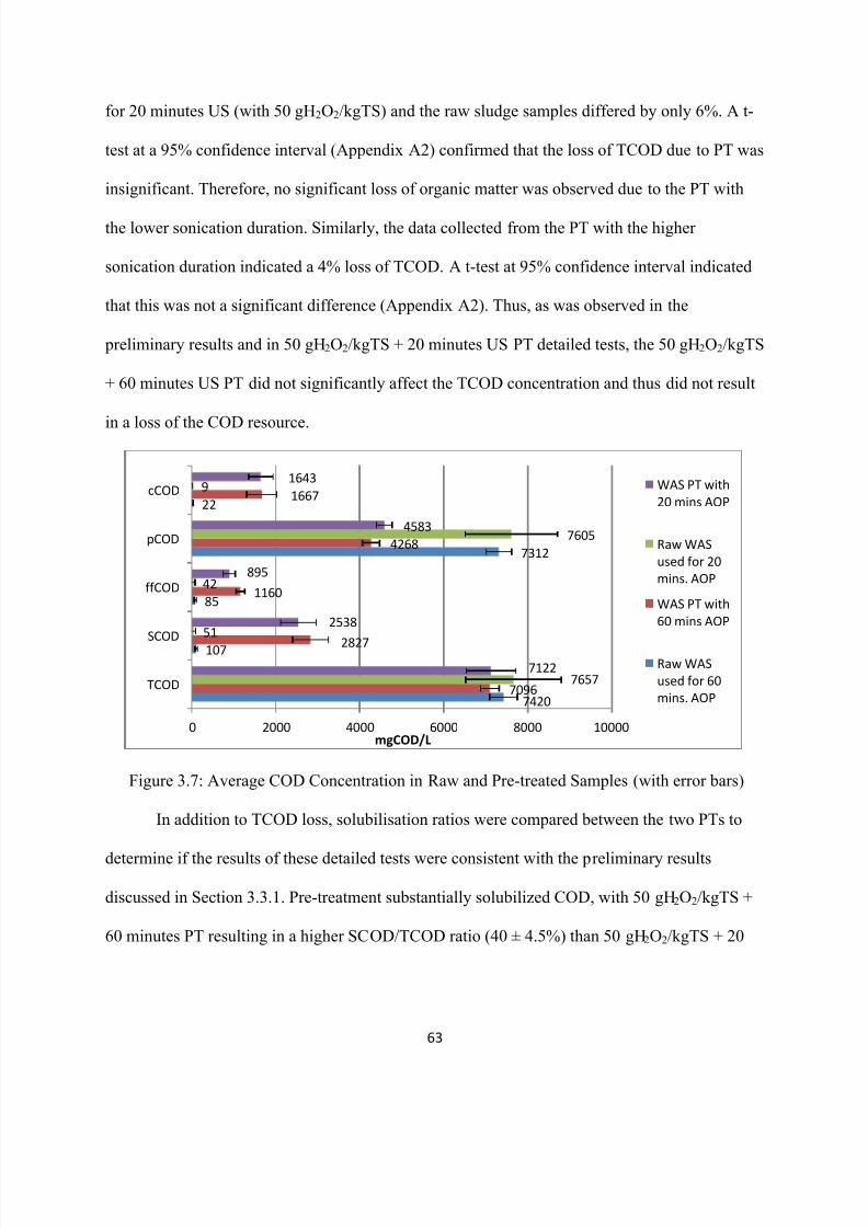
8/10/2019 Joshi Priyanka
http://slidepdf.com/reader/full/joshi-priyanka 79/166
63
for 20 minutes US (with 50 gH2O2/kgTS) and the raw sludge samples differed by only 6%. A t-
test at a 95% confidence interval (Appendix A2) confirmed that the loss of TCOD due to PT was
insignificant. Therefore, no significant loss of organic matter was observed due to the PT with
the lower sonication duration. Similarly, the data collected from the PT with the higher
sonication duration indicated a 4% loss of TCOD. A t-test at 95% confidence interval indicated
that this was not a significant difference (Appendix A2). Thus, as was observed in the
preliminary results and in 50 gH2O2/kgTS + 20 minutes US PT detailed tests, the 50 gH2O2/kgTS
+ 60 minutes US PT did not significantly affect the TCOD concentration and thus did not result
in a loss of the COD resource.
Figure 3.7: Average COD Concentration in Raw and Pre-treated Samples (with error bars)
In addition to TCOD loss, solubilisation ratios were compared between the two PTs to
determine if the results of these detailed tests were consistent with the preliminary results
discussed in Section 3.3.1. Pre-treatment substantially solubilized COD, with 50 gH2O2/kgTS +
60 minutes PT resulting in a higher SCOD/TCOD ratio (40 ± 4.5%) than 50 gH2O2/kgTS + 20
7420
107
85
7312
22
7096
2827
1160
4268
1667
7657
51
42
7605
9
7122
2538
895
4583
1643
0 2000 4000 6000 8000 10000
TCOD
SCOD
ffCOD
pCOD
cCOD
mgCOD/L
WAS PT with
20 mins AOP
Raw WAS
used for 20
mins. AOP
WAS PT with
60 mins AOP
Raw WAS
used for 60
mins. AOP

8/10/2019 Joshi Priyanka
http://slidepdf.com/reader/full/joshi-priyanka 80/166
64
minutes PT (33 ± 0.60 %). Hence the solubilisation ratios achieved with both PTs were similar to
the results obtained in the preliminary tests.
The colloidal and truly soluble COD fractions were also compared between the two PTs
to determine if PT resulted in a change in these fractions. From Figure 3.7 it can be seen that
both the cCOD and ffCOD concentrations increased due to PT. The cCOD fractions increased by
21 and 24% for the 20 and 60 minute US AOPs, respectively. The ffCOD fractions increased by
11 and 15% for the 20 and 60 minutes US AOPs, respectively. A t-test at 95% confidence
interval (Appendix A2) indicated that ffCOD and cCOD concentrations generated in both PTs
were significantly different from their respective feeds. This increase was in agreement with
Kianmehr, (2010), as discussed in Section 3.3.1. Therefore, both PTs resulted in an increase in
colloids and truly soluble materials as was expected based on the SCOD/TCOD results.
Colloidal and truly soluble COD fractions were also compared between the two PTs to
assess whether the level of PT affected the distribution of these fractions in WAS (Figure 3.7).
From Figure 3.7 it can be seen that the ffCOD and cCOD concentrations resulting from the AOP
with 60 minutes of sonication were greater than the AOP with 20 minutes of sonication. The
average ffCOD/TCOD fractions for the sludges generated by the 20 minutes and 60 minutes US
PT (each with 50 gH2O2/kgTS ) were 11.7 ± 0.7% and 16.0 ± 0.7%, respectively whereas the
average cCOD/TCOD fractions were 21.4 ± 0.7% and 24 ± 4%, respectively. In addition, the
ffCOD/cCOD ratio increased from 55 ± 4% to 72 ± 14% with an increase in sonication duration.
Therefore, the AOP with the 60 minutes of sonication was more effective in solubilising
particulates into truly soluble COD. On the basis of these results it was hypothesized that the PT
with 60 minutes of sonication may generate more readily biodegradable COD than the PT with
20 minutes of sonication as a result of the higher ffCOD concentration.
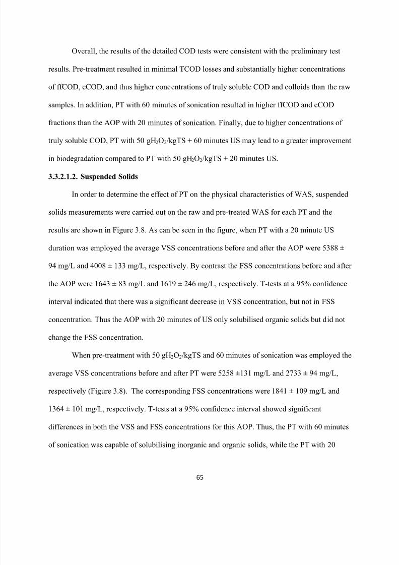
8/10/2019 Joshi Priyanka
http://slidepdf.com/reader/full/joshi-priyanka 81/166
65
Overall, the results of the detailed COD tests were consistent with the preliminary test
results. Pre-treatment resulted in minimal TCOD losses and substantially higher concentrations
of ffCOD, cCOD, and thus higher concentrations of truly soluble COD and colloids than the raw
samples. In addition, PT with 60 minutes of sonication resulted in higher ffCOD and cCOD
fractions than the AOP with 20 minutes of sonication. Finally, due to higher concentrations of
truly soluble COD, PT with 50 gH2O2/kgTS + 60 minutes US may lead to a greater improvement
in biodegradation compared to PT with 50 gH2O2/kgTS + 20 minutes US.
3.3.2.1.2. Suspended Solids
In order to determine the effect of PT on the physical characteristics of WAS, suspended
solids measurements were carried out on the raw and pre-treated WAS for each PT and the
results are shown in Figure 3.8. As can be seen in the figure, when PT with a 20 minute US
duration was employed the average VSS concentrations before and after the AOP were 5388 ±
94 mg/L and 4008 ± 133 mg/L, respectively. By contrast the FSS concentrations before and after
the AOP were 1643 ± 83 mg/L and 1619 ± 246 mg/L, respectively. T-tests at a 95% confidence
interval indicated that there was a significant decrease in VSS concentration, but not in FSS
concentration. Thus the AOP with 20 minutes of US only solubilised organic solids but did not
change the FSS concentration.
When pre-treatment with 50 gH2O2/kgTS and 60 minutes of sonication was employed the
average VSS concentrations before and after PT were 5258 ±131 mg/L and 2733 ± 94 mg/L,
respectively (Figure 3.8). The corresponding FSS concentrations were 1841 ± 109 mg/L and
1364 ± 101 mg/L, respectively. T-tests at a 95% confidence interval showed significant
differences in both the VSS and FSS concentrations for this AOP. Thus, the PT with 60 minutes
of sonication was capable of solubilising inorganic and organic solids, while the PT with 20
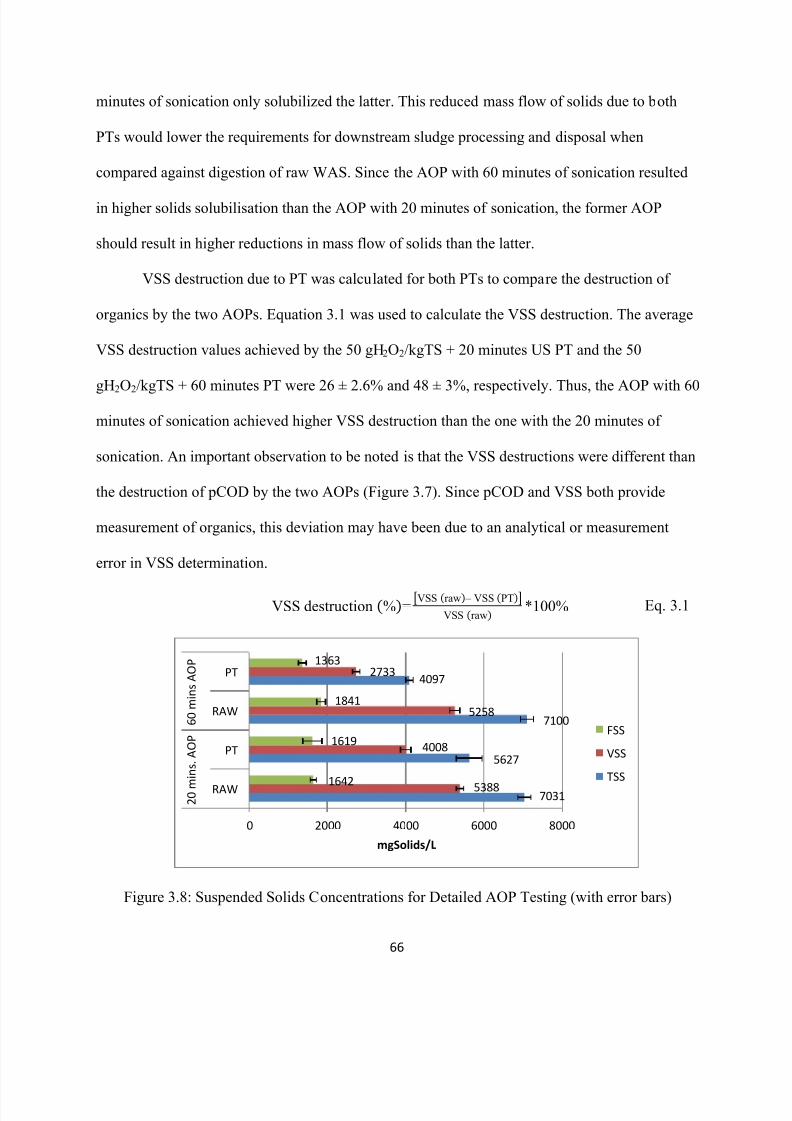
8/10/2019 Joshi Priyanka
http://slidepdf.com/reader/full/joshi-priyanka 82/166
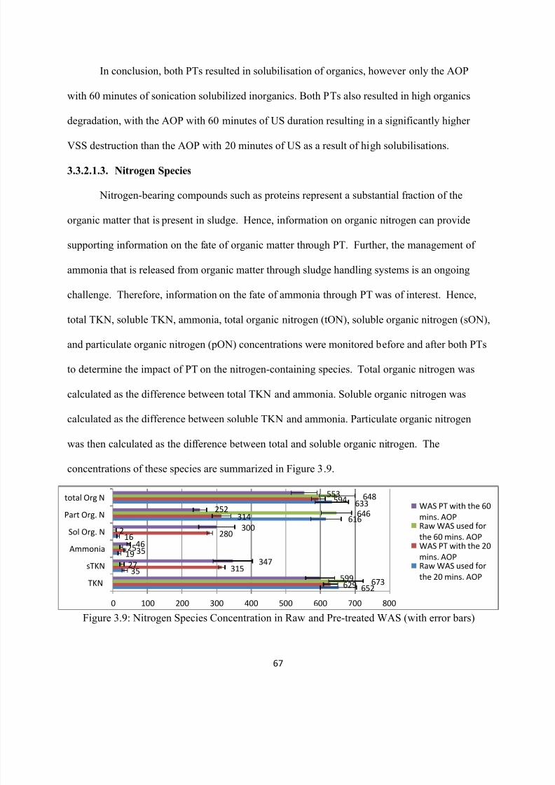
8/10/2019 Joshi Priyanka
http://slidepdf.com/reader/full/joshi-priyanka 83/166
67
In conclusion, both PTs resulted in solubilisation of organics, however only the AOP
with 60 minutes of sonication solubilized inorganics. Both PTs also resulted in high organics
degradation, with the AOP with 60 minutes of US duration resulting in a significantly higher
VSS destruction than the AOP with 20 minutes of US as a result of high solubilisations.
3.3.2.1.3. Nitrogen Species
Nitrogen-bearing compounds such as proteins represent a substantial fraction of the
organic matter that is present in sludge. Hence, information on organic nitrogen can provide
supporting information on the fate of organic matter through PT. Further, the management of
ammonia that is released from organic matter through sludge handling systems is an ongoing
challenge. Therefore, information on the fate of ammonia through PT was of interest. Hence,
total TKN, soluble TKN, ammonia, total organic nitrogen (tON), soluble organic nitrogen (sON),
and particulate organic nitrogen (pON) concentrations were monitored before and after both PTs
to determine the impact of PT on the nitrogen-containing species. Total organic nitrogen was
calculated as the difference between total TKN and ammonia. Soluble organic nitrogen was
calculated as the difference between soluble TKN and ammonia. Particulate organic nitrogen
was then calculated as the difference between total and soluble organic nitrogen. The
concentrations of these species are summarized in Figure 3.9.
Figure 3.9: Nitrogen Species Concentration in Raw and Pre-treated WAS (with error bars)
652
35
19
16
616
633
629
315
35
280
314
594
673
27
25
2
646
648
599
347
46
300
252
553
0 100 200 300 400 500 600 700 800
TKN
sTKN
Ammonia
Sol Org. N
Part Org. N
total Org NWAS PT with the 60
mins. AOPRaw WAS used for
the 60 mins. AOP
WAS PT with the 20mins. AOPRaw WAS used for
the 20 mins. AOP
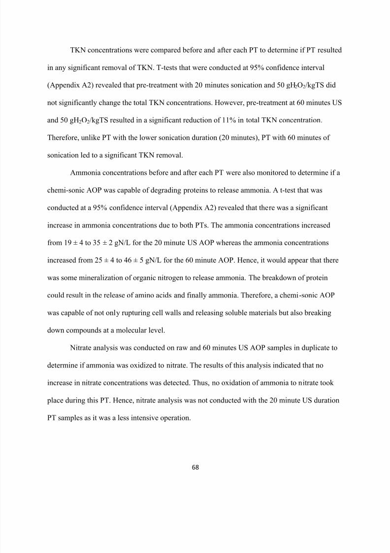
8/10/2019 Joshi Priyanka
http://slidepdf.com/reader/full/joshi-priyanka 84/166
68
TKN concentrations were compared before and after each PT to determine if PT resulted
in any significant removal of TKN. T-tests that were conducted at 95% confidence interval
(Appendix A2) revealed that pre-treatment with 20 minutes sonication and 50 gH2O2/kgTS did
not significantly change the total TKN concentrations. However, pre-treatment at 60 minutes US
and 50 gH2O2/kgTS resulted in a significant reduction of 11% in total TKN concentration.
Therefore, unlike PT with the lower sonication duration (20 minutes), PT with 60 minutes of
sonication led to a significant TKN removal.
Ammonia concentrations before and after each PT were also monitored to determine if a
chemi-sonic AOP was capable of degrading proteins to release ammonia. A t-test that was
conducted at a 95% confidence interval (Appendix A2) revealed that there was a significant
increase in ammonia concentrations due to both PTs. The ammonia concentrations increased
from 19 ± 4 to 35 ± 2 gN/L for the 20 minute US AOP whereas the ammonia concentrations
increased from 25 ± 4 to 46 ± 5 gN/L for the 60 minute AOP. Hence, it would appear that there
was some mineralization of organic nitrogen to release ammonia. The breakdown of protein
could result in the release of amino acids and finally ammonia. Therefore, a chemi-sonic AOP
was capable of not only rupturing cell walls and releasing soluble materials but also breaking
down compounds at a molecular level.
Nitrate analysis was conducted on raw and 60 minutes US AOP samples in duplicate to
determine if ammonia was oxidized to nitrate. The results of this analysis indicated that no
increase in nitrate concentrations was detected. Thus, no oxidation of ammonia to nitrate took
place during this PT. Hence, nitrate analysis was not conducted with the 20 minute US duration
PT samples as it was a less intensive operation.
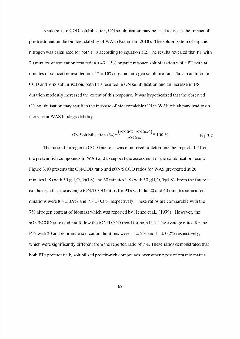
8/10/2019 Joshi Priyanka
http://slidepdf.com/reader/full/joshi-priyanka 85/166
69
Analogous to COD solubilisation, ON solubilisation may be used to assess the impact of
pre-treatment on the biodegradability of WAS (Kianmehr, 2010). The solubilisation of organic
nitrogen was calculated for both PTs according to equation 3.2. The results revealed that PT with
20 minutes of sonication resulted in a 43 ± 5% organic nitrogen solubilisation while PT with 60
minutes of sonication resulted in a 47 ± 10% organic nitrogen solubilisation. Thus in addition to
COD and VSS solubilisation, both PTs resulted in ON solubilisation and an increase in US
duration modestly increased the extent of this response. It was hypothesized that the observed
ON solubilisation may result in the increase of biodegradable ON in WAS which may lead to an
increase in WAS biodegradability.
olubilisation sO P – sO raw
pO raw 100
The ratio of nitrogen to COD fractions was monitored to determine the impact of PT on
the protein rich compounds in WAS and to support the assessment of the solubilisation result.
Figure 3.10 presents the ON/COD ratio and sON/SCOD ratios for WAS pre-treated at 20
minutes US (with 50 gH2O2/kgTS) and 60 minutes US (with 50 gH2O2/kgTS). From the figure it
can be seen that the average tON/TCOD ratios for PTs with the 20 and 60 minutes sonication
durations were 8.4 ± 0.9% and 7.8 ± 0.3 % respectively. These ratios are comparable with the
7% nitrogen content of biomass which was reported by Henze et al., (1999). However, the
sON/SCOD ratios did not follow the tON/TCOD trend for both PTs. The average ratios for the
PTs with 20 and 60 minute sonication durations were 11 ± 2% and 11 ± 0.2% respectively,
which were significantly different from the reported ratio of 7%. These ratios demonstrated that
both PTs preferentially solubilised protein-rich compounds over other types of organic matter.
Eq. 3.2
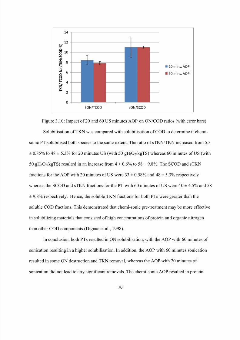
8/10/2019 Joshi Priyanka
http://slidepdf.com/reader/full/joshi-priyanka 86/166
70
Figure 3.10: Impact of 20 and 60 US minutes AOP on ON/COD ratios (with error bars)
Solubilisation of TKN was compared with solubilisation of COD to determine if chemi-
sonic PT solubilised both species to the same extent. The ratio of sTKN/TKN increased from 5.3
± 0.85% to 48 ± 5.3% for 20 minutes US (with 50 gH2O2/kgTS) whereas 60 minutes of US (with
50 gH2O2/kgTS) resulted in an increase from 4 ± 0.6% to 58 ± 9.8%. The SCOD and sTKN
fractions for the AOP with 20 minutes of US were 33 ± 0.58% and 48 ± 5.3% respectively
whereas the SCOD and sTKN fractions for the PT with 60 minutes of US were 40 ± 4.5% and 58
± 9.8% respectively. Hence, the soluble TKN fractions for both PTs were greater than the
soluble COD fractions. This demonstrated that chemi-sonic pre-treatment may be more effective
in solubilizing materials that consisted of high concentrations of protein and organic nitrogen
than other COD components (Dignac et al., 1998).
In conclusion, both PTs resulted in ON solubilisation, with the AOP with 60 minutes of
sonication resulting in a higher solubilisation. In addition, the AOP with 60 minutes sonication
resulted in some ON destruction and TKN removal, whereas the AOP with 20 minutes of
sonication did not lead to any significant removals. The chemi-sonic AOP resulted in protein
0
2
4
6
8
10
12
14
tON/TCOD sON/SCOD
T K N / T C O D % ( s T K N / S C O D % )
20 mins. AOP
60 mins. AOP
8/10/2019 Joshi Priyanka
http://slidepdf.com/reader/full/joshi-priyanka 87/166
71
degradation, causing an increase in ammonia concentration. Both PTs were more effective in
solubilising TKN particulates than COD particulates.
In summary, all pre-treatments of waste activated sludge examined in this study led to
solubilisation of COD. Further, all the AOPs employed in this study resulted in higher
solubilisation than the individuals PT. Both AOPs employed in the detailed study significantly
solubilised COD while conserving the TCOD, with the 60 minutes AOP resulting in the highest
solubilisation. Moreover, the AOP with the lower sonication duration (20 minutes) preferentially
solubilized organics while the AOP with the higher US duration (60 minutes) solubilized both
organic and inorganic solids. The 60 minute AOP resulted in higher VSS destruction than the 20
minute AOP. T the PT with 60 minutes of US resulted in significant ON destruction, while the
PT with 20 minutes of US did not. Both PTs solubilized ON and the solubilisation of this organic
matter was greater than that of other types of organic matter.
3.3.3. Anaerobic Membrane Bioreactor Operation
This portion of the study is sought to assess the impact of two different levels of the AOP
PT on the anaerobic biodegradability of WAS. Biodegradability of WAS was evaluated by
treating the WAS in an AnMBR. This section presents the results of anaerobic digestion of raw
and PT WAS in the AnMBR. The stability of the AnMBR was measured by monitoring the pH
and the VFA/Alk ratio while the overall performance of the AnMBR was measured in terms of
COD, VSS, and ON destruction.
3.3.3.1. pH and VFA/Alk Ratio for AnMBR
It was hypothesized that PT of the WAS would increase the biodegradability of the WAS
and hence stability with respect to pH excursions was a potential operational concern. The pH of
the waste and permeate streams was monitored for all phases of AnMBR operation to assess the
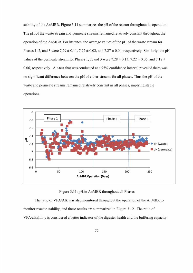
8/10/2019 Joshi Priyanka
http://slidepdf.com/reader/full/joshi-priyanka 88/166
72
stability of the AnMBR. Figure 3.11 summarizes the pH of the reactor throughout its operation.
The pH of the waste stream and permeate streams remained relatively constant throughout the
operation of the AnMBR. For instance, the average values of the pH of the waste stream for
Phases 1, 2, and 3 were 7.29 ± 0.11, 7.22 ± 0.02, and 7.27 ± 0.04, respectively. Similarly, the pH
values of the permeate stream for Phases 1, 2, and 3 were 7.28 ± 0.13, 7.22 ± 0.06, and 7.18 ±
0.06, respectively. A t-test that was conducted at a 95% confidence interval revealed there was
no significant difference between the pH of either streams for all phases. Thus the pH of the
waste and permeate streams remained relatively constant in all phases, implying stable
operations.
Figure 3.11: pH in AnMBR throughout all Phases
The ratio of VFA/Alk was also monitored throughout the operation of the AnMBR to
monitor reactor stability, and these results are summarized in Figure 3.12. The ratio of
VFA/alkalinity is considered a better indicator of the digester health and the buffering capacity
6.6
6.8
7
7.2
7.4
7.6
7.8
8
0 50 100 150 200 250
p H
AnMBR Operation (Days)
pH (waste)
pH (permeate)
Phase 1 Phase 2 Phase 3
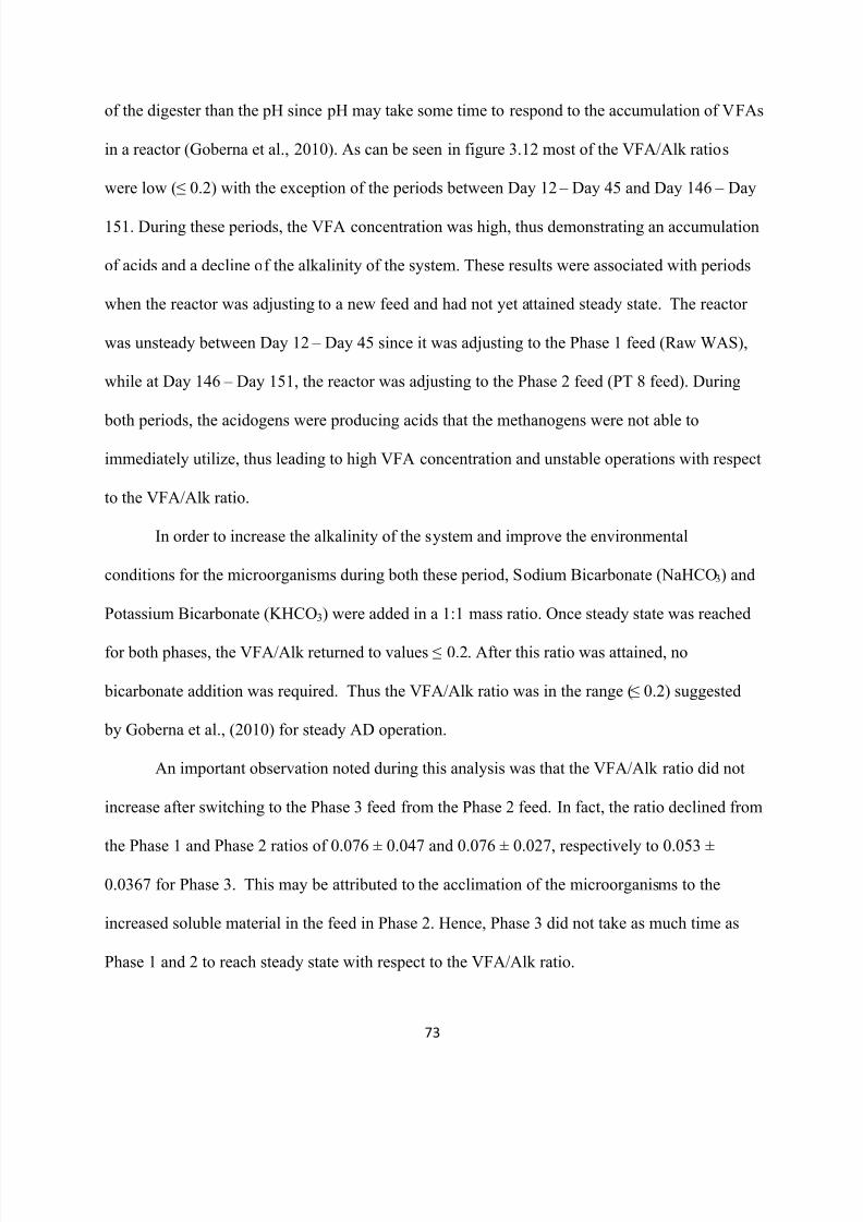
8/10/2019 Joshi Priyanka
http://slidepdf.com/reader/full/joshi-priyanka 89/166
73
of the digester than the pH since pH may take some time to respond to the accumulation of VFAs
in a reactor (Goberna et al., 2010). As can be seen in figure 3.12 most of the VFA/Alk ratios
were low (≤ 0.2) with the exception of the periods between Day 12 – Day 45 and Day 146 – Day
151. During these periods, the VFA concentration was high, thus demonstrating an accumulation
of acids and a decline of the alkalinity of the system. These results were associated with periods
when the reactor was adjusting to a new feed and had not yet attained steady state. The reactor
was unsteady between Day 12 – Day 45 since it was adjusting to the Phase 1 feed (Raw WAS),
while at Day 146 – Day 151, the reactor was adjusting to the Phase 2 feed (PT 8 feed). During
both periods, the acidogens were producing acids that the methanogens were not able to
immediately utilize, thus leading to high VFA concentration and unstable operations with respect
to the VFA/Alk ratio.
In order to increase the alkalinity of the system and improve the environmental
conditions for the microorganisms during both these period, Sodium Bicarbonate (NaHCO3) and
Potassium Bicarbonate (KHCO3) were added in a 1:1 mass ratio. Once steady state was reached
for both phases, the FA/Alk returned to values ≤ 0.2. After this ratio was attained, no
bicarbonate addition was required. Thus the VFA/Alk ratio was in the range (≤ 0.2) suggested
by Goberna et al., (2010) for steady AD operation.
An important observation noted during this analysis was that the VFA/Alk ratio did not
increase after switching to the Phase 3 feed from the Phase 2 feed. In fact, the ratio declined from
the Phase 1 and Phase 2 ratios of 0.076 ± 0.047 and 0.076 ± 0.027, respectively to 0.053 ±
0.0367 for Phase 3. This may be attributed to the acclimation of the microorganisms to the
increased soluble material in the feed in Phase 2. Hence, Phase 3 did not take as much time as
Phase 1 and 2 to reach steady state with respect to the VFA/Alk ratio.
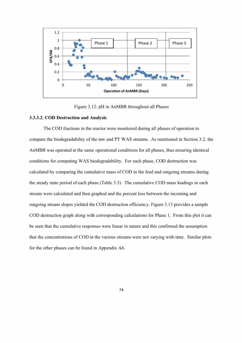
8/10/2019 Joshi Priyanka
http://slidepdf.com/reader/full/joshi-priyanka 90/166
74
Figure 3.12: pH in AnMBR throughout all Phases
3.3.3.2. COD Destruction and Analysis
The COD fractions in the reactor were monitored during all phases of operation to
compare the biodegradability of the raw and PT WAS streams. As mentioned in Section 3.2, the
AnMBR was operated at the same operational conditions for all phases, thus ensuring identical
conditions for comparing WAS biodegradability. For each phase, COD destruction was
calculated by comparing the cumulative mass of COD in the feed and outgoing streams during
the steady state period of each phase (Table 3.3). The cumulative COD mass loadings in each
stream were calculated and then graphed and the percent loss between the incoming and
outgoing stream slopes yielded the COD destruction efficiency. Figure 3.13 provides a sample
COD destruction graph along with corresponding calculations for Phase 1. From this plot it can
be seen that the cumulative responses were linear in nature and this confirmed the assumption
that the concentrations of COD in the various streams were not varying with time. Similar plots
for the other phases can be found in Appendix A6.
0
0.2
0.4
0.6
0.8
1
1.2
0 50 100 150 200 250
V F
A / A l k
Operation of AnMBR (Days)
Phase 1 Phase 3Phase 2
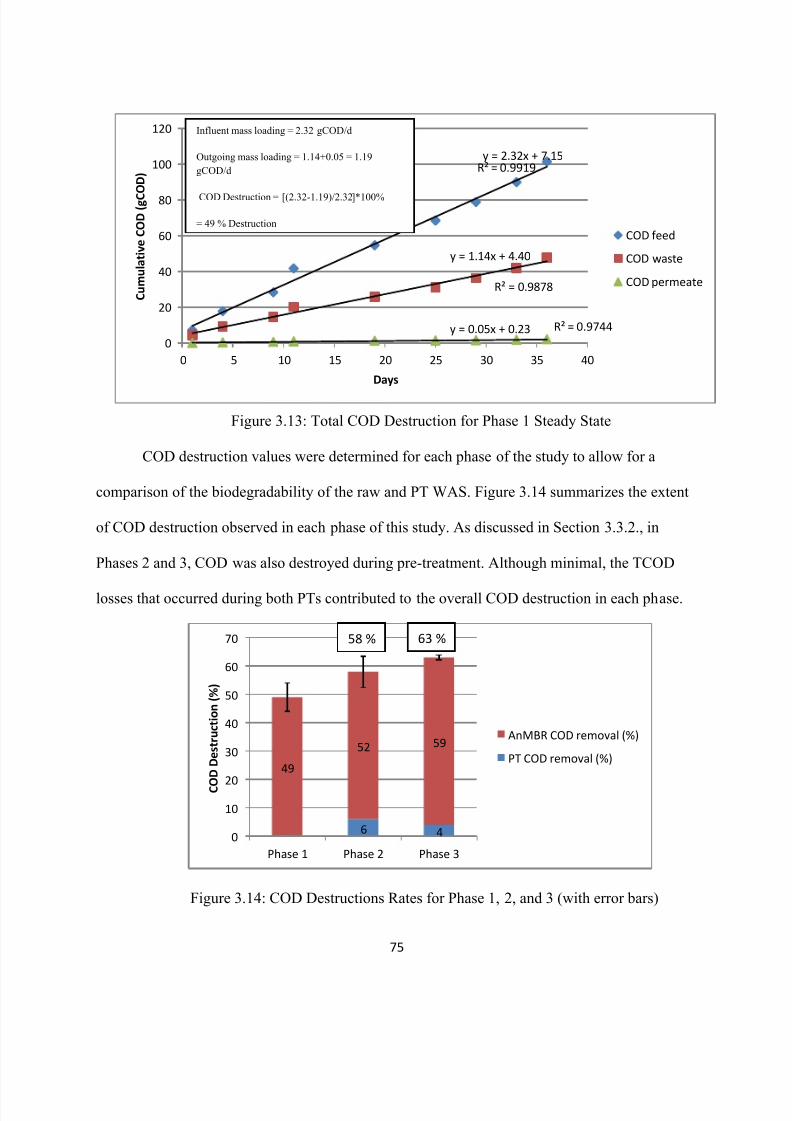
8/10/2019 Joshi Priyanka
http://slidepdf.com/reader/full/joshi-priyanka 91/166
75
Figure 3.13: Total COD Destruction for Phase 1 Steady State
COD destruction values were determined for each phase of the study to allow for a
comparison of the biodegradability of the raw and PT WAS. Figure 3.14 summarizes the extent
of COD destruction observed in each phase of this study. As discussed in Section 3.3.2., in
Phases 2 and 3, COD was also destroyed during pre-treatment. Although minimal, the TCOD
losses that occurred during both PTs contributed to the overall COD destruction in each phase.
Figure 3.14: COD Destructions Rates for Phase 1, 2, and 3 (with error bars)
6 4
49
52 59
0
10
20
30
40
50
60
70
Phase 1 Phase 2 Phase 3
C O
D D e s t r u c t i o n ( % )
AnMBR COD removal (%)
PT COD removal (%)
58 % 63 %
y = 2.32x + 7.15R² = 0.9919
y = 1.14x + 4.40
R² = 0.9878
y = 0.05x + 0.23 R² = 0.9744
0
20
40
60
80
100
120
0 5 10 15 20 25 30 35 40
C u m u l a t i v e C O D ( g C
O D )
Days
COD feed
COD waste
COD permeate
Influent mass loading = 2.32 gCOD/d
Outgoing mass loading = 1.14+0.05 = 1.19
gCOD/d
COD Destruction = [(2.32-1.19)/2.32]*100%
= 49 % Destruction
8/10/2019 Joshi Priyanka
http://slidepdf.com/reader/full/joshi-priyanka 92/166
76
As it can be seen from Figure 3.14, Phase 1 resulted in 49% COD destruction, while
Phases 2 and 3 resulted in increased overall COD destruction values of 58 and 63%, respectively.
Hence, when compared to operation without PT the overall performance improved from Phase 1
to Phase 2 by an increment of 9% while Phase 3 resulted in an increase by 14% with respect to
Phase 1. In terms of digester performance, it is seen that the COD destruction increased from 49
to 52% after switching the feed from raw to Phase 2 PT WAS. The COD destruction in the
digester further improved by an increment of 7% after changing the PT conditions from Phase 2
to Phase 3. It has been previously shown that anaerobic digestion at an SRT of 20 days will
result in the destruction of the majority of the biodegradable fraction of sludge (Szeinbaum,
2009). Hence, it appears that both PTs were able to convert some non-biodegradable COD to
biodegradable COD, which resulted in an improvement in the ultimate biodegradability of WAS.
Therefore pre-treatment of WAS by the AOPs increased the biodegradation of WAS, with the
highest destruction observed with the AOP involving the greatest sonication duration and
peroxide dose.
The concentrations of pCOD, SCOD, ffCOD, and cCOD were monitored during the
steady state operation of the AnMBR to obtain insight into the fate of these materials in the
digester. It was hypothesized that an improved understanding of the behaviour of these materials
would provide insight into the biodegradability of the soluble and colloidal fractions that were
generated in PT. Figure 3.15 presents the concentrations of these COD species in the AnMBR
waste stream for each phase. From Figure 3.15 it can be seen that the concentrations of all COD
species decreased as the level of PT intensity increased (i.e. Phase 3<Phase 2< Phase 1). The
average pCOD and SCOD concentrations were 15 and 23% lower in Phase 2 than Phase 1. These
values were further decreased by 5% and 26% in Phase 3. ANOVA tests revealed that there was
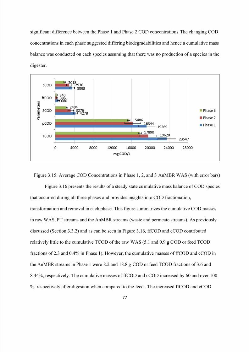
8/10/2019 Joshi Priyanka
http://slidepdf.com/reader/full/joshi-priyanka 93/166
77
23547
19269
4278
680
3598
19620
16344
3276
386
2936
17890
15486
2404
340
2018
0 4000 8000 12000 16000 20000 24000 28000
TCOD
pCOD
SCOD
ffCOD
cCOD
mg COD/L
P a r a m e t e r s
Phase 3
Phase 2
Phase 1
significant difference between the Phase 1 and Phase 2 COD concentrations. The changing COD
concentrations in each phase suggested differing biodegradabilities and hence a cumulative mass
balance was conducted on each species assuming that there was no production of a species in the
digester.
Figure 3.15: Average COD Concentrations in Phase 1, 2, and 3 AnMBR WAS (with error bars)
Figure 3.16 presents the results of a steady state cumulative mass balance of COD species
that occurred during all three phases and provides insights into COD fractionation,
transformation and removal in each phase. This figure summarizes the cumulative COD masses
in raw WAS, PT streams and the AnMBR streams (waste and permeate streams). As previously
discussed (Section 3.3.2) and as can be seen in Figure 3.16, ffCOD and cCOD contributed
relatively little to the cumulative TCOD of the raw WAS (5.1 and 0.9 g COD or feed TCOD
fractions of 2.3 and 0.4% in Phase 1). However, the cumulative masses of ffCOD and cCOD in
the AnMBR streams in Phase 1 were 8.2 and 18.8 g COD or feed TCOD fractions of 3.6 and
8.44%, respectively. The cumulative masses of ffCOD and cCOD increased by 60 and over 100
%, respectively after digestion when compared to the feed. The increased ffCOD and cCOD
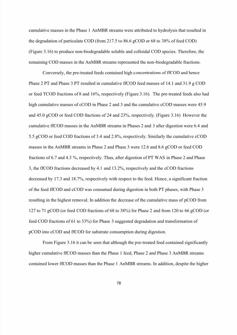
8/10/2019 Joshi Priyanka
http://slidepdf.com/reader/full/joshi-priyanka 94/166
78
cumulative masses in the Phase 1 AnMBR streams were attributed to hydrolysis that resulted in
the degradation of particulate COD (from 217.5 to 86.6 gCOD or 68 to 38% of feed COD)
(Figure 3.16) to produce non-biodegradable soluble and colloidal COD species. Therefore, the
remaining COD masses in the AnMBR streams represented the non-biodegradable fractions.
Conversely, the pre-treated feeds contained high concentrations of ffCOD and hence
Phase 2 PT and Phase 3 PT resulted in cumulative ffCOD feed masses of 14.1 and 31.9 g COD
or feed TCOD fractions of 8 and 16%, respectively (Figure 3.16). The pre-treated feeds also had
high cumulative masses of cCOD in Phase 2 and 3 and the cumulative cCOD masses were 45.9
and 45.0 gCOD or feed COD fractions of 24 and 23%, respectively. (Figure 3.16) However the
cumulative ffCOD masses in the AnMBR streams in Phases 2 and 3 after digestion were 6.4 and
5.5 gCOD or feed COD fractions of 3.4 and 2.8%, respectively. Similarly the cumulative cCOD
masses in the AnMBR streams in Phase 2 and Phase 3 were 12.6 and 8.6 gCOD or feed COD
fractions of 6.7 and 4.3 %, respectively. Thus, after digestion of PT WAS in Phase 2 and Phase
3, the ffCOD fractions decreased by 4.1 and 13.2%, respectively and the cCOD fractions
decreased by 17.3 and 18.7%, respectively with respect to the feed. Hence, a significant fraction
of the feed ffCOD and cCOD was consumed during digestion in both PT phases, with Phase 3
resulting in the highest removal. In addition the decrease of the cumulative mass of pCOD from
127 to 71 gCOD (or feed COD fractions of 68 to 38%) for Phase 2 and from 120 to 66 gCOD (or
feed COD fractions of 61 to 33%) for Phase 3 suggested degradation and transformation of
pCOD into cCOD and ffCOD for substrate consumption during digestion.
From Figure 3.16 it can be seen that although the pre-treated feed contained significantly
higher cumulative ffCOD masses than the Phase 1 feed, Phase 2 and Phase 3 AnMBR streams
contained lower ffCOD masses than the Phase 1 AnMBR streams. In addition, despite the higher
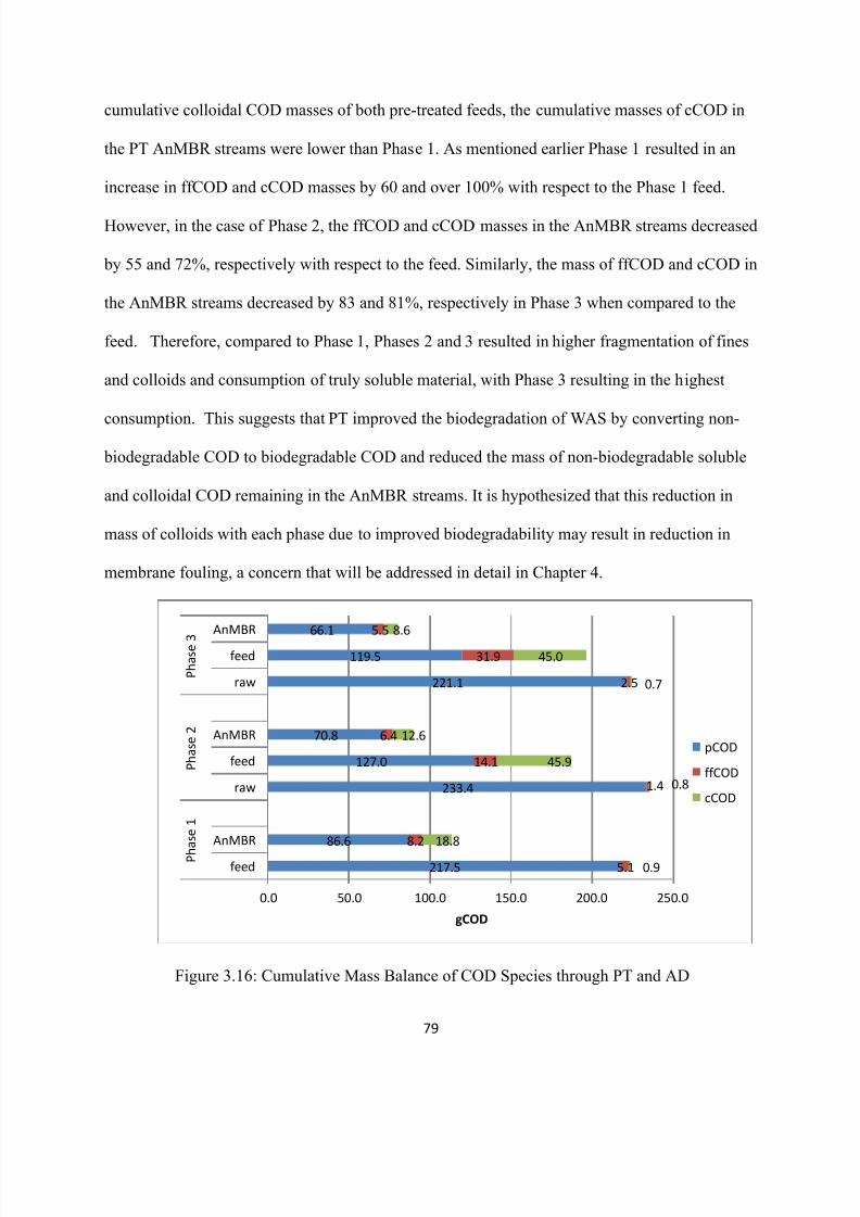
8/10/2019 Joshi Priyanka
http://slidepdf.com/reader/full/joshi-priyanka 95/166
79
cumulative colloidal COD masses of both pre-treated feeds, the cumulative masses of cCOD in
the PT AnMBR streams were lower than Phase 1. As mentioned earlier Phase 1 resulted in an
increase in ffCOD and cCOD masses by 60 and over 100% with respect to the Phase 1 feed.
However, in the case of Phase 2, the ffCOD and cCOD masses in the AnMBR streams decreased
by 55 and 72%, respectively with respect to the feed. Similarly, the mass of ffCOD and cCOD in
the AnMBR streams decreased by 83 and 81%, respectively in Phase 3 when compared to the
feed. Therefore, compared to Phase 1, Phases 2 and 3 resulted in higher fragmentation of fines
and colloids and consumption of truly soluble material, with Phase 3 resulting in the highest
consumption. This suggests that PT improved the biodegradation of WAS by converting non-
biodegradable COD to biodegradable COD and reduced the mass of non-biodegradable soluble
and colloidal COD remaining in the AnMBR streams. It is hypothesized that this reduction in
mass of colloids with each phase due to improved biodegradability may result in reduction in
membrane fouling, a concern that will be addressed in detail in Chapter 4.
Figure 3.16: Cumulative Mass Balance of COD Species through PT and AD
217.5
86.6
233.4
127.0
70.8
221.1
119.5
66.1
5.1
8.2
1.4
14.1
6.4
2.5
31.9
5.5
0.9
18.8
0.8
45.9
12.6
0.7
45.0
8.6
0.0 50.0 100.0 150.0 200.0 250.0
feed
AnMBR
raw
feed
AnMBR
raw
feed
AnMBR
P h
a s e 1
P h a s e 2
P h a s e 3
gCOD
pCOD
ffCOD
cCOD
8/10/2019 Joshi Priyanka
http://slidepdf.com/reader/full/joshi-priyanka 96/166
80
Permeate ffCOD concentrations were also monitored during the operation of the AnMBR
to determine permeate quality that might impact upon downstream operations in a wastewater
treatment plant. Figure 3.17 summarizes the permeate ffCOD concentrations for Phases 1, 2, and
3. From this figure it can be seen that low and comparable ffCOD concentrations of 151-166
mg/L were observed for all phases. The permeate concentrations were compared and found to be
not statistically indifferent. Therefore PT did not result in any significant change in permeate
quality.
Figure 3.17: Average Permeate ffCOD Concentrations for all Phases (with error bars)
3.3.3.3. Solids Destruction
The behaviour of suspended solids was examined as an additional indicator of the
performance of the AnMBR. For each phase, VSS destruction was calculated by comparing the
cumulative mass of VSS in the feed and outgoing streams. Since the permeate was solids-free,
only the waste stream was used in the cumulative analysis. Once the cumulative VSS mass
loading in the streams were calculated, they were plotted versus time and the difference between
the incoming and outgoing stream slopes was employed to calculate the VSS destruction
efficiency. Figure 3.18 provides a sample VSS mass loading graph along with corresponding
calculations for Phase 1. VSS data for all other phases can be found in Appendix A7. From
161
166
151
0 50 100 150 200 250
Phase 1
Phase 2
Phase 3
mg COD/L
P h a s e s
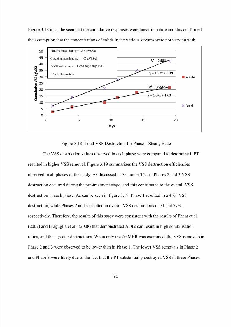
8/10/2019 Joshi Priyanka
http://slidepdf.com/reader/full/joshi-priyanka 97/166
81
Figure 3.18 it can be seen that the cumulative responses were linear in nature and this confirmed
the assumption that the concentrations of solids in the various streams were not varying with
time.
Figure 3.16: Total VSS destruction for Phase 1 Steady State
Figure 3.18: Total VSS Destruction for Phase 1 Steady State
The VSS destruction values observed in each phase were compared to determine if PT
resulted in higher VSS removal. Figure 3.19 summarizes the VSS destruction efficiencies
observed in all phases of the study. As discussed in Section 3.3.2., in Phases 2 and 3 VSS
destruction occurred during the pre-treatment stage, and this contributed to the overall VSS
destruction in each phase. As can be seen in figure 3.19, Phase 1 resulted in a 46% VSS
destruction, while Phases 2 and 3 resulted in overall VSS destructions of 71 and 77%,
respectively. Therefore, the results of this study were consistent with the results of Pham et al.
(2007) and Braguglia et al. |(2008) that demonstrated AOPs can result in high solubilisation
ratios, and thus greater destructions. When only the AnMBR was examined, the VSS removals in
Phase 2 and 3 were observed to be lower than in Phase 1. The lower VSS removals in Phase 2
and Phase 3 were likely due to the fact that the PT substantially destroyed VSS in these Phases.
y = 1.07x + 1.63
R² = 0.9861
y = 1.97x + 5.39
R² = 0.988
0
5
10
15
20
25
30
35
40
45
50
0 5 10 15 20
C u m u l a t i v e V S S ( g V S S )
Days
Waste
Feed
Influent mass loading = 1.97 gVSS/d
Outgoing mass loading = 1.07 gVSS/d
VSS Destruction = [(1.97-1.07)/1.97]*100%
= 46 % Destruction
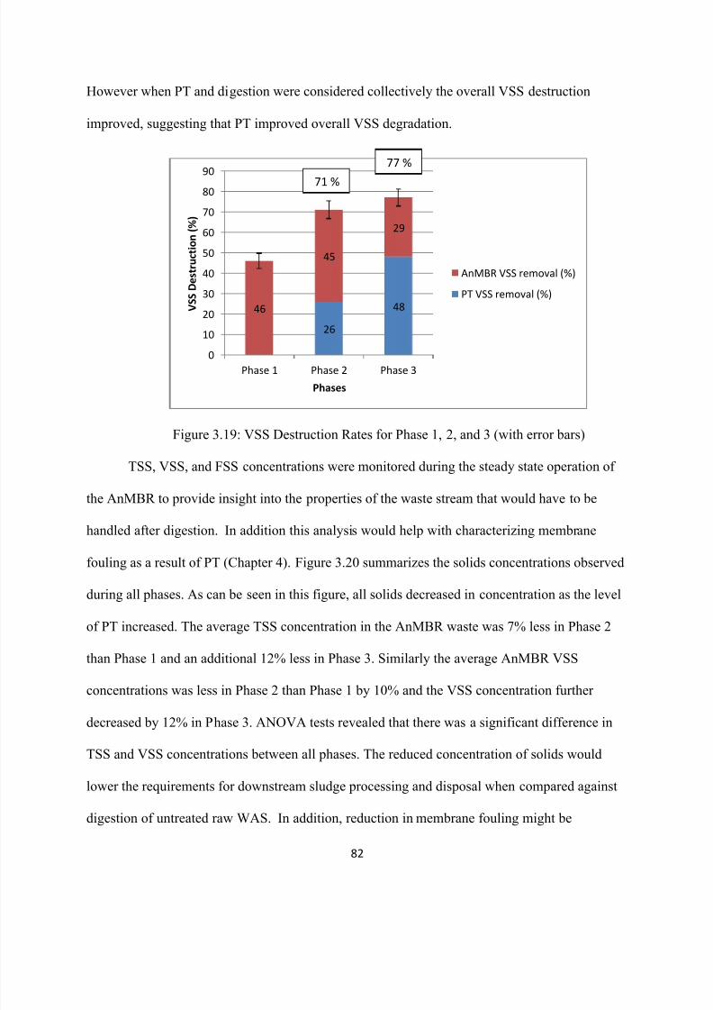
8/10/2019 Joshi Priyanka
http://slidepdf.com/reader/full/joshi-priyanka 98/166
82
However when PT and digestion were considered collectively the overall VSS destruction
improved, suggesting that PT improved overall VSS degradation.
Figure 3.19: VSS Destruction Rates for Phase 1, 2, and 3 (with error bars)
TSS, VSS, and FSS concentrations were monitored during the steady state operation of
the AnMBR to provide insight into the properties of the waste stream that would have to be
handled after digestion. In addition this analysis would help with characterizing membrane
fouling as a result of PT (Chapter 4). Figure 3.20 summarizes the solids concentrations observed
during all phases. As can be seen in this figure, all solids decreased in concentration as the level
of PT increased. The average TSS concentration in the AnMBR waste was 7% less in Phase 2
than Phase 1 and an additional 12% less in Phase 3. Similarly the average AnMBR VSS
concentrations was less in Phase 2 than Phase 1 by 10% and the VSS concentration further
decreased by 12% in Phase 3. ANOVA tests revealed that there was a significant difference in
TSS and VSS concentrations between all phases. The reduced concentration of solids would
lower the requirements for downstream sludge processing and disposal when compared against
digestion of untreated raw WAS. In addition, reduction in membrane fouling might be
26
4846
45
29
0
10
20
30
40
50
60
70
8090
Phase 1 Phase 2 Phase 3
V S S D e s t r u c t i o n ( % )
Phases
AnMBR VSS removal (%)
PT VSS removal (%)
71 %
77 %
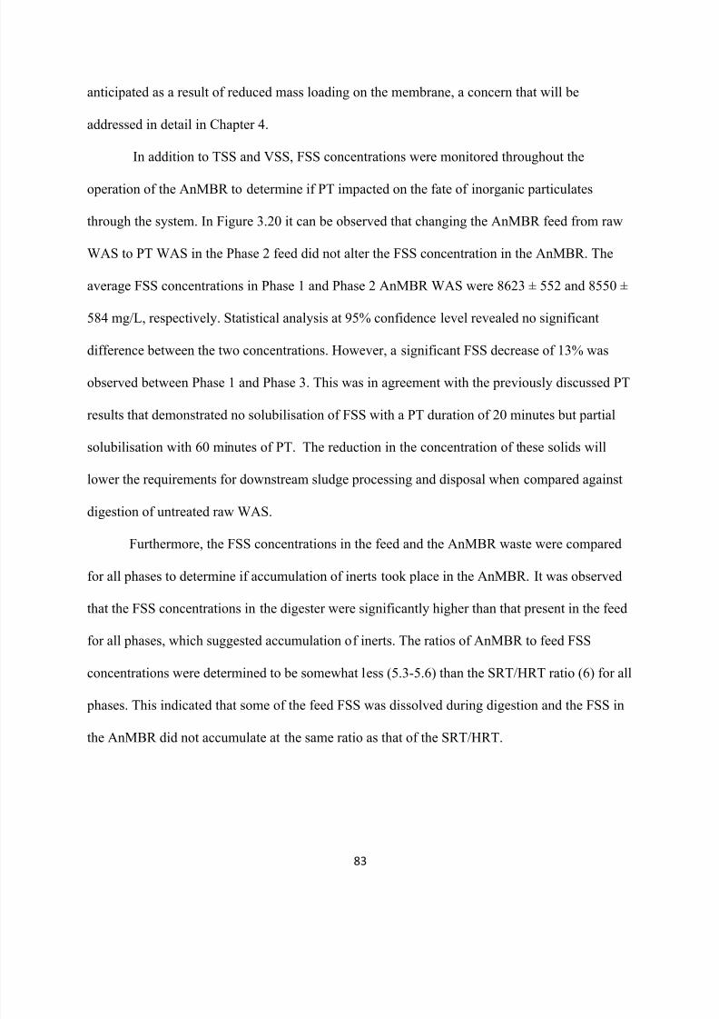
8/10/2019 Joshi Priyanka
http://slidepdf.com/reader/full/joshi-priyanka 99/166
83
anticipated as a result of reduced mass loading on the membrane, a concern that will be
addressed in detail in Chapter 4.
In addition to TSS and VSS, FSS concentrations were monitored throughout the
operation of the AnMBR to determine if PT impacted on the fate of inorganic particulates
through the system. In Figure 3.20 it can be observed that changing the AnMBR feed from raw
WAS to PT WAS in the Phase 2 feed did not alter the FSS concentration in the AnMBR. The
average FSS concentrations in Phase 1 and Phase 2 AnMBR WAS were 8623 ± 552 and 8550 ±
584 mg/L, respectively. Statistical analysis at 95% confidence level revealed no significant
difference between the two concentrations. However, a significant FSS decrease of 13% was
observed between Phase 1 and Phase 3. This was in agreement with the previously discussed PT
results that demonstrated no solubilisation of FSS with a PT duration of 20 minutes but partial
solubilisation with 60 minutes of PT. The reduction in the concentration of these solids will
lower the requirements for downstream sludge processing and disposal when compared against
digestion of untreated raw WAS.
Furthermore, the FSS concentrations in the feed and the AnMBR waste were compared
for all phases to determine if accumulation of inerts took place in the AnMBR. It was observed
that the FSS concentrations in the digester were significantly higher than that present in the feed
for all phases, which suggested accumulation of inerts. The ratios of AnMBR to feed FSS
concentrations were determined to be somewhat less (5.3-5.6) than the SRT/HRT ratio (6) for all
phases. This indicated that some of the feed FSS was dissolved during digestion and the FSS in
the AnMBR did not accumulate at the same ratio as that of the SRT/HRT.
8/10/2019 Joshi Priyanka
http://slidepdf.com/reader/full/joshi-priyanka 100/166
84
Figure 3.20: Average SS Concentrations in Phase 1, 2, and 3 AnMBR WAS (with error bars)
3.3.3.4. Organic Nitrogen Destruction and Analysis
Organic Nitrogen (ON) destruction can be employed as an alternative indication of the
performance of the AnMBR and thus was monitored throughout the AnMBR operation. Organic
nitrogen was calculated as the difference between TKN and Ammonia. For each phase, ON
destruction was calculated by comparing the cumulative mass of ON in the feed and outgoing
streams. Once the cumulative ON mass loadings in each stream was calculated, they were
graphed and the percent loss between the incoming and outgoing stream slopes yielded the ON
destruction rate. Figure 3.21 provides a sample ON destruction graph along with corresponding
calculations for Phase 1. From Figure 3.21 it can be seen that cumulative mass lines followed a
linear pattern and hence this demonstrates that steady state had been achieved during this
analysis. ON data for all other phases can be found in Appendix A8.
24658
16036
8623
22975
14425
8550
20183
12666
7518
0 4000 8000 12000 16000 20000 24000 28000
TSS
VSS
FSS
mg Solids/L
P a r a m e t e r s
Phase 3
Phase 2
Phase 1
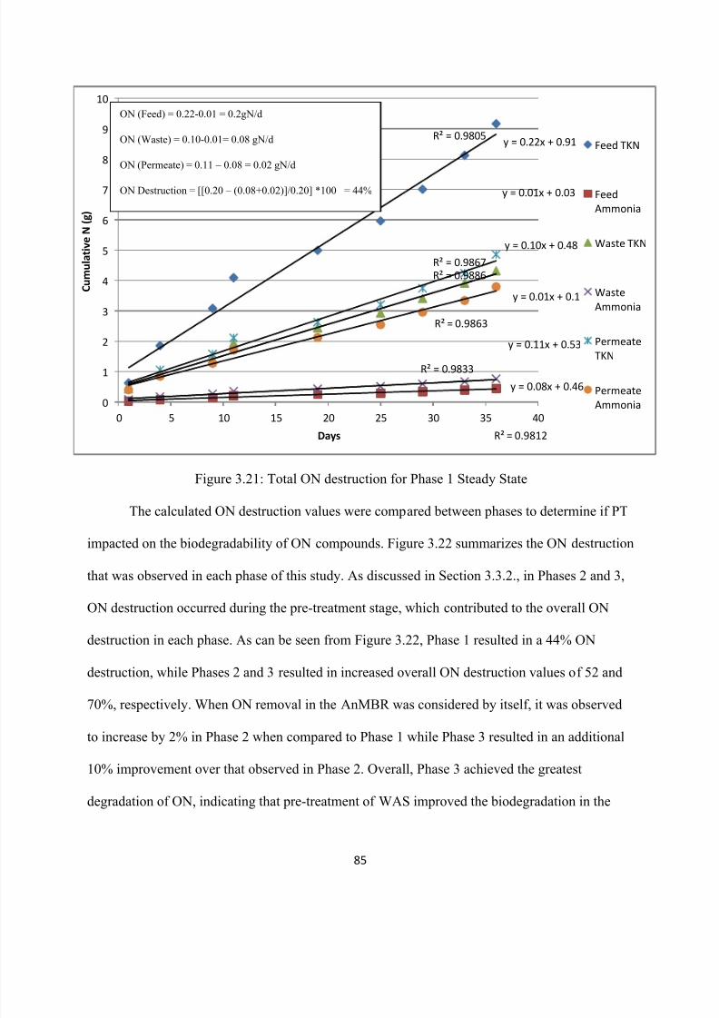
8/10/2019 Joshi Priyanka
http://slidepdf.com/reader/full/joshi-priyanka 101/166
85
y = 0.22x + 0.91R² = 0.9805
y = 0.01x + 0.03
R² = 0.9812
y = 0.10x + 0.48
R² = 0.9886
y = 0.01x + 0.1
R² = 0.9833
y = 0.11x + 0.53
R² = 0.9867
y = 0.08x + 0.46
R² = 0.9863
0
1
2
3
4
5
6
7
8
9
10
0 5 10 15 20 25 30 35 40
C u m u l a t i v e N ( g )
Days
Feed TKN
Feed
Ammonia
Waste TKN
Waste
Ammonia
Permeate
TKN
Permeate
Ammonia
Figure 3.21: Total ON destruction for Phase 1 Steady State
The calculated ON destruction values were compared between phases to determine if PT
impacted on the biodegradability of ON compounds. Figure 3.22 summarizes the ON destruction
that was observed in each phase of this study. As discussed in Section 3.3.2., in Phases 2 and 3,
ON destruction occurred during the pre-treatment stage, which contributed to the overall ON
destruction in each phase. As can be seen from Figure 3.22, Phase 1 resulted in a 44% ON
destruction, while Phases 2 and 3 resulted in increased overall ON destruction values of 52 and
70%, respectively. When ON removal in the AnMBR was considered by itself, it was observed
to increase by 2% in Phase 2 when compared to Phase 1 while Phase 3 resulted in an additional
10% improvement over that observed in Phase 2. Overall, Phase 3 achieved the greatest
degradation of ON, indicating that pre-treatment of WAS improved the biodegradation in the
ON (Feed) = 0.22-0.01 = 0.2gN/d
ON (Waste) = 0.10-0.01= 0.08 gN/d
ON (Permeate) = 0.11 – 0.08 = 0.02 gN/d
ON Destruction = [[0.20 – (0.08+0.02)]/0.20] *100 = 44%
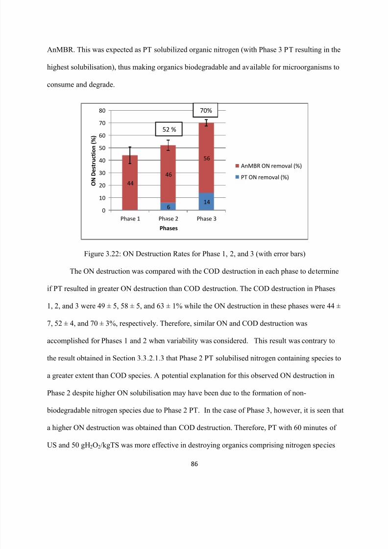
8/10/2019 Joshi Priyanka
http://slidepdf.com/reader/full/joshi-priyanka 102/166
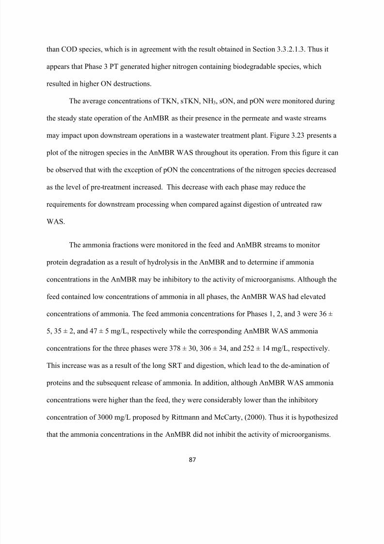
8/10/2019 Joshi Priyanka
http://slidepdf.com/reader/full/joshi-priyanka 103/166
87
than COD species, which is in agreement with the result obtained in Section 3.3.2.1.3. Thus it
appears that Phase 3 PT generated higher nitrogen containing biodegradable species, which
resulted in higher ON destructions.
The average concentrations of TKN, sTKN, NH3, sON, and pON were monitored during
the steady state operation of the AnMBR as their presence in the permeate and waste streams
may impact upon downstream operations in a wastewater treatment plant. Figure 3.23 presents a
plot of the nitrogen species in the AnMBR WAS throughout its operation. From this figure it can
be observed that with the exception of pON the concentrations of the nitrogen species decreased
as the level of pre-treatment increased. This decrease with each phase may reduce the
requirements for downstream processing when compared against digestion of untreated raw
WAS.
The ammonia fractions were monitored in the feed and AnMBR streams to monitor
protein degradation as a result of hydrolysis in the AnMBR and to determine if ammonia
concentrations in the AnMBR may be inhibitory to the activity of microorganisms. Although the
feed contained low concentrations of ammonia in all phases, the AnMBR WAS had elevated
concentrations of ammonia. The feed ammonia concentrations for Phases 1, 2, and 3 were 36 ±
5, 35 ± 2, and 47 ± 5 mg/L, respectively while the corresponding AnMBR WAS ammonia
concentrations for the three phases were 378 ± 30, 306 ± 34, and 252 ± 14 mg/L, respectively.
This increase was as a result of the long SRT and digestion, which lead to the de-amination of
proteins and the subsequent release of ammonia. In addition, although AnMBR WAS ammonia
concentrations were higher than the feed, they were considerably lower than the inhibitory
concentration of 3000 mg/L proposed by Rittmann and McCarty, (2000). Thus it is hypothesized
that the ammonia concentrations in the AnMBR did not inhibit the activity of microorganisms.
8/10/2019 Joshi Priyanka
http://slidepdf.com/reader/full/joshi-priyanka 104/166
88
Also observed from this discussion is that the PT phases had lower ammonia concentrations than
the control reactor. This observation will be discussed in the upcoming paragraphs.
Figure 3.23: Average Nitrogen Concentrations in Phase 1, 2, and 3 AnMBR WAS (with error
bars)
A cumulative mass balance was conducted on TKN in all three phases to monitor the
conservation of nitrogen species in this study. Figure 3.24 presents a cumulative mass balance of
TKN observed throughout this study. As can be seen from the figure, TKN masses remained
essentially constant in Phase 1 feed and AnMBR (waste and permeate streams). The cumulative
mass of TKN in the Phase 1 feed was 20.3 g N while the cumulative mass of TKN in the Phase 1
AnMBR (waste and permeate streams) was 19.5 gN. The small difference of 4% between the
Phase 1 TKN masses demonstrated that there was no significant lack of mass balance closure,
and thus was indicate of good data quality. In Phase 2 and Phase 3 differences of 12% and 18%
respectively were observed between the feed and AnMBR (permeate and waste streams) masses .
These differences were significantly different than the Phase 1 difference and thus there was a
lack of mass balance closure in Phases 2 and 3.
2132
815
378
437
1317
1654
613
306
307
1041
1560
398
252
145
1162
0 500 1000 1500 2000 2500
TKN
sTKN
Ammonia
sON
pON
mgN/L
Phase 3
Phase 2
Phase 1
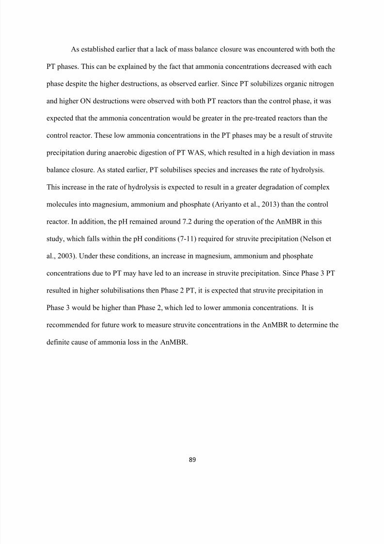
8/10/2019 Joshi Priyanka
http://slidepdf.com/reader/full/joshi-priyanka 105/166
89
As established earlier that a lack of mass balance closure was encountered with both the
PT phases. This can be explained by the fact that ammonia concentrations decreased with each
phase despite the higher destructions, as observed earlier. Since PT solubilizes organic nitrogen
and higher ON destructions were observed with both PT reactors than the control phase, it was
expected that the ammonia concentration would be greater in the pre-treated reactors than the
control reactor. These low ammonia concentrations in the PT phases may be a result of struvite
precipitation during anaerobic digestion of PT WAS, which resulted in a high deviation in mass
balance closure. As stated earlier, PT solubilises species and increases the rate of hydrolysis.
This increase in the rate of hydrolysis is expected to result in a greater degradation of complex
molecules into magnesium, ammonium and phosphate (Ariyanto et al., 2013) than the control
reactor. In addition, the pH remained around 7.2 during the operation of the AnMBR in this
study, which falls within the pH conditions (7-11) required for struvite precipitation (Nelson et
al., 2003). Under these conditions, an increase in magnesium, ammonium and phosphate
concentrations due to PT may have led to an increase in struvite precipitation. Since Phase 3 PT
resulted in higher solubilisations then Phase 2 PT, it is expected that struvite precipitation in
Phase 3 would be higher than Phase 2, which led to lower ammonia concentrations. It is
recommended for future work to measure struvite concentrations in the AnMBR to determine the
definite cause of ammonia loss in the AnMBR.
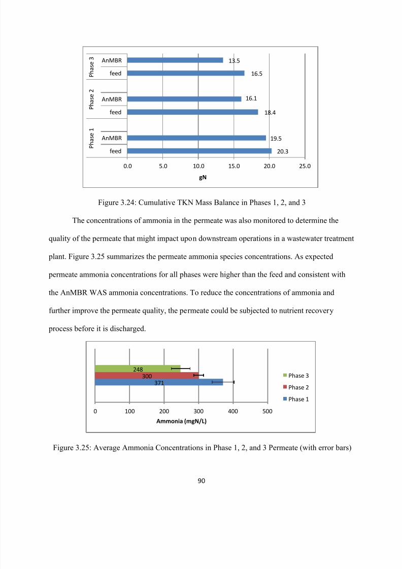
8/10/2019 Joshi Priyanka
http://slidepdf.com/reader/full/joshi-priyanka 106/166
90
Figure 3.24: Cumulative TKN Mass Balance in Phases 1, 2, and 3
The concentrations of ammonia in the permeate was also monitored to determine the
quality of the permeate that might impact upon downstream operations in a wastewater treatment
plant. Figure 3.25 summarizes the permeate ammonia species concentrations. As expected
permeate ammonia concentrations for all phases were higher than the feed and consistent with
the AnMBR WAS ammonia concentrations. To reduce the concentrations of ammonia and
further improve the permeate quality, the permeate could be subjected to nutrient recovery
process before it is discharged.
Figure 3.25: Average Ammonia Concentrations in Phase 1, 2, and 3 Permeate (with error bars)
20.3
19.5
18.4
16.1
16.5
13.5
0.0 5.0 10.0 15.0 20.0 25.0
feed
AnMBR
feed
AnMBR
feed
AnMBR
P h a s e 1
P h a s e 2
P h a s e 3
gN
371300
248
0 100 200 300 400 500
Ammonia (mgN/L)
Phase 3
Phase 2
Phase 1
8/10/2019 Joshi Priyanka
http://slidepdf.com/reader/full/joshi-priyanka 107/166
91
3.3.3.5. COD Decay Tests – Estimation of Biodegradable COD
COD decays tests were performed to determine the impact of pre-treatment on the
readily biodegradable fraction of COD in the WAS. It was hypothesized that PT would increase
the readily biodegradable fraction and that this fraction could be quantified by monitoring COD
removal during the period between feed cycles. These tests were performed for Phases 2 and 3,
once both phases had reached steady state. These tests were duplicated for both phases and the
procedure outlined below was followed.
In these tests, the concentrations of TCOD and SCOD in the system (AnMBR +
permeate holding tank) were measured every 5 hours by withdrawing 37.5 mL of AnMBR WAS.
To avoid complications with permeate withdrawal, the COD of the permeate was estimated by
measuring the SCOD of the AnMBR. The mass of TCOD and SCOD in the system was then
calculated by multiplying the volumes in the reactor and the permeate holding tank by their
respective COD concentrations at each sampling time. In order to determine the volume of
sludge remaining in the reactor, the volume of permeate collected at every withdrawal period
was subtracted from the working volume of the reactor. The masses of COD in the reactor and
the permeate holding tank were then added to determine the mass of COD in the system, which
was then plotted against time to produce a mass decay plot.
The COD decay plots for both phases are summarized in Figure 3.26 to compare the
COD consumption in the two PT phases. As mentioned earlier, this test was duplicated for each
phase and the error bars represent the variation between the duplicated tests. Each plot
corresponded to one reaction cycle, which was 24 hours for this study. As can be seen from the
figure, the highest COD concentration in the system was observed at the beginning of each cycle,
following WAS addition to the AnMBR. It can also be seen in the plot that the mass of COD in
8/10/2019 Joshi Priyanka
http://slidepdf.com/reader/full/joshi-priyanka 108/166
92
the system became effectively constant at the end of each reaction period (except for t=10 hours
in Phase 2), thus demonstrating that the biodegradable COD had been consumed by the end of
the cycle. The mass of COD in the system at t =10 hours in Phase 2 was lower than expected and
may have been a result of analytical error, thus resulting in a deviation from the true mass of
COD in the reactor at that time. Therefore, an estimated decay curve was generated for Phase 2
(Figure 3.26).
To compare the change in biodegradability between the two phases, the difference
between the mass of COD in reactor at the beginning and the end of the cycle in each phase was
assessed using Equation 3.3.
The average COD changes for Phase 2 and Phase 3 were 18 ± 1.3 % and 24 ± 0.1%,
respectively. A t-test at 95% confidence interval revealed that the extent of COD reduction was
significant different between the two phases. Therefore, PT in Phase 3 increased the fraction of
COD that could be degraded in the AnMBR as compared to Phase 2. The results from these tests
were thus in agreement with the COD destruction results in the previous section.
The rate of COD decline in the reactor was also monitored to estimate the amount of
readily biodegradable in both PT phases. As can be seen from Figure 3.26, the mass of COD in
the reactor declined more rapidly with Phase 3 compared to the Phase 2 pre-treated feed. In
Phase 2 the mass of COD declined from 85 to 70 gCOD after 10 hours of digestion, after which
the mass of COD in the system remained constant. By contrast In Phase 3 the mass of COD was
reduced from 81 to 61 g COD in 5 hours, after which the mass of COD in the system remained
constant. Hence, the results indicate that the Phase 3 pre-treated feed had a greater readily
biodegradable COD content than the Phase 2 pre-treated feed. Therefore PT of WAS with a
Eq. 3.3
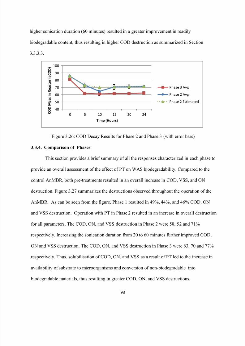
8/10/2019 Joshi Priyanka
http://slidepdf.com/reader/full/joshi-priyanka 109/166
93
higher sonication duration (60 minutes) resulted in a greater improvement in readily
biodegradable content, thus resulting in higher COD destruction as summarized in Section
3.3.3.3.
Figure 3.26: COD Decay Results for Phase 2 and Phase 3 (with error bars)
3.3.4. Comparison of Phases
This section provides a brief summary of all the responses characterized in each phase to
provide an overall assessment of the effect of PT on WAS biodegradability. Compared to the
control AnMBR, both pre-treatments resulted in an overall increase in COD, VSS, and ON
destruction. Figure 3.27 summarizes the destructions observed throughout the operation of the
AnMBR. As can be seen from the figure, Phase 1 resulted in 49%, 44%, and 46% COD, ON
and VSS destruction. Operation with PT in Phase 2 resulted in an increase in overall destruction
for all parameters. The COD, ON, and VSS destruction in Phase 2 were 58, 52 and 71%
respectively. Increasing the sonication duration from 20 to 60 minutes further improved COD,
ON and VSS destruction. The COD, ON, and VSS destruction in Phase 3 were 63, 70 and 77%
respectively. Thus, solubilisation of COD, ON, and VSS as a result of PT led to the increase in
availability of substrate to microorganisms and conversion of non-biodegradable into
biodegradable materials, thus resulting in greater COD, ON, and VSS destructions.
40
50
60
70
80
90
100
0 5 10 15 20 24 C O D M a s s i n R e a c t o r ( g C O D )
Time (Hours)
Phase 3 Avg
Phase 2 Avg
Phase 2 Estimated
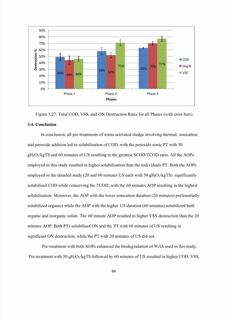
8/10/2019 Joshi Priyanka
http://slidepdf.com/reader/full/joshi-priyanka 110/166
94
Figure 3.27: Total COD, VSS, and ON Destruction Rates for all Phases (with error bars)
3.4. Conclusion
In conclusion, all pre-treatments of waste activated sludge involving thermal, sonication
and peroxide addition led to solubilisation of COD, with the peroxide-sonic PT with 50
gH2O2/kgTS and 60 minutes of US resulting in the greatest SCOD/TCOD ratio. All the AOPs
employed in this study resulted in higher solubilisation than the individuals PT. Both the AOPs
employed in the detailed study (20 and 60 minutes US each with 50 gH2O2/kgTS) significantly
solubilised COD while conserving the TCOD, with the 60 minutes AOP resulting in the highest
solubilisation. Moreover, the AOP with the lower sonication duration (20 minutes) preferentially
solubilized organics while the AOP with the higher US duration (60 minutes) solubilized both
organic and inorganic solids. The 60 minute AOP resulted in higher VSS destruction than the 20
minutes AOP. Both PTs solubilised ON and the PT with 60 minutes of US resulting in
significant ON destruction, while the PT with 20 minutes of US did not.
Pre-treatment with both AOPs enhanced the biodegradation of WAS used in this study.
Pre-treatment with 50 gH2O2/kgTS followed by 60 minutes of US resulted in higher COD, VSS,
49%58% 63%
44%52%
70%
46%
71%77%
0%
10%
20%
30%
40%
50%
60%
70%
80%
90%
Phase 1 Phase 2 Phase 3
D e s t r u c t i o
n %
Phases
COD
Org N
VSS
8/10/2019 Joshi Priyanka
http://slidepdf.com/reader/full/joshi-priyanka 111/166
95
and ON destructions than pre-treatment with 50 gH2O2/kgTS followed by 20 minutes of US.
This was attributed to solubilisation and an increase in the biodegradable fraction in the Phase 3
PT. Some accumulation of colloids and inerts was observed in the AnMBR reactor. PT resulted
in a reduction in the mass flow of solids and organics. Thus a PT-AnMBR system may reduce
the requirements for downstream processing when compared with digestion of untreated raw
WAS.
8/10/2019 Joshi Priyanka
http://slidepdf.com/reader/full/joshi-priyanka 112/166
96
Chapter 4: Membrane Performance of AnMBR treating Raw and Pre-treated WAS
4.1. Introduction
Anaerobic digestion (AD) is a common sludge stabilization method employed in
wastewater treatment plants that not only converts the organic matter into a renewable source of
energy i.e. biogas, but also decreases the amount of solids while destroying a majority of the
pathogens in the sludge (Abelleira et al., 2012). However conventional anaerobic processes
typically need to be operated at long hydraulic residence times and require large bioreactor
volumes to accommodate the rate limiting hydrolysis process and the slow growth rates of
methanogens (Bougrier et al., 2006). The incorporation of membranes into the design of
anaerobic digesters has the potential to considerably reduce bioreactor volumes by decoupling
the HRT from the SRT (Dagnew, 2010). The operation of the bioreactors at relatively shorter
HRTs and longer SRTs can reduce the bioreactor volume, while accomplishing higher organic
loading and destruction rates.
Although AnMBRs appear to provide considerable advantages over conventional
digesters when bioreactor performance is considered, a potential challenge is the fouling of
membranes due to the accumulation of microorganisms, colloids, solutes, and cell debris in or on
membrane surfaces (Meng el al., 2009). Membrane fouling results in an increased filtration
resistance, thus reducing the permeate flux (Judd, 2008) or conversely, the TMP increases if
operated in constant flux mode. The inefficient operation of membranes due to fouling will
require elevated maintenance and energy costs and may require frequent replacement of
membranes, which in turn increases costs. Therefore, characterization of fouling is desirable as it
will facilitate the development of strategies that might be employed to reduce these costs.
8/10/2019 Joshi Priyanka
http://slidepdf.com/reader/full/joshi-priyanka 113/166
97
The potential for membrane fouling is elevated when treating high solids waste streams
such as WAS. In this application, the high solids concentrations of the feed stream, and the
amplification of non-biodegradable suspended solids concentrations in the MLSS due to the ratio
of SRT/HRT can lead to high MLSS concentrations that may lead to membrane fouling. The
MLSS concentrations may be reduced through the use of sludge pretreatment (PT) technologies.
PT technologies are growing in popularity as they promise to increase WAS biodegradability.
However, PT has been shown to produce colloidal solids that may accumulate in AnMBRs if
they are not biodegraded. The presence of colloids has been identified as a significant factor in
membrane fouling when treating sludge (Wu et al., 2009 and Fan et al., 2006). Operation at
extended SRTs has also been found to result in colloid generation due to hydrolysis of
particulates. Hence, operation at long SRTs in combination with pre-treatment (PT) may lead to
a higher concentration of colloids than untreated WAS due to the solubilising effect of PT.
There is however little evidence in the literature to indicate whether the increase in colloid
concentrations with PT would offset the benefits that might be achieved with lower MLSS.
While PT may reduce fouling when digesting WAS it is prudent to ensure that membrane
flux is maximized through implementation of strategies that are known to minimize fouling. A
number of strategies to minimize and control fouling have been reported in prior studies. For
instance, operating the membrane below the critical flux has been reported to result in minimal
fouling (Jeison and van Lier, 2006a). Another method to control fouling is to integrate a period
of relaxation into the membrane operation rather than operating with continuous permeation
(Jude, 2006). For instance, Dagnew et al., (2012) compared the performance of a tubular
membrane with continuous permeation at a flux of 30 litres per m2 per hour (LMH) with that of a
membrane operating on a cycle with 5 minutes of permeation followed by 1 minute of relaxation.
8/10/2019 Joshi Priyanka
http://slidepdf.com/reader/full/joshi-priyanka 114/166
98
They observed that relaxation extended the operation of the membrane by limiting the maximum
transmembrane pressure (TMP) to 30 kilopascals (kPa) while continuous operation led to a TMP
of 80 kPa, thus demonstrating increased fouling of the membrane.
In addition to a relaxed mode of operation and operation below critical flux, regular
maintenance cleaning can also ensure reduced fouling and long term operation of membranes
despite high solids concentrations and operating flux. For instance, Pierkiel and Lanting, (2005)
attributed the long term successful performance of an AnMBR treating a combination of PS and
WAS with an MLSS of 5-20 g/L and flux of 146 and 66.7-83 LMH to daily and monthly
maintenance cleaning with a combination of phosphoric acid and sodium hydroxide. In addition
to a phosphoric acid and sodium hydroxide combination, a variety of chemical agents have been
successfully used to perform maintenance cleaning of membranes. For instance, Lee et al.,
(2001) achieved a flux recovery of up to 86% of the initial membrane flux for an AnMBR
treating swine manure by subjecting the membrane to a cleaning by an alkaline solution followed
by an acidic agent. In another study, Kang et al., (2002) observed that the permeate flux
increased by two times after performing acidic cleaning. The cleaning efficiency has also been
observed to be dependent on the sequence of cleaning. For instance, Dagnew, (2010) observed
that cleaning with NaOH followed by citric acid caused further fouling of the membrane due to
the precipitation of inorganic materials that were present on the cake layer as a result of the
increase in pH. However when the cleaning order was reversed, almost 100% of the flux was
recovered. Therefore, in addition to regular maintenance cleaning, it is essential to determine the
ideal cleaning sequence when using a combination of chemicals to maintain membrane
performance.
8/10/2019 Joshi Priyanka
http://slidepdf.com/reader/full/joshi-priyanka 115/166
99
Operation with high MLSS concentration does not necessarily translate to a need for
frequent cleaning. In some cases, membrane performance can be maintained by applying gas
sparging or cross flow velocities to scour foulants that are deposited on or in the membrane. For
instance, Padmasiri et al., (2007) operated a side stream AnMBR with MLSS concentrations of
27 and 49 g/L to treat swine manure with no cleaning employed during its operation. The long
term performance of the membrane was attributed to the use of high cross-flow velocities that
prevented deposition of foulants on or in the membrane. However, a decline in the biological
activity of the micro-organisms was also reported, which may be attributed to an interruption of
the syntrophic interaction of acetogenic and methanogenic organisms as a result of high
velocities (Brockmann and Seyfried, 1997 and Hernandez et al., 2002). Hence strategies to
minimize the decline in flux without excessive shear rates need to be explored.
In conclusion, relatively few studies have evaluated membrane fouling in the digestion of
high solids streams in AnMBRs. In addition, there is little information available on the impact of
an integrated PT-AnMBR system on membrane fouling. This study aimed to determine the
feasibility of anaerobic digestion of WAS that was pre-treated with a peroxide+sonic AOP in an
AnMBR. In order to determine if such a system can be successfully applied, this study monitored
the effect of changing biomass characteristics due to PT on membrane fouling and critical flux.
In addition, this study examined if operation of a hollow fibre membrane with a fouling
minimizing strategy that involved maintenance cleaning, gas sparging, a relaxed mode of
operation, and an operational flux below the critical flux is feasible.
8/10/2019 Joshi Priyanka
http://slidepdf.com/reader/full/joshi-priyanka 116/166
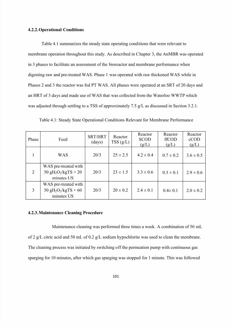
8/10/2019 Joshi Priyanka
http://slidepdf.com/reader/full/joshi-priyanka 117/166
101
4.2.2. Operational Conditions
Table 4.1 summarizes the steady state operating conditions that were relevant to
membrane operation throughout this study. As described in Chapter 3, the AnMBR was operated
in 3 phases to facilitate an assessment of the bioreactor and membrane performance when
digesting raw and pre-treated WAS. Phase 1 was operated with raw thickened WAS while in
Phases 2 and 3 the reactor was fed PT WAS. All phases were operated at an SRT of 20 days and
an HRT of 3 days and made use of WAS that was collected from the Waterloo WWTP which
was adjusted through settling to a TSS of approximately 7.5 g/L as discussed in Section 3.2.1.
Table 4.1: Steady State Operational Conditions Relevant for Membrane Performance
Phase FeedSRT/HRT
(days)
Reactor
TSS (g/L)
ReactorSCOD
(g/L)
ReactorffCOD
(g/L)
ReactorcCOD
(g/L)
1 WAS 20/3 25 ± 2.5 4.2 ± 0.4 0.7 ± 0.2 3.6 ± 0.5
2
WAS pre-treated with
50 gH2O2/kgTS + 20minutes US
20/3 23 ± 1.5 3.3 ± 0.6 0.3 ± 0.1 2.9 ± 0.6
3
WAS pre-treated with
50 gH2O2/kgTS + 60
minutes US
20/3 20 ± 0.2 2.4 ± 0.1 0.4± 0.1 2.0 ± 0.2
4.2.3. Maintenance Cleaning Procedure
Maintenance cleaning was performed three times a week. A combination of 50 mL
of 2 g/L citric acid and 50 mL of 0.2 g/L sodium hypochlorite was used to clean the membrane.
The cleaning process was initiated by switching off the permeation pump with continuous gas
sparging for 10 minutes, after which gas sparging was stopped for 1 minute. This was followed
8/10/2019 Joshi Priyanka
http://slidepdf.com/reader/full/joshi-priyanka 118/166
102
by backwashing with each chemical for 40 seconds of backpulse and 4 minutes of relaxation.
This cleaning cycle was repeated until 50 mL of each chemical was used. After backwashing, the
gas sparging pump was switched on for 5 minutes, after which regular permeation of the
membrane was commenced.
4.2.4. Critical Flux Determination
Critical flux tests were conducted using the method introduced by Field et al., (1995).
The critical flux test involved increasing the permeate flux in fixed increments for constant time
periods and monitoring the TMP at each flux. A plot of this data reveals a linear relation between
the TMP and flux within the sub-critical flux range and an exponential relation beyond the
critical flux range. The exponential increase in TMP indicates rapid accumulation of foulants.
Critical flux tests were conducted at steady state in Phase 2 and Phase 3. For each flux step, the
increment in flux was 6 LMH. The duration of each step was 10 min and this was followed by a
2 min relaxation time to prevent accumulation of foulants before the next flux value was
implemented. Critical flux tests were duplicated in each phase to determine if this test was
reproducible.
4.2.5. Sample Analysis
Sample analyses were performed according to the methods described in Section 3.2.6.
COD and solids analyses were conducted to characterize the biomass and determine its effect on
membrane fouling. All measurements were carried out in duplicate.
8/10/2019 Joshi Priyanka
http://slidepdf.com/reader/full/joshi-priyanka 119/166
103
4.3. Results
The following sections will discuss the impact of operating the bench scale AnMBR with
raw and PT WAS as a feed on the performance of the hollow fibre membrane. Apart from
monitoring the overall performance and fouling rate of the membrane throughout AnMBR
operation, this study examined trends between solids and colloidal concentrations and membrane
fouling. Lastly, the results of critical flux tests that were conducted to attain additional insight
into the potential operating flux under differing PT conditions will be assessed. Throughout these
analyses, the efficiency of the fouling minimizing strategy adopted for this study was monitored.
4.3.1. Overall Membrane Performance
As mentioned in Chapter 3, the AnMBR was manually fed with WAS once a day and was
then operated with continuous permeation for the remainder of the daily cycle. In this operation,
the volume of sludge in the reactor was at its highest level immediately after feeding and then
decreased until the daily permeate volume was collected. Since the TMP was affected by the
head pressure between the TMP gauge and the liquid level, this fluctuation in liquid level in the
reactor resulted in a daily fluctuation in TMP. Hence, two TMP patterns were observed in each
cycle; one when the liquid level in the reactor was descending (daily permeate volume of 1.275
L not collected) and the other when the daily permeate volume had already been collected. For
the purposes of this study, the TMP values for the period spanning from the beginning of the
daily AnMBR operation cycle until the daily permeate volume was collected will be referred to
as the low range TMPs, while the TMPs after the permeate volume has been collected will be
referred to as high range TMPs.
8/10/2019 Joshi Priyanka
http://slidepdf.com/reader/full/joshi-priyanka 120/166
104
The high and low range TMPs were monitored to obtain insight into membrane
performance over the range of feed compositions to the AnMBR. Figure 4.1 summarizes the
TMP observed throughout the operation of the AnMBR. From the figure it is seen that the
operation of the membrane was steady over the length of the study until the membrane was
replaced during Phase 2 operation. The membrane was replaced because the TMP rose to 60 kPa
after feeding the reactor for 2 consecutive days. The increase in TMP was later found to be due
to a fault in the head of the gas sparging pump, which led to a decline in the sparging rate. This
result was consistent with that of Padmasiri et al., (2007), where the long term performance of
the membrane was attributed to the use of high cross-flow velocities that prevented deposition of
foulants on or in the membrane. Therefore, an effective sparging rate was required to minimize
membrane fouling and maintain the performance of the membrane.
The TMP values that were recorded prior to and after membrane replacement were
compared to determine if any fouling had occurred before the replacement of the membrane. As
can be seen in Figure 4.1, both ranges of TMP reduced slightly after replacing the membrane.
The higher TMP range decreased from approximately 4.2 to 3.6 kPa and the lower TMP range
decreased from 3.3 to 3.2 kPa when the membrane was replaced (Day 140). This decrease
suggested that some fouling had occurred in Phase 1 and Phase 2 before the replacement of the
membrane.
The initial TMP observed with the second membrane was compared with the early Phase
1 TMP values to determine if both the membranes exhibited similar initial TMPs after start-up.
From Figure 4.1, it can be seen that the high range TMP after 1 month of start-up was low (3.6
kPa) and similar to the initial TMP of the second membrane (3.7 kPa). Since TMP was only
monitored from Day 30 of AnMBR operation, the behaviour of the first membrane during the
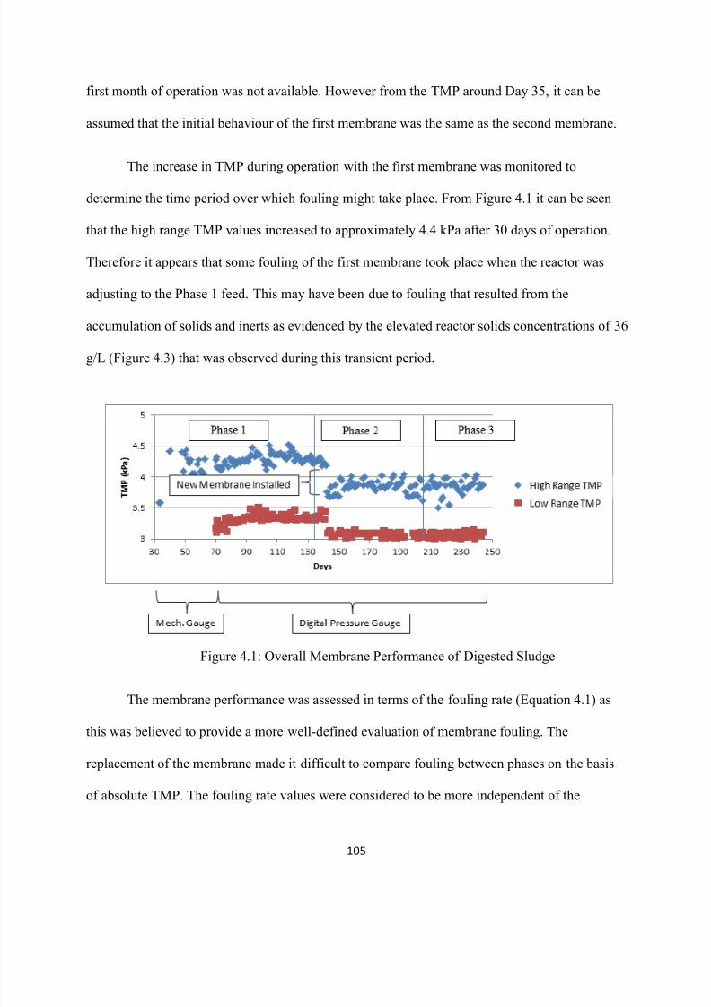
8/10/2019 Joshi Priyanka
http://slidepdf.com/reader/full/joshi-priyanka 121/166
105
first month of operation was not available. However from the TMP around Day 35, it can be
assumed that the initial behaviour of the first membrane was the same as the second membrane.
The increase in TMP during operation with the first membrane was monitored to
determine the time period over which fouling might take place. From Figure 4.1 it can be seen
that the high range TMP values increased to approximately 4.4 kPa after 30 days of operation.
Therefore it appears that some fouling of the first membrane took place when the reactor was
adjusting to the Phase 1 feed. This may have been due to fouling that resulted from the
accumulation of solids and inerts as evidenced by the elevated reactor solids concentrations of 36
g/L (Figure 4.3) that was observed during this transient period.
Figure 4.1: Overall Membrane Performance of Digested Sludge
The membrane performance was assessed in terms of the fouling rate (Equation 4.1) as
this was believed to provide a more well-defined evaluation of membrane fouling. The
replacement of the membrane made it difficult to compare fouling between phases on the basis
of absolute TMP. The fouling rate values were considered to be more independent of the
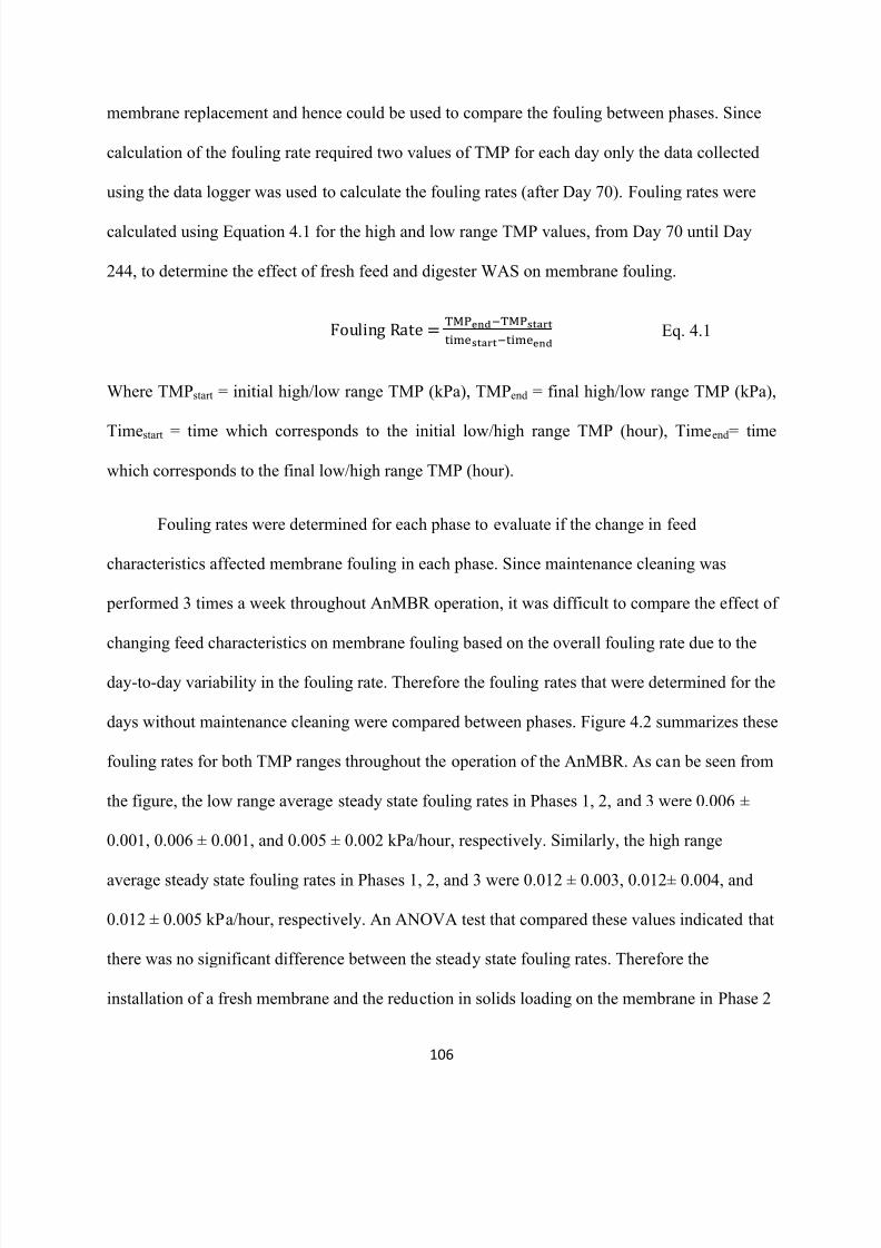
8/10/2019 Joshi Priyanka
http://slidepdf.com/reader/full/joshi-priyanka 122/166
106
membrane replacement and hence could be used to compare the fouling between phases. Since
calculation of the fouling rate required two values of TMP for each day only the data collected
using the data logger was used to calculate the fouling rates (after Day 70). Fouling rates were
calculated using Equation 4.1 for the high and low range TMP values, from Day 70 until Day
244, to determine the effect of fresh feed and digester WAS on membrane fouling.
Where TMPstart = initial high/low range TMP (kPa), TMPend = final high/low range TMP (kPa),
Timestart = time which corresponds to the initial low/high range TMP (hour), Time end= time
which corresponds to the final low/high range TMP (hour).
Fouling rates were determined for each phase to evaluate if the change in feed
characteristics affected membrane fouling in each phase. Since maintenance cleaning was
performed 3 times a week throughout AnMBR operation, it was difficult to compare the effect of
changing feed characteristics on membrane fouling based on the overall fouling rate due to the
day-to-day variability in the fouling rate. Therefore the fouling rates that were determined for the
days without maintenance cleaning were compared between phases. Figure 4.2 summarizes these
fouling rates for both TMP ranges throughout the operation of the AnMBR. As can be seen from
the figure, the low range average steady state fouling rates in Phases 1, 2, and 3 were 0.006 ±
0.001, 0.006 ± 0.001, and 0.005 ± 0.002 kPa/hour, respectively. Similarly, the high range
average steady state fouling rates in Phases 1, 2, and 3 were 0.012 ± 0.003, 0.012± 0.004, and
0.012 ± 0.005 kPa/hour, respectively. An ANOVA test that compared these values indicated that
there was no significant difference between the steady state fouling rates. Therefore the
installation of a fresh membrane and the reduction in solids loading on the membrane in Phase 2
Eq. 4.1
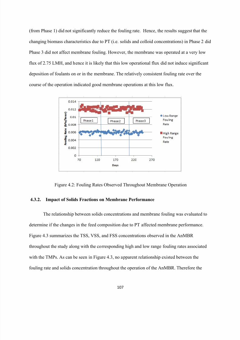
8/10/2019 Joshi Priyanka
http://slidepdf.com/reader/full/joshi-priyanka 123/166
107
(from Phase 1) did not significantly reduce the fouling rate. Hence, the results suggest that the
changing biomass characteristics due to PT (i.e. solids and colloid concentrations) in Phase 2 did
Phase 3 did not affect membrane fouling. However, the membrane was operated at a very low
flux of 2.75 LMH, and hence it is likely that this low operational flux did not induce significant
deposition of foulants on or in the membrane. The relatively consistent fouling rate over the
course of the operation indicated good membrane operations at this low flux.
Figure 4.2: Fouling Rates Observed Throughout Membrane Operation
4.3.2. Impact of Solids Fractions on Membrane Performance
The relationship between solids concentrations and membrane fouling was evaluated to
determine if the changes in the feed composition due to PT affected membrane performance.
Figure 4.3 summarizes the TSS, VSS, and FSS concentrations observed in the AnMBR
throughout the study along with the corresponding high and low range fouling rates associated
with the TMPs. As can be seen in Figure 4.3, no apparent relationship existed between the
fouling rate and solids concentration throughout the operation of the AnMBR. Therefore the
8/10/2019 Joshi Priyanka
http://slidepdf.com/reader/full/joshi-priyanka 124/166
108
decrease in solids loading on the membrane did not result in any significant reduction in
membrane fouling. In addition, accumulation of inerts in all three phases (Chapter 3) did not
significantly affect the fouling rate. Overall there appeared to be little relationship between these
solids concentration and membrane fouling. This may have been due to the combination of the
high cleaning frequency of 3 times a week, the high gas sparging rate of 2 L/min, the low
operational flux of 2.75 LMH and a relaxed permeation cycle. Therefore, the operational design
was successful in minimizing the likelihood of excessive fouling despite high solids
concentrations.
Figure 4.3: Effect of Solids Loading on Membrane Fouling
4.3.3. Impact of COD Fractions on Membrane Performance
The impact of colloid concentrations on membrane performance was assessed since
colloids have been identified as a significant foulant in AnMBRs in other studies (Wu et al.,
2009 and Fan et al., 2006). For this study, colloidal COD (cCOD) was determined as the
difference between the SCOD and ffCOD filtrate values. Figure 4.4 summarizes the average
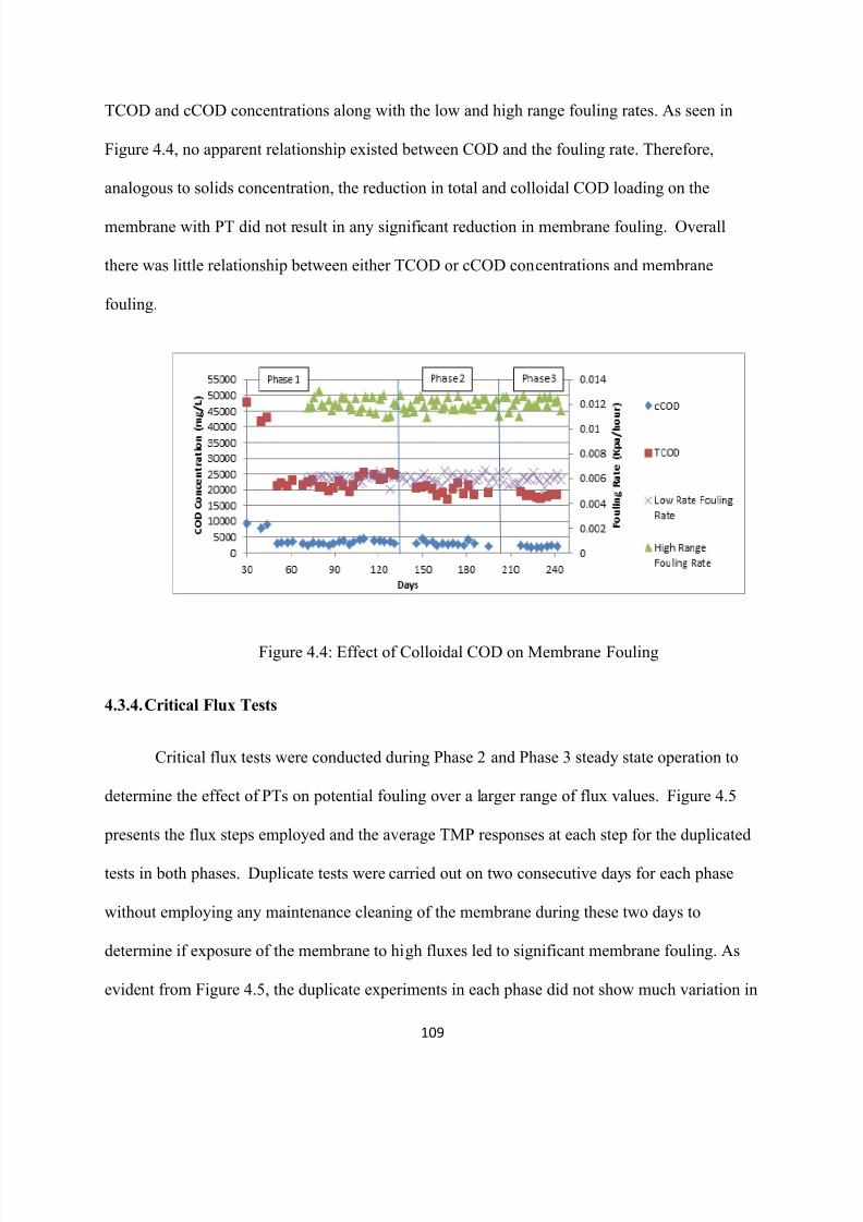
8/10/2019 Joshi Priyanka
http://slidepdf.com/reader/full/joshi-priyanka 125/166
109
TCOD and cCOD concentrations along with the low and high range fouling rates. As seen in
Figure 4.4, no apparent relationship existed between COD and the fouling rate. Therefore,
analogous to solids concentration, the reduction in total and colloidal COD loading on the
membrane with PT did not result in any significant reduction in membrane fouling. Overall
there was little relationship between either TCOD or cCOD concentrations and membrane
fouling.
Figure 4.4: Effect of Colloidal COD on Membrane Fouling
4.3.4. Critical Flux Tests
Critical flux tests were conducted during Phase 2 and Phase 3 steady state operation to
determine the effect of PTs on potential fouling over a larger range of flux values. Figure 4.5
presents the flux steps employed and the average TMP responses at each step for the duplicated
tests in both phases. Duplicate tests were carried out on two consecutive days for each phase
without employing any maintenance cleaning of the membrane during these two days to
determine if exposure of the membrane to high fluxes led to significant membrane fouling. As
evident from Figure 4.5, the duplicate experiments in each phase did not show much variation in
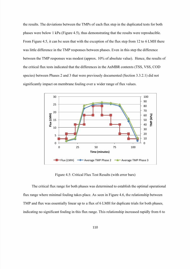
8/10/2019 Joshi Priyanka
http://slidepdf.com/reader/full/joshi-priyanka 126/166
110
the results. The deviations between the TMPs of each flux step in the duplicated tests for both
phases were below 1 kPa (Figure 4.5), thus demonstrating that the results were reproducible.
From Figure 4.5, it can be seen that with the exception of the flux step from 12 to 6 LMH there
was little difference in the TMP responses between phases. Even in this step the difference
between the TMP responses was modest (approx. 10% of absolute value). Hence, the results of
the critical flux tests indicated that the differences in the AnMBR contents (TSS, VSS, COD
species) between Phases 2 and 3 that were previously documented (Section 3.3.2.1) did not
significantly impact on membrane fouling over a wider range of flux values.
Figure 4.5: Critical Flux Test Results (with error bars)
The critical flux range for both phases was determined to establish the optimal operational
flux range where minimal fouling takes place. As seen in Figure 4.6, the relationship between
TMP and flux was essentially linear up to a flux of 6 LMH for duplicate trials for both phases,
indicating no significant fouling in this flux range. This relationship increased rapidly from 6 to
0
10
20
30
40
50
60
70
80
90
100
0
5
10
15
20
25
30
0 25 50 75 100
T M P ( k P a )
F l u x ( L M H )
Time (minutes)
Flux (LMH) Average TMP Phase 2 Average TMP Phase 3
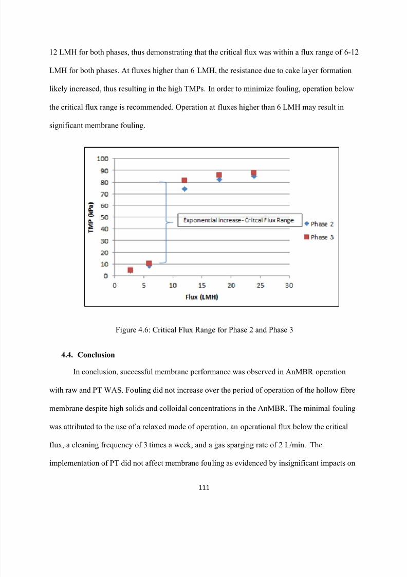
8/10/2019 Joshi Priyanka
http://slidepdf.com/reader/full/joshi-priyanka 127/166
111
12 LMH for both phases, thus demonstrating that the critical flux was within a flux range of 6-12
LMH for both phases. At fluxes higher than 6 LMH, the resistance due to cake layer formation
likely increased, thus resulting in the high TMPs. In order to minimize fouling, operation below
the critical flux range is recommended. Operation at fluxes higher than 6 LMH may result in
significant membrane fouling.
Figure 4.6: Critical Flux Range for Phase 2 and Phase 3
4.4. Conclusion
In conclusion, successful membrane performance was observed in AnMBR operation
with raw and PT WAS. Fouling did not increase over the period of operation of the hollow fibre
membrane despite high solids and colloidal concentrations in the AnMBR. The minimal fouling
was attributed to the use of a relaxed mode of operation, an operational flux below the critical
flux, a cleaning frequency of 3 times a week, and a gas sparging rate of 2 L/min. The
implementation of PT did not affect membrane fouling as evidenced by insignificant impacts on

8/10/2019 Joshi Priyanka
http://slidepdf.com/reader/full/joshi-priyanka 128/166
112
the fouling rates and through the critical flux tests. The critical flux range for Phase 2 and 3 was
determined to be 6 to 12 LMH and these values appeared to be independent of the biomass
concentrations in the AnMBR. Thus the results of this study demonstrate that a hollow fibre
membrane can be applied to filter anaerobically digested sludges that have undergone PT which
generates high concentrations of colloids and inerts.
8/10/2019 Joshi Priyanka
http://slidepdf.com/reader/full/joshi-priyanka 129/166
113
Chapter 5: Conclusions
This chapter provides a summary of significant conclusions related to this study. The
chapter commences with conclusions that were drawn from a comparison of thermal, sonication,
and peroxide-sonic PT that was based on COD analyses. This study compared thermal PT at 150
and 170°C for 30 minutes, sonication at 10 and 20 minutes and a peroxide-sonic AOP with
hydrogen peroxide doses of 5, 25, and 50 gH2O2/kgTS and US durations of 10, 20, 30, and 60
minutes. This section is followed by conclusions that were derived from a detailed study that
examined COD, nitrogen, and solids responses in PT and subsequent AnMBR digestion when
PTs that consisted of 50 gH2O2/kgTS followed by 20 minutes of US and 50 gH2O2/kgTS
followed by 60 minutes of US were examined. Finally, this chapter provides conclusions related
to membrane performance that were developed after observing operation during digestion of raw
and PT WAS with an AnMBR.
5.1. Comparison of Pre-treatments – Preliminary Tests
All PTs resulted in an increase in the solubilisation ratio, thus resulting in high colloidal
and soluble COD concentrations.
Pre-treatment with 50 gH2O2/kgTS and 60 minutes of US resulted in the highest fraction
of soluble COD of 46% and in an insignificant loss in TCOD (about 7%), implying no
loss in substrate for potential biogas production.
The 50 gH2O2/kgTS + 60 minutes US AOP and the other AOPs (with 20-30 minutes US
and 50 gH2O
2/kgTS) resulted in similar fractions of cCOD 25 and 21-24%, respectively.
However the ffCOD fraction of the 60 minute US AOP (22%) was higher than the other
AOPs (11-12%), thus implying that the 60 minutes US AOP was more effective in
solubilising particulates into soluble COD than the other AOPs.

8/10/2019 Joshi Priyanka
http://slidepdf.com/reader/full/joshi-priyanka 130/166
114
The results from this study demonstrated that a sonication + peroxide AOP resulted in
higher solubilisation than individual sonication PT.
In terms of the hydrogen peroxide and sonication AOP, sonication duration and the
interaction term (sonication + peroxide) were determined to have a greater impact on
sludge solubilisation than hydrogen peroxide dose. This was attributed to the low doses
of peroxide.
5.2. Comparison of the 20 and 60 minutes US AOP – Detailed Tests
In order to assess the effects of sonication duration on the physico-chemical properties
and biodegradability of WAS, two AOPs were selected from the preliminary tests for further
study – one with a low sonication duration of 20 minutes and another with a considerably higher
treatment time of 60 minutes, each with a peroxide dose of 50 gH2O2/kgTS.
5.2.1. Physico-chemical Comparison of the 20 and 60 minutes US AOP
Both pre-treatments resulted in minimal TCOD losses (of 4-6%) and substantially higher
ratios of SCOD/TCOD (33% for the 20 minutes AOP and 40% for the 60 minutes AOP),
and thus higher concentrations of truly soluble COD and colloids than the raw samples.
PT with 60 minutes of sonication resulted in higher ffCOD and cCOD fractions (16 and
24%) than the AOP with 20 minutes of sonication (12 and 21%).
The 60 minute AOP solubilised both VSS and FSS but the 20 minutes AOP solubilised
only VSS.
Both PTs resulted in VSS solids degradation, with the AOP with 60 minutes of US
duration resulting in a significantly higher VSS destruction (46%) than the AOP with 20
minutes of US (26%) as a result of high solubilisations.
8/10/2019 Joshi Priyanka
http://slidepdf.com/reader/full/joshi-priyanka 131/166
115
Both PTs resulted in ON solubilisation, with the AOP with 60 minutes of sonication
resulting in a higher solubilisation (47%). In addition, the AOP with 60 minutes
sonication resulted in some TKN removal (11%), whereas the AOP with 20 minutes of
sonication did not lead to any significant removal.
The chemi-sonic AOPs resulted in protein degradation, causing an increase in ammonia
concentration thereby indicating not only rupture of cell walls to release soluble materials
but also breaking down of compounds at the molecular level
5.2.2. Biodegradability Comparison of the 20 and 60 minutes US AOP
Pre-treatment of WAS resulted in higher COD, solids, and ON destruction than raw WAS
in anaerobic digestion. Using raw WAS as the feed to an AnMBR (Phase 1) resulted in
COD, ON, and VSS destructions of 49, 44, and 46%, respectively. The COD, ON, and
VSS destructions achieved in with the 20 minute AOP were 58, 52, and 71%, while the
destructions with the 60 minute AOP were 63, 70, and 77%, respectively.
COD decay tests demonstrated that the 60 minute US AOP resulted in a greater readily
biodegradable content then the 20 minute US AOP,.
A cumulative COD mass balance demonstrated an improvement in the biodegradability
of WAS with an increase in sonication duration
Ammonia concentrations were observed to decrease as PT intensity increased despite
higher ON solubilisations and destruction with PT. It was hypothesized that this was due
to an increase in struvite precipitation with PT as it was likely that magnesium, and
phosphate release would also have increased with PT.
Analysis of the fixed suspended solids revealed an accumulation of inerts within the
AnMBR in all three phases. The ratios of AnMBR to feed FSS concentrations were
8/10/2019 Joshi Priyanka
http://slidepdf.com/reader/full/joshi-priyanka 132/166
116
determined to be somewhat less (5.3-5.6) than the SRT/HRT ratio (6) for all phases. This
indicated that some of the feed FSS was dissolved during digestion and the FSS in the
AnMBR did not accumulate at the same ratio as that of the SRT/HRT.
5.3. Membrane Performance of AnMBR
Successful membrane performance was observed in AnMBR operation with raw and PT
WAS.
Fouling did not increase over the period of operation of the hollow fibre membrane
despite high solids and colloidal concentrations in the AnMBR. The minimal fouling was
attributed to the use of a relaxed mode of operation (with 8 minutes permeation and 2
minutes relaxation), an operational flux below the critical flux (2.75 LMH), a cleaning
frequency of 3 times a week, and a gas sparging rate of 2 L/min.
The critical flux range for Phase 2 and 3 was determined to be 6 to 12 LMH and these
values appeared to be independent of the biomass concentrations in the AnMBR.
In conclusion, PT enhanced the biodegradability of WAS. The application of a long
SRT, membrane installation, and an effective fouling minimizing system allowed for a high
loading rate while maintaining improved biodegradation. Due to a reduced mass flow of solids
and organics, a PT-AnMBR system may reduce the requirements for downstream processing
when compared with digestion of untreated raw WAS. Therefore, a PT-AnMBR system can be
successfully used to treat high solids waste streams.
8/10/2019 Joshi Priyanka
http://slidepdf.com/reader/full/joshi-priyanka 133/166
117
Chapter 6: Recommendations
This chapter provides recommendations for future work involving a PT-AnMBR system.
This section will focus on suggestions on pre-treatment, AnMBR biodegradation, and membrane
operations.
6.1. Pre-treatment and AnMBR Biodegradation Operations
In order to avoid solubilisation of particulates due to storage of WAS for extended
durations, it is recommended to sample fresh WAS from the WWTP every day rather
than on a weekly basis. This will ensure that the AnMBR is being fed with WAS of
similar concentrations every day.
Operation of the AnMBR at further reduced HRTs and increased SRTs and the
application of more rigorous PT is recommended to determine if biodegradability of
WAS and operational costs can be further improved.
The hypothesized struvite precipitation mechanism should be examined in more detail.
Biogas production and pathogen concentrations may be monitored in the future to
provide a comprehensive characterization of the effect of a PT-AnMBR system on
biodegradability and quality of WAS.
6.2. Membrane Operations
The following are some recommendations to further improve the approach and
characterization of the impact of the physico-chemical characteristics of raw and PT WAS on
membrane performance.
In addition to solids and colloids measurements, analysis of inorganic foulants such as
struvite should be performed in future studies to better characterize membrane fouling.
8/10/2019 Joshi Priyanka
http://slidepdf.com/reader/full/joshi-priyanka 134/166
118
To avoid a broad range of TMPs (and fouling rates), continuous feeding instead of
manual feeding is recommended for future studies.
8/10/2019 Joshi Priyanka
http://slidepdf.com/reader/full/joshi-priyanka 135/166
119
References
1. APHA, AWWA, and WEF, (2005). “tandard Methods for the Examination of Water and
Wastewater.” 21st ed. American Public Health Association, Washington, D.C.
2.
Abelleira, J., Elvira, S.I.P., Oneto, J.S., Portela, J.R., and Nebot, E. (2012). “Advanced
Thermal Hydrolysis of Secondary Sewage Sludge: A Novel Process Combining Thermal
Hydrolysis and Hydrogen Peroxide Addition.” Resources, Conservation and Recycling,
59, 52-57.
3. Agustina, .E., and areek, H.M. (2005). “A Review of Synergistic Effect of
Photocatalysis and Ozonation on Wastewater reatment.” J. Photochem. Photobio C.,
264-273.
4. Appels, L., Baeyens,J., Degrève, J., and Dewil, R. (2008). “Principles and Potential of the
Anaerobic Digestion of Waste-Activated ludge.” Prog. Energy Combust. Sci., 34, 755 –
781.
5. Ariyanto, E., en, .K., and Ang, H.M. (2013). “he Influence of arious Physico-
Chemical Process Parameters on Kinetics and Growth Mechanism of Struvite
Crystallisation.” Advanced Powder Tech.
6. Bougrier, C., Carr`ere, H., and Delgen`es, J.P. (2005). “olubilisaiton of Waste Activated
ludge by Ultrasonic reatment”, Chem. Eng. J, 106 (2), 163 – 169.
7. Bougrier, C., Albasi, C., Delgen`es, J.P., and Carr`ere, H. (2006). “Effect of Ultrasonic,
Thermal and Ozone Pre-Treatments on Waste Activated Sludge Solubilisation and
Anaerobic Biodegradability.” Chemical Engineering and Processing, 45 (2006), 711-
718.
8/10/2019 Joshi Priyanka
http://slidepdf.com/reader/full/joshi-priyanka 136/166
8/10/2019 Joshi Priyanka
http://slidepdf.com/reader/full/joshi-priyanka 137/166
121
16. Chang, I.., Clech, P.L., Jefferson, B., and Judd, . (2002). “Membrane Fouling in
Membrane Bioreactors for Wastewater reatment.” Journal of Env. Eng., 1018-1029.
17. Charfi, A., Amar, .B., Harmand, J. (2012). “Analysis of Fouling Mechanisms in
Anaerobic Mem brane Bioreactors.” Water Research, 46, 2637-2650.
18. Chauzy, J., Cretenot, D., Bausseon, A., D.. (2007). “Anaerobic Digestion Enahnced by
Thermal Hydrolysis: First Reference BIOTHELYS® at Saumur, France. Facing Sludge
Diversities: Challenges, Risks and Opportunities.” Antalya, urkey.
19. Choi, Y.J. (2003). “Critical Flux, Resistance, and Removal of Contaminants in
Ultrafiltration (UF) of atural Organic Materials.” PhD hesis, he Pennsylvania tate
University, USA.
20. Chu, C.P., Chang, B.V., Liao, G.S., Jean, D.S., and Lee, D.J. (2001). “Observations on
Changes in Ultrasonically Treated Waste-Activated ludge.” Water Research, 35 (4),
1038-1046.
21. Climent, M., I. Ferrer, M. del Mar Baeza, A. Artola, F. Vazquez, and X. Font. (2007).
“Effects of hermal and Mechanical Pretreatments of Secondary Sludge on Biogas
Production Under Thermophilic Conditions. Chem. Eng. J ., 133, 335-345.
22. Dagnew, M. (2010). “Characterization of Anaerobic Membrane Digesters for
tabilization of Waste Activated ludge.” PhD hesis, University of Waterloo, Canada.
23. Dagnew, M., Parker, W., and eto, P. (2012). “Anaerobic Membrane Bioreactors for
Treating Waste Activated Sludge: Short Term Membrane Fouling Characterization and
Control ests.” Journal of Membrane Science. Volumes 421-422, 103-110.
24. Defrance, L. and Jaffrin, M.Y. (1999). “Comparison between Filtrations at Fixed
Transmembrane Pressre and Fixed Permeate Flux: Application to a Membrane
8/10/2019 Joshi Priyanka
http://slidepdf.com/reader/full/joshi-priyanka 138/166
122
Bioreactor used for Wastewater reatment.” Journal of Membrane Science, 152 (2),
203-210.
25. Dereli, R.K., Ersahin, M.E., Ozgun, H., Ozturk, I., Jeison, D., Zee, F., and van Lier, J.
(2012). “Potential of Anaerobic Membrane Bioreactors to Overcome reatment
Limitations Induced by Industrial Wastewaters.” Bioresource Tech., 122, 160-170.
26. Dewil, R., Appels, L., Baeyens, J., and Degreve, J. (2007). “Peroxidation Enhances the
Biogas Production in the Anaerobic Digestion of Biosolids.” Journal of Hazardous
Materials, 146 (3), 577-581.
27.
Dignac, M.F., Urbain, V. Rybacki, D., Bruchet, A., Snidaro, D. and Scribe, P. (1998).
“Chemical description of extracellular polymers: implication on activated sludge floc
structure.” Water Sci Technol, 38, pp. 45 – 53.
28. Donoso-Bravo, A. S., Perez-Elvira, E. Aymerich, and F. Fdz-Polanco. (2011).
“Assessment of the Influence of hermal Pretreatment Time on the Macromolecular
Composition and Anaerobic Biodegradability of ewage ludge.” Biores. Tech., 102,
660-666
29. Eskicioglu, C., Prorot, A., Marin, J., Droste, R.L., and Kennedy, K.J. (2008).
“ynergetic Pretreatment of ewage ludge by Microwave Irradiation in Presence of
H2O2 for Enhanced Anaerobic Digestion.” Water Research, 42 (18), 4674-4682.
30. Fan, F., Zhou, H., & Husain, H. (2006). “Identification of Wastewater ludge
Characteristics to Predict Critical Flux for Membrane Bioreactor Processes.” Water
Research, 40 (2), 205-212.
31. Fernandez-Polanco, F., Velazquez, R., Perez-Elvira, S.I., Casas, C., Del, B. D., Cantero,
F.J., Fernandez-Polanco, M.; Rodriguez, P.; Panizo, L.; Serrat, J. and Rouge, P. (2008).
8/10/2019 Joshi Priyanka
http://slidepdf.com/reader/full/joshi-priyanka 139/166
123
“Continuous thermal hydrolysis and energy integration in sludge anaerobic digestion
plants.” Water Science and Technology, 57 (8), 1221-1226.
32. Field, R. W., Wu, D., Howell, J. A., and Gupta, B. B. (1995). “Critical Flux Concept for
Microfiltration Fouling.” Journal of Membrane Science, 100, 259-272.
33. Foladori, P., Laura, B., Gianni, A., and Giuliano, Z. (2006). “Effects of onication on
Bacteria Viability in Wastewater Treament Plants Evaluated by Flow Cytometry – Fecal
Indicators, Wastewater and Activated ludge.” Water Research, 41 (2007), 235-243.
34. Fuchs, W., Binder, H., Mavrias, G., Braun, R. (2003). "Anaerobic Treatment of
Wastewater with High Organic Content using a Stirred Tank Reactor Coupled with a
Membrane Filtration Unit." Water Res., 37(4), 902-908.
35. Goberna, M., Schoen, M.A., Sperl, D., Wett, W., and Insam, H. (2010). “Mesophilic and
thermophilic co-fermentation of cattle excreta and olive mill wastes in pilot anaerobic
digesters.” Biomass Bioenergy, 34, 340 – 346.
36. Grönroos, A., Kyllönen, H., Korpijärvi, K., Pirkonen, P., Paavola, T., Jokela, J., and
Rintala, J.(2005). “Ultrasound Assisted Method to Increase oluble Chemical Oxygen
Demand (COD) of ewage ludge for Digestion.” Ultrasonics Sonochemistry, 12
(2005), 115-120.
37. Gujer, W. and Zehnder, A.J.B. (1983). “Conversion processes in anaerobic digestion.”
Water Sci. Technol., 15 (8/9), 127-167.
38. Gurieff, ., J. Bruss, . Hoejsgaard, J. Boyd, and M. Kline. (2011). “Maximizing Energy
Efficiency and Biogas Production: EXELYS –Continuous hermal Hydrolysis.”
Proceedings of the WEFTEC Conference, Los Angeles, California, October.
8/10/2019 Joshi Priyanka
http://slidepdf.com/reader/full/joshi-priyanka 140/166
124
39. Ghyoot, W. R., and Verstraete, W. H. (1997). "Coupling membrane filtration to
anaerobic primary sludge digestion." Environmental Technology, 18, 569-580.
40. HACH Water Analysis Handbook. (1997). 3rd
edition.
41. Henze, M., Gujer, W., Mino, T., Matsuo, T., Wentzel, M.C., Marais, G.V.R. and van
Loosdrecht, M. C. M. (1999). Activated sludge model No. 2D, ASM2D, Water Sci.
Technol. 39 (1), 165-182.
42. Hermia, J., (1982). “Constant Pressure Blocking Filtration Laws-Application to Power
Law Non- ewtonian Fluids.” Trans IChemE60, 183-187.
43.
Ho, C.C., and Zydney, A.L., (2006). “A combined pore blockage and cake
filtration model for Protein fouling during micr o filtration.” Journal of Colloid and
Interface Science, 232, 389-399.
44. Hong, .P., Bae, .H., ak, .M., Hong, ., and Randall, A. (2002). “Fouling Control in
Activated ludge ubmerged Hollow Fiber Membrane Bioreactors.” Desalination, 143
(3), 219-228.
45.
Hernandez, A.E., Belalcazar, L.C., Rodriquez, M.., and Giroldo, E. (2002). “Retention
of Granular Sludge at High Hydraulic Loading Rates in an Anaerobic Membrane
Bioreactor with Immersed Filtration. Wat. Sci. Technol., 45 (10), 169-174.
46. Hulse, C.A., Singh, K.. and Grant, .R. (2009). “An innovative submerged anaerobic
membrane bioreactor treatment for potato solids and bioenergy production.” WEFEC
2009, 2216-2230.
47. Hwang, K., and Lin, . (2002). “Effect of morphology of polymeric membrane on the
performance of cross-flow microfiltration.” Journal of Membrane Science, 199, 41-52.
8/10/2019 Joshi Priyanka
http://slidepdf.com/reader/full/joshi-priyanka 141/166
125
48. Jaffrin, M. Y., Ding, L. H., Couvreur, C., and Khari, P. (1997). “Effect of ethanol on
ultrafiltration of bovine albumin solutions with organic membranes.” Journal of
Membrane Science, 124, 233-241.
49. Jeison, D. and van Lier, J.B. (2006a). “Bio-Layer Management in Anaerobic Membrane
Bioreactors for Wastewater reatment.” Water Sci. Technol., 54 (4), 81-86.
50. Jeison, D., and van Lier, J.B. (2006b). “Cake Layer Formation in Anaerobic ubmerged
Membrane Bioreactors (AnMBR) for Wastewater reatment.” Journal of Membrane
Science. 284 (1-2), 227-236.
51.
Jeison, D., van Lier, J.B., (2007). “Cake formation and consolidation: main factors
governing the applicable flux in anaerobic submerged membrane bioreactors (AnSMBR)
treating acidified wastewaters.” Sep. Purif. Technol . 56 (1), 71 – 78.
52. Jeison, D., Kremer, B., and Lier, J.B.. (2008). “Application of Membrane Enhanced
Biomass Retention to the Anaerobic Treatment of Acidified Wastewaters under Extreme
aline Conditions.” Separation and Purification Technology, 64 (2), 198-205.
53.
Judd, S. J., Robinson, T., Holdner, J., Alvarez-Vazquez, H., and Jefferson, B.
(2004)."Impact of membrane material on membrane bioreactor permeability."
WaterEnvironment-Membrane Technology Conference, Seoul, Korea.
54. Kianmehr, P. (2010). “Characterization of Pretreatment Impacts Properties of Waste
Avtivated ludge and Digestibility.” PhD hesis, University of Waterloo, Canada.
55. Kim, J.O., and Jung, J.. (2007). “Performance of membrane-coupled organic acid
fermentor for the resources recovery form municipal sewage sludge.” Water Sci.
Technol., 55, 245 – 252
8/10/2019 Joshi Priyanka
http://slidepdf.com/reader/full/joshi-priyanka 142/166
126
56. Kepp U., Machenbach I., Weisz N. and Solheim O.E. (2000). “Enhanced stabilization of
sewage sludge through thermal hydrolysis – three years of experience with full scale
plant.” Water Sci. Techn., 42(9), 89 – 96.
57. Kang, I.J., Yoon, .H., and Lee, C.H. (2002). “Comparison of the Filtration
Characteristics of Organic and Inorganic Membrane in a Membrane-Coupled Anaerobic
Bioreactor.” Water Research, 36 (7), 1803-1813.
58. Kim, J., Park, C., Kim, .H., Lee, M., Kin, ., Kim, .W., and Lee, J. (2003). “Effects of
Various Pretreatments for Enhanced Anaerobic Digestion with Waste Activated ludge.”
Journal of Bioscience and Bioeng., 95(3), 271-275.
59. Kim, T.H., Lee, S.R., Nam, Y.K., Kong, J., Park, C., and Lee, M. (2009).
“Disintegration of Excess Activated ludge by Hydrogen Peroxide Oxidation.”
Desalination, 246 (1-3), 275-284.
60. Kim, D.H., Joeng, E., Oh, .E., and hin, H.. (2010). “Combined (Alkaline +
Ultrasonic) Pretreatment Effect on ewage ludge Disintegration.” Water Research, 44
(2010), 3093-3100.
61. Khanal, S.K., Grewell, D., Sung, S. and Leeuwen, J.V. (2007). “Ultrasound Application
in Wastewater Sludge Pre-treatment: A Review.” Critical Reviews in Environmental
Science and Technology, 37, 277-313.
62. Lafitte-Trouqué, ., and Forster, C.F. (2002). “he Use of Ultrasound and γ-irradiation
as Pre-Treatment for the Anaerobic Digestion of Waste Activated Sludge at Mesophilic
and hermophilic emperatures.” Biores. Technol., 84 (2002), 113-118.
8/10/2019 Joshi Priyanka
http://slidepdf.com/reader/full/joshi-priyanka 143/166
127
63. Lee, S., Jung, J., and Chung, Y. (2001). “ovel Method for Enhancing Permeate Flux of
Submerged Membrane System in Two-Phase Anaerobic Reactor.” Water Research,
35(2), 471-477.
64. Lew, B., arre, ., Beliavski, M., Dosoretz, C., and Green, M. (2009). “Anaerobic
Membrane Bioreactor (AnMBR) for Domestic Wastewater reatment.” Desalination,
243, 251-257.
65. Liu H. and Fang, H. H. P. (2002). “Extraction of extracellular polymeric substances
(EP) of sludges.” J.Biotecinol., 95(3), 249-256.
66.
Li-Y, Y. and oike, . (1992). “Upgrading of Anaerobic Digestion of Waste Activated
ludge by hermal Pretreatment.” Water Sci. and Tech.,26, 857-866.
67. Maier, R.M., Pepper, I.L., and Gerba, C.P. (2008). A Textbook of Environmental
Microbiology, 2nd
Edition. Elsevier Science, San Diego, CA.
68. Mamais, D., Jenkins, D. and Pitt, P. (1993). “A rapid physical-chemical method for the
determination of readily biodegradable soluble COD in municipal wastewater.”, Water
Research, 27 (1), 195-197.
69. Metcalf and Eddy Inc. (2003). Wastewater engineering: treatment and reuse, 4th
edition.
McGraw-Hill, New York.
70. Meng, F.G., Chae, S.R., Drews, A., Kraume, M., Shin, H.S., and Yang, F.L. (2009).
“Recent Advances in Membrane Bioreactors (MBRs): Membrane Fouling and
Membrane material Water Res., 43, 1489 – 1512.
71. Musser, J. (2010). “Integration of Ozone and Ultrasound Activated ludge Pre-
Treatments into a Wastewater Treatment Whole-Plant imulator.” Masters’ hesis,
University of Waterloo, Canada.
8/10/2019 Joshi Priyanka
http://slidepdf.com/reader/full/joshi-priyanka 144/166
128
72. elson, .O., Mikkelsen, R.K., and Hesterberg, D.L. (2003). “truvite Precipitation in
Anaerobic Swine Lagoon Liquid: Effect of pH and Mg:P Ratio and Determination of
Rate Constant.” Bioresource Tech., 89, 229-236.
73. eyens, E., and Baeyens, J. (2003). “A Review of Classic Fenton`s Peroxidation as an
Advances Oxidation Technique.” J Hazard Mater, 98 (1-3), 33-50.
74. ickel, K., and eis, U. (2007). “Ultrasonic Disintegration of Biosolids for Improved
Biodegradation.” Ultrasonics Sonochemistry, 14 (2007), 450-455.
75. Odegaard, H. (2004). “sludge Minimization echnologies – An Overview.” Water
Science and Technol.,49 (10), 31-40.
76. Onyeche, T.I., Schläfer, O., Bormann, H., Schröder, C., and Sievers, M. (2002).
“Ultrasonic Cell Disruption of tabilised ludge with ubsequent Anaerobic Digestion.”
Ultrasonics, 40, 31-35.
77. Padmasiri, S. I., Zhang, J., Fitch, M., Norddahl, B., Morgenroth, E., Raskin, L. (2007).
"Methanogenic Population Dynamics and Performance of an Anaerobic Membrane
Bioreactor (AnMBR) Treating Swine Manure Under High Shear Conditions."
Water Res., 41(1), 134-144.
78. Pierkiel, A. and Lanting, J. (2005). “Membrane-coupled anaerobic digestion of
municipal sewage sludge.” Water Science and Technology, 52(1-2), 253-258.
79. Pham, T.T.H., Barnabé, S., Verma, M., and Tyagi, R.D. (2007). “Optimization of
Ultrasonication Treatment Process for Improvement of Wastewater Sludge
Biodegradability using Response urface Methodology.” 759-766.
80. Pickel, J. (2010). “An Evaluation of Alternative for Enhancing Anaerobic Digestion of
Waste Activated ludge.” Masters hesis, University of Waterloo, Waterloo.
8/10/2019 Joshi Priyanka
http://slidepdf.com/reader/full/joshi-priyanka 145/166
129
81. Pilli, S., Bhunia, P., Yan, S., LeBlanc, R.J., Tyagi, R.D., and Surampalli, R.Y. (2011).
“Ultrasonic Pretreatment of ludge: A Review, Ultrason. onochem. In press.
82. Puchajda, B. and Oleszkiewicz, J. (2008). “Impact of sludge thickening on energy
recovery from anaerobic digestion.” Water Science and Technology, 57-3, 395-401.
83. Ramirez, I., Mottet, A., Carrere, H., Deleris, S., Vedrenne, F., and Stayer, J.P. (2009).
“Modified ADM1 Disintegration/Hydrolysis Structures for Modeling Batch
hermophilic Anaerobic Digestion of hermally Pretreatment Waste Activated ludge.”
Water Research, 43, 3479-3492.
84.
Rittmann and McCarty. (2000). Environmental Microbiology: Principles and
Applications. McGraw Hill.
85. Rivero, J.A., Madhavan, N., Suidan, M.T., Ginestet, P., Audic, J, M. (2006).
“Enhancement of Anaerobic Digestion of Excess Municipal ludge with hermal and/or
Oxidative reatment.” Journal of Env. Eng., 132 (6), 638-644.
86. Ruiz-Hernando, M., Martinez-Elorza, G., Labanda, J., and Llorens, J. (2013).
“Dewaterability of ewage ludge by Ultrasonic, hermal, and Chemical reatments.”
Chemical Eng. Jour., 230, 102-110.
87. alsabil, M. R., Prorot, A., Casellas, M., and Dagot, C. (2009). “Pre -Treatment of
Activated ludge: Effect of onication on Aerobic and Anaerobic Digestibility.” Chem.
Eng. J., 148 (2 – 3), 327 – 335.
88. Saddoud, A., Hassaïri, L., and ayadi, . (2007). “Anaerobic Membrane Reactor with
Phase eparation for the reatment of Cheese Whey.” Bioresource Technology, 98(11),
2102-2108.
8/10/2019 Joshi Priyanka
http://slidepdf.com/reader/full/joshi-priyanka 146/166
130
89. ahinkaya, ., and evimla, M.F. (2013). “ono-Thermal Pre-Treatment of Waste
Activated Sludge Before Anaerobic Digestion.” Ultrasonics Sonochemistry, 20 (1), 587-
594.
90. hahriari, H., Warith, M., Hamoda, M., and Kennedy, K, J. (2011). “Anaerobic
Digestion of Organic Fraction of Municipal Solid Waste Combining Two Pretreatment
Modalities, High Temperature Microwave and Hydrogen Peroxide.” Waste
Management, 32 (2012), 41-52.
91. Shen, H. and Anastasio C.. (2012). “A comparison of hydroxyl radical and hydrogen
peroxide generation in ambient particle extracts and laboratory metal solutions.”
Atmospheric Environment , 46, 665- 668.
92. how, K.Y., Mao, ., and Lee, D.J. (2007). “Optimisation of ludge Disruption by
onication.” Water Research, 41, 4741-4747.
93. ong, Z., Yang, G., Gua, Y., and Zhang, . (2012). “Comparison of wo Chemical
Pretreatments of Rice traw for Biogas Production by Anaerobic Digestion.”
BioResources, 7(3), 3223-3236.
94. ong, Z.L., Yag, .H.,Feng, Y.Z., Ren, G.X., and Han, X.H. (2012b). “Pretreatment of
Rice traw by Hydrogen Peroxide for Enahnced MethaneYield.” Journal of Integrative
Agriculture, 12 (7), 1258-1266.
95. Suslick, K. S. "Homogeneous Sonochemistry" in Ultrasound: Its Chemical, Physical
and Biological Effects; Suslick, K. S., ed.; VCH Publishers: New York, 1988; pp. 123-
164.
96. zeinbaum, . (2009). “Assessment of Anaerobic reatment of elect Waste treams in
Paper Manufacturing Operations.” Masters hesis, Georgia Institute of echnology.
8/10/2019 Joshi Priyanka
http://slidepdf.com/reader/full/joshi-priyanka 147/166
131
97. Takashima, M., Sugawara, Y., Ohkawa, T., Ohkubo, Y. (1991). "Effects of Heat
Treatment on the High -Rate Anaerobic Digestion of Human Wastes Concentrates."
Water Science and Technology, 23 (7-9), 1137-1145.
98. Takatani,S., Takayama, S., Yamauchi. T.(1981). A study of anaerobic digestion for
sewage sludge. Mitsubishi Juko Giho (Japan) 18:1-7.
99. rzcinski, A.P., and tuckey, D.C. (2009). “Continuous treatment of the organic fraction
of municipal solid waste in an anaerobic two-stage membrane process with liquid
recycle.” Water Res., 43, 2449 – 2462.
100.
Trzcinski, A.P., and tuckey, D.C. (2010). “reatment of municipal solid waste
leachate using a submerged anaerobic membrane bioreactor at mesophilic and
psychrophilic temperatures: analysis of recalcitrants in the permeate using GC –M.”
Water Res., 44, 671-680.
101. Tiehm, A., ickel, K., Zellhorn, M. and eis, U. (2001). “Ultrasonic Waste Activated
ludge Disintegration for Improving Anaerobic tabilisation.” Water Research , 35(8).
102.
erstraete, W. and andevivere, P. (1999). “ew and broader applications of anaerobic
digestion.” Crit. Rev. Environ. Sci. Technol., 28, 151.
103. Wang, Q. H., Chen, J. C., Kakimoto, K., Ogawa, H. I., and Kato, Y. (1995).
“Pretreatment of Waste Activated ludge Results in Enhancement of its Anaerobic
Digestion Efficiency.” Journal of the society of water environment (Japan), 18, 857-882.
104. Wang, Y., Wei, Y., and Liu, J. (2009). “Effect of H2O2 Dosing trategy on ludge
Pretreatment by Microwave-H2O2 Advanced Oxidation Process.” J Hazard Mater, 169
(1-3), 680-684.
8/10/2019 Joshi Priyanka
http://slidepdf.com/reader/full/joshi-priyanka 148/166
132
105. Wandzel, R.., Ofverstrom, ., Dauknys, R., and Medrzycka, K. (2011) “Effect of
Disintegration Pretreatment of ewage ludge for Enhanced Anaerobic Digestion.” The
8th
International Conference, Vilnius,Lithuania,(2-3), 679-683
106. Wu, Z., Wang, X., Wang, Z., & Du, X. (2009). “Identification of sustainable flux in the
process of using flat-sheet membrane for simultaneous thickening and digestion of waste
activated sludge.” Journal of Hazardous Materials, 162 (2-3), 1397 -1403.
107. Xu, M., Wen, X., Huang, X., and Li, Y. (2010). “Membrane fouling control in an
anaerobic membrane bioreactor coupled with online ultrasound equipment for digestion
of waste activated sludge.” Sep. Sci. Technol., 45, 941 – 947.
108. Yan, Y., Feng, L., Zhang, C., Wisniewski, C., and Zhou, Q. (2010). “Ultrasonic
Enhancement of Waste Activated Sludge Hydrolysis and Volatile Fatty Acids
Accumulation at pH 10.0.” Water Research, 44 (2010), 3329-3336.
109. Yaqci, ., and Akpinar, I. (2011). “he Investigation and Assessment of
Characteristics of Waste Activated ludge after Ultrasound Pretreatment.” Environ.
Technol., 32 (1-2), 221-30.
110. Yin, G., Liao, P.H., Lo, K.. (2007). “An Ozone/Hydrogen Peroxde/Microwave-
Enhanced Advanced Oxidation Process for ewage reatment.” J Envrion. Sci. Health A
Tox. Hazard Subst. Environ. Eng., 42 (8), 1177-1181.
111. Zamanzadeh, M. (2012). “Enhancement of Modeling Phased Anaerobic Digestion
Systems through Investigation of Their Microbial Ecology and Biological Activity.”
PhD Thesis, University of Waterloo, Canada.
8/10/2019 Joshi Priyanka
http://slidepdf.com/reader/full/joshi-priyanka 149/166
133
112. Zhang, P., Zhang, G., and Wang, W. (2007). “Ultrasonic reatment of Biological
ludge: Floc Disintegration, Cell Lysis and Inactivation.” Bioresource Technology, 98
(2007) 207-210.
113. Zhang, G., Zhang, P., Yang, J., and Liu, H. (2008). “Energy-Efficient Sludge
onication: Power and ludge Characteristics.” Bioresource Technology, 99, 9029-9031.
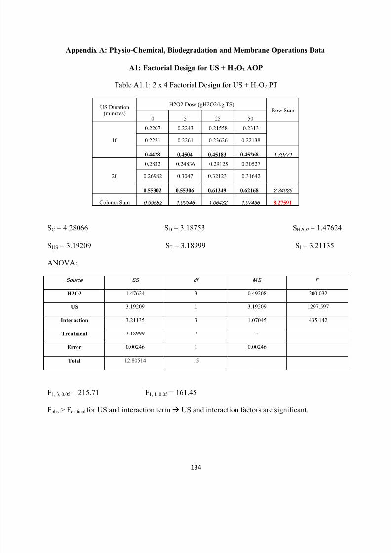
8/10/2019 Joshi Priyanka
http://slidepdf.com/reader/full/joshi-priyanka 150/166
134
Appendix A: Physio-Chemical, Biodegradation and Membrane Operations Data
A1: Factorial Design for US + H2O2 AOP
Table A1.1: 2 x 4 Factorial Design for US + H 2O2 PT
US Duration(minutes)
H2O2 Dose (gH2O2/kg TS)Row Sum
0 5 25 50
10
0.2207 0.2243 0.21558 0.2313
0.2221 0.2261 0.23626 0.22138
0.4428 0.4504 0.45183 0.45268 1.79771
20
0.2832 0.24836 0.29125 0.30527
0.26982 0.3047 0.32123 0.31642
0.55302 0.55306 0.61249 0.62168 2.34025
Column Sum 0.99582 1.00346 1.06432 1.07436 8.27591
SC = 4.28066 SD = 3.18753 SH2O2 = 1.47624
SUS = 3.19209 ST = 3.18999 SI = 3.21135
ANOVA:
Source SS df MS F
H2O2 1.47624 3 0.49208 200.032
US 3.19209 1 3.19209 1297.597
Interaction 3.21135 3 1.07045 435.142
Treatment 3.18999 7 -
Error 0.00246 1 0.00246
Total 12.80514 15
F1, 3, 0.05 = 215.71 F1, 1, 0.05 = 161.45
Fobs > Fcritical for US and interaction term US and interaction factors are significant.

8/10/2019 Joshi Priyanka
http://slidepdf.com/reader/full/joshi-priyanka 151/166
135
A2: Statistical Analysis t-tests
T-test for Thermal PT at 170ºC
X1 = 14735 mg/L X2 = 11602.5
n1 = 2 n2 = 2
v = 2, tobs = 15.533
tcritical = t0.025, 2 = 4.30
tobs > tcritical There is significant difference between the two means.
T-test for PT 8 TCOD loss
X1 = 7657.083, S1 = 1139.612 X2 = 7122.5, S2 = 595.643
n1 = 6 n2 = 6
v = 8, tobs = 1.0183
tcritical = t0.025, 8 = 2.31
tobs < tcritical There is no significant difference between the two means.
T-test for PT 10 TCOD loss
X1 = 7420 mg/L, S1 = 332.27 mg/L X2 = 7096 mg/L, S2 = 218.96 mg/L
n1 = 6 n2 = 6
v = 9, tobs = 1.99
tcritical = t0.025, 9 = 2.26
tobs <tcritical There is no significant difference between the two means.
T-test for PT 8 ffCOD increase
X1 = 42.08 mg/L, S1 = 36.2 mg/L X2 = 895.83 mg/L, S2 = 140.15 mg/L
n1 = 6 n2 = 6
v = 6, tobs = 14.45
8/10/2019 Joshi Priyanka
http://slidepdf.com/reader/full/joshi-priyanka 152/166
136
tcritical = t0.025, 6 = 2.45
tobs >tcritical There is a significant difference between the two means.
T-test for PT 10 ffCOD increase
X1 = 85 mg/L, S1 = 25.06 mg/L X2 = 1160.42 mg/L, S2 = 104.62 mg/L
n1 = 6 n2 = 6
v = 6, tobs = 24.5
tcritical = t0.025, 6 = 2.45
tobs >tcritical There is a significant difference between the two means.
T-test for PT 8 cCOD increase
X1 = 9.16 mg/L, S1 = 8.55 mg/L X2 = 1642.92 mg/L, S2 = 292.21 mg/L
n1 = 6 n2 = 6
v = 5, tobs = 13.7
tcritical = t0.025, 5 = 2.57
tobs >tcritical There is a significant difference between the two means.
T-test for PT 10 cCOD increase
X1 = 22.92 mg/L, S1 = 9.26 mg/L X2 = 1667.5 mg/L, S2 = 356.83 mg/L
n1 = 6 n2 = 6
v = 5, tobs = 11.3
tcritical = t0.025, 5 = 2.57
tobs >tcritical There is a significant difference between the two means.
T-test for PT 8 VSS decrease
X1 = 5388.33 mg/L, S1 = 93.86 mg/L X2 = 4008.33 mg/L, S2 = 133.33 mg/L
n1 = 9 n2 = 9
8/10/2019 Joshi Priyanka
http://slidepdf.com/reader/full/joshi-priyanka 153/166
137
v = 14, tobs = 25.4
tcritical = t0.025, 14 = 2.14
tobs >tcritical There is a significant difference between the two means.
T-test for PT 8 FSS decrease
X1 = 1642.78 mg/L, S1 = 83.83 mg/L X2 = 1619.44 mg/L, S2 = 246.02 mg/L
n1 = 9 n2 = 9
v = 10, tobs = 0.27
tcritical = t0.025, 10 = 2.23
tobs <tcritical
There is no significant difference between the two means.
T-test for PT 10 VSS decrease
X1 = 5258.33 mg/L, S1 = 131.23 mg/L X2 = 2733.33 mg/L, S2 = 94.29 mg/L
n1 = 9 n2 = 9
v = 14, tobs = 46.88
tcritical = t0.025, 14 = 2.14
tobs >tcritical There is a significant difference between the two means.
T-test for PT 10 FSS decrease
X1 = 1841.67 mg/L, S1 = 108.65 mg/L X2 = 1363.89 mg/L, S2 = 100.77 mg/L
n1 = 9 n2 = 9
v = 16, tobs = 9.67
tcritical = t0.025, 16 = 2.12
tobs >tcritical There is a significant difference between the two means.
8/10/2019 Joshi Priyanka
http://slidepdf.com/reader/full/joshi-priyanka 154/166
138
T-test for PT 8 VSS/TSS decrease
X1 = 77%, S1 = 0.71% X2 = 71%, S2 = 2.6%
n1 = 9 n2 = 9
v = 9, tobs = 6.68
tcritical = t0.025, 9 = 2.26
tobs >tcritical There is a significant difference between the two means.
T-test for PT 10 VSS/TSS decrease
X1 = 74%, S1 = 1.2% X2 = 67%, S2 = 2.1%
n1 = 9 n2 = 9
v = 13, tobs = 8.68
tcritical = t0.025, 13 = 2.16
tobs >tcritical There is a significant difference between the two means.
T-test for PT 8 TKN decrease
X1 = 651.98 mg/L, S1 = 51.91 mg/L X2 = 629 mg/L, S2 = 20.8 mg/L
n1 = 6 n2 = 6
v = 6, tobs = 1.00
tcritical = t0.025, 6 = 2.45
tobs <tcritical There is no significant difference between the two means.
T-test for PT 10 TKN decrease
X1 = 673.8 mg/L, S1 = 50.52 mg/L X2 = 599.71 mg/L, S2 = 42.17 mg/L
n1 = 6 n2 = 6
v = 10, tobs = 2.76
tcritical = t0.025, 10 = 2.23
8/10/2019 Joshi Priyanka
http://slidepdf.com/reader/full/joshi-priyanka 155/166
139
tobs >tcritical There is a significant difference between the two means.
T-test for PT 8 Ammonia Increase
X1 = 18.93 mg/L, S1 = 3.94 mg/L X2 = 34.82 mg/L, S2 = 1.92 mg/L
n1 = 6 n2 = 6
v = 7, tobs = 8.88
tcritical = t0.025, 7 = 2.36
tobs >tcritical There is a significant difference between the two means.
T-test for PT 10 Ammonia increase
X1 = 25.10 mg/L, S1 = 3.96 mg/L X2 = 46.74 mg/L, S2 = 5.22 mg/L
n1 = 6 n2 = 6
v = 9, tobs = 8.09
tcritical = t0.025, 9 = 2.26
tobs >tcritical There is a significant difference between the two means.
T-test for PT 8 ON decrease
X1 = 633.06 mg/L, S1 = 35.76 mg/L X2 = 594.31 mg/L, S2 = 19.72 mg/L
n1 = 6 n2 = 6
v = 7, tobs = 1.81
tcritical = t0.025, 7 = 2.36
tobs <tcritical There is no significant difference between the two means.
T-test for PT 10 ON decrease
X1 = 648.69 mg/L, S1 = 52.935 mg/L X2 = 552.96 mg/L, S2 = 34.918 mg/L
n1 = 6 n2 = 6
v = 9, tobs = 3.69
8/10/2019 Joshi Priyanka
http://slidepdf.com/reader/full/joshi-priyanka 156/166
140
tcritical = t0.025, 9 = 2.26
tobs >tcritical There is a significant difference between the two means.
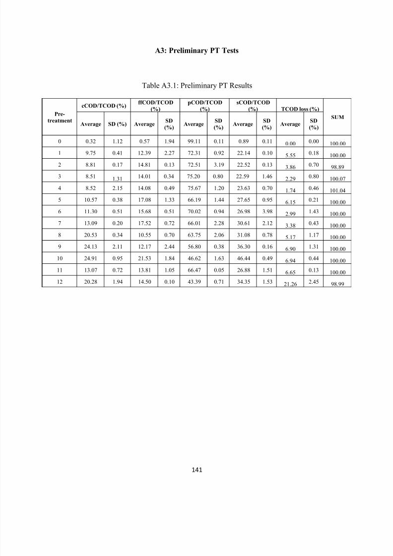
8/10/2019 Joshi Priyanka
http://slidepdf.com/reader/full/joshi-priyanka 157/166
141
A3: Preliminary PT Tests
Table A3.1: Preliminary PT Results
Pre-
treatment
cCOD/TCOD (%)ffCOD/TCOD
(%)
pCOD/TCOD
(%)
sCOD/TCOD
(%) TCOD loss (%)
SUM
Average SD (%) AverageSD
(%)Average
SD
(%)Average
SD
(%)Average
SD
(%)
0 0.32 1.12 0.57 1.94 99.11 0.11 0.89 0.11 0.00 0.00 100.00
1 9.75 0.41 12.39 2.27 72.31 0.92 22.14 0.10 5.55 0.18 100.00
2 8.81 0.17 14.81 0.13 72.51 3.19 22.52 0.13 3.86 0.70 98.89
3 8.51 1.31 14.01 0.34 75.20 0.80 22.59 1.46 2.29 0.80 100.07
4 8.52 2.15 14.08 0.49 75.67 1.20 23.63 0.70 1.74 0.46 101.04
5 10.57 0.38 17.08 1.33 66.19 1.44 27.65 0.95 6.15 0.21 100.00
6 11.30 0.51 15.68 0.51 70.02 0.94 26.98 3.98 2.99 1.43 100.00
7 13.09 0.20 17.52 0.72 66.01 2.28 30.61 2.12 3.38 0.43 100.00
8 20.53 0.34 10.55 0.70 63.75 2.06 31.08 0.78 5.17 1.17 100.00
9 24.13 2.11 12.17 2.44 56.80 0.38 36.30 0.16 6.90 1.31 100.00
10 24.91 0.95 21.53 1.84 46.62 1.63 46.44 0.49 6.94 0.44 100.00
11 13.07 0.72 13.81 1.05 66.47 0.05 26.88 1.51 6.65 0.13 100.00
12 20.28 1.94 14.50 0.10 43.39 0.71 34.35 1.53 21.26 2.45 98.99
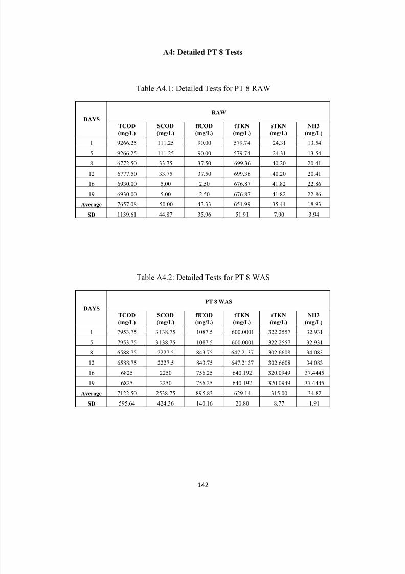
8/10/2019 Joshi Priyanka
http://slidepdf.com/reader/full/joshi-priyanka 158/166
142
A4: Detailed PT 8 Tests
Table A4.1: Detailed Tests for PT 8 RAW
DAYS
RAW
TCOD
(mg/L)
SCOD
(mg/L)
ffCOD
(mg/L)
tTKN
(mg/L)
sTKN
(mg/L)
NH3
(mg/L)
1 9266.25 111.25 90.00 579.74 24.31 13.54
5 9266.25 111.25 90.00 579.74 24.31 13.54
8 6772.50 33.75 37.50 699.36 40.20 20.41
12 6777.50 33.75 37.50 699.36 40.20 20.41
16 6930.00 5.00 2.50 676.87 41.82 22.86
19 6930.00 5.00 2.50 676.87 41.82 22.86
Average 7657.08 50.00 43.33 651.99 35.44 18.93
SD 1139.61 44.87 35.96 51.91 7.90 3.94
Table A4.2: Detailed Tests for PT 8 WAS
DAYSPT 8 WAS
TCOD
(mg/L)
SCOD
(mg/L)
ffCOD
(mg/L)
tTKN
(mg/L)
sTKN
(mg/L)
NH3
(mg/L)
1 7953.75 3138.75 1087.5 600.0001 322.2557 32.931
5 7953.75 3138.75 1087.5 600.0001 322.2557 32.931
8 6588.75 2227.5 843.75 647.2137 302.6608 34.083
12 6588.75 2227.5 843.75 647.2137 302.6608 34.083
16 6825 2250 756.25 640.192 320.0949 37.4445
19 6825 2250 756.25 640.192 320.0949 37.4445
Average 7122.50 2538.75 895.83 629.14 315.00 34.82
SD 595.64 424.36 140.16 20.80 8.77 1.91
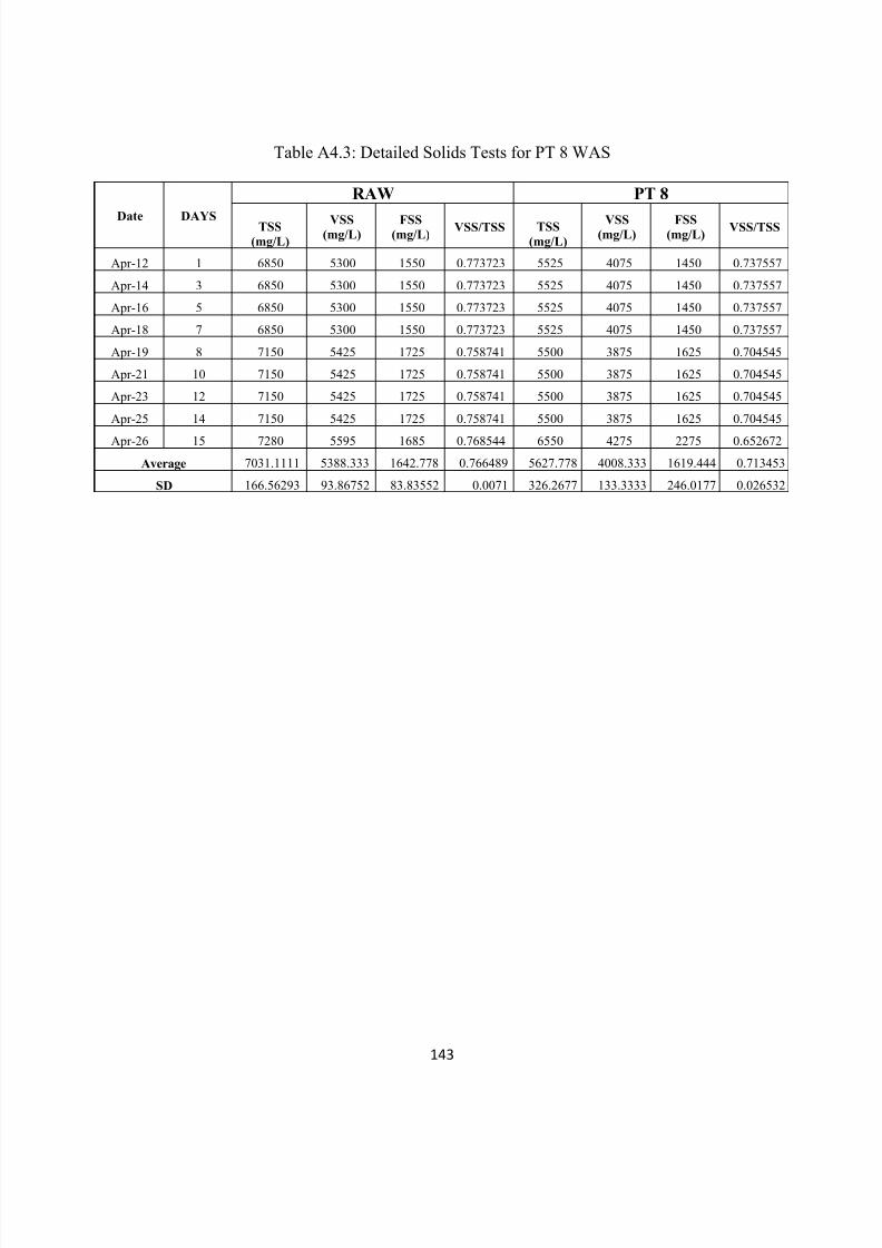
8/10/2019 Joshi Priyanka
http://slidepdf.com/reader/full/joshi-priyanka 159/166
143
Table A4.3: Detailed Solids Tests for PT 8 WAS
Date DAYS
RAW PT 8
TSS
(mg/L)
VSS(mg/L)
FSS(mg/L)
VSS/TSS TSS
(mg/L)
VSS(mg/L)
FSS(mg/L)
VSS/TSS
Apr-12 1 6850 5300 1550 0.773723 5525 4075 1450 0.737557
Apr-14 3 6850 5300 1550 0.773723 5525 4075 1450 0.737557
Apr-16 5 6850 5300 1550 0.773723 5525 4075 1450 0.737557
Apr-18 7 6850 5300 1550 0.773723 5525 4075 1450 0.737557
Apr-19 8 7150 5425 1725 0.758741 5500 3875 1625 0.704545
Apr-21 10 7150 5425 1725 0.758741 5500 3875 1625 0.704545
Apr-23 12 7150 5425 1725 0.758741 5500 3875 1625 0.704545
Apr-25 14 7150 5425 1725 0.758741 5500 3875 1625 0.704545
Apr-26 15 7280 5595 1685 0.768544 6550 4275 2275 0.652672
Average 7031.1111 5388.333 1642.778 0.766489 5627.778 4008.333 1619.444 0.713453
SD 166.56293 93.86752 83.83552 0.0071 326.2677 133.3333 246.0177 0.026532
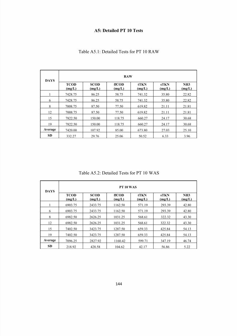
8/10/2019 Joshi Priyanka
http://slidepdf.com/reader/full/joshi-priyanka 160/166
144
A5: Detailed PT 10 Tests
Table A5.1: Detailed Tests for PT 10 RAW
DAYS
RAW
TCOD
(mg/L)
SCOD
(mg/L)
ffCOD
(mg/L)
tTKN
(mg/L)
sTKN
(mg/L)
NH3
(mg/L)
1 7428.75 86.25 58.75 741.32 35.80 22.82
6 7428.75 86.25 58.75 741.32 35.80 22.82
8 7008.75 87.50 77.50 619.82 21.11 21.81
12 7008.75 87.50 77.50 619.82 21.11 21.81
15 7822.50 150.00 118.75 660.27 24.17 30.68
19 7822.50 150.00 118.75 660.27 24.17 30.68
Average 7420.00 107.92 85.00 673.80 27.03 25.10
SD 332.27 29.76 25.06 50.52 6.33 3.96
Table A5.2: Detailed Tests for PT 10 WAS
DAYS
PT 10 WAS
TCOD
(mg/L)
SCOD
(mg/L)
ffCOD
(mg/L)
tTKN
(mg/L)
sTKN
(mg/L)
NH3
(mg/L)
1 6903.75 2433.75 1162.50 571.19 293.39 42.80
6 6903.75 2433.75 1162.50 571.19 293.39 42.80
8 6982.50 2626.25 1031.25 568.61 322.32 43.30
12 6982.50 2626.25 1031.25 568.61 322.32 43.30
15 7402.50 3423.75 1287.50 659.33 425.84 54.13
19 7402.50 3423.75 1287.50 659.33 425.84 54.13Average 7096.25 2827.92 1160.42 599.71 347.19 46.74
SD 218.92 428.58 104.62 42.17 56.86 5.22

8/10/2019 Joshi Priyanka
http://slidepdf.com/reader/full/joshi-priyanka 161/166
145
Table A5.3: Detailed Solids Tests for PT 10
Date DAYS
RAW PT 10
TSS
(mg/L)
VSS(mg/L)
FSS(mg/L)
VSS/TSS TSS
(mg/L)
VSS(mg/L)
FSS(mg/L)
VSS/TSS
Jun-07 1 7025 5100 1925 0.725979 4225 2825 1400 0.668639
Jun-09 3 7025 5100 1925 0.725979 4225 2825 1400 0.668639
Jun-12 6 7025 5100 1925 0.725979 4225 2825 1400 0.668639
Jun-13 7 7050 5300 1750 0.751773 4000 2725 1275 0.68125
Jun-14 8 7050 5300 1750 0.751773 4000 2725 1275 0.68125
Jun-16 10 7050 5300 1750 0.751773 4000 2725 1275 0.68125
Jun-18 12 7050 5300 1750 0.751773 4000 2725 1275 0.68125
Jun-19 13 7050 5300 1750 0.751773 4100 2500 1600 0.609756
Jun-21 15 7575 5525 2050 0.729373 4100 2500 1600 0.609756
Average 7100 5258.333 1841.667 0.740686 4097.222 2708.333 1388.889 0.661159
SD 168.32508 131.2335 108.6534 0.012434 98.20928 119.6058 125.339 0.028022
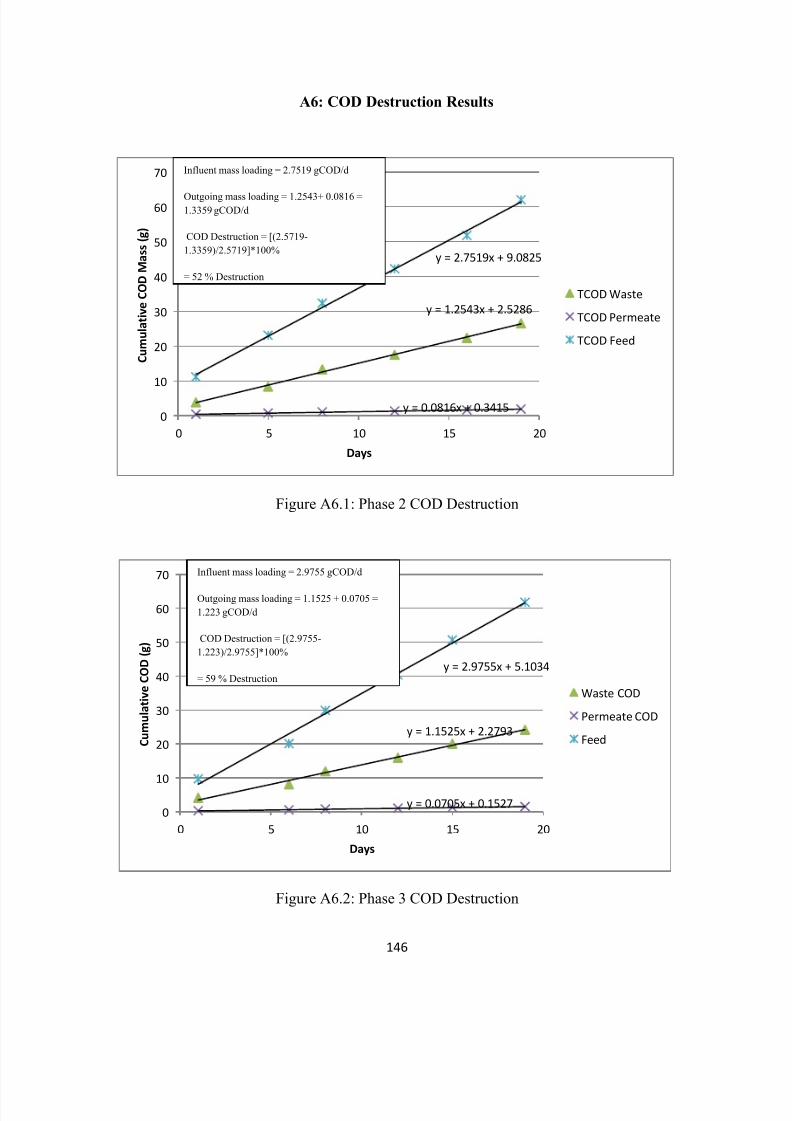
8/10/2019 Joshi Priyanka
http://slidepdf.com/reader/full/joshi-priyanka 162/166
146
A6: COD Destruction Results
Figure A6.1: Phase 2 COD Destruction
Figure A6.2: Phase 3 COD Destruction
y = 1.2543x + 2.5286
y = 0.0816x + 0.3415
y = 2.7519x + 9.0825
0
10
20
30
40
50
60
70
0 5 10 15 20
C u m u l a t i v e C O D M a s s ( g )
Days
TCOD Waste
TCOD Permeate
TCOD Feed
y = 1.1525x + 2.2793
y = 0.0705x + 0.1527
y = 2.9755x + 5.1034
0
10
20
30
40
50
60
70
0 5 10 15 20
C u m u l a t i v e C O D ( g )
Days
Waste COD
Permeate COD
Feed
Influent mass loading = 2.7519 gCOD/d
Outgoing mass loading = 1.2543+ 0.0816 =1.3359 gCOD/d
COD Destruction = [(2.5719-
1.3359)/2.5719]*100%
= 52 % Destruction
Influent mass loading = 2.9755 gCOD/d
Outgoing mass loading = 1.1525 + 0.0705 =
1.223 gCOD/d
COD Destruction = [(2.9755-
1.223)/2.9755]*100%
= 59 % Destruction
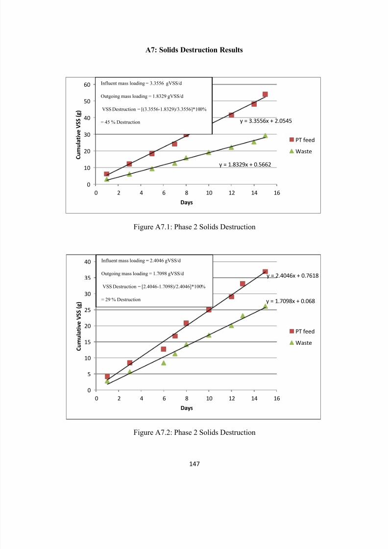
8/10/2019 Joshi Priyanka
http://slidepdf.com/reader/full/joshi-priyanka 163/166
147
A7: Solids Destruction Results
Figure A7.1: Phase 2 Solids Destruction
Figure A7.2: Phase 2 Solids Destruction
y = 3.3556x + 2.0545
y = 1.8329x + 0.5662
0
10
20
30
40
50
60
0 2 4 6 8 10 12 14 16
C u m u l a t i v e V S S ( g )
Days
PT feed
Waste
y = 2.4046x + 0.7618
y = 1.7098x + 0.068
0
5
10
15
20
25
30
35
40
0 2 4 6 8 10 12 14 16
C u m u l a t i v e V S S ( g )
Days
PT feed
Waste
Influent mass loading = 3.3556 gVSS/d
Outgoing mass loading = 1.8329 gVSS/d
VSS Destruction = [(3.3556-1.8329)/3.3556]*100%
= 45 % Destruction
Influent mass loading = 2.4046 gVSS/d
Outgoing mass loading = 1.7098 gVSS/d
VSS Destruction = [2.4046-1.7098)/2.4046]*100%
= 29 % Destruction
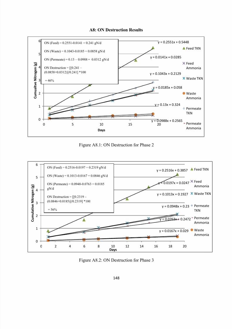
8/10/2019 Joshi Priyanka
http://slidepdf.com/reader/full/joshi-priyanka 164/166
148
A8: ON Destruction Results
Figure A8.1: ON Destruction for Phase 2
Figure A8.2: ON Destruction for Phase 3
y = 0.2551x + 0.5448
y = 0.0141x + 0.0285
y = 0.1043x + 0.2129
y = 0.0185x + 0.058
y = 0.13x + 0.324
y = 0.0988x + 0.25650
1
2
3
4
5
6
0 5 10 15 20
C u m u a l t v e N i t r o g e n ( g )
Days
Feed TKN
Feed
Ammonia
Waste TKN
Waste
Ammonia
Permeate
TKN
Permeate
Ammonia
y = 0.2516x + 0.3857
y = 0.0197x + 0.0247
y = 0.1013x + 0.1927
y = 0.0948x + 0.23
y = 0.0763x + 0.2472
y = 0.0167x + 0.029
0
1
2
3
4
5
6
0 2 4 6 8 10 12 14 16 18 20
C u m u l a t i v e N i t r o g e n ( g )
Days
Feed TKN
Feed
Ammonia
Waste TKN
Permeate
TKN
Permeate
Ammonia
WasteAmmonia
ON (Feed) = 0.2551-0.0141 = 0.241 gN/d
ON (Waste) = 0.1043-0.0185 = 0.0858 gN/d
ON (Permeate) = 0.13 – 0.0988 = 0.0312 gN/d
ON Destruction = [[0.241 –
(0.0858+0.0312)]/0.241] *100
= 46%
ON (Feed) = 0.2516-0.0197 = 0.2319 gN/d
ON (Waste) = 0.1013-0.0167 = 0.0846 gN/d
ON (Permeate) = 0.0948-0.0763 = 0.0185
gN/d
ON Destruction = [[0.2319 –
(0.0846+0.0185)]/0.2319] *100
= 56%
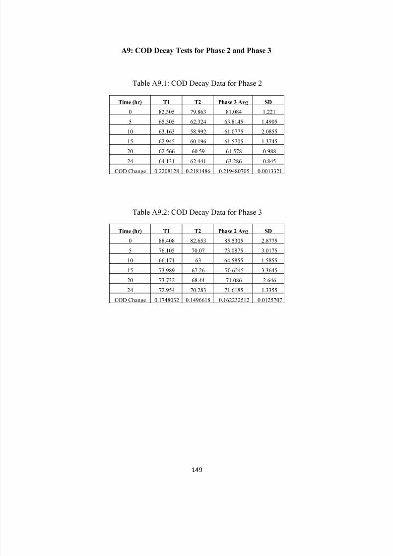
8/10/2019 Joshi Priyanka
http://slidepdf.com/reader/full/joshi-priyanka 165/166
149
A9: COD Decay Tests for Phase 2 and Phase 3
Table A9.1: COD Decay Data for Phase 2
Time (hr) T1 T2 Phase 3 Avg SD
0 82.305 79.863 81.084 1.221
5 65.305 62.324 63.8145 1.4905
10 63.163 58.992 61.0775 2.0855
15 62.945 60.196 61.5705 1.3745
20 62.566 60.59 61.578 0.988
24 64.131 62.441 63.286 0.845
COD Change 0.2208128 0.2181486 0.219480705 0.0013321
Table A9.2: COD Decay Data for Phase 3
Time (hr) T1 T2 Phase 2 Avg SD
0 88.408 82.653 85.5305 2.8775
5 76.105 70.07 73.0875 3.0175
10 66.171 63 64.5855 1.5855
15 73.989 67.26 70.6245 3.3645
20 73.732 68.44 71.086 2.646
24 72.954 70.283 71.6185 1.3355COD Change 0.1748032 0.1496618 0.162232512 0.0125707
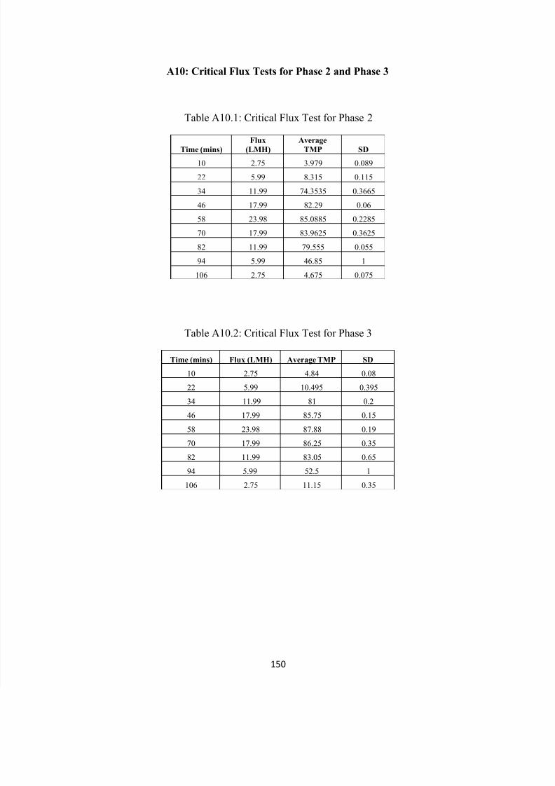
8/10/2019 Joshi Priyanka
http://slidepdf.com/reader/full/joshi-priyanka 166/166
A10: Critical Flux Tests for Phase 2 and Phase 3
Table A10.1: Critical Flux Test for Phase 2
Time (mins)Flux
(LMH)Average
TMP SD
10 2.75 3.979 0.089
22 5.99 8.315 0.115
34 11.99 74.3535 0.3665
46 17.99 82.29 0.06
58 23.98 85.0885 0.2285
70 17.99 83.9625 0.3625
82 11.99 79.555 0.055
94 5.99 46.85 1
106 2.75 4.675 0.075
Table A10.2: Critical Flux Test for Phase 3