Embed Size (px)
Citation preview

8/3/2019 Jon Paul Lundquist- Radar Sensing of Ultra-High Energy Cosmic Ray Showers
http://slidepdf.com/reader/full/jon-paul-lundquist-radar-sensing-of-ultra-high-energy-cosmic-ray-showers 1/43
RADAR SENSING OF ULTRA-HIGH ENERGY
COSMIC RAY SHOWERS
by
Jon Paul Lundquist
A Senior Honors Thesis Submitted to the Faculty of
the University of Utahin Partial Fulfillment of the Requirements for the
Honors Degree of Bachelor of Science
in
Physics
APPROVED:
John Belz David KiedaSupervisor Chair, Physics
John DeFord Martha S. BradleyDepartmental Honors Advisor Dean, Honors College
December 15, 2009

8/3/2019 Jon Paul Lundquist- Radar Sensing of Ultra-High Energy Cosmic Ray Showers
http://slidepdf.com/reader/full/jon-paul-lundquist-radar-sensing-of-ultra-high-energy-cosmic-ray-showers 2/43
ABSTRACT
The intent of this paper is to review the history and potential importance of the use
of radar techniques in detecting the ionization columns of ultra-high energy cosmic
ray showers and give a short overview of a currently planned radar experiment at
the Telescope Array. There is much activity in cosmic ray research to study the
composition and source locations of this phenomena. Radar would be an important
addition to fluorescence and scintillation detection as it theoretically could attain
greater volume coverage and nearly the accuracy of fluorescence systems with less
infrastructure and much longer running times. The currently estimated mean echo
lifetime is on the order of 50 µs for a cosmic ray of energy 1019 eV. It is shown
that a continuous wave bi-directional radar system transmitting in the low-VHF with
a large obstruction between receiver and transmitter (such as a mountain or earth
curvature), which assures direct transmission is reduced, is the nominal configuration
and the planned radar experiment at the Telescope Array satisfies these requirements.
ii

8/3/2019 Jon Paul Lundquist- Radar Sensing of Ultra-High Energy Cosmic Ray Showers
http://slidepdf.com/reader/full/jon-paul-lundquist-radar-sensing-of-ultra-high-energy-cosmic-ray-showers 3/43
TABLE OF CONTENTS
Abstract ii
1 Introduction 1
2 Characterization of Ionization Columns 3
3 Signal Duration 8
4 Signal to Noise Ratio 12
5 Radar Experiment at Telescope Array 15
6 Conclusion 25
A AREPS Instruction 30
iii

8/3/2019 Jon Paul Lundquist- Radar Sensing of Ultra-High Energy Cosmic Ray Showers
http://slidepdf.com/reader/full/jon-paul-lundquist-radar-sensing-of-ultra-high-energy-cosmic-ray-showers 4/43
Chapter 1
Introduction
Ultra-high energy cosmic rays (UHECR’s) are those particles which are just below or
exceed the theoretical GZK[1][2] cutoff limit of 5 x 10¹⁹ eV. This limit is imposed by
the cosmic background radiation interacting with the cosmic ray particle. A number
UHECR’s have been detected over a number of years. One of the highest energy
cosmic rays recorded was 3.2 x 10²⁰ eV[3].
Figure 1.1: Fly’s Eye Experiment energy spectrum showing particle of 3.2 x10 20 eV[3]
1

8/3/2019 Jon Paul Lundquist- Radar Sensing of Ultra-High Energy Cosmic Ray Showers
http://slidepdf.com/reader/full/jon-paul-lundquist-radar-sensing-of-ultra-high-energy-cosmic-ray-showers 5/43
CHAPTER 1. INTRODUCTION 2
To put this in perspective the highest proton collision energy to be achieved by
the Large Hadron Collider (LHC) is 1.4 x 10¹³ eV[4]. That is 22.9 million times less
energetic and is only for protons; cosmic ray primary particles consist of electrons,
protons, alpha particles, all the way up to iron nuclei. When these particles hit the
atmosphere they create extensive air showers (EAS) through secondary interactions
which start when they collide with an atmospheric nucleus. These showers propagate
at the nearly the speed of light and increase in size until they reach a maximum.
This creates a column of ionized air behind a relativistic disk of particle interactions
that can be detected using radar techniques that have been used to study meteors for
many years.[5][6][7]
Figure 1.2: Diagram of EAS shower and ionization column[8]
Cosmic rays of this energy are extremely rare therefore it is of great interest to
be able to collect as much data as possible on this phenomena. UHECR’s have
implications for dark matter[9], possible standard model modifications, the inter-
galactic medium, space travel, even genetic evolution[10]. It will be shown that radar
detection of UHECR’s has the capability to increase the detection volume and running
time over fluorescence detectors.
8/3/2019 Jon Paul Lundquist- Radar Sensing of Ultra-High Energy Cosmic Ray Showers
http://slidepdf.com/reader/full/jon-paul-lundquist-radar-sensing-of-ultra-high-energy-cosmic-ray-showers 6/43
Chapter 2
Characterization of Ionization
Columns
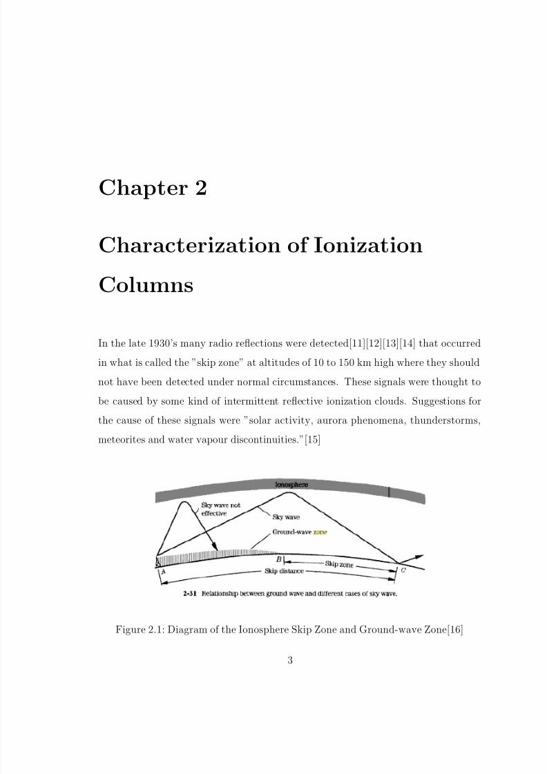
In the late 1930’s many radio reflections were detected[11][12][13][14] that occurred
in what is called the ”skip zone” at altitudes of 10 to 150 km high where they should
not have been detected under normal circumstances. These signals were thought to
be caused by some kind of intermittent reflective ionization clouds. Suggestions forthe cause of these signals were ”solar activity, aurora phenomena, thunderstorms,
meteorites and water vapour discontinuities.”[15]
Figure 2.1: Diagram of the Ionosphere Skip Zone and Ground-wave Zone[16]
3

8/3/2019 Jon Paul Lundquist- Radar Sensing of Ultra-High Energy Cosmic Ray Showers
http://slidepdf.com/reader/full/jon-paul-lundquist-radar-sensing-of-ultra-high-energy-cosmic-ray-showers 7/43
CHAPTER 2. CHARACTERIZATION OF IONIZATION COLUMNS 4
In 1940 Blackett and Lovell were the first to suggest that at least some of this
anomalous radio scattering could be explained by the ionization from extensive cosmic
ray air showers.[15] It was later shown that the signals at higher altitudes were actually
caused by meteors. This dampened interest in radar sensing of EAS for many years.[5]
This demonstrates the need to differentiate the differences between UHECR EAS
ionization columns and other types of events.
This was done in P. Gorham’s extensive treatment of radar detection of cosmic
rays[5] and what follows is a paraphrase of that paper. Radar detected meteors
generally occur at a height of 80-120 km which is also the height of lower energy
cosmic rays that are not of interest. In meteors there is an initial radius of 2-10
m and the radial ionization density is nearly uniform. The ionization column is
eventually dissipated by electron attachment and recombination. The fastest meteors
travel at approximately 100 km/s and after the meteor is depleted of material radar
echoes for frequencies from 10-100 MHz can be detectable for several seconds.[5]
Lightning ionization column charge densities are orders of magnitude higher than
either meteors or EAS and have a much smaller diameter. Therefore their radar echoes
should be longer than for EAS. They do sometimes occur in clusters transverse to the
earth at EAS maximum particle volume, X max, altitudes.[5] The X max altitude is on
average roughly 10 km for UHECR’s.[5][17]
EAS ionization columns on the other hand have a distribution that spreads out
radially as the length increases and propagates at nearly the speed of light. This
radial distribution of ionization is much more complicated than the meteor case. 90%
of the charged particles can be found within what is called the Moliere radius rm
(about 70 m at sea level) and the distribution with in this radius follows a power law.
This means that a significant amount (10%) of the ionization can be found within
less than 1% of the area of the Moliere radius or about 3.5 meters at sea level.[5] The
electron density near the core can reach above ne = 1014 m−3[6]
Blackett and Lovell[15] used a point cluster approximation where the effective

8/3/2019 Jon Paul Lundquist- Radar Sensing of Ultra-High Energy Cosmic Ray Showers
http://slidepdf.com/reader/full/jon-paul-lundquist-radar-sensing-of-ultra-high-energy-cosmic-ray-showers 8/43
CHAPTER 2. CHARACTERIZATION OF IONIZATION COLUMNS 5
number of ions is that of a column the length of the first Fresnel zone which is
dependent upon the wavelength of the incident radar. This length is[5]
L =
λR
2(2.1)
R is the distance from the shower to transmitter. They estimated that the maxi-
mum number of effective electrons per centimeter of air multiplied by L (or the total
number of effective electrons), where p is the fraction of 1 atm at the height of the
shower and E is the incident electron energy, is
N e =1
210−7 cm−1 pE
√λR (2.2)
The most important factor in characterizing the effective ionization column is the
relationship between the plasma frequency v p and the radar frequency.[5]
υ p =
nee2
4π2εome
8.98 × 10³ m3/2√ne Hz (2.3)
This is used to divide the ionization columns into two categories called overdenseand underdense ionization columns. If the electron density is high enough that v p > λ
it falls in the overdense case and the reflections will be specular or mirror-like. If
v p < λ it falls in the underdense case and the radar is able to penetrate the ionization
column. In this case the reflections are caused by coherent electron scattering and
the return power will depend quadratically on electron density. This would possibly
allow radar estimates of the energy of the primary particle by determination of the
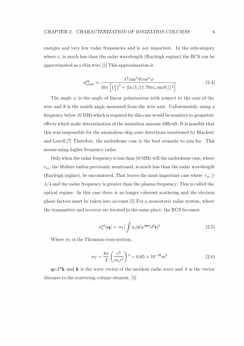
EAS electron density. [5]The effective radar cross section (RCS) for the overdense case can be approximated
as a metal cylinder with a radius rc at the point the ionization column becomes
overdense. This is where the RCS is the greatest. The case when rc is much greater
than the radar wavelength (Optical regime) is only relevant for very high shower
8/3/2019 Jon Paul Lundquist- Radar Sensing of Ultra-High Energy Cosmic Ray Showers
http://slidepdf.com/reader/full/jon-paul-lundquist-radar-sensing-of-ultra-high-energy-cosmic-ray-showers 9/43
CHAPTER 2. CHARACTERIZATION OF IONIZATION COLUMNS 6
energies and very low radar frequencies and is not important. In the subcategory
where rc is much less than the radar wavelength (Rayleigh regime) the RCS can be
approximated as a thin wire.[5] This approximation is
σodb,maz
λ2 tan2 θ cos4 φ
16π
π2
2+ (ln [λ /(1.78πrc sin θ) ]) 2
(2.4)
The angle φ is the angle of linear polarization with respect to the axis of the
wire and θ is the zenith angle measured from the wire axis. Unfortunately, using a
frequency below 10 MHz which is required for this case would be sensitive to geometric
effects which make determination of the ionization amount difficult. It is possible that
this was responsible for the anomalous skip zone detections mentioned by Blackett
and Lovell.[7] Therefore, the underdense case is the best scenario to aim for. This
means using higher frequency radar.
Only when the radar frequency is less than 10 MHz will the underdense case, where
rm, the Moliere radius previously mentioned, is much less than the radar wavelength
(Rayleigh regime), be encountered. That leaves the most important case where rm ≥λ/4 and the radar frequency is greater than the plasma frequency. This is called the
optical regime. In this case there is no longer coherent scattering and the electron
phase factors must be taken into account.[5] For a monostatic radar system, where
the transmitter and receiver are located in the same place, the RCS becomes
σudb (q) = σT |
ne(r)eiq∗rd3r|2 (2.5)
Where σT is the Thomson cross section,
σT =8π
3
e2
mec2
2 = 6.65 × 10⁻²⁹m2 (2.6)
q=2*k and k is the wave vector of the incident radio wave and r is the vector
distance to the scattering volume element. [5]

8/3/2019 Jon Paul Lundquist- Radar Sensing of Ultra-High Energy Cosmic Ray Showers
http://slidepdf.com/reader/full/jon-paul-lundquist-radar-sensing-of-ultra-high-energy-cosmic-ray-showers 10/43
CHAPTER 2. CHARACTERIZATION OF IONIZATION COLUMNS 7
The ionization density pattern can be further characterized using the NKG
approximation[18][19] to find the RCS. The conclusion is that ionization density is
highly concentrated within .5 m at 10 km for horizontal showers and for total reflection
the highest radar frequencies are 10-50MHz.[5]
The underdense optical regime, which again is the most important for the ioniza-
tion columns of UHECR EAS, can be parameterized in the case of a horizontal EAS
by [5]
σudb (10 km) = 175 f
30 MHz−1.84
E
1020
eV
1.9
R
10 kmm2 (2.7)
σudb (5 km) = 1400
f
30 MHz
−1.15
E
1020 eV
1.9R
10 km
m2 (2.8)
For normal incidence and oblique angles from 60◦ to 120◦ the radar cross section
is graphed for frequencies from 10 to 50 MHz for a UHECR of E = 1020 eV
Figure 2.2: Range of RCS at 10 km for a cosmic ray of E= 1020 eV [5]

8/3/2019 Jon Paul Lundquist- Radar Sensing of Ultra-High Energy Cosmic Ray Showers
http://slidepdf.com/reader/full/jon-paul-lundquist-radar-sensing-of-ultra-high-energy-cosmic-ray-showers 11/43
Chapter 3
Signal Duration
The exact echo signal duration for EAS ionization columns, to this date, appears to
be controversial. Ionization column duration must be long enough for a standalone
system pulsing on a set frequency, or a radar system triggered by a fluorescence or
scintillator detector, to reflect a signal off of it. If the ionization column lifetime is
too short then a pulse system will not work and a continuous wave system would have
to be considered.[5][6]
In 1940 Blackett and Lovell stated that the signal duration is the lifetime of free
electronic ions. This is dependent on the rate of molecule attachment and is ”roughly
inversely proportional to the pressure, and will have a value of 10−5 to 10−6 sec at
ground level and of the order of a second at 100 km.” Also, the amplitude times the
duration is constant, so the higher the cosmic ray the less amplitude the echo will
have.[15] The conclusion is that the signal duration would be on the order of t = .1
sec at 10 km.
In 1968 T. Matano, et al [20] stated that the collision mean time of electrons is
about 10−9 sec, the electron mean lifetime is about 10−7 sec, and the recombination
of positive and negative ions is several minutes. It was intended that to increase the
received echo power 104 radar pulses would be reflected from the EAS column in the
several minutes before recombination completes and the entire RCS dissipates.
8
8/3/2019 Jon Paul Lundquist- Radar Sensing of Ultra-High Energy Cosmic Ray Showers
http://slidepdf.com/reader/full/jon-paul-lundquist-radar-sensing-of-ultra-high-energy-cosmic-ray-showers 12/43
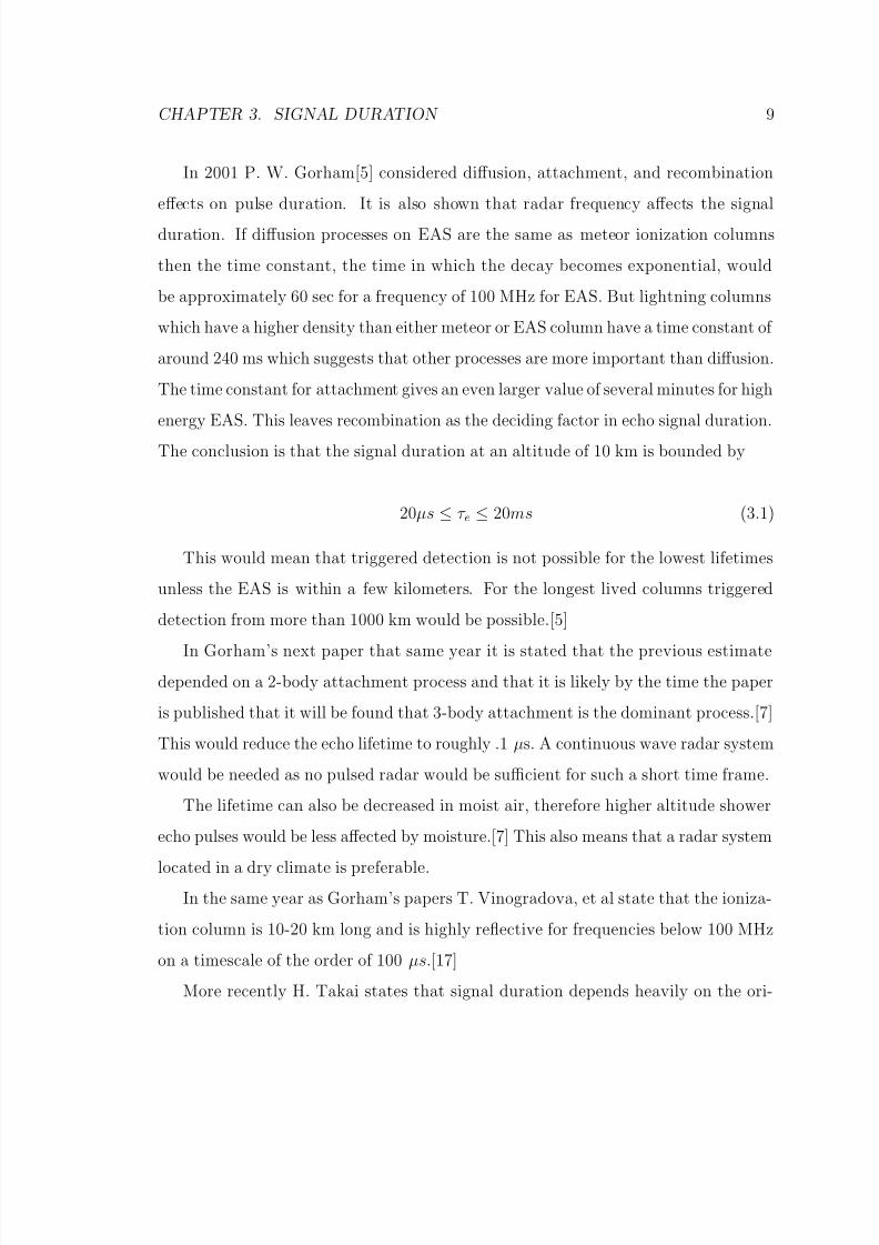
CHAPTER 3. SIGNAL DURATION 9
In 2001 P. W. Gorham[5] considered diffusion, attachment, and recombination
effects on pulse duration. It is also shown that radar frequency affects the signal
duration. If diffusion processes on EAS are the same as meteor ionization columns
then the time constant, the time in which the decay becomes exponential, would
be approximately 60 sec for a frequency of 100 MHz for EAS. But lightning columns
which have a higher density than either meteor or EAS column have a time constant of
around 240 ms which suggests that other processes are more important than diffusion.
The time constant for attachment gives an even larger value of several minutes for high
energy EAS. This leaves recombination as the deciding factor in echo signal duration.
The conclusion is that the signal duration at an altitude of 10 km is bounded by
20µs ≤ τ e ≤ 20ms (3.1)
This would mean that triggered detection is not possible for the lowest lifetimes
unless the EAS is within a few kilometers. For the longest lived columns triggered
detection from more than 1000 km would be possible.[5]
In Gorham’s next paper that same year it is stated that the previous estimatedepended on a 2-body attachment process and that it is likely by the time the paper
is published that it will be found that 3-body attachment is the dominant process.[7]
This would reduce the echo lifetime to roughly .1 µs. A continuous wave radar system
would be needed as no pulsed radar would be sufficient for such a short time frame.
The lifetime can also be decreased in moist air, therefore higher altitude shower
echo pulses would be less affected by moisture.[7] This also means that a radar system
located in a dry climate is preferable.In the same year as Gorham’s papers T. Vinogradova, et al state that the ioniza-
tion column is 10-20 km long and is highly reflective for frequencies below 100 MHz
on a timescale of the order of 100 µs.[17]
More recently H. Takai states that signal duration depends heavily on the ori-

8/3/2019 Jon Paul Lundquist- Radar Sensing of Ultra-High Energy Cosmic Ray Showers
http://slidepdf.com/reader/full/jon-paul-lundquist-radar-sensing-of-ultra-high-energy-cosmic-ray-showers 13/43
CHAPTER 3. SIGNAL DURATION 10
entation of the ionization column. Only a part of the EAS will be scattering radio
waves at any given time and the total signal time is the integration over these seg-
ments. The shortest and longest signals are those moving towards or away from the
receiver. The figure 5 shows these cases as a function of inclination angle α for the
two extreme cases of the azmithal angle β measured at the EAS tail with respect to
the transmitter. The conclusion is the signals would be between about 1 to 68 µs[6]
Figure 3.1: Range of signal durations between two extreme cases[6]
This year T. Terasawa, et al, stated that EAS echo duration should be on the order
of L/c + te. Where L is the Fresnel length and te is the lifetime of free electrons.They state that Gorham’s estimation is far too long and should likely be several µs
or shorter.[8] Their estimate is roughly 2 to 4 µs based on the te value given by R. J.
Vidmar in 1990.[21]
What can be seen from this discussion is that the important factor is the mean
electron lifetime and the length of the ionization column. Signal duration will also be
8/3/2019 Jon Paul Lundquist- Radar Sensing of Ultra-High Energy Cosmic Ray Showers
http://slidepdf.com/reader/full/jon-paul-lundquist-radar-sensing-of-ultra-high-energy-cosmic-ray-showers 14/43
CHAPTER 3. SIGNAL DURATION 11
dependent on shower direction, angle, and air moisture. It is clear that at this time a
radar experiment would need to find coincidences between echo signals and detected
events from a more proven method such as fluorescence or scintillator detectors for
a conclusive statement about signal lifetimes. Taking out the outliers and averaging
they will likely be roughly on the order of 50 µs.

8/3/2019 Jon Paul Lundquist- Radar Sensing of Ultra-High Energy Cosmic Ray Showers
http://slidepdf.com/reader/full/jon-paul-lundquist-radar-sensing-of-ultra-high-energy-cosmic-ray-showers 15/43
Chapter 4
Signal to Noise Ratio
For a monostatic system, where the antenna is at the same position as the transmitter,
P. Gorham[7] calculated the signal-to-noise ratio (SNR) to be
P rP N
= σbP tηG2λ2
(4π)3R4
1
k Tsys∆f (4.1)
The radar return power is P r, P t is the peak transmitted power, and the directivity
gain is G, σb is the effective radar backscatter cross-section given earlier, R is the
range, and lastly η is the efficiency of the transmitter-receiver system.[7] The noise
power is given by
P n = k Tsys∆f (4.2)
where k is the Boltzmann constant, ∆f is the receivers effective bandwidth, and
T sys is the system noise temperature. If echo signal durations are long enough, mul-
tiple pulses can be averaged to increase the SNR. The ratio can be multiplied by
approximately√
N which is the square root of the number of pulses used to interro-
gate the EAS.[7] The signal to noise ratio can be optimized by using the lowest radar
frequency that is possible taking into consideration background noise while also stay-
ing within the underdense regime. Just over 50 MHz is nominal in a remote area
12

8/3/2019 Jon Paul Lundquist- Radar Sensing of Ultra-High Energy Cosmic Ray Showers
http://slidepdf.com/reader/full/jon-paul-lundquist-radar-sensing-of-ultra-high-energy-cosmic-ray-showers 16/43
CHAPTER 4. SIGNAL TO NOISE RATIO 13
where the system temperature when given by
T sys = 2.9 × 10⁶
f 3MHz
−2.9
K (4.3)
is 621 K for 55.25 MHz. Parameterizing equation 4.1 gives
S
N = 3.3
σb
1m2
P t1kW
η
0.1
G
10
2λ
3m
2 R
104m
−4
T sys
103K
−1
∆t
10µs
(4.4)
where ∆t is the transmitted pulse duration.[7]According to H. Takai [6] for a bi-static radar system, where the antenna is at
the other side of the EAS from the transmitter, while taking into account that only a
part of the EAS is reflecting radio waves at a given time, and that therefore the SNR
will depend upon EAS orientation, the received power P r can be written as
dA = A0(s)κ(h)sinωt
−RR
c− φ (RT , RR) q0(s)e
−
t−
RR
c
τ (h)
H (s)ds (4.5)
for Thomson scattering at each shower segment. κ(h) is thermalization attenu-
ation, τ (h) is the free electron lifetime, h is altitude, φ(RT , RR) is the phase of the
wave at the receiving antenna and H(s) is the Heaviside function indicating that the
segment radiates only when created. A(s) is the scattering amplitude for each seg-
ment and is similar to the first half of equation 4.1 but is for the bi-static case and is
separated into components of transmitter and receiver.[6]
A(s) =
2Z in
P T GT
4πR2T
σe
4πR2R
GRλ2
4π
1/2 (4.6)
Z in is the ”electron cloud power density”[6] and σe is the single electron scattering
cross section given in equation 4.7. r2e is the classical electron radius and γ is ”the

8/3/2019 Jon Paul Lundquist- Radar Sensing of Ultra-High Energy Cosmic Ray Showers
http://slidepdf.com/reader/full/jon-paul-lundquist-radar-sensing-of-ultra-high-energy-cosmic-ray-showers 17/43
CHAPTER 4. SIGNAL TO NOISE RATIO 14
angle between the electric field of the incoming wave at the scattering center and the
vector that connects to R.”[6]
σe = 4πr2e sin2 γ (4.7)
A graph is given of the dependence on azimuthal angle for a receiver 100 km from
a 50 kW transmitter and a shower of E=1019. Four different inclinations are shown.
Both antenna have G = 10 in this case.[6]
Figure 4.1: Received power dependence on azimuthal angle of a shower of E=1019 forfour different inclinations.[6]
8/3/2019 Jon Paul Lundquist- Radar Sensing of Ultra-High Energy Cosmic Ray Showers
http://slidepdf.com/reader/full/jon-paul-lundquist-radar-sensing-of-ultra-high-energy-cosmic-ray-showers 18/43
Chapter 5
Radar Experiment at Telescope
Array
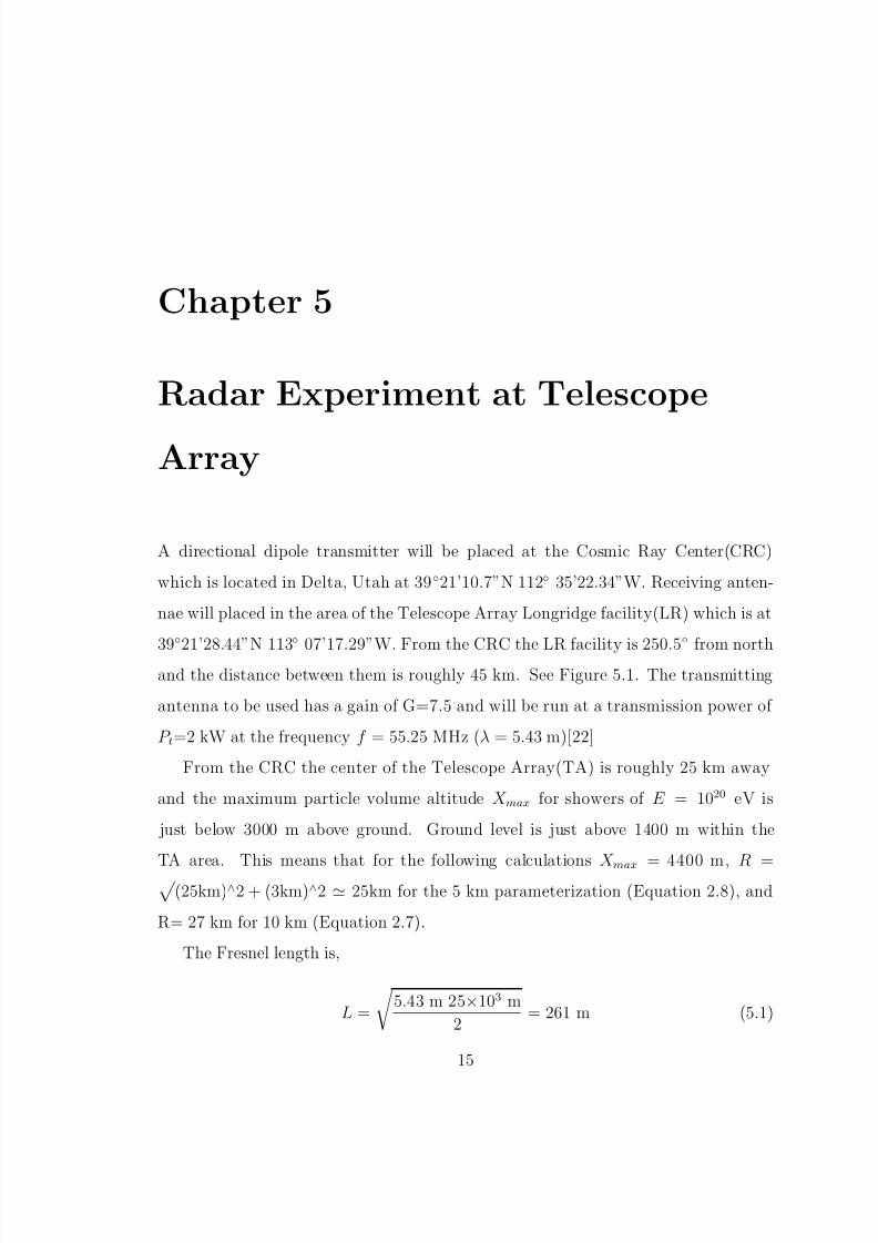
A directional dipole transmitter will be placed at the Cosmic Ray Center(CRC)
which is located in Delta, Utah at 39◦21’10.7”N 112◦ 35’22.34”W. Receiving anten-
nae will placed in the area of the Telescope Array Longridge facility(LR) which is at
39
◦
21’28.44”N 113
◦
07’17.29”W. From the CRC the LR facility is 250.5
◦
from northand the distance between them is roughly 45 km. See Figure 5.1. The transmitting
antenna to be used has a gain of G=7.5 and will be run at a transmission power of
P t=2 kW at the frequency f = 55.25 MHz (λ = 5.43 m)[22]
From the CRC the center of the Telescope Array(TA) is roughly 25 km away
and the maximum particle volume altitude X max for showers of E = 1020 eV is
just below 3000 m above ground. Ground level is just above 1400 m within the
TA area. This means that for the following calculations X max = 4400 m, R = (25km)∧2 + (3km)∧2 25km for the 5 km parameterization (Equation 2.8), and
R= 27 km for 10 km (Equation 2.7).
The Fresnel length is,
L =
5.43 m 25×103 m
2= 261 m (5.1)
15

8/3/2019 Jon Paul Lundquist- Radar Sensing of Ultra-High Energy Cosmic Ray Showers
http://slidepdf.com/reader/full/jon-paul-lundquist-radar-sensing-of-ultra-high-energy-cosmic-ray-showers 19/43
CHAPTER 5. RADAR EXPERIMENT AT TELESCOPE ARRAY 16
Figure 5.1: Diagram of angle from north of the LR facility at the CRC.
Where p=.513 at 4400 m[24] the total number of effective electrons is (Equation
2.2),
N e =1
210−7 cm−1 · .513 · 1020 · 261 m = 7 × 10¹⁶ (5.2)
The Moliere radius is[25],
rm = 74
po p
m = 144 m (5.3)
Therefore, the electron density at the radius which comprises 1% of the area of
the disc and within which 10% of the electrons are located, is,
ne =.1 · 7 × 1016
π
144 m20
2261 m
= 1.6 × 10¹³ m−3 = 1.6 × 105 cm−3 (5.4)
Then the plasma frequency v p
is (Equation 2.3),
υ p = 8.98 × 10³ m3/2√
1.6× 105 cm−3 Hz = 3.6 MHz (5.5)
This ensures that a radar of frequency of 55.25 MHz will completely penetrate a
shower of E = 1020 eV over TA. This situation is squarely in the underdense optical

8/3/2019 Jon Paul Lundquist- Radar Sensing of Ultra-High Energy Cosmic Ray Showers
http://slidepdf.com/reader/full/jon-paul-lundquist-radar-sensing-of-ultra-high-energy-cosmic-ray-showers 20/43
CHAPTER 5. RADAR EXPERIMENT AT TELESCOPE ARRAY 17
Figure 5.2: Transmitting antenna and antenna radiation pattern.[23]
case because rm ≥ λ/4 and f > υ p.
Referring to equations 2.7 and 2.8 the results for the radar cross section at altitudes
of 4.4 and 10 km are,
σudb (5 km) = 1400
55.25MHz
30 MHz
−1.15
1020 eV
1020 eV
1.925 km
10 km
m2 = 1734 m2 (5.6)
σud
b(10 km) = 17555.25MHz
30 MHz−1.841020 eV
1020 eV
1.9
27 km
10 kmm2 = 154 m2 (5.7)
For a monostatic configuration we can use equation 4.4 to find the estimated
signal to noise ratio. This can also be considered bi-static from the center of TA only
if the receiver and transmitter happen to have the same gain and system noise. The
system noise is estimated based on the noise spectrum recorded at the CRC using a

8/3/2019 Jon Paul Lundquist- Radar Sensing of Ultra-High Energy Cosmic Ray Showers
http://slidepdf.com/reader/full/jon-paul-lundquist-radar-sensing-of-ultra-high-energy-cosmic-ray-showers 21/43
CHAPTER 5. RADAR EXPERIMENT AT TELESCOPE ARRAY 18
6-element Yagi antenna.[22]
Figure 5.3: Noise spectrum recorded at the CRC using a 6-element Yagi antenna.[22]
The system temperature for f = 55.25 MHz is given by[26],
T sys = 290 ·
10log(NoiseFactor) − 1
= 290 ·
101og(30) − 1
= 8410K (5.8)
This value is greater than that estimated by equation 4.3.
For a horizontal EAS at 4400 m,
S
N = 3.3
1734m2
1m2
2 kW
1 kW
0.1
0.1
7.5
10
25.43m
3m
225km
104m
−4
8410K
103K
−1 = 64.20
(5.9)
For a horizontal EAS at 10 km,
S
N = 5.26 (5.10)
These values are far more than sufficient to see a signal from such a UHECR
EAS. For a bistatic case the gains and system temperatures will be different. Also the
system efficiency will likely be less than .1 and most EAS will not be exactly horizontal

8/3/2019 Jon Paul Lundquist- Radar Sensing of Ultra-High Energy Cosmic Ray Showers
http://slidepdf.com/reader/full/jon-paul-lundquist-radar-sensing-of-ultra-high-energy-cosmic-ray-showers 22/43
CHAPTER 5. RADAR EXPERIMENT AT TELESCOPE ARRAY 19
right in the middle of TA. Therefore these values can be considered maximums and
the real ratios will be less.
To minimize direct transmission from transmitter to receiver the receivers will be
placed behind an obstruction. A simulation was done using the Advanced Refractive
Effects Prediction System (AREPS)[27] made by the U.S. Navy which shows the
signal attenuation as it travels over the Telescope Array. AREPS uses the Advanced
Propagation Model which is a hybrid ray-optic and parabolic equation model. Figure
5.4 shows the areas that AREPS uses these different models.
Figure 5.4: Advanced Propagation Model component diagram. Bottom left is thetransmitter location and the brown area is ground.[27]
In the following figure 5.5 the transmitter attenuation is shown for the transmit-
ter at a great height using the verticle antenna pattern. No ground information is
included to demonstrate atmospheric effects.
In the next set of figures ground information is added and the transmitter is moved
closer to the ground to show ground effects.
The final diagram (Figure 5.9) is with the transmitter at the likely elevation of
50 ft above ground. In this configuration the transmitter power is relatively uniform

8/3/2019 Jon Paul Lundquist- Radar Sensing of Ultra-High Energy Cosmic Ray Showers
http://slidepdf.com/reader/full/jon-paul-lundquist-radar-sensing-of-ultra-high-energy-cosmic-ray-showers 23/43
CHAPTER 5. RADAR EXPERIMENT AT TELESCOPE ARRAY 20
Figure 5.5: Transmitter attenuation in db over TA with no ground information in-cluded. Each color change is a loss of 10db.
directly over TA at X max with a loss of 90 to 100 db from the original signal. The
received signal at Longridge on the other hand will have an estimated powerl loss of
about 155 db. This means that the EAS probing signal strength will be a factor of
106 more powerful than the direct signal received which ensures that the direct signal
should be well below the noise floor. This should be an excellent system configuration.

8/3/2019 Jon Paul Lundquist- Radar Sensing of Ultra-High Energy Cosmic Ray Showers
http://slidepdf.com/reader/full/jon-paul-lundquist-radar-sensing-of-ultra-high-energy-cosmic-ray-showers 24/43
CHAPTER 5. RADAR EXPERIMENT AT TELESCOPE ARRAY 21
Figure 5.6: Transmitter attenuation in db over TA with ground information included.Transmitter elevation of 7650 ft.

8/3/2019 Jon Paul Lundquist- Radar Sensing of Ultra-High Energy Cosmic Ray Showers
http://slidepdf.com/reader/full/jon-paul-lundquist-radar-sensing-of-ultra-high-energy-cosmic-ray-showers 25/43
CHAPTER 5. RADAR EXPERIMENT AT TELESCOPE ARRAY 22
Figure 5.7: Transmitter attenuation in db over TA with ground information included.Transmitter elevation of 5550 ft.

8/3/2019 Jon Paul Lundquist- Radar Sensing of Ultra-High Energy Cosmic Ray Showers
http://slidepdf.com/reader/full/jon-paul-lundquist-radar-sensing-of-ultra-high-energy-cosmic-ray-showers 26/43
CHAPTER 5. RADAR EXPERIMENT AT TELESCOPE ARRAY 23
Figure 5.8: Transmitter attenuation in db over TA with ground information included.Transmitter elevation of 200 ft above ground.

8/3/2019 Jon Paul Lundquist- Radar Sensing of Ultra-High Energy Cosmic Ray Showers
http://slidepdf.com/reader/full/jon-paul-lundquist-radar-sensing-of-ultra-high-energy-cosmic-ray-showers 27/43
CHAPTER 5. RADAR EXPERIMENT AT TELESCOPE ARRAY 24
Figure 5.9: Transmitter attenuation in db over TA. Transmitter elevation of 50 ftabove ground.

8/3/2019 Jon Paul Lundquist- Radar Sensing of Ultra-High Energy Cosmic Ray Showers
http://slidepdf.com/reader/full/jon-paul-lundquist-radar-sensing-of-ultra-high-energy-cosmic-ray-showers 28/43
Chapter 6
Conclusion
Because the radar echo lifetime is as yet unknown it may be too short for pulsed radar,
thus a continuous wave radar system should be run in conjunction with a fluorescence
or scintillation detection system. To maximize echo lifetimes a dry location would be
needed. A bi-directional radar system should be used for maximum detection volume
and reduction of ground wave interference. This will also allow better characterization
of energy and shower orientation. A configuration with a large obstruction between
receiver and transmitter (such as a mountain or earth curvature), which assures di-
rect transmission is reduced, is preferable. Lastly, a fairly powerful transmitter should
be run at just over 50 MHz to avoid direct reflection and difficulties with geometric
effects. This will also allow a relatively strong SNR in a remote location. Transmit-
ting radar over the Telescope Array within these parameters should present an ideal
system.
25

8/3/2019 Jon Paul Lundquist- Radar Sensing of Ultra-High Energy Cosmic Ray Showers
http://slidepdf.com/reader/full/jon-paul-lundquist-radar-sensing-of-ultra-high-energy-cosmic-ray-showers 29/43
Bibliography
[1] Greisen, K. End to the cosmic-ray spectrum? Physical Review Letters, 16(17):
748, 1966.
[2] Kuz’min, V. A., and Zatsepin, G. T. Upper limit of the spectrum of cosmic rays.
Journal of Experimental and Theoretical Physics Letters, 4:78, 1966.
[3] Bird, D.J., et al. The cosmic-ray energy spectrum observed by the Fly’s Eye.
Astrophysical Journal , 424:491, 1994.
[4] CERN Communication Group. Cern faq. http://cdsmedia.cern.ch/img/CERN-
Brochure-2008-001-Eng.pdf , January 2008, Retrieved November 16th 10:34PM.
[5] Gorham, P. W. On the possibility of radar detection of ultra-high energy cos-
mic ray- and neutrino-induced air showers. Proceedings of the Royal Society of
London. Series A. Mathematical and Physical Sciences, 15:177, 2001.
[6] Takai, H. On forward scattering extensive air shower bi-static radar. Preprint
submitted to Elsevier , 2008.
[7] Gorham, P. W. On radar detection of EeV air showers. First International work-
shop on the radio detection of high energy particles, AIP Conference proceedings ,
579:253, 2001.
26

8/3/2019 Jon Paul Lundquist- Radar Sensing of Ultra-High Energy Cosmic Ray Showers
http://slidepdf.com/reader/full/jon-paul-lundquist-radar-sensing-of-ultra-high-energy-cosmic-ray-showers 30/43
BIBLIOGRAPHY 27
[8] Terasawa, T., Nakamura, T., Sagawa, H., Miyamoto, H., Yoshida, H.,
Fukushima, M. Search for radio echoes from eas with the mu radar, shigaraki,
japan. Proceedings of the 31st ICRC, LODZ , 2009.
[9] Yoshida, S. and Sigl, G. and Lee, S. . Extremely high energy neutrinos, neutrino
hot dark matter, and the highest energy cosmic rays. Physical Review Letters,
81(25):5505, 1998.
[10] Blakely, E. A. Biological effects of cosmic radiation: Deterministic and stochastic.
Health Physics: The Radiation Safety Journal , 79:495, 2000.
[11] Colwell, R. C., and Friend, A. W. The lower ionosphere. Physical Review , 50:
632, 1936.
[12] Watson Watt, R. A., Bainbridge-Bell, L. H., Wilkins, A. F., Bowen, E. G. Return
of radio waves from the middle atmosphere. Nature, 137:866, 1936.
[13] Watson Watt, R. A., Bainbridge-Bell, L. H., Wilkins, A. F., Bowen, E. G. The
return of radio waves from the middle atmosphere. Proceedings of the Royal Society of London. Series A. Mathematical and Physical Sciences, 161:181, 1936.
[14] Appleton, E. V., and Piddington, J. H. The reflexion coefficients of ionospheric
regions. Proceedings of the Royal Society of London. Series A. Mathematical and
Physical Sciences, 164:467, 1937.
[15] Blackett, P.M.S., and Lovell, A.C.B. Radio echos and cosmic ray showers. Pro-
ceedings of the Royal Society of London. Series A. Mathematical and Physical
Sciences, 177:183, 1940.
[16] Joseph J. Carr. Practical Antenna Handbook Fourth Edition . The McGraw Hill
Companies Inc., 2001.

8/3/2019 Jon Paul Lundquist- Radar Sensing of Ultra-High Energy Cosmic Ray Showers
http://slidepdf.com/reader/full/jon-paul-lundquist-radar-sensing-of-ultra-high-energy-cosmic-ray-showers 31/43
BIBLIOGRAPHY 28
[17] Vinogradova, T., Chapin, E., Gorham, P., Saltzberg, D. Proposed experiment to
detect air showers with the jicamarca radar system. First International workshop
on the radio detection of high energy particles, AIP Conference proceedings, 579:
271, 2001.
[18] Kamata, K., and Nishimura, J. The lateral and the angular structure functions
of electron showers. Progress of Theoretical Physics Supplement , 6:93, 1958.
[19] Greisen, K. Progress in Cosmic Ray Physics, 3:Ed: Wilson, J.G. North Holland,
1965.
[20] Matano, T., Nagano, M., Suga, K., Tanahashi, G. Tokyo large air shower project.
Canadian Journal of Physics, 46:S255, 1968.
[21] Vidmar, R.J. On the use of atmospheric pressure plasmas as electromagnetic
reflectors and absorbers. IEEE Transactions on Plasma Science, 18(4):733, 1990.
[22] Belz, J.W., Takai, H., Thompson, G. Project Proposal to the NSF. 2009.
[23] KATHREIN-Werke KG. K52348. Directional Antenna 47...88 MHz.
http://www.kathrein.de//en/bca/products/download/936A753b.pdf , 2009, Re-
trieved August 26th 3:24 PM.
[24] LMNO Engineering. Static Pressure Calculation.
http://www.lmnoeng.com/Statics/pressure.htm , Last updated 2001, Retrieved
November 25th 4:41 AM.
[25] Suprun, D.A., Gorham, P.W., Rosner, J.L. Synchrotron radiation at radio fre-
quencies from cosmic ray air showers. Astroparticle Physics, 20(2):157, 2003.
[26] Satellite Signals. Noise temperature, Noise Figure and Noise Factor.
http://www.satsig.net/noise.htm , Last updated 25 March 2007, Retrieved
November 25th 4:41 AM.

8/3/2019 Jon Paul Lundquist- Radar Sensing of Ultra-High Energy Cosmic Ray Showers
http://slidepdf.com/reader/full/jon-paul-lundquist-radar-sensing-of-ultra-high-energy-cosmic-ray-showers 32/43
BIBLIOGRAPHY 29
[27] U.S. Navy Atmospheric Propagation Branch. AREPS Program. Last updated
03 September 2009, Retrieved November 25th 7:11 AM.

8/3/2019 Jon Paul Lundquist- Radar Sensing of Ultra-High Energy Cosmic Ray Showers
http://slidepdf.com/reader/full/jon-paul-lundquist-radar-sensing-of-ultra-high-energy-cosmic-ray-showers 33/43

8/3/2019 Jon Paul Lundquist- Radar Sensing of Ultra-High Energy Cosmic Ray Showers
http://slidepdf.com/reader/full/jon-paul-lundquist-radar-sensing-of-ultra-high-energy-cosmic-ray-showers 34/43
APPENDIX A. AREPS INSTRUCTION 31
Figure A.1: Starting screen
A.2 Input EM System Parameters
a) Enter the project name in the ”Project Label” area. I chose ”TA Transmit-
ter.”
Figure A.2: Project label
Next is the ”EM system parameters” section.
b) For ”Frequency (MHz)” enter the center operating frequency of the trans-
mitter. The value for our current transmitter is 55.25Mhz.
c) The ”Vertical beam width” is the vertical width of the antenna main beam.
Leave this at the default of 3 Degrees. This makes no visible difference on the
end data at the range of the Telescope Array.
d) ”Antenna elevation angle” is the direction of the maximum radiated power
and is measured from the local horizontal and increases in an upward direction.
8/3/2019 Jon Paul Lundquist- Radar Sensing of Ultra-High Energy Cosmic Ray Showers
http://slidepdf.com/reader/full/jon-paul-lundquist-radar-sensing-of-ultra-high-energy-cosmic-ray-showers 35/43
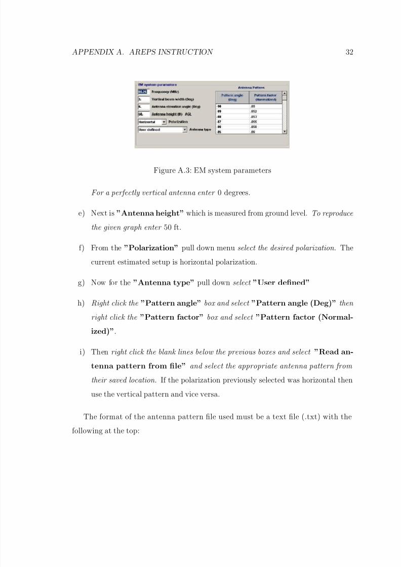
APPENDIX A. AREPS INSTRUCTION 32
Figure A.3: EM system parameters
For a perfectly vertical antenna enter 0 degrees.
e) Next is ”Antenna height” which is measured from ground level. To reproduce
the given graph enter 50 ft.
f) From the ”Polarization” pull down menu select the desired polarization. The
current estimated setup is horizontal polarization.
g) Now for the ”Antenna type” pull down select ”User defined”
h) Right click the ”Pattern angle” box and select ”Pattern angle (Deg)” then
right click the ”Pattern factor” box and select ”Pattern factor (Normal-
ized)”.
i) Then right click the blank lines below the previous boxes and select ”Read an-
tenna pattern from file” and select the appropriate antenna pattern from
their saved location. If the polarization previously selected was horizontal then
use the vertical pattern and vice versa.
The format of the antenna pattern file used must be a text file (.txt) with the
following at the top:

8/3/2019 Jon Paul Lundquist- Radar Sensing of Ultra-High Energy Cosmic Ray Showers
http://slidepdf.com/reader/full/jon-paul-lundquist-radar-sensing-of-ultra-high-energy-cosmic-ray-showers 36/43
APPENDIX A. AREPS INSTRUCTION 33
AntennaType = ”(put antenna type name here)”
AngleUnits = deg
FactorUnits = normalized
0 1.000
The first number is the angle and the second is the power factor for that angle.
The angles specified must only be from 90 to -90 degrees and can be in any order.
A.3 Selecting the APM (Advanced PropagationModel) Properties
The next section is the APM (Advanced Propagation Model) area.
a) Check the ”Include troposcatter” box and select ”Full coverage mode.”
The other modes are not appropriate for accurate calculations directly above
the Telescope Array.
Figure A.4: APM parameters
b) Below ”Full coverage mode” are two boxes to input how many data points
to calculate. The recommend input values are the maximum number of range
output points which is 1440 and the maximum number of height output points
8/3/2019 Jon Paul Lundquist- Radar Sensing of Ultra-High Energy Cosmic Ray Showers
http://slidepdf.com/reader/full/jon-paul-lundquist-radar-sensing-of-ultra-high-energy-cosmic-ray-showers 37/43
APPENDIX A. AREPS INSTRUCTION 34
which is 10000. The maximum number does not take an inordinate amount of
time on modern computers.
A.4 Selecting Environmental inputs
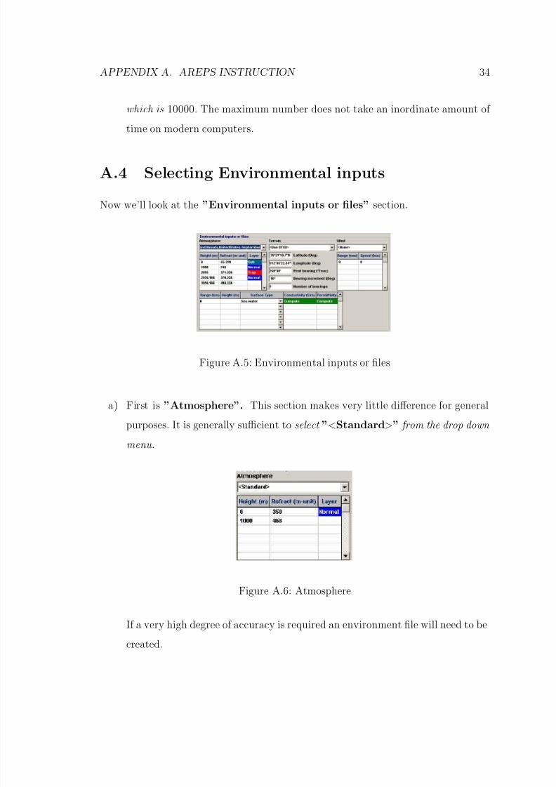
Now we’ll look at the ”Environmental inputs or files” section.
Figure A.5: Environmental inputs or files
a) First is ”Atmosphere”. This section makes very little difference for general
purposes. It is generally sufficient to select ”<Standard>” from the drop down
menu.
Figure A.6: Atmosphere
If a very high degree of accuracy is required an environment file will need to be
created.

8/3/2019 Jon Paul Lundquist- Radar Sensing of Ultra-High Energy Cosmic Ray Showers
http://slidepdf.com/reader/full/jon-paul-lundquist-radar-sensing-of-ultra-high-energy-cosmic-ray-showers 38/43
APPENDIX A. AREPS INSTRUCTION 35
b) To create an environment file click on the icon on the bar at the top.
c) In the new window that appears select ”Upper air Climatology.” ”Surface
Climatology” is only data for the first few meters above ground.
Figure A.7: Environment creator menu
d) Next select the month and ”Ely/Yelland, Nevada, United States” (which
is the closest included data to TA). Then save the environment file.
e) Now to use the environment file created select the file from the drop down menu
in the ”Environmental inputs” section in the main AREPS program window.
Next input data into the ”Terrain” subsection.
f) Select ”<Use DTED>” from the drop down menu.
g) Then input the coordinates for the transmitter position in decimal form. For a
transmitter positioned at the Cosmic Ray Center(CRC) at 39◦21’10.7”N 112◦
35’22.34”W this is 39.352972 for ”Latitude (Deg)” and -112.589538 for ”Lon-
gitude (Deg)”.
h) In the box titled ”Bearing increment (Deg)” input the number of degrees
from north that will make an intersecting line from the transmitter to the re-
ceiver. From the CRC to the Longridge site this is about 250.5 or 250◦30’.

8/3/2019 Jon Paul Lundquist- Radar Sensing of Ultra-High Energy Cosmic Ray Showers
http://slidepdf.com/reader/full/jon-paul-lundquist-radar-sensing-of-ultra-high-energy-cosmic-ray-showers 39/43
APPENDIX A. AREPS INSTRUCTION 36
Figure A.8: Terrain
i) The wind section can be ignored completely.
A.5 Input Display Options
Figure A.9: Display options
Pictured above are the nominal settings for transmitting from the CRC to Lon-
gridge. 1400 meters is the elevation at the CRC. 3500 meters is just above X max and
60 meters is just a bit farther than the distance from CRC to Longridge. To input
the values in meters (and have meters displayed in the final product):
a) Select ”Options” > ”Program Flow” from the menu bar.

8/3/2019 Jon Paul Lundquist- Radar Sensing of Ultra-High Energy Cosmic Ray Showers
http://slidepdf.com/reader/full/jon-paul-lundquist-radar-sensing-of-ultra-high-energy-cosmic-ray-showers 40/43

8/3/2019 Jon Paul Lundquist- Radar Sensing of Ultra-High Energy Cosmic Ray Showers
http://slidepdf.com/reader/full/jon-paul-lundquist-radar-sensing-of-ultra-high-energy-cosmic-ray-showers 41/43
APPENDIX A. AREPS INSTRUCTION 38
===== Files required =====
4 DTED files required for project.
W005\N28.DT1: Swap to CD: DTED144W005\N29.DT1: Swap to CD: DTED144
W006\N28.DT1: Swap to CD: DTED144
W006\N29.DT1: Swap to CD: DTED144
c) To download the indicated files go to http://edcsns17.cr.usgs.gov/EarthExplorer/
and create an account by clicking on ”Register” at the top of the page.
d) Under the ”Select your dataset(s)” section select ”Digital Elevation” and
check the box next to ”SRTM”.
Figure A.11: Dataset selection
e) In the ”Area Selected” section click the and select one corner of the area
on the Google map and then do the same for the opposite corner. Then click
”Search”.
Now that the search results are listed we’re interested in only 3-arc reso-
lution files. The ”Entity ID” corresponds to the file name. The first
example file needed W005\N28.DT1 corresponds to an ”Entity ID” of
SRTM3N28W005.

8/3/2019 Jon Paul Lundquist- Radar Sensing of Ultra-High Energy Cosmic Ray Showers
http://slidepdf.com/reader/full/jon-paul-lundquist-radar-sensing-of-ultra-high-energy-cosmic-ray-showers 42/43
APPENDIX A. AREPS INSTRUCTION 39
f) To download the example file click on ”SRTM3N28W005” then log in using
your account information .
g) Then download it into the AREPS directory ∼/AREPS30/DATA/Dted/w005.
The last subdirectory corresponds to the end of the file name.
h) When all of the required files have been saved once again click on . Then
you will see something like pictured on the following page:
Figure A.12: The Final Product − Coverage Display
i) If you would like to use the data points for other purposes right click the graph
and select ”Save all APM data in ASCII text format”.

8/3/2019 Jon Paul Lundquist- Radar Sensing of Ultra-High Energy Cosmic Ray Showers
http://slidepdf.com/reader/full/jon-paul-lundquist-radar-sensing-of-ultra-high-energy-cosmic-ray-showers 43/43
Name of Candidate: Jon Paul Lundquist
Birth Date:01 August 1980
Birth Place: Chicago, IL
Address: 180 C ST APT 9, Salt Lake City, UT