Embed Size (px)
Citation preview

Joint Return and Volatility Timing in Exchange
Traded Funds: Evidence from Tokyo Market
by
Xiaodan Gu
A research project submitted in partial fulfillment of
the requirements for the degree of Master of Finance
Saint Mary’s University
Copyright by Xiaodan Gu 2013
Written for MFIN 6692.0 under the direction of Dr. F.Boabang
Approved: Dr.F.Boabang
Faculty Advisor
Approved: Dr.F.Boabang
MFin Director
August, 2013

ii
Acknowledgements
I would like to show my appreciation to my supervisor, Dr. Francis Boabang,
who helped me to complete this report. I would like to thank all the professors
in Master of Finance Program for their contributions to my knowledge. I would
like also to thank my parents and my friends for their support and
encouragement. Lastly, I would like to express my regards to all my Master of
Finance colleagues who helped me to finish this research paper.
iii
Abstract
Joint Return and Volatility Timing in Exchange Traded Funds:
Evidence from Tokyo Market
by
Xiaodan Gu
This paper tests the existence of volatility timing skills in the Tokyo ETFs
market. The historical daily data on sixty-two ETFs are collected covering the
period July 1st, 2003 to July 16th, 2013 from Bloomberg. Two methods are
used in this paper, which are OLS- and PLS- regression methods. Regression
results are then analyzed to finger out the existence of volatility timing skills of
fund managers. The first regression results show that 90% funds confirm the
existence of volatility timing skills in the Tokyo ETFs market. The second and
third show the same results as the first one. In detail, the efficiency of volatility
timing skills on ETFs improved in the Tokyo ETFs market after t September
2008 financial crisis.
August 2013

iv
Table of Contents
Chapter 1: Introduction ............................................................................... 1
1.1 Purpose of Study ............................................................................... 1
1.2 Background: ETFs and Tokyo Market ................................................ 2
1.3 Statement of Problems ...................................................................... 3
Chapter 2: Literature Review ...................................................................... 5
2.1 Significance of ETFs .......................................................................... 5
2.2 Literatures of ETFs and Volatility Timing ............................................ 6
2.3 Recent Researches on Market Volatility Timing ................................. 9
2.4 Objectives ........................................................................................ 10
Chapter 3: Data and Methodology ............................................................. 11
3.1 Modern Portfolio Theory and Capital Asset Pricing Model ................ 11
3.2 Model ............................................................................................... 12
3.3 Data Source ..................................................................................... 14
3.4 Regression Methods ........................................................................ 14
3.5 Hypotheses of Test .......................................................................... 16
Chapter 4: Results Analysis ...................................................................... 18
4.1 Data Overview ................................................................................. 18
4.2 PLS & OLS Regression Results ...................................................... 21
4.2.1 PLS Regression...................................................................... 21
4.2.2 OLS Regression ..................................................................... 22
4.3 PLS Regression Result before and after September 2008 .............. 23
Chapter 5: Conclusion ............................................................................... 26
Reference ................................................................................................... 27
Appendix: ................................................................................................... 30
v
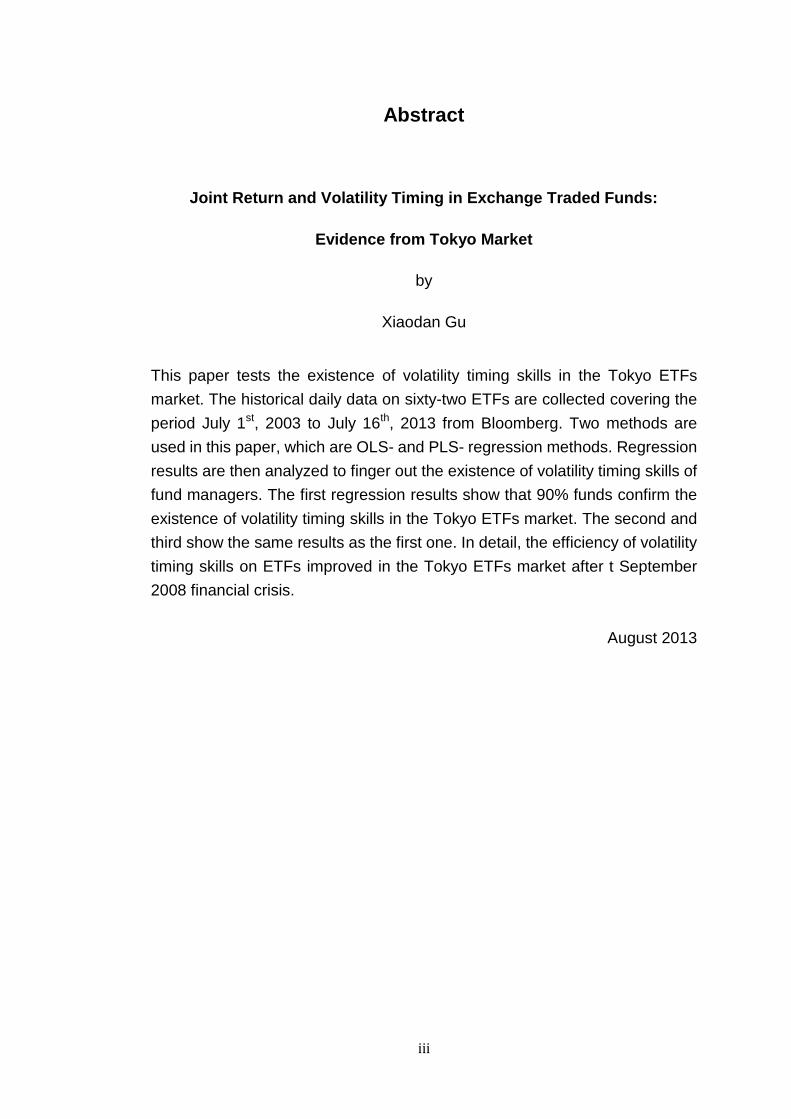
List of Table
Table 4.1: Data Summary
Table 4.2: Correlation
Table 4.3: Multi-collinearity Diagnostics
Table 4.4: PLS-Regression Results
Table 4.5: OLS-Regression Results Summery
Table 4.6: PLS-Regression Results before September 2008
Table 4.7: PLS-Regression Results after September 2008
Appendix A:
Table A.1: ETFs in Japan
Table A.2: OLS-Regression based on Volatility_10day (the whole data set)
Table A.3: OLS-Regression based on Volatility_30day (the whole data set)
Table A.4: OLS-Regression based on Volatility_60day (the whole data set)
Appendix B:
Table B.1: OLS-Regression based on Volatility_10day (data set after
September 2008)
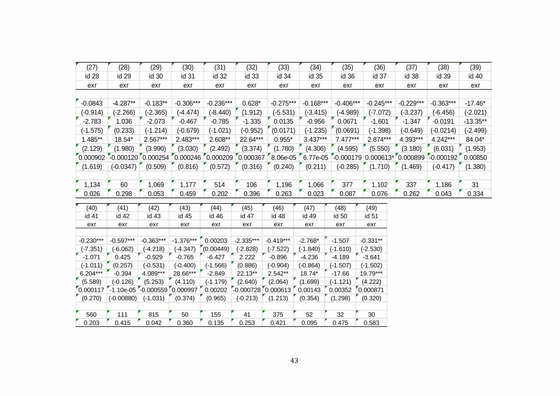
Table B.2: OLS-Regression based on Volatility_30day (data set after
September 2008)
Table B.3: OLS-Regression based on Volatility_60day (data set after
September 2008)

1
Chapter 1: Introduction
1.1 Purpose of Study
As one of the fastest growing financial products, exchange-traded fund (ETF),
has become a popular investment tool for investors all over the world’s major
securities markets over the past 15 years. ETFs are cheaper to acquire, and
provid diversification and liquidity for investors. However, the most important
factor of ETFs is that investors can get advantages of many financial products,
such as the arbitrage opportunities of index futures and commodity futures.
Therefore, ETFs could help the stock market to improve its turnover.
With the increasing numbers and styles of ETFs, investors have more options,
but have more difficulty in choosing as well. Investors would like to focus on
the performance of a fund manager, and volatility timing skill is an important
component of manager’s performance. That is, fund managers are
encouraged to appropriately forecast the overall trend of market, and
rebalance their holding portfolio to increase the return or decrease the risk.
Moreover, a lot of concerns increased after financial subprime crisis because
of the similar hedging strategy between the Collateralized Debt Obligations
(CDOs) and ETFs. Rubino (2011) summarized that financial innovations were
always faster than that of regulations. When market decides whether
derivatives should be used as the tools of risk management, though fund

2
managers’ trading skills are the factors to cause potential financial crisis, such
as ETFs, the whole chain is going to bankrupt when the primary point of
system faulting.
This report will discuss the influence of volatility timing skills on excess return
of ETFs traded in Tokyo stock markets. It will analyze the existence of timing
skills of ETFs, get a performance of the current market situation and provide
empirical suggestions to investors and financial regulators.
1.2 Background: ETFs and Tokyo Market
Since the first ETFs--SPDRs came out in the year 1993, founded by American
Stock Exchange (AMEX) and State Street, ETFs became one of the most
popular public investment tools. Until the end of July 2004, all products of
ETFs in the world were valued at $246.4 billion. Indeed, ETFs combine the
advantageous trading characteristics of closed-end fund and open-end fund,
which can both be exchanged on the secondary market, and also can be
purchased and redeemed. There are two ways to buy ETFs, by cash or using
a package of stocks. However, when it was sold or redeemed, investors
would get the basket of stocks but not cash.
Emerging from World War II in the late 60’s, Japan has held the world’s
second economic position for more than forty years, and it is the only Asian

3
country whose financial market is comparable with that in Europe and North
American. As the largest metropolitan area capital city, Tokyo is one the
biggest international financial centers and Tokyo stock market is the second
largest stock market after New York. Additionally, there are 133 ETFs traded
with a wide range of coverage in Tokyo market, which includes bond ETFs,
currency funds, dividend ETFs, inverse funds, leveraged ETFs, small-, mid-,
large-cap funds and more. According to Kennedy (n.d.), when it comes to
ETFs, Tokyo market is a very segmented and targeted market. Therefore, it is
much easier for people to investment Japanese ETFs instead of choosing a
lot of index prices and multiple broker commissions.
1.3 Statement of Problems
This report will use quantitative analysis as main method and combine
qualitative analysis, on the basis of all data and simulation constructed
selected, to prove whether volatility timing skills exists in Japanese exchange
market or not. At the same time, it is based on a wide range of relevant
literatures into describe statistical characteristics of the excess return and
volatility timing of ETFs, and verifies whether they have the same result as the
analysis from Tokyo market. Then, from the perspective of performance
attribution capacity, it measures whether volatility timing skills can bring better
results to ETFs, and whether the results are statistically significantly in
statistics test. The article will use quadratic, linear regression, correlation

4
analysis and other measurement methods, to get a relatively complete
explanation in combining excess return and volatility timing skills of ETFs
together in Tokyo market.
Chapter Two is literature review section. The details of logic inside of ETFs
will be introduced and the Modern Portfolio Theory (MPT) will be discussed;
additionally, some models in the project topic and empirical researchs of
volatility timing skills and market timing will be reviewed. Chapter Three will
introduce the methodology and the data used in this report, as well as the
underlying assumptions and suitable hypotheses. Chapter Four is outcome
analysis, Using statistic software, such as Stata and Excel, to adjust and
regress all sample data sets. From the results of the regression, it will show
the relationship of return and volatility timing in the different time periods and
forecast the optimal estimated investment. Chapter Five is conclusion of this
report.

5
Chapter 2: Literature Review
2.1 Significance of ETFs
ETFs enrich security markets greatly, because they combine advantages of
all index investments, such as lower cost, diversification, high efficiency, as
well as some other characteristics during stocks trading, such as short selling
and trading intraday. In addition, their unique system of redemption by using a
package of stocks but not cash is helpful in decreasing transaction costs and
increasing relative arbitrage activities, as well as decreasing difference of the
over- or under- price trading on the secondary market. However, the
performance in market is the most important point for an investment tool, but
not just its merits, and only the better outcome could attract more investors
and financial regulators.
Additionally, as a new investment tool in the financial market, the trading
strategies of ETFs have been used in a wide range, such as swap, leverage
and short selling. Rubino (2011) took out a question that whether ETFs will be
the new CDOs, because some fund managers use credit default swaps (CDS)
to hedge the risk of ETFs. In theory, this is an ideal trading plan to protect the
benefit of the investors and investment companies, but in the real world, it is
not “effective” enough to use. In fact, it is necessary to have a deep analysis
on ETFs, such as their operation, the performance in the market and the
demand on the financial environment.

6
2.2 Literatures of ETFs and Volatility Timing
There are some main aspects on ETFs and volatility timing skills. Firstly, the
issue of ETFs increases pricing efficiency on the stock futures indexes and
the underlying index pricing. Park and Switzer (1995) used the bank
short-term interest rate as the risk-free rate, the end of futures date as the
data date and used the daily transactions as well, they found that the pricing
mistakes of S&P 500 futures indexes decreased to a certain degree after
issuing SPDRs. Marsden and Lu (2000) used the GARCH (1,1) model to
analyze the influence of ETFs on pricing of futures indexes, and got the same
result as Switzer. Hsien and Chu (2002) considered transaction costs and the
limitations of short selling in the real investment market, to test differences of
the frequency of price deviation and arbitrage opportunities before and after
SPDRs. The results showed that futures of the S&P 500 stock index have a
close relationship with price of SPDRs. Moreover, Tian and Ackert (2001)
discussed pricing efficiency on the S&P 500 index market before and after the
exchanged of SPDRs by using put-call parity and boundary conditions theory,
the performance showed that, without conditions of limitations of short selling
and transaction costs, there was huge difference between real price and
theoretical price. Erenburg and Tse (2002), Boehmer (2003) found out that
after EFTs issued in the NYSE, transaction costs decreased and trading
efficiency increased.

7
Additionally, there are some studies on volatility timing skills. The earliest
evaluation on fund managers’ volatility timing skills was put forward by
Treynor and Mazuy (1966), which was the famous Treynor & Mazuy model
(T-M model). They concluded that expected market return was an important
factor of market timing. When expected return is high, investors should enter
the market, and choose high-risk assets; when it is low, they should leave the
market and invest in low- or no-risk assets. Meanwhile, they found out the
timing ability could follow the non-linearity regression:
( )
[( ) is used to measure market timing skills of fund managers.]
i. When is significantly positive, fund managers have good return timing
skills.
ii. When is significantly negative, fund managers have poor return timing
skills.
iii. When is equal to 0, there is no market timing activity.
After that, Henrikssin and Merton created the Henrikssin & Merton model
(H-M model) in 1984, and introduced an option-pricing theory into volatility
timing analysis at the same time. Meanwhile, they defined volatility timing
skills as fund managers’ capacity to forecast return of risk assets. The formula
is:

8
i. When is significantly positive, the market has a good
performance; when is significantly negative, the market has a
poor performance.
ii. When is significantly positive, fund managers forecast that funds have
a decreasing trend and asset allocation needs to be adjusted; when
( ) is significantly negative, fund managers have arbitrage
opportunities by short selling.
They chose 116 12-year monthly open-end funds data to do the analysis and
got an insignificant result. Therefore, they failed to prove the existence of
market timing.
Moreover, Chang and Lewellen (1984) improved the H-M model in 1984 by
using monthly data, and took out the regression model:
Where, is beta of bearish market, and is beta of bullish market.
i. When is significantly positive, fund managers have good volatility
timing skills.
ii. When is significantly negative, fund managers have poor volatility
timing skills.
They used 67 U.S monthly mutual funds data, but the outcomes still could not
prove the existence of market timing. Otherwise, the Chang & Lewellen model
(C-L model) improved studies on market timing skills. After that and for a long

9
period, all researchers could not get a significant outcome on the analysis of
market timing.
2.3 Recent Researches on Market Volatility Timing
Since the1990s, researchers began to focus on analyzing volatility timing
skills, which was another method to measure expected market return volatility
and similar to dynamics of market timing. Chou, Kroner and Bollerslev (1992)
summarized that fund managers could forecast expected market volatility
based on historical data, because they did forecast research and found out
market volatility had two characteristics, which were persistence and high
volatility. On the other hand, forecasting volatility timing is more realistic and
viable compared with market timing, because it uses more econometrical
models to forecast market return.
Ostdiek, Fleming and Korby (2000) used the short-term volatility valuation of
S&P 500 futures index to analyze the value of volatility timing on an economic
level. The report got the conclusion that the short-term volatility valuation had
a good manifestation to be used as signal of volatility timing tactics. Cao
(2011) based on CSIDM hedge fund index to test hedge funds managers’
volatility timing skills in emerging markets through the Busee model. However
his results showed that hedge funds managers were poor at using volatility
timing trading methods because of all insignificant indicators.
10
2.4 Objectives
According to previous analyses, it is obvious that market timing has a deep
relationship with volatility timing, but volatility timing skills cannot be
discussed by traditional models from the power of forecasting and the
perspective of valuation windows. Furthermore, most former research chose
hedge funds and mutual funds as the object of study, but ETFs were little
used. Meanwhile, volatility timing skills are used widely to measure a
performance of fund managers, but most data were from U.S market.
Therefore, in order to know the whole investment market well and get good
investment performance, it is necessary to have a deep analysis on volatility
timing skills for ETFs managers. At the same time, the Japanese market
holds an important financial position in the world. All in all, the main objective
of this report is to find out whether there is volatility timing in the Tokyo market
based on excess return of ETFs, especially the results in different time
periods will be showed.

11
Chapter 3: Data and Methodology
3.1 Modern Portfolio Theory and Capital Asset Pricing Model
Mitchell (2010) discussed the Modern Portfolio Theory (MPT) that was built by
Harry Markowitz in the year 1952, its core principal is that investors should
choose and rebalance the uncorrelated investments to decrease the
investment risk. There are three foundational points in this theory. The first
one is asset allocations, which choose the optimized portfolio and suitable risk
level. The second is called mean variance analysis, which developed by a
quantitative process and it helps investors to find out the most complementary
asset for a portfolio. It is more objective when analysts estimate the future
returns, standard deviations and correlations of the portfolio components,
then combining them to get an optimal return in same level of risk. The last
one is that Markowitz used the concept of optimized portfolio, which investors
should find out the best point of return and risk in a given investing
environment, financial circumstance and risk tolerance.
William Sharpe, John Lintner and Jan Mossin (1964) improved MPT into
Capital Asset Pricing Model (CAPM), whose core is to measure the
relationship between risk and expected return. CAPM is used widely even
until now, for example firms use it to estimate the cost of capital and to test the
performance of investment portfolios. The reasons are its powerfully simple
logic and intuitively predictions ability. Unfortunately, there are still limitations

12
existing because of its unrealistic hypothesis, such as all investors have the
same expected return, same correlation coefficient; there are not transaction
costs and no friction in capital market, which means all information and capital
are liquidity free and only risk-free rate could be used. Therefore, whatever
MPT or CAMP, these methods are hard to measure fund managers’ timing
skills well in real markets.
3.2 Model
Busse (1999) used the data of mutual funds’ daily return to find out the
relationship between volatility timing and excess return. The results showed
that volatility timing skills could raise the adjusted outcome ration by a certain
level of return effectively, as well as decrease exposure in the market, at the
same time, alpha and abnormal return increased significantly. However, there
are some restrictions in his model: firstly, the beta in a portfolio could be
changed when the market condition changes, but the influence time periods
are artificially adjusted. Therefore, the real result would be biased when bate
is fixed during the volatility timing tested. Secondly, it is not clarified enough in
this model for volatility timing and market timing. The last one is that uncertain
portfolio risk is existent, such as the changes in financial policy, the relevant
events, and interest risk-- even they just come from market. This report will
use the modified model built by Busse in 1999:
α β
γ
σ σ β
ε ---(1)

13
Where,
is fund daily excess return at the t time period. It is calculated by daily
return of fund subtracting the matched daily return of risk-free rate.
is fund abnormal return and it is a constant. Expected return could get by
using CAMP, but the degree of accuracy is based on the different level of
market exposure. Actually, real performance of fund always has a certain
distance with theoretical results. Fund has a negative abnormal return when
the valuation is lower than real market return, and vice versa. Hence,
could be used to measure performance of fund.
is the beta of ETFs. It describes the relationship between market and
portfolio, and shows the sensitivity degree of fund performance in market.
is daily excess return of market index at the t time period. It equals to
daily market return deducting daily risk-free rate.
is market return volatility at the t time period. It uses market return
standard deviation of pervious workday. This report will use three groups of
short-term valuation time periods: Volatility_10day, Volatility_30day and
Volatility_60day.
is average volatility of market return. It is used as the benchmark market
return and explains the level of average market return volatility in short-term
valuation time period that same as using. In addition, when is less
than , market is in a low volatility period, a good fund manager should
invest higher volatility market and short sell low volatility market.
14
is volatility timing factor. It is the most important indicator to measure
whether volatility timing exists in market. Statistic testes of the characters of
can be used to explain the existence of volatility timing skills. When it is
significantly negative, fund managers have volatility timing skills, and large
absolute value of means stronger ability.
is market timing factor. It also can measure fund managers’ volatility
timing skills, but it is different with . When is significantly positive,
fund managers have high capacity.
is the error term.
3.3 Data Source
Some ETFs in Japanese market are shown on table A.1. This report will use
10-year (from 2003-7-1 to 2013-7-16) daily returns, and 62 of 133 ETFs in the
Tokyo market are chosen, because other ETFs were issued less than 4 years.
All data is from Bloomberg. In addition, Nikkei-225 is the benchmark index
and its average 10-year daily return is used as market return (Rm). Nikkei-225
is widely used in Japan market, which is made up by the price-weighted
average of 225 tops rated companies in Japan, which listed in the Tokyo stock
market.
3.4 Regression Methods
This report will use two methods to do the regression, Ordinary Least Square

15
(OLS) and Partial Least Square (PLS), and they have own advantages and
shortcomings.
OLS is one of the most widely used method in multivariate analysis, the
reason is that OLS recognized that there could be error terms between
explanatory variables and dependent variables. OLS method is always
chosen when the relevance between explanatory variables and dependent
variables needs to be tested and parameters are unknown. The
multi-collinearity problem should be concerned, because the regression of
OLS is linear, at the same time, if the underlying model is not correct, OLS
could not provide true estimates.
On the other hand, PLS is a recent put forward regression method, which
combines and generalizes multiple regression and the characteristics of
component analysis. Its core is to analyze and forecast a set of dependent
variables from a set of predictors or independent variables (Abdi). Indeed, this
forecasting is reached through latent that is the predictors a set of orthogonal
items, which have the most powerful predictive ability. When researchers
want to forecast a set of dependent variables from a huge set of independent
variables, PLS regression method is extremely useful with a high degree of
accuracy. It is true that, combining PLS and OLS regression method is a good
way to do regression analysis in this report.
16
3.5 Hypotheses of Test
The whole data will be used to do regression at the first step, and find out
whether there is existence volatility marking skills in the Tokyo ETFs market.
After that, all data would be separated into two parts, which is based on the
data—September 2008, and two testes will be regressed, which regressed
the same way as the first step. Besides, the reason why September 2008 is
used to be the boundary of two tests is that, a world widely financial crisis
reached a critical step during the first week in September 2008. This subprime
mortgage crisis had a deep influence in the global credit market, such as
investment bank and Stock Exchanges. As one of the biggest international
financial centers, the Tokyo market could not exit from this financial disaster
successfully. Therefore, September 2008 is the separate time period since its
huge impact.
In details, the P-value of all regressions is an important factor to show the
quality of volatility timing skills. The whole historical data of ETFs would be
used in the first testing:
H0: Volatility timing skills exist in the Tokyo ETFs market.
H1: Volatility timing skills do not exist in the Tokyo ETFs market.
After the first regression, all data are separated into two parts: data before
September 2008, and data after September 2008. Another two regressions

17
will be showed, by using the same methods as the first regression.
H0’: Volatility timing skills exist in the Tokyo ETFs market before September
2008
H1’: Volatility timing skills do not exist in the Tokyo ETFs market before
September 2008.
H0’ ’: Volatility timing skills exist in the Tokyo ETFs market after September
2008.
H1’ ’: Volatility timing skills do not exist in the Tokyo ETFs market after
September 2008.

18
Chapter 4: Results Analysis
4.1 Data Overview
All original data are from Bloomberg as tables in Excel. The fixed data come
out by using different formulas, such as excess return (exr) and R square (r2).
After that, all original and fixed data are posted in Stata, which would be used
to do OLS- and PLS- regression and get tested results. Most useful tables are
shown following:
Table 4.1: Data Summary
According to table 4.1, data summary, there are almost 73 thousand data
points in the whole data set. It shows that both funds and market had good
performance with positive mean of ETFs’ return and market return during the
collected time period, 0.3038% and 0.3231% respectively. Funds’ excess
return is negative that means its performance is worse than market’s,
meanwhile its standard deviation is a little bit less than market’s, it describes
ETFs have a lower volatility level compared with benchmark. To the contrary,
k60d 52914 6.53e-06 .0013775 -.0355017 .0289912 k30d 54643 3.08e-06 .0020277 -.0760101 .075818 k10d 58192 -2.61e-06 .0026207 -.0797953 .0792242 r2 73200 .0002919 .0008684 0 .0143082 rm 73200 .0003431 .0170818 -.104651 .119617 exr 71881 -.0000393 .0169571 -.266306 .282174 id 73211 23.09172 15.55196 2 62 date 73211 40137.75 968.6143 37628 41474 Variable Obs Mean Std. Dev. Min Max

19
the Min and Max (-26.6306% & 28.2174% and -10.4651% & 11.9617%
separately) indicates that there might be volatility timing skills existing in ETFs
in the Tokyo market. In following regression, the analysis will be based on the
result of γ
that is the coefficient of σ σ . fund managers have
volatility timing skills when it is significantly negative, and larger absolute
value of means stronger ability. At the same time, three valuation
windows should be used to calculate market volatility timing, which named
k_10d, k_30d and k_60d.
Table 4.2: Correlation
Table 4.2 shows correlations of all variables from the whole data set, and
most explanatory variables have low correlations, except of k_10d, k_30d and
k_60d these three explanatory variables have a higher correlations, that
because of their similar data characters. The largest correlation with excess
return is K-10day 0.3210. Whatever which regression method is chosen,
excess return of ETFs are always the dependent variable, and the other 3
k60d 0.0041 0.0071 0.1092 0.2374 -0.0495 0.5761 0.8500 1.0000 k30d 0.0040 0.0048 0.2020 0.0792 -0.0298 0.7614 1.0000 k10d 0.0022 0.0038 0.3210 -0.1109 0.0002 1.0000 r2 -0.0001 0.0228 0.0202 -0.1170 1.0000 rm 0.0159 -0.0010 -0.2775 1.0000 exr -0.0083 -0.0030 1.0000 id 0.3835 1.0000 date 1.0000 date id exr rm r2 k10d k30d k60d

20
explanatory variables are independent variables to explain it. When all
explanatory variables have high absolute correlation with each other, the
multi-collinearity issue would happen. The regression result might look good,
but it dose make no sense in the real world when the correlations are closed
to 1 or -1. However, when it happens, OLS regression method should be
chosen, because it can make the error terms lower. Otherwise, it cannot
explain excess return of ETFs well, and that is why this report will combine
two methods together. Meanwhile, based on this table, 0.3210 is not big
enough to cause multi-collinearity problem.
Additionally, respectively using the volatility factors, Volatility_10day,
Volatility_30day and Volatility_60day to get the regression functions,
therefore, there are four functions and Variance Inflation Factor (VIF). VIF
function:
VIF= 1 / (1 – R2)
VIF is always used to measure Multi-collinearity problems in a regression
function. When it is higher than 10, it means nearly perfect Multi-collinearity;
when it is lower than 5, then data can be regard as low collinearity relationship,
which would not have serious influence on the result of regression. According
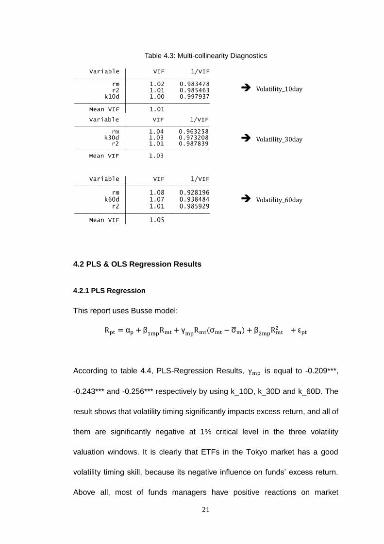
to table 4.3, the three VIFs are 1.01, 1.03, 1.05, which are all lower than 1.5,
therefore, Multi-collinearity is not a problem on all regressions.
21
Table 4.3: Multi-collinearity Diagnostics
4.2 PLS & OLS Regression Results
4.2.1 PLS Regression
This report uses Busse model:
α β
γ
σ σ β
ε
According to table 4.4, PLS-Regression Results, is equal to -0.209***,
-0.243*** and -0.256*** respectively by using k_10D, k_30D and k_60D. The
result shows that volatility timing significantly impacts excess return, and all of
them are significantly negative at 1% critical level in the three volatility
valuation windows. It is clearly that ETFs in the Tokyo market has a good
volatility timing skill, because its negative influence on funds’ excess return.
Above all, most of funds managers have positive reactions on market
Mean VIF 1.01 k10d 1.00 0.997937 r2 1.01 0.985463 rm 1.02 0.983478 Variable VIF 1/VIF
Mean VIF 1.03 r2 1.01 0.987839 k30d 1.03 0.973208 rm 1.04 0.963258 Variable VIF 1/VIF
Mean VIF 1.05 r2 1.01 0.985929 k60d 1.07 0.938484 rm 1.08 0.928196 Variable VIF 1/VIF
Volatility_10day
Volatility_30day
Volatility_60day

22
changing. When market volatility increases, they should sell high-risk asset to
decrease the risk of whole portfolio, and vice versa. Therefore, the PLS
method regression test accept hypotheses H0 that volatility timing skills do
exist in the Tokyo ETFs market.
Table 4.4: PLS-Regression Results
4.2.2 OLS Regression
Every fund would be regressed one by one by using OLS method, compared
with the former PLS method that regards all historical data as a whole data
set, OLS could show the relationship between volatility timing and ETFs’
performance individually. All regression results are showed on table A.2 to
(1) (2) (3)
r1 r2 r3
VARIABLES exr exr exr
rm -0.209*** -0.243*** -0.256***
(-34.11) (-40.23) (-43.28)
r2 0.0238 -0.0920 -0.146
(0.138) (-0.458) (-0.705)
k10d 1.413***
(19.96)
k30d 1.365***
(13.19)
k60d 1.641***
(16.79)
Constant -2.29e-05 1.07e-05 4.03e-05
(-0.374) (0.164) (0.622)
Observations 57,498 53,978 52,061
R-squared 0.145 0.112 0.108
Robust t-statistics in parentheses
*** p<0.01, ** p<0.05, * p<0.1

23
table A.4, which are on Appendix pages: they are the regression results under
volatility 10-day, volatility 30-day, and volatility 60-day data set respectively.
Table 4.5: OLS-Regression Results Summery
***1%
-
**5%
-
*10%
- Insignificantly - Insignificantly + Cumulative
Positive
γ
Volatility-
10d 46 3 2 5 3 59 3
Volatility-
30d 45 3 2 4 1 55 1
Volatility-
60d 39 4 3 2 2 50 3
Table 4.5, OLS-Regression Results Summery, is summarized according to
table A.2 to table A.4. This table shows that 79.3% (130 to 164 in total)
individual the coefficient of ETF, is significantly negative at 1% critical
level, 89.6% is significantly negative at less or equal 10% critical level, just 10%
special funds are not performance significant or have positive . In details,
most fund managers have volatility timing skills and take positive actions
when investment market changes. Obviously, the results from OLS method
have same conclusions as they from PLS method, which evident to accept
hypotheses H0 that volatility timing skills do exist in the Tokyo ETFs market.
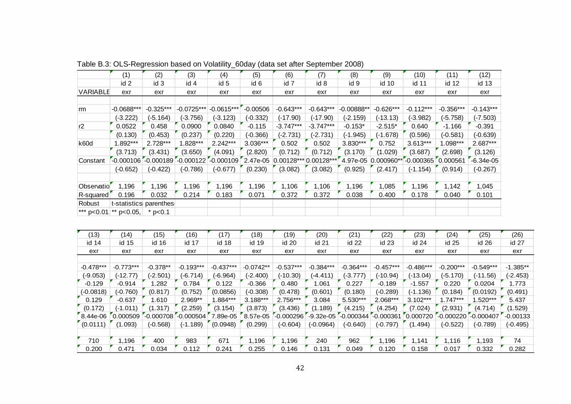
4.3 PLS Regression Result before and after September 2008
As the report talked before, all data sets are separated into two parts: before
and after the global subprime crisis in September 2008. Using PLS regression
method to regress the data before and after the date September 2008, two
results are showing on table 4.6 and table 4.7.

24
Table 4.6: PLS-Regression Results before September 2008
Table 4.7: PLS-Regression Results after September 2008
(1) (2) (3)
r1 r2 r3
VARIABLES exr exr exr
rm -0.966*** -1.183*** -1.145***
(-9.301) (-11.66) (-10.22)
r2 1.714*** 1.885*** 1.973***
(22.87) (24.83) (20.79)
key10m -2.581***
(-6.268)
key30m -2.590***
(-5.339)
key60m -4.174***
(-4.678)
Constant -0.000505*** -0.000486*** -0.000419***
(-6.597) (-6.224) (-5.543)
Observations 41,736 39,025 37,707
R-squared 0.014 0.016 0.012
t-statistics in parentheses
*** p<0.01, ** p<0.05, * p<0.1

25
According to the two tables, all s are significantly negative at 1% critical
level in the three volatility valuation windows in the two groups. All outcomes
show that the Hypotheses H0’ and H0’ ’ is accepted, which means volatility
timing skills do exist in the Tokyo ETFs market before and after September
2008. On the other hand, the absolutely value of after September 2008
is larger than it is before September 2008, it speaks volume that volatility
timing skills of fund managers improved after the separated date--
September 2008, because larger absolutely value of stands for
powerful influence on excess return.

26
Chapter 5: Conclusion
As a new investment tool recent years, ETFs play an increasingly important
role in financial market. Due to the occurrence of financial subprime crisis and
the similarity between ETFs and CDOs in hedging strategy, this paper
focuses on volatility timing skills of fund managers.
This report separates the whole data set into two parts to study the volatility
timing before and after September 2008 in ETFs. In addition, three different
valuation windows are employed into regression models, which are
Volatility_10day, Volatility_30day and Volatility_60day. The regression results
show that 90% funds in all data sets have a statistically significant coefficient
to prove the existence of volatility timing skills. When regressions are
undertaken in two separated data sets, the some results come out. Volatility
timing skill is a good factor to measure quality of funds, and numerous
methods and factors could make further studies on ETFs.
All in all, from all regression results, this report shows that volatility timing
skills do exist in the Tokyo ETFs market based on the chosen data sets. At the
same time, fund managers’ skills improved after the separated date--
September 2008

27
Reference
Amihud, Y. and R. Goyenko. (2011), Mutual fund R2 as a predictor of
performance, working paper, New York University. Retrieved from
http://www.cirano.qc.ca/realisations/grandes_conferences/prmia/2011-12-07/
R2-paper-December-2011-PRMIA.pdf
Ackert, L. F., & Tian, Y. S. (2001). Efficiency in index options markets and
trading in stock baskets. Journal of Banking & Finance, 25(9), 1607-1634.
Boehmer.B, & Boehmer, K. (2003). Trading your neighbor's ETFs:
Competition or fragmentation? Journal of Banking and Finance, forthcoming.
Bollerslev, T., R.Y. Chou, & K.F. Kroner. (1992), ARCH Modeling in Finance:
A Review of the Theory and Empirical Evidence. Journal of Econometrics,
Busse Jeffrey A. (1999). Volatility Timing in Mutual Funds: Evidence from
Daily Returns. Review of Financial Studies, 1999, (12): 1009-1041
Cao, B. (2011). Volatility Timing in the Emerging Market Hedge Funds Indices.
Retrieved from http://papers.ssrn.com/sol3/papers.cfm?abstract_id=1859683
Chang, E. C., & Lewellen, W. G. (1984). Market timing and mutual fund
investment performance. The Journal of Business (Pre-1986), 57(1), 57.
Retrieved from
http://search.proquest.com/docview/222575397?accountid=13908

28
Chu, Q.C., Wen-liang, G., & Tse, Y. (1999). Price discovery on the S&P 500
index markets: An analysis of spot index, index futures, and SPDRs.
International Review of Financial Analysis, 8(1), 21-34.
Fama, E.F (1972). Components of Investment Performance. The Journal of
Finance, 1972(3): 551-567
Henriksson, R. D. (1984). Market timing and mutual fund performance: An
empirical investigation. The Journal of Business (Pre-1986), 57(1), 73.
Retrieved from
http://search.proquest.com/docview/222600289?accountid=13908
John Rubino. (2011). Emerging Threat Funds? CFA Magazine 29
September/October 2011(22): 4-5.
Kennedy, M. (n.d.) Invest in Japan with Japanese ETFs. Exchange Traded
Funds. Retrieved from
http://etf.about.com/od/foreignetfs/a/Invest-In-Japan-With-Japanese-Etfs.htm
Lu, L. & Marsden. (2000). NZSE-10 Index Fund Units and the Market
Efficiency of the Index Futures: Evidence from the New Zealand Market.
Presented for the 7th Annual Conference of APFA, Shanghai.
Mazuy, K. & Trenynor. J. (1966). Can Mutual Funds Outguess the Market?
Harvard Buness Review, 1966, (44): 131-136

29
Mitchell, D. (2010, 08). The big bang. Financial Planning, 40, 41-n/a.
Retrieved from
http://search.proquest.com/docview/734640287?accountid=13908
N.D. (n.d.). Japan: A Spirit to Excel. Thomas white international. Retrieved
from http://www.thomaswhite.com/world-markets/japan-a-spirit-to-excel/
Park, T. H., & Switzer, L. N. (1995). Index participation units and the
performance of index futures markets: evidence from the toronto 35 index
participation units market. The Journal of Futures Markets (1986-1998), 15(2),
187.
Tse, Y., & Erenburg, G. (2003). Competition for order flow, market quality,
and price discovery in the NASDAQ 100 index tracking stock. The Journal of
Financial Research, 26(3), 301-318.
Vol.52, p.5-59.

30
Appendix A:
Table A.1: ETFs in Japan
Symbol Name Country Type Industry/Objective
1624:JP Nomura Next Funds Topix-17
Machinery Etf
Japan ETF Sector Fund-Undefined
Equity
1648:JP Daiwa Etf Topix-17 Banks Japan ETF Sector Fund-Financial
Service
9D312135:JP Simplex Nikkei225 Bear -1X Etf Japan ETF Contrarian
1613:JP Nomura Topix Electric
Appliances Exchange Traded
Fund
Japan ETF Sector Fund-Undefined
Equity
1554:JP Nikko Listed Index Fund World
Equity Msci Acwi Ex Japan
Japan ETF International Equity
1636:JP Daiwa Etf Topix-17 Construction
& Materials
Japan ETF Sector Fund-Utility
1320:JP Daiwa Etf - Nikkei 225 Japan ETF Growth-Large Cap
1649:JP Daiwa Etf Topix-17 Financials Japan ETF Sector Fund-Financial
Service
1555:JP Nikko Listed Index Fund
Australian Reit S&P/Asx200
A-Reit
Japan ETF Country Fund-Australia
1638:JP Daiwa Etf Topix-17
Pharmaceutical
Japan ETF Sector Fund-Health &
Biotech
1317:JP Nikko Listed Index Fund Topix
Mid400 Japan Mid Cap Equity
Japan ETF Growth-Mid Cap
9D31111C:JP Simplex Nikkei 225 Covered Call
Etf
Japan ETF Country Fund-Japan
1626:JP Nomura Next Funds Topix-17 It
& Services Others Etf
Japan ETF Sector Fund-Internet &
Telecom
1551:JP Simplex Jasdaq Top 20
Exchange Traded Fund
Japan ETF Country Fund-Japan
1610:JP Daiwa Etf - Topix Electric
Appliances
Japan ETF Sector Fund-Undefined
Equity
1623:JP Nomura Next Funds Topix-17
Steel & Nonferrous Etf
Japan ETF Sector Fund-Undefined
Equity
1635:JP Daiwa Etf Topix-17 Energy
Sources
Japan ETF Sector Fund-Energy
Data Source:
http://www.bloomberg.com/markets/symbolsearch?query=Japan+ETF

31
Table A.2: OLS-Regression based on Volatility_10day (the whole data set)
(1) (2) (3) (4) (5) (6) (7) (8) (9) (10) (11) (12)
id 2 id 3 id 4 id 5 id 6 id 7 id 8 id 9 id 10 id 11 id 12 id 13
VARIABLES exr exr exr exr exr exr exr exr exr exr exr exr
rm -0.0632*** -0.230*** -0.0666*** -0.0581*** -0.0134 -0.458*** -0.458*** -0.00542** -0.568*** -0.123*** -0.282*** -0.0892***
(-6.026) (-8.794) (-7.033) (-6.134) (-1.490) (-8.401) (-8.401) (-1.964) (-10.58) (-6.147) (-4.436) (-2.591)
r2 -0.0331 0.176 -0.0833 -0.153 -0.222 -1.981* -1.981* -0.0621 -1.580 0.541 0.308 0.656
(-0.0734) (0.236) (-0.177) (-0.300) (-0.641) (-1.837) (-1.837) (-0.867) (-1.221) (0.504) (0.199) (0.899)
k10d 1.168*** 2.457*** 1.229*** 1.443*** 1.742*** 1.207*** 1.207*** 2.348*** 0.749* 1.702*** 1.142** 2.280***
(4.871) (10.31) (4.513) (5.182) (4.650) (3.358) (3.358) (7.857) (1.858) (4.336) (2.558) (3.954)
Constant -1.50e-05 -6.31e-05 -1.69e-05 1.47e-05 5.72e-05 0.000940**0.000940** 2.22e-05 0.000830** -0.000129 -0.000409 -0.000385
(-0.125) (-0.215) (-0.137) (0.111) (0.650) (2.081) (2.081) (0.578) (2.059) (-0.472) (-0.643) (-1.397)
Observations 2,587 2,587 2,587 2,587 2,587 1,176 1,176 2,587 1,158 2,262 1,212 1,107
R-squared 0.187 0.090 0.200 0.193 0.123 0.304 0.304 0.088 0.384 0.165 0.078 0.190
Robust t-statistics in parentheses
*** p<0.01, ** p<0.05, * p<0.1
(13) (14) (15) (16) (17) (18) (19) (20) (21) (22) (23) (24) (25) (26)
id 14 id 15 id 16 id 17 id 18 id 19 id 20 id 21 id 22 id 23 id 24 id 25 id 26 id 27
exr exr exr exr exr exr exr exr exr exr exr exr exr exr
-0.327*** -0.711*** -0.327*** -0.134*** -0.333*** -0.0991*** -0.329*** -0.305*** -0.165*** -0.293*** -0.315*** -0.263*** -0.509*** -0.542***
(-11.10) (-15.85) (-7.185) (-5.422) (-5.505) (-5.020) (-7.190) (-4.191) (-6.538) (-9.305) (-7.301) (-3.670) (-9.158) (-6.582)
0.286 -0.987 1.491 0.591 0.300 -0.739 0.212 0.967 0.403 -0.279 0.0761 -0.487 -0.0457 1.413
(0.299) (-0.919) (1.519) (0.775) (0.222) (-0.616) (0.188) (0.590) (0.514) (-0.425) (0.0681) (-0.323) (-0.0396) (0.476)
1.005*** 0.200 2.393*** 1.613*** 1.121*** 1.644*** 1.196*** 2.244*** 1.996*** 1.634*** 2.073*** 2.169*** 0.767*** 1.536*
(3.716) (0.907) (8.325) (4.677) (4.687) (3.568) (3.451) (3.917) (8.189) (6.372) (9.304) (5.400) (3.464) (1.688)
-4.54e-05 0.000646 -0.000400 -0.000216 0.000222 0.000213 -0.000324 -0.000533 -9.26e-05 -0.000701 0.000127 -0.000101 -0.000267 -0.000661
(-0.133) (1.546) (-0.746) (-0.802) (0.326) (0.749) (-0.616) (-0.772) (-0.312) (-1.513) (0.251) (-0.204) (-0.512) (-0.449)
2,083 1,448 1,372 1,848 870 1,989 1,285 608 2,135 1,399 1,211 1,168 1,249 233
0.183 0.474 0.113 0.136 0.245 0.244 0.139 0.247 0.083 0.129 0.189 0.103 0.330 0.166

32
(27) (28) (29) (30) (31) (32) (33) (34) (35) (36) (37) (38) (39) (40) (41)
id 28 id 29 id 30 id 31 id 32 id 33 id 34 id 35 id 36 id 37 id 38 id 39 id 40 id 41 id 42
exr exr exr exr exr exr exr exr exr exr exr exr exr exr exr
-0.142* -0.445*** -0.0838 -0.448*** -0.259*** -0.327*** -0.229*** -0.0550 -0.148*** -0.203*** -0.265*** -0.151*** -0.769*** -0.178*** -0.483***
(-1.934) (-3.357) (-1.563) (-7.466) (-7.506) (-5.027) (-6.055) (-1.517) (-3.651) (-4.936) (-4.737) (-3.610) (-4.218) (-5.186) (-6.369)
-0.798 1.320 1.945* -0.719 -1.777*** -2.242 -0.102 -0.652 2.284** 0.971 0.662 -0.414 -5.204** 0.572 0.608
(-0.519) (0.407) (1.941) (-0.757) (-3.223) (-1.302) (-0.125) (-0.648) (2.115) (0.849) (0.517) (-0.377) (-2.361) (1.005) (0.351)
1.373*** 1.501 1.898*** 0.129 0.572* 2.636*** 0.997*** 1.279*** 2.009*** 1.668*** 1.250** 1.298*** 3.747*** 0.963*** 0.904
(3.678) (1.256) (5.654) (0.376) (1.858) (3.423) (4.004) (3.038) (4.198) (5.732) (2.433) (4.075) (3.266) (4.848) (1.440)
0.000512 0.000454 -0.000542 0.000321 0.000306 0.000906 2.33e-05 6.07e-05 -0.000184 -7.50e-05 0.000395 -6.33e-05 0.00287 -0.000102 -0.000223
(0.882) (0.231) (-1.124) (0.928) (0.864) (1.434) (0.0695) (0.160) (-0.379) (-0.183) (0.888) (-0.131) (1.115) (-0.281) (-0.424)
1,184 146 1,059 1,220 550 308 1,399 1,033 657 1,136 591 1,280 113 763 361
0.035 0.089 0.128 0.431 0.301 0.384 0.254 0.058 0.126 0.122 0.323 0.048 0.143 0.277 0.430
(42) (43) (44) (45) (46) (47) (48) (49) (50) (51) (52) (53) (54) (55) (56) (57) (58) (59)
id 43 id 44 id 45 id 46 id 47 id 48 id 49 id 50 id 51 id 52 id 53 id 56 id 57 id 58 id 59 id 60 id 61 id 62
exr exr exr exr exr exr exr exr exr exr exr exr exr exr exr exr exr exr
-0.236*** -0.394*** -0.241*** -0.706*** -0.303*** -0.410*** -0.345** -0.339** -0.293*** -0.429*** 0.545 -1.514*** 0.0563 0.0563 -0.231 -0.603*** -0.164 -1.274*
(-3.927) (-5.963) (-3.098) (-7.307) (-3.825) (-5.946) (-2.207) (-2.580) (-3.713) (-5.288) (0.483) (-3.374) (0.293) (0.293) (-1.539) (-2.830) (-0.451) (-2.710)
1.052 -1.569 -0.126 -4.732 3.369*** -1.308 -1.796 2.972 -3.923 -2.764 -27.95 -6.876*** 3.973 3.973 6.379 0.639 18.14 13.96
(1.158) (-0.892) (-0.109) (-1.377) (2.956) (-0.716) (-0.463) (1.573) (-1.004) (-1.453) (-0.797) (-3.051) (1.307) (1.307) (1.558) (0.0685) (1.587) (0.542)
2.729*** 3.481*** 4.311*** 1.783** 1.639** 1.211** 0.900* 0.918 1.987** 1.882*** 8.247 6.718** -3.042 -3.042 0.0279 2.223** -3.362 -4.612
(7.693) (5.336) (5.006) (2.393) (2.386) (2.377) (1.694) (0.790) (2.208) (3.240) (1.226) (2.356) (-0.794) (-0.794) (0.0199) (2.655) (-1.364) (-1.828)
-0.000571 -0.000111 8.38e-05 0.000528 -0.00398** 0.000550 0.00197 -0.00395** 0.000557 -0.000384 0.00148 0.00835* -0.00400 -0.00400 -0.00260 0.00334 -0.00434 -0.0181
(-1.195) (-0.140) (0.0586) (0.402) (-2.240) (1.206) (0.834) (-2.276) (0.397) (-0.224) (0.379) (1.692) (-1.572) (-1.572) (-0.776) (1.406) (-0.746) (-0.971)
879 306 115 345 150 620 108 126 125 151 8 44 45 45 56 28 29 7
0.130 0.163 0.294 0.104 0.169 0.440 0.054 0.199 0.226 0.169 0.600 0.377 0.118 0.118 0.090 0.443 0.374 0.656

33
Table A.3: OLS-Regression based on Volatility_30day (the whole data set)
(1) (2) (3) (4) (5) (6) (7) (8) (9) (10) (11) (12) (13)
id 2 id 3 id 4 id 5 id 6 id 7 id 8 id 9 id 10 id 11 id 12 id 13 id 14
VARIABLES exr exr exr exr exr exr exr exr exr exr exr exr exr
rm -0.0656*** -0.284*** -0.0694*** -0.0625*** -0.0140 -0.567*** -0.567*** -0.0105*** -0.583*** -0.141*** -0.309*** -0.117*** -0.358***
(-6.090) (-8.215) (-7.296) (-6.281) (-1.489) (-11.32) (-11.32) (-3.602) (-12.43) (-6.918) (-5.239) (-3.922) (-12.08)
r2 0.0266 0.883 0.0317 0.00621 -0.147 -1.126 -1.126 -0.115 -1.956 0.428 1.637 0.433 0.158
(0.0696) (1.018) (0.0838) (0.0158) (-0.467) (-0.605) (-0.605) (-1.565) (-1.596) (0.426) (1.152) (0.462) (0.156)
k30d 1.545*** 2.495*** 1.563*** 1.858*** 2.203*** 1.269* 1.269* 3.259*** 1.105* 1.906*** 0.910*** 3.131*** 1.404***
(4.913) (6.775) (4.898) (5.494) (3.986) (1.891) (1.891) (5.804) (1.910) (3.548) (2.788) (3.359) (2.859)
Constant -3.17e-05 -0.000139 -3.67e-05 -2.41e-05 3.44e-05 0.000805 0.000805 4.20e-05 0.000896** -0.000192 -0.000626 -0.000241 -1.49e-05
(-0.290) (-0.455) (-0.336) (-0.214) (0.420) (1.540) (1.540) (1.072) (2.291) (-0.741) (-0.988) (-0.814) (-0.0415)
Observations 2,587 2,587 2,587 2,587 2,587 1,158 1,158 2,587 1,140 2,176 1,194 1,082 1,963
R-squared 0.168 0.046 0.179 0.163 0.075 0.326 0.326 0.045 0.366 0.134 0.043 0.143 0.167
Robust t-statistics in parentheses
*** p<0.01, ** p<0.05, * p<0.1
(14) (15) (16) (17) (18) (19) (20) (21) (22) (23) (24) (25) (26) (27) (28)
id 15 id 16 id 17 id 18 id 19 id 20 id 21 id 22 id 23 id 24 id 25 id 26 id 27 id 28 id 29
exr exr exr exr exr exr exr exr exr exr exr exr exr exr exr
-0.785*** -0.402*** -0.173*** -0.384*** -0.118*** -0.429*** -0.381*** -0.213*** -0.388*** -0.421*** -0.259*** -0.518*** -0.586*** -0.240** -0.746***
(-17.05) (-6.525) (-7.934) (-6.153) (-5.213) (-9.000) (-4.992) (-4.668) (-10.72) (-11.54) (-6.720) (-9.660) (-4.845) (-2.234) (-2.978)
-0.960 1.415 0.610 0.0800 -0.362 0.301 -0.242 0.107 -0.337 -0.524 -0.321 -0.0746 0.389 -0.695 -0.0536
(-0.840) (1.062) (0.745) (0.0578) (-0.331) (0.300) (-0.105) (0.0939) (-0.524) (-0.547) (-0.195) (-0.0642) (0.111) (-0.461) (-0.0107)
-0.330 2.208*** 2.313*** 1.300*** 1.854*** 1.278*** 2.454** 2.685*** 1.635*** 2.675*** 1.349** 1.050*** 1.859 1.883*** 2.697*
(-1.013) (4.630) (3.674) (3.514) (3.036) (2.914) (2.176) (5.099) (5.221) (7.373) (2.185) (3.853) (1.507) (2.974) (1.875)
0.000606 -0.000160 -0.000317 0.000115 0.000136 -0.000487 0.000167 -4.95e-05 -0.000565 0.000271 -0.000190 -0.000168 -0.000302 0.000483 -0.000978
(1.380) (-0.250) (-1.098) (0.152) (0.531) (-0.988) (0.207) (-0.136) (-1.214) (0.550) (-0.371) (-0.320) (-0.139) (0.852) (-0.312)
1,430 1,112 1,687 747 1,932 1,267 404 2,012 1,381 1,193 1,154 1,220 143 1,168 95
0.475 0.048 0.118 0.212 0.224 0.134 0.150 0.045 0.103 0.171 0.041 0.325 0.136 0.021 0.136

34
(29) (30) (31) (32) (33) (34) (35) (36) (37) (38) (39) (40) (41) (42)
id 30 id 31 id 32 id 33 id 34 id 35 id 36 id 37 id 38 id 39 id 40 id 41 id 42 id 43
exr exr exr exr exr exr exr exr exr exr exr exr exr exr
-0.260** -0.462*** -0.239*** -0.379*** -0.256*** -0.0791** -0.162*** -0.234*** -0.241*** -0.267*** -0.593* -0.209*** -0.486*** -0.326***
(-2.210) (-7.007) (-8.191) (-5.096) (-6.607) (-2.542) (-3.146) (-5.813) (-4.143) (-6.015) (-1.735) (-4.617) (-5.908) (-4.849)
-2.157 -0.664 -0.292 -0.757 -0.0575 -1.700** 0.864 0.316 -1.044 -0.00894 -5.932** 0.745 -0.0905 0.0731
(-0.965) (-0.688) (-0.467) (-0.453) (-0.0700) (-2.438) (0.736) (0.262) (-0.599) (-0.00991) (-2.058) (0.819) (-0.0496) (0.0545)
2.610*** -0.0139 1.599** 1.267 0.899*** 1.780*** 3.049*** 1.460*** 3.536*** 2.636*** 2.023 1.237*** 2.056* 3.718***
(3.680) (-0.0272) (2.441) (1.348) (2.695) (3.609) (4.668) (2.785) (4.055) (5.136) (0.936) (2.820) (1.749) (6.384)
0.000101 0.000273 8.10e-05 0.00104 4.41e-05 0.000262 -0.000521 1.72e-05 0.000702 -0.000101 0.00246 -0.000401 -0.000334 -0.000615
(0.157) (0.793) (0.234) (1.383) (0.130) (0.784) (-0.948) (0.0412) (1.410) (-0.220) (0.669) (-0.878) (-0.435) (-1.145)
1,039 1,196 511 199 1,381 1,029 468 1,146 435 1,270 75 580 206 833
0.059 0.434 0.226 0.354 0.229 0.030 0.088 0.060 0.307 0.042 0.058 0.234 0.388 0.063
(43) (44) (45) (46) (47) (48) (49) (50) (51) (52) (53) (54) (55)
id 44 id 45 id 46 id 47 id 48 id 49 id 50 id 51 id 52 id 57 id 58 id 59 id 60
exr exr exr exr exr exr exr exr exr exr exr exr exr
-0.595*** -0.509*** -1.023*** -0.601* -0.320*** -0.981*** -0.536*** -0.320*** -0.991*** -1.918 -1.918 -0.274 103.7
(-4.191) (-3.676) (-6.250) (-1.818) (-4.228) (-4.006) (-3.167) (-4.054) (-3.666) (-1.503) (-1.503) (-1.217)
-2.560 2.112* -3.530 2.649 -2.429 -3.747 -1.471 -6.324 -9.219** -9.112 -9.112 -0.208 670.8
(-0.679) (1.735) (-1.235) (0.926) (-1.642) (-0.817) (-0.759) (-1.438) (-2.361) (-0.640) (-0.640) (-0.0385)
9.024** 7.936*** 3.408*** 5.118 3.107*** 5.619*** -1.034 2.854 8.232* 28.35 28.35 -3.062 -1,188
(2.494) (3.558) (3.164) (1.307) (3.197) (3.243) (-0.574) (1.520) (1.930) (1.729) (1.729) (-1.248)
0.000188 0.000645 -0.000475 -0.00524* 0.00120** 0.00310 -0.000369 0.00152 0.00173 0.000747 0.000747 0.000253 0.00348
(0.175) (0.367) (-0.285) (-1.735) (2.492) (1.055) (-0.159) (1.012) (0.428) (0.0577) (0.0577) (0.0599)
139 89 214 44 479 82 53 65 30 11 11 51 4
0.117 0.212 0.107 0.135 0.441 0.094 0.358 0.241 0.393 0.200 0.200 0.168 1.000

35
Table A.4: OLS-Regression based on Volatility_60day (the whole data set)
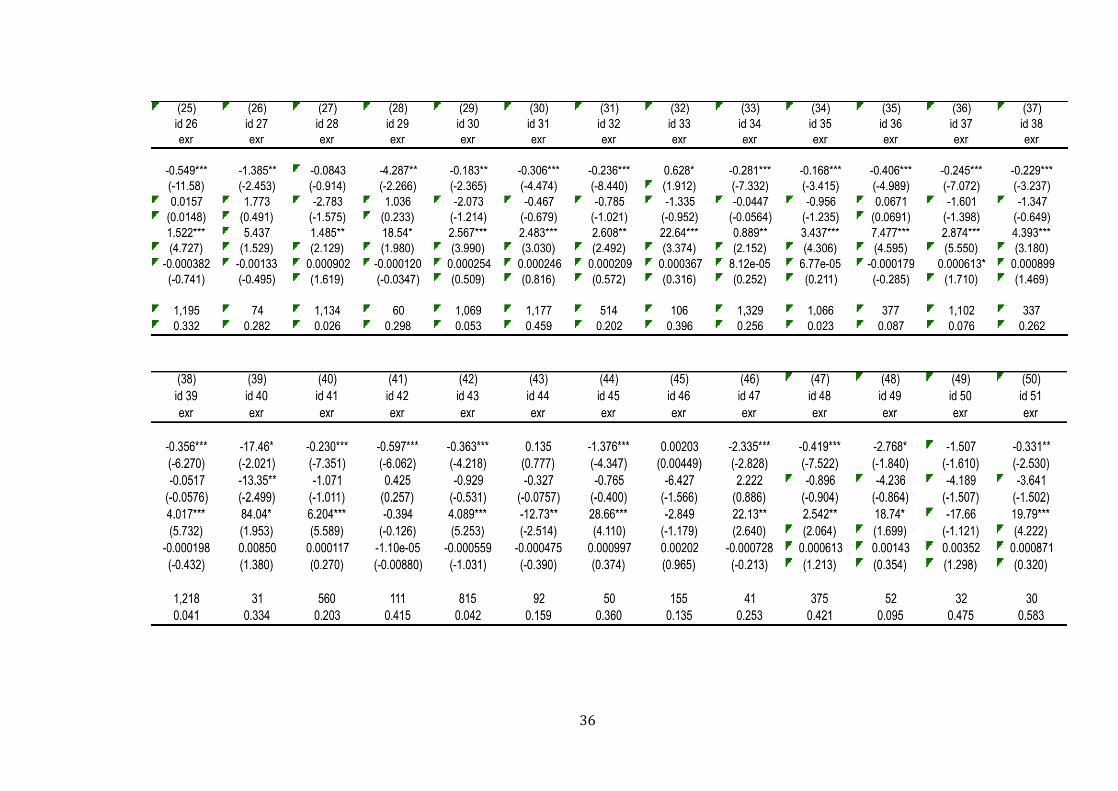
36

37
Appendix B:
Table B.1: OLS-Regression based on Volatility_10day (data set after September 2008)
(1) (2) (3) (4) (5) (6) (7) (8) (9) (10) (11) (12)id 2 id 3 id 4 id 5 id 6 id 7 id 8 id 9 id 10 id 11 id 12 id 13
VARIABLES exr exr exr exr exr exr exr exr exr exr exr exr
rm -0.0707*** -0.225*** -0.0697*** -0.0553*** -0.00589 -0.458*** -0.458*** -0.00346 -0.570*** -0.0907*** -0.275*** -0.0892***(-3.982) (-6.679) (-4.451) (-3.574) (-0.427) (-8.401) (-8.401) (-0.968) (-10.63) (-3.214) (-4.318) (-2.591)
r2 -0.00529 0.0733 -0.0237 -0.104 -0.196 -1.981* -1.981* -0.0668 -1.606 0.781 0.275 0.656(-0.0113) (0.0872) (-0.0498) (-0.204) (-0.568) (-1.837) (-1.837) (-0.909) (-1.244) (0.677) (0.177) (0.899)
k10d 0.965*** 2.170*** 1.039*** 1.245*** 1.506*** 1.207*** 1.207*** 1.946*** 0.732* 1.762*** 1.149** 2.280***(3.748) (7.269) (3.659) (4.289) (3.836) (3.358) (3.358) (5.146) (1.819) (3.776) (2.564) (3.954)
Constant -7.71e-05 -0.000175 -9.72e-05 -5.93e-05 6.45e-05 0.000940** 0.000940** 4.00e-05 0.000872** -0.000386 -0.000317 -0.000385(-0.443) (-0.408) (-0.566) (-0.322) (0.557) (2.081) (2.081) (0.770) (2.177) (-1.155) (-0.500) (-1.397)
Observations 1,196 1,196 1,196 1,196 1,196 1,176 1,176 1,196 1,155 1,196 1,196 1,107R-squared 0.220 0.103 0.244 0.224 0.138 0.304 0.304 0.101 0.388 0.229 0.080 0.190Robust t-statistics in parentheses*** p<0.01, ** p<0.05, * p<0.1
(13) (14) (15) (16) (17) (18) (19) (20) (21) (22) (23) (24) (25) (26) (27)id 14 id 15 id 16 id 17 id 18 id 19 id 20 id 21 id 22 id 23 id 24 id 25 id 26 id 27 id 28exr exr exr exr exr exr exr exr exr exr exr exr exr exr exr
-0.373*** -0.674*** -0.328*** -0.130*** -0.332*** -0.0472** -0.323*** -0.308*** -0.142*** -0.291*** -0.310*** -0.264*** -0.505*** -0.543*** -0.151**(-7.862) (-12.76) (-5.728) (-3.723) (-5.090) (-2.013) (-6.796) (-4.111) (-3.987) (-8.708) (-7.180) (-3.684) (-8.863) (-6.312) (-2.043)0.456 -0.922 1.639 0.765 0.302 -0.845 0.259 1.005 0.456 -0.157 0.0783 -0.499 -0.00617 1.416 -0.748
(0.424) (-0.815) (1.524) (0.922) (0.221) (-0.653) (0.231) (0.611) (0.540) (-0.240) (0.0704) (-0.331) (-0.00536) (0.475) (-0.484)0.718** 0.240 2.202*** 1.461*** 1.102*** 1.929*** 1.197*** 2.240*** 1.864*** 1.537*** 2.082*** 2.199*** 0.775*** 1.535* 1.478***(2.267) (1.022) (6.621) (3.794) (4.536) (3.893) (3.166) (3.884) (7.103) (5.151) (9.351) (5.410) (3.472) (1.664) (3.938)
-0.000112 0.000494 -0.000621 -0.000430 0.000429 0.000228 -0.000229 -0.000639 -0.000194 -0.000435 0.000158 -7.81e-05 -0.000371 -0.000421 0.000513(-0.165) (1.116) (-0.785) (-1.123) (0.577) (0.694) (-0.437) (-0.903) (-0.423) (-0.970) (0.309) (-0.158) (-0.697) (-0.279) (0.882)
774 1,196 645 971 759 1,196 1,196 582 979 1,196 1,195 1,162 1,192 225 1,1780.218 0.472 0.157 0.155 0.248 0.366 0.152 0.250 0.101 0.154 0.190 0.105 0.335 0.162 0.040

38
(28) (29) (30) (31) (32) (33) (34) (35) (36) (37) (38) (39) (40) (41)id 29 id 30 id 31 id 32 id 33 id 34 id 35 id 36 id 37 id 38 id 39 id 40 id 41 id 42exr exr exr exr exr exr exr exr exr exr exr exr exr exr
-0.495*** -0.0842 -0.439*** -0.259*** -0.327*** -0.237*** -0.0561 -0.148*** -0.203*** -0.265*** -0.137*** -0.768*** -0.178*** -0.483***(-3.169) (-1.572) (-7.062) (-7.506) (-5.027) (-5.555) (-1.551) (-3.651) (-4.933) (-4.737) (-3.237) (-4.214) (-5.186) (-6.369)1.196 1.941* -0.683 -1.777*** -2.242 -0.106 -0.647 2.284** 0.974 0.662 -0.313 -5.175** 0.572 0.608
(0.348) (1.936) (-0.731) (-3.223) (-1.302) (-0.127) (-0.643) (2.115) (0.851) (0.517) (-0.289) (-2.350) (1.005) (0.351)1.675 1.887*** 0.164 0.572* 2.636*** 0.906*** 1.267*** 2.009*** 1.668*** 1.250** 1.334*** 3.721*** 0.963*** 0.904
(1.308) (5.619) (0.465) (1.858) (3.423) (3.455) (3.016) (4.198) (5.731) (2.433) (4.094) (3.225) (4.848) (1.440)0.000809 -0.000546 0.000274 0.000306 0.000906 7.97e-05 3.59e-05 -0.000184 -8.43e-05 0.000395 -0.000168 0.00274 -0.000102 -0.000223(0.384) (-1.128) (0.793) (0.864) (1.434) (0.234) (0.0951) (-0.379) (-0.206) (0.888) (-0.345) (1.060) (-0.281) (-0.424)
138 1,052 1,171 550 308 1,196 1,031 657 1,134 591 1,178 112 763 3610.096 0.127 0.441 0.301 0.384 0.289 0.058 0.126 0.122 0.323 0.051 0.143 0.277 0.430
(42) (43) (44) (45) (46) (47) (48) (49) (50) (51) (52) (53)id 43 id 44 id 45 id 46 id 47 id 48 id 49 id 50 id 51 id 52 id 53 id 56exr exr exr exr exr exr exr exr exr exr exr exr
-0.236*** -0.503** -0.232*** -0.706*** -0.309*** -0.410*** -0.369** -0.341** -0.293*** -0.422*** 0.545 -1.667***(-3.927) (-2.329) (-3.000) (-7.307) (-3.807) (-5.946) (-2.358) (-2.563) (-3.713) (-5.259) (0.483) (-3.326)1.052 -1.220 -0.00548 -4.732 3.346*** -1.308 -2.020 2.992 -3.923 -2.413 -27.95 -7.942***
(1.158) (-0.296) (-0.00479) (-1.377) (2.852) (-0.716) (-0.530) (1.580) (-1.004) (-1.264) (-0.797) (-2.967)2.729*** 3.789*** 4.432*** 1.783** 1.580** 1.211** 0.916* 0.916 1.987** 1.922*** 8.247 7.339**(7.693) (3.268) (5.035) (2.393) (2.258) (2.377) (1.731) (0.786) (2.208) (3.268) (1.226) (2.528)
-0.000571 -0.00804 -4.58e-05 0.000528 -0.00393** 0.000550 0.00200 -0.00407** 0.000557 -0.000497 0.00148 0.0127*(-1.195) (-1.326) (-0.0319) (0.402) (-2.095) (1.206) (0.819) (-2.301) (0.397) (-0.284) (0.379) (1.934)
879 27 113 345 140 620 103 123 125 143 8 310.130 0.293 0.302 0.104 0.174 0.440 0.061 0.201 0.226 0.177 0.600 0.471

39
(54) (55) (56) (57) (58) (59)id 57 id 58 id 59 id 60 id 61 id 62exr exr exr exr exr exr
0.0563 0.0563 -0.235 -0.603*** -0.164 -1.274*(0.293) (0.293) (-1.557) (-2.830) (-0.451) (-2.710)3.973 3.973 6.476 0.639 18.14 13.96
(1.307) (1.307) (1.552) (0.0685) (1.587) (0.542)-3.042 -3.042 0.201 2.223** -3.362 -4.612
(-0.794) (-0.794) (0.138) (2.655) (-1.364) (-1.828)-0.00400 -0.00400 -0.00208 0.00334 -0.00434 -0.0181(-1.572) (-1.572) (-0.621) (1.406) (-0.746) (-0.971)
45 45 55 28 29 70.118 0.118 0.088 0.443 0.374 0.656

40
Table B.2: OLS-Regression based on Volatility_30day (data set after September 2008)
(1) (2) (3) (4) (5) (6) (7) (8) (9) (10) (11) (12)
id 2 id 3 id 4 id 5 id 6 id 7 id 8 id 9 id 10 id 11 id 12 id 13
VARIABLES exr exr exr exr exr exr exr exr exr exr exr exr
rm -0.0751*** -0.289*** -0.0763*** -0.0648*** -0.00490 -0.567*** -0.567*** -0.0105*** -0.586*** -0.122*** -0.309*** -0.117***
(-4.042) (-6.262) (-4.770) (-3.896) (-0.341) (-11.32) (-11.32) (-2.649) (-12.51) (-4.525) (-5.239) (-3.922)
r2 0.0568 0.691 0.0908 0.0658 -0.126 -1.126 -1.126 -0.122 -2.000 0.660 1.637 0.433
(0.138) (0.746) (0.228) (0.161) (-0.383) (-0.605) (-0.605) (-1.566) (-1.633) (0.612) (1.152) (0.462)
k30d 1.288*** 2.181*** 1.298*** 1.556*** 2.088*** 1.269* 1.269* 2.982*** 1.061* 2.071*** 0.910*** 3.131***
(3.570) (4.415) (3.604) (4.051) (3.305) (1.891) (1.891) (3.965) (1.843) (3.220) (2.788) (3.359)
Constant -9.89e-05 -0.000258 -0.000122 -0.000108 4.19e-05 0.000805 0.000805 5.89e-05 0.000939** -0.000345 -0.000626 -0.000241
(-0.604) (-0.590) (-0.776) (-0.660) (0.377) (1.540) (1.540) (1.101) (2.420) (-1.091) (-0.988) (-0.814)
Observations 1,196 1,196 1,196 1,196 1,196 1,158 1,158 1,196 1,137 1,196 1,194 1,082
R-squared 0.203 0.051 0.222 0.189 0.090 0.326 0.326 0.058 0.370 0.181 0.043 0.143
Robust t-statistics in parentheses
*** p<0.01, ** p<0.05, * p<0.1
(13) (14) (15) (16) (17) (18) (19) (20) (21) (22) (23) (24) (25) (26) (27)
id 14 id 15 id 16 id 17 id 18 id 19 id 20 id 21 id 22 id 23 id 24 id 25 id 26 id 27 id 28
exr exr exr exr exr exr exr exr exr exr exr exr exr exr exr
-0.415*** -0.762*** -0.446*** -0.185*** -0.388*** -0.0657*** -0.430*** -0.381*** -0.199*** -0.402*** -0.421*** -0.259*** -0.511*** -0.586*** -0.240**
(-8.917) (-14.09) (-5.618) (-6.401) (-5.858) (-2.594) (-8.952) (-4.988) (-3.107) (-10.83) (-11.54) (-6.720) (-9.397) (-4.845) (-2.234)
0.421 -0.895 1.502 0.713 0.0401 -0.449 0.327 -0.229 0.120 -0.141 -0.524 -0.321 -0.0201 0.389 -0.695
(0.356) (-0.736) (1.069) (0.790) (0.0284) (-0.382) (0.328) (-0.1000) (0.0945) (-0.221) (-0.547) (-0.195) (-0.0175) (0.111) (-0.461)
0.944* -0.321 1.957*** 2.174*** 1.279*** 2.374*** 1.368*** 2.452** 2.690*** 1.793*** 2.675*** 1.349** 1.068*** 1.859 1.883***
(1.648) (-0.948) (3.402) (3.012) (3.413) (3.528) (2.988) (2.175) (4.192) (5.221) (7.373) (2.185) (3.914) (1.507) (2.974)
-9.59e-05 0.000502 -0.000267 -0.000392 0.000330 0.000141 -0.000293 0.000146 -0.000117 -0.000363 0.000271 -0.000190 -0.000354 -0.000302 0.000483
(-0.120) (1.076) (-0.261) (-0.963) (0.394) (0.484) (-0.592) (0.180) (-0.206) (-0.808) (0.550) (-0.371) (-0.667) (-0.139) (0.852)
648 1,196 479 912 654 1,196 1,196 402 911 1,196 1,193 1,154 1,180 143 1,168
0.205 0.471 0.072 0.136 0.219 0.298 0.142 0.150 0.053 0.140 0.171 0.041 0.330 0.136 0.021

41
(28) (29) (30) (31) (32) (33) (34) (35) (36) (37) (38) (39) (40) (41) (42)
id 29 id 30 id 31 id 32 id 33 id 34 id 35 id 36 id 37 id 38 id 39 id 40 id 41 id 42 id 43
exr exr exr exr exr exr exr exr exr exr exr exr exr exr exr
-0.746*** -0.260** -0.450*** -0.239*** -0.379*** -0.266*** -0.0791** -0.162*** -0.234*** -0.241*** -0.273*** -0.593* -0.209*** -0.486*** -0.326***
(-2.978) (-2.210) (-6.583) (-8.191) (-5.096) (-5.735) (-2.542) (-3.146) (-5.813) (-4.143) (-6.286) (-1.735) (-4.617) (-5.908) (-4.849)
-0.0536 -2.157 -0.627 -0.292 -0.757 -0.0705 -1.700** 0.864 0.316 -1.044 0.127 -5.932** 0.745 -0.0905 0.0731
(-0.0107) (-0.965) (-0.661) (-0.467) (-0.453) (-0.0831) (-2.438) (0.736) (0.262) (-0.599) (0.143) (-2.058) (0.819) (-0.0496) (0.0545)
2.697* 2.610*** 0.0870 1.599** 1.267 0.809** 1.780*** 3.049*** 1.460*** 3.536*** 2.981*** 2.023 1.237*** 2.056* 3.718***
(1.875) (3.680) (0.165) (2.441) (1.348) (2.091) (3.609) (4.668) (2.785) (4.055) (5.902) (0.936) (2.820) (1.749) (6.384)
-0.000978 0.000101 0.000198 8.10e-05 0.00104 9.63e-05 0.000262 -0.000521 1.72e-05 0.000702 -0.000176 0.00246 -0.000401 -0.000334 -0.000615
(-0.312) (0.157) (0.578) (0.234) (1.383) (0.280) (0.784) (-0.948) (0.0412) (1.410) (-0.386) (0.669) (-0.878) (-0.435) (-1.145)
95 1,039 1,165 511 199 1,196 1,029 468 1,146 435 1,186 75 580 206 833
0.136 0.059 0.444 0.226 0.354 0.268 0.030 0.088 0.060 0.307 0.048 0.058 0.234 0.388 0.063
(43) (44) (45) (46) (47) (48) (49) (50) (51) (52) (53) (54)
id 45 id 46 id 47 id 48 id 49 id 50 id 51 id 52 id 57 id 58 id 59 id 60
exr exr exr exr exr exr exr exr exr exr exr exr
-0.509*** -1.023*** -0.601* -0.320*** -0.981*** -0.536*** -0.320*** -0.991*** -1.918 -1.918 -0.274 103.7
(-3.676) (-6.250) (-1.818) (-4.228) (-4.006) (-3.167) (-4.054) (-3.666) (-1.503) (-1.503) (-1.217)
2.112* -3.530 2.649 -2.429 -3.747 -1.471 -6.324 -9.219** -9.112 -9.112 -0.208 670.8
(1.735) (-1.235) (0.926) (-1.642) (-0.817) (-0.759) (-1.438) (-2.361) (-0.640) (-0.640) (-0.0385)
7.936*** 3.408*** 5.118 3.107*** 5.619*** -1.034 2.854 8.232* 28.35 28.35 -3.062 -1,188
(3.558) (3.164) (1.307) (3.197) (3.243) (-0.574) (1.520) (1.930) (1.729) (1.729) (-1.248)
0.000645 -0.000475 -0.00524* 0.00120** 0.00310 -0.000369 0.00152 0.00173 0.000747 0.000747 0.000253 0.00348
(0.367) (-0.285) (-1.735) (2.492) (1.055) (-0.159) (1.012) (0.428) (0.0577) (0.0577) (0.0599)
89 214 44 479 82 53 65 30 11 11 51 4
0.212 0.107 0.135 0.441 0.094 0.358 0.241 0.393 0.200 0.200 0.168 1.000
42
Table B.3: OLS-Regression based on Volatility_60day (data set after September 2008)
(1) (2) (3) (4) (5) (6) (7) (8) (9) (10) (11) (12)
id 2 id 3 id 4 id 5 id 6 id 7 id 8 id 9 id 10 id 11 id 12 id 13
VARIABLES exr exr exr exr exr exr exr exr exr exr exr exr
rm -0.0688*** -0.325*** -0.0725*** -0.0615*** -0.00506 -0.643*** -0.643*** -0.00888** -0.626*** -0.112*** -0.356*** -0.143***
(-3.222) (-5.164) (-3.756) (-3.123) (-0.332) (-17.90) (-17.90) (-2.159) (-13.13) (-3.982) (-5.758) (-7.503)
r2 0.0522 0.458 0.0900 0.0840 -0.115 -3.747*** -3.747*** -0.153* -2.515* 0.640 -1.166 -0.391
(0.130) (0.453) (0.237) (0.220) (-0.366) (-2.731) (-2.731) (-1.945) (-1.678) (0.596) (-0.581) (-0.639)
k60d 1.892*** 2.728*** 1.828*** 2.242*** 3.036*** 0.502 0.502 3.830*** 0.752 3.613*** 1.098*** 2.687***
(3.713) (3.431) (3.650) (4.091) (2.820) (0.712) (0.712) (3.170) (1.029) (3.687) (2.698) (3.126)
Constant -0.000106 -0.000189 -0.000122 -0.000109 2.47e-05 0.00128*** 0.00128*** 4.97e-05 0.000960** -0.000365 0.000561 -6.34e-05
(-0.652) (-0.422) (-0.786) (-0.677) (0.230) (3.082) (3.082) (0.925) (2.417) (-1.154) (0.914) (-0.267)
Observations 1,196 1,196 1,196 1,196 1,196 1,106 1,106 1,196 1,085 1,196 1,142 1,045
R-squared 0.196 0.032 0.214 0.183 0.071 0.372 0.372 0.038 0.400 0.178 0.040 0.101
Robust t-statistics in parentheses
*** p<0.01, ** p<0.05, * p<0.1
(13) (14) (15) (16) (17) (18) (19) (20) (21) (22) (23) (24) (25) (26)
id 14 id 15 id 16 id 17 id 18 id 19 id 20 id 21 id 22 id 23 id 24 id 25 id 26 id 27
exr exr exr exr exr exr exr exr exr exr exr exr exr exr
-0.478*** -0.773*** -0.378** -0.193*** -0.437*** -0.0742** -0.537*** -0.384*** -0.364*** -0.457*** -0.486*** -0.200*** -0.549*** -1.385**
(-9.053) (-12.77) (-2.501) (-6.714) (-6.964) (-2.400) (-10.30) (-4.411) (-3.777) (-10.94) (-13.04) (-5.170) (-11.56) (-2.453)
-0.129 -0.914 1.282 0.784 0.122 -0.366 0.480 1.061 0.227 -0.189 -1.557 0.220 0.0204 1.773
(-0.0818) (-0.760) (0.817) (0.752) (0.0856) (-0.308) (0.478) (0.601) (0.180) (-0.289) (-1.136) (0.184) (0.0192) (0.491)
0.129 -0.637 1.610 2.969** 1.884*** 3.188*** 2.756*** 3.084 5.530*** 2.068*** 3.102*** 1.747*** 1.520*** 5.437
(0.172) (-1.011) (1.317) (2.259) (3.154) (3.873) (3.436) (1.189) (4.215) (4.254) (7.024) (2.931) (4.714) (1.529)
8.44e-06 0.000509 -0.000708 -0.000504 7.89e-05 8.57e-05 -0.000296 -9.32e-05 -0.000344 -0.000361 0.000720 -0.000220 -0.000407 -0.00133
(0.0111) (1.093) (-0.568) (-1.189) (0.0948) (0.299) (-0.604) (-0.0964) (-0.640) (-0.797) (1.494) (-0.522) (-0.789) (-0.495)
710 1,196 400 983 671 1,196 1,196 240 962 1,196 1,141 1,116 1,193 74
0.200 0.471 0.034 0.112 0.241 0.255 0.146 0.131 0.049 0.120 0.158 0.017 0.332 0.282
43
(27) (28) (29) (30) (31) (32) (33) (34) (35) (36) (37) (38) (39)
id 28 id 29 id 30 id 31 id 32 id 33 id 34 id 35 id 36 id 37 id 38 id 39 id 40
exr exr exr exr exr exr exr exr exr exr exr exr exr
-0.0843 -4.287** -0.183** -0.306*** -0.236*** 0.628* -0.275*** -0.168*** -0.406*** -0.245*** -0.229*** -0.363*** -17.46*
(-0.914) (-2.266) (-2.365) (-4.474) (-8.440) (1.912) (-5.531) (-3.415) (-4.989) (-7.072) (-3.237) (-6.456) (-2.021)
-2.783 1.036 -2.073 -0.467 -0.785 -1.335 0.0135 -0.956 0.0671 -1.601 -1.347 -0.0191 -13.35**
(-1.575) (0.233) (-1.214) (-0.679) (-1.021) (-0.952) (0.0171) (-1.235) (0.0691) (-1.398) (-0.649) (-0.0214) (-2.499)
1.485** 18.54* 2.567*** 2.483*** 2.608** 22.64*** 0.955* 3.437*** 7.477*** 2.874*** 4.393*** 4.242*** 84.04*
(2.129) (1.980) (3.990) (3.030) (2.492) (3.374) (1.780) (4.306) (4.595) (5.550) (3.180) (6.031) (1.953)
0.000902 -0.000120 0.000254 0.000246 0.000209 0.000367 8.06e-05 6.77e-05 -0.000179 0.000613* 0.000899 -0.000192 0.00850
(1.619) (-0.0347) (0.509) (0.816) (0.572) (0.316) (0.240) (0.211) (-0.285) (1.710) (1.469) (-0.417) (1.380)
1,134 60 1,069 1,177 514 106 1,196 1,066 377 1,102 337 1,186 31
0.026 0.298 0.053 0.459 0.202 0.396 0.263 0.023 0.087 0.076 0.262 0.043 0.334
(40) (41) (42) (43) (44) (45) (46) (47) (48) (49)
id 41 id 42 id 43 id 45 id 46 id 47 id 48 id 49 id 50 id 51
exr exr exr exr exr exr exr exr exr exr
-0.230*** -0.597*** -0.363*** -1.376*** 0.00203 -2.335*** -0.419*** -2.768* -1.507 -0.331**
(-7.351) (-6.062) (-4.218) (-4.347) (0.00449) (-2.828) (-7.522) (-1.840) (-1.610) (-2.530)
-1.071 0.425 -0.929 -0.765 -6.427 2.222 -0.896 -4.236 -4.189 -3.641
(-1.011) (0.257) (-0.531) (-0.400) (-1.566) (0.886) (-0.904) (-0.864) (-1.507) (-1.502)
6.204*** -0.394 4.089*** 28.66*** -2.849 22.13** 2.542** 18.74* -17.66 19.79***
(5.589) (-0.126) (5.253) (4.110) (-1.179) (2.640) (2.064) (1.699) (-1.121) (4.222)
0.000117 -1.10e-05 -0.000559 0.000997 0.00202 -0.000728 0.000613 0.00143 0.00352 0.000871
(0.270) (-0.00880) (-1.031) (0.374) (0.965) (-0.213) (1.213) (0.354) (1.298) (0.320)
560 111 815 50 155 41 375 52 32 30
0.203 0.415 0.042 0.360 0.135 0.253 0.421 0.095 0.475 0.583