Embed Size (px)
Citation preview

1
Can Commodity Futures be Profitably Traded with Quantitative Market Timing Strategies?
Ben R. Marshall*, Rochester H. Cahan, Jared M. Cahan
Department of Finance, Banking & Property Massey University
New Zealand
Abstract
Quantitative market timing strategies are not consistently profitable when applied to 15 major commodity futures series. We conduct the most comprehensive study of quantitative trading rules in this market setting to date. We consider over 7,000 rules, apply them to 15 major commodity futures contracts, employ two alternative bootstrapping methodologies, account for data snooping bias, and consider different time periods. While we cannot rule out the possibility that technical trading rules compliment some other trading strategy, we do conclusively show that they are not profitable when used in isolation, despite their wide following.
JEL Classification: G12, G14
Keywords: Commodity, Futures, Technical Analysis, Quantitative, Market Timing
*Corresponding author. Department of Finance, Banking and Property, College of Business, Massey University, Private Bag 11222, Palmerston North, New Zealand. Tel: +64 6 350 5799; Fax: +64 6 350 5651; E-Mail: [email protected]
2
Can Commodity Futures be Profitably Traded with Quantitative Market Timing Strategies?
Abstract
Quantitative market timing strategies are not consistently profitable when applied to 15 major commodity futures series. We conduct the most comprehensive study of quantitative trading rules in this market setting to date. We consider over 7,000 rules, apply them to 15 major commodity futures contracts, employ two alternative bootstrapping methodologies, account for data snooping bias, and consider different time periods. While we cannot rule out the possibility that technical trading rules compliment some other trading strategy, we do conclusively show that they are not profitable when used in isolation, despite their wide following.
JEL Classification: G12, G14
Keywords: Commodity, Futures, Technical Analysis, Quantitative, Market Timing
3
1. Introduction
We consider whether quantitative trading rules can be profitably applied to commodity
futures trading. While this question has been considered in the past, we aim to provide the
most comprehensive examination to date. We study a larger universe of technical trading
rules, focus on more recent data and address the issue of data snooping bias using robust
statistical techniques.
Commodity futures have been traded for long time. However, it is only recently that
researchers have begun discussing the merits of including them in conventional portfolios.
Gorton and Rouwnhorst (2006) show that commodity futures are very effective at
providing diversification for both stock and bond portfolios. Vrugt, Bauer, Molenaar, and
Steenkamp (2004) suggest this diversification can be achieved while losing no or less than
proportional return. There are several possible explanations for these strong diversification
benefits. Gorton and Rouwnhorst (2006) propose one explanation is the strong
performance of commodities in periods of unexpected inflation compared to the weak
performance of stocks and bonds in these periods, while Hiller, Draper, and Faff (2006)
suggest precious metal commodities may be seen as safe destinations for funds during
periods of stock high market volatility.
Erb and Harvey (2006) suggest out that out-performance is not assured by just adding
commodity futures to a portfolio, which implies that consideration needs to be given to the
value that can be added by active management. It is therefore interesting that recent studies
have shown that commodity futures can be successfully traded with a variety of strategies.
Basu, Oomen, and Stremme (2006) show that the Commitment of Traders Report

4
published by the Commodity Futures Trading Commission (CFTC), which summaries the
positions taken by different participants in the market, contains information that can be
exploited by an active manager. Vrugt, Bauer, Molenaar, and Steenkamp (2004) show
variables related to the business cycle, monetary policy, and market sentiment can all be
used to generate profitable trading signals for commodity futures. Miffre and Rallis (2007)
show that Jegadeesh and Titman (1993) momentum strategies generate returns of over 9%
a year when applied to commodity futures, while Wang and Yu (2004) find that short-term
contrarian strategies, similar to those of Lehmann (1990) and Lo and MacKinlay (1990),
produce abnormal returns on commodity futures.
Futures markets are more attractive for pursing active trading strategies than stock markets
for several reasons. Any active trading strategy incurs higher transaction costs than a buy-
and-hold approach. Indeed, it is transactions costs that often make the difference between
a trading strategy being economically significant or not. For instance, Bessembinder and
Chan (1998) show that the profits attributed to technical trading rules applied to the Dow
Jones Industrial Average documented by Brock, Lakonishok and LeBaron (1992) are not
higher than reasonable estimates of the transaction costs incurred in implementing them.
Transaction costs (spreads plus commissions) are a lot lower in futures markets than stock
markets. Locke and Venkatesh (1997) estimate futures markets transaction costs to be in
the 0.0004% to 0.033% range, while Lesmond, Ogden, and Trzcinka (1999) estimate that
equity market transaction costs range from 1.2% for large decile U.S. firms to 10.3% for
their small decile counterparts.
The ability to short-sell is a key component of most active trading strategies. Lesmond,
Schill, and Zhou (2004) show that the profits to equity market momentum trading
5
strategies are predominately earned from short-sales of small illiquid stocks which is
difficult, if not impossible, in reality. In contrast, short-selling is easily done in futures
markets.
The first paper to consider technical trading rules on commodity futures data appears to be
Donchian (1960) who considered Channel Trading Rules on Copper futures data. Since
this paper, several authors have documented profitability that exceeds reasonable estimates
of transaction costs. Irwin, Zulauf, Gerlow, and Tinker (1997) find that a Channel Trading
System generates statistically significant mean returns ranging 5.1%-26.6% in Soybeans,
Soybean Oil, and Soybean Meal futures during the 1984-1988 period, while Lukac,
Brorsen, and Irwin (1988) find that several technical trading systems, such as Moving
Average and Channel Break-out systems, yield statistically significant portfolio returns
ranging from 3.8%-5.6% in 12 futures markets (including agriculturals and metals) during
the 1978-1984 period.1 Surveys of market participants and journalists (e.g., Lui and
Mole, 1998; Oberlechner, 2001) continue to find that these individuals place a lot of
emphasis on technical analysis for shorter forecasting horizons
We extend this literature by considering 7,846 trading rule specifications from five rule
families (Filter Rules, Moving Average Rules, Support and Resistance Rules, Channel
Breakouts, and On Balance Volume Rules). We apply these rules to the 15 commodities
considered by Wang and Yu (2004). The commodity series include Cocoa, Coffee,
Cotton, Crude Oil, Feeder Cattle, Gold, Heating Oil, Live Cattle, Oats, Platinum, Silver,
Soyabeans, Soya Oil, Sugar, and Wheat. Our data covers the 1/1/1984 – 31/12/2005
period. We study the entire series and two equal sub-periods. We focus on this later
1 The interested reader should refer to Park and Irwin (2004) for an excellent review of early technical analysis studies.
6
period separately because Olson (2004) shows that the profits to technical analysis in the
currency market have been eroded over time.
Unlike the previous commodity futures technical analysis literature, we utilise a variety of
tests to examine the statistically significance of the trading rules profits. We use the Brock,
Lakonishok and LeBaron (1992) (hereafter BLL) approach which involves fitting null
models to the data, generating random bootstrapped series and comparing the profits
generated from running the rules on the original commodity series to the profits generated
the random series. We also use the bootstrapping technique (Sullivan, Timmerman, and
White (1999), hereafter STW) which adjusts for data snooping bias.
We find that the best trading rule for each commodity series typically produces profits that
are statistically significant at the 5% level. However, the trading rules we consider do not
generate profits on 14 of the 15 commodity series after an adjustment is made for data
snooping bias. This underscores the importance of conducting a robust adjustment for data
snooping bias. A short-term Moving Average rule generates statistically significant profits
(after data snooping bias adjustment) for the Oats series and this profitability appears to be
in excess of reasonable estimates of transactions costs, however it is not robust to our sub-
period analysis. Rather, the profitability disappears in the most recent sub-period. While
we cannot rule out the possibility that technical trading rules can compliment some other
trading strategy, we do conclusively show that they are not profitable when used in
isolation, despite their wide following.
The rest of the paper is organized as follows. Section 2 contains a description of the
technical trading rules we test. Our data and bootstrapping methodologies are described in
7
Section 3. We present and discuss our results in Section 4, while Section 5 concludes the
paper.
2. Technical Trading Rules Tested
We consider the profitability of the 7,846 technical trading rules adopted by STW (1999)
on the U.S. equity market. The rules come from five rule families: Filter Rules, Moving
Average Rules, Support and Resistance Rules, Channel Break-outs, and On-balance
Volume Rules. The interested reader should refer to the appendix of STW (1999) for a full
description of each rule applied.
The simplest Filter Rules we consider involve buying (short-selling) after price increases
(decreases) by x% and selling (buying) when price decreases (increases) by x% from a
subsequent high (low). Following STW (1999), we consider two alternative definitions of
subsequent highs and lows. The first is the highest (lowest) closing price achieved while
holding a particular long (short) position. The second definition involves a most recent
closing price that is less (greater) than the e previous closing prices. Rules that allow a
neutral position are also considered. Under these rules a long (short) position is closed
when price decreases (increases) y percent from the previous high (low). The final
variation we consider involves holding a position for a prespecified number of periods, c,
regardless of other signals generated during this time.
Moving Average rules are mechanical trading rules that attempt to capture trends. These
generate a buy (sell) signal when the price moves above (below) the longer moving
average. Variations of Moving Average rules we consider include those that generate a buy

8
(sell) signal when a short moving average (e.g., 10 days) moves above (below) a longer
moving average (e.g., 200 days). In accordance with STW (1999), we also consider the
impact of applying two filters. The first filter requires the shorter moving average to
exceed the longer moving average by a fixed multiplicative amount, b. The second requires
a buy or sell signal to remain valid for a prespecified number of periods, d, before the
signal is acted upon. We also consider holding a position for a prespecified number of
periods, c.
Support and Resistance or “Trading Range Break” rules are the third rule family we
consider. These rules aim to profit from the technical analysis principle that trends
typically begin when price breaks out of a fixed trading band. Support and Resistance
rules involve buying (short-selling) when the closing price rises above (falls below) the
maximum (minimum) price over the previous n periods. The most recent closing price that
is greater (less than) the e previous closing price can also be set as the extreme price level
that triggers a buy or a sell. Positions can be held for prespecified number of periods, c,
and we also impose a fixed percentage band filter, b, and a time delay filter, d.
Our fourth family of rules are Channel Breakouts. We follow STW (1999) in that the
Channel Breakout rules we test involve buying (selling) when the closing price moves
above (below) the channel. A channel is said to occur when the high over the previous n
periods is within x percent of the low over the previous n periods. Positions are held for a
fixed number of periods, c. We also investigate a sub-set of Channel Breakout rules which
involve, a fixed band, b, being applied to the channel as a filter.
9
Our last rule family is On-Balance Volume (OBV) Averages. The OBV indicator is
computed by keeping a running total of the indicator each period and adding (subtracting)
the entire amount of daily volume when the closing price increases (decreases). In
accordance with STW (1999), we apply a moving average of n periods to the OBV
indicator and apply trading rules similar to the Moving Average rules, except the variable
of interest is OBV rather than price. The interested reader should refer to the STW (1999)
paper for a more in-depth description of the trading rules we apply.
3. Data and Methodology
3.1. Data
We analyze daily data on settlement prices and trading volume for the fifteen commodities
considered by Wang and Yu (2004).2 The commodity series include Cocoa, Coffee,
Cotton, Crude Oil, Feeder Cattle, Gold, Heating Oil, Live Cattle, Oats, Platinum, Silver,
Soyabeans, Soya Oil, Sugar, and Wheat. Wang and Yu (2004) choose this broad range of
series due to their economic importance and market liquidity. Each commodity series
covers the 1/1/1984 – 31/12/2005 interval with the exception of silver, which starts on
30/8/1988. In line with Wang and Yu (2004), we use Datastream continuous price series,
which represent the price for the most actively traded contract.
Consistent with past research (e.g. Bessembinder, 1992; Miffre and Rallis, 2007) we
measure daily returns as the log of the difference in price relatives, although it is important
to note this is a conservative estimate of the gains made by someone applying our technical
2 We are unable to source a corn series for an extended period so we include an oats series instead.
10
trading strategy. Miffre and Rallis (2007) highlight that aside from the initial margins, no
cash payment is made when the position is opened. Initial margin is deposited but this is
returned to the trader when an investment is closed. Had futures returns been measured
relative to the margins, the trading rule profits we document would be larger. In this
regard, our definition of return is conservative (see Miffre and Rallis, 2007, for more detail
on this point).
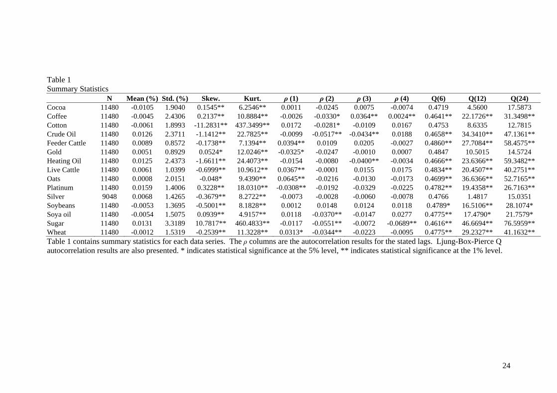
We present the summary statistics for each commodity series in Table 1. We examine the
distribution characteristics using the following statistics: mean, standard deviation,
skewness, kurtosis, and the autocorrelation characteristics using the Ljung-Box-Pierce (Q-
stats) test at lags of 6, 12 and 24 days, along with the estimated autocorrelation at lags of 1
to 4 days. Nine of the 15 commodity series have positive mean daily returns, with
Platinum has the largest mean daily return while Cocoa has the smallest. Sugar, Heating
Oil, and Coffee are the most volatile series. Statistically significant (at the 1% level)
skewness is prevalent in each commodity series. However, there is an almost even split
between positive (7 commodities) and negative skewness (8 commodites). Statistically
significant (at the 1% level) kurtosis is present in returns in all commodity series, which
indicates the presence of fat tails in each of the return distributions.
Turning to the time series properties of the samples, we observe that there is evidence of
positive (negative) autocorrelation at one lag in four (two) of the series. Negative
autocorrelation at two lags, three lags, and four lags is prevalent in six, two, and one of the
series respectively. However, the Ljung-Box test indicates that positive autocorrelation is
more prevalent at long lags.
11
[Insert Table 1 About Here]
3.2. Methodology
Tests of the profitability of technical trading rules in commodity futures markets (e.g.,
Stevenson and Bear, 1970) usually rely on the assumption that returns are stationary,
independent, and normally distributed. However, Lukac and Brorsen (1990) find that
technical trading returns on commodities are positively skewed and leptokurtic so these
tests may not be valid. We apply two more appropriate test procedures. The first is the
BLL (1992) bootstrapping methodology, while the second is the Reality Check
bootstrapping technique of STW (1999) that accounts for data-snooping bias. We describe
each of these tests in more detail below.
We begin by applying the bootstrap methodology that BLL (1992) adopted. We fit a null
model to that data and generate the parameters of this model. We then randomly resample
the residuals 500 times. We use each series of resampled residuals and the model
parameters to generate random price series which have the same times-series properties as
the original series. Earlier work (e.g. BLL, 1992) shows that bootstrap results are invariant
to the choice of null model so we follow the established precedent in the literature (e.g.
Kwon and Kish, 2002) and focus on the GARCH-M null model. The GARCH-M model
we apply is presented in equations 1 to 3 (see BLL, 1992 for a detailed description of this
model):
rt = α + γσt2 + βεt-1 + εt (1)
σt2 = α0 + α1εt-1
2 + βσt-12 (2)
εt = σt zt zt ~ N(0,1) (3)
12
The BLL (1992) bootstrap methodology involves comparing the conditional buy and sell
returns generated by a trading rule on the original commodity series with the conditional
buy or sell returns generated from the same trading rule on a random simulated series. We
follow BLL (1992) and define the buy (sell) return as the mean return per period for all the
periods where the rule is long (short). The difference between the two means is the buy-sell
return. The proportion of times the buy-sell profit for the rule is greater on the 500 random
series than the original series is the buy-sell p-value. If, for a given rule, 24 of the 500
random series have a buy-sell profit greater than that on the original series the p-value will
be 0.048.
Our second test of profitability is the so-called While Reality Check bootstrap, introduced
by White (2000). This bootstrap-based test evaluates whether the profitability of the best
trading rule is statistically significant after adjusting for data-snooping bias which is
introduced by selecting the rule from a wide universe of rules. When there is a large
universe of rules some will be profitable due to randomness so explicitly adjusting for
data-snooping is critical. The White Reality Check accounts for this by adjusting down the
statistical significance of profitable trading rules if they are drawn from a large universe of
unprofitable rules. This is in contrast to the BLL (1992) approach where each rule is
evaluated in isolation.
Specifically, we follow STW (1999), and let ),...,1(, Mkf tk = be the period t return from
the k-th trading rule (out of a universe of M rules), relative to the benchmark (which is the
commodity return at time t). The performance statistic of interest is the mean period
relative return from the k-th rule, ∑ ==
T
t tkk Tff1 , / , where T is the number of periods in the
sample.
13
Like STW (1999), our null hypothesis is that the performance of the best trading rule,
drawn from the universe of M rules, is no better than the benchmark performance, i.e.,
0max:,...,10 ≤
= kMkfH
STW (1999) then use the stationary bootstrap of Politis and Romano (1994) on the M
values of kf to test the null hypothesis.3 To do this, each time-series of relative returns,
),...,1( Mkfk = , is resampled (with replacement) B times, i.e., for each of the M rules, we
resample the time-series of relative returns B times. Note that for each of the M rules, the
same B bootstrapped time-series are used. Following STW (1999), we set B = 500. For the
k-th rule, this generates B means, which we denote ),...,1(, Bbf bk =∗ , from the B resampled
time-series, where
),...,1(,/1
*,,, BbTff
T
tbtkbk ==∑
=
∗ .
The test two statistics employed in the test are:
][max,...,1 kMkM fTV
==
and
).,...,1(,)]([max *,,...,1
*, BbffTV kbkMkbM =−=
=
To generate the test statistic, MV is compared to the quantiles of the *,bMV distribution, i.e.,
we compare the maximum mean relative return from the M rules run on the original series,
3 We refer the reader to Appendix C of STW (1999) for the details. As per STW (1999), we set the probability parameter to 0.1.
(4)
(5)
(6)
(7)
14
with the maximum mean across the M rules from each of the 500 bootstraps. In this way,
the test evaluates the performance of the best rule with reference to the performance of the
whole universe. In the context of our analysis, the White Reality Check bootstrap test
allows us to compute a data-snooping adjusted p-value for the best rule in each of the file
rule families, in relation to the universe of 7,846 rules from which they are drawn.
4. Results
Our results provide strong evidence that the large universe of technical trading rules we
consider are not profitable when applied to 14 of the 15 commodity futures contracts we
examine. There is evidence that certain rules generate profits, but the statistical
significance of these profits disappears once data snooping bias is accounted for. We find
the best Moving Average trading rule generates profits on the Oats series that are
statistically significant after data snooping bias has been accounted for. These profits are
in excess of reasonable estimates of transactions costs. However, this profitability is not
evident in data for the 1995 – 2005 sub-period. Overall, we conclude that while we cannot
rule out the possibility that technical trading rules add value by complimenting some other
commodity trading strategy we can conclude that they do not consistently add value in
their own right.
Table 2 contains bootstrap results for the entire 1984 – 2005 period (with the exception of
Silver which starts in 1988). The p-value count columns document the number of rules that
are statistically significant out of the total universe of 7,846 rules. For rule to be
statistically significant at the 1% (5%) level, there would have to be 5 (25) or fewer
instances of the rule generating more profit on bootstrapped series than the original series.
15
The remaining columns contain results relating to the STW (1999) bootstrap technique.
The nominal p-value is the Reality Check p-value for the best rule, unadjusted for data-
snooping. The STW (1999) p-value is the data-snooping adjusted p-value, after accounting
for the fact the rule is drawn from a wider universe of 7,846 rules. The remaining columns
contain other results relating to the best trading rule for each commodity series.
It is clear that from the BLL (1992) results that there is at least one rule that generates
statistically significant on each of the fifteen commodity series. Coffee and Cotton have
the fewest rules generating statistically significant profits at the 5% level while Live Cattle
has the most. The pre-data snooping adjustment results for the STW (1999) bootstrapping
procedure are similar to their BLL (1992) counterparts for eight commodities in that there
is evidence of the best performing rule being statistically significant at the 5% level. For
the remaining eight commodity series there is no evidence of even the best performing rule
generating statistically significant profits at the 5% level. Despite these differences across
the two alternative bootstrapping techniques prior to data snooping, the results are very
clear once data snooping bias is accounted for.
[Insert Table 2 About Here]
After adjustment for data snooping bias the statistical significance of the best performing
rule on each of the series other than Oats disappears. The difference between the nominal
and STW (1999) p-values is considerable for each commodity (other than Oats) which
gives an indication of the size of the potential data snooping problem. Anyone testing a
few rules in isolation could incorrectly conclude that technical analysis does have value,
when it fact any profitability can be attributed to data snooping bias.
16
The best performing trading rule on the Oats series is the Moving Average rule involving
price and a two-day moving average of price. This rule generates statistically significant
(at the 1% level) profits after data snooping bias has been accounted for. These profits also
appear to be economically significant. Even though the trading rule generates many
trading signals (average days per trade is only 2.85), the average return per trade is
0.403%. This suggests that profits are available after transactions costs even if we assume
that one-way transaction costs are at the upper extreme of the Locke and Venkatesh (1997)
estimated range of 0.0004% to 0.033%. The proportion of winning trades to total trades
for oats (41%) indicates that technical trading rules can generate profits overall even if
more losing than winning trades are generated.
No one rule performs best on each of the commodity series. Rather, rules form each of the
rule families are represented across each of the 15 series. While the short-term Moving
Average rule generates the largest profits for the Oats series, a relatively long-term Support
and Resistance rule generates the largest profits on the Gold series. This rule only signals
4 trades, or which all are profitable. It generates an average return per trade of 34.9% but
this is not statistically significant (either before or after data snooping adjustment) as the
average daily return is only 0.024%.
We consider the robustness of these results by breaking each data series in half. Table 3
contains bootstrap results for the 1984 – 1994 period (except for silver which is 1998 –
1996). Given this consistency between the BLL (1992) and STW (1999) bootstrap results
for the entire period we only present the more common STW (1999) results. The nominal
p-value results indicate that, on average, the best performing rule on commodity series is
more statistically significant in the early period than the entire period. Nine of the 15
17
nominal p-values are lower (more statistically significant) in the 1984 – 1994 period.
Similarly, the average daily return is higher for the best rules on 10 of the 15 series in the
early period.
Despite the evidence of more profitability to trading rules in the earlier period, the overall
conclusions about their profitability made earlier still stand. There is strong evidence that
the best performing trading rule generates statistically significant profits in the majority of
series before data snooping is accounted for, but this profitability disappears in all but the
Oats series once data snooping bias is adjusted for. The Moving Average rule involving
price and a two-day moving average of price is again the most profitable rule on the Oats
series. The proportion of all trades that turn out to be winning trades is similar (41%) to
the entire series, while the average return per trade is slightly higher (0.473%).
[Insert Table 3 About Here]
Results for the second sub-period (1995 – 2005, except for silver which is 1989 – 2005)
are presented in Table 4. Consistent with the entire period and first sub-period results,
there is no evidence that the best performing trading rule produces profits that are
statistically significant once data snooping bias is adjusted for the majority of commodity
series. This also applies to Oats, which was previously able to be traded profitably using a
short-term Moving Average rule. The fact that the best performing rule on the Oats series
in this period is a Filter Rule and even this is not profitable after data snooping adjustment
indicates that profitability of the Moving Average rule is not robust to different sub-
periods.

18
Similar to Gold in the entire period, the best performing rule on Heating Oil in the second
sub-period generates profits in excess of 30% per trade. Despite the large size of these
profits, they are not statistically significant before or after data snooping adjustment due to
the small number of trades generated (7) and the corresponding low average return per day.
A comparison of the average return per trade figures for the first and second sub-periods
indicates there is some evidence of a decline in profitability over time. Nine of the 15
commodity series have a best rule which yield lower profits in the second period.
[Insert Table 4 About Here]
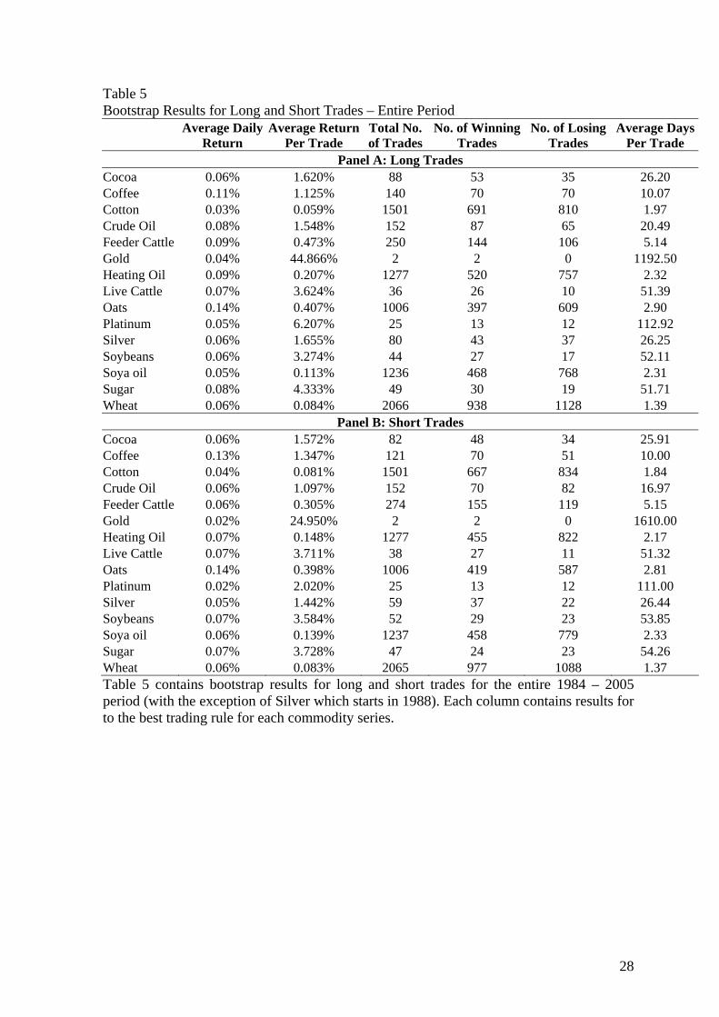
We complete our analysis by considering whether there are major differences between the
profits generated by the long and short signals generated by the best trading rule for the
entire period.4 It is possible that a rule generates particularly profitable long (short) signals
but the lack of profitability in short (long) signals offsets this profitability. If this is the
case then an investor may choose to act on the long (short) signals but ignore the short
(long) signals.
The results presented in Table 5 indicate there is some evidence that the average daily
return is higher for long trades than short trades. This is evident in 11 of the 15 commodity
series. This is unsurprising as while commodity futures, as measured by the Reuters-CRB
index, experienced considerable volatility over the 1984 - 2005 period we study, they did
increase 27%. This indicates that, on average, there was more upward than downward
movement. Although there is evidence of superior performance for long trades, the
difference between the profits generated by long and short trades is generally small. The
4 Equivalent results for each sub-period are very similar so are not reported in order to conserve space. The interested reader should contact the authors for these results.
19
differences in average daily return per day are all 0.03% or less, which suggests an investor
applying these technical trading rules is unlikely to be able to consistently add meaningful
incremental profit by following the long signals of a rule and ignoring the short signals.
[Insert Table 5 About Here]
In summary, our results demonstrate that technical trading rules cannot be used to
profitably trade the 15 commodity series we consider. While there is evidence of the best
performing rule on the oats series generating profits that are statistically significant after
data snooping adjustment and economically significant over the entire 1984 – 2005 period,
this rule is not profitable in the more recent 1995 – 2005 sub-period. The majority of
commodity series have a trading rule that generates profitable trades but the statistical
significance of this profitability disappears once data snooping bias is accounted for.
5. Conclusions
We re-consider whether quantitative trading rules can be profitably applied to commodity
futures trading. Compared to previous work, we study a larger universe of technical
trading rules, focus on more recent data and address the issue of data snooping bias using
robust statistical techniques. Commodity futures have been trading for long time, but it is
only recently that debate has begun about the merits of including commodity futures in
mainstream portfolios. Recent work has shown commodities can be very effective at
providing diversification for both stock and bond portfolios, which may be due to their
20
strong performance in periods of unexpected inflation or due to safe haven qualities of
precious metal commodities.
Futures markets have several features that make them a more attractive market for active
trading strategies than stock markets. In particular, transaction costs are lower and it is
easier to short-sell. It is therefore interesting that recent studies have shown that
commodity futures can be successfully traded with a variety of strategies, including using
information on market positions from the Commodity Futures Trading Commission,
medium-term momentum strategies and short-term contrarian strategies.
We extend this literature by considering 7,846 trading rule specifications from five rule
families (Filter Rules, Moving Average Rules, Support and Resistance Rules, Channel
Breakouts, and On Balance Volume Rules). We apply these rules to the 15 major
commodity series over the 1/1/1984 – 31/12/2005 period. We study the entire series and
two equal sub-periods. Unlike the previous commodity futures technical analysis
literature, we apply a suite of tests to test the statistically significance of the trading rules
profits. These are the Brock, Lakonishok and LeBaron (1992) approach of fitting null
models to the data, generating random series and comparing the results from running the
rules on the original series to those from running on the randomly generated bootstrapped
series, and bootstrapping technique of Sullivan, Timmerman, and White (1999) which
adjusts for data snooping bias.
We find that the best trading rule for each commodity series typically produces profits that
are statistically significant at the 5% level. However, the trading rules we consider do not
generate profits on 14 of the 15 commodity series after an adjustment is made for data

21
snooping bias. This underscores the importance of conducting a robust adjustment for data
snooping bias. A short-term moving average rule generates statistically significant profits
(after data snooping bias adjustment) for the Oats series. This profitability appears to be in
excess of reasonable estimates of transactions costs, however it is not robust to our sub-
period analysis. Rather, the profitability disappears in the most recent sub-period. While
we cannot rule out the possibility that technical trading rules can compliment some other
trading strategy, we do conclusively show that they are not profitable when used in
isolation, despite their wide following.
22
References
Basu, D., Oomen, R., Stremmer, A., 2006. How to time the commodity market. Working
paper, Warwick Business School. Bessembinder, H., 1992. Systematic risk, hedging pressure and risk premiums in futures
markets. Review of Financial Studies 5, 637--667. Bessembinder, H., Chan, K., 1998. Market efficiency and the returns to technical analysis.
Financial Management, 272, 5--13. Brock, W., Lakonishok, J., LeBaron, B., 1992. Simple technical trading rules and the
stochastic properties of stock returns. Journal of Finance, 485, 1731--1764. Donchian, R. D. 1960. High finance in copper. Financial Analysts Journal, Nov/Dec. 133--
142. Engle, R.H, Lilien, D., Robins, R.P. 1987. Estimating time varying risk premia in the term
structure: The ARCH-M model. Econometrica, 55, 391--407. Erb, C., Harvey, C., 2006. The strategic and tactical value of commodity futures. Financial
Analysts Journal 62, 2, 69--97. Gorton, G., Rouwenhorst, K., 2006. Facts and fantasies about commodity futures,
Financial Analysts Journal 622, 47--68. Hiller, D., Draper, P., Faff, R., 2006. So precious metals shine? An investment perspective.
Financial Analysts Journal 62, 2, 98--106. Irwin, S.H., Zulauf, C.R., Gerlow, M.E, Tinker, J.N., 1997. A performance comparison of
a technical trading system with ARIMA models for soybean complex prices.” Advances in Investment Analysis and Portfolio Management 4,193--203.
Jegadeesh, N., Titman, S. 1993. Returns to buying winners and selling losers: Implications
for stock market efficiency. Journal of Finance 48, 65--91. Kwon, K.Y, Kish, R.J. 2002. A comparative study of technical trading strategies and return
predictability: An extension of Brock, Lakonishok, and LeBaron 1992 using NYSE and NASDAQ indices. Quarterly Review of Economics and Finance 423, 611--631.
Lehmann, B. 1990. Fads, martingales, and market efficiency. Quarterly Journal of
Economics 105, 1--28. Lesmond, D.A., Ogden, J.P., Trzcinka, C.A. 1999. A new estimate of transactions costs.
Review of Financial Studies 125, 1113--1141. Lesmond, D. A., Schill, M.J., Zhou, C., 2004. The illusory nature of momentum profits,
Journal of Financial Economics 71, 349--380.
23
Lo, A. W., MacKinlay, A.C. 1990. When are contrian profits due to stock market overreaction? Review of Financial Studies 3, 175--208.
Locke, P.R., Venkatesh, P.C., 1997. Futures market transactions costs. Journal of Futures
Markets 172, 229--245. Lui, Y., Mole, D., 1998. The use of fundamental and technical analysis by foreign
exchange dealers: Hong Kong evidence. Journal of International Money and Finance 17; 535--545.
Lukac, L.P., Brorsen, B.W., 1990. A comprehensive test of futures market disequilibrium.
The Financial Review, 244, 593--614. Lukac, L.P., Brorsen, B.W., Irwin, S.H., 1988. A test of futures market disequilibrium
using twelve different technical trading systems. Applied Economics 20, 623--539. Miffre, J., Rallis, G., 2007. Momentum strategies in commodity futures markets. Journal of
Banking and Finance – forthcoming. Oberlechner, T., 2001. Importance of technical and fundamental analysis in the European
foreign exchange market. International Journal of Finance and Economics 6; 81--93.
Olson, D., 2004. Have trading rule profits in the currency markets declined over time?
Journal of Banking and Finance 28, 85--105. Park, C-H., Irwin, S.H., 2004. The profitability of technical analysis: A review. AgMAS
Research Report. Politis, D., Romano, J., 1994. The stationary bootstrap. Journal of American Statistical
Association 89; 1303--1313. Stevenson, R. A., Bear, R. M., 1970. Commodity Futures: Trends or Random Walks?
Journal of Finance 25, 65--81. Sullivan, R., Timmermann, A., White, H., 1999. Data-snooping, technical trading rule
performance, and the bootstrap. Journal of Finance 245, 1647--1691. Vrugt, Evert B., Bauer, R., Molenaar, R., & Steenkamp, T., 2004. Dynamic commodity
trading strategies. Working paper, July. Wang, C., Yu, M., 2004. Trading activity and price reversals in futures markets. Journal of
Banking and Finance 28, 1337--1361. White, H., 2000. A reality check for data snooping. Economterica 685 1097--1126.
24
Table 1 Summary Statistics N Mean (%) Std. (%) Skew. Kurt. ρ (1) ρ (2) ρ (3) ρ (4) Q(6) Q(12) Q(24) Cocoa 11480 -0.0105 1.9040 0.1545** 6.2546** 0.0011 -0.0245 0.0075 -0.0074 0.4719 4.5600 17.5873 Coffee 11480 -0.0045 2.4306 0.2137** 10.8884** -0.0026 -0.0330* 0.0364** 0.0024** 0.4641** 22.1726** 31.3498** Cotton 11480 -0.0061 1.8993 -11.2831** 437.3499** 0.0172 -0.0281* -0.0109 0.0167 0.4753 8.6335 12.7815 Crude Oil 11480 0.0126 2.3711 -1.1412** 22.7825** -0.0099 -0.0517** -0.0434** 0.0188 0.4658** 34.3410** 47.1361** Feeder Cattle 11480 0.0089 0.8572 -0.1738** 7.1394** 0.0394** 0.0109 0.0205 -0.0027 0.4860** 27.7084** 58.4575** Gold 11480 0.0051 0.8929 0.0524* 12.0246** -0.0325* -0.0247 -0.0010 0.0007 0.4847 10.5015 14.5724 Heating Oil 11480 0.0125 2.4373 -1.6611** 24.4073** -0.0154 -0.0080 -0.0400** -0.0034 0.4666** 23.6366** 59.3482** Live Cattle 11480 0.0061 1.0399 -0.6999** 10.9612** 0.0367** -0.0001 0.0155 0.0175 0.4834** 20.4507** 40.2751** Oats 11480 0.0008 2.0151 -0.048* 9.4390** 0.0645** -0.0216 -0.0130 -0.0173 0.4699** 36.6366** 52.7165** Platinum 11480 0.0159 1.4006 0.3228** 18.0310** -0.0308** -0.0192 -0.0329 -0.0225 0.4782** 19.4358** 26.7163** Silver 9048 0.0068 1.4265 -0.3679** 8.2722** -0.0073 -0.0028 -0.0060 -0.0078 0.4766 1.4817 15.0351 Soybeans 11480 -0.0053 1.3695 -0.5001** 8.1828** 0.0012 0.0148 0.0124 0.0118 0.4789* 16.5106** 28.1074* Soya oil 11480 -0.0054 1.5075 0.0939** 4.9157** 0.0118 -0.0370** -0.0147 0.0277 0.4775** 17.4790* 21.7579* Sugar 11480 0.0131 3.3189 10.7817** 460.4833** -0.0117 -0.0551** -0.0072 -0.0689** 0.4616** 46.6694** 76.5959** Wheat 11480 -0.0012 1.5319 -0.2539** 11.3228** 0.0313* -0.0344** -0.0223 -0.0095 0.4775** 29.2327** 41.1632** Table 1 contains summary statistics for each data series. The ρ columns are the autocorrelation results for the stated lags. Ljung-Box-Pierce Q autocorrelation results are also presented. * indicates statistical significance at the 5% level, ** indicates statistical significance at the 1% level.

25
Table 2 Bootstrap Results – Full Period
BLL p-Value Count (1%)
BLL p-Value Count (5%)
Nominal p-Value
STW p-Value
Average Daily Return
Average Return Per Trade
Total No. of Trades
No. of Winning Trades
No. of Losing Trades
Average Days Per Trade
Cocoa 13 111 0.032 0.628 0.047% 1.597% 170 101 69 26.06 Coffee 4 82 0.052 0.670 0.056% 1.228% 261 140 121 10.04 Cotton 26 129 0.054 0.532 0.037% 0.070% 3002 1358 1644 1.91 Crude Oil 51 193 0.068 0.784 0.070% 1.323% 304 157 147 18.73 Feeder Cattle 93 311 0.038 0.676 0.035% 0.385% 524 299 225 5.14 Gold 77 262 0.106 0.832 0.024% 34.908% 4 4 0 1401.25 Heating Oil 27 137 0.038 0.740 0.079% 0.178% 2554 975 1579 2.25 Live Cattle 325 573 0.006 0.428 0.047% 3.668% 74 53 21 51.35 Oats 77 253 0.000 0.010 0.141% 0.403% 2012 816 1196 2.85 Platinum 10 132 0.190 0.932 0.036% 4.113% 50 26 24 111.96 Silver 26 128 0.068 0.754 0.048% 1.565% 139 80 59 26.33 Soybeans 46 179 0.008 0.248 0.058% 3.442% 96 56 40 53.05 Soya oil 14 115 0.016 0.372 0.055% 0.126% 2473 926 1547 2.32 Sugar 13 100 0.132 0.806 0.068% 4.037% 96 54 42 52.96 Wheat 64 121 0.008 0.310 0.060% 0.084% 4131 1915 2216 1.38 Table 2 contains bootstrap results for the entire 1984 – 2005 period (with the exception of Silver which starts in 1988). The p-value count columns document the number of rules that are statistically significant out of the total universe of 7,846 rules. For rule to be statistically significant at the 1% (5%) level, there would have to be 5 (25) or fewer instances of the rule generating more profit on bootstrapped series than the original series. The remaining columns contain results relating to the Sullivan, Timmerman, and White (1999) (STW) bootstrap technique. The nominal p-value is the Reality Check p-value for the best rule, unadjusted for data-snooping. The STW (1999) p-value is the data-snooping adjusted p-value, after accounting for the fact the rule is drawn from a wider universe of 7,846 rules. The remaining columns contain results relating to the best trading rule for each commodity series.

26
Table 3 Bootstrap Results – First Sub-Period
Nominal p-Value
STW p-Value
Average DailyReturn
Average Return Per Trade
Total No. of Trades
No. of Winning Trades
No. of Losing Trades
Average Days Per Trade
Cocoa 0.012 0.486 0.070% 5.030% 40 26 14 50.00 Coffee 0.052 0.720 0.080% 7.676% 30 19 11 50.27 Cotton 0.066 0.466 0.063% 4.867% 37 21 16 74.92 Crude Oil 0.012 0.448 0.113% 2.234% 145 72 73 19.48 Feeder Cattle 0.052 0.742 0.035% 5.908% 17 11 6 165.12 Gold 0.044 0.716 0.034% 0.303% 320 165 155 8.93 Heating Oil 0.038 0.680 0.084% 0.188% 1282 488 794 2.24 Live Cattle 0.032 0.610 0.044% 0.507% 249 156 93 5.08 Oats 0.000 0.016 0.172% 0.473% 1045 433 612 2.75 Platinum 0.066 0.728 0.053% 3.720% 41 24 17 68.24 Silver 0.032 0.674 0.003% 1.415% 4 3 1 493.75 Soybeans 0.014 0.320 0.054% 5.337% 29 20 9 92.76 Soya oil 0.026 0.680 0.055% 26.076% 6 5 1 477.67 Sugar 0.082 0.854 0.119% 7.136% 48 28 20 52.50 Wheat 0.022 0.456 0.078% 0.189% 1187 459 728 2.42 Table 3 contains bootstrap results for the 1984 – 1994 period (except for silver which is 1988 – 1996). Each column contains results relating to the Sullivan, Timmerman, and White (1999) (STW) bootstrap technique. The nominal p-value is the Reality Check p-value for the best rule, unadjusted for data-snooping. The STW (1999) p-value is the data-snooping adjusted p-value, after accounting for the fact the rule is drawn from a wider universe of 7,846 rules. The remaining columns contain results relating to the best trading rule for each commodity series.

27
Table 4 Bootstrap Results – Second Sub-Period
Nominal p-Value
STW p-Value
Average Daily Return
Average Return Per Trade
Total No. of Trades
No. of Winning Trades
No. of Losing Trades
Average Days Per Trade
Cocoa 0.060 0.774 0.065% 1.211% 153 81 72 10.32 Coffee 0.022 0.434 0.130% 4.089% 91 57 34 27.15 Cotton 0.022 0.444 0.079% 2.622% 86 53 33 27.03 Crude Oil 0.118 0.970 0.079% 0.822% 276 102 174 10.38 Feeder Cattle 0.036 0.782 0.025% 7.068% 10 4 6 266.80 Gold 0.084 0.772 0.041% 1.325% 88 56 32 27.68 Heating Oil 0.186 0.932 0.082% 33.498% 7 6 1 373.71 Live Cattle 0.028 0.674 0.053% 4.506% 34 29 5 50.00 Oats 0.020 0.528 0.114% 0.151% 2160 958 1202 1.31 Platinum 0.346 0.984 0.043% 3.393% 36 17 19 75.42 Silver 0.072 0.822 0.081% 2.558% 74 47 27 25.14 Soybeans 0.050 0.660 0.062% 3.724% 48 29 19 54.60 Soya oil 0.014 0.274 0.078% 0.188% 1179 472 707 2.43 Sugar 0.010 0.554 0.102% 9.474% 31 16 15 88.10 Wheat 0.000 0.212 0.108% 0.143% 2163 1058 1105 1.31 Table 4 contains bootstrap results for the 1995 – 2005 period (except for silver which is 1997 – 2005). Each column contains results relating to the Sullivan, Timmerman, and White (1999) (STW) bootstrap technique. The nominal p-value is the Reality Check p-value for the best rule, unadjusted for data-snooping. The STW (1999) p-value is the data-snooping adjusted p-value, after accounting for the fact the rule is drawn from a wider universe of 7,846 rules. The remaining columns contain results relating to the best trading rule for each commodity series.
28
Table 5 Bootstrap Results for Long and Short Trades – Entire Period
Average Daily
Return Average Return
Per Trade Total No. of Trades
No. of Winning Trades
No. of Losing Trades
Average Days Per Trade
Panel A: Long Trades Cocoa 0.06% 1.620% 88 53 35 26.20 Coffee 0.11% 1.125% 140 70 70 10.07 Cotton 0.03% 0.059% 1501 691 810 1.97 Crude Oil 0.08% 1.548% 152 87 65 20.49 Feeder Cattle 0.09% 0.473% 250 144 106 5.14 Gold 0.04% 44.866% 2 2 0 1192.50 Heating Oil 0.09% 0.207% 1277 520 757 2.32 Live Cattle 0.07% 3.624% 36 26 10 51.39 Oats 0.14% 0.407% 1006 397 609 2.90 Platinum 0.05% 6.207% 25 13 12 112.92 Silver 0.06% 1.655% 80 43 37 26.25 Soybeans 0.06% 3.274% 44 27 17 52.11 Soya oil 0.05% 0.113% 1236 468 768 2.31 Sugar 0.08% 4.333% 49 30 19 51.71 Wheat 0.06% 0.084% 2066 938 1128 1.39
Panel B: Short Trades Cocoa 0.06% 1.572% 82 48 34 25.91 Coffee 0.13% 1.347% 121 70 51 10.00 Cotton 0.04% 0.081% 1501 667 834 1.84 Crude Oil 0.06% 1.097% 152 70 82 16.97 Feeder Cattle 0.06% 0.305% 274 155 119 5.15 Gold 0.02% 24.950% 2 2 0 1610.00 Heating Oil 0.07% 0.148% 1277 455 822 2.17 Live Cattle 0.07% 3.711% 38 27 11 51.32 Oats 0.14% 0.398% 1006 419 587 2.81 Platinum 0.02% 2.020% 25 13 12 111.00 Silver 0.05% 1.442% 59 37 22 26.44 Soybeans 0.07% 3.584% 52 29 23 53.85 Soya oil 0.06% 0.139% 1237 458 779 2.33 Sugar 0.07% 3.728% 47 24 23 54.26 Wheat 0.06% 0.083% 2065 977 1088 1.37 Table 5 contains bootstrap results for long and short trades for the entire 1984 – 2005 period (with the exception of Silver which starts in 1988). Each column contains results for to the best trading rule for each commodity series.