Joint Feature-Sample Selection and Robust Diagnosis ofParkinson’s Disease from MRI Data

Ehsan Adelia, Feng Shia, Le Ana, Chong-Yaw Weea,b, Guorong Wua, Tao Wanga,c,d,Dinggang Shena,e,∗

aDepartment of Radiology and BRIC, University of North Carolina-Chapel Hill, NC, 27599, USAbDepartment of Biomedical Engineering, National University of Singapore, Singapore

cDepartment of Geriatric Psychiatry, Shanghai Mental Health Center, Shanghai Jiao Tong UniversitySchool of Medicine, Shanghai, China

dAlzheimer’s Disease and Related Disorders Center, Shanghai Jiao Tong University, Shanghai, ChinaeDepartment of Brain and Cognitive Engineering, Korea University, Seoul 02841, Republic of Korea

Abstract

Parkinson’s disease (PD) is an overwhelming neurodegenerative disorder caused by

deterioration of a neurotransmitter, known as dopamine. Lack of this chemical mes-

senger impairs several brain regions and yields various motor and non-motor symp-

toms. Incidence of PD is predicted to double in the next two decades, which urges

more research to focus on its early diagnosis and treatment. In this paper, we propose

an approach to diagnose PD using magnetic resonance imaging (MRI) data. Specif-

ically, we first introduce a joint feature-sample selection (JFSS) method for selecting

an optimal subset of samples and features, to learn a reliable diagnosis model. The

proposed JFSS model effectively discards poor samples and irrelevant features. As a

result, the selected features play an important role in PD characterization, which will

help identify the most relevant and critical imaging biomarkers for PD. Then, a robust

classification framework is proposed to simultaneously de-noise the selected subset of

features and samples, and learn a classification model. Our model can also de-noise

testing samples based on the cleaned training data. Unlike many previous works that

perform de-noising in an unsupervised manner, we perform supervised de-noising for

both training and testing data, thus boosting the diagnostic accuracy. Experimental

results on both synthetic and publicly available PD datasets show promising results.

∗Corresponding authorEmail address: dgshen@med.unc.edu (Dinggang Shen)

Preprint submitted to NeuroImage June 28, 2016

To evaluate the proposed method, we use the popular Parkinson’s progression markers

initiative (PPMI) database. Our results indicate that the proposed method can differ-

entiate between PD and normal control (NC), and outperforms the competing methods

by a relatively large margin. It is noteworthy to mention that our proposed framework

can also be used for diagnosis of other brain disorders. To show this, we have also

conducted experiments on the widely-used ADNI database. The obtained results indi-

cate that our proposed method can identify the imaging biomarkers and diagnose the

disease with favorable accuracies compared to the baseline methods.

Keywords: Parkinson’s disease, diagnosis, sparse regression, joint feature-sample

selection, matrix completion, robust linear discriminant analysis.

1. Introduction

Diagnosis of neurodegenerative brain disorders using medical imaging is a chal-

lenging task due to different factors, including a wide variety of artifacts in the image

acquisition procedure, the imposed errors due to preprocessing, and the large amount

of intrinsic inter-subject variabilities. Among the neurodegenerative disorders, Parkin-5

son’s disease (PD) is one of the most common ones, with a high socioeconomic impact.

PD is provoked by progressive impairment and deterioration of brain neurons, caused

by a gradual halt in the production of a vital chemical messenger. PD symptoms start

to appear with the loss of these neurotransmitters in the brain, notably dopamine. The

neuropathology of PD is pinpointed by a selective loss of dopaminergic neurons in10

the substantia nigra (SN); nevertheless, in recent studies a widespread involvement of

other structures and tissues is widely researched [1]. The degeneration of dopaminer-

gic neurons results in decreased levels of dopamine in the putamen of the dorsolateral

striatum, leading to dysfunction of direct and indirect pathways of movement control

[2]. Furthermore, researchers have identified that it can also cause non-motor problems15

to the subjects (e.g., depression, anxiety, apathy/abulia, etc.) [3, 4]. People with PD

may lose up to 80% of dopamine before symptoms appear [1, 5, 6]. Thus, early diag-

nosis and treatment are of great interest and are crucial to detain progression of PD in

its initial stages.

2

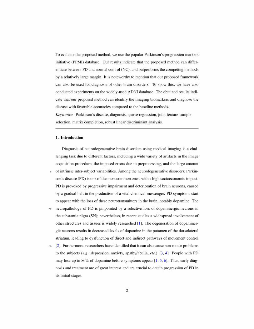
Figure 1: An illustration of the brain regions affected by PD in different stages of the disease. Darker blue

denotes the earlier and more severely affected regions.

Previous clinical studies [5] show that the disease is initiated in the brainstem and20

mid-brain regions; however, with time, it also affects many other brain regions. An

illustration of PD progression is shown in Figure 1, derived from the results achieved

by [5]. In this figure, darker regions are those affected earlier in the process of PD

progression.

Current diagnosis of PD mainly depends on the clinical symptoms. But, the dopamine25

transporter positron emission computed tomography is very expensive and cannot be

popularized on the clinical diagnosis of PD patients. Therefore, other neuro-imaging

techniques could be crucial pathways for PD early diagnosis. For example, SPECT

imaging is usually considered for the differential diagnosis of PD and often used for

people with tremor [7, 6]. PET is utilized for PD diagnosis [8], while MRI is often30

employed for the differential diagnosis of PD syndromes [6, 3, 9], as well as to analyze

the structural changes in PD patients [10] and their deferential diagnosis [11, 12].

Thus, through analyzing the deep and mid-brain regions, along with cortical sur-

faces, we could potentially identify the imaging biomarkers for PD. Accordingly, we

create a PD-specific atlas and further extract features by non-linearly registering this35

atlas to each subject’s brain image. The extracted features represent the tissue volumes

3

of each labeled ROI.

Recently, with the advances in the area of machine learning and data-driven anal-

ysis methodologies, significant amount of research efforts have been dedicated to di-

agnosis and progression prediction of neurodegenerative diseases using different brain40

imaging modalities [7, 13, 6, 14, 9]. Automatic PD diagnosis and progression pre-

diction could help physicians and patients avoid unnecessary medical examinations

or therapies, as well as potential side effects and safety risks [15]. Machine learning

and pattern recognition methods could simplify the development of these automatic

PD diagnosis approaches. For instance, Prashanth et al. [7] use intensity features ex-45

tracted from SPECT images along with an SVM classifier, while Focke et al. [11]

use the voxel-based morphometry (VBM) on T1-weighted MRI with an SVM clas-

sifier to identify idiopathic Parkinson syndrome patients. In another work, Salvatore

et al. [12] proposes a method based on principal component analysis (PCA) on mor-

phological T1-weighted MRI, in combination with an SVM for diagnosis of PD and50

progressive supranuclear palsy (PSP) patients. In the past several years, some research

has exploited MRI in order to analyze changes in different brain regions in PD patients

[6, 3, 10, 11, 12]. Along with the impairment of the dopamine production process,

many brain regions are also affected, leading to several movement problems and some-

times also a number of non-motor symptoms [5]. Literature studies show that these55

influences could be characterized by the information acquired from the MRI data [6].

In this paper, we use MR images to diagnose PD and analyze the imaging biomark-

ers. To this end, we extract features from predefined brain regions and analyze changes

and variations between PD and normal control (NC) subjects. In order to build a re-

liable system, we need to take several important issues into account. As mentioned60

earlier, the quality of MR images can be affected by different factors, e.g., patient

movements, radiations or device limitations. Most existing works manually discard

poor subject images, which could eventually induce undesirable bias to the learned

model. Therefore, it is of great interest to automatically select the most reliable sam-

ples, boosting up robustness of the method and its application under a clinical setting.65

On the other hand, many studies analyze MR images by parcellating them into sev-

eral pre-defined regions of interest (ROIs) and then extracting features from each ROI

4

[16, 17, 13]. It is noted that PD, like many other neurodegenerative diseases, highly

affects a number of brain regions [5]. Therefore, it is also desirable to select the most

important and relevant regions for our diagnosis procedure. This also leads to identi-70

fying the biomarkers for the disease, as well as initiating studies to the future clinical

analysis. Similar studies for identification of biomarkers for Alzheimer’s disease (AD)

are previously conducted in many works [13, 18, 19]. But, such studies are scarce for

PD, in the literature.

Considering all these factors, we seek to automatically select both a subset of the75

subjects and the most discriminative brain ROIs to construct a robust model for PD

diagnosis. Each subject will form a sample in our classification task. Samples are

described by the features extracted from their ROIs. In many previous works, either

feature selection [18, 19] or sample selection [20] was performed individually, or both

were considered sequentially [13]. We observe that these two processes (or two sub-80

problems) affect each other, and that performing one before the other does not guaran-

tee the selection of the best overall subsets for both features and samples. Thus, these

two sub-problems are overlapping, but do not have optimal sub-structures [21]. In

other words, optimal overall solution is not composed of optimal solution to each sub-

problem. This motivates us to jointly search for the best subsets for both features and85

samples. Specifically, in this paper, we introduce a novel joint feature-sample selection

(JFSS) method based on how well the training labels could be represented sparsely by

different numbers of features and samples. Then, we further introduce a robust classi-

fication scheme, specially designed to enhance the robustness to noise. The proposed

robust classification framework follows the least-squares linear discriminant analysis90

(LS-LDA) [22] formulation and the robust regression scheme [23].

Many previous researches have been conducted on feature and sample selection

[13, 24, 25, 26]. But, few of them consider a joint formulation [27]. Authors in [27]

extend the classic relevance vector machine (RVM) formulation by adding two parame-

ter sets for feature and sample selection in a Bayesian graphical inference model. They95

consider sparsity in both feature and sample domains, as we do, but instead they solve

the problem in a marginal likelihood maximization procedure. In contrast, we develop

a single optimization problem for jointly selecting features and samples. Our formu-

5

MRI

...

Segmention

...

Brain Parcellation

...

Atla

s

· · ·

· · ·

· · ·

...· · ·

Feature Vectors(WM, GM, CSF) x11 x12 x13 . . . x1d

x21 x22 x23 . . . x2dx31 x32 x33 . . . x3d

......

.... . .

...xN1 xN2 xN3 . . . xNd

X ∈ RN×d

y1y2y3

...yN

y ∈ RN

x11 x12 . . . x1dx21 x22 . . . x2d

......

. . ....

xN1 xN2 . . . xNd

X ∈ RN×d

y1y2...yN

y ∈ RN

JFSS

De-noising ...

= ...

+

−×−−−××−−−−−...−−×−×−

X D E

Classifying using the cleaned data matrix D and y.

RL

DA

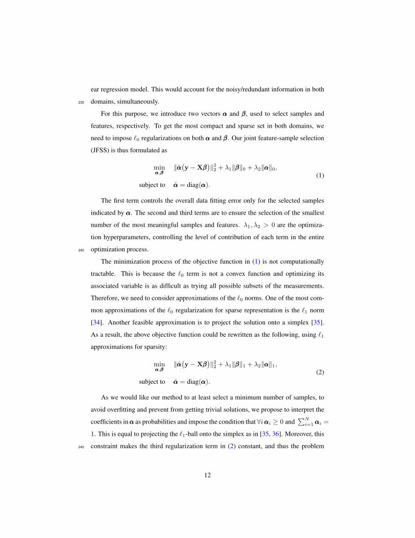
Figure 2: Overview of our proposed method. First, the MR images are processed and tissue-segmented.

Then, the anatomical automatic labeling (AAL) atlas is non-linearly registered to each subject’s original MR

image, and then the WM, GM and CSF volumes of each ROI are calculated as features. These features form

X, and the corresponding labels form y. Through our proposed joint feature-sample selection (JFSS), we

discard some uninformative features and samples, leading to X and y. Then, we train a robust classifier

(i.e., Robust LDA), in which we jointly decompose X into cleaned data D and its noise component E, and

classify the cleaned data.

lation is reduced to two simple and convex problems and therefore can be efficiently

solved.100

Figure 2 illustrates an overview of our proposed method. After preprocessing the

subjects’ MRI scans, we extract features from their pre-defined brain ROIs, and select

the best subsets of features and samples through our proposed JFSS. The joint feature-

sample selection procedure is able to simultaneously discard irrelevant samples and

redundant features. After JFSS, there may still be some random noise in the remaining105

data. To further clean the data, we decompose it into two parts, cleaned data and its

noise component. This is done in conjugation with the classification process, in a

supervised manner, to increase the classification robustness to noise. Additionally, the

testing data is also de-noised through representing the data as a locally compact linear

6

combination of the cleaned training data.110

The key methodological contributions in our work are multi-fold: (1) We propose

a new joint feature-sample selection (JFSS) procedure, which jointly selects the best

subset of most discriminative features and best samples to build a classification model.

(2) We utilize the robust regression method in [23] and further develop a robust clas-

sification model. In addition, we propose to de-noise the testing data based on the115

supervised cleaned training samples. (3) We apply our method for PD diagnosis, as

the diagnosis methods for PD are scarce. (4) In order to extract useful features for PD

diagnosis, we specifically define some new clinically-relevant ROIs for PD. Therefore,

finally the automated data-driven methods can be developed for PD diagnosis or further

analyses.120

2. Data acquisition and preprocessing

The data used in this paper was obtained from the Parkinson’s progression markers

initiative (PPMI) database1 [28]. PPMI is the first substantial study for identifying

PD progression markers to advance the overall understanding of the disease. PPMI is

an international study with multiple centers around the world designated to identify the125

progression of PD markers, to enhance the understanding of the disease, and to provide

crucial tools for succeeding in PD modifying therapeutic trials. They seek to establish

standardized protocols for acquisition, transfer and analysis of clinical, imaging and

biospecimen data, and investigate novel methods that demonstrate interval changes in

PD patients, compared to normal controls. All these could be used by the PD research130

community to elevate knowledge about the disease and an understanding of how to

cure or slow down its progression.

PD subjects in the PPMI study are de novo PD patients, newly diagnosed and un-

medicated. The healthy/normal control subjects are both age- and gender-matched with

the PD subjects. The subjects and their stagings are evaluated using the widely used135

Hoehn and Yahr (H&Y) scale [29]. H&Y scale defines board categories, which rate

1http://www.ppmi-info.org/data

7

the motor function for PD patients. H&Y stages correlate with motor decline, neu-

roimaging studies of dopaminergic loss and deterioration in quality of life [30]. The

original version has a 5-point scale (Stages 1-5) measurement. Most of the studies in

PD evaluated disease progression through analyzing patients and the time taken for140

them to reach one of the H&Y stages. The subjects in the first stage have unilateral

involvement only, often with the least or no functional impairment. They have mild

symptoms, which are inconvenient but not disabling. The second stage has bilateral

or midline involvements, but still with no impairment of balance. For these subjects,

the posture and gait are usually affected. Stage three shows the first signs of impaired145

reflexes. The patient will show significant slowing of the body movements and mod-

erately severe dysfunction. In the fourth stage, the disease is fully developed and is

severely disabling; the patient can still walk but to a limited extent, and might not be

able to live alone any longer. In the fifth (final) stage, the patient will have a confine-

ment to bed or will be bound to a wheelchair. The PD subjects in this study are mostly150

in the first two H&Y stages. As reported by the studies2 in PPMI [28], among the PD

patients at the time of their baseline image acquisition, 43% of the subjects were in

stage 1, 56% in stage 2 and the rest in stages 3 to 5.

In this research, we use the MRI data acquired by the PPMI study, in which a

T1-weighted, 3D sequence (i.e., MPRAGE) is acquired for each subject using 3T155

SIEMENS MAGNETOM TrioTim syngo scanners. This gives us 374 PD and 169

NC scans. The T1-weighted images were acquired for 176 sagittal slices, with the

following parameters: repetition time (TR) = 2300 ms, echo time (TE) = 2.98 ms, flip

angle = 9◦, and voxel size = 1× 1× 1 mm3.

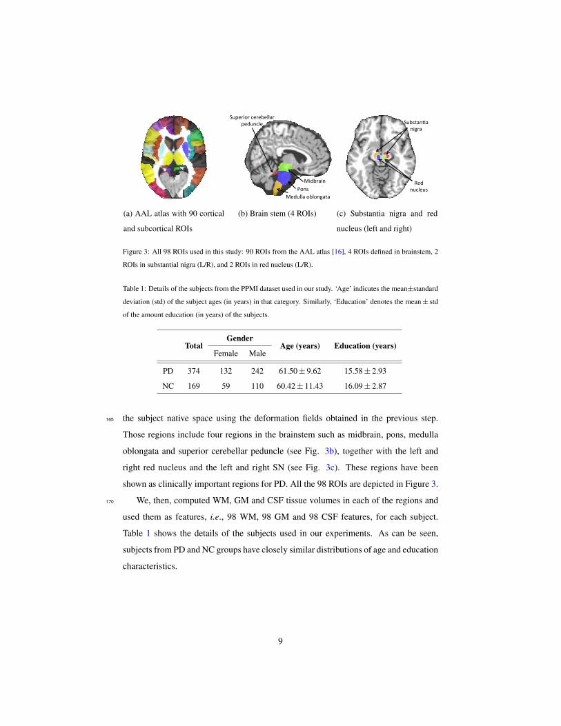
All the MR images were preprocessed by skull stripping [31], cerebellum removal,160

and tissue segmentation into white matter (WM), gray matter (GM), and cerebrospinal

fluid (CSF) [32]. The anatomical automatic labeling (AAL) atlas [16], parcellated with

90 predefined regions, was registered using HAMMER3 [33, 31] to the native space

of each subject. We further added eight regions in the template to be transferred to

2http://www.ppmi-info.org/wp-content/uploads/2013/09/PPMI-WW-ADNI.pdf3Could be downloaded at http://www.nitrc.org/projects/hammerwml

8

AAL#atlas#with#90#cor0cal#and#subcor0cal#ROIs# Brain#stem#(4#ROIs)# Substan0a#nigra#and#red#

nucleus#(L/R)#

Medulla#oblongata#Pone#

Midbrain#

Superior#cerebellar#peduncle# Substan0a#

nigra#

Red#nucleus#

(a) AAL atlas with 90 cortical

and subcortical ROIs

AAL#atlas#with#90#cor0cal#and#subcor0cal#ROIs# Brain#stem#(4#ROIs)# Substan0a#nigra#and#red#

nucleus#(L/R)#

Medulla#oblongata#Pons#

Midbrain#

Superior#cerebellar#peduncle# Substan0a#

nigra#

Red#nucleus#

(b) Brain stem (4 ROIs)AAL#atlas#with#90#cor0cal#and#subcor0cal#ROIs# Brain#stem#(4#ROIs)# Substan0a#nigra#and#red#

nucleus#(L/R)#

Medulla#oblongata#Pone#

Midbrain#

Superior#cerebellar#peduncle# Substan0a#

nigra#

Red#nucleus#

(c) Substantia nigra and red

nucleus (left and right)

Figure 3: All 98 ROIs used in this study: 90 ROIs from the AAL atlas [16], 4 ROIs defined in brainstem, 2

ROIs in substantial nigra (L/R), and 2 ROIs in red nucleus (L/R).

Table 1: Details of the subjects from the PPMI dataset used in our study. ‘Age’ indicates the mean±standard

deviation (std) of the subject ages (in years) in that category. Similarly, ‘Education’ denotes the mean± std

of the amount education (in years) of the subjects.

TotalGender

Age (years) Education (years)Female Male

PD 374 132 242 61.50± 9.62 15.58± 2.93

NC 169 59 110 60.42± 11.43 16.09± 2.87

the subject native space using the deformation fields obtained in the previous step.165

Those regions include four regions in the brainstem such as midbrain, pons, medulla

oblongata and superior cerebellar peduncle (see Fig. 3b), together with the left and

right red nucleus and the left and right SN (see Fig. 3c). These regions have been

shown as clinically important regions for PD. All the 98 ROIs are depicted in Figure 3.

We, then, computed WM, GM and CSF tissue volumes in each of the regions and170

used them as features, i.e., 98 WM, 98 GM and 98 CSF features, for each subject.

Table 1 shows the details of the subjects used in our experiments. As can be seen,

subjects from PD and NC groups have closely similar distributions of age and education

characteristics.

9

3. Overview of the Method175

As discussed earlier, we first process the MR images and obtain tissue segmented

images, after which the anatomical automatic labeling (AAL) atlas is non-linearly reg-

istered to the original MR image space of each subject. From each of the ROIs, we

extract the WM, GM and CSF volumes as features. These features form X, and the

corresponding labels form y. To formulate the problem, we consider N training sam-180

ples, each with d = 98 × 3 = 294 dimensional feature vector. Note that we have

98 ROIs, each of which are represented by 3 tissue-volume features. Let X ∈ RN×d

denote the training data, in which each row indicates a training sample, and y ∈ RN

their corresponding labels. The goal is to determine the labels for the testing samples,

Xtst ∈ RNtst×d.185

Using our proposed joint feature-sample selection (JFSS), some uninformative fea-

tures and samples are discarded, leading to X and y. Note that N samples and d

features are selected, resulting in a new data matrix, X ∈ RN×d, and training labels,

y ∈ RN . It is important to remark that the same Ntst testing samples will now have

d features each, Xtst ∈ RNtst×d. After obtaining the subset of features and samples,190

we train a robust linear discriminant analysis (RLDA) to learn a classification model.

In this process, we jointly decompose X into cleaned data, D, and its noise compo-

nent, E. The classification model is learned on the cleaned data, in order to avoid any

probable noise effects. This procedure is visualized in Figure 2.

Note that, throughout this paper, bold capital letters denote matrices (e.g., X). All195

non-bold letters denote scalar variables. xij denotes the scalar in the row i and col-

umn j of X. 〈x1,x2〉 denotes the inner product between two vectors x1 and x2.

‖x‖22 = 〈x,x〉 =∑i x

2i denotes the squared Euclidean Norm of x. ‖X‖∗ desig-

nates the nuclear norm (sum of singular values) of X. ‖x‖1 =∑i |xi| denotes the `1

norm of the vector x.200

4. The Proposed Joint Feature-Sample Selection (JFSS) Algorithm

The first task is to reliably select the most discriminative features, along with the

best samples to build a classification model. During this process, since the poorly

10

shaped samples are discarded and most discriminative features are selected, it can not

only improve the generalization capability of the learned model, but also speed up the205

learning process. In many real-world applications, it is a cumbersome task to acquire

samples and features for the learning task. Particularly in our application, feature vec-

tors extracted from MRI data are quite prone to noise. Therefore, the data from some

of the subjects might not be useful and might mislead the learning procedure. This mo-

tivates us to select the best samples for learning a diagnosis model. On the other hand,210

as described before, we parcellate brain images into a number of ROIs and represent

each subject by concatenating the features from these ROIs. However, brain neurode-

generative diseases are not reflected on all these ROIs. This further motivates us to

select the most discriminative features. Since, features are extracted from ROIs, select-

ing the most discriminative features also reveals the most crucial brain ROIs related to215

the specific disease (such as PD in our case).

4.1. Formulation

As discussed earlier, these two sub-problems (feature selection and sample selec-

tion) were generally targeted separately. However, feature selection and sample se-

lection affect each other, making separate selections open to more defective feature-220

sample subsets. In other words, separate selections might limit the subsequent classifi-

cation performance in terms of overall learning model accuracy. In this subsection, we

propose a novel feature-sample selection framework in a joint formulation, to guarantee

the selection of best and most discriminative subsets in both domains.

To this end, the selected samples and features should best describe a regression225

model, in terms of the overall accuracy. Without the loss of generality, we employ a

linear regression model. In order to select the most discriminative subset, we consider

sparsity both in feature and sample domains. Recently, the linear sparse regression

model has been widely used for feature selection [24], in which a sparse weight vec-

tor βββ is learned to best predict the training labels. More formally, we would like to230

minimize ‖y−Xβββ‖22, while keeping the coefficient vector, βββ, sparse. But, this feature

selection procedure might be misled if there were noisy features and poor samples. In

this way, we propose to jointly select features and samples through constructing a lin-

11

ear regression model. This would account for the noisy/redundant information in both

domains, simultaneously.235

For this purpose, we introduce two vectors ααα and βββ, used to select samples and

features, respectively. To get the most compact and sparse set in both domains, we

need to impose `0 regularizations on both ααα and βββ. Our joint feature-sample selection

(JFSS) is thus formulated as

minααα,βββ

‖ααα(y −Xβββ

)‖22 + λ1‖βββ‖0 + λ2‖ααα‖0,

subject to ααα = diag(ααα).(1)

The first term controls the overall data fitting error only for the selected samples

indicated by ααα. The second and third terms are to ensure the selection of the smallest

number of the most meaningful samples and features. λ1, λ2 > 0 are the optimiza-

tion hyperparameters, controlling the level of contribution of each term in the entire

optimization process.240

The minimization process of the objective function in (1) is not computationally

tractable. This is because the `0 term is not a convex function and optimizing its

associated variable is as difficult as trying all possible subsets of the measurements.

Therefore, we need to consider approximations of the `0 norms. One of the most com-

mon approximations of the `0 regularization for sparse representation is the `1 norm

[34]. Another feasible approximation is to project the solution onto a simplex [35].

As a result, the above objective function could be rewritten as the following, using `1

approximations for sparsity:

minααα,βββ

‖ααα(y −Xβββ

)‖22 + λ1‖βββ‖1 + λ2‖ααα‖1,

subject to ααα = diag(ααα).(2)

As we would like our method to at least select a minimum number of samples, to

avoid overfitting and prevent from getting trivial solutions, we propose to interpret the

coefficients inααα as probabilities and impose the condition that ∀iαααi ≥ 0 and∑Ni=1αααi =

1. This is equal to projecting the `1-ball onto the simplex as in [35, 36]. Moreover, this

constraint makes the third regularization term in (2) constant, and thus the problem245

12

reduces to:

minααα,βββ

‖ααα(y −Xβββ

)‖22 + λ1‖βββ‖1,

subject to ααα>1 = 1,ααα ≥ 0, ααα = diag(ααα).(3)

Note that the solution to the above objective function for ααα is indeed sparse, be-

cause of the simplex constraints [35, 36]. It is also noteworthy that with this formu-

lation, the algorithm is dependent on less hyperparameters, making it quite appealing

for applications with large and diverse data, in which selecting the hyperparameter is250

burdensome.

4.2. Optimization

The solution to the objective function (3) is not very easy to achieve, as the first term

introduces a quadratic optimization term. In order to solve the optimization problem,

we use an alternating optimization procedure, in which we break the problem down into255

two sub-problems and then solve them iteratively. When fixing each of the associated

variables, the resulting sub-problems would be convex. As studied in the literature, in

such problems, the main objective function can converge to the optimal point [37].

In each iteration, we optimize the objective function by fixing one of the optimiza-

tion variables, while solving for the other, until convergence. Specifically, optimizing

for βββ, while fixing ααα and therefore ααα, would reduce to

minβββ

‖αααy − αααXβββ‖22 + λ1‖βββ‖1. (4)

Similarly, the optimization step for ααα, while fixing βββ, is:

minααα

‖ααα(y −Xβββ

)‖22,

subject to ααα>1 = 1,ααα ≥ 0, ααα = diag(ααα).(5)

The first sub-problem is similar to the standard sparse regression formulation, and

very easy to solve with any standard solver or with the alternating direction method

of multipliers (ADMM) [38]. We introduce an auxiliary variable, b, and form the

13

Lagrangian function as below:

L1(βββ,b, γγγ1) =‖αααy − αααXβββ‖22 + λ1‖b‖1+

〈γγγ>1 ,b− βββ〉+ρ12‖b− βββ + γγγ1‖22,

(6)

where γγγ1 is the Lagrangian multiplier and ρ1 > 0 is a penalty hyperparameter. There-

fore, the optimization steps would be formulated as

βββk+1 =(X>ααα2X+ ρ1I

)−1(X>ααα− αααy + ρ1(b

k − γγγk1)),

bk+1 = Sλ1ρ1

(βββk+1 + γγγk1),

γγγk+11 = γγγk

1 + βββk+1 − bk+1.

(7)

Here, Sκ(a) = (a − κ)+ − (−a − κ)+ is the soft thresholding operator or the

proximal operator for the `1 norm [38], and I is the identity matrix. Note that r+ =260

max(r, 0).

In order to solve the second sub-problem, (5), we rewrite it as the following:

minααα

‖(y −Xβββ

)>ααα‖22,

subject to ααα>1 = 1,ααα ≥ 0.

(8)

The most critical step is the projection of the solution onto the probabilistic simplex,

which is formulated as:

minααα

1

2‖ααα− v‖22, subject to ααα>1 = 1,ααα ≥ 0. (9)

where v is the probabilistic simplex, onto which we want to project theαααweight vector,

as also defined in [35, 36, 39]. This can be solved using the accelerated projected

gradient, as in [35, 39], by writing the Lagrangian function as:

L2(ααα,v, γ2, γγγ3) =1

2‖ααα− v‖22 + 〈γ2,ααα>1− 1〉 − 〈γγγ>3 ,ααα〉. (10)

Solving for ααα while keeping the K.K.T. conditions would give us the optimal pro-

jection onto the probabilistic simplex [35, 36]. Therefore, the objective function in

the sub-problem (8) could be optimized through the projected quasi-Newton algorithm

proposed in [40]. We initialize the vectorααα inversely related to the prediction power of

the samples:

ααα =σ

y −Xβββ + δ, (11)

14

where δ is a small positive number to avoid devision by zeros and σ is a scaling factor.

In the experiments, these two parameters are fixed as δ = 0.0001 and σ = 0.01,

respectively.

Subsequently, the solution to the main problem, as in (3), is obtained by alterna-265

tively solving each of the sub-problems until convergence. The stopping criterion is

that the changes in the two variables ααα and βββ in two consecutive iterations is less than

a threshold (‖αααk −αααk−1‖ < ε and ‖βββk −βββk−1‖ < ε). The penalty hyperparameter ρ1

in (6) controls the convergence rate of the optimization process. It serves as a step size

on how fast to move towards the optimum. If we select a very small value, the solution270

will converge very slowly, whereas, if it has a large value, the step will be very big

and might jump over the optimum. Therefore, a good choice of this hyperparameter

could reduce the convergence time. Many different strategies are used in the literature

to deal with this hyperparameter. Similar to [41, 42], we first set the hyperparameter to

a small value (ρ11 = 10−4) to take small steps at the beginning. In each next iteration,275

we increase its value by ρk+11 = 1.1ρk1 , so that we take a larger step towards the opti-

mum. This is because, at the beginning, the optimization process starts with randomly

initialized variables and, if we take a larger step, we might mislead the direction to the

optimum and increase the convergence time. But, after a number of iterations, larger

steps would lead to faster convergence.280

4.3. JFSS as a Classifier (JFSS-C)

The above procedure of selecting features and samples could also be used directly

for the classification task. As it is obvious, the first term learns a linear regression

model, in which the weights βββ construct the mapping from the features spaces, X, to

the space of the labels, y. This could be used as a classification tool by discretizing the285

y values into classes.

To build the linear classification model (i.e., y = Xβββ + b, where b is the bias), we

add a single column of 1s to the matrix X (i.e., X = [X 1]). This classification scheme

is used as a baseline method in the experiments, referred to as JFSS-C.

15

5. Robust Classification (Robust LDA)290

Even with selection of the most discriminative features and best samples, there

might still be some noises present in the data. These noise elements of data can ad-

versely influence the classifier learning process. This is the case for almost all real-

world applications, where the data is precepted through inaccurate or noise-prone sen-

sors. This issue has been recently explored in the areas of subspace methods [41, 22],295

machine learning [43] and computer vision [23].

In this section, we introduce a robust classification technique based on the least-

squares formulation of linear disciriminant analysis (LS-LDA). Then, we will apply it

to learn a model, classifying our selected samples and features. Note that the feature

and sample selections were performed on the training data. This procedure discarded300

the entire features or samples (columns or rows) in X. But the selected subset might

still have some amounts of noisy elements. Furthermore, it is quite probable that the

testing data were also contaminated with noise. Therefore, a de-noising procedure, for

both training and testing data, could play a very important role on the testing stage and

the overall performance. Note that the de-noising of testing samples is less studied305

in the literature, or is simply performed in an unsupervised manner. We introduce a

procedure to de-noise the testing samples based on the cleaned training data.

5.1. Training

To suppress the possible noise in the data, while learning the classification model,

we need to model the noise in the feature matrix. In other words, we account for the

intra-sample outliers in X to further reduce the influences of noise elements in the

data. For this purpose, following [41, 43], we assume that the data matrix X could be

spanned on a low-rank subspace and, therefore, should be rank-deficient. This assump-

tion supports the fact that samples from the same class are correlated [43, 23]. In order

to achieve a robust classifier, we use a similar idea as in [23], which was proposed for

robust regression. In our case, classification is posed as a binary regression problem, in

which a transform, w, maps each sample in X to a binary label in y. In the linear case,

this could be modeled with a linear discriminant analysis (LDA) through learning a

16

linear mapping to minimize the intra-class discrimination and maximize the inter-class

variation. An extension of LDA, namely LS-LDA [22], models the LDA problem in a

least-squares formulation:

minw‖(y − Xw)y>y‖22, (12)

where w ∈ Rd is a projection of X to the space of labels, y. Note that y>y is a

weighing factor to compensate for an unbalanced number of samples in each of the310

two classes [22].

If the data matrix X is corrupted by noise, we can model the noise by consid-

ering X = D + E, where D ∈ RN×d is the underlying noise-free component and

E ∈ RN×d is the noise component. To model this noise in the above formulation and

learn the mapping w from the clean data D, we utilize the scenario in [23]. Analo-

gous to the robust principal component analysis (RPCA) formulation [44], it could be

assumed that the noise-free component of the data is spanned on a low-rank subspace.

Correspondingly, the error matrix is assumed to be a sparse matrix, as we are not ex-

pecting a huge amount of elements to be contaminated by noise. This is because the

JFSS procedure selects the most relevant features and the best samples. Therefore, lots

of original data contaminated with noise are already removed. The remaining data are

those with the most correlation to the labels. But, there is still a possibility that some

random noise is remaining in the selected features. Considering these, we can rewrite

our problem as:

minw,D,D,E

η

2‖(y − Dw)y>y‖22 + ‖D‖∗ + γ‖E‖1,

subject to X = D+E, D = [D 1],

(13)

where the first term learns the mapping w from the clean data and projects the samples

to the label space. The second and the third terms guarantee the rank-deficiency of

the data matrix D and the sparsity of the matrix E, respectively. These two terms are

similar to RPCA [44].315

Note that RPCA is an unsupervised method, which de-noises the data matrix with-

out considering the data labels. Whereas, the above formulation cleans the data in a

supervised manner. Particularly, matrix D retains the subspace of X, which is most

17

correlated to the labels y.

The solution to problem (13) could be achieved by writing the Lagrangian function,320

and iteratively solving for w, D, D and E one at a time, while fixing others [23], using

the augmented Lagrangian method (ALM) of multipliers technique.

5.2. Testing

In the testing phase, the probable noise present in the samples can dramatically

affect the classification accuracy. De-noising the testing samples is a challenging task,325

as we do not have any label and class information for them; thus we cannot perform

the supervised de-noising procedure, as we did for the training samples.

To clean the testing data, one can use RPCA [44, 45], but as discussed before, it is

an unsupervised approach. To this end, we utilize the samples cleaned in the training

stage, D, in a supervised manner. The de-noising procedure for the testing data, Xtst,

would consist of representing the testing sample as a linear combination of the training

data samples:

Dtst = DZtst, (14)

where Ztst is the coefficient matrix for the combination. But, to account for the noise

in the testing samples, we add a noise element and reformulate the combination as:

Xtst = DZtst +Etst, (15)

where Etst ∈ RNtst×d is the noise component of the testing data. To acquire the best

linear combination, for representing the testing samples, it is important to ensure that

each sample is represented only by a small number of the training samples. Because

samples come from different classes and the samples could best be de-noised if they

are represented by the most similar samples to them. As a result, in order for the linear

combination to be locally compact, we further impose the low-rank constraint on the

coefficients, as in [41, 46]:

minZtst,Etst

‖Ztst‖∗ + λ‖Etst‖1,

subject to Xtst = DZtst +Etst.

(16)

18

This optimization problem could be solved using linearized ALM method as in

[46]. After cleaning the testing data, the prediction for the classification output is

calculated as

ytst = [DZtst 1]w. (17)

Same as in LS-LDA [22], ytst is used as the decision value, and the binary class

labels are produced using the k-nearest neighbor strategy.

6. Experiments330

As discussed earlier, the proposed JFSS discards poor samples and irrelevant fea-

tures to build a linear regression model that can predict subject categories. In order to

validate the proposed JFSS procedure, we first construct a set of synthetic data to eval-

uate the behavior of the method against noisy samples and redundant features. Then,

the proposed procedure is used to diagnose PD patients. As described earlier, subjects335

from the PPMI database are used for this study.

All results are generated using a 10-fold cross validation strategy. The best hyper-

parameters for our method are selected using a grid search with all possible values for

each hyperparameter. To be fair, the results for the baseline methods were also gen-

erated using a similar 10-fold cross validation strategy and, similar to our method, the340

best hyperparameters for each of the methods were selected. Specifically, the hyperpa-

rameters were set using an inner 10-fold cross validation, where the training data itself

was split into 10 partitions and then a 10-fold cross validation procedure determined

the best set of the hyperparameters for the method. The best values for each of the

hyperparameters in Equations (3), (13) and (16) are separately optimized in the range345

[10−5, 1].

In order to evaluate the proposed approach, different baseline methods are incor-

porated. Baseline classifiers under comparison include linear support vector machines

(SVM), sparse SVM [47], matrix completion (MC) [43], sparse regression (SR), JFSS

as a classifier (JFSS-C) as described in Section 4, and the original least-squares linear350

discriminant analysis (LS-LDA) [22]. Matrix completion is a transductive classifica-

tion approach that deals with the noise in feature values and can suppress a controlled

19

amount of sparse noise in both training and testing feature vectors [43]. It has shown a

good performance in many applications recently [48, 49]. MC, like our method, incor-

porates a sparse noise model to de-noise the data. On the other hand, it de-noises both355

training and testing data. Therefore, in order to provide extensive comparative studies,

we compare the results from MC against the results obtained by our approach.

As for feature and sample selection, to evaluate the proposed JFSS procedure, we

compare the results with separate feature and sample selections (FSS), sparse feature

selection (SFS), and no feature sample selection (no FSS). These three methods pro-360

vide direct baseline methods for the proposed JFSS, since they use a similar approach

for selecting samples and features. Note that for the SR classification scheme, as de-

scribed above, we only report results for FSS and SFS. Furthermore, we report re-

sults using other prominent methods for feature transform or reduction like the popular

min-redundancy max-relevance (mRMR) [26], principal component analysis (PCA),365

robust principal component analysis (RPCA) [44], autoencoder-restricted Boltzmann

machine (AE-RBM) [25], and non-negative matrix factorization (NNMF) [50]. These

five methods are of the state-of-the-art methods widely used for feature reduction or

transformation, compared to which we can demonstrate the significant improvements

by the proposed method.370

An important characteristics of the proposed JFSS method was to select the best

set of samples (along with features) to build a classification model. One of the most

popular approaches for removing outliers is RANSAC [51]. RANSAC is a consen-

sus resampling technique, which randomly subsamples the input data and constructs

models, iteratively. In each iteration, if the selected samples result in a smaller inlier

error, the classification model parameters are updated. The procedure starts by ran-

domly selecting the minimum number of samples (denoted by m) required to build the

classification model, after which the classifier is trained, using the randomly selected

samples. Then, the whole set of samples from the training set is examined with the

built model and the number of inliers is determined. If the fraction of the number of

inliers over the total number of samples exceeds a certain threshold τ , the classifier is

again built using all the identified inliers and the procedure is terminated. Otherwise,

this procedure is iterated at least N times to ensure the selection of an appropriate set of

20

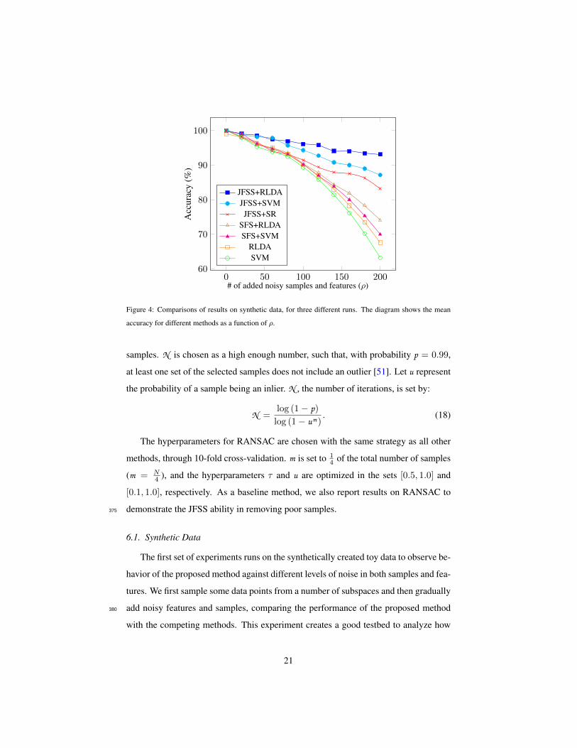
0 50 100 150 20060

70

80

90

100

# of added noisy samples and features (ρ)

Acc

urac

y(%

)JFSS+RLDAJFSS+SVMJFSS+SR

SFS+RLDASFS+SVM

RLDASVM

Figure 4: Comparisons of results on synthetic data, for three different runs. The diagram shows the mean

accuracy for different methods as a function of ρ.

samples. N is chosen as a high enough number, such that, with probability p = 0.99,

at least one set of the selected samples does not include an outlier [51]. Let u represent

the probability of a sample being an inlier. N , the number of iterations, is set by:

N =log (1− p)log (1− um)

. (18)

The hyperparameters for RANSAC are chosen with the same strategy as all other

methods, through 10-fold cross-validation. m is set to 14 of the total number of samples

(m = N4 ), and the hyperparameters τ and u are optimized in the sets [0.5, 1.0] and

[0.1, 1.0], respectively. As a baseline method, we also report results on RANSAC to

demonstrate the JFSS ability in removing poor samples.375

6.1. Synthetic Data

The first set of experiments runs on the synthetically created toy data to observe be-

havior of the proposed method against different levels of noise in both samples and fea-

tures. We first sample some data points from a number of subspaces and then gradually

add noisy features and samples, comparing the performance of the proposed method380

with the competing methods. This experiment creates a good testbed to analyze how

21

our method can select the best samples and features and suppress noise, compared to

different baseline methods.

To this end, we construct two independent subspaces of dimensionality 100, same

as described in [41], and sample 500 samples from each subspace, which could create a385

binary classification problem. The two subspaces S1, S2 are constructed with bases U1

and U2. U1 ∈ R100×100 is a random orthogonal matrix and U2 = TU1, in which T is

a random rotation matrix. Then, 500 vectors are sampled from each subspace through

Xi = UiQi, i = {1, 2} with Qi, a 100 × 500 matrix, independent and identically

distributed (i.i.d.) from N (0, 1).390

In order to evaluate the robustness of the method in both sample and feature spaces,

we gradually add a certain number of additional noisy samples and features to the data.

Specifically, we add ρ randomly generated features and ρ randomly generated samples

to the data, and then run the proposed and the baseline methods. All noisy data are

drawn i.i.d. from N (0, 1). Since our method jointly performs both sample and feature395

selections, we increase the noise level in both domains. Figure 4 shows the mean

accuracy results of three different runs, as a function of the additional number of noisy

features and samples, with a 10-fold cross-validation strategy. The mean and standard

deviation values could be found in Table 2, as well. The reported results for all the

methods are achieved with their best tuned hyperparameters. To analyze the effects400

of the only hyperparameter (λ1) associated with JFSS, we plot the accuracy of two

classification techniques (SVM and RLDA) as a function of the parameter in Figure

5. The diagram is plotted for the case that the number of added noisy features and

sample, ρ, is equal to 100. As can be seen, the classification performance is partially

independent from the hyperparameter and, in a sensible range of the values for the405

hyperparameter, we consistently achieve reasonable results.

Our JFSS coupled with any of the classifiers has the ability to select better subset

of features and samples and achieve satisfactory results. However, when the RLDA

classification scheme is used, it acts more robust against the increase of noise elements

(as can be seen in Figure 4). This is attributed to the de-noising process introduced by410

our RLDA. As discussed earlier, with RLDA, we de-noise the testing samples as well,

while for other classifiers the testing samples are intact. Note that, these testing samples

22

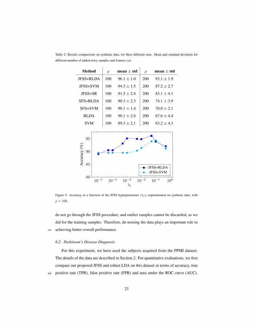
Table 2: Results comparisons on synthetic data, for three different runs. Mean and standard deviation for

different number of added noisy samples and features (ρ).

Method ρ mean ± std ρ mean ± std

JFSS+RLDA 100 96.1 ± 1.0 200 93.1 ± 1.9

JFSS+SVM 100 94.3 ± 1.5 200 87.2 ± 2.7

JFSS+SR 100 91.5 ± 2.4 200 83.1 ± 4.1

SFS+RLDA 100 90.3 ± 2.3 200 74.1 ± 3.9

SFS+SVM 100 90.1 ± 1.4 200 70.0 ± 2.1

RLDA 100 90.1 ± 2.6 200 67.6 ± 4.4

SVM 100 89.3 ± 2.1 200 63.2 ± 4.3

10−5 10−4 10−3 10−2 10−1 10080

85

90

95

λ1

Acc

urac

y(%

)

JFSS+RLDAJFSS+SVM

Figure 5: Accuracy as a function of the JFSS hyperparameter (λ1), experimented on synthetic data, with

ρ = 100.

do not go through the JFSS procedure, and outlier samples cannot be discarded, as we

did for the training samples. Therefore, de-noising the data plays an important role in

achieving better overall performance.415

6.2. Parkinson’s Disease Diagnosis

For this experiment, we have used the subjects acquired from the PPMI dataset.

The details of the data are described in Section 2. For quantitative evaluations, we first

compare our proposed JFSS and robust LDA on this dataset in terms of accuracy, true

positive rate (TPR), false positive rate (FPR) and area under the ROC curve (AUC).420

23

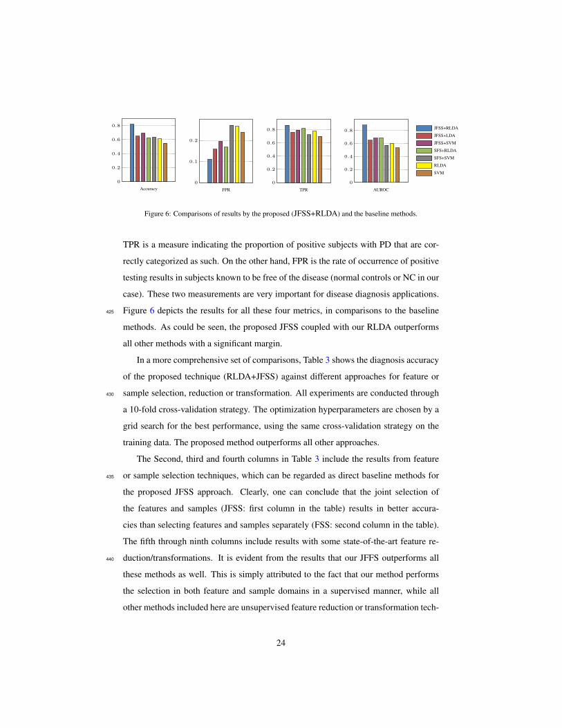
Accuracy

0

0.2

0.4

0.6

0.8

FPR

0

0.1

0.2

TPR

0

0.2

0.4

0.6

0.8

AUROC

0

0.2

0.4

0.6

0.8JFSS+RLDA

JFSS+LDA

JFSS+SVM

SFS+RLDA

SFS+SVM

RLDA

SVM

Figure 6: Comparisons of results by the proposed (JFSS+RLDA) and the baseline methods.

TPR is a measure indicating the proportion of positive subjects with PD that are cor-

rectly categorized as such. On the other hand, FPR is the rate of occurrence of positive

testing results in subjects known to be free of the disease (normal controls or NC in our

case). These two measurements are very important for disease diagnosis applications.

Figure 6 depicts the results for all these four metrics, in comparisons to the baseline425

methods. As could be seen, the proposed JFSS coupled with our RLDA outperforms

all other methods with a significant margin.

In a more comprehensive set of comparisons, Table 3 shows the diagnosis accuracy

of the proposed technique (RLDA+JFSS) against different approaches for feature or

sample selection, reduction or transformation. All experiments are conducted through430

a 10-fold cross-validation strategy. The optimization hyperparameters are chosen by a

grid search for the best performance, using the same cross-validation strategy on the

training data. The proposed method outperforms all other approaches.

The Second, third and fourth columns in Table 3 include the results from feature

or sample selection techniques, which can be regarded as direct baseline methods for435

the proposed JFSS approach. Clearly, one can conclude that the joint selection of

the features and samples (JFSS: first column in the table) results in better accura-

cies than selecting features and samples separately (FSS: second column in the table).

The fifth through ninth columns include results with some state-of-the-art feature re-

duction/transformations. It is evident from the results that our JFFS outperforms all440

these methods as well. This is simply attributed to the fact that our method performs

the selection in both feature and sample domains in a supervised manner, while all

other methods included here are unsupervised feature reduction or transformation tech-

24

Table 3: Accuracy of the PD/NC classification, compared among baseline classifiers and different feature-

sample selection or reduction techniques. First column shows the results for the proposed joint feature-

sample selection method. The second, third and fourth columns include the results with separate feature and

sample selection, sparse feature selection, and no feature or sample selections, respectively. The next five

columns show the results for some state-of-the-art feature reduction techniques, and finally the last column

shows the results for the well-known RANSAC algorithm for outlier sample removal. Note that ∗ stands for

the case with p < 0.05 and † for p < 0.01 in a cross-validated 5 × 2 t-test against the proposed method

(RLDA+JFSS).

ClassifierSelection/Reduction Method

JFSS FSS SFS no FSS mRMR PCA RPCA AE-RBM NNMF RANSAC

Robust LDA 81.9 78.0∗ 67.7† 61.5† 70.5† 65.0† N/A 76.8∗ 64.5† 74.7†

MC 78.9∗ 73.5† 66.0† 56.2† 69.2† 62.4† N/A 73.1† 64.1† 72.3†

LDA 65.9† 62.1† 61.5† 56.0† 60.9† 56.0† 60.5† 65.1† 58.1† 66.0†

SVM 69.1† 61.9† 61.1† 55.5† 58.8† 58.5† 61.0† 66.6† 59.1† 71.2†

Sparse SVM 70.1† 62.8† 6.15† 59.5† 60.0† 59.3† 61.8† 68.7† 63.1† 73.1†

SR N/A 61.6† 59.6† N/A 60.5† 59.9† 60.6† 63.7† 61.5† 64.2†

JFSS-C 68.7† N/A N/A N/A 67.5† 68.8† 71.9† 72.8† 67.0† 69.9†

niques. Furthermore, for our application, the features come from the brain ROIs. Since

not all the brain regions are associated with PD, many of the features are redundant.445

This is why these feature reduction techniques perform worse than our feature selection

scheme. In the context of feature selection, we only select the most relevant features,

while the feature reduction techniques transform the whole set of features (all with

equal contributions) to a lower dimension space. The last column in the table shows

the results from the RANSAC technique for outlier sample removal [51]. Again, the450

proposed JFSS shows to select a much better set of samples along with their respective

features for the task of PD diagnosis.

It is worth noting that the SR classification technique, which is used as a baseline

method, is directly derived from the weights learned in FSS and SFS. Therefore, when

using SFS and FSS, we can report results for SR. We further ran the sparse regression455

on the outputs of other feature reduction techniques and reported results in Table 3. In

25

addition, the last row of the table contains results form JFSS as a classifier (JFSS-C),

explained in Section 4. JFSS-C is, in fact, the original JFSS, which can be directly used

to build the classification model. So, JFSS and JFSS-C are not two separate procedures,

and that’s why we do not couple JFSS-C with other feature selection methods. As can460

be seen, JFSS-C can produce comparable results with LDA or SVM coupled with our

JFSS, while it is much better than LDA, SVM or even RLDA when no feature or sample

selection is conducted.

One of the most important baselines to the de-nosing aspect of the proposed method

could be the RPCA approach, which de-noises the data through the same low-rank465

assumption on the data matrix. Therefore, we apply RPCA on the training data to de-

noise the samples and their feature vectors and then apply a variety of classifiers to

classify them. The results could be seen in the seventh row of Table 3. The RLDA

and MC classifiers implicitly de-noise the data through a same low-rank minimization

procedure, and therefore we did not couple RPCA with them.470

Additionally, a statistical analysis is performed on the results and reported in Table

3. In order to statistically analyze the significance of the achieved results, a cross-

validated 5 × 2 t-test [52] is performed on the accuracy results of each competing

method against our proposed method (JFSS+RLDA). As discussed in detail in [53,

54, 52], this statistical test yields more reliable results for statistically analyzing the475

classifier performances, compared to the conventional paired t-tests. In particular, we

perform 5 different replications of a 2-fold cross-validation. In each of the replica-

tions, the data is randomly split into two sets. The results from the first set of the five

replications are used to estimate the mean difference, and the results of all folds are

incorporated to estimate the variance. Then, a t-statistic is calculated to achieve the p-480

value, showing the significance of the comparison on the results. The details of the test

are explained in [52]. In Table 3, the methods with a p-value of p < 0.05 are indicated

with a ∗ symbol and the results with p < 0.01 are indicated with a † symbol. As can

be seen, our proposed method achieves statistically significant results compared to all

other methods. Furthermore, we also perform a permutation test [54] on the proposed485

method, which is a non-parametric method without assuming any data distribution, to

assess whether the proposed classifier has found a class structure (a connection be-

26

10−5 10−4 10−3 10−2 10−1 10050

60

70

80

λ1

Acc

urac

y(%

)

JFSS+RLDAJFSS+MCJFSS+LDAJFSS+SVM

JFSS-C

Figure 7: Accuracy as a function of the JFSS hyperparameter (λ1), for the Parkinson’s disease diagnosis

experiment.

tween the data and their respective class labels), or the observed accuracy was obtained

by chance. In order to perform this test, we repeat the classification procedure by ran-

domly permuting the class labels for τ different times (τ = 100, in our experiments).490

The p-value can then be calculated as the percentage of runs for which the obtained

classification error is better than the original classification error. After performing the

test, we get a p-value smaller than 0.05, which indicates that the classification error

on the original data is indeed significantly small and, therefore, the classifier is not

randomly generating those results [54].495

In addition, to analyze the effect of the hyperparameter on the accuracy of the

methods, the proposed JFSS method was put together with all classifiers and the best

achieved accuracy for each set of hyperparameters and classifiers is plotted in Figure

7. As can be seen, the first two methods, which perform de-noising while learning the

classifier model, behave similarly, while JFSS+RLDA leads to a better performance. In500

general, changing the hyperparameter influences the selected features, and that is why

the classifiers perform differently under different hyperparameter settings. In order to

further investigate the effect of the hyperparameters, we plot the performance of the

competing classifiers, with the JFSS parameters fixed, as a function of their respective

hyperparameter. Figure 8 shows these results for three major methods in comparison.505

Specifically, the diagram on the left analyzes the hyperparameter λ of matrix com-

27

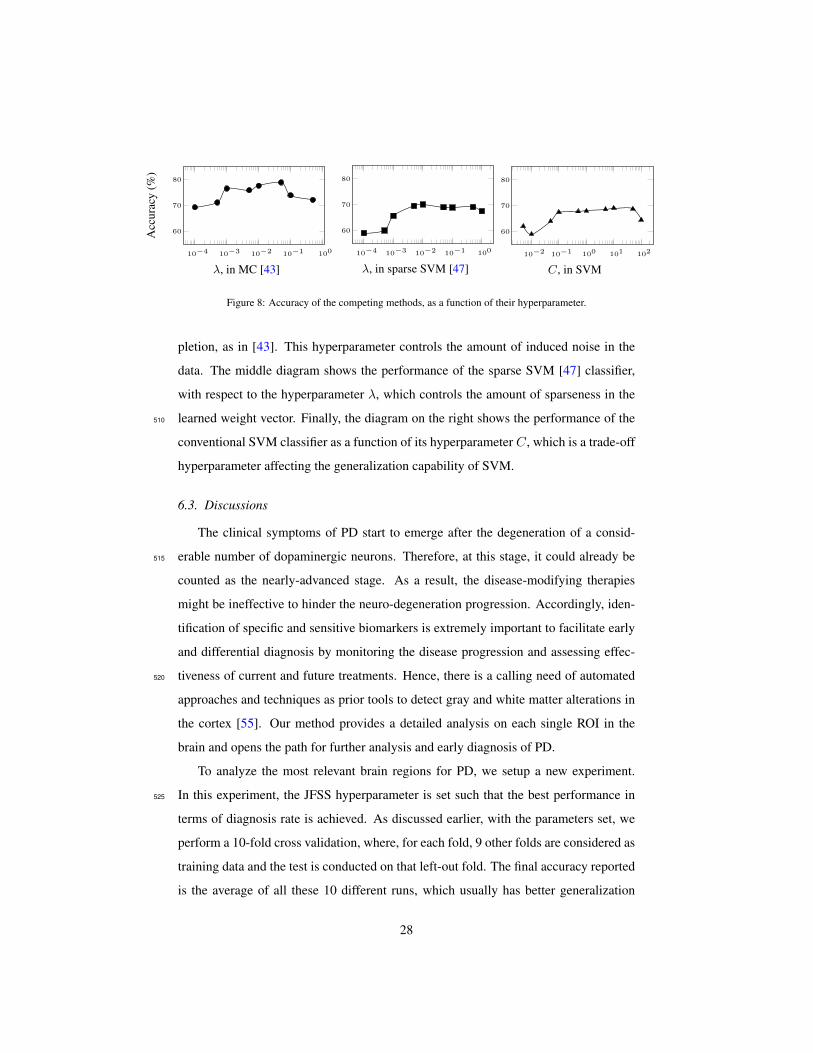
10−4 10−3 10−2 10−1 100

60

70

80

λ, in MC [43]

Acc

urac

y(%

)

10−4 10−3 10−2 10−1 100

60

70

80

λ, in sparse SVM [47]10−2 10−1 100 101 102

60

70

80

C, in SVM

Figure 8: Accuracy of the competing methods, as a function of their hyperparameter.

pletion, as in [43]. This hyperparameter controls the amount of induced noise in the

data. The middle diagram shows the performance of the sparse SVM [47] classifier,

with respect to the hyperparameter λ, which controls the amount of sparseness in the

learned weight vector. Finally, the diagram on the right shows the performance of the510

conventional SVM classifier as a function of its hyperparameter C, which is a trade-off

hyperparameter affecting the generalization capability of SVM.

6.3. Discussions

The clinical symptoms of PD start to emerge after the degeneration of a consid-

erable number of dopaminergic neurons. Therefore, at this stage, it could already be515

counted as the nearly-advanced stage. As a result, the disease-modifying therapies

might be ineffective to hinder the neuro-degeneration progression. Accordingly, iden-

tification of specific and sensitive biomarkers is extremely important to facilitate early

and differential diagnosis by monitoring the disease progression and assessing effec-

tiveness of current and future treatments. Hence, there is a calling need of automated520

approaches and techniques as prior tools to detect gray and white matter alterations in

the cortex [55]. Our method provides a detailed analysis on each single ROI in the

brain and opens the path for further analysis and early diagnosis of PD.

To analyze the most relevant brain regions for PD, we setup a new experiment.

In this experiment, the JFSS hyperparameter is set such that the best performance in525

terms of diagnosis rate is achieved. As discussed earlier, with the parameters set, we

perform a 10-fold cross validation, where, for each fold, 9 other folds are considered as

training data and the test is conducted on that left-out fold. The final accuracy reported

is the average of all these 10 different runs, which usually has better generalization

28

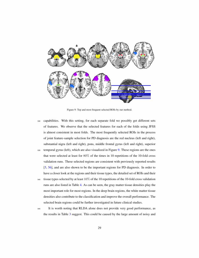
Figure 9: Top and most frequent selected ROIs by our method.

capabilities. With this setting, for each separate fold we possibly get different sets530

of features. We observe that the selected features for each of the folds using JFSS

is almost consistent in most folds. The most frequently selected ROIs in the process

of joint feature-sample selection for PD diagnosis are the red nucleus (left and right),

substantial nigra (left and right), pons, middle frontal gyrus (left and right), superior

temporal gyrus (left), which are also visualized in Figure 9. These regions are the ones535

that were selected at least for 80% of the times in 10 repetitions of the 10-fold cross

validation runs. These selected regions are consistent with previously reported results

[5, 56], and are also shown to be the important regions for PD diagnosis. In order to

have a closer look at the regions and their tissue types, the detailed set of ROIs and their

tissue types selected by at least 10% of the 10 repetitions of the 10-fold cross validation540

runs are also listed in Table 4. As can be seen, the gray matter tissue densities play the

most important role for most regions. In the deep brain regions, the white matter tissue

densities also contribute to the classification and improve the overall performance. The

selected brain regions could be further investigated in future clinical studies.

It is worth noting that RLDA alone does not provide very good performance, as545

the results in Table 3 suggest. This could be caused by the large amount of noisy and

29

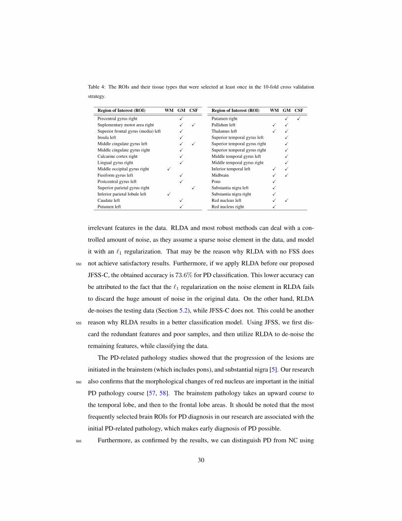
Table 4: The ROIs and their tissue types that were selected at least once in the 10-fold cross validation

strategy.

Region of Interest (ROI) WM GM CSF

Precentral gyrus right XSuplementary motor area right X XSuperior frontal gyrus (media) left XInsula left XMiddle cingulate gyrus left X XMiddle cingulate gyrus right XCalcarine cortex right XLingual gyrus right XMiddle occipital gyrus right XFusiform gyrus left XPostcentral gyrus left XSuperior parietal gyrus right XInferior parietal lobule left XCaudate left XPutamen left X

Region of Interest (ROI) WM GM CSF

Putamen right X XPallidum left X XThalamus left X XSuperior temporal gyrus left XSuperior temporal gyrus right XSuperior temporal gyrus right XMiddle temporal gyrus left XMiddle temporal gyrus right XInferior temporal left X XMidbrain X XPons XSubstantia nigra left XSubstantia nigra right XRed nucleus left X XRed nucleus right X

irrelevant features in the data. RLDA and most robust methods can deal with a con-

trolled amount of noise, as they assume a sparse noise element in the data, and model

it with an `1 regularization. That may be the reason why RLDA with no FSS does

not achieve satisfactory results. Furthermore, if we apply RLDA before our proposed550

JFSS-C, the obtained accuracy is 73.6% for PD classification. This lower accuracy can

be attributed to the fact that the `1 regularization on the noise element in RLDA fails

to discard the huge amount of noise in the original data. On the other hand, RLDA

de-noises the testing data (Section 5.2), while JFSS-C does not. This could be another

reason why RLDA results in a better classification model. Using JFSS, we first dis-555

card the redundant features and poor samples, and then utilize RLDA to de-noise the

remaining features, while classifying the data.

The PD-related pathology studies showed that the progression of the lesions are

initiated in the brainstem (which includes pons), and substantial nigra [5]. Our research

also confirms that the morphological changes of red nucleus are important in the initial560

PD pathology course [57, 58]. The brainstem pathology takes an upward course to

the temporal lobe, and then to the frontal lobe areas. It should be noted that the most

frequently selected brain ROIs for PD diagnosis in our research are associated with the

initial PD-related pathology, which makes early diagnosis of PD possible.

Furthermore, as confirmed by the results, we can distinguish PD from NC using565

30

only MRI. With the progression of PD, patients’ brains are affected heavily with time.

So, these data-driven methods could be of great use for early diagnosis, or prediction of

the disease progression. MRI techniques could be used to monitor disease progression

and to detect brain changes in preclinical patients or in patients at risk of developing

PD. However, to date, these techniques suffer from the lack of standardization, partic-570

ularly the methods for extracting quantitative information from images, and the lack

of validation in large cohorts of subjects in longitudinal studies. Our research partly

resolved the bottleneck restriction.

Our proposed method for classifying the neuroimaging data could be easily em-

ployed for analysis and identification of other brain diseases. To demonstrate that, we575

setup another experiment using the widely researched Alzheimer’s disease neuroimag-

ing initiative (ADNI) database4. The aim is to identify the subjects status, diagnosing

AD and its prodormal stage, known as mild cognitive impairment (MCI). For this pur-

pose, we used 396 subjects (93 AD patients, 202 MCI patients and 101 NC subjects)

from the database, which had complete MRI and FDG-PET data. To process the data,580

tools in [59] and [60] are used for spatial distortion, skull-stripping, and cerebellum

removing. Then, the FSL package [61] was used to segment each MR image into three

different tissues, i.e., gray matter (GM), white matter (WM), and cerebrospinal fluid

(CSF). The subjects are further processed with 93 ROIs [62] parcellated for each [33]

with atlas warping. The volume of GM tissue in each ROI was calculated as the image585

feature. For FDG-PET images, a rigid transformation was employed to align it to the

corresponding MR image and the mean intensity of each ROI was calculated as the

feature. All these features were further normalized in a similar way as in [63]. As a

results, each subject has 2×93 = 186 features. Table 5 lists the results achieved by our

proposed method (JFSS+RLDA) on this data, compared with some baseline methods.590

Two different sets of experiments are conducted to first discriminate NC from MCI

subjects and then NC from AD subjects. Therefore, NC subjects form our negative

class, while the positive class is defined as AD in one experiment and MCI in another

experiment. Table 5 shows the results for the two separate experiments, AD vs. NC and

4http://www.loni.ucla.edu/ADNI

31

Table 5: The accuracy (ACC) and the area under ROC curve (AUC) results of AD diagnosis on the ADNI

database, with comparison to some baseline methods.

JFSS+RLDA JFSS+LDA JFSS+SVM RPCA+LDA RPCA+SVM RLDA LDA SVM

AD/NCACC 91.5 89.4 89.0 89.5 86.1 87.8 82.7 85.4

AUC 0.94 0.90 0.90 0.92 0.88 0.90 0.84 0.85

MCI/NCACC 81.9 79.1 77.3 78.1 80.1 80.3 66.1 74.1

AUC 0.83 0.80 0.75 0.72 0.78 0.82 0.69 0.74

Table 6: Top selected ROIs for the ADNI experiments.

MRI FDG-PET

AD/NC

hippocampal formation right, hippocampal formation left,

middle temporal gyrus left, middle frontal gyrus right, mid-

dle temporal gyrus left, perirhinal cortex left, superior pari-

etal lobule left, lateral occipitotemporal gyrus right, inferior

frontal gyrus left

precuneus right, precuneus left, globus palladus left, tempo-

ral pole right, frontal lobe WM left, middle temporal gyrus

left, postcentral gyrus left, temporal lobe WM left, postcen-

tral gyrus right, medial frontal gyrus right, amygdala left,

amygdala right, thalamus right, occipital pole left

MCI/NC

middle frontal gyrus right, lateral front-orbital gyrus right,

precuneus right, precuneus left, medial front-orbital gyrus

right, inferior frontal gyrus left, inferior occipital gyrus left,

inferior frontal gyrus right, precentral gyrus left, temporal

pole left

globus palladus right, frontal lobe WM right, subthalamic

nucleus left, inferior occipital gyrus left, superior occipital

gyrus right, supramarginal gyrus left, caudate nucleus right,

lingual gyrus left, postcentral gyrus left, parietal lobe WM

right, postcentral gyrus right, Angular gyrus left

MCI vs. NC classifications.595

Similar to the experiment conducted on PD, the top selected regions with the best

parameters are listed in Table 6. The top selected regions are defined as those selected

by at least 50% of the times in 10 repetitions of the 10-fold cross validation runs.

Note that these selected regions are consistently reported as important in the previous

AD/MCI studies [64, 13], as well.600

7. Conclusions

In this paper, we have introduced a joint feature-sample selection (JFSS) frame-

work, along with a robust classification approach for PD diagnosis. We have estab-

32

lished robustness in both training and testing phases. We verified our method using sub-

jects excerpted from the PPMI dataset, a first large-scale longitudinal study of PD. Our605

method outperforms several baseline methods on both synthetic data and the PD/NC

classification problem, in terms of the accuracy of the classification task. Furthermore,

we investigated the biomarkers for PD and have also confirmed the results reported in

the recent and ongoing researches. As a direction for future work, one can use clinical

scores and other imaging modalities to predict PD progression, or to improve predic-610

tion accuracy. More effective features can also be extracted to further enhance the

diagnosis accuracy.

Appendix A. Augmented Lagrangian Method (ALM)

Augmented Lagrangian methods are sets of algorithms for solving problems of

constrained optimization [38]. In these methods, usually the constrained optimization

objective is replaced with one or a series of unconstrained objectives, by adding penalty

terms. These terms are added to mimic a Lagrange multiplier. The general form of an

equality-constrained convex optimization problem would be

minx

f(x)

subject to Ax = b,

(A.1)

where x ∈ Rn, A ∈ Rm×n, b ∈ Rm and f : Rn → R is a convex function. The

Lagrangian function for the above objective would form as follows, by incorporating a

Lagrangian multiplier or a so-called dual variable, y ∈ Rm:

L(x,y) = f(x) + y>(Ax− b). (A.2)

This problem could be solved using the dual ascent method [38, 65], by writing the

dual function and solving for that. But to ensure the convergence, f should be strictly

convex and finite. To solve the problem under more relaxed conditions, the augmented

Lagrangian method of multipliers could be incorporated, by adding a penalty term to

the Lagrangian:

Lρ(x,y) = f(x) + y>(Ax− b) +ρ

2‖Ax− b‖22, (A.3)

33

where ρ > 0 is a penalty hyperparameter that controls the rate of convergence towards

the satisfaction of the constraint, used as a step size. Note that when ρ = 0, L0 is615

the standard Lagrangian function. The advantages of considering the penalty term is

that the dual function would be differentiable under rather mild conditions for problem

(A.1). Therefore, applying dual ascent to the new problem with the penalty term leads

to the following optimization steps on each variable, at each kth iteration:

xk+1 ← argminxLρ(x,yk), (A.4)

yk+1 ← yk + ρ(Axk+1 − b), (A.5)

Appendix A.1. Alternating Direction Method of Multipliers (ADMM)620

When there are more than one optimization variables associated with the problem,

we can take advantage of the decomposability of the dual ascent [38] method and the

convergence superiority of the ALM to solve the problem in a similar way. Suppose

we have a problem modeled as:

minx,z

f(x) + g(z)

subject to Ax+Bz = c,

(A.6)

where x ∈ Rn, z ∈ Rm, A ∈ Rp×n, B ∈ Rp×m and c ∈ Rp. The two functions

f : Rn → R and g : Rm → R are assumed to be the convex functions. As can be

seen in Equation (A.6), there are two variables to be optimized in this new formulation.

Similarly, we can write the augmented Lagrangian as:

Lρ(x, z,y) = f(x) + g(z) + y>(Ax+Bz− c) +ρ

2‖Ax+Bz− c‖22. (A.7)

Here, to optimize the above function, we need to iteratively update each variable

while keeping others fixed. Therefore, the x-minimization, z-minimization, and La-

granigiuan multiplier update steps at the kth iteration have the following forms:

xk+1 ← argminxLρ(x, zk,yk), (A.8)

zk+1 ← argminzLρ(xk+1, z,yk), (A.9)

yk+1 ← yk + ρ(Axk+1 +Bzk+1 − c). (A.10)

34

In this method, the augmented Lagrangian function is minimized jointly with re-

spect to the two associated variables. Each of the variables is updated in a sequential625

order or a so-called alternating fashion. If we have more variables, same strategy can

be incorporated, as long as the problem can be decomposed into sub-problems and the

sub-problems (like in (A.8) and (A.9)) are convex. The stopping criterion in this situa-

tion would the convergence of the main objective, while the constraint(s) are satisfied.

For a more detailed discussion on the methods and their convergence properties, please630

refer to [38, 65].

References

[1] D. B. Miller, J. P. OCallaghan, Biomarkers of parkinsons disease: Present and

future, Metabolism 64 (3, Supplement 1) (2015) S40 – S46.

[2] J. A. Obeso, M. C. Rodriguez-Oroz, M. Rodriguez, J. L. Lanciego, J. Artieda,635

N. Gonzalo, C. W. Olanow, Pathophysiology of the basal ganglia in parkinson’s

disease, Trends in Neurosciences 23, Supplement 1 (2000) S8 – S19.

[3] D. A. Ziegler, J. C. Augustinack, Harnessing advances in structural MRI to en-

hance research on Parkinson’s disease, Imaging in medicine 5 (2) (2013) 91–94.

[4] K. R. Chaudhuri, D. G. Healy, A. H. Schapira, Non-motor symptoms of parkin-640

son’s disease: diagnosis and management, The Lancet Neurology 5 (3) (2006)

235 – 245.

[5] H. Braak, K. Tredici, U. Rub, R. de Vos, E. J. Steur, E. Braak, Staging of brain

pathology related to sporadic parkinsons disease, Neurobio. of Aging 24 (2)

(2003) 197 – 211.645

[6] S. Duchesne, Y. Rolland, M. Varin, Automated computer differential classifica-

tion in parkinsonian syndromes via pattern analysis on MRI, A. Radiology 16 (1)

(2009) 61 – 70.

35

[7] R. Prashanth, S. D. Roy, P. K. Mandal, S. Ghosh, Automatic classification and

prediction models for early parkinson’s disease diagnosis from SPECT imaging,650

Expert Systems with Applications 41 (7) (2014) 3333 – 3342.

[8] C. Loane, M. Politis, Positron emission tomography neuroimaging in parkinson’s

disease, American Journal of Translational Research 3 (4) (2011) 323–341.

[9] A. Marquand, M. Filippone, J. Ashburner, M. Girolami, J. Mourao-Miranda,

B. GJ, S. Williams, P. Leigh, C. Blain, Automated, high accuracy classification of655

parkinsonian disorders: a pattern recognition approach, PLoS ONE 8 (7) (2013)

e69237.

[10] R. A. Menke, J. Scholz, K. L. Miller, S. Deoni, S. Jbabdi, P. M. Matthews,

M. Zarei, MRI characteristics of the substantia nigra in parkinson’s disease: A

combined quantitative T1 and DTI study, NeuroImage 47 (2) (2009) 435 – 441.660

[11] N. K. Focke, G. Helms, S. Scheewe, P. M. Pantel, C. G. Bachmann, P. Dechent,

J. Ebentheuer, A. Mohr, W. Paulus, C. Trenkwalder, Individual voxel-based sub-

type prediction can differentiate progressive supranuclear palsy from idiopathic

parkinson syndrome and healthy controls, Human Brain Mapping 32 (11) (2011)

1905–1915.665

[12] C. Salvatore, A. Cerasa, I. Castiglioni, F. Gallivanone, A. Augimeri, M. Lopez,

G. Arabia, M. Morelli, M. Gilardi, A. Quattrone, Machine learning on brain MRI

data for differential diagnosis of parkinson’s disease and progressive supranuclear

palsy, Journal of Neuroscience Methods 222 (2014) 230 – 237.

[13] K.-H. Thung, C.-Y. Wee, P.-T. Yap, D. Shen, Neurodegenerative disease diagno-670

sis using incomplete multi-modality data via matrix shrinkage and completion,

NeuroImage 91 (2014) 386–400.

[14] A. Rizk-Jackson, D. Stoffers, S. Sheldon, J. Kuperman, A. Dale, J. Goldstein,

J. Corey-Bloom, R. A. Poldrack, A. R. Aron, Evaluating imaging biomarkers

for neurodegeneration in pre-symptomatic huntington’s disease using machine675

learning techniques, NeuroImage 56 (2) (2011) 788 – 796.

36

[15] J. L. Cummings, C. Henchcliffe, S. Schaier, T. Simuni, A. Waxman, P. Kemp, The

role of dopaminergic imaging in patients with symptoms of dopaminergic system

neurodegeneration, Brain 134 (11) (2011) 3146–3166.

[16] N. Tzourio-Mazoyer, B. Landeau, D. Papathanassiou, F. Crivello, O. Etard,680

N. Delcroix, B. Mazoyer, M. Joliot, Automated anatomical labeling of activations

in SPM using a macroscopic anatomical parcellation of the MNI MRI single-

subject brain, NeuroImage 15 (1) (2002) 273 – 289.

[17] A. Djamanakova, X. Tang, X. Li, A. V. Faria, C. Ceritoglu, K. Oishi, A. E. Hillis,

M. S. Albert, C. Lyketsos, M. I. Miller, S. Mori, Tools for multiple granularity685

analysis of brain MRI data for individualized image analysis, NeuroImage 101 (0)

(2014) 168 – 176.

[18] E. Bron, M. Smits, J. van Swieten, W. Niessen, S. Klein, Feature selection based

on svm significance maps for classification of dementia, in: Machine Learning in

Medical Imaging, Vol. 8679, 2014, pp. 272–279.690

[19] J. H. Oh, Y. B. Kim, P. Gurnani, K. Rosenblatt, J. Gao, Biomarker selection

for predicting alzheimer disease using high-resolution maldi-tof data, in: IEEE

International Conference on Bioinformatics and Bioengineering, 2007, pp. 464–

471.

[20] T. Rohlfing, R. Brandt, R. Menzel, C. R. M. Jr., Evaluation of atlas selection695

strategies for atlas-based image segmentation with application to confocal mi-

croscopy images of bee brains, NeuroImage 21 (4) (2004) 1428 – 1442.

[21] T. H. Cormen, C. E. Leiserson, R. L. Rivest, C. Stein, Introduction to Algorithms,

Third Edition, The MIT Press, 2009.

[22] F. De la Torre, A least-squares framework for component analysis, IEEE Trans-700

actions on Pattern Analysis and Machine Intelligence 34 (6) (2012) 1041–1055.

[23] D. Huang, R. Cabral, F. De la Torre, Robust regression, in: European Conference

on Computer Vision, 2012, pp. 616–630.

37

[24] F. Nie, H. Huang, X. Cai, C. H. Ding, Efficient and robust feature selection via

joint `2,1-norms minimization, in: Neural Information Processing Systems, 2010,705

pp. 1813–1821.

[25] A. Coates, H. Lee, A. Ng, An analysis of single-layer networks in unsupervised

feature learning, in: AI and Stat., Journal of Machine Learning Research, Vol. 15,

2011, pp. 215–223.

[26] H. Peng, F. Long, C. Ding, Feature selection based on mutual information criteria710

of max-dependency, max-relevance, and min-redundancy, IEEE Transactions on

Pattern Analysis and Machine Intelligence 27 (8) (2005) 1226–1238.

[27] Y. Mohsenzadeh, H. Sheikhzadeh, A. M. Reza, N. Bathaee, M. M. Kalayeh, The

relevance sample-feature machine: A sparse bayesian learning approach to joint

feature-sample selection, IEEE Transactions Cybernetics 43 (6) (2013) 2241–715

2254.

[28] K. Marek, et al., The parkinson progression marker initiative (PPMI), Progress in

Neurobiology 95 (4) (2011) 629 – 635.

[29] M. Hoehn, M. Yahr, Parkinsonism: onset, progression and mortality, Neurology

17 (1967) 427–442.720

[30] R. Bhidayasiri, D. Tarsy, Movement Disorders: A Video Atlas, Springer, 2012.

[31] Y. Wang, J. Nie, P.-T. Yap, F. Shi, L. Guo, D. Shen, Robust deformable-surface-

based skull-stripping for large-scale studies., in: Medical Image Computing and

Computer-Assisted Intervention (MICCAI), Vol. 6893, 2011, pp. 635–642.

[32] K. Lim, A. Pfefferbaum, Segmentation of MR brain images into cerebrospinal725

fluid spaces, white and gray matter, J. of Computer Assisted Tomography 13

(1989) 588–593.

[33] D. Shen, C. Davatzikos, HAMMER: Hierarchical attribute matching mechanism

for elastic registration, IEEE Transactions on Medical Imaging 21 (2002) 1421–

1439.730

38

[34] J. Wright, A. Y. Yang, A. Ganesh, S. S. Sastry, Y. Ma, Robust face recognition

via sparse representation, IEEE Transactions on Pattern Analysis and Machine

Intelligence 31 (2) (2009) 210–227.

[35] J. Duchi, S. Shalev-Shwartz, Y. Singer, T. Chandra, Efficient projections onto the

l1-ball for learning in high dimensions, in: International Conference on Machine735

Learning, 2008, pp. 272–279.

[36] H. Huang, J. Yan, F. Nie, J. Huang, W. Cai, A. Saykin, L. Shen, A new sparse

simplex model for brain anatomical and genetic network analysis, in: Medical

Image Computing and Computer-Assisted Intervention (MICCAI), Vol. 8150 of

Lecture Notes in Computer Science, Springer Berlin Heidelberg, 2013, pp. 625–740

632.

[37] J. Gorski, F. Pfeuffer, K. Klamroth, Biconvex sets and optimization with bicon-

vex functions: a survey and extensions, Mathematical Methods of Operations

Research 66 (3) (2007) 373–407.

[38] S. Boyd, et al., Distributed optimization and statistical learning via the alternating745

direction method of multipliers, Foundation Trends in Machine Learning 3 (1)

(2011) 1–122.

[39] C. Michelot, A finite algorithm for finding the projection of a point onto the

canonical simplex of Rn, Journal of Optimization Theory and Applications 50 (1)

(1986) 195–200.750

[40] M. W. Schmidt, E. van den Berg, M. P. Friedlander, K. P. Murphy, Optimiz-

ing costly functions with simple constraints: A limited-memory projected quasi-

newton algorithm., in: AISTATS, Vol. 5 of JMLR Proceedings, 2009, pp. 456–

463.

[41] G. Liu, Z. Lin, S. Yan, J. Sun, Y. Yu, Y. Ma, Robust recovery of subspace struc-755

tures by low-rank representation, IEEE Transactions on Pattern Analysis and Ma-

chine Intelligence 35 (1) (2013) 171–184.

39

[42] E. Adeli-Mosabbeb, K.-H. Thung, L. An, F. Shi, D. Shen, Robust feature-sample

linear discriminant analysis for brain disorders diagnosis, in: Neural Information

Processing Systems (NIPS), 2015.760

[43] A. B. Goldberg, X. Zhu, B. Recht, J.-M. Xu, R. D. Nowak, Transduction with

matrix completion: Three birds with one stone, in: Neural Information Processing

Systems, 2010, pp. 757–765.

[44] E. J. Candes, X. Li, Y. Ma, J. Wright, Robust principal component analysis?,

Journal of the ACM 58 (3) (2011) 11:1–11:37.765

[45] D. Huang, R. Cabral, F. D. l. Torre, Robust regression, IEEE Transactions on

Pattern Analysis and Machine Intelligence 38 (2) (2016) 363–375.

[46] Z. Lin, R. Liu, Z. Su, Linearized alternating direction method with adaptive

penalty for low-rank representation, in: Neural Information Processing Systems,

2011, pp. 612–620.770

[47] J. Bi, K. Bennett, M. Embrechts, C. Breneman, M. Song, Dimensionality reduc-

tion via sparse support vector machines, Journal of Machine Learning Research

3 (2003) 1229–1243.

[48] R. S. Cabral, F. De la Torre, J. P. Costeira, A. Bernardino, Matrix completion for

weakly-supervised multi-label image classification, IEEE Transactions on Pattern775

Analysis and Machine Intelligence.

[49] E. Adeli-Mosabbeb, M. Fathy, Non-negative matrix completion for action detec-

tion, Image and Vision Computing 39 (2015) 38 – 51.

[50] M. W. Berry, M. Browne, A. N. Langville, V. P. Pauca, R. J. Plemmons, Algo-

rithms and applications for approximate nonnegative matrix factorization, Com-780

putational Statistics & Data Analysis 52 (1) (2007) 155–173.

[51] M. A. Fischler, R. C. Bolles, Random sample consensus: A paradigm for model

fitting with applications to image analysis and automated cartography, Commun.

ACM 24 (6) (1981) 381–395.

40

[52] T. G. Dietterich, Approximate statistical tests for comparing supervised classifi-785

cation learning algorithms, Neural computation 10 (7) (1998) 1895–1923.

[53] J. Stelzer, Y. Chen, R. Turner, Statistical inference and multiple testing correction

in classification-based multi-voxel pattern analysis (mvpa): Random permuta-

tions and cluster size control, NeuroImage 65 (2013) 69 – 82.

[54] M. Ojala, G. C. Garriga, Permutation tests for studying classifier performance,790

The Journal of Machine Learning Research 11 (2010) 1833–1863.

[55] B. Patenaude, S. M. Smith, D. N. Kennedy, M. Jenkinson, A bayesian model

of shape and appearance for subcortical brain segmentation, NeuroImage 56 (3)

(2011) 907 – 922.

[56] A. Worker, et al., Cortical thickness, surface area and volume measures in parkin-795

son’s disease, multiple system atrophy and progressive supranuclear palsy, PLoS

ONE 9 (12).

[57] C. Habas, E. A. Cabanis, Cortical projections to the human red nucleus: a diffu-

sion tensor tractography study with a 1.5-t mri machine, Neuroradiology 48 (10)

(2006) 755–762.800

[58] M. E. Colpan, K. V. Slavin, Subthalamic and red nucleus volumes in patients with

parkinson’s disease: Do they change with disease progression?, Parkinsonism &

Related Disorders 16 (6) (2010) 398 – 403.

[59] Y. Wang, J. Nie, P.-T. Yap, G. Li, F. Shi, X. Geng, L. Guo, D. Shen, ADNI,

et al., Knowledge-guided robust MRI brain extraction for diverse large-scale neu-805

roimaging studies on humans and non-human primates, PloS one 9 (1) (2014)

e77810.

[60] Y. Dai, Y. Wang, L. Wang, G. Wu, F. Shi, D. Shen, abeat: A toolbox for consistent

analysis of longitudinal adult brain MRI, PLoS ONE 8 (4) (2013) e60344.

[61] Y. Zhang, M. Brady, S. Smith, Segmentation of brain MR images through a hid-810

den Markov random field model and the expectation-maximization algorithm,

IEEE TMI 20 (1) (2001) 45–57.

41

[62] N. J. Kabani, D. J. Macdonald, C. J. Holmes, A. C. Evans, 3D anatomical atlas of

the human brain, in: 20th Annual Meeting of the Organization for Human Brain

Mapping, 1998.815

[63] D. Zhang, Y. Wang, L. Zhou, H. Yuan, D. Shen, ADNI, et al., Multimodal classifi-

cation of Alzheimer’s disease and mild cognitive impairment, NeuroImage 55 (3)

(2011) 856–867.

[64] B. Pearce, A. Palmer, D. Bowen, G. Wilcock, M. Esiri, A. Davison, Neurotrans-

mitter dysfunction and atrophy of the caudate nucleus in alzheimer’s disease,820

Neurochem Pathol. 2 (4) (1985) 221–32.

[65] S. Boyd, L. Vandenberghe, Convex Optimization, Cambridge University Press,

New York, NY, USA, 2004.

42