JMT Excel Utilities Help Files

JMT EXCEL UTILITIES

Sheets Utilities

Chart Utilities(Visible when chart is selected)

Data Utilities

Show Worksheet ToolsSave Sheet As WorkbookShow Selection ToolsHighlight Blank Cells ConditionallyHighlight Range Without FormattingDeselect Cells Within RangeShow Selection DimensionsShow Row And Column ToolsInsert Rows And ColumnsShow Quick FilterShow Fill and Unfill ToolsShow Select Range ToolsShow Comment ToolsCopy and Paste Exact FormulasCopy Merged Area Top Left CellHide Error Messages In FormulasCalculation ToolsShow Dynamic Range ToolsCond. Formatting Find And ReplaceShow Deletion ToolsClear The Active SheetDelete External LinksShow Drawing Objects ToolsCopy Selection As HTML TableExport Picture Of SelectionCopy Picture Of SelectionExport Range As Text FileShow Checkbox ToolsCompare Cells

Add Data Labels From RangeChange Series Colors From RangeMove Data Labels To LeftMaxe X Axis Cross At Minimum ValueShow JMT Help Files

Show Text And Format ToolsShow Replace Text ToolsInsert Sequential List In SelectionFind Maximum And Minimum ValuesInsert Bar Graph In SelectionConvert Numbers To Text (Add ' Mark)Revert Text Numbers To Real Numbers

Other Utilities

Move Minus Sign To FrontPositive And Negative NumbersPerform Quick Math On SelectionRound Numbers In SelectionCopy Sum Of Selection To ClipboardDelete Duplicates In SelectionShow Conversion ToolsShow Excel CalculatorShow Special CharactersJoin Cell TextInsert Multi Line Cell TextShow Quick WriteShow Excel TimerShow Time PickerInsert Calendar SheetSelect Days And MonthsShow Calendar Date Picker

Change Excel Application SettingsShow Full Path And Book Name in TitlebarCopy Pathname To ClipboardOpen Dialog Box With Current File's FolderOpen Explorer With Current File's FolderShow Folder Details in WorksheetAdd Workbook to Recent FilesClear Recent Files ListRename Active Workbook While OpenDelete Active Workbook While OpenSave Workbook With Backup FileReopen Workbook Without SavingClose Saved WorkbooksInsert Headers And FootersShow Active Workbook DetailsDelete Active Workbook MacrosShow Excel Menu DetailsShow Face IDs ToolbarDelete Custom ToolbarsDelete Custom ControlsReset ToolsShow Excel Color DetailsShow Color PickerWeb Search From ExcelPlay MastermindPlay Simon SaysGenerate PasswordAdd JMT Functions To WorkbookJMT Excel Utilities Settings

Custom Functions

Other

Show JMT Help Files

Custom Functions, How to use themCustom Function Details

JMT Excel Utilities

Back to Top

Show Worksheet Tools

This is an image of the Sheets Utilities dialog box.

All sheets in the Active Workbook are displayed. You can see if the sheets are Visible, Hidden or Very Hidden also.

Use Select All and Select buttons or click the sheets to select them. Mutiple selections are okay for Show Sheets and Hide Sheets.

Here is a brief descripton of the tools provided.

1. Show SheetsMake selected sheets Visible if currently Hidden or Very Hidden.

2. Hide SheetsHide selected sheets. Choose from Hidden or Very Hidden.

3. Add SheetsAdd a specified number of new sheets quickly.

4. Delete SheetsUse this to delete selected sheets.

5. Sort SheetsSort all sheets numerically / alphabetically.

RETURN TO INDEX

6. Make IndexAdd an index sheet to your workbook with hyperlinks to all other sheets.

Back to Top

All sheets in the Active Workbook are displayed. You can see if the sheets are Visible, Hidden or Very Hidden also.

Use Select All and Select buttons or click the sheets to select them. Mutiple selections are okay for Show Sheets and Hide Sheets.

Save Sheet As Workbook

Save the active sheet as a separate workbook.

You will be asked to specify a name for the new workbook.

RETURN TO INDEX

Show Selection Tools

Tab 1. Selection Tools

You must make a total of 3 selections as below before pushing Okay.

* Select a option - Show, Hide, Delete or Color.Hide and Delete are only available for Entire Rows or Entire Columns

* Select Cells, Entire Rows or Entire Columns.

* Select an item from the drop down list.

1. Equal to

2. Not Equal To

3. Between

4. Not Between

5. Greater Than

6. Lesser Than

RETURN TO INDEX

7. Contains (within text)

8. Doesn't Contain (within text)

9. Unique Values

10. Duplicate ValuesThis will delete all duplicates. If you want to retain the first values found, go to Data Utilities and choose Delete Duplicates In Selection

11. Every Nth RowThere is an option to start from the first row in the selection

12. Every Nth ColumnThere is an option to start from the first column in the selection

13. Top Borders

14. Bottom Borders

15. Left Borders

16. Right Borders

17. Blank CellsYou must select 2 or more cells

18. Cells With FormulasYou must select 2 or more cells

19. Cells With ValuesYou must select 2 or more cells

20. Cells With ErrorsYou must select 2 or more cells

21. Conditional FormattingYou must select 2 or more cells

22. Data ValidationYou must select 2 or more cells

23. Locked Cells

24. Unlocked Cells

25. Visible CellsYou must select 2 or more cells

26. Hidden Cells

Note: Values must be entered for Items 1 to 8 and Items 11 and 12.

Tab 2. Select By Format

Check the format options for cells you wish to find in selected cells.

1. Cells With Bold Font

2. Cells With Italic Font

3. Cells With Underline Font

4. Cells With Strikethrough

5. Cell ColorThe cell color is shown to the right to the checkbox

6. Font ColorThe font color is shown to the right to the checkbox

7. Number FormatThe number format is shown below the checkbox (space allowing)

8. Font Name

9. Font Size

NEW: You can now choose to highlight around selected cells by ticking "Highlight Selection?" when enabled.

Colored lines will appear around all areas selected. Cell values and formats are not afftected.

Back to Top

This will delete all duplicates. If you want to retain the first values found, go to Data Utilities and choose Delete Duplicates In Selection

NEW: You can now choose to highlight around selected cells by ticking "Highlight Selection?" when enabled.

Colored lines will appear around all areas selected. Cell values and formats are not afftected.

Highlight Blank Cells Conditionally

Use this to highlight blank cells in a selection with Conditional Formatting.

If blank, the cells will be highlighted. If text is entered, the cells will return to their normal color.

RETURN TO INDEX

Note: Exisiting Conditional Formatting will be deleted.

If blank, the cells will be highlighted. If text is entered, the cells will return to their normal color.

Highlight Range Without Formatting

This is a very convenient way to highlight a single range or multiple ranges.

Selected ranges will be "framed" with colored lines placed around them.

No changes are made to formatting or data.

This does not work so well with merged cells, but you can simply select the highlight(s) and resize them with your mouse.Doing this while pushing the Alt key enables you to make exact alignments within cells.

RETURN TO INDEX

This does not work so well with merged cells, but you can simply select the highlight(s) and resize them with your mouse.

Deselect Cells Within Range

This allows you to deselect cells within a selection.

Useful when you have a large number of cells or multiple areas selected.

RETURN TO INDEX

Show Selection Dimensions

This is an image of the Selection Dimensions message box.

Details of the selection position and dimensions are shown.

It can be used for ranges, autoshapes etc.

RETURN TO INDEX

Show Row And Column Tools

This is an image of the Row and Column Tools dialog box.

Select an option from the left then choose from either Rows or Columns buttons.


1. MergeExample: If Range A1:C4 is selected and you choose Rows, cells A1:A4 are merged as are cells B1:B4 and C1:C4.

2. AutofitSelected rows (or columns) are autofit (changed to fit cell text).

3. ResizeWorks the same way as Autofit, except rows or columns are changed back to their original (standard) size.

4. UnhideSelect unhidden rows (or columns) on both sides of the hidden rows (or columns).

Hidden rows (or columns) within the selection are unhidden

5. Flip RangeFlip the selected range upside down or left to right.

6. RandomizeRandomize the order of cells in the selected range.

7. Set to GridUse this to set all rows and columns in the active sheet to a grid of small squares.

You may find this very useful when positioning objects or merging cells.

RETURN TO INDEX

Back to Top

Example: If Range A1:C4 is selected and you choose Rows, cells A1:A4 are merged as are cells B1:B4 and C1:C4.

Works the same way as Autofit, except rows or columns are changed back to their original (standard) size.

Insert Rows And Columns

This is an image of the Insert Rows And Columns dialog box.

Use it to quickly insert rows and columns at specified intervals.

The number of rows and columns inserted can be inputed also.

RETURN TO INDEX

Show Quick Filter

Quick Filter is an alernative to regular Excel filters and is quite easy to use.

Simply select the appropiate Row or Column to filter. You can them "jump" to entries show in the list box by double clicking with your mouse.Switch between Horizontal and Vertical filters by selecting the options at the bottom of the form.

You can also select adjacent rows or columns by using the direction keys. You can even use this for hidden rows and columns so itmakes it possible to copy or edit cells when you jump to them.

Quick Filter shows cells in the same order as they appear from the top of columns but you can make this alphabetical by using the Sort button.

Use Refresh if you select other rows or columns manually (possible with Excel versions 2000 and up) or cell contents are edited in therow or column referred to.

RETURN TO INDEX

Simply select the appropiate Row or Column to filter. You can them "jump" to entries show in the list box by double clicking with your mouse.Switch between Horizontal and Vertical filters by selecting the options at the bottom of the form.

You can also select adjacent rows or columns by using the direction keys. You can even use this for hidden rows and columns so it

Quick Filter shows cells in the same order as they appear from the top of columns but you can make this alphabetical by using the Sort button.

Use Refresh if you select other rows or columns manually (possible with Excel versions 2000 and up) or cell contents are edited in the

Show Fill and Unfill Tools

Here is an example of the Fill and Unfill tools dialog box.

A range is selected. As we wish to fill values into the column, we use Fill Cells in Columns.

Before

After

To achieve the opposite effect, select Unfill Cells In Columns to leave the first values only (as per the first image)

RETURN TO INDEX

A range is selected. As we wish to fill values into the column, we use Fill Cells in Columns.

To achieve the opposite effect, select Unfill Cells In Columns to leave the first values only (as per the first image)

Show Select Range Tools

This is an image of the Select Range dialog box.

Options include

* Select Adjacent Cells* Exapand Range* Shrink Range* Select to edge of Used Range* Select to edge of sheet

RETURN TO INDEX

Show Comment Tools

Tab 1. General Settings

You must make a total of 2 selections before pushing Okay.

* Select from Selection, Active Sheet or Active Book

* Select an option one of the following macros.

1.Find And Replace Comment TextCase Sensitive

2. Add User Name

3. Remove User Name.

4. Show Comments

5. Reposition Comments

6. Autofit Comments

7. Hide Comments

RETURN TO INDEX

8. Toggle Shadows

9. Toggle CornersToggle between square and round corners

10. Delete Comments

Tab 2. Colors Settings

You must make a total of 3 selections before pushing Okay.

* Select from Selection, Active Sheet or Active Book

* Select A Color (Push one of the colored buttons)

* Select one of the following macros.

1. Comment Text HighlightCase Sensitive, only the first instance will be highlighted

2. Comment Background Color

Tab 3. Font Settings

First check "Change Comment Font?"

Choose a font color and/or font size.

You can also make comment font Regular, Bold, Italic, or both Bold and Italic.

Then select from Selection, Active Sheet or Active Book.

Tab 4. Cells-Comments

1. Copy Cell's Text To CommentsCopy text of cells to existing comments within your selection. Note: Existing comment's text is deleted (overwritten)

2. Copy Cell's Text To Comments (Top)Adds text of cells to the top of existing comment's text within your selection

3. Copy Cell's Text To Comments (Bottom)Adds text of cells to the bottom of existing comment's text within your selection

4. Copy Comment's Text To CellsExisting cell text is deleted (overwritten) if these cells have comments. Cells with no comments are not affected

5. Add Comments With Cell's TextComments will added to each cell that has text. The text in these cells will be copied to the comments. (Blank cells are not included)Note: Existing comment's text is deleted (overwritten)

6. Copy Formulas To CommentsComments will added to each cell that has a formula. The formulas in these cells will be copied to the commentsNote: Existing comment's text is deleted (overwritten)

7. List Comments from current selection, sheet or workbook.A new sheet will be added to the workbook showing comment details as selected -Book Name, Sheet Name, Cell Address, Comment Text, Author Name

Back to Top

Copy text of cells to existing comments within your selection. Note: Existing comment's text is deleted (overwritten)

Existing cell text is deleted (overwritten) if these cells have comments. Cells with no comments are not affected

Comments will added to each cell that has text. The text in these cells will be copied to the comments. (Blank cells are not included)

Comments will added to each cell that has a formula. The formulas in these cells will be copied to the comments

Copy and Paste Exact Formulas

Select a range to copy and paste formulas to cells in another range. Cell references will remain the same.

Note: This will not work with array formulas.

RETURN TO INDEX

Select a range to copy and paste formulas to cells in another range. Cell references will remain the same.

Copy Merged Area Top Left Cell

With this you can copy the top left cell of a single merged area to the clipboard.

This will allow you to copy the value shown in the merged area to another cell without disturbing other rows or columns.

RETURN TO INDEX

This will allow you to copy the value shown in the merged area to another cell without disturbing other rows or columns.

Hide Error Messages In Formulas

This is an image of the Hide Error Wizard.

If errors occur, you can display a message, numbers, a formula or single cell reference instead of something like #REF! etc.

For example, =IF(ISERROR(A1),"my error message",A1)

The dropdown list allows you to specify a particular error type or any error type.

Cells without formulas are not affected.

RETURN TO INDEX

If errors occur, you can display a message, numbers, a formula or single cell reference instead of something like #REF! etc.

Calculation Tools

This is an image of the Calculation Tools dialog box.

These are the options available.1. Calculate Selected Range2. Calculate Active Sheet3. Calculate Active Workbook4. Calculate All Workbooks

With Option 3 (Calculate Active Workbook, you can decide which sheets to calculate)

RETURN TO INDEX

Show Dynamic Range Tools

This is an image of the Calculation Tools dialog box.

Options include

* Add to active row* Add to active column* Add to selected range

RETURN TO INDEX

Cond. Formatting Find And Replace

Use this to find and replace text or numbers within formulas used in Conditional Formatting.

Please note the following.

1. This only works with "Formula Is" type formatting.

2. This only works with cell colors and font colors. Other Conditional Formatting such as Borders (lines) etc will be deleted for the selection.

3. It is case sensitive.

If in doubt, test first before using on a large scale. Used correctly, it is a very convenient utility.

Note: This only works a maximum of 3 conditional formats.

RETURN TO INDEX

Use this to find and replace text or numbers within formulas used in Conditional Formatting.

2. This only works with cell colors and font colors. Other Conditional Formatting such as Borders (lines) etc will be deleted for the selection.

If in doubt, test first before using on a large scale. Used correctly, it is a very convenient utility.

Show Deletion Tools

This is an image of the Deletion Tools dialog box.

You can choose to delete within the selected range, active sheet or active book.

These are the options available.

1. Conditional Formatting

2. Data Validation

3. FormulasFormulas will be changed to values

4. Values

5. Format

6. HyperlinksHyperlinks will be changed to values

7. Names

RETURN TO INDEX

Clear The Active Sheet

Clear values, shapes, lines, formatting (including conditional formatting) and autofilters all at once.

RETURN TO INDEX

Clear values, shapes, lines, formatting (including conditional formatting) and autofilters all at once.

Delete External Links

Convert external formula and hyperlinks to values, then delete external or hidden names throughout the active book.

RETURN TO INDEX

Convert external formula and hyperlinks to values, then delete external or hidden names throughout the active book.

Show Drawing Objects Tools

This is an image of the Objects Utilities dialog box.

1. Select All ObjectsSelect all objects on the active sheet

2. Delete Selected Objects

3. Group Selected Objects

4. Ungroup Selected Objects

5. Center Align AutoshapesMove selected Autoshapes into a position where they have a common center

6. Concentric AutoshapesChange the size and position of Autoshapes so they become concentric (equally spaced from the center shape)

7. Rotate AutoshapesRotates selected Autoshapes to equidistantly angles from a common center and is useful for drawing things like cogs or flowers etc.

8. Copy And Number ObjectsInput the times to copy, then a name for the original and copies. You can choose to use the same name for each

9. Change Print SettingsToggle the print settings of selected objects (show or hide when printing)

10. Autofit Selected ObjectsResize selected objects to fit text within them

Note: You can select multiple objects by keeping the Ctrl key pushed while selecting.

RETURN TO INDEX

Back to Top

Change the size and position of Autoshapes so they become concentric (equally spaced from the center shape)

Rotates selected Autoshapes to equidistantly angles from a common center and is useful for drawing things like cogs or flowers etc.

Input the times to copy, then a name for the original and copies. You can choose to use the same name for each

Copy Selection As HTML Table

This is an image of the Copy Selection as HTML dialog box.

Use this to copy a selection to the clipboard that you can paste as HTML.

You can choose whether to show Excel row and column headers.

Another option is whether to show text or formulas.

The following formats can also be retained.

* Bold Font* Italic Font* Underlined Font (simple underline only)* Strikethrough Font* Cell Color* Font Color* Cell Width* Cell Height* Horizontal Alignment* Vertical Alignment

RETURN TO INDEX

Export Picture Of Selection

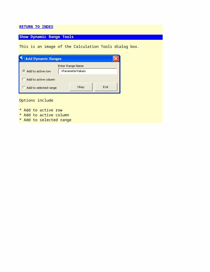
This is an image of the Export as Image File dialog box.

Export an image file of the selected range or autoshape. Choose between GIF, JPG or PNG.

You can also select between Bitmap and Picture formats.

The Bitmap is generally clearer, but the Picture type may be better if the image is resized.

RETURN TO INDEX

Export an image file of the selected range or autoshape. Choose between GIF, JPG or PNG.

The Bitmap is generally clearer, but the Picture type may be better if the image is resized.

Copy Picture Of Selection

This is a quick and simple way to copy a picture as a bitmap to the clipboard.

The image may then be pasted to another type of software such as an Graphics Editor.

Note: Not all Graphics Editors requires use of this tool, some do and some don't.

If you use it within Office software, including Excel, you will be copying a picture of a range or autoshape etc, not the range or autoshape itself.

RETURN TO INDEX

If you use it within Office software, including Excel, you will be copying a picture of a range or autoshape etc, not the range or autoshape itself.

Export Range As Text File

This is an image of the Export Range As Text File dialog box.

You can save a range as a text file, showing cell contents as either values or formulas.

These are the text file options.

1. CSV File2. Tab Delimited3. Space4. Other (Input a separator as required)

You can also show the text file automatically when finished.

RETURN TO INDEX

Show Checkbox Tools

This is an image of the Checkbox Tools dialog box.

There are 3 tools that you can use.

1. Add Checkboxes (Formatted to change color when ticked)Existing Conditional Formatting and cell text will be deleted

2. Tick Checkboxes(Forms Toolbar type checkboxes only)

3. Untick Checkboxes(Forms Toolbar type checkboxes only)

In the case of Tick Checkboxes and Untick Checkboxes, you can choose from the following.

1. Selection (Range currently selected)2. Sheet (Active Sheet)2. Book (Active Workbook)

RETURN TO INDEX

In the case of Tick Checkboxes and Untick Checkboxes, you can choose from the following.

Compare Cells

This is an image of the Compare Cells dialog box.

Compare 2 ranges to count unique and duplicate values by selecting ranges and pushing Update List.

Note: This utility is not available with Excel 97

RETURN TO INDEX

Compare 2 ranges to count unique and duplicate values by selecting ranges and pushing Update List.

Add Data Labels From Range

This is an image of the Chart Data Labeler dialog box.

Select a series and a range to copy values (with formats), fill and font colors as per the selected cells.

Not all charts offer all label positions shown in the drop down box. If not available, the default will be used.

RETURN TO INDEX

Select a series and a range to copy values (with formats), fill and font colors as per the selected cells.

Not all charts offer all label positions shown in the drop down box. If not available, the default will be used.

Change Series Colors From Range

This is an image of the Change Chart Series Colors dialog box.

Select a series and a range to color the series as per the selected cell's fill colors.

RETURN TO INDEX

Move Data Labels To Left

This is an image of the Move Data Labels To Left dialog box.

Select a series and the data labels will be moved to the left on top of each other.

Hint: Try it with a pie chart so all data labels can be seen.

RETURN TO INDEX

Maxe X Axis Cross At Minimum Value

Use this to make the X Axis of the active chart cross at the minimum value.

RETURN TO INDEX

Show Text And Format Tools

Tab 1. Add & Delete

Choose one of the following options from the drop down list.

These options will add or delete values in selected cells.

1. Remove NumbersFor example, A1B2C3D4 will become ABCD

2. Remove TextFor example, A1B2C3D4 will become 1234

3. Remove Excess SpacesFor example, "Text And Number Utilities" becomes "Text And Number Utilities"

4. Remove All SpacesFor example, "Text And Number Utilities" becomes "TextAndNumberUtilities"

5. Remove From Set Position* entering 3 and choosing First Characters will result in 1234567890 becoming 4567890 (First 3 characters are removed)* entering 3 and choosing Last Characters will result in 1234567890 becoming 1234567 (Last 3 characters are removed)* entering 3 and choosing Nth Character will result in 1234567890 becoming 123 (All after the first 3 characters is removed)

6. Remove Certain CharactersEnter the characters to be deleted into the appropiate text box (Case Sensitive)

RETURN TO INDEX

7. Add Text To Existing Text* If First Characters is selected, adding "ABC" to "0123456789" will result in "ABC0123456789"* If Last Characters is selected, adding "ABC" to "0123456789" will result in "0123456789ABC"

8. Add Single Fill Characters* If First Characters is selected, adding "*" to "ABC" wil become "*****ABC"* If Last Characters is selected, adding "*" to "ABC" wil become "ABC*****"Note: The number of fill characters that appear depends on the width of the cells

9. Add Repeat Fill Characters* If First Characters is selected, entering 3 for "How Many Times To Repeat", and adding "01" to "ABC" wil become "010101ABC"* If Last Characters is selected, entering 3 for "How Many Times To Repeat", and adding "01" to "ABC" wil become "ABC010101"

10. Add Superscript* With First Characters, entering 2 for "Enter Start Position", and 4 for "How Many Characters?" will result in the 2nd, 3rd, 4th and 5th characters becoming superscript* With Last Characters, entering 2 for "Enter Start Position"will result in the final 2 characters becoming superscript

11. Add Subscript* With First Characters, entering 2 for "Enter Start Position", and 4 for "How Many Characters?" will result in the 2nd, 3rd, 4th and 5th characters becoming subscript* With Last Characters, entering 2 for "Enter Start Position"will result in the final 2 characters becoming subscript

Push Okay when ready.

Tab 2. Format & Case

You can choose one of the following formats from the drop down list.

1. General2. Numeric3. Twin Decimal

4. Text5. dd/mm/yyd = Days, m = Months, y = Years

6. mm/dd/yyd = Days, m = Months, y = Years

7. yy/mm/ddd = Days, m = Months, y = Years

8. dd-mm-yyd = Days, m = Months, y = Years

9. mm-dd-yyd = Days, m = Months, y = Years

10. yy-mm-ddd = Days, m = Months, y = Years

11. d mmmm, yyyyd = Days, m = Months, y = Years

12. mmmm d, yyyyd = Days, m = Months, y = Years

13. yyyy-mm-dd (ISO)d = Days, m = Months, y = Years

14. h:mm (24 hrs)h = Hours, m = Minutes, s = Seconds

15. h:mm AM/PMh = Hours, m = Minutes, s = Seconds

16. h:mm:ss (24 hrs)h = Hours, m = Minutes, s = Seconds

17. h:mm:ss AM/PMh = Hours, m = Minutes, s = Seconds

18. hh:mm:ss (ISO)h = Hours, m = Minutes, s = Seconds

19. Upper Case20. Lower Case21. Proper Case

Or push one of these buttons,

1. Currency Format* Enter Currency Type (Type in a currency symbol or abbreviation if desired)* Enter Decimal Places (Type in a number of decimal places if desired)

2. Set Digits LengthFor example, entering 3 will result in 1 appearing as 001 and 11 appearing as 011 etc

You can also add or subtract Years, Months and Days to dates. (Use negative numbers to subtract)

Push Okay when ready to format or change dates.

Back to Top

* entering 3 and choosing First Characters will result in 1234567890 becoming 4567890 (First 3 characters are removed)* entering 3 and choosing Last Characters will result in 1234567890 becoming 1234567 (Last 3 characters are removed)* entering 3 and choosing Nth Character will result in 1234567890 becoming 123 (All after the first 3 characters is removed)

* If First Characters is selected, adding "ABC" to "0123456789" will result in "ABC0123456789"* If Last Characters is selected, adding "ABC" to "0123456789" will result in "0123456789ABC"

* If First Characters is selected, entering 3 for "How Many Times To Repeat", and adding "01" to "ABC" wil become "010101ABC"* If Last Characters is selected, entering 3 for "How Many Times To Repeat", and adding "01" to "ABC" wil become "ABC010101"

* With First Characters, entering 2 for "Enter Start Position", and 4 for "How Many Characters?" will result in the 2nd, 3rd, 4th and 5th characters becoming superscript* With Last Characters, entering 2 for "Enter Start Position"will result in the final 2 characters becoming superscript

* With First Characters, entering 2 for "Enter Start Position", and 4 for "How Many Characters?" will result in the 2nd, 3rd, 4th and 5th characters becoming subscript* With Last Characters, entering 2 for "Enter Start Position"will result in the final 2 characters becoming subscript

You can also add or subtract Years, Months and Days to dates. (Use negative numbers to subtract)

Replace Text Tools

This is an image of the Replace Text Tools dialog box.

There are 4 options.

1. Replace TextThis works in the same way as the SUBSTITUTE function in Excel.

2. Remove Text From LeftRemove all text from the left of a specified character (or first letter in a string)An option exists to include the character, works well with parsing names etc.

3. Remove Text From RightRemove all text from the right of a specified character (or first letter in a string)An option exists to include the character, works well with parsing names etc.

4. Remove Text From MiddleThis works in the same way as the REPLACE function in Excel.

RETURN TO INDEX

Insert Sequential List In Selection

This is an image of the List Utilities dialog box.

These are the different kinds of list options.

1. Sequential NumbersEnter a start number and an increment number. An optional prefix and suffix can be added to each number

2. Unique NumbersChoose a start number and non-repeating random numbers will be added to each cell in your selection

3. Repeating NumbersEnter Maximum and Minimum numbers for repeating random numbers

4. Capital Letters5. Small Letters6. Sequential DatesEnter a Start Year, Start Month, Start Day and increment number

Insert the list by pushing either of the List in Rows or List in Columns buttons.

RETURN TO INDEX

Enter a start number and an increment number. An optional prefix and suffix can be added to each number

Choose a start number and non-repeating random numbers will be added to each cell in your selection

Find Maximum And Minimum Values

This is an image of the Maximum And Minimum dialog box.

You can search for Maximum or Minimums within the selected range or active sheet.

Options to search can be specified to Values, Formulas and both Values and Formulas.

RETURN TO INDEX

Insert Bar Graph In Selection

This a quick and simple way to enter a bar graph into selected cells.

The color of the graph is optional. Other formatting can be done by selecting the graph, right-clicking and choosing "Format Autoshapes".

Note: If there is a very large difference between the values, only bars for the higher values may show. This is due to limitations of sizing the autoshapes.

RETURN TO INDEX

The color of the graph is optional. Other formatting can be done by selecting the graph, right-clicking and choosing "Format Autoshapes".

Note: If there is a very large difference between the values, only bars for the higher values may show. This is due to limitations of sizing the autoshapes.

Convert Numbers To Text (Add ' Mark)

Add a single quotation mark to numbers as in '123.

This enables you to work with these numbers as text.

RETURN TO INDEX

Revert Text Numbers To Real Numbers

This reverts numbers formatted as text back to normal numbers.

RETURN TO INDEX

Move Minus Sign To Front

For example, 123- will become -123. This may be useful for imported text.

RETURN TO INDEX

Positive And Negative Numbers

This is an image of the Positive And Negative Numbers dialog box.


1. Positive Numbers To Negative NumbersNegative numbers remain unchanged.

2. Negative Numbers To Positive NumbersPositive numbers remain unchanged.

3. Positive Numbers To ZerosNegative numbers remain unchanged..

4. Negative Numbers To ZerosPositive numbers remain unchanged.

5. Positive Numbers <-> Negative NumbersSwap Positive And Negative Numbers.

RETURN TO INDEX

Perform Quick Math On Selection

This is an image of the Quick Math dialog box.

Select an operator, enter a number and push Okay.

For example, if you choose Multiply, then enter the number 2, each numeric value in the selection will double.

You can choose to retain formulas or paste as values.

RETURN TO INDEX

For example, if you choose Multiply, then enter the number 2, each numeric value in the selection will double.

Round Numbers In Selection

This is an image of the Round Numbers dialog box.

These are the different kinds of rounding options.An input box will appear to enter a specified number of digits for the first 3 options

1. Round NumbersFor example, rounding off to 5 means 0.123454 results in 0.12345 and 0.123456 results in 0.12346For example, rounding off to -2 means 140 results in 100 and 160 results in 200

2. Round Numbers UpFor example, rounding off to 5 means both 0.123454 and 0.123456 results in 0.12346For example, rounding off to -2 means both 140 and 160 results in 200

3. Round Numbers DownFor example, rounding off to 5 means both 0.123454 and 0.123456 results in 0.12345For example, rounding off to -2 means both 140 and 160 results in 100

4. Remove DecimalsFor example, 1.23 becomes 1, 123.456 becomes 123

5. Remove IntegersFor example, 1.23 becomes 0.23, 123.456 becomes 0.456

RETURN TO INDEX

For example, rounding off to 5 means 0.123454 results in 0.12345 and 0.123456 results in 0.12346

Copy Sum Of Selection To Clipboard

Add numbers in a selection and copy the sum to the clipboard.

You can paste the total within Excel or other aplications.

RETURN TO INDEX

Delete Duplicates In Selection

Delete entire rows or columns with duplicates except where the first occurring values are found.

You must select one row (Delete Duplicates In Columns) or one column (Delete Duplicates In Rows) only.

Note: If you want to delete all duplicates, go to Sheet Utilities, Show Selection Tools, Selection Tools,then select Duplicates, Delete and then Entire Rows or Entire Columns as wanted.

You can also choose Cells, Select and then delete from the right click menu.

RETURN TO INDEX

Delete entire rows or columns with duplicates except where the first occurring values are found.

You must select one row (Delete Duplicates In Columns) or one column (Delete Duplicates In Rows) only.

Note: If you want to delete all duplicates, go to Sheet Utilities, Show Selection Tools, Selection Tools,

Show Conversion Tools

Choose one of the following to convert values in your selection.

1. Inches To Centimeters2. Feet To Meters3. Feet To Kilometers4. Yards To Meters5. Yards To Kilometers6. Yards To Miles7. Yards To Nautical Miles8. Millimeters To Inches9. Centimeters To Inches10. Meters To Feet11. Meters To Yards12. Meters To Miles13. Meters To Nautical Miles14. Sq Feet To Sq Meters15. Sq Yards To Acres16. Acres To Hectares17. Sq Meters To Sq Feet18. Sq Meters To Hectares19. Hectares To Acres20. Grams To Ounces21. Grams To Pounds22. Kilograms To Pounds23. Ounces To Pounds24. Ounces To Kilograms25. Pounds To Kilograms26. Pounds To Ounces27. Celsius To Fahrenheit28. Fahrenheit to Celsius

RETURN TO INDEX

Show Excel Calculator

This is an image of the Excel Calculator.

Use it like a normal calculator but this one is especially designed for Excel.

You can insert numbers from cells to the display, paste from the display to cells or copy from the display to the clipboard.

This total can then be pasted within Excel or other applications.

Note: Hover the mouse over the display to current totals.

RETURN TO INDEX

You can insert numbers from cells to the display, paste from the display to cells or copy from the display to the clipboard.

Show Special Characters

Display the Window's Character Map to select and copy special characters.

RETURN TO INDEX

Join Cell Text

This is an image of the Join Cell Text dialog box.

Select a Range and choose from one of the following options.

1. Joined Text In All CellsThe text in selected cells will be joined together and placed in all cellsFor example, if you have selected 3 cells and the values are 1, 2 and 3, then "123" will be placed in each selected cell

2. Joined Text In First CellThe text in selected cells will be joined together and placed in the first cellFor example, if you have selected 3 cells and the values are 1, 2 and 3, the result will become "123"Note: All other cells will be blank (the exisiting values will be deleted)

3. Joined Text In First RowAll text in selected cells below the first row will be added to cells in the first rowYou can add separators between the text of different cells as well as line breaksThere is also an option to clear cells below the first row after after the text has been joined

4. Joined Text In First ColumnAll text in selected cells below the first row will be added to cells in the first columnYou can add separators between the text of different cells as well as line breaksThere is also an option to clear cells below the first column after after the text has been joined

5. Copy Joined Text To ClipboardThe text in selected cells will be joined together and the result will be copied to the clipboardFor example, if you have selected 3 cells and the values are 1, 2 and 3, the result will become "123"

RETURN TO INDEX

You can also choose whether to add separators and/or line breaks between cell text.The joined text is copied to the clipboard but the text in the cells will remain unchanged

For example, if you have selected 3 cells and the values are 1, 2 and 3, then "123" will be placed in each selected cell

For example, if you have selected 3 cells and the values are 1, 2 and 3, the result will become "123"

There is also an option to clear cells below the first column after after the text has been joined

The text in selected cells will be joined together and the result will be copied to the clipboardFor example, if you have selected 3 cells and the values are 1, 2 and 3, the result will become "123"

Insert Multi Line Cell Text

This is an image of the Multi Line Cell Text dialog box.

You can add several lines of text to muliple cells at the same time.

An option to add the insert text to existing text in these cells is also available.

RETURN TO INDEX

Show Quick Write

This is an image of the Quick Write dialog box.

You can add values, text or even formulas so they can easily be entered into selected cells each and every time you use Excel. (They are stored between sessions in the registry)

If you enter the same things again and again, this really may save you a lot of valuable time.

EnterEnter the selected item into cells.

AddAdd new items. First add an entry (example, some text or a formula), then add a name (example, "Monthly Budget Totals Formula")

RenameYou can rename an item. (But you have to delete and re-add to change the value, text, formula itself)

DeleteDelete an item.

Move UpMove an item up.

Move Down

RETURN TO INDEX

Move an item down.

ExitExit Quick Write.

Note: Array formulas cannot be used.

Back to Top

You can add values, text or even formulas so they can easily be entered into selected cells each and every time you use Excel. (They are stored between sessions in the registry)

If you enter the same things again and again, this really may save you a lot of valuable time.

Add new items. First add an entry (example, some text or a formula), then add a name (example, "Monthly Budget Totals Formula")

You can rename an item. (But you have to delete and re-add to change the value, text, formula itself)

Show Excel Timer

This is an image of the Excel Timer dialog box.

You can choose to show a message or run a macro, once or repeatedly.

To run a macro, include the full workbook path and module name.

RETURN TO INDEX

Show Time Picker

This is an image of the Time Picker.

Push the Hours and (or) Minutes buttons as required.

For example,

If you push "1" for Hours, the value entered in cells will be one o'clock.

If you push, "05" for Minutes, the value entered will be 5 minutes past the hour.

If you push "1" and "05", the value will be 1:05.

Push the "Move to next cell" if required. If this is not selected within Excel (Tools, Options, Edit, Move selection after Enter) then the default direction will be down.

RETURN TO INDEX

Push the "Move to next cell" if required. If this is not selected within Excel (Tools, Options, Edit, Move selection after Enter) then the default direction will be down.

Insert Calendar Sheet

This is an image of the Insert Calendar Sheet dialog box.

Enter a year between 1901 and 3000, then choose from a Normal Calendar (weeks starts from Sundays)or an ISO Calendar (weeks start from Mondays, ISO Week Numbers and Day Numbers are also shown).

You can choose to add the sheet to the active workbook or to a new workbook.

RETURN TO INDEX

Enter a year between 1901 and 3000, then choose from a Normal Calendar (weeks starts from Sundays)or an ISO Calendar (weeks start from Mondays, ISO Week Numbers and Day Numbers are also shown).

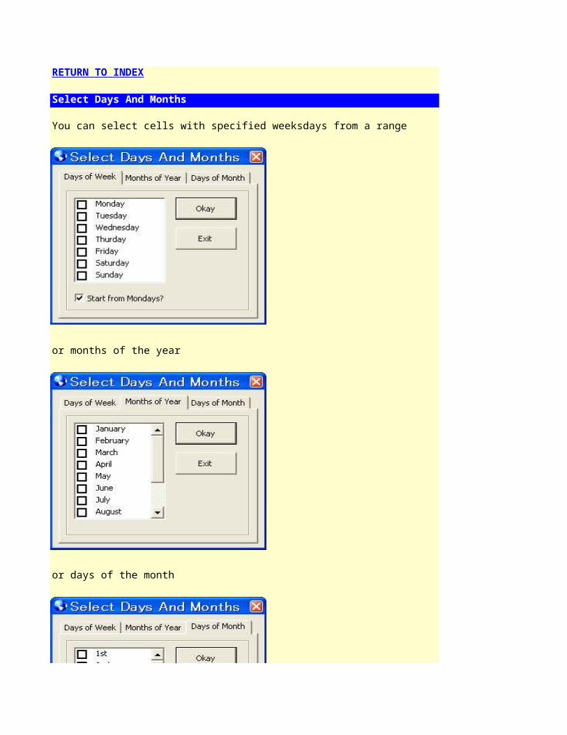
Select Days And Months

You can select cells with specified weeksdays from a range

or months of the year

or days of the month

RETURN TO INDEX

Show Calendar Date Picker

This is an image of the Excel Calendar Date Picker.

You can enter dates into cells by pushing the buttons that show the days of the month.

Use the spin buttons at the top to change the month (left side) or the year (right side).

You can also choose to start the weeks from Mondays.

Push the "Go to this month" button to return to the current month. The current day is highlighted when the current month is shown.

RETURN TO INDEX

Push the "Go to this month" button to return to the current month. The current day is highlighted when the current month is shown.

Change Excel Application Settings

Tab 1. Worksheet

1. Display Gridlines

2. Change Gridline ColorThe default for gridline colors is Automatic. With this setting, gridline colors will show as the grey lines you see whenever you open a new workbookNote that if you change the gridlines colors, the border colors will also change if they are set as Automatic too(The default color for borders is "black", but this is not really black, see below)

For example, blue gridlines means blue borders if the borders are set as Automatic. But if the borders are not set as Automatic, they will appearas the different color that you set them, (this includes "real" black) This allow you to have combinations gridlines and borders that are not the same color

At the same time, changing the gridlines back to Automatic results in the borders appearing "black" once again if they are set as Automatic tooTherefore if you if choose black for gridline colors with my Change Gridline Colors utility, you are asked whether you prefer black or Automatic

3. Display Pagebreaks

4. Display Row/Column Headers

5. Display Formulas

6. Display Zeroes

RETURN TO INDEX

Zoom Settings can be adjusted by either using an option button or the scroll bar.

You can also zoom to the current range using Fit to Selection.

Note: Push "Apply these settings to all sheets." for all sheets in the active book.

Tab 2. Workbook

1. Display Horizontal Scroll

2. Display Vertical Scroll

3. Display Worksheet Tabs

4. Show Full Name in Title Bar

Workbook Details

This shows the current file size, last save time and last user to edit the file of the active book when the dialog box is first displayed.

Note: This information will not show if the workbook is not yet saved.

Tab 3. Application

1. Display Formula Bar

2. Display Status Bar

3. Reset Status Bar

4. Calculation, Automatic or ManualYou can toggle to Manual Calculation to speed up working with Excel but keep the following in mind1. It affects all open workbooks2. If you save workbooks with this setting, it will affect all other files if these workbooks are the first files you open when using Excel later on3. Formulas will not be calculated automatically. You can push F9 to force calculation. (Use Shift + F9 for the active sheet only)

Note: This is a generally used as a temporary setting, you might want to turn Calculation back on before savingRemember distributed workbooks opened by others may also change their files to this setting. Use with due caution.

5. Reference, A1 Style or R1C1 StyleYou can toggle to R1C1 Style to see the Column numbers (rather than A, B, C etc) but keep the following in mind1. It affects all open workbooks2. If you save workbooks with this setting, it will affect all other files if these workbooks are the first files you open when using Excel later on


6. Enable Events, True or FalseYou can turn off Enable Events to prevent Event code from working but keep the following in mind1. It affects all open workbooks2. If you save workbooks with this setting, it will affect all other files if these workbooks are the first files you open when using Excel later on


Back to Top

The default for gridline colors is Automatic. With this setting, gridline colors will show as the grey lines you see whenever you open a new workbookNote that if you change the gridlines colors, the border colors will also change if they are set as Automatic too

For example, blue gridlines means blue borders if the borders are set as Automatic. But if the borders are not set as Automatic, they will appearas the different color that you set them, (this includes "real" black) This allow you to have combinations gridlines and borders that are not the same color

At the same time, changing the gridlines back to Automatic results in the borders appearing "black" once again if they are set as Automatic tooTherefore if you if choose black for gridline colors with my Change Gridline Colors utility, you are asked whether you prefer black or Automatic

This shows the current file size, last save time and last user to edit the file of the active book when the dialog box is first displayed.

You can toggle to Manual Calculation to speed up working with Excel but keep the following in mind

2. If you save workbooks with this setting, it will affect all other files if these workbooks are the first files you open when using Excel later on3. Formulas will not be calculated automatically. You can push F9 to force calculation. (Use Shift + F9 for the active sheet only)


You can toggle to R1C1 Style to see the Column numbers (rather than A, B, C etc) but keep the following in mind

2. If you save workbooks with this setting, it will affect all other files if these workbooks are the first files you open when using Excel later on


You can turn off Enable Events to prevent Event code from working but keep the following in mind

2. If you save workbooks with this setting, it will affect all other files if these workbooks are the first files you open when using Excel later on


Show Full Path And Book Name in Titlebar

Show the full path and name of the active workbook in the titlebar. This makes it easy to see where the workbook is saved.

RETURN TO INDEX

Show the full path and name of the active workbook in the titlebar. This makes it easy to see where the workbook is saved.

Copy Pathname To Clipboard

Copy the pathname of the active book to the clipboard. You can paste within Excel or other applications.

RETURN TO INDEX

Copy the pathname of the active book to the clipboard. You can paste within Excel or other applications.

Open Dialog Box With Current File's Folder

The Open Dialog Box will be shown with the current file's folder.

RETURN TO INDEX

Open Explorer With Current File's Folder

Explorer will be opened to the folder of the active file. Works on LAN also.

RETURN TO INDEX

Show Folder Details in Worksheet

This is an image of the Show Folder Details dialog box.

You can make a list of files within a folder (and subfolders) in a new worksheet or book.

Options to select files are as below.

1. All Files

2. Excel Files (.xls)

3. Other FilesEnter a file name or extension such as ".gif" to find files that meet that descriptionWildcards (*) can be used. Either upper or lower case can be used

You can add hyperlinks to open the files after they are shown in Excel. (Just click the links to do so)

Note: This utility does not work properly with Excel 97. (But the option to specify a File Name or Extension works fine)

RETURN TO INDEX

You can add hyperlinks to open the files after they are shown in Excel. (Just click the links to do so)

Note: This utility does not work properly with Excel 97. (But the option to specify a File Name or Extension works fine)

Add Workbook to Recent Files

Sometimes workbooks don't get added to your recent files list. This will do it for you.

RETURN TO INDEX

Clear Recent Files List

Clear your recent files list quickly.

RETURN TO INDEX

Rename Active Workbook While Open

This is a very useful way of renaming/relocating your files. You can also use it to make copies.

RETURN TO INDEX

This is a very useful way of renaming/relocating your files. You can also use it to make copies.

Delete Active Workbook While Open

Delete the active workbook while it is still open.

RETURN TO INDEX

Save Workbook With Backup File

This enables you to save a backup file of the active workbook.

RETURN TO INDEX

Reopen Workbook Without Saving

Reopen the active book quickly without prompts or having to locate the file in your recent files list.

RETURN TO INDEX

Reopen the active book quickly without prompts or having to locate the file in your recent files list.

Close Saved Workbooks

Close already saved workbooks without the need to check (only saved workbook are closed)

RETURN TO INDEX

Close already saved workbooks without the need to check (only saved workbook are closed)

Insert Headers And Footers

This is an image of the Insert Header/Footer dialog box.

Enter text in the text box provided and/or push one of the folllowing buttons to enter special text quickly.

* Full Name* File Name* Date* Time

Make sure to choose a header or footer option.

* Left Header* Center Header* Right Header* Left Footer* Center Footer* Right Footer

Other options included,

RETURN TO INDEX

* Change Header/Footer Font Style* Apply To All Sheets in Workbook* Clear Other Headers & Footers

Push Okay when ready.

Unless "Apply To All Sheets in Workbook" is ticked, the choices made will apply only to selected sheets.(Push Ctrl and the worksheet tabs at the bottom of Excel to select multiple sheets)

Note: To quickly clear all headers and footers, make sure text box is empty, then select any header or footer option (for example Left Header) then push Okay.This will include clearing the header or footer that is selected.

Back to Top

Enter text in the text box provided and/or push one of the folllowing buttons to enter special text quickly.

Unless "Apply To All Sheets in Workbook" is ticked, the choices made will apply only to selected sheets.

Note: To quickly clear all headers and footers, make sure text box is empty, then select any header or footer option (for example Left Header) then push Okay.

Show Active Workbook Details

The following details are shown.

Sheet Names and TypesBuiltIn PropertiesCustom PropertiesVBA Modules and code withinExcel Links (broken links shown in red)OLE LinksNames (includes Scope, Refers To and Visibility)

RETURN TO INDEX

Delete Active Workbook Macros

Delete all VBA code within the active workbook.

RETURN TO INDEX

Show Excel Menu Details

Add a worksheet or new workbook that shows Built-In Menu Details.

* Names

* IDs

* Menu Types

RETURN TO INDEX

Show Face IDs Toolbar

Show available Face IDs (button images) for your Excel version along with their ID numbers. (Hover the cursor above the Face IDs)

RETURN TO INDEX

Show available Face IDs (button images) for your Excel version along with their ID numbers. (Hover the cursor above the Face IDs)

Delete Custom Toolbars

This is an image of the Delete Custom Toolbars dialog box.

Use it to delete custom toolbars manually.

RETURN TO INDEX

Delete Custom Controls

This is an image of the Delete Custom Controls dialog box.

Use it to delete custom controls manually.

RETURN TO INDEX

Reset Tools

This is an image of the Reset Tools dialog box.

Tools include -

Reset CursorReset CalculationReset Display AlertsReset StatusbarReset EventsReset All (of the above)

RETURN TO INDEX

Show Excel Color Details

Add a worksheet or new workbook to show the following information.

* the Color Index

* the HTML Color

* the RGB Index

* the Color Name

RETURN TO INDEX

Show Color Picker

Show a dialog box with the following information for the active cell or shape.

* the Color Index

* the HTML Color

* the RGB Index

* the Color Name

If there is no fill color used, the Color Index and the Color Name will show as "Not Available".

RETURN TO INDEX

If there is no fill color used, the Color Index and the Color Name will show as "Not Available".

Web Search From Excel

This enables you to search the web directly from cells. (Flip between your browser and Excel by pushing Tab and Alt)

The following web searches are available.

* Google Web Search

* Google Image Search

* Dictionary.Com

* Thesaurus.com

* Wikipedia

* Encarta Maps

RETURN TO INDEX

This enables you to search the web directly from cells. (Flip between your browser and Excel by pushing Tab and Alt)

Play Mastermind

This is an image of the Mastermind Game.

Push the Help button to see the rules.

RETURN TO INDEX

Play Simon Says

This is an image of the Simon Says Game.

Select a speed and time, then push Start.

Watch the flashing squares, then the try to match them in the same order.

RETURN TO INDEX

Generate Password

This is an image of the Password Maker dialog box.

Select a number of characters and use non-standard (non-alphabetic symbols) if desired.

There is a button to copy the password to the clipboard.

RETURN TO INDEX

Add JMT Functions To Workbook

Add JMT Functions to the active workbook.

You can see more about the various functions available here.

RETURN TO INDEX

Custom Functions, How to use them

JMT Excel Utilities Settings

This is an image of the JMT Excel Utilities Settings dialog box.

Some basic system information is shown as well as the following options.

1. Select from the Main Menu, Right-Click Menu or Toolbar styles.

The utilities will be saved in the menu style you choose.

2. Resore JMT Excel Utilities Settings.

All settings will be restored to default values.

JMT Excel Utilities were brought to you by- Masaru Kaji aka Colo, Microsoft Excel MVP and owner of Colo's Excel Junk Room

- Andrew Engwirda, Excel Addict and owner of Andrew's Excel Tips

Together we operate the JMT Excel Consulting website.

RETURN TO INDEX

http://puremis.net/excel

http://www.andrewsexceltips.com/tips.htm

http://jmt.puremis.net

http://puremis.net/excel

http://www.andrewsexceltips.com/tips.htm

http://jmt.puremis.net/

Show JMT Help Files

Used to show these Help Files.

RETURN TO INDEX

Custom Functions, How to use them

Custom Functions can make life a lot easier but unlike in-built Excel functions like SUM or TODAY, there are some things to keep in mind when working with them.

1. They can be entered with either upper or lower text. But keep in mind that Excel will continue to show them in the same case as they are entered the first time.

2. Custom Functions must exist in all files that use them, otherwise they will show as a #NAME? error. If your files are used on several computers, you must install them in each one. To do this, use Add JMT Functions To Workbook from the Other Utilities menu.

3. Depending on your security settings, you may be asked to enable macros. This is normal and must be enabled each time so the custom functions can work.

RETURN TO INDEX

Custom Functions can make life a lot easier but unlike in-built Excel functions like SUM or TODAY, there are some things to keep in mind when working with them.

1. They can be entered with either upper or lower text. But keep in mind that Excel will continue to show them in the same case as they are entered the first time.

2. Custom Functions must exist in all files that use them, otherwise they will show as a #NAME? error. If your files are used on several computers, you must install them in each one.

3. Depending on your security settings, you may be asked to enable macros. This is normal and must be enabled each time so the custom functions can work.

2. Custom Functions must exist in all files that use them, otherwise they will show as a #NAME? error. If your files are used on several computers, you must install them in each one.

Custom Function Details

HASFORMULAReturns TRUE if Target Cell has formula

GETFORMULAReturns formula used in Target Cell

GETFORMATReturns format used in Target Cell

GETFONTReturns font name and size used in Target Cell

GETCOMMENTReturns text from comment in Target Cell

SHEETSNAMEReturns Active Sheet's name

BOOKSNAMEReturns Active Workbook's name

FULLNAMEReturns Active Workbook's full name (includes directory)

USERSNAMEReturns the user's name

PATHNAMEReturns Active Workbook's path

ROWSIZEReturns Row Height of Active Cell if no range (Target Cell) is specified

COLUMNSIZEReturns Column Width of Active Cell if no range (Target Cell) is specified

FIRSTINROWReturns the First Value in the row specified

FIRSTINCOLUMNReturns the First Value in the column specified

LASTINROWReturns the Last Value in the row specified

RETURN TO INDEX

LASTINCOLUMNReturns the Last Value in the column specified

MILLIONSRound numbers up to millions as in "10 Million", recommended maximum of 15 digits(A custom format of #,##0,, can also be used)

THOUSANDSRound numbers up to thousands as in "10 Thousand", recommended maximum of 12 digits(A custom format of #,##0, can also be used)

GETNUMBERSReturns numbers as string and retains leading zeros (all text is removed)Use double negative for real numbers as in --GetNumbers(Target Cell As Range)Leading zeros will be lost with real numbers unless formatted accordinglySee http://www.andrewsexceltips.com/menu_formats_zeros_front_numbers.htm

GETTEXTReturns capital or small letters only (all numbers are removed)

HASTEXTReturns TRUE if text or numbers in second Target Cell are contained in first Target Cell

REVERSETEXTReverses Text of Target Cell

MAKE PASSWORDReturns a random password based on number of characters and optional use of symbols

GETCOLORINDEXReturns the color index of the Target Cell. Use Optional CondFormat 1, 2 or 3 for Conditional Formatting.No Fill Color or "0" will show if there is no color.

GETFONTINDEXReturns the font color index of the Target Cell. Use Optional CondFormat 1, 2 or 3 for Conditional Formatting.Will not work with Number Formats

COLORNAMEReturns the color name of the Target Cell. Use Optional CondFormat 1, 2 or 3 for Conditional Formatting.A blank or #NA will show in the case of an error

GETHTMLCOLORReturns HTML Color of Target CellIt will not work with Conditional Formatting

GETRGBCOLORReturns RGB Color of Target Cell

It will not work with Conditional Formatting

COUNTCOLORCounts all cells of the color specified (ColorInd = Color Index)It will not work with Conditional Formatting

SUMCOLORSums values in all cells of the color specified (ColorInd = Color Index)It will not work with Conditional Formatting

DATEFORMATSelect a number to change format of Target Cell or decline to retain same format as Target Cell

Formats shown when entering a number for "Choose Format"

1 = "dd/mm/yy"2 = "mm/dd/yy"3 = "d mmmm, yyyy"4 = "mmmm d, yyyy"

For examples Cell A1 has the date 12/31/00, then =DATEFORMAT(A1,3) = 31 December, 2000

DATEFORMAT2Select a number to change format of TargetDate, can be used with TODAY, NOW or dates entered with commasFormatting is the same as with DATEFORMAT

EDATEPLUSWorks as an alternative to the EDATE function fron the Analysis Toolpak (good news if you don't have it installed)

EOMONTHPLUSWorks as an alternative to the EOMONTH function fron the Analysis Toolpak (good news if you don't have it installed)

LASTDATEReturns Last Date of a Month specified by MyDay (Sunday = 1, Monday = 2, Tuesday = 3 etc)

STATRANDReturns static random numbers (similar to RAND)

STATRANDBETWEENReturns static random numbers between values specified (similar to RANDBETWEEN)

CHAINConcatenates (Joins) numbers or text together, with or without separatorsSeparators must be enclosed by quotation marks as in "-" etc.

Back to Top

Round numbers up to thousands as in "10 Thousand", recommended maximum of 12 digits

Returns the color index of the Target Cell. Use Optional CondFormat 1, 2 or 3 for Conditional Formatting.

Returns the font color index of the Target Cell. Use Optional CondFormat 1, 2 or 3 for Conditional Formatting.

Returns the color name of the Target Cell. Use Optional CondFormat 1, 2 or 3 for Conditional Formatting.

Select a number to change format of Target Cell or decline to retain same format as Target Cell

For examples Cell A1 has the date 12/31/00, then =DATEFORMAT(A1,3) = 31 December, 2000

Select a number to change format of TargetDate, can be used with TODAY, NOW or dates entered with commas

Works as an alternative to the EDATE function fron the Analysis Toolpak (good news if you don't have it installed)

Works as an alternative to the EOMONTH function fron the Analysis Toolpak (good news if you don't have it installed)

Returns Last Date of a Month specified by MyDay (Sunday = 1, Monday = 2, Tuesday = 3 etc)

JMT Excel Utilities

Thank you for buying these utilities.

Some general advice -

1. When working with these utilities, keep in mind that a lot of them loop through cells, areas, sheets, etc. Therefore it may be in your best interests to narrow your selection as much as possible to reduce time for the code to complete. Avoid doing things like selecting entire columns unless you really have to - some of these utilies however are almost instantaneous.

2. When using them for the first time, it might be a good idea to test first to make sure the utilities are working as expected. We recommend you back up your work at regular intervals as a safety measure. That said, to the best of our knowlege, none of these utilities should create problems if used correctly. (Please see the disclaimer in our Read Me file)

We hope they come in useful. Please send any feedback or suggestions to our email address ([email protected])

RETURN TO INDEX



We hope they come in useful. Please send any feedback or suggestions to our email address ([email protected])






Documents

JMT Excel Utilities Help Files