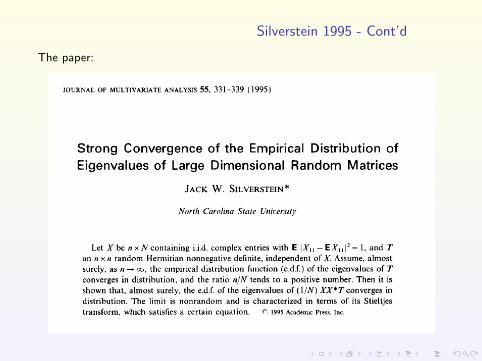
A note on a Marcenko-Pastur type theorem for time series

Jianfeng Yao

Workshop on High-dimensional statistics

The University of Hong Kong, October 2011

Overview

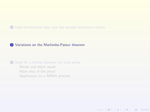
1 High-dimensional data and the sample covariance matrix

2 Variations on the Marcenko-Pastur theorem

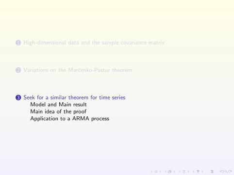
3 Seek for a similar theorem for time seriesModel and Main resultMain idea of the proofApplication to a ARMA process

1 High-dimensional data and the sample covariance matrix

2 Variations on the Marcenko-Pastur theorem

3 Seek for a similar theorem for time seriesModel and Main resultMain idea of the proofApplication to a ARMA process

The sample covariance matrix Sn

• Consider a sequence of p-dimensional random vectors, x1, . . . , xn withpopulation covariance matrix Σ = Cov(x1);

• The sample covariance matrix is

Sn =1

n

n∑j=1

xjxTj , or Sn =

1

n

n∑j=1

(xj − x)(xj − x)T .

• Classical theory: p is fixed and n→∞,

Sn → Σ, almost surely.

In particular, the p (random) eigenvalues of Sn

λSn1 ≥ · · · ≥ λ

Snp ,

converge to the eigenvalues of Σ.

High-dimensional data

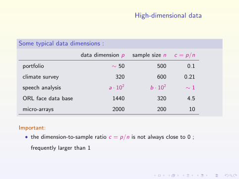
Some typical data dimensions :

data dimension p sample size n c = p/n

portfolio ∼ 50 500 0.1

climate survey 320 600 0.21

speech analysis a · 102 b · 102 ∼ 1

ORL face data base 1440 320 4.5

micro-arrays 2000 200 10

Important:

• the dimension-to-sample ratio c = p/n is not always close to 0 ;

frequently larger than 1

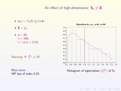
An effect of high-dimensions: Sn 6' Σ

• (xi ) ∼ Np(0, Ip) i.i.d.;

• Σ = Ip;

• p = 40,n = 160,c = p/n = 0.25.

Warning: !! λSnj 6= 1!!

Blue curve:MP law of index 0.25

0.2 0.4 0.6 0.8 1.0 1.2 1.4 1.6 1.8 2.0 2.2 2.4

0.0

0.1

0.2

0.3

0.4

0.5

0.6

0.7

0.8

0.9

1.0

Répartition des v.p., p=40, n=160

Histogram of eigenvalues {λSnj } of Sn

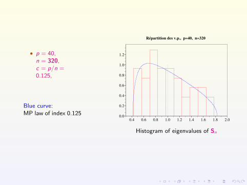
• p = 40,n = 320,c = p/n =0.125,

Blue curve:MP law of index 0.125

0.4 0.6 0.8 1.0 1.2 1.4 1.6 1.8 2.0

0.0

0.2

0.4

0.6

0.8

1.0

1.2

Répartition des v.p., p=40, n=320

Histogram of eigenvalues of Sn

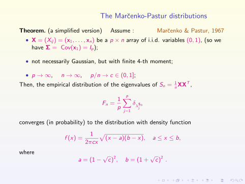
The Marcenko-Pastur distributions

Theorem. (a simplified version) Assume : Marcenko & Pastur, 1967

• X = (Xij) = (x1, . . . , xn) be a p × n array of i.i.d. variables (0, 1), (so wehave Σ = Cov(x1) = Ip);

• not necessarily Gaussian, but with finite 4-th moment;

• p →∞, n→∞, p/n→ c ∈ (0, 1];

Then, the empirical distribution of the eigenvalues of Sn = 1nXXT ,

Fn =1

p

p∑j=1

δλ

Snj

converges (in probability) to the distribution with density function

f (x) =1

2πcx

√(x − a)(b − x), a ≤ x ≤ b,

wherea = (1−

√c)2, b = (1 +

√c)2 .

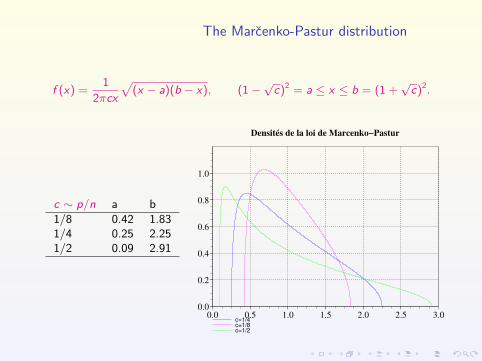
The Marcenko-Pastur distribution

f (x) =1

2πcx

√(x − a)(b − x), (1−

√c)2 = a ≤ x ≤ b = (1 +

√c)2.

c ∼ p/n a b1/8 0.42 1.831/4 0.25 2.251/2 0.09 2.91

c=1/4c=1/8c=1/2

0.0 0.5 1.0 1.5 2.0 2.5 3.0

0.0

0.2

0.4

0.6

0.8

1.0

Densités de la loi de Marcenko−Pastur

1 High-dimensional data and the sample covariance matrix

2 Variations on the Marcenko-Pastur theorem

3 Seek for a similar theorem for time seriesModel and Main resultMain idea of the proofApplication to a ARMA process

• Marcenko-Pastur’s original version;

• Silverstein 1995’s version;

• Bai and Zhou 2008’s version.

Marcenko-Pastur 1967

�������������������������8VERWPEXIH�ERH�TYFPMWLIH�F]�%17������

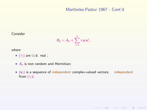
Marcenko-Pastur 1967 - Cont’d

Consider

Bp = Ap +n∑

i=1

τixix∗i ,

where

• (τi ) are i.i.d. real ;

• Ap is non random and Hermitian;

• (xi ) is a sequence of independent complex-valued vectors; independentfrom (τi );

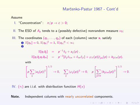
Marcenko-Pastur 1967 - Cont’d

Assume

I. “Concentration”: n/p → c > 0;

II. The ESD of Ap tends to a (possibly defective) nonrandom measure ν0;

III. The coordinates (q1, . . . , qp) of each (column) vector xi satisfy

1 E[qk ] = 0, E|qk |2 = 1, E|qk |4 <∞;2

E[qi qj ] = p−1δij + aij (p) ,

E[qi qjq`qm] = p−2[δijδ`m + δimδj`] + ϕi`(p)ϕjm(p) + bij`m(p),

withp∑ij

|aij (p)|21/2

→ 0,∑ij

|ϕij (p)|2 → 0, p

∑ij`m

|bij`m(p)|21/2

→ 0.

IV. (τi ) are i.i.d. with distribution function H(x)

Note. Independent columns with nearly uncorrelated components.

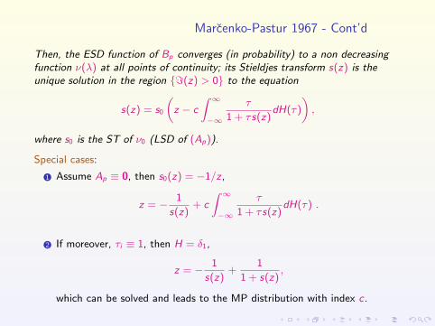
Marcenko-Pastur 1967 - Cont’d

Then, the ESD function of Bp converges (in probability) to a non decreasingfunction ν(λ) at all points of continuity; its Stieldjes transform s(z) is theunique solution in the region {=(z) > 0} to the equation

s(z) = s0

(z − c

∫ ∞−∞

τ

1 + τs(z)dH(τ)

),

where s0 is the ST of ν0 (LSD of (Ap)).

Special cases:

1 Assume Ap ≡ 0, then s0(z) = −1/z ,

z = − 1

s(z)+ c

∫ ∞−∞

τ

1 + τs(z)dH(τ) .

2 If moreover, τi ≡ 1, then H = δ1,

z = − 1

s(z)+

1

1 + s(z),

which can be solved and leads to the MP distribution with index c.

Silverstein 1995

The paper in MathScinet:

Silverstein 1995 - Cont’d

The paper:

Silverstein 1995’s theorem

And the theorem:

Silverstein versus Marcenko-Pastur

Silverstein:

• Write Xn = (x1, . . . , xN) and set yj = T1/2n xj , then Silverstein’s matrix Bn

is

Bn =1

NT 1/2

n XnX ∗n T 1/2n =

1

N

N∑j=1

yjy∗j ,

i.e. the SCM of i.i.d. random vectors (yj) with a special structure;=⇒: more general correlations Tn within the coordinates

• The convergence of the ESD is stronger (almost sure);

• Matrix entries are square-integrable only.

Marcenko-Pastur:

• The final equations appeared already in Marcenko-Pastur; also thosematrices have an extra additional term An. (Note however there is a similarpaper by Silverstein and Bai where this additional matrix An is present).

Yet another MP type theorem

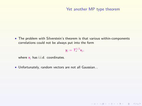
• The problem with Silverstein’s theorem is that various within-componentscorrelations could not be always put into the form

yj = T 1/2n xj ,

where xj has i.i.d. coordinates.

• Unfortunately, random vectors are not all Gaussian...

Bai and Zhou 2008’ theorem

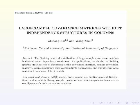
Note. Independent columns; and 1). specifies a very general correlationpattern within the components.

1 High-dimensional data and the sample covariance matrix

2 Variations on the Marcenko-Pastur theorem

3 Seek for a similar theorem for time seriesModel and Main resultMain idea of the proofApplication to a ARMA process

What’s next ?

• What about dependent columns, for example a p-dimensional time series,x1, . . . , xn, with stationary population covariance matrix Σ = Cov(xt) ?

• The problem is open for linear time series with general Σ.

• A solution below for linear time series with Σ = Ip.

An example

• SP 500 daily stock prices ; p = 488 stocks;

• n = 1000 daily returns rt(i) = log pt(i)/pt−1(i) from 2007-09-24 to2011-09-12;

The sample correlation matrix

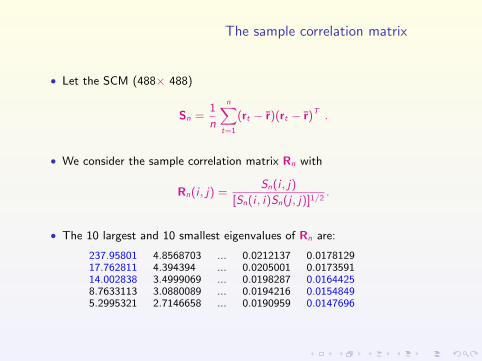
• Let the SCM (488× 488)

Sn =1

n

n∑t=1

(rt − r)(rt − r)T .

• We consider the sample correlation matrix Rn with

Rn(i , j) =Sn(i , j)

[Sn(i , i)Sn(j , j)]1/2.

• The 10 largest and 10 smallest eigenvalues of Rn are:

237.95801 4.8568703 ... 0.0212137 0.017812917.762811 4.394394 ... 0.0205001 0.017359114.002838 3.4999069 ... 0.0198287 0.01644258.7633113 3.0880089 ... 0.0194216 0.01548495.2995321 2.7146658 ... 0.0190959 0.0147696

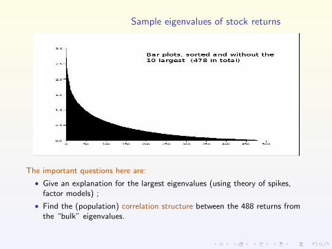
Sample eigenvalues of stock returns

The important questions here are:

• Give an explanation for the largest eigenvalues (using theory of spikes,factor models) ;

• Find the (population) correlation structure between the 488 returns fromthe “bulk” eigenvalues.

A Marcenko-Pastur type theorem for time series

• A very special case of time series;

• The ST of the LSD characterised by an equation depending on thespectral density of the time series.

The model

• consider an univariate real-valued linear process

zt =∞∑k=0

φkεt−k , t ∈ Z, (1)

where (εk) is a real-valued i. i. d. noise with mean zero and variance 1.

• The p-dimensional process (Xt) considered in this paper will be made by pindependent copies of the linear process (zt), i.e. for Xt = (X1t , . . . ,Xpt)

>,

Xit =∞∑k=0

φkεi,t−k , t ∈ Z,

where the p coordinate processes {(ε1,t , . . . , εp,t)} are independent copiesof the univariate error process {εt} in (1).

The SCM Sn

• Let X1, . . . ,Xn be the observations of the time series;

• we consider the ESD of the SCM

Sn =1

n

n∑j=1

XjX>j . (2)

Note. A previous paper by Jing at al. (2009) considers a similar question, butour result here is much more general (although not enough!).

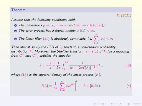
Theorem

Y. (2011)Assume that the following conditions hold:

1 The dimensions p →∞, n→∞ and p/n→ c ∈ (0,∞);

2 The error process has a fourth moment: Eε4t <∞;

3 The linear filter (φk) is absolutely summable, i.e.∞∑k=0

|φk | <∞.

Then almost surely the ESD of Sn tends to a non-random probabilitydistribution F . Moreover, the Stieltjes transform s = s(z) of F (as a mappingfrom C+ into C+) satisfies the equation

z = −1

s+

1

2π

∫ 2π

0

1

cs + {2πf (λ)}−1dλ , (3)

where f (λ) is the spectral density of the linear process (zt):

f (λ) =1

2π

∣∣∣∣∣∞∑k=0

φke ikλ

∣∣∣∣∣2

, λ ∈ [0, 2π). (4)

Main idea of the proof

• The data matrix (X1, . . . ,Xn) have p i.i.d. rows;

• the correlations in a row are the autocovariances of the base linear process(zt): for all 1 ≤ i ≤ p,

Cov(Xis ,Xit) = Cov(zs , zt) = γt−s , 1 ≤ s, t ≤ n .

• We can then adapt Bai and Zhou’s theorem to this case with an evaluationof these autocovariances and exchanging the roles of columns/rows.

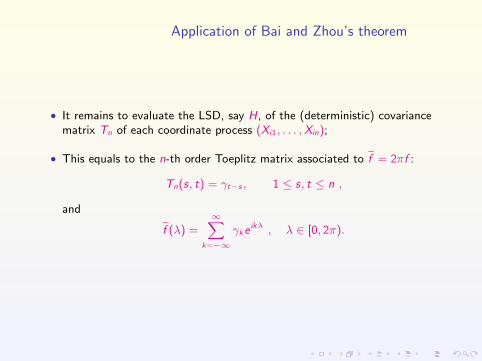
Application of Bai and Zhou’s theorem

• It remains to evaluate the LSD, say H, of the (deterministic) covariancematrix Tn of each coordinate process (Xi1, . . . ,Xin);

• This equals to the n-th order Toeplitz matrix associated to f = 2πf :

Tn(s, t) = γt−s , 1 ≤ s, t ≤ n ,

and

f (λ) =∞∑

k=−∞

γke ikλ , λ ∈ [0, 2π).

Cont’d

Assume that we can apply Bai and Zhou’s theorem:

• first we identify the ESD H of the Toeplitz matrices Tn;

• second, the ESD of np

Sn converges a.s nonrandom probability distributionwhose Stieltjes transform m solves the equation

z = − 1

m+

1

c

∫x

1 + mxdH(x).

• Need a theorem from Gabor Szego to compute the last integral.

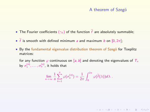
A theorem of Szego

• The Fourier coefficients (γk) of the function f are absolutely summable;

• f is smooth with defined minimum a and maximum b on [0, 2π];

• By the fundamental eigenvalue distribution theorem of Szego for Toeplitzmatrices:

for any function ϕ continuous on [a, b] and denoting the eigenvalues of Tn

by σ(n)1 , . . . , σ

(n)n , it holds that

limn→∞

1

n

n∑k=1

ϕ(σ(n)k ) =

1

2π

∫ 2π

0

ϕ(f (λ))dλ .

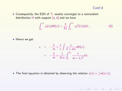
Cont’d

• Consequently, the ESD of Tn weakly converges to a nonrandomdistribution H with support [a, b] and we have∫ ∞

0

ϕ(x)dH(x) =1

2π

∫ 2π

0

ϕ(f (λ))dλ . (5)

• Hence we get

z = − 1

m+

1

c

∫x

1 + mxdH(x)

= − 1

m+

1

2πc

∫ 2π

0

1

m + 1/fdλ .

• The final equation is obtained by observing the relation s(z) = 1c

m(z/c).

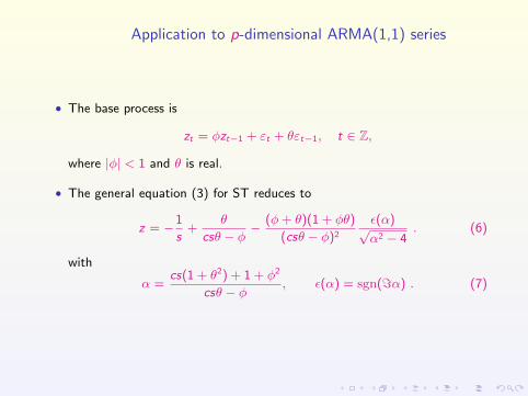
Application to p-dimensional ARMA(1,1) series

• The base process is

zt = φzt−1 + εt + θεt−1, t ∈ Z,

where |φ| < 1 and θ is real.

• The general equation (3) for ST reduces to

z = −1

s+

θ

csθ − φ −(φ+ θ)(1 + φθ)

(csθ − φ)2

ε(α)√α2 − 4

. (6)

with

α =cs(1 + θ2) + 1 + φ2

csθ − φ , ε(α) = sgn(=α) . (7)

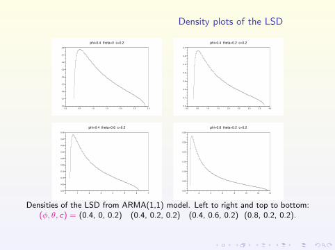
Density plots of the LSD

0.0 0.5 1.0 1.5 2.0 2.5 3.0

0.0

0.1

0.2

0.3

0.4

0.5

0.6

0.7

0.8

phi=0.4 theta=0 c=0.2

0.0 0.5 1.0 1.5 2.0 2.5 3.0 3.5 4.0

0.0

0.1

0.2

0.3

0.4

0.5

0.6

0.7

phi=0.4 theta=0.2 c=0.2

0 1 2 3 4 5 6 7

0.00

0.05

0.10

0.15

0.20

0.25

0.30

0.35

0.40

0.45

phi=0.4 theta=0.6 c=0.2

0 2 4 6 8 10 12 14

0.00

0.05

0.10

0.15

0.20

0.25

0.30

phi=0.8 theta=0.2 c=0.2

Densities of the LSD from ARMA(1,1) model. Left to right and top to bottom:(φ, θ, c) = (0.4, 0, 0.2) (0.4, 0.2, 0.2) (0.4, 0.6, 0.2) (0.8, 0.2, 0.2).

Conclusions

• Marcenko-Pastur theorems are a fundamental tool for the understandingof the spectral distributions of large sample covariance matrices;

• For dependent observations (time series for example), much work need tobe done; existing results are partial answers only.