Embed Size (px)
Citation preview
Inflationary CosmologyInflationary Cosmology
Jerome Martin
CNRS/Institut d’Astrophysique de
Paris
Jose Plinio Baptista School of Cosmology
March 9-14, 2014
2
Outline
Four Lectures
Lecture I: The Problems of the Hot Big Bang Model
Lecture II: The Inflationary Solution
Lecture III: Inflationary Perturbations of Quantum-Mechanical Origin
Lecture IV: Inflation and Planck

3
Lecture I
Lecture I: problems of the standard hot Big Bang model
4
The « hot Big Bang phase » is the standard cosmological model and provides a convincing description of the Universe on a wide range of energy scales.
The model is based on three assumptions:
1- Gravity is described by General Relativity
2- Cosmological principle: the Universe is homogeneous and isotropic (on large scales)
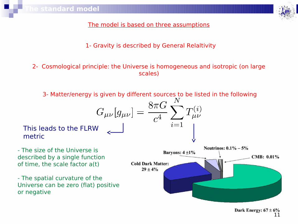
3- Matter/energy is given by different sources to be listed in the following
The standard model

5
The standard model
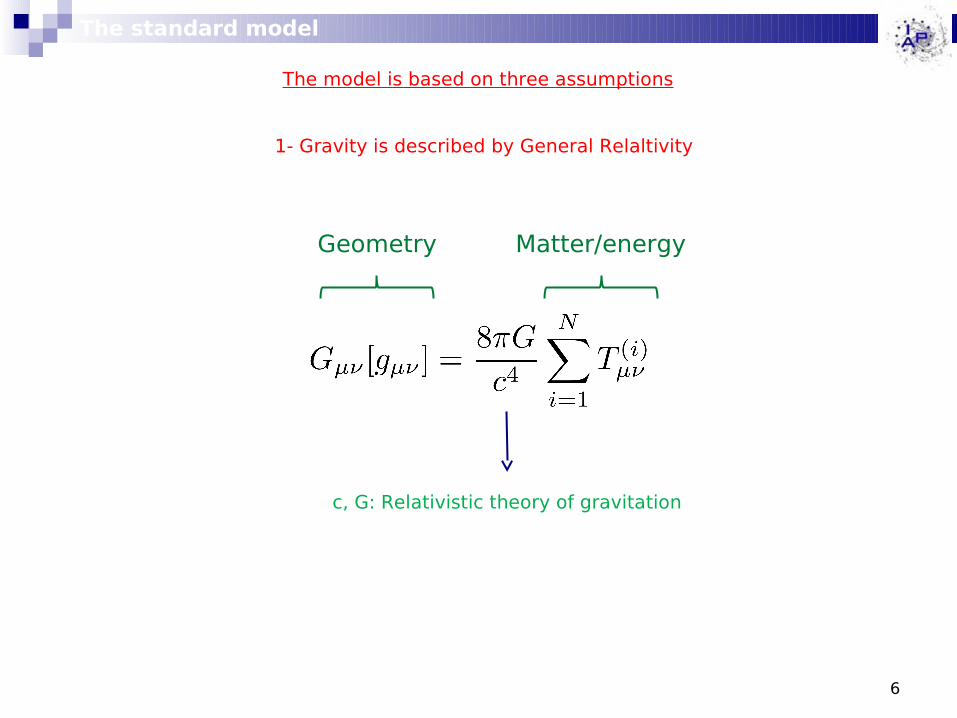
The model is based on three assumptions
6
The standard model
The model is based on three assumptions
1- Gravity is described by General Relaltivity
c, G: Relativistic theory of gravitation
Geometry Matter/energy
7
The standard model
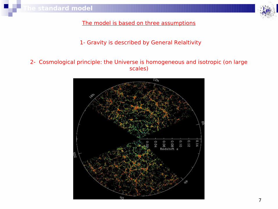
The model is based on three assumptions
1- Gravity is described by General Relaltivity
2- Cosmological principle: the Universe is homogeneous and isotropic (on large scales)

8
The standard model
The model is based on three assumptions
1- Gravity is described by General Relaltivity
2- Cosmological principle: the Universe is homogeneous and isotropic (on large scales)
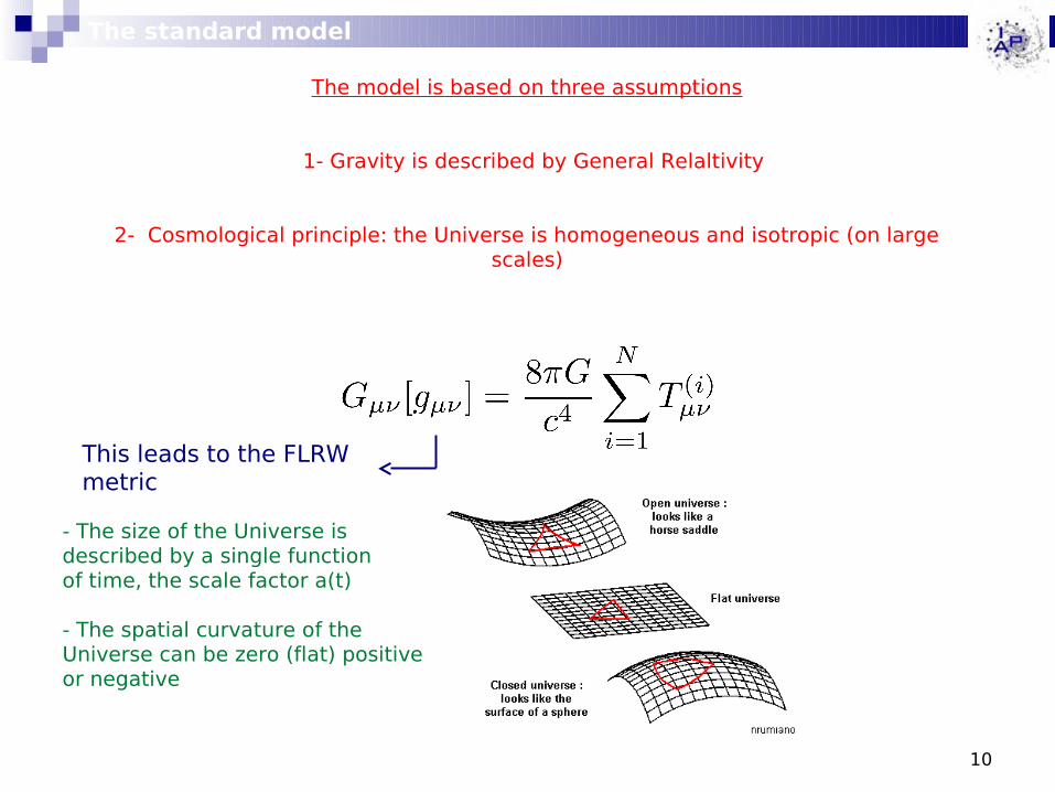
This leads to the FLRW metric
9
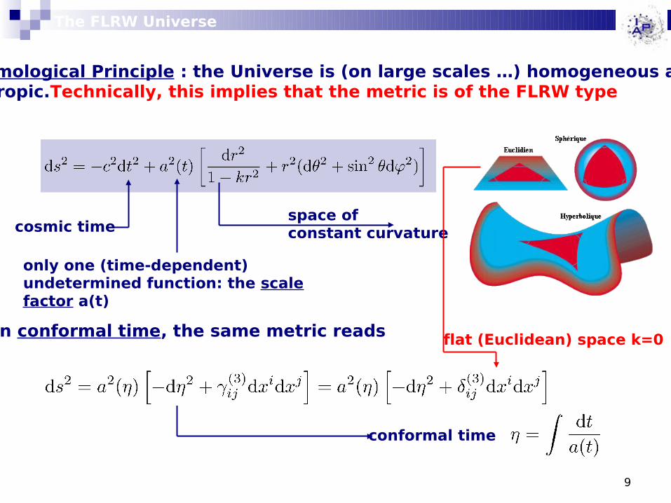
Cosmological Principle : the Universe is (on large scales …) homogeneous and isotropic.Technically, this implies that the metric is of the FLRW type
cosmic time
only one (time-dependent) undetermined function: the scale factor a(t)
space of constant curvature
In conformal time, the same metric reads
conformal time
flat (Euclidean) space k=0
The FLRW Universe
10
The standard model
The model is based on three assumptions
1- Gravity is described by General Relaltivity
2- Cosmological principle: the Universe is homogeneous and isotropic (on large scales)
- The size of the Universe is described by a single function of time, the scale factor a(t)
- The spatial curvature of the Universe can be zero (flat) positiveor negative
This leads to the FLRW metric
11
The standard model
The model is based on three assumptions
1- Gravity is described by General Relaltivity
2- Cosmological principle: the Universe is homogeneous and isotropic (on large scales)
3- Matter/energy is given by different sources to be listed in the following
This leads to the FLRW metric
- The size of the Universe is described by a single function of time, the scale factor a(t)
- The spatial curvature of the Universe can be zero (flat) positiveor negative
12
The standard model
The model is based on three assumptions
1- Gravity is described by General Relaltivity
2- Cosmological principle: the Universe is homogeneous and isotropic (on large scales)
3- Matter/energy is given by different sources to be listed in the following
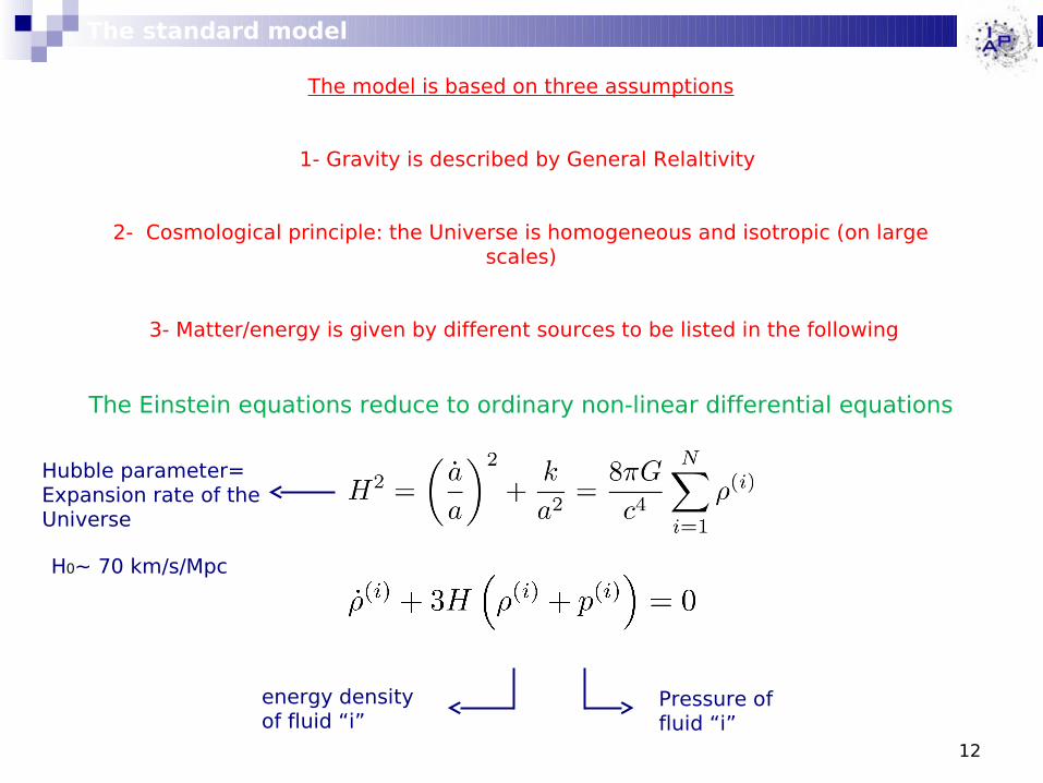
The Einstein equations reduce to ordinary non-linear differential equations
Pressure of fluid “i”
energy densityof fluid “i”
Hubble parameter=Expansion rate of the Universe
H0~ 70 km/s/Mpc
13
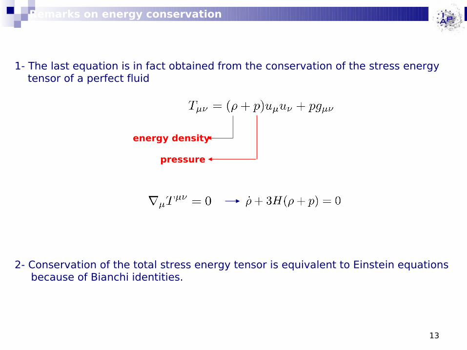
energy density
pressure
Remarks on energy conservation
1- The last equation is in fact obtained from the conservation of the stress energy tensor of a perfect fluid
2- Conservation of the total stress energy tensor is equivalent to Einstein equations because of Bianchi identities.
14
The standard model
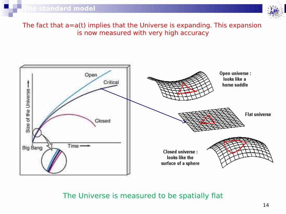
The fact that a=a(t) implies that the Universe is expanding. This expansion is now measured with very high accuracy
The Universe is measured to be spatially flat
15
time
en
erg
y d
en
si t
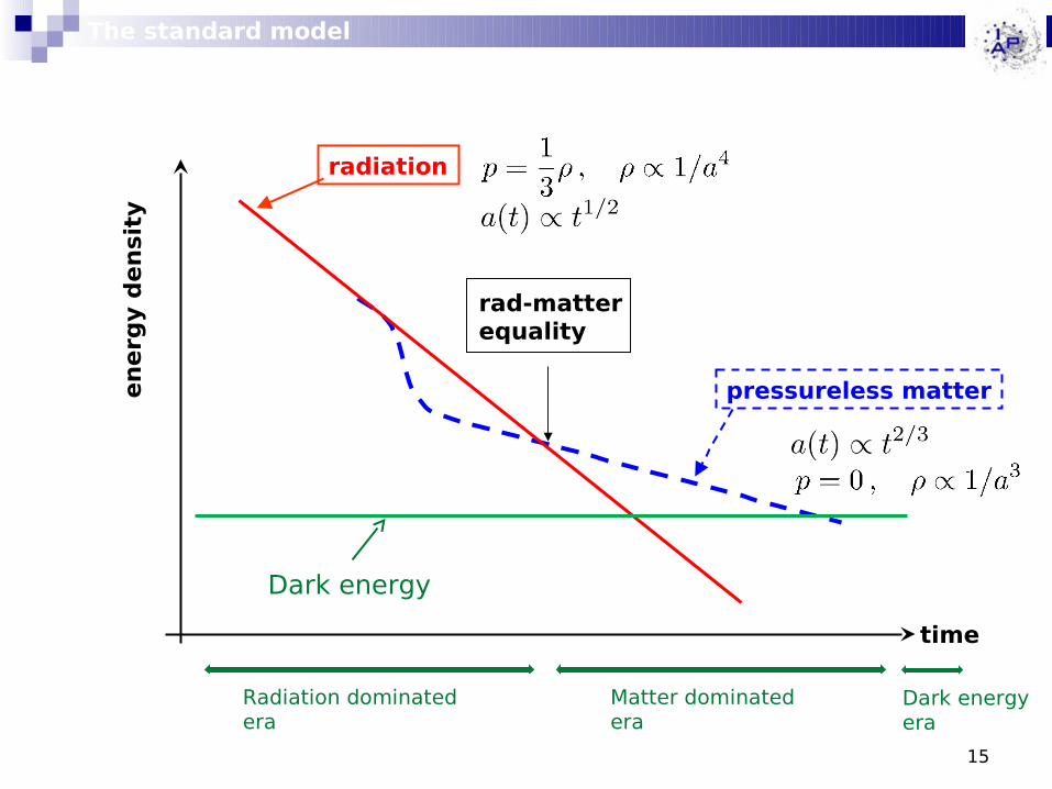
yradiation
pressureless matter
rad-matterequality
The standard model
Dark energy
Radiation dominated era
Matter dominated era
Dark energy era
16
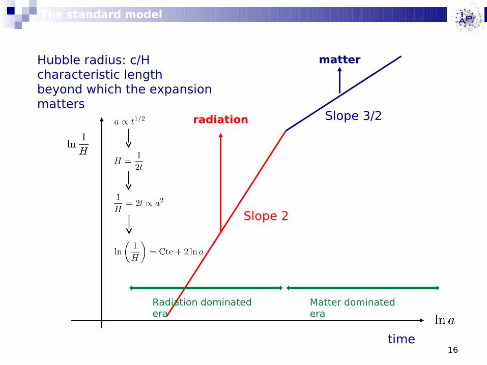
radiation
matter
Radiation dominated era
Matter dominated era
Hubble radius: c/Hcharacteristic length beyond which the expansion matters
time
The standard model
Slope 2
Slope 3/2

17
A good model!
The standard model, though it is a simple construction, can account for a
large number of observations and/or experimental tests
- Expansion (Hubble diagram)
- CMB (this school!)
- Nucleosynthesis
- etc …
18
Puzzles
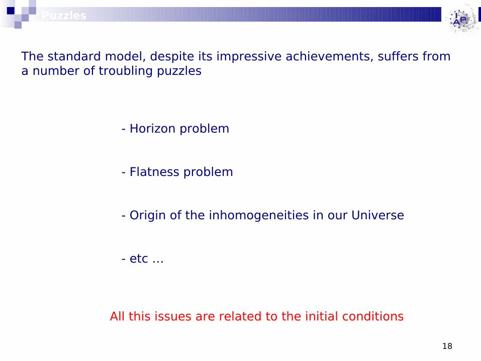
The standard model, despite its impressive achievements, suffers from a number of troubling puzzles
- Horizon problem
- Flatness problem
- Origin of the inhomogeneities in our Universe
- etc …
All this issues are related to the initial conditions
19
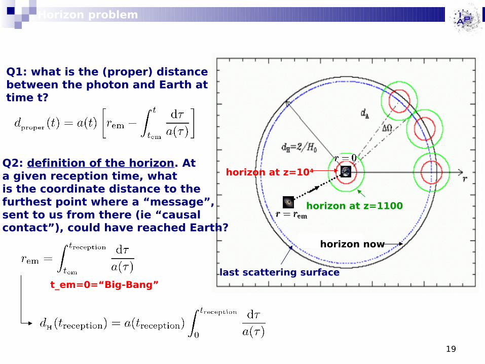
Q1: what is the (proper) distance between the photon and Earth at time t?
Q2: definition of the horizon. At a given reception time, what is the coordinate distance to the furthest point where a “message”, sent to us from there (ie “causal contact”), could have reached Earth?
horizon at z=104
horizon at z=1100
horizon now
t_em=0=“Big-Bang”
Horizon problem
last scattering surface
20
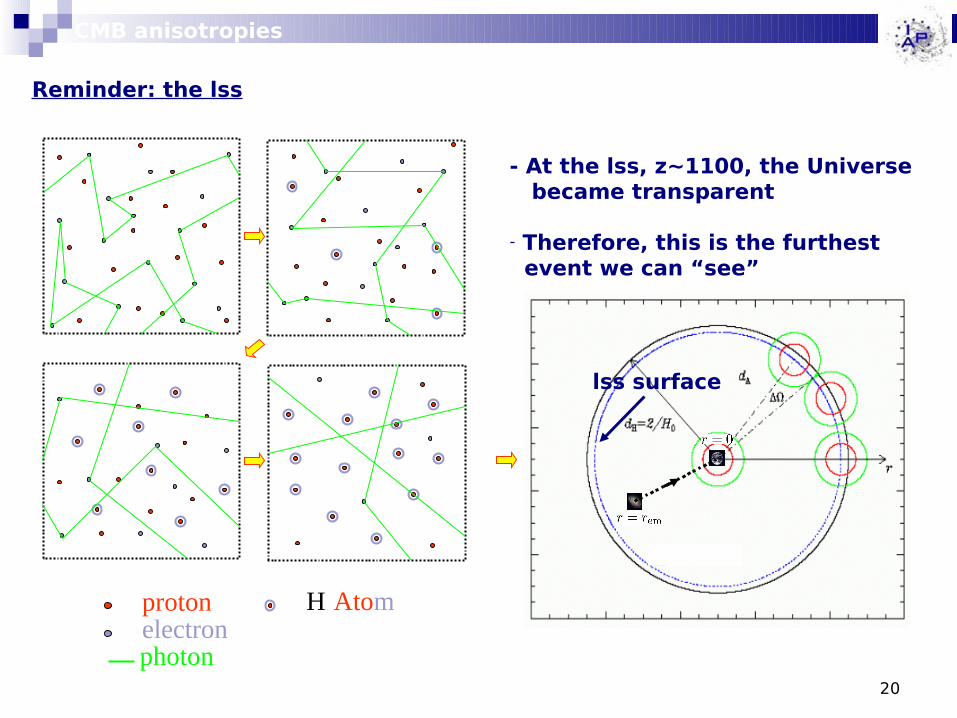
H Atomprotonelectronphoton
Reminder: the lss
CMB anisotropies
- At the lss, z~1100, the Universe became transparent
- Therefore, this is the furthest event we can “see”
Black body radiation T=2.7 K
lss surface
21
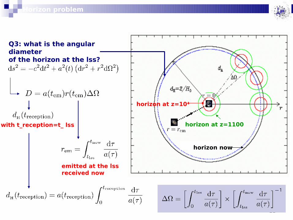
horizon at z=104
horizon at z=1100
horizon now
Q3: what is the angular diameter of the horizon at the lss?
with t_reception=t_ lss
emitted at the lss received now
Horizon problem
22
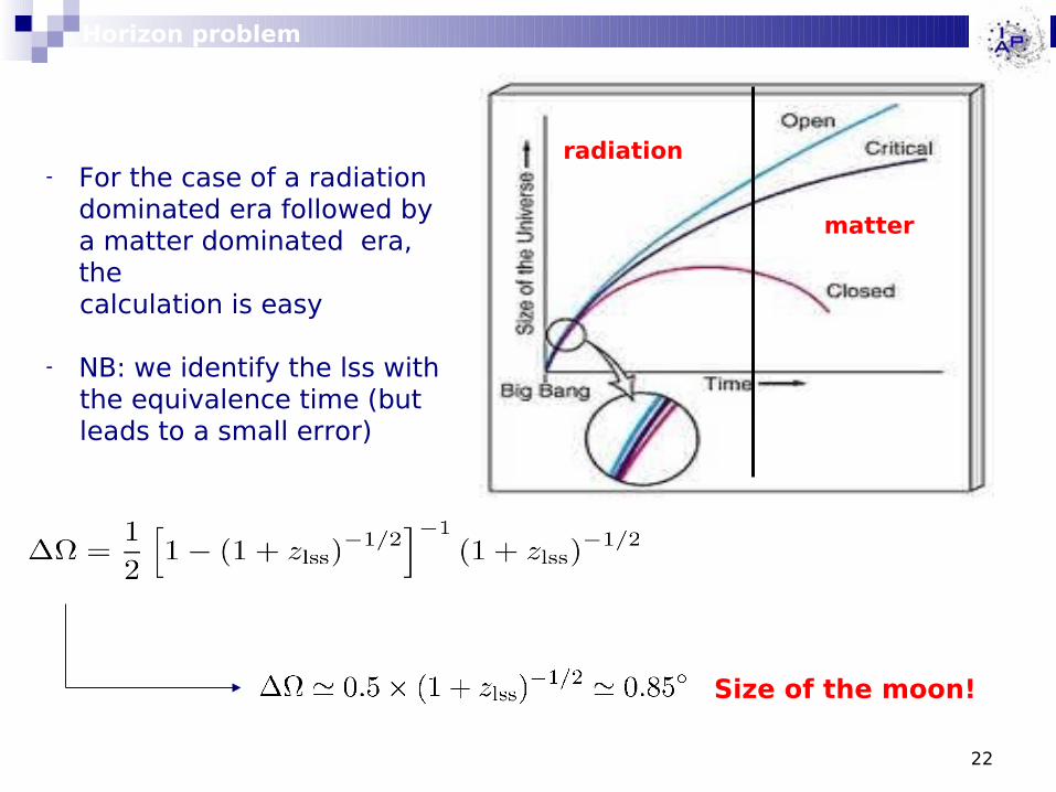
radiation
matter
Size of the moon!
- For the case of a radiation dominated era followed by a matter dominated era, the
calculation is easy
- NB: we identify the lss with the equivalence time (but leads to a small error)
Horizon problem
23
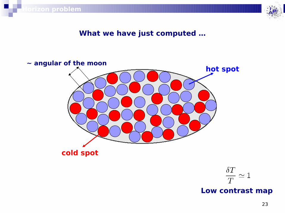
What we have just computed …
cold spot
hot spot
Low contrast map
~ angular of the moon
Horizon problem
24
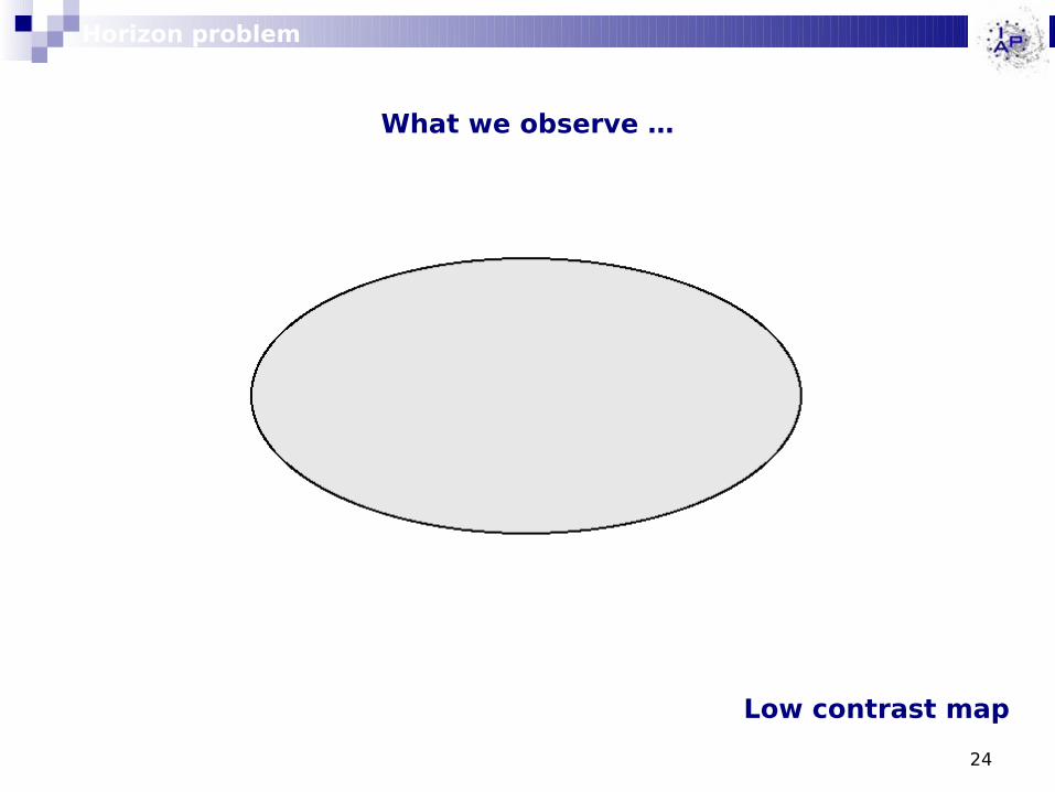
What we observe …
Low contrast map
Horizon problem
25
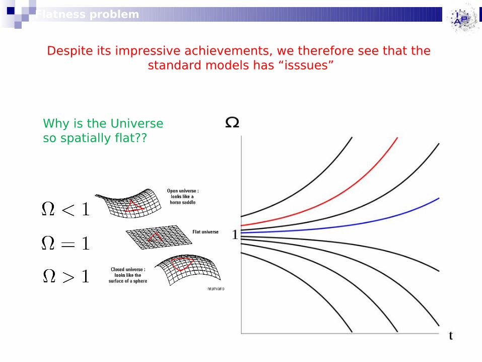
Flatness problem
Despite its impressive achievements, we therefore see that the standard models has “isssues”
Why is the Universe so spatially flat??

26
Beyond the cosmological principle
The real Universe (ie on « small » scales) is of course not homogeneous and isotropic!
27
Beyond the cosmological principle
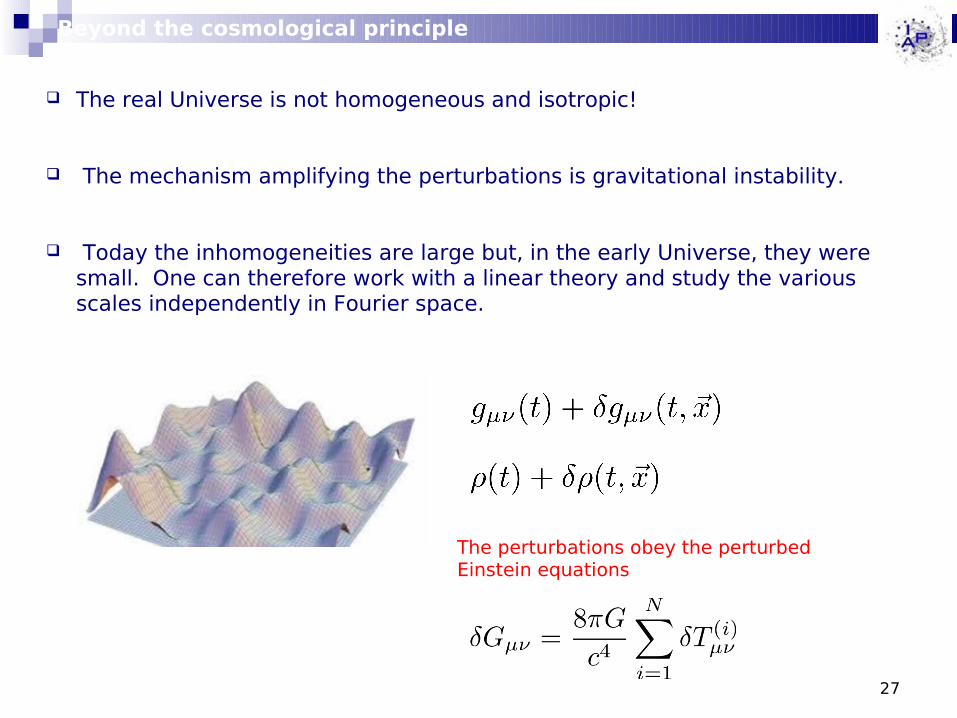
The real Universe is not homogeneous and isotropic!
The mechanism amplifying the perturbations is gravitational instability.
Today the inhomogeneities are large but, in the early Universe, they were small. One can therefore work with a linear theory and study the various scales independently in Fourier space.
The perturbations obey the perturbed Einstein equations
28
Beyond the cosmological principle
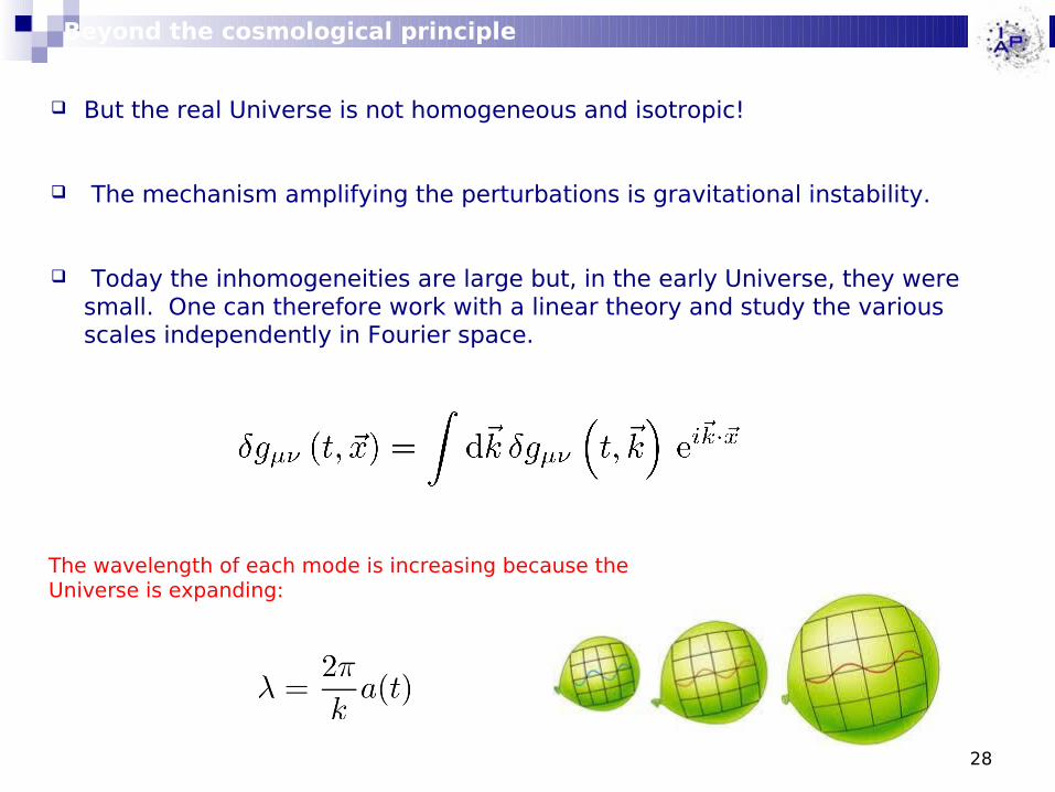
But the real Universe is not homogeneous and isotropic!
The mechanism amplifying the perturbations is gravitational instability.
Today the inhomogeneities are large but, in the early Universe, they were small. One can therefore work with a linear theory and study the various scales independently in Fourier space.
The wavelength of each mode is increasing because the Universe is expanding:
29
radiation
matter
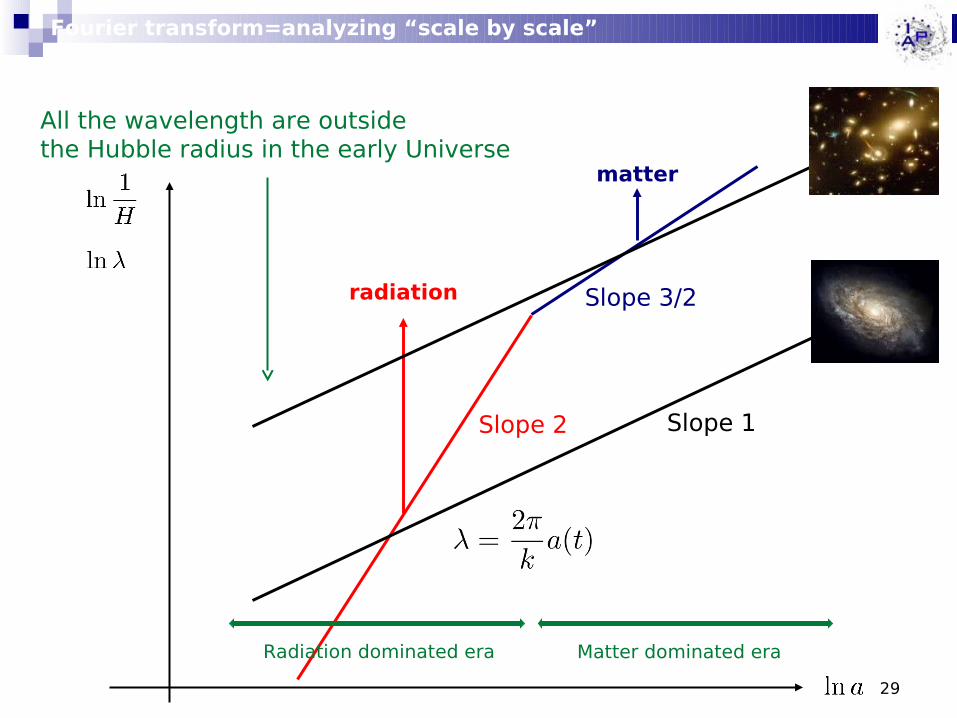
Fourier transform=analyzing “scale by scale”
Radiation dominated era Matter dominated era
All the wavelength are outside the Hubble radius in the early Universe
Slope 2
Slope 3/2
Slope 1
30
The source of the fluctuations
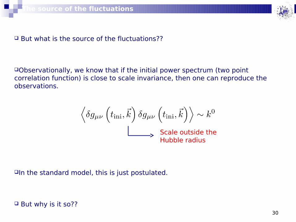
But what is the source of the fluctuations??
Observationally, we know that if the initial power spectrum (two point correlation function) is close to scale invariance, then one can reproduce the observations.
In the standard model, this is just postulated.
But why is it so??
Scale outside the Hubble radius
31
Lecture II
Lecture II: The inflationary solution
32
Puzzles of the standard model
The standard model, despite its impressive achievements, suffers from a number of troubling puzzles
- Horizon problem
- Flatness problem
- Origin of the inhomogeneities in our Universe
- etc …
All this issues are related to the initial conditions
33
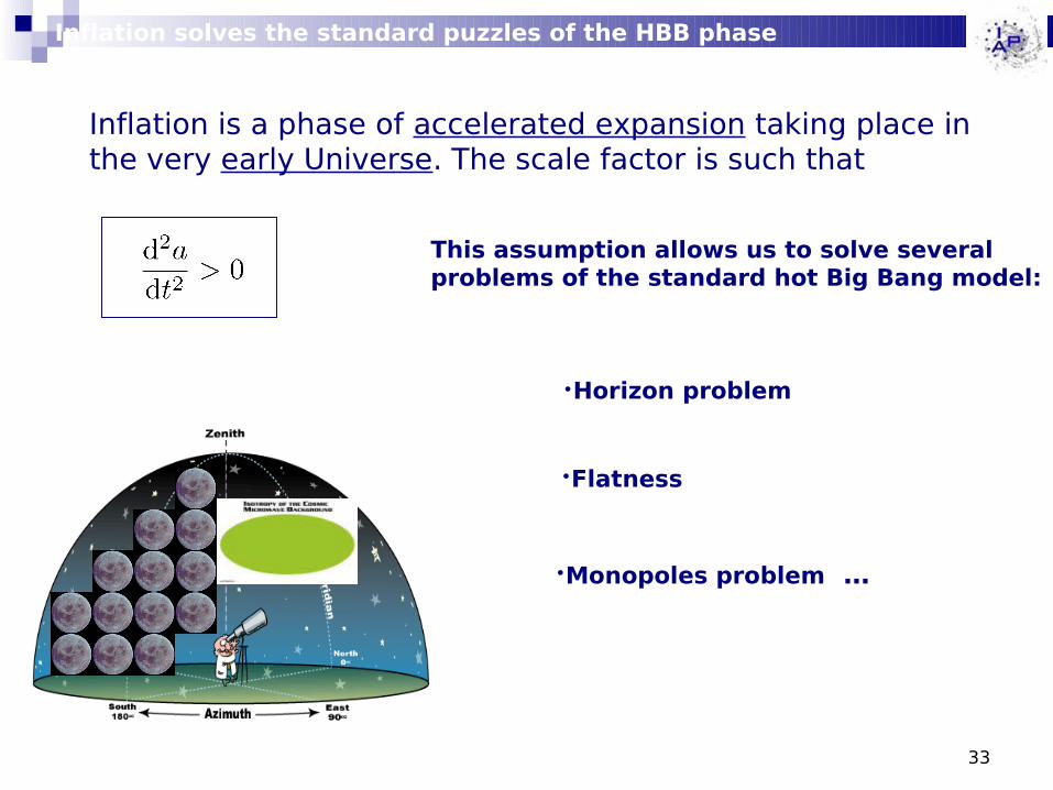
Inflation is a phase of accelerated expansion taking place in the very early Universe. The scale factor is such that
This assumption allows us to solve several problems of the standard hot Big Bang model:
•Horizon problem
•Flatness problem
•Monopoles problem …
Inflation solves the standard puzzles of the HBB phase
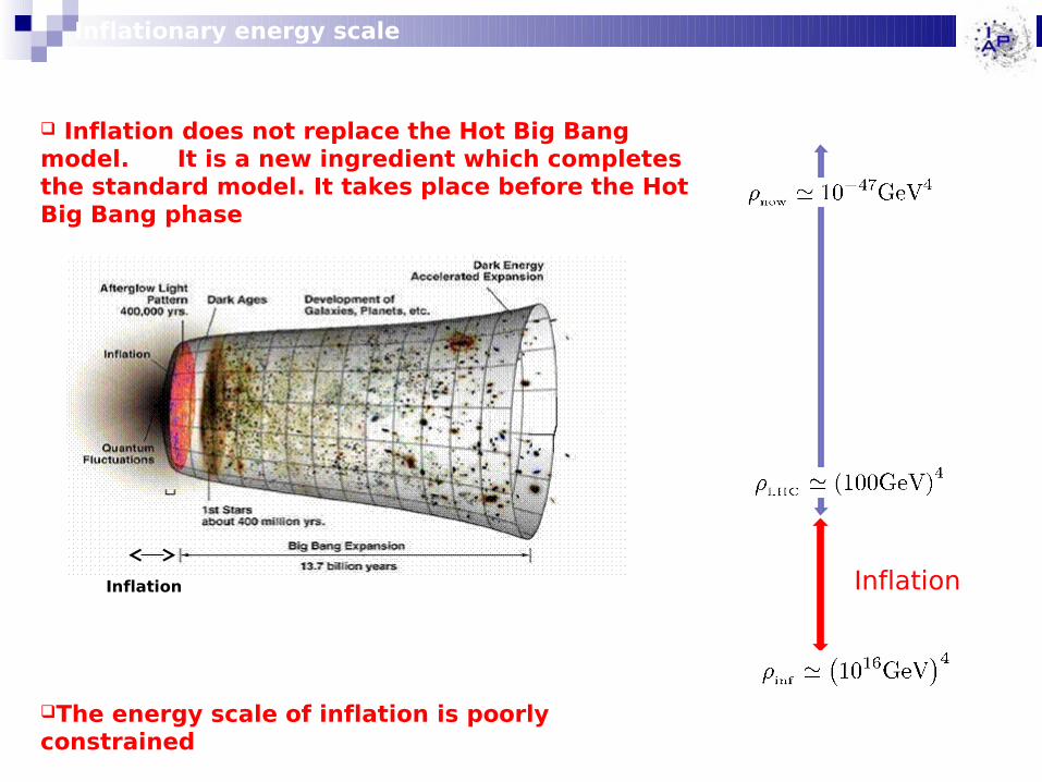
Inflationary energy scale
Inflation does not replace the Hot Big Bang model. It is a new ingredient which completes the standard model. It takes place before the Hot Big Bang phase
The energy scale of inflation is poorly constrained
InflationInflation

35
radiation unknown
matter
radiation New phase driven by an unknown fluid. Can be switched off by putting N to zero …
A simple model …
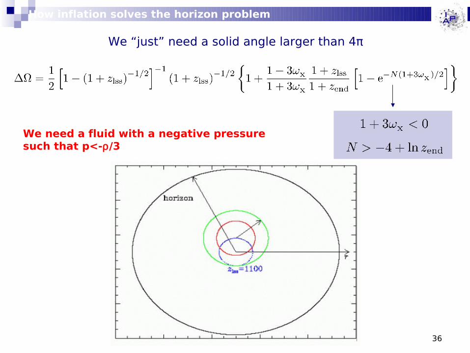
How inflation solves the horizon problem
36
We need a fluid with a negative pressure such that p<-ρ/3
How inflation solves the horizon problem
We “just” need a solid angle larger than 4π
37q
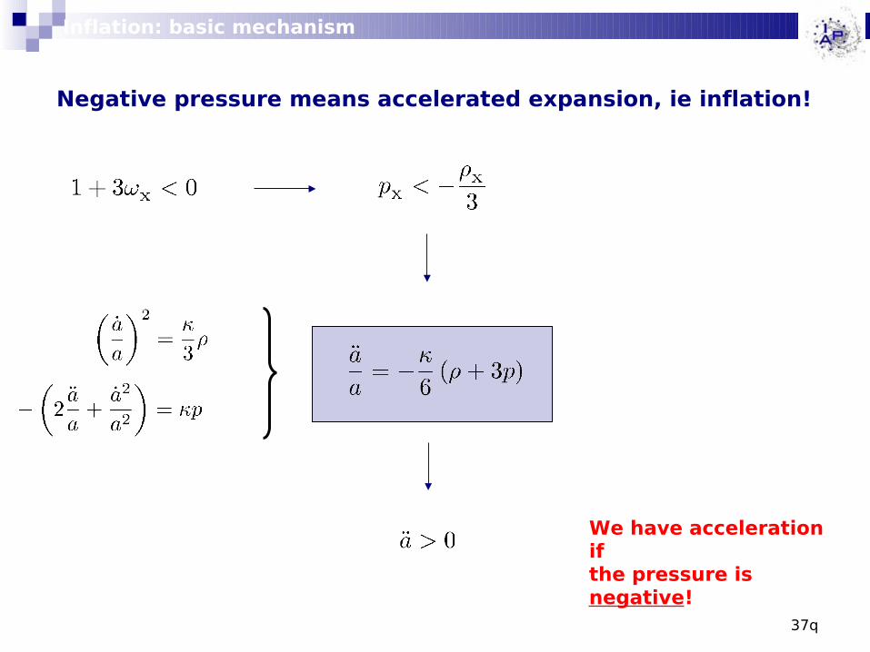
We have acceleration if the pressure is negative!
Negative pressure means accelerated expansion, ie inflation!
Inflation: basic mechanism

38
Einstein equations:
“Every form of energy weighs in General Relativity”
Inflation is possible because of GR!
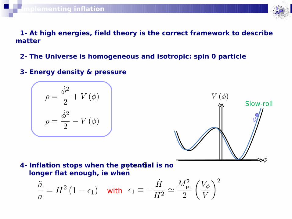
1- At high energies, field theory is the correct framework to describe matter
2- The Universe is homogeneous and isotropic: spin 0 particle
Implementing inflation
40
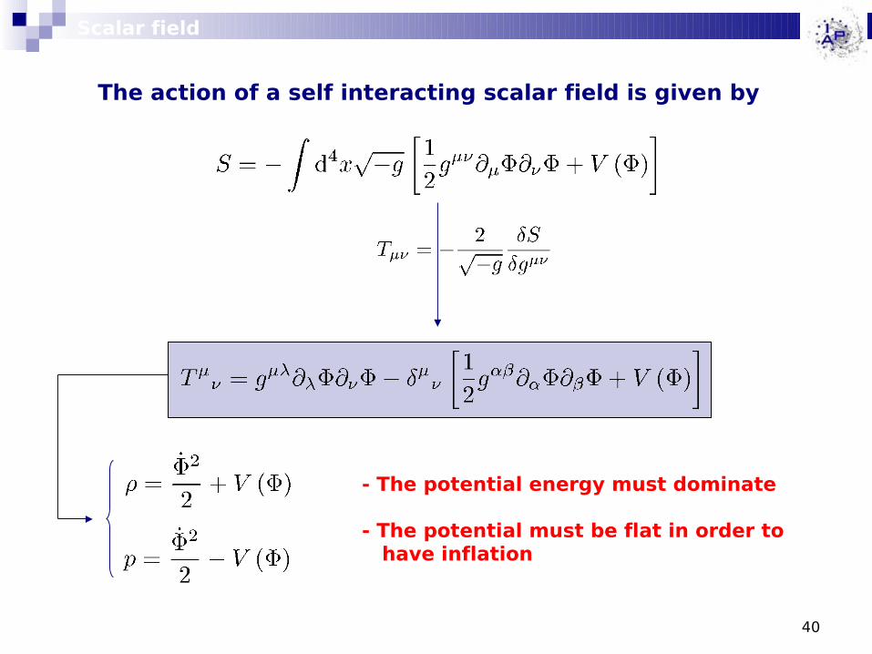
The action of a self interacting scalar field is given by
- The potential energy must dominate
- The potential must be flat in order to have inflation
Scalar field
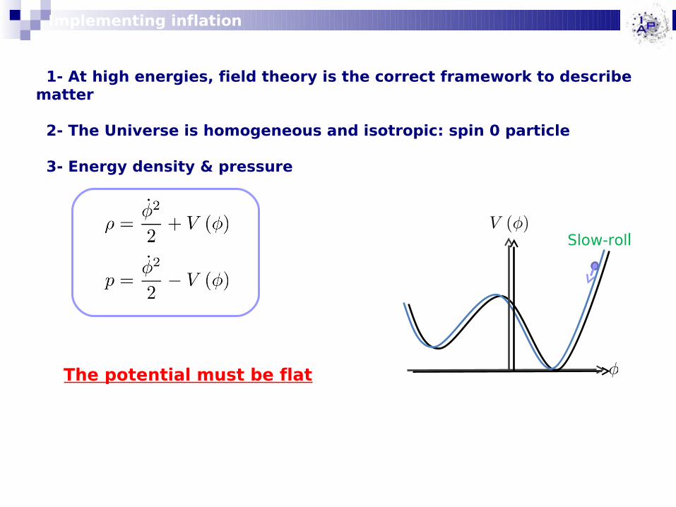
1- At high energies, field theory is the correct framework to describe matter
2- The Universe is homogeneous and isotropic: spin 0 particle
3- Energy density & pressure
Implementing inflation
Slow-roll
The potential must be flat
1- At high energies, field theory is the correct framework to describe matter
2- The Universe is homogeneous and isotropic: spin 0 particle
3- Energy density & pressure
4- Inflation stops when the potential is no longer flat enough, ie when
Implementing inflation
Slow-roll
with
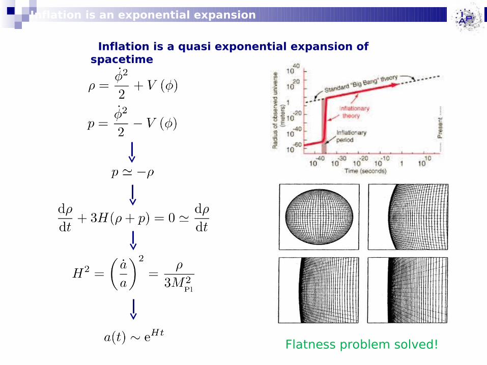
Inflation is a quasi exponential expansion of spacetime
Inflation is an exponential expansion
Flatness problem solved!

Inflation is a quasi exponential expansion of spacetime
Inflation is an exponential expansion
The Hubble radius 1/H is almost constantduring inflation

45
radiation matterInflation: the Hubble parameter is almost constant (exact for de Sitter).
Fourier transform=analyzing “scale by scale”
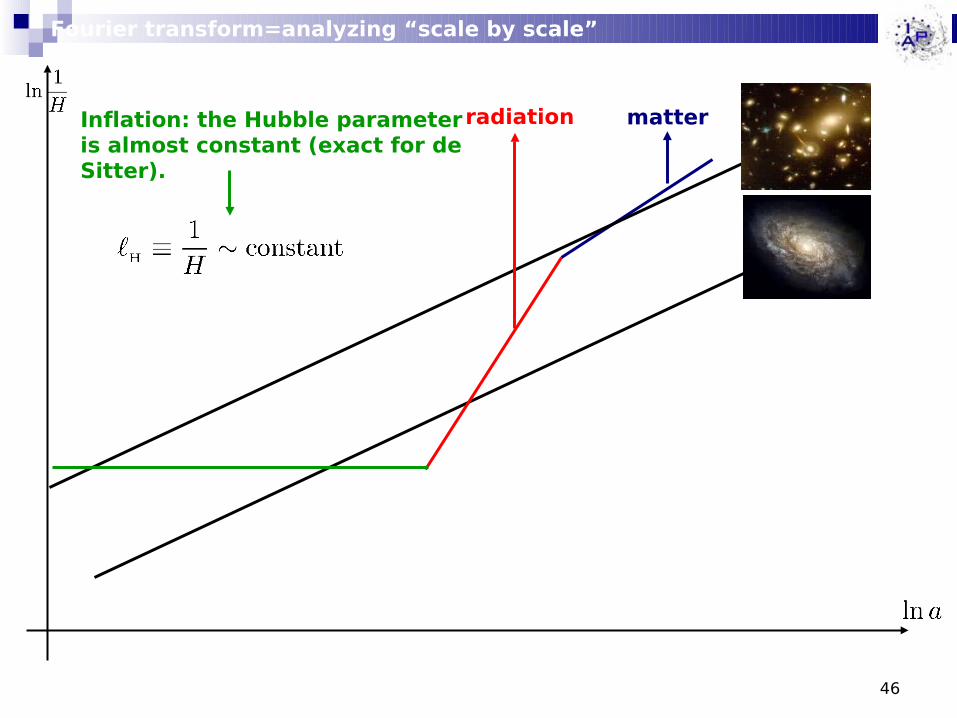
46
radiation matterInflation: the Hubble parameter is almost constant (exact for de Sitter).
Fourier transform=analyzing “scale by scale”
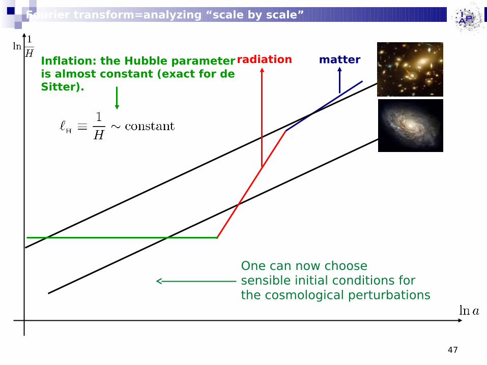
47
radiation matterInflation: the Hubble parameter is almost constant (exact for de Sitter).
Fourier transform=analyzing “scale by scale”
One can now choose sensible initial conditions for the cosmological perturbations
48
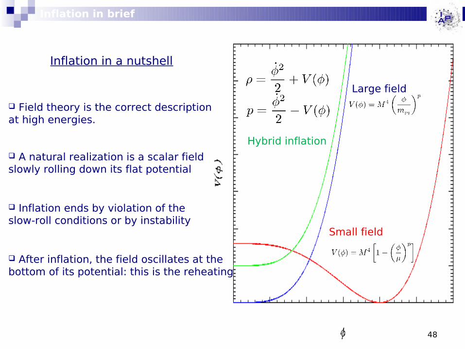
Field theory is the correct description at high energies.
A natural realization is a scalar field slowly rolling down its flat potential
Inflation ends by violation of the slow-roll conditions or by instability
After inflation, the field oscillates at the bottom of its potential: this is the reheating
Inflation in brief
Inflation in a nutshell
Large field
Small field
Hybrid inflation
49
End of Inflation (I)
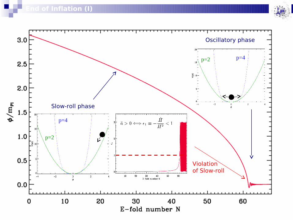
Slow-roll phase
Oscillatory phase
p=2
p=4
p=2 p=4
Violation of Slow-roll
50
End of Inflation (II)
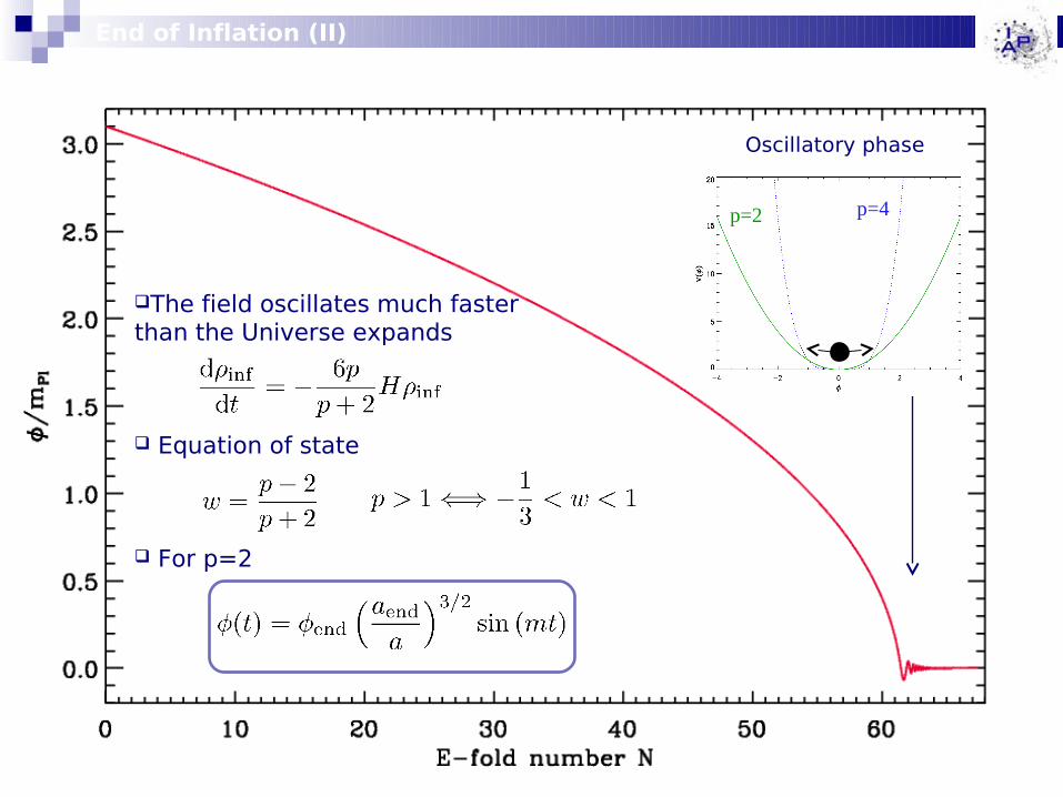
Oscillatory phase
p=2 p=4
The field oscillates much faster than the Universe expands
Equation of state
For p=2
51
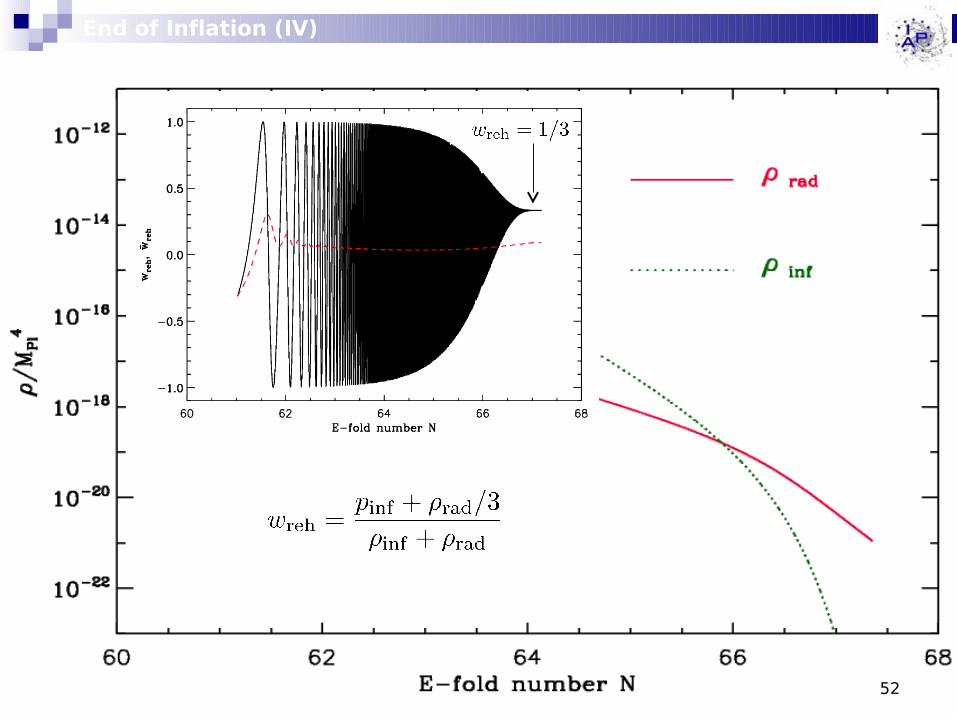
End of Inflation (III)
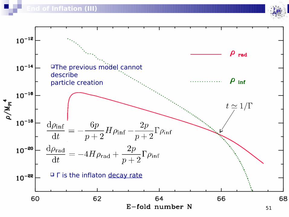
The previous model cannot describe particle creation
Γ is the inflaton decay rate
52
End of Inflation (IV)
53
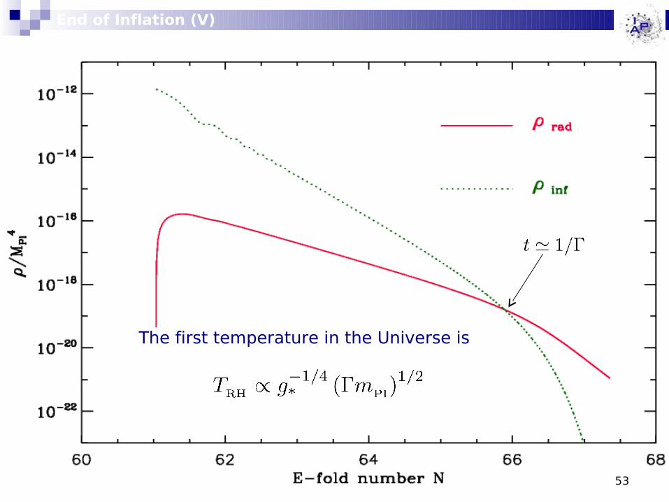
End of Inflation (V)
The first temperature in the Universe is
54
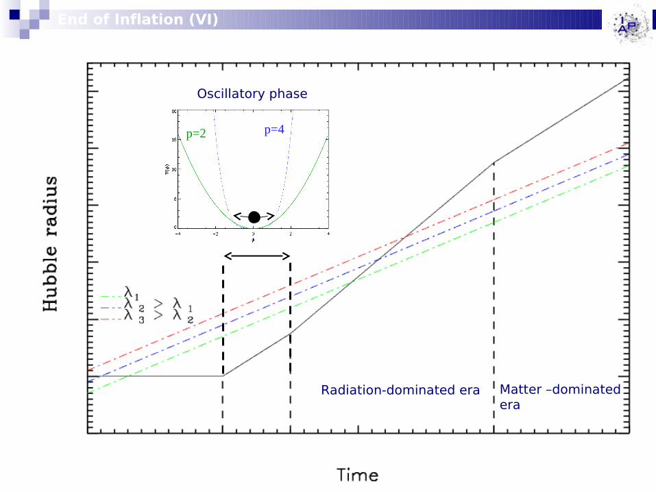
End of Inflation (VI)
Oscillatory phase
Radiation-dominated era Matter –dominated era
p=2 p=4
55
Reheating era (II)
So far we do not know so much on the reheating temperature, ie (can be (improved – the upper bound- if gravitinos production is taken into account)
ρend>ρreh>ρBBN
The previous description is a naive description of the infaton/rest of the world coupling. It can be much more complicated.
Theory of preheating, thermalization etc …
How does the reheating affect the inflationary predictions?
It modifies the relation between the physical scales now and the number of e-folds at which perturbations left the Hubble radius
Can the oscillations of the inflaton affect the behaviour of the perturbations?
Consequences of reheating
Implementing Inflation
The common way to realize inflation is to assume that there is a scalar field (or several scalar fields) dominating in the early Universe
Implementing Inflation (II)
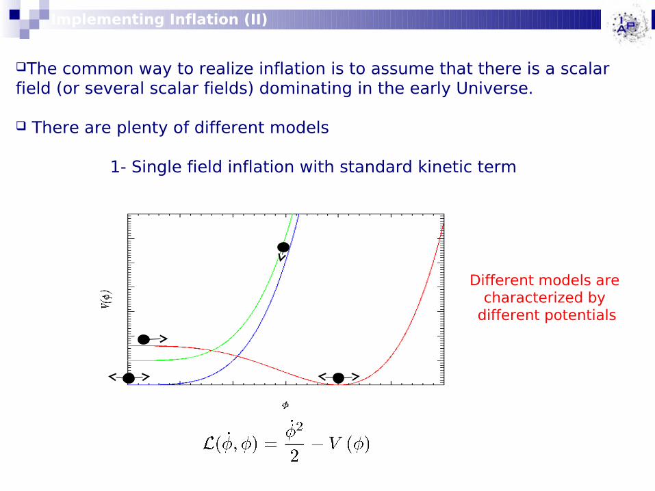
The common way to realize inflation is to assume that there is a scalar field (or several scalar fields) dominating in the early Universe.
There are plenty of different models
1- Single field inflation with standard kinetic term
Different models are characterized by
different potentials
Implementing Inflation (III)
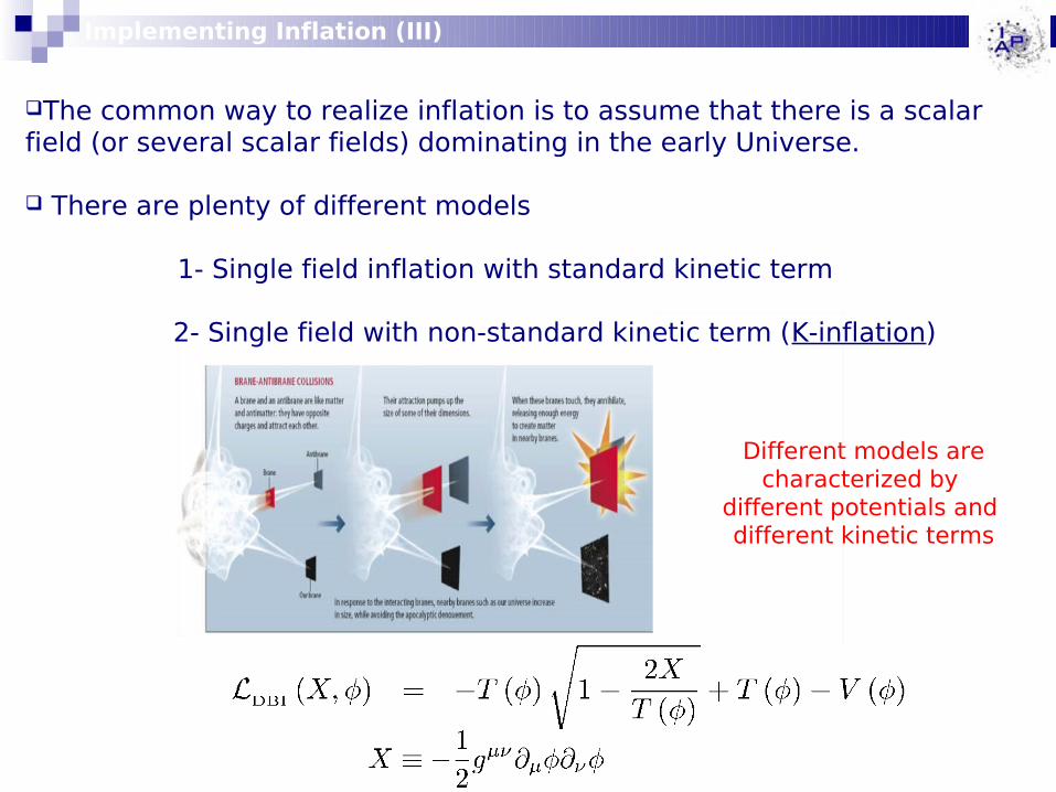
The common way to realize inflation is to assume that there is a scalar field (or several scalar fields) dominating in the early Universe.
There are plenty of different models
1- Single field inflation with standard kinetic term
2- Single field with non-standard kinetic term (K-inflation)
Different models are characterized by
different potentials and different kinetic terms
Implementing Inflation (IV)
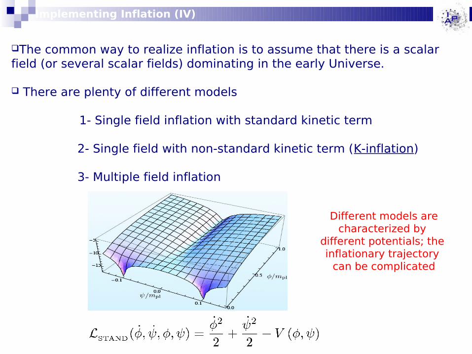
The common way to realize inflation is to assume that there is a scalar field (or several scalar fields) dominating in the early Universe.
There are plenty of different models
1- Single field inflation with standard kinetic term
2- Single field with non-standard kinetic term (K-inflation)
3- Multiple field inflation
Different models are characterized by
different potentials; the inflationary trajectory
can be complicated
60
Lecture III
Lecture III: inflationary perturbations of quantum-mechanical origin
61
Puzzles of the standard model
The standard model, despite its impressive achievements, suffers from a number of troubling puzzles
- Horizon problem
- Flatness problem
- Origin of the inhomogeneities in our Universe
- etc …
All this issues are related to the initial conditions
62
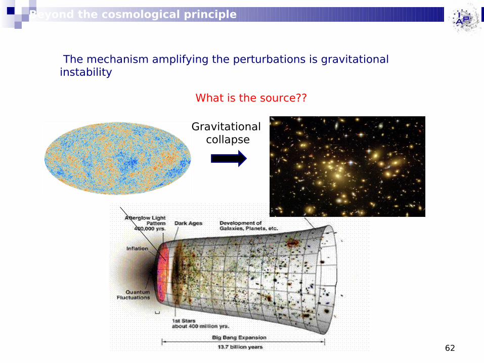
Beyond the cosmological principle
The mechanism amplifying the perturbations is gravitational instability
What is the source??
Gravitational collapse
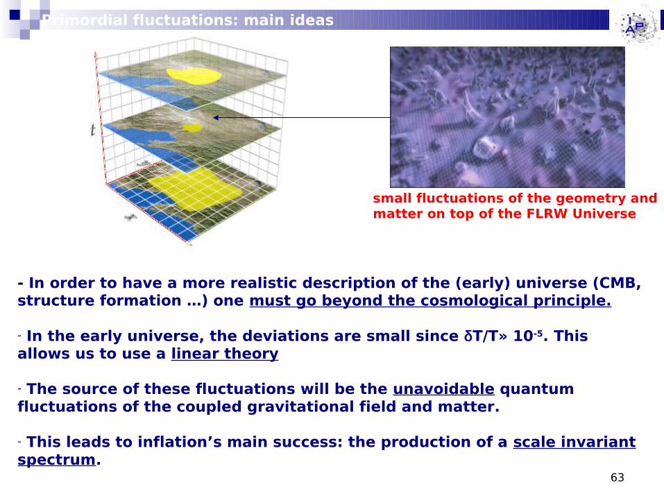
- In order to have a more realistic description of the (early) universe (CMB, structure formation …) one must go beyond the cosmological principle.
- In the early universe, the deviations are small since δT/T» 10-5. This allows us to use a linear theory
- The source of these fluctuations will be the unavoidable quantum fluctuations of the coupled gravitational field and matter.
- This leads to inflation’s main success: the production of a scale invariant spectrum.
small fluctuations of the geometry and matter on top of the FLRW Universe
Primordial fluctuations: main ideas
63
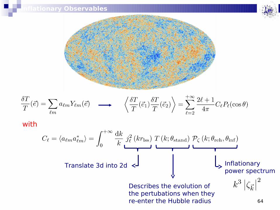
64
Inflationary Observables
with
Translate 3d into 2d
Describes the evolution of the pertubations when they re-enter the Hubble radius
Inflationarypower spectrum
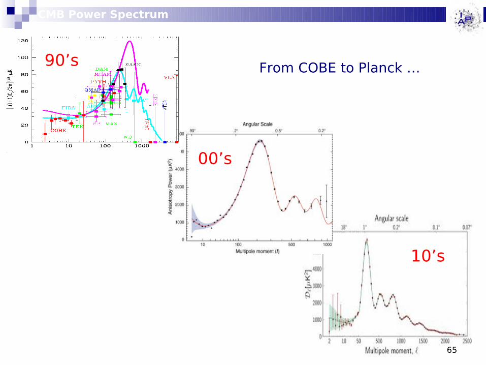
CMB Power Spectrum
65
90’s
00’s
10’s
From COBE to Planck …
inflation radiation matter
,
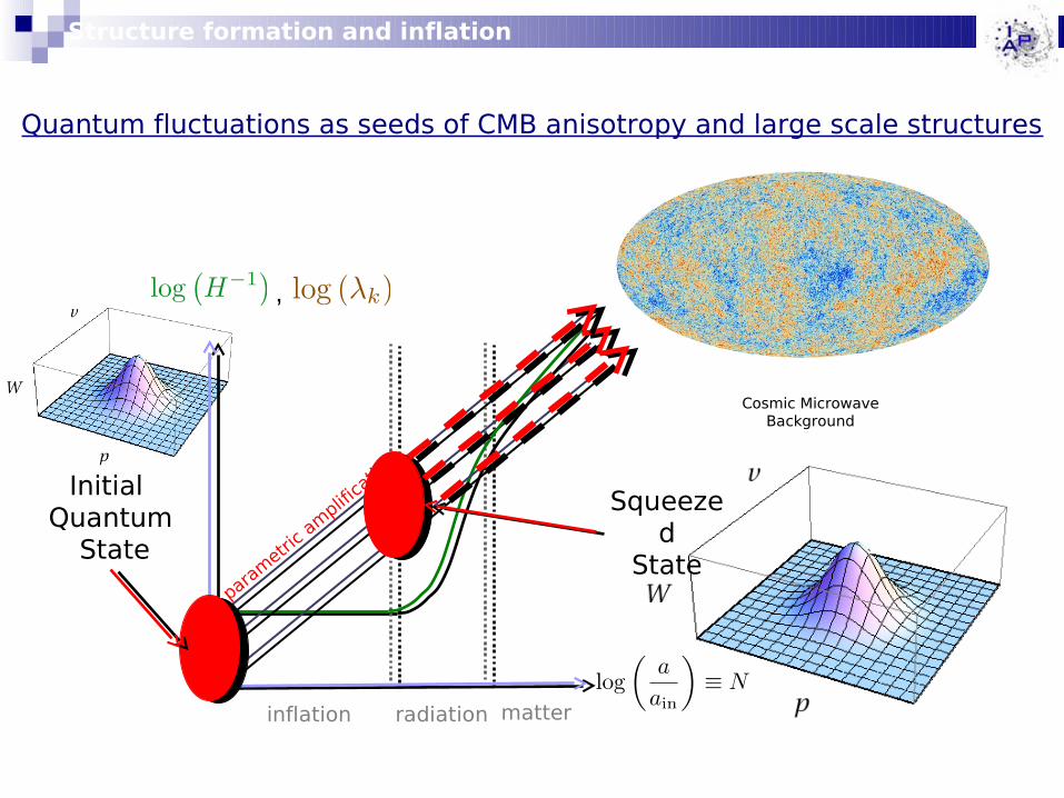
param
etric
am
plifica
tion
Initial Quantum
State
Cosmic Microwave Background
Squeezed
State
Quantum fluctuations as seeds of CMB anisotropy and large scale structures
Structure formation and inflation
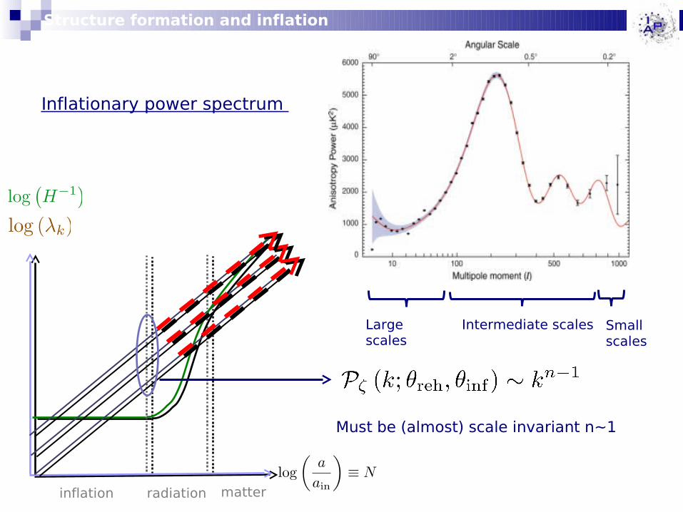
inflation radiation matter
Structure formation and inflation
Large scales
Intermediate scales Small scales
Must be (almost) scale invariant n~1
Inflationary power spectrum
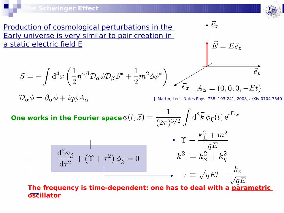
The Schwinger Effect
Production of cosmological perturbations in the Early universe is very similar to pair creation in a static electric field E
The frequency is time-dependent: one has to deal with a parametric oscillator
One works in the Fourier space
J. Martin, Lect. Notes Phys. 738: 193-241, 2008, arXiv:0704.3540

69
Schwinger effect Inflationary cosmological perturbations
- Scalar field
- Classical electric field
- Amplitude of the effect controlled by E
- Perturbed metric
- Background gravitational field: scale factor
- Amplitude controlled by the Hubble parameter H
Inflationary fluctuations
The inflationary mechanism is a conservative one: similar to the Schwinger effect in QFT
70
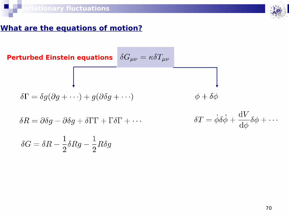
What are the equations of motion?
Perturbed Einstein equations
Inflationary fluctuations
71
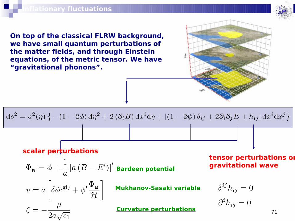
On top of the classical FLRW background, we have small quantum perturbations of the matter fields, and through Einstein equations, of the metric tensor. We have “gravitational phonons”.
scalar perturbationstensor perturbations or gravitational waveBardeen potential
Mukhanov-Sasaki variable
Inflationary fluctuations
Curvature perturbations
72
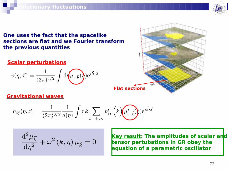
One uses the fact that the spacelike sections are flat and we Fourier transform the previous quantities
Scalar perturbations
Gravitational waves
Key result: The amplitudes of scalar and tensor pertubations in GR obey the equation of a parametric oscillator
Flat sections
Inflationary fluctuations
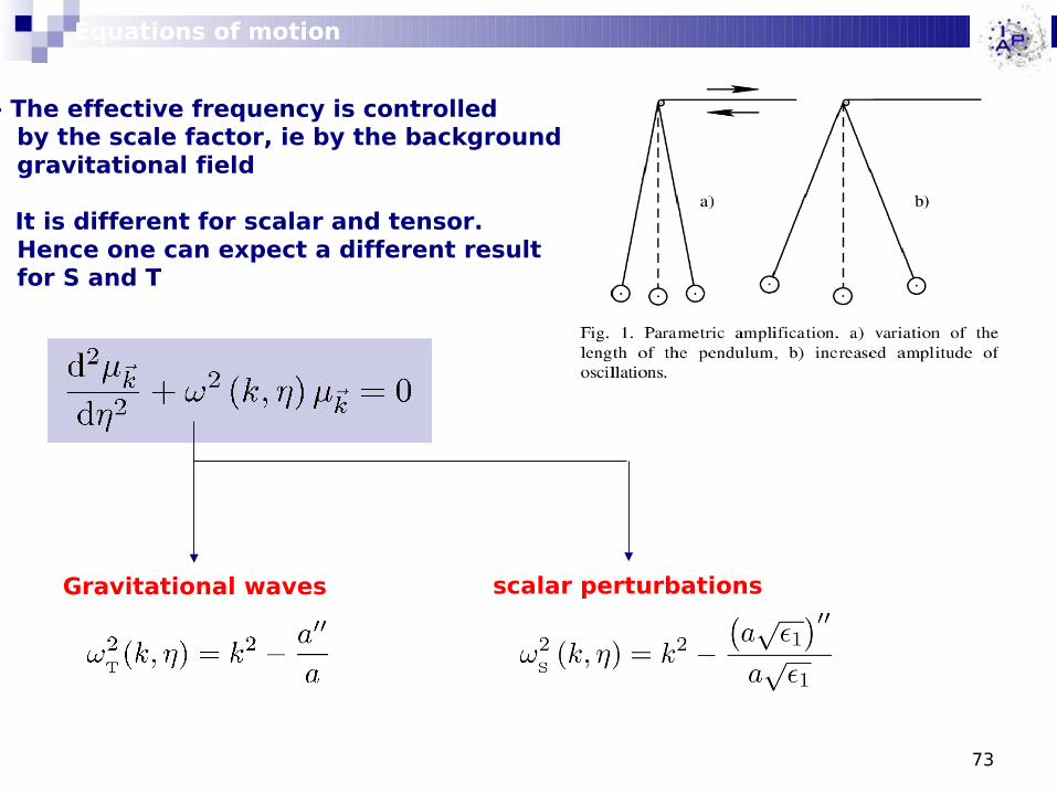
73
Equations of motion
Gravitational waves
- The effective frequency is controlled by the scale factor, ie by the background gravitational field
- It is different for scalar and tensor. Hence one can expect a different result for S and T
scalar perturbations
inflation radiation matter
param
etric
amplifi
catio
n
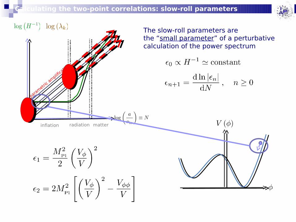
The slow-roll parameters are the “small parameter” of a perturbative calculation of the power spectrum
Calculating the two-point correlations: slow-roll parameters
75
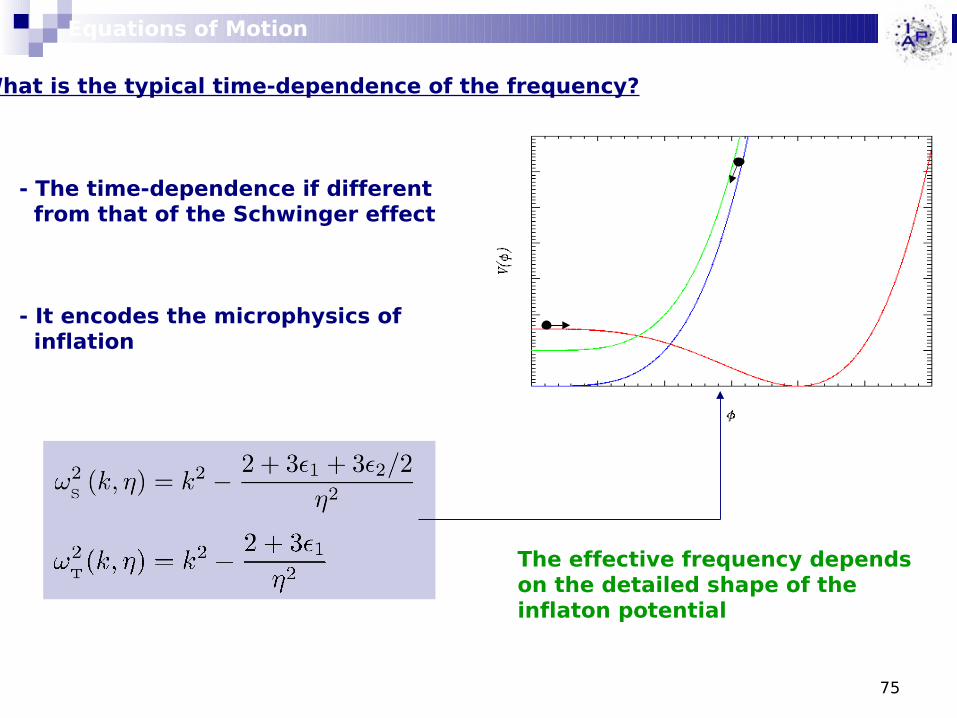
What is the typical time-dependence of the frequency?
- The time-dependence if different from that of the Schwinger effect
- It encodes the microphysics of inflation
The effective frequency depends on the detailed shape of the inflaton potential
Equations of Motion
76
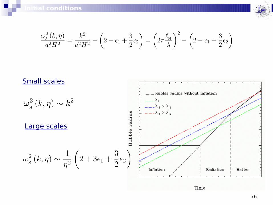
Initial conditions
Small scales
Large scales

77
Which initial conditions?
Key assumption: one choose the adiabatic vacuum initially
Initial conditions
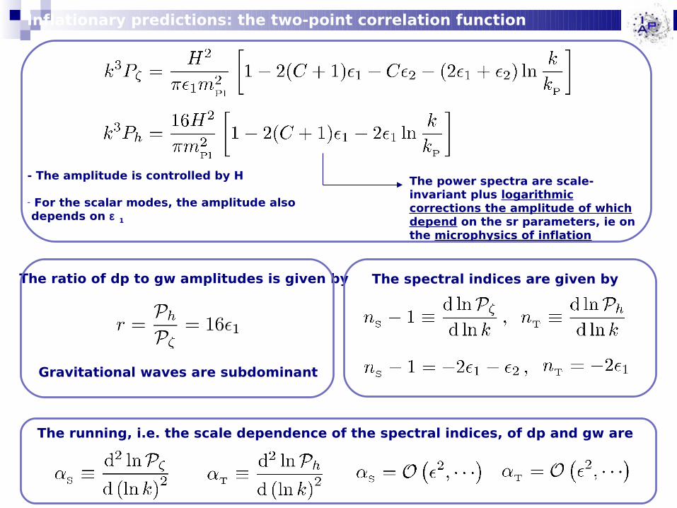
The ratio of dp to gw amplitudes is given by
Gravitational waves are subdominant
The spectral indices are given by
The running, i.e. the scale dependence of the spectral indices, of dp and gw are
Inflationary predictions: the two-point correlation function
- The amplitude is controlled by H
- For the scalar modes, the amplitude also depends on ε 1
The power spectra are scale-invariant plus logarithmic corrections the amplitude of which depend on the sr parameters, ie on the microphysics of inflation
79
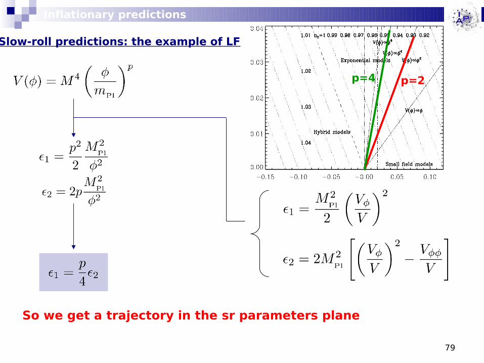
Slow-roll predictions: the example of LF
So we get a trajectory in the sr parameters plane
p=2p=4
Inflationary predictions
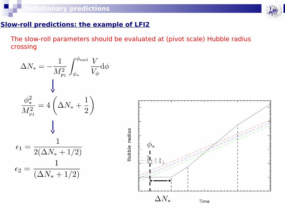
Slow-roll predictions: the example of LFI2
The slow-roll parameters should be evaluated at (pivot scale) Hubble radius crossing
Inflationary predictions
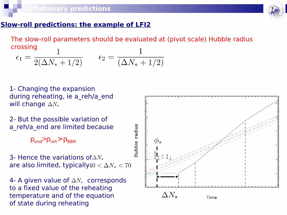
Slow-roll predictions: the example of LFI2
The slow-roll parameters should be evaluated at (pivot scale) Hubble radius crossing
Inflationary predictions
1- Changing the expansion during reheating, ie a_reh/a_endwill change
2- But the possible variation of a_reh/a_end are limited because
3- Hence the variations of are also limited, typically
4- A given value of corresponds to a fixed value of the reheating temperature and of the equation of state during reheating
ρend>ρreh>ρBBN
82
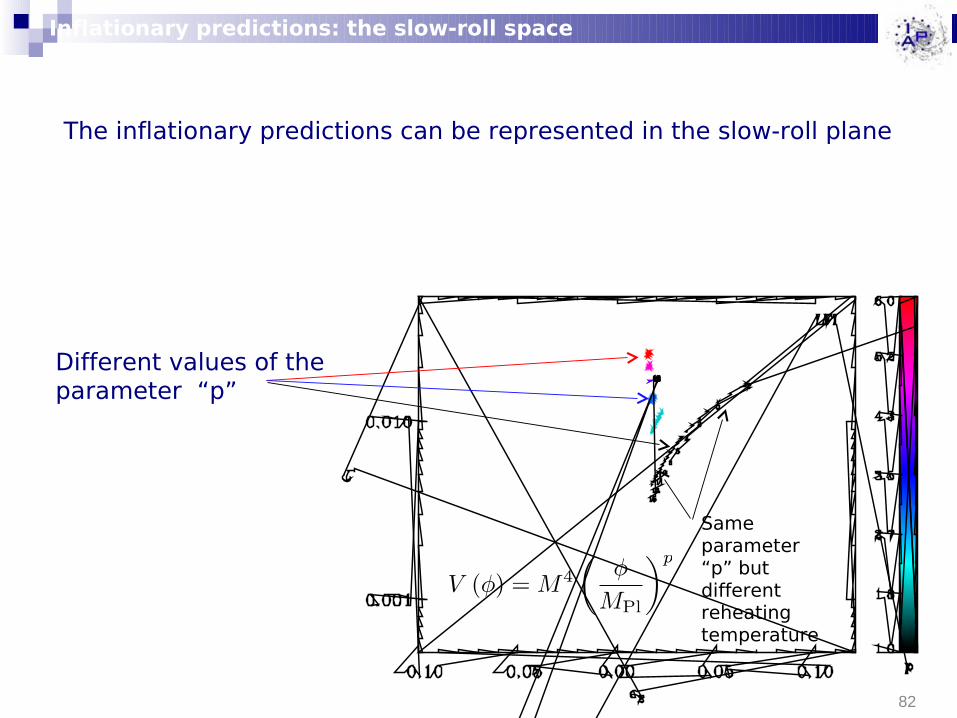
The inflationary predictions can be represented in the slow-roll plane
Different values of the parameter “p”
Inflationary predictions: the slow-roll space
Same parameter “p” but different reheating temperature
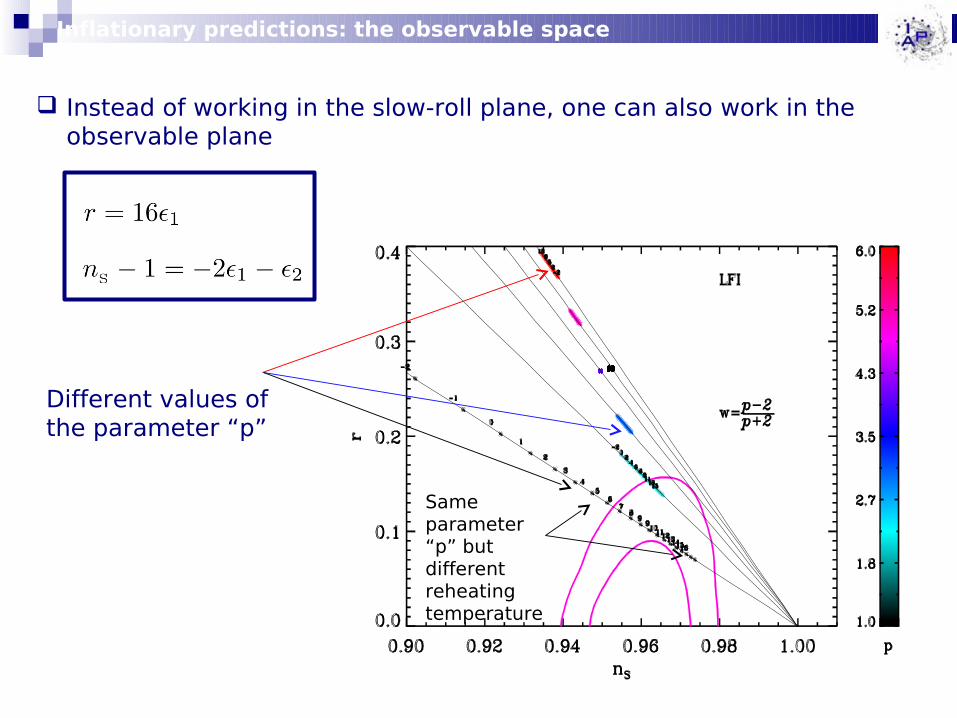
Inflationary predictions: the observable space
Instead of working in the slow-roll plane, one can also work in the observable plane
Different values of the parameter “p”
Same parameter “p” but different reheating temperature
84
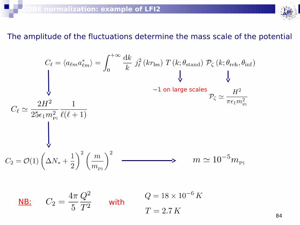
COBE normalization: example of LFI2
The amplitude of the fluctuations determine the mass scale of the potential
~1 on large scales
NB: with

85
Lecture IV
Lecture IV: inflation after Planck
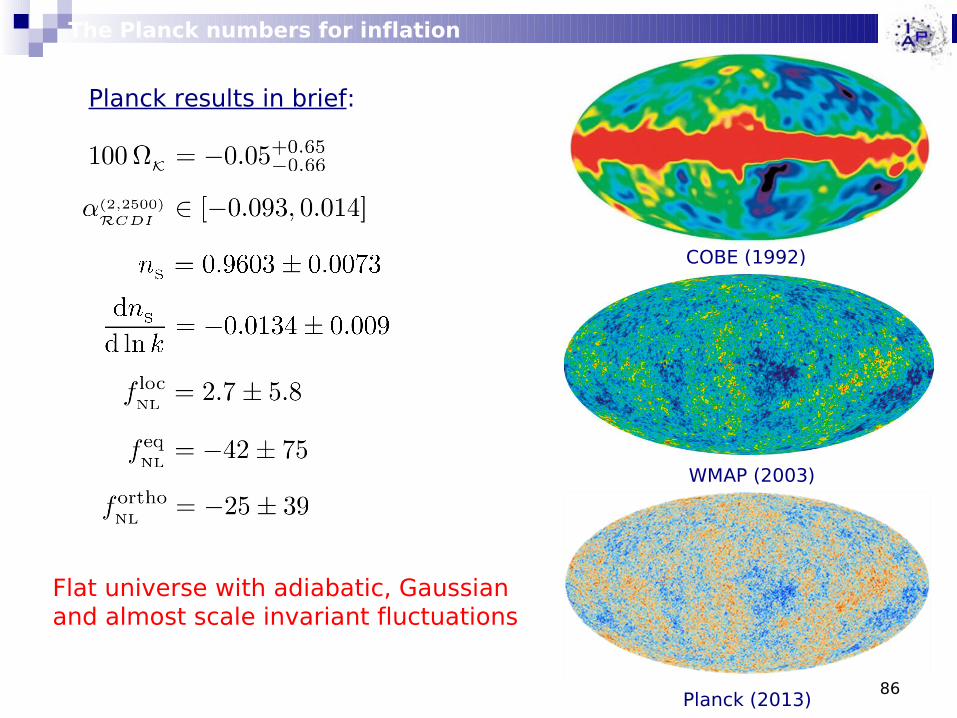
The Planck numbers for inflation
86
COBE (1992)
WMAP (2003)
Planck (2013)
Planck results in brief:
Flat universe with adiabatic, Gaussian and almost scale invariant fluctuations
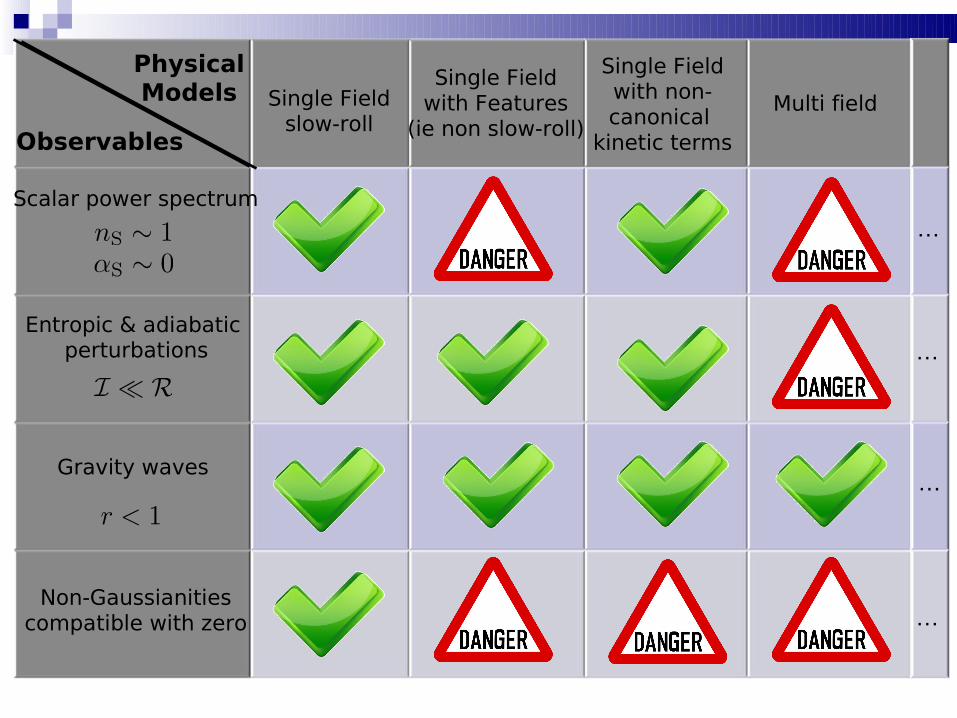
Entropic & adiabatic perturbations
Scalar power spectrum
Gravity waves
Non-Gaussianitiescompatible with zero
Single Fieldslow-roll
Single Fieldwith non-canonical
kinetic terms
Multi fieldSingle Field
with Features(ie non slow-roll)
PhysicalModels
Observables
…
…
…
…
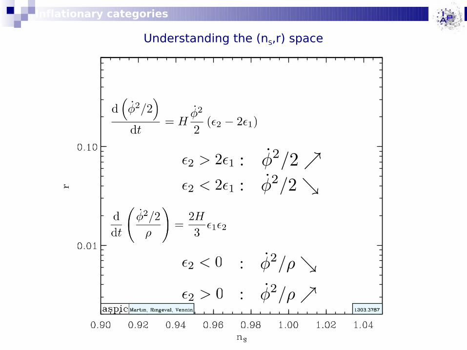
Understanding the (nS,r) space
Inflationary categories

Understanding the (nS,r) space
Inflationary categories
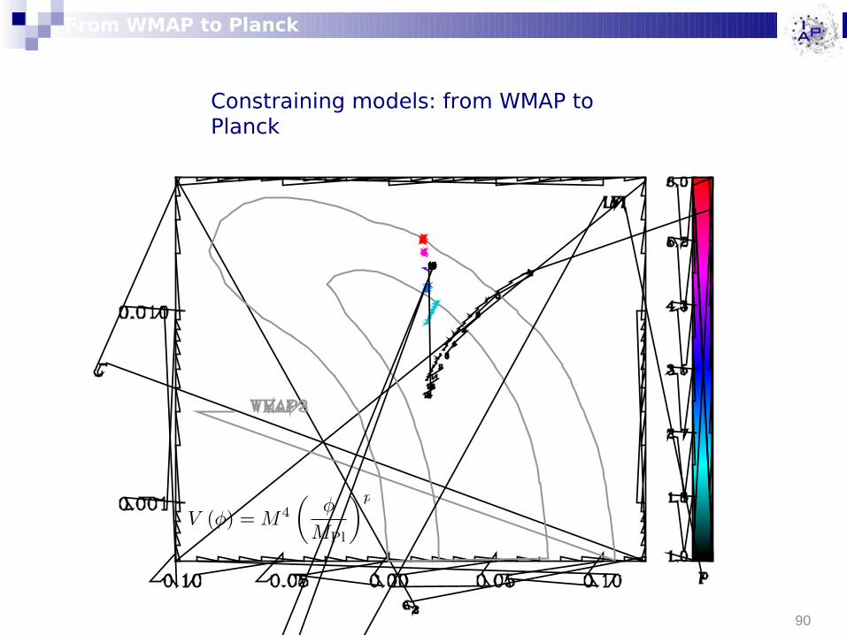
Constraining models: from WMAP to Planck
90
From WMAP to Planck
91
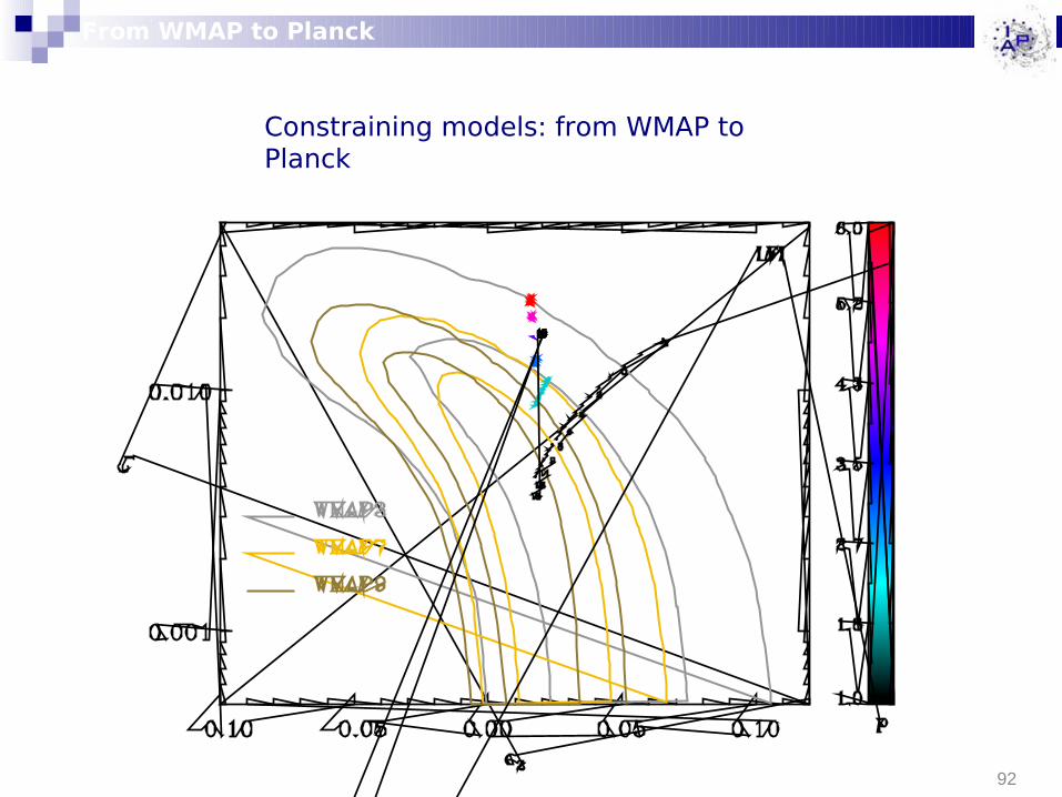
Constraining models: from WMAP to Planck
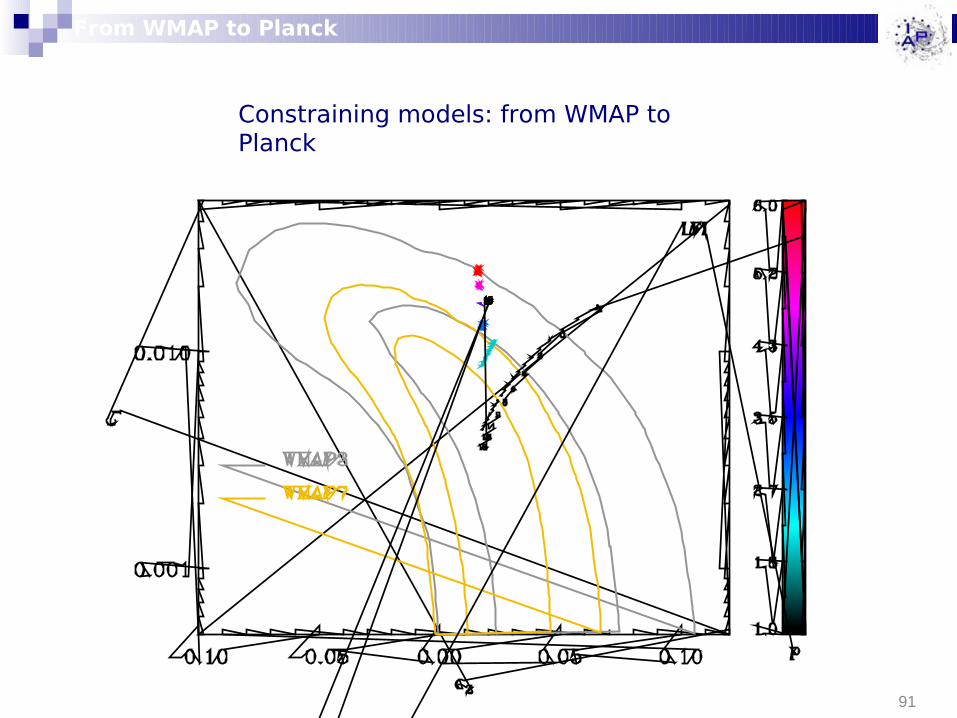
From WMAP to Planck
92
Constraining models: from WMAP to Planck
From WMAP to Planck
93
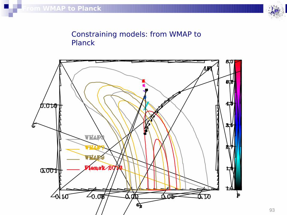
Constraining models: from WMAP to Planck
From WMAP to Planck

Category 1 is the category chosen by Planck
Planck likes category 1
Plateau inflation
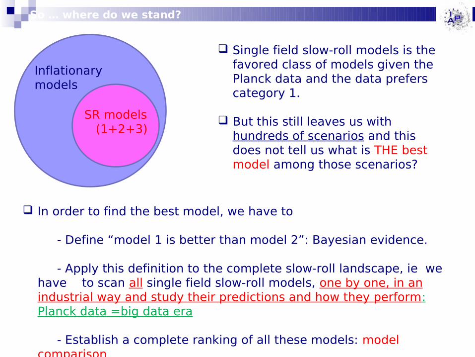
So … where do we stand?
Inflationary models
SR models (1+2+3)
In order to find the best model, we have to
- Define “model 1 is better than model 2”: Bayesian evidence.
- Apply this definition to the complete slow-roll landscape, ie we have to scan all single field slow-roll models, one by one, in an industrial way and study their predictions and how they perform: Planck data =big data era
- Establish a complete ranking of all these models: model comparison
Single field slow-roll models is the favored class of models given the Planck data and the data prefers category 1.
But this still leaves us with hundreds of scenarios and this does not tell us what is THE best model among those scenarios?

arXiv:1303.3787≈ 74 models
≈ 700 slow roll formulas
≈ 365 pages
Encyclopedia Inflationaris
The encyclopedia contains the slow-roll treatment and comparison to the Planck data for all slow-roll models : this is not a review paper!

theory.physics.unige.ch/~ringeval/aspic.html
The ASPIC library provides all the numerical codes for all models
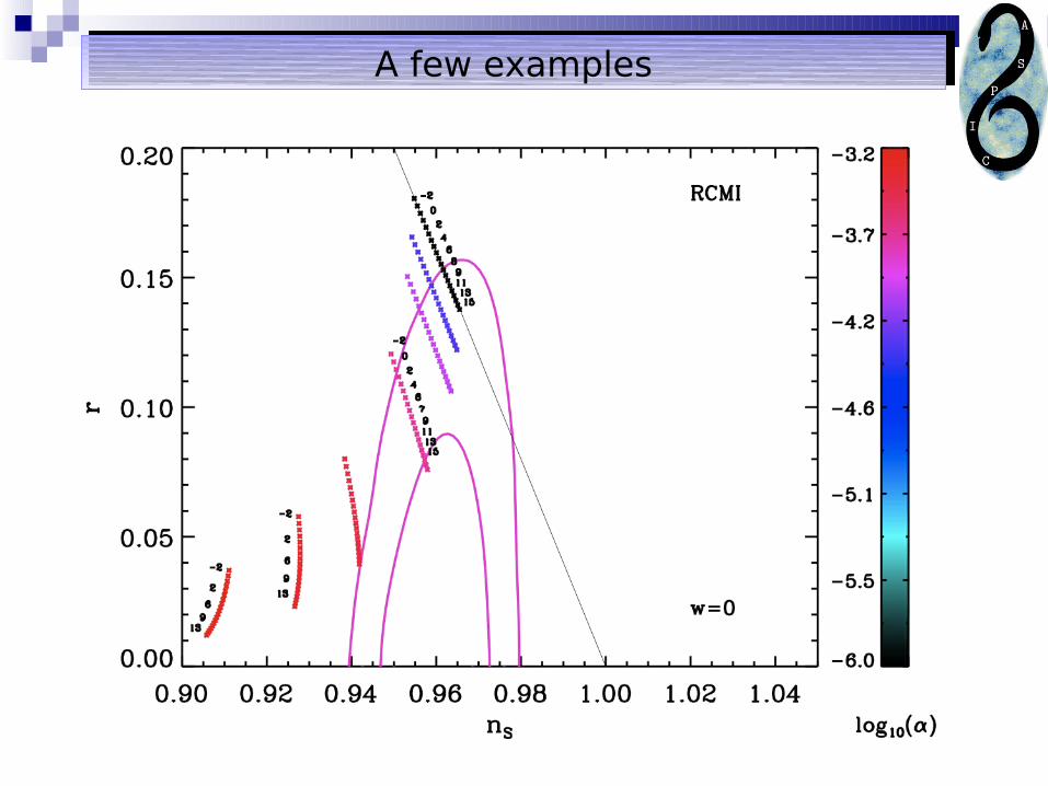
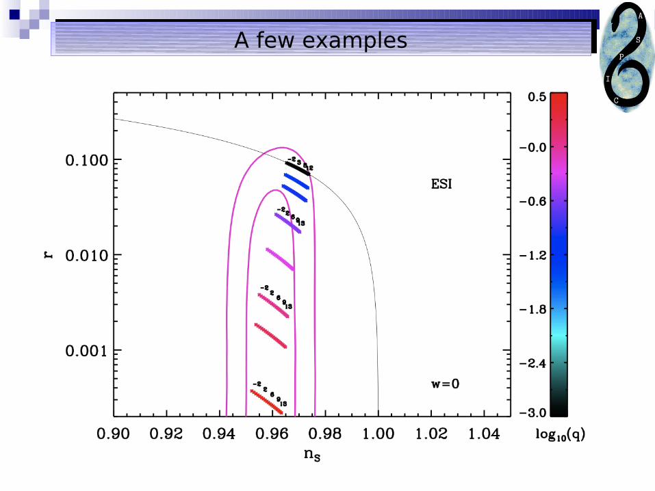
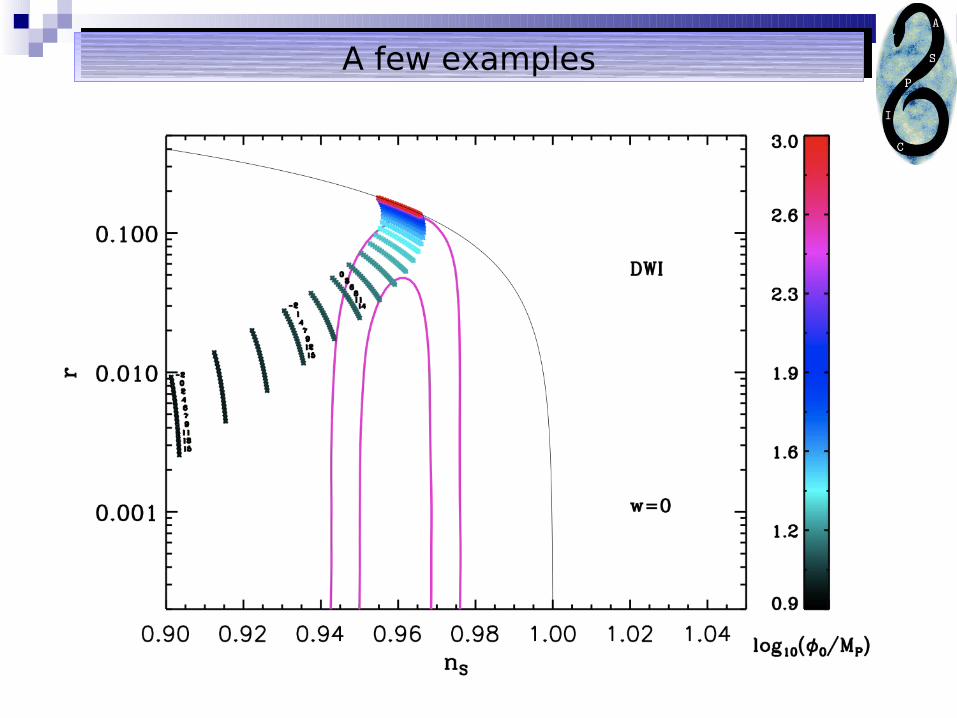
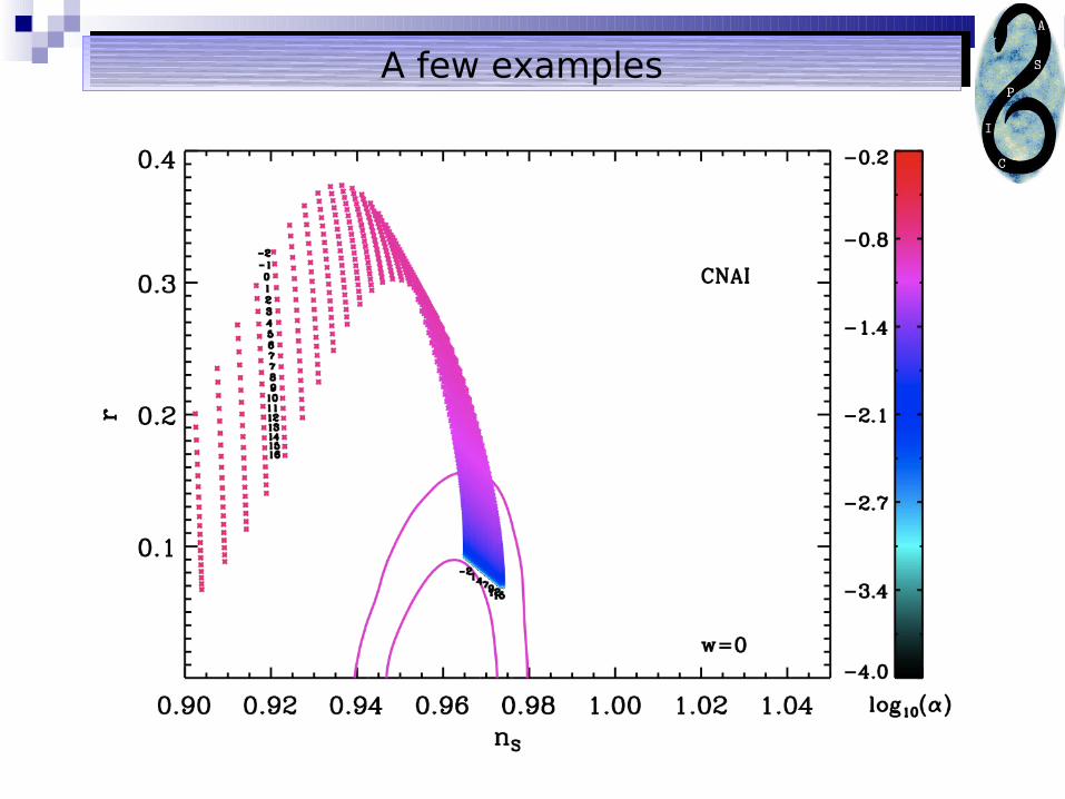
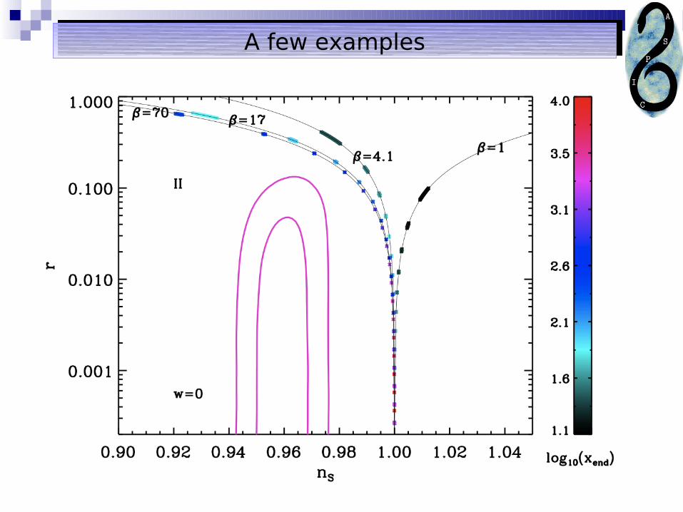
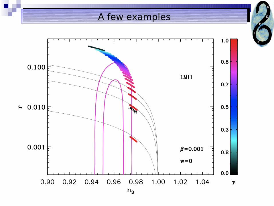
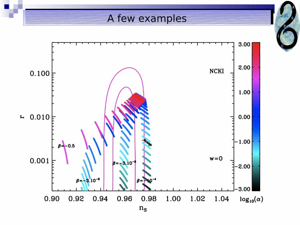
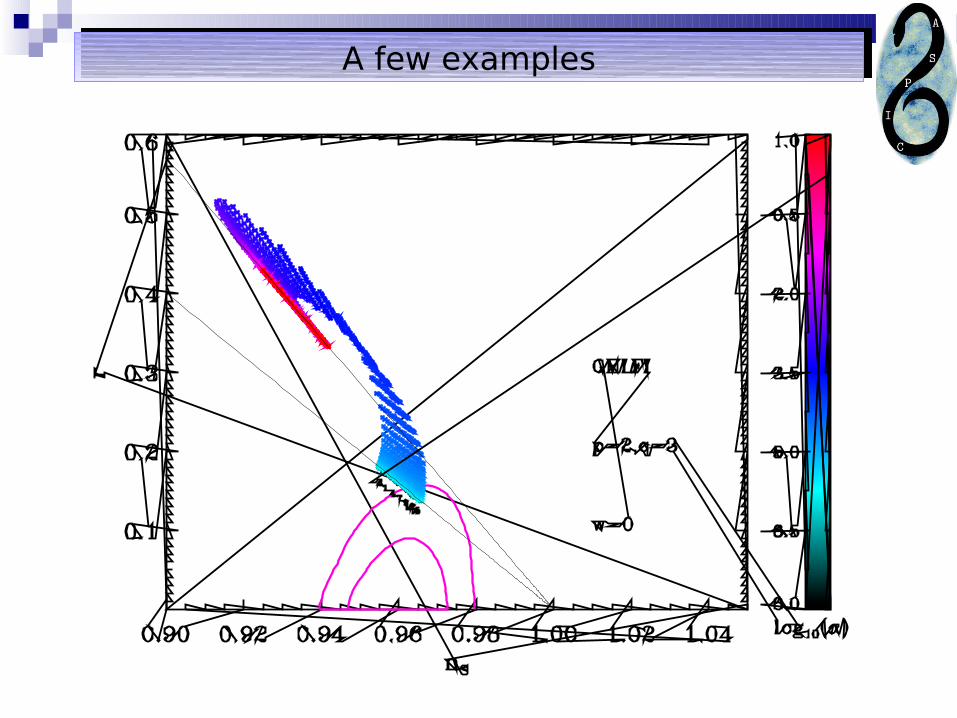
A few examplesA few examples
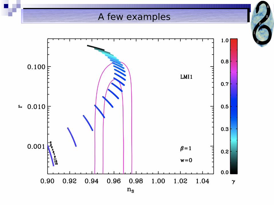
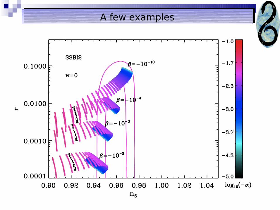
A few examplesA few examples
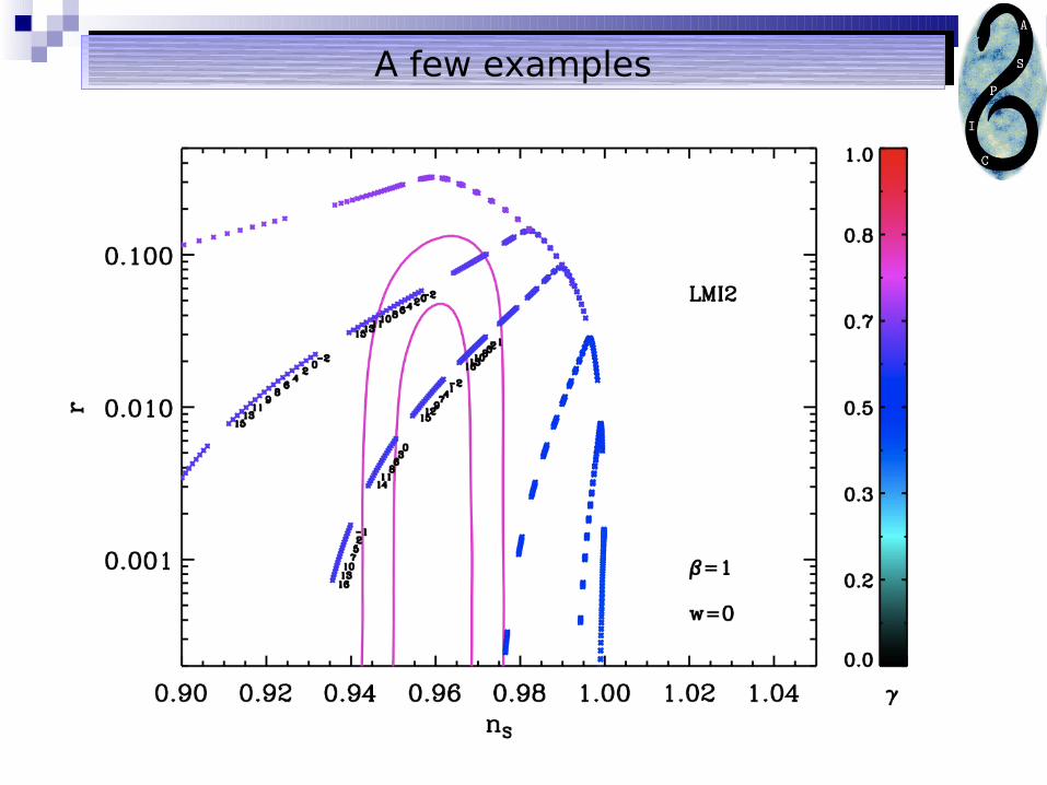
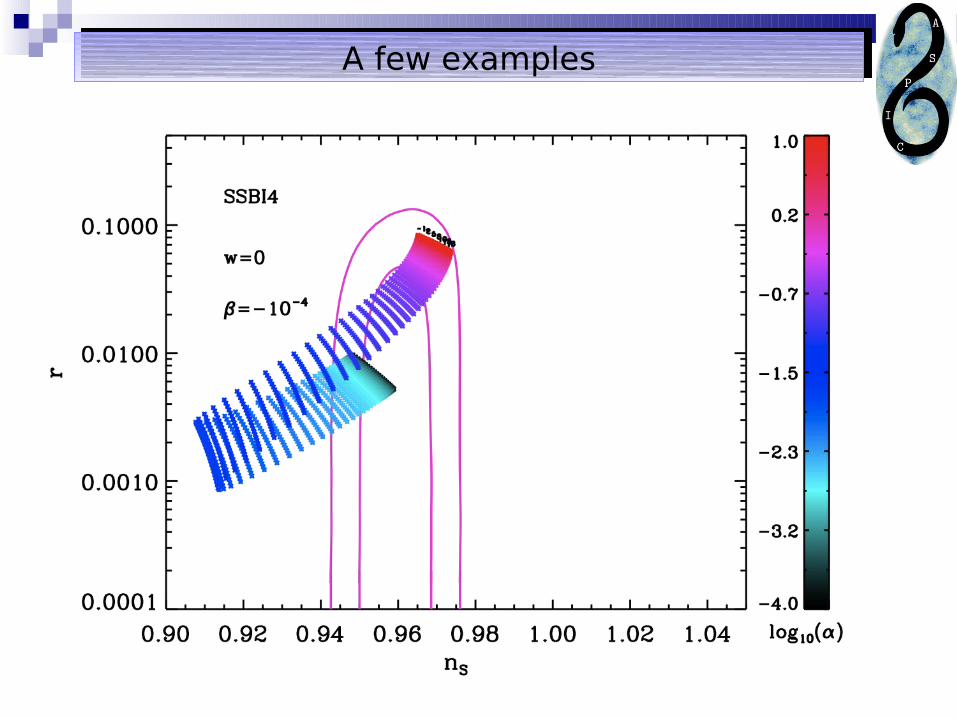
A few examplesA few examples
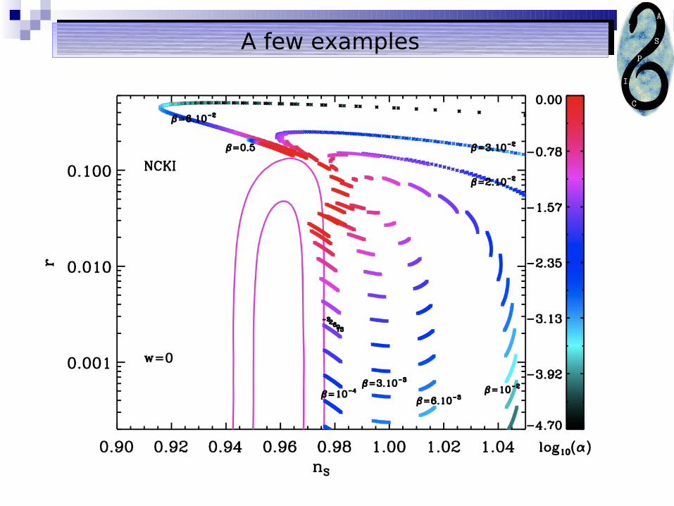
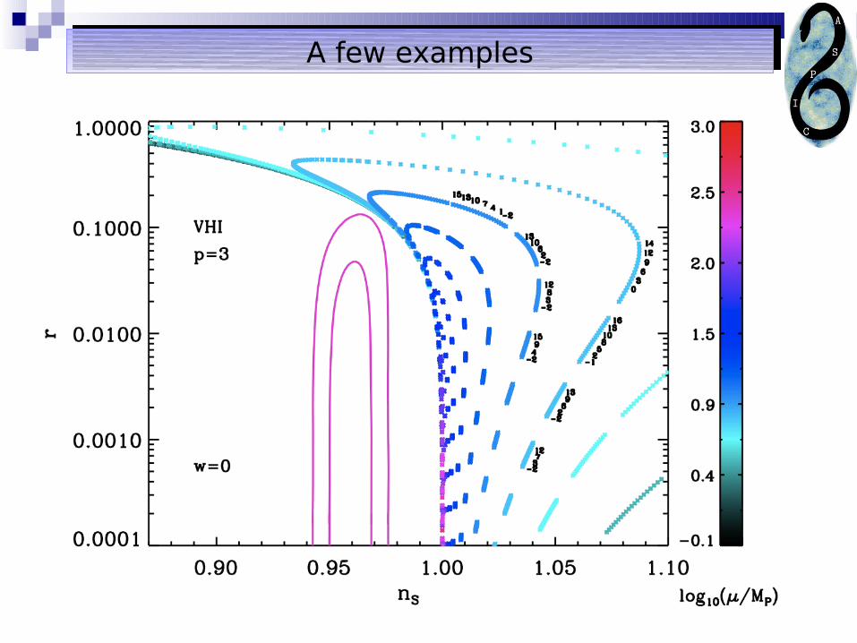
A few examplesA few examples
A few examplesA few examples
A few examplesA few examples
A few examplesA few examples
A few examplesA few examples

A few examplesA few examples
A few examplesA few examples
A few examplesA few examples

A few examplesA few examples
A few examplesA few examples
A few examplesA few examples
A few examplesA few examples
A few examplesA few examples
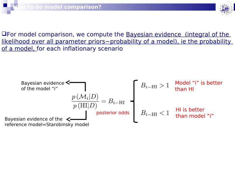
For model comparison, we compute the Bayesian evidence (integral of the likelihood over all parameter priors~probability of a model), ie the probability of a model, for each inflationary scenario
How to do model comparison?
Bayesian evidence of the reference model=Starobinsky model
Bayesian evidence of the model “i”
posterior odds
Model “i” is better than HI
HI is better than model “i”
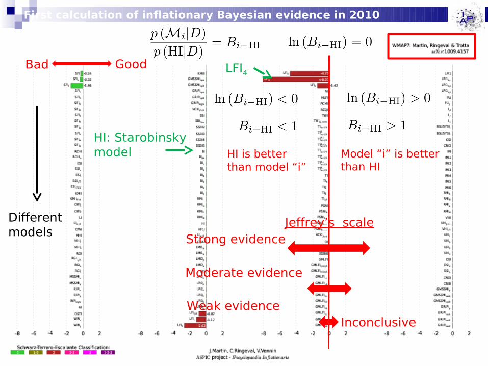
First calculation of inflationary Bayesian evidence in 2010
Model “i” is better than HI
HI is better than model “i”
InconclusiveWeak evidence
Strong evidence
Bad Good LFI4
HI: Starobinsky model
Different models
Jeffrey’s scale
Moderate evidence
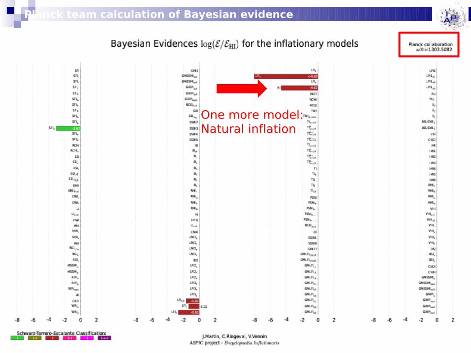
Planck team calculation of Bayesian evidence
One more model: Natural inflation
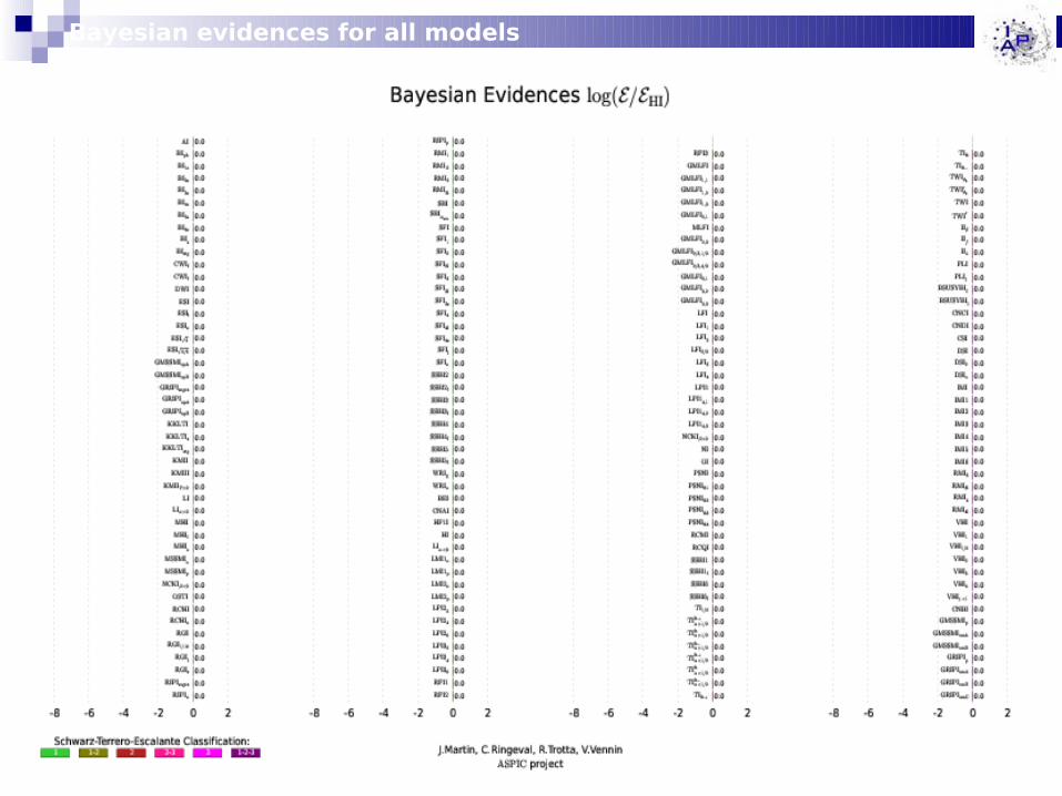
Bayesian evidences for all models

ASPIC evidence: good models
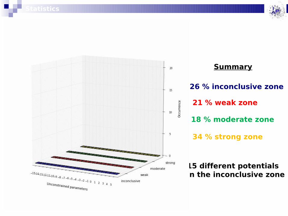
Statistics
26 % inconclusive zone
21 % weak zone
18 % moderate zone
34 % strong zone
Summary
15 different potentialsin the inconclusive zone

And the winners are …
MHI
RGI
KMIII
HI
ESI
SFI
Planck has identified the shape of the inflaton potential:
Plateau inflation
NB: the difference between these modelsis “inconclusive”.
Recap
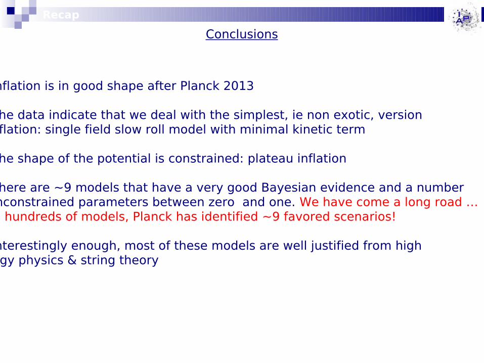
Conclusions
Inflation is in good shape after Planck 2013
The data indicate that we deal with the simplest, ie non exotic, version of inflation: single field slow roll model with minimal kinetic term
The shape of the potential is constrained: plateau inflation
There are ~9 models that have a very good Bayesian evidence and a number of unconstrained parameters between zero and one. We have come a long road … from hundreds of models, Planck has identified ~9 favored scenarios!
Interestingly enough, most of these models are well justified from high energy physics & string theory

And the winners are …