370

Charles University Center for Economic Research and Graduate Education

Academy of Sciences of the Czech Republic Economics Institute

Jana Krajčová

TESTING LENIENCY PROGRAMS EXPERIMENTALLY:

THE IMPACT OF CHANGE IN PARAMETERIZATION

CERGE-EI

WORKING PAPER SERIES (ISSN 1211-3298) Electronic Version

Working Paper Series 370 (ISSN 1211-3298)

Testing Leniency Programs Experimentally: The Impact of Change in Parameterization

Jana Krajčová

CERGE-EI

Prague, October 2008

ISBN 978-80-7343-170-9 (Univerzita Karlova. Centrum pro ekonomický výzkum a doktorské studium) ISBN 978-80-7344-159-3 (Národohospodářský ústav AV ČR, v.v.i.)

Testing Leniency Programs Experimentally:

The Impact of Change in Parameterization∗

Jana Krajcova†

CERGE–EI‡

October 2008

Abstract

I analyze subjects’ sensitivity to parametric change that does not af-fect the theoretical prediction. I find that increasing the value of an illegaltransaction to a briber and reducing the penalties to both culprits leads tomore bribes being paid but does not affect the cooperation of the bribee.My data also suggest that trust and preferences towards others might play arole. My paper provides a testbed for experimental testing of anti-corruptionmeasures and adds evidence to the on-going discussion on the need for socio-demographic controls.

Abstrakt

Analyzujem dopad zmeny parametrov, ktora neovplyvnuje teoreticku pre-dikciu, na rozhodovanie ucastnıkov experimentu. Zistila som, ze zvysenievyplaty plynucej platcovi uplatku z ilegalnej transakcie a sucastne znızeniepenale pre oboch pachatel’ov vedie k zvyseniu korupcie, avsak nema vplyvna d’alsie rozhodovanie prıjmatel’a uplatku. Moje vysledky tiez naznacuju,ze dovera a preferencie voci blahu inych mozu zohravat’ dolezitu ulohu prirozhodovanı. Moj clanok poskytuje vychodiskovy testovacı zaklad pre exper-imentalne testovanie protikorupcnych opatrenı, a tiez prispieva k pokracu-jucim diskusiam o vyzname sociodemografickych charakteristık pri analyzeexperimentalnych dat.

Keywords: corruption, anti-corruption mechanisms, optimal contract, mon-itoringJEL classification: C91, D02, D73, K42

∗My special thanks go to Prof. Andreas Ortmann for consultation on and supervision ofthis research. I would also like to thank Ondrej Rydval, Peter Katuscak, Lenka Drnakova, andespecially Libor Dusek for valuable tips and very helpful suggestions and comments. This studywas supported by GACR grant No. 402/04/0167.

†E-mail: jana.krajcova@cerge-ei.cz‡Center for Economic Research and Graduate Education–Economics Institute, a joint work-

place of Charles University in Prague and the Academy of Sciences of the Czech Republic. Ad-dress: CERGE–EI, P.O. Box 882, Politickych veznu 7, Prague 1, 111 21, Czech Republic.

1

1 Introduction

The severe consequences of corruption have been documented in numerous empir-

ical studies. For example, Mauro (1995) and Tanzi (1998) have shown a negative

effect of corruption on economic growth; Hwang (2002) has demonstrated that cor-

ruption, through tax evasion, reduces government revenues; and Gupta, Davoodi

and Alonso-Terme (2002) have shown that corruption increases income inequality

and poverty. The design and implementation of effective anti-corruption measures

therefore remains an important concern.

One promising anti-corruption measure is the leniency policy. Leniency policies

award fine reductions of varying intensities to wrongdoers who “spontaneously”

report an illegal agreement and thereby help to convict their accomplice(s). They

serve as an enforcement mechanism as much as a means of deterrence in that, if

appropriately designed and implemented, they have the potential to undermine the

trust between wrongdoers. Leniency policies have been analyzed in the literature

mostly as an anti-cartel mechanism.

The deterrence effect of leniency policies in the case of cartels has been analyzed

– and confirmed – both theoretically (e.g. Spagnolo 2004) and experimentally (e.g.

Apesteguia, Dufwenberg and Selten 2004; Bigoni, Fridolfsson, Le Coq and Spagnolo

2007, 2008).

Spagnolo (2004), for example, theoretically examines the effects of leniency

policies of various degrees – from moderate (which reduce or cancel the penalty for

a criminal who reports) to full (which, in addition, pay a reward). He shows that

reward-paying leniency programs provide a (socially) costless1 and very efficient

measure for cartel deterrence.

1This is the case if the rewards are fully financed from fines imposed on other convictedmembers of the cartel.

2

Drawing on earlier versions of Spagnolo (2004), Apesteguia, Dufwenberg and

Selten (2004) conducted an experiment that confirms the promising cartel-deterring

properties of leniency policies. Bigoni, Fridolfsson, Le Coq and Spagnolo (2007,

2008) conducted related experiments. In addition to confirming the basic results

about the effectiveness of leniency programs, they attempted to acquire a deeper

understanding of the driving forces. In several treatments they vary specific features

of the game – fine levels, exogenous risk of detection, reward schemes, possibility to

communicate, and the eligibility for leniency. They control for past convictions and

for subjects’ risk attitudes. The experiments are run in Stockholm and in Rome,

which allows assessing potential cultural effects.

Bigoni et al (2007) find that leniency leads to higher deterrence but at the same

time helps to sustain higher prices. Rewards lead to almost complete deterrence –

which is in line with Spagnolo’s (2004) result. Past convictions reduce the number of

cartels but increase collusive prices. The authors, in addition, distinguish between

two types of past convictions 1) those that occur as a result of reporting and 2) those

that occur as a result of external investigation. They find that past convictions

after reporting have a much stronger deterrence effect than past convictions after

external investigation. The results also confirm a strong cultural effect.

Bigoni et al (2008) focuses on the role of risk attitudes. They find that risk

aversion and the willingness to form a cartel are negatively correlated. The results

suggest that past experience might have more important consequences for the per-

ception of risk than the exogenous probability of detection, and that the strategic

risk (the risk of being cheated upon) plays a key role for the effectiveness of a

leniency policy.

Both Bigoni et al (2007) and (2008) contribute to a better understanding of

the cartel-deterring properties of leniency policies and highlight the importance of

proper policy design.

3

Leniency policies to deter cartels are, however, not directly applicable as anti-

corruption measures, since cartel deterrence is essentially a simultaneous game

while strategies, payoffs, and the move structure of anti-corruption measures are

asymmetric.2 A proper theoretical and experimental analysis is therefore called for.

To my knowledge the first theoretical work analyzing the various effects of le-

niency policies on corruption is Buccirossi & Spagnolo (2006). The authors show

that poorly designed moderate policies may have a serious counter-productive ef-

fect: they might allow a briber to punish at relatively low cost a partner who does

not respect an illegal agreement. In other words, some leniency policies might ac-

tually provide an enforcement mechanism for occasional illegal transactions.3 Thus

they can, contrary to the intention, increase corruption.

Buccirossi & Spagnolo’s result together with the theoretical and experimental

evidence from the literature on cartel deterrence suggests that the potential of

leniency policies to undermine trust between wrongdoers hinges upon proper design

and implementation.

Experimental methods have been widely used, albeit rarely, to study corruption

(Dusek, Ortmann and Lızal 2005). They become especially useful when counter-

factual institutional arrangements such as leniency programs need to be explored:

they provide, for example, relatively cheap ways to examine the effects of such

arrangements in controlled environments (see Dusek et al 2005, Apesteguia et al

2004, Buccirossi & Spagnolo 2006, Bigoni et al 2007, 2008, Richmanova & Ortmann

2008, and also Roth 2002).

In Richmanova & Ortmann (2008) we proposed a generalization of the Buc-

cirossi & Spagnolo (2006) model by introducing the probabilistic discovery of evi-

dence.4 Our generalization makes the model more realistic and more readily appli-

2For a more detailed discussion see Richmanova (2006).3Occasional illegal transactions are essentially one-shot transactions.4In the original model, Buccirossi & Spagnolo assume that the briber and bribee agree to

4

cable for experimental testing without changing the qualitative results of Buccirossi

& Spagnolo.

We use the generalized Buccirossi & Spagnolo model for the experimental testing

of leniency policies as an anti-corruption measure. As we address two different

methodological issues that (anti-)corruption experiments are afflicted with, our

results are reported in two papers: the present paper, and the closely related work

reported in Krajcova & Ortmann (2008). Both papers provide a new testbed for

anti-corruption programs.

Altogether, we design three experimental treatments: a benchmark, which is

common for both studies, Krajcova & Ortmann (2008) and the present paper, and

in which all instructions are presented in completely neutral language; a context

treatment, in which we use the same parameterization as in the benchmark but

instructions are presented in full bribery context (Krajcova & Ortmann 2008);

and a high-incentive treatment, which implements a new parameterization within

neutral framing (the present paper).5

In Krajcova & Ortmann (2008), following the earlier work of Abbink & Hennig-

Schmidt (2006), we study the effect of“loaded”instructions in a bribery experiment.

Surprisingly, Abbink & Hennig-Schmidt find no significant impact of instructions

framing. The authors conclude that this result may be caused by the nature of

the game: it is very simple, and as it was designed to capture all the basic fea-

tures of bribery, even with neutral wording, subjects may have deciphered what

the experiment was about. Our bribery game includes stages where players can

report their opponents and receive leniency, which makes it more complex and also

produce hard evidence, which serves as a hostage. Without hard evidence being produced, theoccasional illegal transaction is not enforceable. An audit, if it takes place, discovers the evidencewith a probability of one. In Richmanova & Ortmann (2008), we argue that instead some evidenceis created unintentionally and this can be discovered by an audit with some probability that isless than one.

5We have, in addition, designed some additional exploratory treatments which we use for arobustness check of the main results. See the appendix for more details.

5

potentially more susceptible to the non-neutral context. Therefore, it calls for a

separate analysis. We find a strong gender effect - male and female participants

react differently to the non-neutral context. The effect of context becomes signifi-

cant once we allow for gender-specific coefficients. Thus, in contrast to the results

of Abbink & Hennig-Schmidt (2006), we find that a bribery context indeed makes

a (significant) difference.

In the present paper I study the effect of a change in parameterization. It has

been documented in the literature that a change in parameterization that does not

affect the theoretical prediction might indeed have consequences for the behavior

of subjects in the lab (see e.g. Goeree & Holt 2001). Anti-corruption experiments

might be particularly tricky, being sensitive to changes in design. In the generalized

Buccirossi & Spagnolo game, the action bringing the highest possible payoff is also

associated with a risk of considerable loss. Therefore, risk or loss attitudes are

also likely to play a role. Altogether, I expect that subjects in the lab might not

behave in accordance with the theoretical prediction, especially when the prediction

is made under an assumption of risk neutrality.6 The question I ask is whether

by making corruption more attractive by i) increasing the potential gain and ii)

reducing the penalty if bribery is discovered, I can induce more corruption in the

lab even if the theoretical prediction suggests no change. I also study to what

extent the subjects’ decisions in the experiment can be explained by their basic

socio-demographic characteristics.

I do indeed find a significant effect of parametric change. Even though the

change I implemented has no consequences for the theoretical prediction, I observe

much more corruption in the high-incentive than in the benchmark treatment. My

data suggest that trust and preferences towards others might play a role. The econo-

metric analysis provides limited evidence on the role of basic socio-demographic

6In fact, in our data we observe deviations from the theoretical prediction in all three treat-ments.

6

characteristics. I find no differences in how the parametric change affects the be-

havior of male and of female participants. Our papers provide a testbed for the

experimental testing of anti-corruption measures and add evidence to the on-going

discussion on the need for socio-demographic controls.

The remainder of the paper is organized as follows. In the next section I dis-

cuss the generalized Buccirossi & Spagnolo model in detail, and I also describe

and compare two experimental treatments. Section 3 talks about experimental

implementation and in Section 4 I review the results. Section 5 concludes.

2 Experimental Design

The experiment implements the bribery game in Richmanova & Ortmann (2008).

An entrepreneur has an investment possibility of net present value v, if a bureaucrat

is willing to perform an illegal action, Action a. For doing so, the bureaucrat may

require compensation in the form of a bribe, b.

The timing of the game is as follows. First, the entrepreneur decides whether

to Pay or Not Pay a bribe. If she does not pay a bribe, the game ends. If she does,

the bureaucrat chooses one of three possible actions: Denounce, do Nothing,7 or

perform Action a.8

If the bureaucrat chooses Denounce, an audit is carried out. The audit may

(with probability β, β ∈ (0, 1)), or may not (with probability 1 − β), discover

some evidence of bribery. If the bribery attempt is detected, the leniency policy

7Nothing denotes a passive action choice. For the bureaucrat, it means that he neither de-nounces nor respects (by providing the favor) the illegal agreement. For the entrepreneur, itmeans that she does not denounce in response to the bureaucrat’s action.

8Action a means that the bureaucrat respects the illegal agreement and thus provides an(illegal) favor to the entrepreneur. That is, strictly speaking, not a corrupt action because itdoes not impose a negative externality on the public. According to Abbink, Irlenbusch & Renner(2002) it is not such a problem since people do not care much about the costs they impose onothers.

7

guarantees that the bureaucrat will have to pay only a reduced fine whereas the

entrepreneur will have to pay the full fine. In addition, bribe b is confiscated.9 If

the bribery is not detected, the bureaucrat will enjoy bribe b.

If the bureaucrat chooses Nothing or Action a, the entrepreneur has another

move. In both cases, she may choose between Denounce and do Nothing.

If the entrepreneur chooses Denounce and the ensuing audit discovers evidence

(which, again, happens with probability β), then she will have to pay a reduced

fine whereas the bureaucrat will have to pay the full fine and, in addition, their

illegal gains will be confiscated. If no evidence is discovered, both the bureaucrat

and the entrepreneur will keep their illegal gains.

If the entrepreneur chooses Nothing, then an audit may still occur with some

nonzero probability α. If the audit detects bribery (which happens with probability

β), both parties are subject to a sanction, which consists of the confiscation of the

illegal gains plus the full fine. The illegal gains include bribe b in any case and

value v only in the case when the bureaucrat has chosen to perform Action a.

Figure 1 below summarizes the extensive form of the game and the expected

payoffs.

The contribution of the generalized model lies in the introduction of probability

β. In Buccirossi & Spagnolo (2006) it is assumed that, before the illegal transaction

takes place, the bureaucrat and the entrepreneur agree on the production of hard

evidence. Without hard evidence being voluntarily produced by both of them the

illegal transaction is not enforceable. In essence it is assumed that both involved are

holding a hostage that commits each other to the desired outcome. It is furthermore

assumed that, if an audit takes place, corruption is discovered and both culprits

are convicted with a probability of one. Richmanova & Ortmann (2008) assume

9Note that in this case the illegal transaction has been detected without Action a being per-formed and therefore there is no gain to the entrepreneur to be confiscated.

8

Figure 1: Extensive form of the corruption game in the generalized model. P stands for Pay, NPfor Not Pay, D for Denounce, N for doing Nothing, a for performing Action a, b for bribe, v forthe value of the project to the entrepreneur, α for the exogenous probability of an audit, β forthe probability of conviction, FE and FB for full fines and RFE and RFB for reduced fines to theentrepreneur and to the bureaucrat, respectively.

instead that some hard evidence is created unintentionally along the way and that

this evidence may be discovered by an audit with probability β ∈ (0, 1). The basic

structure of both the original and the modified game is the same except that in the

original version the probability β is set to 1. The generalization makes the model

more suitable for experimental testing, as no additional stage is needed in which

subjects would have to agree on producing a hostage. In addition, the generalized

model arguably resembles real-world situations more closely.10

Buccirossi & Spagnolo (2006) show that in the absence of a leniency program,

occasional illegal transactions are not implementable.11 The result carries over into

10I realize that in such a game beliefs about the probability of detection might play an importantrole. However, I believe that the introduction of beliefs would make the game more complex thannecessary for experimental testing. Instead, I view probability β as an empirical success rate, oreffectiveness, of a detection technology that is known to subjects.

11Facing the full fine even after reporting, the entrepreneur cannot credibly threaten to reportthe bureaucrat in the case when he would not deliver. Therefore, the bureaucrat would keep thebribe and not perform Action a, knowing that it is not profitable for the entrepreneur to punishhim. Consequently, the entrepreneur would not enter the illegal agreement in the first place.

9

the generalized model. After the introduction of a modest leniency program,12

occasional illegal transactions are enforceable if the following three conditions are

satisfied simultaneously. First, the no-reporting condition for the bureaucrat: the

reduced fine must be such that the bureaucrat prefers performing Action a to

Denouncing once the bribe has been paid. Second, the credible-threat condition

for the entrepreneur: the reduced fine and the full fine must be set such that the

entrepreneur can credibly threaten to report if the bureaucrat does not deliver.

Third, the credible-promise condition: the entrepreneur must be able to credibly

promise not to report if the bureaucrat respects the illegal agreement.

These three conditions, given the value of the project together with the full

and reduced fines, define a bribe range for which the occasional illegal transaction

is implementable. Even though these conditions are modified in the generalized

model, the qualitative result remains unaffected.

I used the generalized version of the game for experimental testing of the the-

oretical prediction under two different scenarios: when the occasional illegal trans-

action is implementable in equilibrium, and when it is not. Implementability is a

function of the per-round endowment for the entrepreneur. The per-round endow-

ment exogenously defines the value of the bribe if the entrepreneur decides to pay

it.13 For each treatment I use two possible values of the per-round endowment: a

low endowment that theoretically leads to a no-corruption equilibrium, and a high

endowment that theoretically leads to a corruption equilibrium.

I want to study whether a change in parameterization that does not affect the

theoretical prediction will have an impact on the behavior of subjects in a lab.

In a game like this, where an action bringing the highest possible payoff is also

12Similarly to Spagnolo (2004), “modest” means that a leniency program does not reward forreporting, at best it cancels the fine.

13This way I reduce the cognitive demand on subjects: the only decision they have to make iswhether they want to transfer their per-round endowment or not.

10

associated with the risk of an enormous loss, it is likely that subjects in the lab

will not behave in full accordance with the theoretical prediction. I want to see

whether by making the risky choice more tempting I can induce more transferring

in the lab. I also want to see what the consequences are for later stages of the game,

particularly for denouncing. For that purpose I ran two treatments: a benchmark

and a high-incentive treatment.

Table 1 below summarizes the parameterizations chosen for the Benchmark

treatment (B) and for the (Benchmark-)High-incentives treatment (BH).

Treatment α b v RFE RFB FE FB EL EH show-upB 0.1 0.2 100 0 0 300 300 20 40 300BH 0.1 0.2 200 0 0 200 200 10 30 200

Table 1: Experimental parameterization. α and β denote the probability of an audit and ofdiscovering evidence of bribery, respectively; v denotes the value of the project to the entrepreneur;RFE and RFB denote reduced fines and FE and FB full fines to the entrepreneur and to thebureaucrat, respectively; EL and EH denote low and high per-round endowment, respectively;show-up stands for the show-up fee.

In the B treatment, the probabilities α and β were chosen such that they approx-

imately correspond to real-world exogenous probabilities of audit and to real-world

conviction rates; at the same time they are intuitively comprehensible for subjects.

The value of the project v was chosen together with full fines FE and FB such that

the subject faces a considerable gain from the investment but also severe punish-

ment in the case of detection. I set reduced fines RFE and RFB equal to zero to

analyze the case of full leniency programs which, according to Apesteguia et al

(2004), have promising anti-cartel properties. Endowment determines the value of

a bribe to (not) be paid. The “low endowment” of 20 leads (theoretically) to no

corruption, whereas the “high endowment” of 40 leads to corruption equilibrium.

Finally, the show-up fee was set such that I eliminate the possibility of earning a

negative total from the experiment.

In the BH treatment, in order to make the risky but high-payoff choice more

11

tempting, I increased the value of the project to the entrepreneur and, at the

same time, I reduced the fines both agents face in case of detection. I keep the

probabilities of detection and of conviction (thus the exogenous risk) unchanged.

In order to keep the theoretical prediction for low- and high-endowment periods

qualitatively the same as in the benchmark treatment, the per-round endowments

were also adjusted. Finally, the show-up fee is set such that subjects cannot end

up with a negative final payoff, but there is a chance that they will earn zero.

The extended game forms together with the expected payoffs resulting from the

parameterizations for both the B and the BH treatments are illustrated in Figure 2

for low- and for high-endowment periods. The branches identifying the equilibrium

choices of risk-neutral agents are in bold.

Figure 2: Expected payoffs from the corruption game in the B (benchmark) and the BH (high-incentive) treatments, respectively. Rows in the tables correspond to Participant X and Partici-pant Y; columns correspond to the B and BH treatments. The theoretical prediction is the samefor both treatments, it only varies with the endowment.

12

3 Implementation

The experiment was conducted in November and December 2006 at CERGE-EI in

Prague, using a mobile experimental laboratory.14

Participants were recruited from the Faculty of Social Sciences of Charles Uni-

versity in Prague and from various faculties of the Czech Technical University in

Prague. Students were approached via posters distributed on campus and via e-

mail.15

I conducted four sessions of each treatment. Twelve participants, six in a role

of Participant X – the entrepreneur – and six in a role of Participant Y – the

bureaucrat – interacted in each session. In each session, all subjects participated

in six rounds during which they kept the role that was assigned to them at the

beginning of the first round.16 Participants were randomly and anonymously re-

matched after each round so that no subject was matched twice with the same co-

player. This was common knowledge. The incentive compatibility of this matching

scheme is discussed in Kamecke (1997).

Table 2 summarizes the demographic characteristics of subjects participating in

the experiment. The majority of my subjects were male, reflecting the composition

of the subject pools that I drew on. Mean age ranges between 20.9 and 22.9, over

all sessions the minimum is 18 and maximum 27. I also measured subjects’ risk

14http://home.cerge-ei.cz/ortmann/BA-PEL.htm15By email, I also directly invited students who participated earlier in unrelated experiments

conducted at CERGE-EI.16After each Participant X interacted exactly once with each Participant Y, the roles were

switched for another six rounds. Subjects were not informed about the switch of roles in advancein order to avoid a possible impact on their behavior in the first six rounds. Before the beginningof the seventh round the announcement about the switch of roles appeared on their screens. Thedecisions in the last six rounds are likely affected by subjects’ experience from the first six roundsand therefore I do not report them in the main text. A comparison of the before-switch andafter-switch data is provided in the appendix. For the B treatment, I observe more transferringin the after-switch data, and also more denouncing in both the second and the third stage. Inthe BH treatment, I observe less denouncing in the second stage. The rest of the results seemsunaffected.

13

aversion using a questionnaire based on Holt & Laury (2002). Mean RA score

ranged between 24.8 and 34.7, over all sessions the minimum is 15 and maximum

51.17 Average final payoffs for the B treatment ranged from 320 to 330, with the

minimum being 300 and the maximum 400; for the BH treatment it ranged between

185.8 and 309.2, with the minimum being 018 and the maximum 400.19

Treatment SubjectSource20

M/Fratio21

mean(age)

mean(RA score)

mean(final pay)22

Irreg23

B FSS 8/4 20.9 29.7 320 1B FSS 10/2 21.75 28.8 330 0B CTU 11/1 22.9 34.7 330 0B FSS 9/3 22.3 26.4 323.3 0BH CTU 9/3 22.6 33 185.8 1BH CTU 10/2 22.8 28.9 309.2 0BH CTU 10/2 22.5 29.3 241.7 1BH FSS 10/2 21.9 24.8 259.2 1

Table 2: Summary of the demographic characteristics of subjects for all eight sessions.

Each session began with general instructions. Afterwards, subjects were asked

to fill in Risk-aversion and Demographic questionnaires, for which they earned

their show-up fee. Then the instructions to the computerized part of the exper-

iment were distributed. Understanding of the instructions was tested by a brief

17The higher the score the more risk averse the subject is. The maximum possible RA scoreis 60 which, using the standard CRRA utility function x(1−r), approximately corresponds to arelative risk aversion coefficient of .17. The minimum possible RA score is 0, which approximatelycorresponds to a relative risk aversion coefficient of −.13. An RA score of 23 corresponds to risk-neutrality.

18At that point 400 CZK corresponded to about 16 USD, in purchasing power up to twice asmuch. Subjects were informed during recruitment that their final payoff from the experimentmight be zero, but could not be negative. The non-negativity of the final payoff was ensured bythe show-up fee.

19The difference in average payoffs in the B and in the BH treatment results from differentparameterization as well as from different behavior of subjects as will be illustrated later.

20For each session, subjects were recruited from one source. FSS stands for the Faculty of SocialSciences in Prague, CTU for the Czech Technical University in Prague. I control for imbalanceof the subject pool by including the econ and gender dummies in the econometric analysis.

21Male/Female ratio in the session.22This is the average final payoff after the computerized part of the experiment.23Irreg stands for a dummy variable for session irregularities. In the first B-treatment session

an experimenter effect is possible; in the first BH-treatment session a typo in the Z-tree programcaused incorrect payoffs for two final nodes displayed on the screens, which was pointed out byone of the subjects only after several rounds; in the third BH-treatment session two subjectscontinued communicating despite several admonitions; and in the fourth BH-treatment sessiontwo subjects were reading a newspaper in between making their choices. I do not believe thatthese would matter but wanted to control nevertheless. After running the preliminary regressionsI concluded that they indeed did not matter.

14

questionnaire. The computerized part of the experiment started only after every

participant answered all testing questions correctly.24 The session concluded with

a final questionnaire asking for the subject’s feedback on the experiment.25

All instructions were read aloud by the experimenter. As a part of the in-

structions subjects received a pictorial representation of the game with a minimum

use of game-theoretic terminology. Probabilistic outcomes were presented in both

probabilistic terms and frequency representation (see e.g. Gigerenzer & Hoffrage

1995, or Hertwig & Ortmann 2004). All instructions were presented in completely

neutral language, with no reference to bribery. The roles of the bureaucrat and

the entrepreneur were renamed Participant X and Participant Y, actions were la-

belled with neutral letters, Pay/Not Pay a bribe was replaced with transfer/not

transfer ; and no detection/detection were labelled outcome A and outcome B, re-

spectively (for an analysis of the impact of loaded instructions see e.g. Abbink 2006

or Krajcova & Ortmann 2008).26

The experiment was computerized using Z-tree software (Fischbacher 2007). At

the beginning of each round, each participant was notified of her/his role. Partici-

pants X also learned their current per-round endowment. Then each pair interacted

sequentially.27 Between the second and the third stage, Participants X were asked

about their choices in each node of the third stage if they were to reach it. After

they made their conditional choices, they learned the actual decision of their co-

player and they were asked to confirm, or to change, their previous choice. This

mechanism allowed me to collect some additional data in rounds when the third

stage was not reached.

24This was common knowledge.25For filling out this last questionnaire, subjects were paid an additional 50-200 CZK (corre-

sponds to about 2-9 USD) - the amount varied between sessions. This mechanism was used toadjust average earnings for the session to the level promised during the recruitment.

26Originals (in Czech) of all materials that subjects received during the experiment are availableat http://home.cerge-ei.cz/richmanova/WorkInProgress.html.

27Choices were made by clicking the respective buttons on the screen. Subjects were notifiedthat once they make their choice it would not be possible to take it back.

15

At the end of each round subjects were given feedback about their action(s),

the action(s) of the player they were paired with, the realization of the random

outcome (A or B) and their resulting payoff. At the end, one round was randomly

chosen to determine the final payoff from the computerized part of the experiment.

This mechanism was chosen in order to ensure that the decision in every round is

made as if in a one-shot game. This payment procedure was common knowledge

ex ante.

Participants were paid anonymously in cash right after each session. I used the

Czech crown as the currency unit throughout the whole experiment.

4 Results

In Figure 3 below, the results from low- and high-endowment periods are presented.

Each figure integrates the results from both treatments – the B treatment data in

the upper rows, the BH treatment below. The equilibrium choices for each case are

in bold face.

For the aggregate first-stage data, a clear treatment effect can be observed –

the frequencies of choosing Pay are higher in the BH treatment than in the B

treatment. In both treatments, the frequencies of choosing Pay are higher in the

low-endowment periods than in the high-endowment periods, which contradicts

the theoretical prediction. Intuitively, subjects seem to be willing to transfer their

endowment in order to get a chance of receiving a high payoff, but they are more

willing to put at stake a low endowment than a high. Instead of risking the high

endowment they seem to prefer choosing the sure outcome.

As for the second-stage data, only relative percentages can be compared across

treatments, as different numbers of subjects actually entered this stage of the game.

In both low- and high-endowment periods, the results for the two treatments are

16

Figure 3: Experimental results. For each branch of the extensive form of the game, the upperrow always displays the frequency of the action in the B treatment; and the lower row displaysthe frequency of the action in the BH treatment (both with the corresponding percentage inparentheses). For the nodes E1 and E2, above the branches, I present the conditional choicessubjects were asked to report before they made their actual choice. Frequencies of real choices,which depend on the preceding decision of Participant Y, are presented at the bottom part ofeach figure.

very similar: it is about an equal split between playing Denounce or Action a. Only

in low-endowment periods of the BH treatment Action a slightly dominates. These

results are not in line with the theoretical prediction. The difference in expected

payoffs resulting from Denounce and Action a is, however, very small and that

may be the reason why I do not observe a stronger inclination to either choice.

Also note that in both treatments Denounce is the only action through which the

bureaucrat can avoid a negative expected round payoff with certainty.28 In line

with theoretical prediction and also intuition, Nothing was almost never chosen.

As for the third-stage data, conditional choices provide mixed evidence. In the

E1 node, both conditional and sequential choices in the BH treatment are closer

to the theoretical prediction than in the B treatment. In the E2 node, it is just

28See Figure 2 and Table 1 for more details. Even though the subject could possibly earn anegative round payoff, each subject also received a show-up fee that ensured a non-negative totalpayoff.

17

the opposite: in the BH treatment both conditional and sequential29 choices move

further away from the theoretical prediction.

Note that for the second and third stage data I have too few independent obser-

vations (especially so for the B treatment and for the high-endowment periods)30

to perform a reliable formal analysis. Therefore, I only perform statistical and

regression analysis of the first-stage data.

Analysis of the first-stage data

In the following two subsections I report the results from the formal analysis

of the first-stage data. I conducted standard non-parametric tests identifying dif-

ferences in the distribution of choices under the two treatments. I also computed

the effect size indices to measure the magnitude of the treatment effect. Finally,

I report the results from the estimation of a linear probability model in which I

control for some demographic characteristics of subjects.

Due to the panel nature of the data, I considered four different approaches to

formal regression analysis: 1) clustered data analysis – data from periods 1, 3, and

5 (low-endowment) and from periods 2, 4, and 6 (high-endowment) are clustered

by subject to correct standard errors for likely within-subject correlation; 2) first-

period data analysis – only first-period data (for the low-endowment case) and only

second-period data (for the high-endowment case) are analyzed; 3) averaged data

analysis – averaged data for periods 1, 3, and 5 and for periods 2, 4, and 6 are

analyzed; and 4) dominant-choice data analysis – for each endowment value (low

or high) each subject makes choices in three periods, and the dominant choice is

29When I asked subjects to make their real sequential choices, only one subject in the B treat-ment changed her/his decision in the E2 node from Denounce to Nothing (after observing whatPlayer 2 had chosen) in the low-endowment period. No one changed her/his decision in thehigh-endowment period or in the BH treatment.

30Recall that Figure 3 presents the aggregated data from all the relevant periods, therefore itcontains repeated observations for individual subjects

18

the one that is played more often.

Clustered data have the advantage of using all the available information, while

the other three approaches use only a part of the available information. Therefore,

in the main text I discuss the results for clustered data. The analysis of averaged,

first-period, and dominant-choice data can be found in Appendix 2, part A, as a

robustness check of the main results. By and large, there are no major findings in

these robustness tests.

In addition to the robustness checks based on different “data handling” I also

run a few additional exploratory sessions of treatments in which the experimental

conditions are only slightly modified compared to the benchmark and the high-

incentive treatments. The results from the analysis on the extended data set is

provided in Appendix 2, part B, as an additional robustness check of the main re-

sults. By and large, there are no major findings in these robustness checks. Pooling

slightly different treatments leads to noisier results, which is not very surprising.

4.0.1 Statistical analysis

In Table 3 below I report the results of three standard non-parametric tests in order

to identify the differences in the distributions of choices under the two treatments.

Specifically, I test the null hypothesis of no differences between the two treatments

using the averages of the binary transfer variable31 over periods 1, 3, and 5 and 2, 4,

and 6. According to Wilcoxon rank-sum, Kolmogorov-Smirnov and Fisher’s exact

tests I reject the hypothesis of no differences in the distribution of choices under

two treatments at the 5% significance level.

31Transfer has a value of one if Participant X chooses Pay and a value of zero if s/he choosesNot Pay in the respective period.

19

periods Ranksum32 Ksmirnov33 Fisher34

1,3,5 -3.632(.000)

.500(.002)

(.001)

2,4,6 -3.853(.000)

.625(.000)

(.000)

Table 3: Non-parametric tests.

To assess the magnitude of the effect for practical purposes, I in addition com-

pute two standardized measures of effect size: Cohen’s d and odds ratio, again,

using the averages of the binary transfer variable over periods 1, 3, and 5 and 2, 4,

and 6. The results for the full sample and for the male and female subsamples are

reported in Table 4 below.

B BH effect sizePeriods Sample N mean std.dev. N mean std.dev. odds ratio Cohen’s d1,3,5 full 24 .528 .4495 24 .944 .2123 1.788 1.1827

male 18 .519 .4461 19 .930 .2378 1.792 1.150female 6 .556 .5018 5 1 0 1.799 1.251

2,4,6 full 24 .222 .3764 24 .681 .3330 3.068 1.2924male 18 .296 .4105 19 .719 .3194 2.429 1.150female 6 0 0 5 .533 .3801 NA35 1.983

Table 4: Effect-size indices.

Cohen (1998) defines effect sizes of d = 0.2 as small, d = 0.5 as medium, and

d = 0.8 as large. For the full sample, as well as for the male and female subsamples,

the results suggest a large effect – the transfer rates in the BH treatment are

considerably higher than in the B treatment for both male and female subsamples.

Altogether, both statistical tests and effect-size measures suggest that there are

significant differences between the first-stage choices in the BH and B treatments.

In the next step I perform a further analysis in which I control for gender and for

other subject characteristics.

32Ranksum stands for the two-sample Wilcoxon rank-sum (or Mann-Whitney) test. I reportthe normalized z statistic and corresponding p-value below.

33Ksmirnov stands for the Kolmogorov-Smirnov test. I report the statistic and below the cor-responding p-value from testing the hypothesis that average transfer is lower in the B treatment.

34Fisher stands for Fisher’s exact test. I report the resulting p-value.35A division-by-zero problem occurs, due to no variation in this subsample.

20

4.0.2 Econometric analysis

During the experiment I distributed several questionnaires in order to collect basic

demographic data. Specifically, I have information about subjects’ age, gender,

university and field of study.36 I also measured each subject’s risk aversion.

The dependent variable was defined as a 0/1 dummy variable translog identi-

fying Pay being chosen (value of 1) or not (value of 0) in a particular period. I

estimate a clustered linear probability model. I prefer a linear probability model

to other non-linear alternatives, as it does not rely on very specific distributional

assumptions, the violation of which leads to inconsistent estimates if non-linear

models are employed. Another advantage of the linear probability model lies in the

straightforward interpretation of the estimated coefficients. I run clustered robust

estimation to correct standard errors for likely within-subject correlation and for

heteroskedasticity.

In the appendix, I provide a discussion of the robustness checks I conducted in

addition to the clustered regressions analysis. As the theoretical prediction differs

for low- and high-endowment periods,37 these two groups were analyzed separately.

36In addition, I collected data on: size of subject’s household, number of cars in the house-hold, and whether the subject himself has his own car and what is its approximate value, all ofwhich serve as proxies for income. I also asked the subjects whether they considered themselvesas technical types compared to their peers. I recorded the occurrence of any inconsistencies inthe after-instructions questionnaire, which served as a simple test of understanding of the basicstructure of the game, and in the risk-aversion questionnaire. At the end of the session I asked mysubjects whether they understood the experiment. Finally, I recorded some general informationabout each session – the time of day it started and any session irregularities if they occurred. Afterrunning some preliminary regressions I, however, conclude that none of these variables is signifi-cant for explaining subjects’ decisions. The demographic and the risk-aversion questionnaires arebased on Rydval (2007).

37Recall that in periods 1, 3, and 5 the endowment was low and in periods 2, 4, and 6 theendowment was high.

21

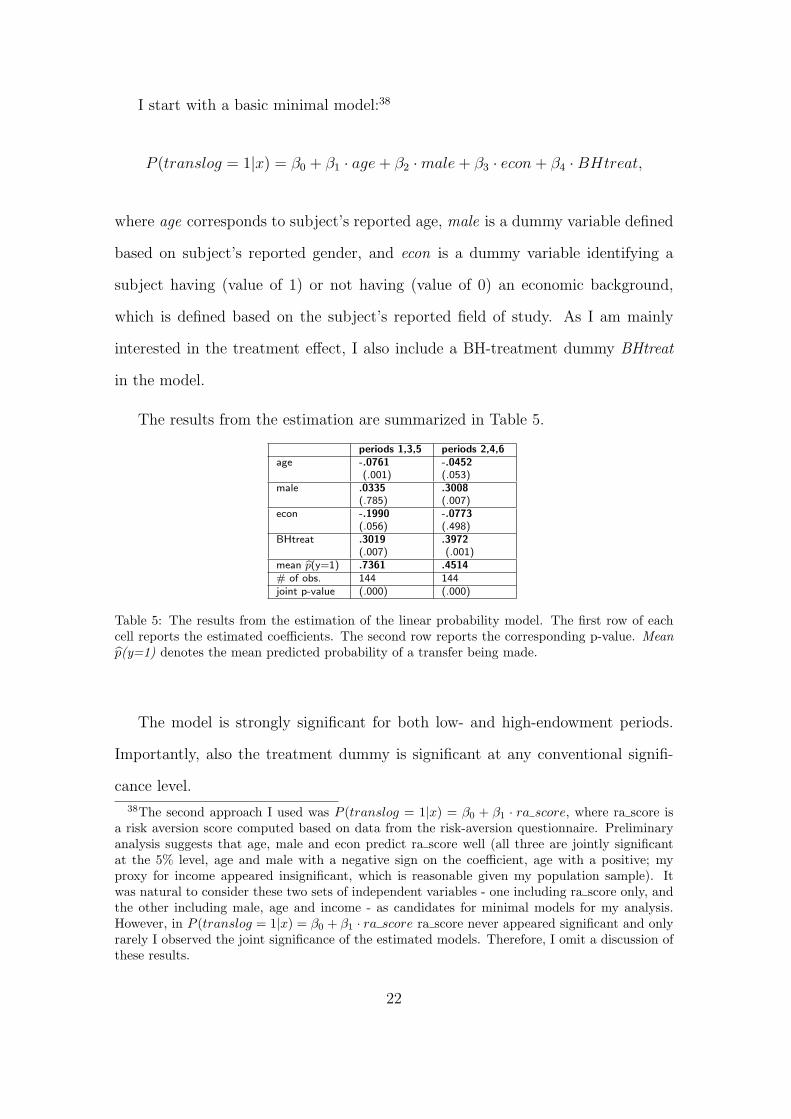
I start with a basic minimal model:38

P (translog = 1|x) = β0 + β1 · age + β2 · male + β3 · econ + β4 · BHtreat,

where age corresponds to subject’s reported age, male is a dummy variable defined

based on subject’s reported gender, and econ is a dummy variable identifying a

subject having (value of 1) or not having (value of 0) an economic background,

which is defined based on the subject’s reported field of study. As I am mainly

interested in the treatment effect, I also include a BH-treatment dummy BHtreat

in the model.

The results from the estimation are summarized in Table 5.

periods 1,3,5 periods 2,4,6age -.0761

(.001)-.0452(.053)

male .0335(.785)

.3008(.007)

econ -.1990(.056)

-.0773(.498)

BHtreat .3019(.007)

.3972(.001)

mean bp(y=1) .7361 .4514# of obs. 144 144joint p-value (.000) (.000)

Table 5: The results from the estimation of the linear probability model. The first row of eachcell reports the estimated coefficients. The second row reports the corresponding p-value. Meanp(y=1) denotes the mean predicted probability of a transfer being made.

The model is strongly significant for both low- and high-endowment periods.

Importantly, also the treatment dummy is significant at any conventional signifi-

cance level.

38The second approach I used was P (translog = 1|x) = β0 + β1 · ra score, where ra score isa risk aversion score computed based on data from the risk-aversion questionnaire. Preliminaryanalysis suggests that age, male and econ predict ra score well (all three are jointly significantat the 5% level, age and male with a negative sign on the coefficient, age with a positive; myproxy for income appeared insignificant, which is reasonable given my population sample). Itwas natural to consider these two sets of independent variables - one including ra score only, andthe other including male, age and income - as candidates for minimal models for my analysis.However, in P (translog = 1|x) = β0 + β1 · ra score ra score never appeared significant and onlyrarely I observed the joint significance of the estimated models. Therefore, I omit a discussion ofthese results.

22

The mean predicted probability of transfer in the low-endowment periods is

.7361 for the pooled sample. For the B treatment it is .5278, for the BH treatment

.9444. In the high-endowment periods, the mean predicted probability of transfer is

considerably lower. For the pooled sample it is .4514, for the B treatment .2222, and

for the BH treatment .6806. Thus, as I expected, the transfer rate is much higher

in the high-incentive treatment. For both treatments the transfer rate is higher

in low- than in high-endowment periods. This result contradicts the theoretical

prediction39 (we find the same result in the context treatment, see Krajcova &

Ortmann 2008).

Age is significant at the 5% level for low-endowment periods and at the 10% level

for high-endowment periods, in both cases with a negative sign on the coefficient.

An additional year of age reduces the probability of transfer by .08 with low and

by .05 with high endowment.

The male dummy is not significant for low-endowment periods, but I get strong

significance for high-endowment periods.40 In both cases, the sign on the coeffi-

cient is positive, meaning that men are more likely to transfer – by .03 when the

endowment is low and by .30 when it is high – than women.

Econ is significant at the 10% level for low endowment and not significant for

high endowment periods. The sign on the coefficient is, in both cases, negative.

Thus, subjects with an economic background are less likely to transfer.

The BHtreat dummy is significant at the 1% level for both low- and high-

endowment periods. The sign on the coefficient is positive meaning that, as I

39Recall that in the equilibrium Participant X always transfers with a high endowment andnever transfers with a low.

40I find no evidence of gender-specific effects such as in Krajcova & Ortmann (2008). In thefirst stage, both male and female participants transfer more in the BH treatment than in the Btreatment. I find some differences in the behavior of men and women – in the second stage withhigh endowment; and for sequential choices in the E2 node with both low and high endowment.In all three cases, however, the size of the female subsample is too small to make any plausibleinferences.

23

expected, subjects in the high-incentive treatment are more likely to transfer – by

.30 with low and by .40 with high endowment – than subjects in the benchmark

treatment.

In general, the main results that can be observed from the descriptive data are

also statistically significant.

5 Discussion

I expected that subjects in my experiment might not behave in complete accordance

with the theoretical predictions made under the assumption of rationality and risk-

neutrality. Apart from risk attitudes, phenomena such as altruism, reciprocity

(positive or negative) and/or trust might play important roles. In fact, in my data

I observe considerable deviations from equilibrium at some stages of the game.

The change in parameterization shifts some of the results closer and some further

away from the predictions. In this section, I discuss the results, and provide some

explanations for these deviations and for the observed treatment effect. I also derive

implications for experimental design and the implementation of the experimental

testing of leniency programs.

In the first stage, for both treatments, I observe higher transfer rates in low-

than in high-endowment periods, which contradicts the theoretical prediction.41 In

the BH treatment the fraction of out-of-equilibrium choices is even higher than in

the B treatment. A similar result is found for the context treatment in Krajcova

& Ortmann (2008).

I note that the theoretical prediction is computed under the assumption of risk

41Recall that in the equilibrium Participant X always transfers with a high endowment andnever transfers with a low. Or, in other words, given the leniency program currently in force,theoretically, with a low endowment (thus, a low bribe) an occasional illegal transaction is notimplementable.

24

neutrality, which, as also suggested by the data from the risk-aversion questionnaire,

is not likely to hold in my sample. My subjects appear to be modestly risk-averse,

in accordance with the typical finding in the experimental literature (e.g. Holt &

Laury 2002, Harrison, Johnson, McInnes & Rutstrom 2005). When I computed the

theoretical prediction for a (modestly) risk averse subject, I found that under some

(reasonable) assumptions, my chosen parameterization can lead to a no-corruption

equilibrium also for the high-endowment periods.42 That is, for risk-averse subjects,

it might in fact be optimal not to transfer a high endowment.

In addition, my subjects might exhibit the “preference for inclusion” reported

by Cooper & Van Huyck (2003). The authors find that subjects presented with

an extensive form game are significantly more likely to make choices that allow

their co-player to make a choice – and thereby to affect final payoffs – rather than

choosing a terminal node. In an extensive form game this “(non)inclusion” is more

salient. In my game, “inclusion” introduces a risk of significant loss. Together with

risk- or loss-avoidance, it might have resulted in subjects with a “preference for

inclusion” being willing to transfer and continue playing the game, but only being

ready to risk the low endowment and preferring to keep the high endowment for

sure.

Furthermore, note that the difference in expected payoffs to Participant Y from

42I assume a standard CRRA utility function u(x) = x(1−r). The average risk-aversion co-efficient in my sample is about 0.03; the maximal is about 0.1. As the bribery game involvesnodes with negative payoffs, some assumptions need to be made about the utility function inthe negative domain. Prospect theory suggests that in the negative domain, the steepness ofthe utility function might be about twice as much as in the positive domain. For illustration, Icomputed the theoretical prediction for a risk-neutral subject in the B treatment assuming two dif-ferent levels of (dis)utility from paying a 300 CZK penalty after detection: u(−300) = −u(450);and u(−300) = −u(600). For low endowment, the theoretical prediction is the same as for arisk-neutral subject. For high endowment it changes. For an extremely risk-averse participant(r = 0.1), the disutility of 450 still predicts a corruption equilibrium, however, the disutility of600 predicts a no-corruption equilibrium. For an average risk-aversion coefficient (r = 0.03), thedisutility of 450 is sufficient to change the theoretical prediction. I obtained analogical results forthe BH treatment (because of a different parameterization, the relevant disutilities for the BHtreatment are u(−200) = −u(300); and u(−200) = −u(400)).

25

choosing Denounce or Action a is relatively small43 in both treatments (assuming

that Participant X will react rationally), whereas the difference in payoffs to Partic-

ipant X is substantial. Therefore, an altruistic Participant Y might prefer choosing

Action a even in low-endowment periods, when this action is not maximizing the

expected payoff. Or, alternatively, choosing Action a might be an act of positive

reciprocity. In low-endowment periods, a rational Participant X might expect a

rational Participant Y to choose Denounce and therefore he would not transfer. A

Participant X who is trusting might expect Participant Y to choose Action a in the

second stage and therefore he might want to transfer.

In the BH treatment, the difference in expected payoffs to Participant Y is about

the same, but the possible gain to Participant X (after Action a has been chosen)

is considerably larger than in the B treatment. That is why, if the above arguments

hold, the new paramererization might shift the choices even further away from the

equilibrium. This is indeed what I observe in the data.

In the second stage, for both treatments, I observe about an equal split between

choosing Denounce and Action a, for both low- and high-endowment periods. Noth-

ing is almost never chosen.

Payoffs for Participant Y resulting from Nothing and Action a are the same,

but taking into account the likely decisions of Participant X in the following stage,

he is more likely to collect a higher payoff after he chooses Action a. This seems to

be correctly recognized by the vast majority of my subjects.

As regards the relative indecisiveness of subjects between choosing Denounce

or Action a, I repeat the arguments mentioned above – the difference in expected

payoffs is relatively small, which together with different preferences for altruism

and reciprocity might have produced these results.

43Note that this results from the nature of the game (see Figure 1).

26

In the E1 node, a new parameterization shifts the results closer to the prediction.

Intuitively, if subjects exhibit negative reciprocity, this becomes the more salient

the more there is at stake.

In the E2 node, the majority of subjects plays equilibrium in both treatments. In

the BH treatment the fraction of subjects who play equilibrium is slightly smaller.

It is still the majority, though.

Altogether, my data to some extent confirm the main result of Buccirossi &

Spagnolo (2006) – an occasional illegal transaction is implementable when a leniency

policy is in place. This becomes especially visible in the high-incentive treatment

with high endowment. I observe a sensitive reaction to a parametric change that

does not affect the theoretical prediction. My finding suggests that calibration, i.e.

parameterization that reflects “real-life” situations reasonably well, might even be

more important than in other scenarios. My data, in addition, suggest that other

factors might be important as well. Trust and preferences towards others might

play an important role. Further experimental testing of leniency policies might

have to take these findings into account.

27

References

Abbink, K., Hennig Schmidt, H., (2006). Neutral versus Loaded Instructions in a

Bribery Experiment, Experimental Economics 9(2), 103-121.

Abbink, K., Irlenbusch, B., Renner, E., (2002). An Experimental Bribery Game,

Journal of Law, Economics, and Organization 18(2), 428-454.

Apesteguia, J., Dufwenberg, M., Selten, R., (2007). Blowing the Whistle. Economic

Theory 31, 143–166.

Bigoni, M., Fridolfsson, S.-O., Le Coq, C., Spagnolo , G., (2007). Fines, Leniency,

Rewards and Organized Crime: Evidence from Antitrust Experiments. [manuscript

dated November 15, 2007, not for distribution]

Bigoni, M., Fridolfsson, S.-O., Le Coq, C., Spagnolo, G., (2008). Risk Aversion,

Prospect Theory, and Strategic Risk in Law Enforcement: Evidence From an An-

titrust Experiment. [manuscript dated February 1, 2008, not for distribution]

Buccirossi, P., Spagnolo, G., (2006). Leniency Policies and Illegal Transactions, Jour-

nal of Public Economics 90, 1281–1297.

Cohen, J., (1988). Statistical Power for the Behavioral Sciences, 2nd edition. Lawrence

Erlbaum Associates Inc, Hillsdale.

Cooper, D., J., Van Huyck, J.,B., (2003). Evidence on the Equivalence of the Strategic

and Extensive Form Representation of Games, Journal of Economic Theory 110,

290-308.

Dusek, L., Ortmann, A., Lızal, L., (2005). Understanding Corruption and Corrupt-

ibility through Experiments. Prague Economic Papers 14, 147-162.

28

Fischbacher, U., (2007). Z-tree: Zurich Toolbox for Ready-made Economic Experi-

ments - Experimenter’s Manual. Experimental Economics 10(2), 171-178(8).

Gigerenzer, G., Hoffrage, U., (1995). How to Improve Bayesian Reasoning without

Instruction: Frequency Formats. Psychological Review 102, 684–704.

Goeree, J., K., Holt, C., A., (2001). Ten Little Treasures of Game Theory, and Ten

Intuitive Contradictions. American Economic Review 91, 1402-1422.

Gupta, S., Davoodi, H., Alonso-Terme, R., (2002). Does Corruption Affect Income

Inequality and Poverty? Economics of Governance 3(1), 23-45.

Harrison, G., W., Johnson, E., McInnes, M., Rutstrom, E., (2005). Risk Aversion and

Incentive Effects: Comment. American Economic Review 95 (3), 897-901.

Hertwig, R., Ortmann, A., (2004). The Cognitive Illusions Controversy: A Method-

ological Debate in Disguise That Matters to Economists. in Zwick, R., Rapoport,

A. (eds.), Experimental Business Research, Kluwer Academic Publishers, Boston,

MA, 361- 378.

Holt, C., A., Laury, S., K., (2002). Risk Aversion and Incentive Effects, The American

Economic Review 92 (5), 1644-1655.

Hwang, J., (2002). A Note on the Relationship Between Corruption and Government

Revenue. Journal of Economic Development 27(2), 161-178.

Kamecke, U., (1997). Rotations: Matching Schemes that Efficiently Preserve the Best

Reply Structure of a One Shot Game, International Journal of Game Theory 26

(3), 409-417.

Krajcova, J., Ortmann, A., (2008). Testing Leniency Programs Experimentally: The

29

Impact of Natural Framing, CERGE-EI Working Paper Series, forthcoming.

Mauro, P., (1995). Corruption and Growth. Quarterly Journal of Economics, 110,

681-712.

Ortmann, A., Lızal, L., (2003). Designing and Testing Incentive-compatible and Effec-

tive Anti-corruption Measures, grant proposal successfully submitted to the Grant

Agency of the Czech Republic. Grant No. 402/04/0167.

Richmanova, J., (2006). In Search of Microeconomic Models of Anti-Corruption Mea-

sures – A Review, CERGE-EI Discussion Paper No. 2006-157.

Richmanova, J., Ortmann, A., (2008). A Generalization of the Buccirossi & Spagnolo

(2006) Model. CERGE-EI Discussion Paper No. 2008-194.

Roth, A., (2002). The Economist as Engineer: Game Theory, Experimentation, and

Computation as Tools for Design Economics, Econometrica 70(4), 1341-1378.

Rydval, O., (2007). The Impact of Financial Incentives on Task Performance: The

Role of Cognitive Abilities and Intrinsic Motivation, PhD dissertation, CERGE-EI.

Spagnolo, G., (2004). Divide et Impera: Optimal Leniency Programs, C.E.P.R. Dis-

cussion Paper No. 4840.

Tanzi, V., (1998). Corruption Around the World: Causes, Consequences, Scope and

Cures. IMF Working Paper 98/63.

Williamson, O., (1983). Credible Commitments: Using Hostages to Support Ex-

change. American Economic Review 73, 519-540.

30

APPENDIX 1

Comparing the data from periods before and after the switch of roles.

In Figure 4, I present the data from the before- and after-the-switch-of-roles

periods (before-switch data in the upper rows and after-switch data below) from

low- and high-endowment periods of the B treatment.

In both cases, I observe a somewhat higher transfer rate in the second six

periods. The transfer rate is higher in the low-endowment periods than in the high

before and after the switch of roles. In the B0 node, more subjects chose the safe

option (with no possibility of loss) after the switch of roles. In the E2 node, results

from before- and after-switch data are very similar, which is not the case of the E1

node, where the relative percentages shifted closer to the equilibrium prediction.

Figure 4: Before- vs. after-the-switch-of-roles data in the B treatment. Before-switch data are inthe upper rows and after-switch data are below.

In Figure 5, I present the data from before- and after-switch-of-roles periods

(before-switch data in the upper row and after-switch data below) from low- and

high-endowment periods of the BH treatment.

31

Figure 5: Before- vs. after-the-switch-of-roles data in the BH treatment. Before-switch data arein the upper rows and after-switch data are below.

In both cases, I observe no differences in the transfer rates after the switch of

roles. Similarly as in the first part, the transfer rate is higher in the low-endowment

periods than in the high after roles are switched. In the B0 node, less subjects chose

the safe option (with no possibility of loss) after the switch of roles in both low-

and high-endowment periods. In the E1 and E2 nodes, results form before- and

after-switch data are very similar. This is somewhat different evidence than that

from the B treatment.

32

APPENDIX 2

Robustness checks

I performed two types of robustness check of my estimation results. The first

regards the way I treated individual observations over rounds when running regres-

sions – this is discussed in the subsection Handling of the data. The second regards

the experimental design – I run several sessions of alternative treatments in which

I introduce only minor changes that do not appear to significantly affect behavior

of subjects – this is discussed in the subsection Pooling the sessions.

A. Handling of the data

Throughout the analysis I have defined three alternative dependent variables,

each of which captures slightly different information about the first-stage data.

Translog is a 0/1 dummy variable identifying transfer being made (value of 1)

or not (value of 0) in a particular period.

Atranslog is the average value of translog for one individual over periods 1, 3,

and 5 ( low-endowment periods) or 2, 4, and 6 (high-endowment periods).

Ltranslog defines the dominant choice of a subject in periods 1, 3, and 5 or 2, 4,

and 6. For a subject who has chosen Pay two or three times out of a total three

periods of interest, the dominant choice is 1; for a subject who has chosen Not Pay

two or three times out of total three periods of interest, the dominant choice is 0.

Then, using one of the three types of dependent variable, I conducted four

different types of regression analysis.

Clustered regressions – as discussed in the main text, I run a clustered (robust)44

linear probability model estimation with the binary variable translog as a dependent

variable.

44Standard errors are corrected for heteroskedasticity and for within-subject correlation.

33

Regressions on Averaged data – in this case, I run an ordinary least squares esti-

mation of atranslog. I analyze only averaged data, where higher values of atranslog

correspond to more transfers being made and thus to a stronger preference for this

choice.45

Regressions on the 1st or 2nd period data – I estimate LPM only on the 1st and

2nd period translog (for low- and high-endowment periods, respectively). In this

approach I am omitting part of the information, however I only use the part of the

data that is not affected by the experience from previous rounds.46

Regressions on Dominant Choice – I estimate LPM using ltranslog as a depen-

dent variable. Thus in this case, I am only looking at the dominant choice of each

subject.

First I look at effect size measures, whether they give robust results for all four

approaches to the data. The results are summarized in Table 6 below.

B BH effect sizeData mean std.dev. mean std.dev. odds ratio Cohen’s d

1,3,5 1st-period .583 .5036 .917 .2823 1.730 .8179average .528 .4495 .944 .2123 1.788 1.1827dominant .5 .5108 .958 .2041 1.916 1.1772all periods .528 .5027 .944 .2306 1.788 1.0629

2,4,6 2nd-period .292 .4643 .708 .4643 2.425 1.1118average .222 .3764 .681 .3330 3.068 1.2924dominant .25 .4423 .708 .4643 2.832 1.0107all periods .222 .4187 .681 .4695 3.068 1.0309

Table 6: Effect-size indices.

In all cases, the effects are large (recall that Cohen 1998 defines effect sizes of

d = 0.8 as large). The directions of the effects are the same in all cases – transferring

is higher in the high-incentive (BH) treatment.

Tables 7 and 8 below summarize the main results from the estimation for low-

45I also run poisson regressions on a count variable (counting the number of transfers made byan individual in the relevant three periods). The qualitative results are the same as with OLSand atranslog.

46I realize that for 2nd period data this may not be completely true if subjects fail to realizethat it is a different game they are playing in the high-endowment periods.

34

and high-endowment periods, respectively.

Periods 1,3,5clustered averaged 1st-period dominant

age -.0761(.001)

-.0761(.002)

-.0751(.023)

-.0720(.006)

male .0335(.785)

.0335(.791)

.1024(.465)

.0526(706)

econ -.1990(.056)

-.1990(.064)

-.1349(.298)

-.2221(.079)

BHtreat .3019(.007)

.3019(.009)

.2453(.072)

.3334(.014)

const 2.3445(.000)

2.3445(.000)

2.2788(.004)

2.2284(.001)

mean bp(y=1) .7361 .7361 .75 .7292# of obs. 144 48 48 48joint p-value .000 .000 .006 .000

Table 7: Results from clustered regressions vs. regressions on averaged, 1st-period, and dominant-choice data from low-endowment periods.

Periods 2,4,6clustered averaged 2nd-

perioddominant

age -.0452(.053)

-.0452(.061)

-.0454(.166)

-.0449(.158)

male .3008(.007)

.3008(.009)

.1888(.243)

.3011(.044)

econ -.0773(.498)

-.0773(.511)

-.2425(.138)

-.0448(.785)

BHtreat .3972(.001)

.3972(.002)

.2844(.083)

.4122(.015)

const 1.0597(.046)

1.0597(.046)

1.3414(.067)

1.0561(.139)

mean bp(y=1) .4514 .4514 .5 .4792# of obs. 144 48 48 48joint p-value .000 .000 .003 .000

Table 8: Results from clustered regressions vs. regressions on averaged, 1st-period, and dominant-choice data from high-endowment periods.

Under all four approaches, the treatment effect is robust – I find the treatment

dummy BHtreat significant. Except for the 1st- and 2nd-period data, it is significant

at the 5% level. The sign on the coefficient is positive in all cases and for both

low- and high-endowment periods, meaning that the transfer rate is higher in the

high-incentive treatment.

As regards other explanatory variables, the results for low-endowment periods

are very similar to results from clustered regressions – age is significant at 5%, male

35

is not significant, and econ is significant only at the 10% level and not significant

for the 1st-period data.

For high-endowment periods, the the results are not as robust. Age is significant

at the 10% level for clustered and averaged data, and not significant for the 2nd-

period and dominant-choice data. Male is significant at the 5% level with the

exception of the 2nd-period data where it is not significant. Econ is never significant.

The results suggest that there is larger variation in high-endowment data, which

is more difficult to explain by the explanatory variables. I believe that a larger

sample size would lead to more robust results.

As regards sizes and signs of coefficients, the results are very robust, especially

for clustered, averaged and dominant choice data.

B. Pooling the sessions

In addition to the benchmark treatment B and to the high-incentive treatment

BH, I conducted two plus two sessions of “automatic” treatments A and AI. Under

both treatments, A and AI, I used the same game and same parameterization

as in the B treatment. The only difference was that in automatic treatments,

each subject played against a computer program, with six subjects in the role of

Participant X and six subjects in the role of Participant Y. The computer program

always played a (subgame perfect) optimal strategy. Subjects were acquainted with

these facts in the instructions.

The only difference between the A and AI treatments was that in the AI subjects

received, as a separate part of the instructions, a so-called Backwards Induction

Tutorial, intended to explain the basic principles of using backwards induction.

Before pooling the data from different treatments I performed basic statistical

tests in order to discover significant differences in the distributions of choices –

Fisher’s Exact test and Wilcoxon rank-sum test. I find no evidence of significant

36

differences in the distributions of choices between the A, AI and B treatments.

Afterwards, I performed two types of pooled analysis: 1) pooling the data from

the A and B treatments vs. the BH treatment and 2) pooling the data from the

A, AI and B treatments vs. the BH treatment. My main result, the significance of

treatment dummy at 5%, remains unaffected.

See Table 9 for the regression results for low- and high-endowment periods.

Clearly, pooling slightly different treatments leads to noisier results, which is not

very surprising. Importantly, the treatment dummy remains significant at the 5%

level.

Periods 1,3,5 Periods 2,4,6B vs. BH B,A vs. BH B,A,AI vs. BH B vs. BH B,A vs. BH B,A,AI vs. BH

age -.0761(.001)

-.0652(.007)

-.0376(.160)

-.0452(.053)

-.0229(.338)

-.0186(.418)

male .0335(.785)

-.0097(.932)

-.0178(.863)

.3008(.007)

.1726(.128)

.1079(.317)

econ -.1990(.056)

-.2152(.026)

-.1572(.117)

-.0773(.498)

-.1638(.127)

-.1365(.164)

BHtreat .3019(.007)

.2898(.001)

.3550(.000)

.3972(.001)

.2949(.007)

.2831(.006)

const 2.3445(.000)

2.1577(.000)

1.4756(.016)

1.0597(.046)

.7994(.133)

.7613(.130)

mean bp(y=1) .7361 .7111 .6806 .4514 .4556 .4491# of obs. 144 180 216 144 180 216joint p-value .000 .000 .000 .000 .000 .002

Table 9: Results from the estimation of basic vs. extended data sets.

37

Individual researchers, as well as the on-line and printed versions of the CERGE-EI Working Papers (including their dissemination) were supported from the following institutional grants:

• Center of Advanced Political Economy Research [Centrum pro pokročilá politicko-ekonomická studia], No. LC542, (2005-2009),

• Economic Aspects of EU and EMU Entry [Ekonomické aspekty vstupu do Evropské unie a Evropské měnové unie], No. AVOZ70850503, (2005-2010);

• Economic Impact of European Integration on the Czech Republic [Ekonomické dopady evropské integrace na ČR], No. MSM0021620846, (2005-2011);

Specific research support and/or other grants the researchers/publications benefited from are acknowledged at the beginning of the Paper. (c) Jana Krajčová, 2008 All rights reserved. No part of this publication may be reproduced, stored in a retrieval system or transmitted in any form or by any means, electronic, mechanical or photocopying, recording, or otherwise without the prior permission of the publisher. Published by Charles University in Prague, Center for Economic Research and Graduate Education (CERGE) and Economics Institute ASCR, v. v. i. (EI) CERGE-EI, Politických vězňů 7, 111 21 Prague 1, tel.: +420 224 005 153, Czech Republic. Printed by CERGE-EI, Prague Subscription: CERGE-EI homepage: http://www.cerge-ei.cz Editors: Directors of CERGE and EI Managing editors: Deputy Directors for Research of CERGE and EI ISSN 1211-3298 ISBN 978-80-7343-170-9 (Univerzita Karlova. Centrum pro ekonomický výzkum a doktorské studium) ISBN 978-80-7344-159-3 (Národohospodářský ústav AV ČR, v. v. i.)