J. Fluid Mech. (2013), . 737, pp. doi:10.1017/jfm.2013.560

J. Fluid Mech. (2013), vol. 737, pp. 78–104. c© Cambridge University Press 2013 78doi:10.1017/jfm.2013.560

Optimal vortex formation in a self-propelledvehicle

Robert W. Whittlesey1 and John O. Dabiri1,2,†1Graduate Aeronautical Laboratories, California Institute of Technology Pasadena, CA 91125, USA

2Bioengineering, California Institute of Technology Pasadena, CA 91125, USA

(Received 6 June 2013; revised 16 September 2013; accepted 16 October 2013;first published online 15 November 2013)

Previous studies have shown that the formation of coherent vortex rings in the near-wake of a self-propelled vehicle can increase propulsive efficiency compared with asteady jet wake. The present study utilizes a self-propelled vehicle to explore thedependence of propulsive efficiency on the vortex ring characteristics. The maximumpropulsive efficiency was observed to occur when vortex rings were formed of thelargest physical size, just before the leading vortex ring would pinch off from itstrailing jet. These experiments demonstrate the importance of vortex ring pinch off inself-propelled vehicles, where coflow modifies the vortex dynamics.

Key words: biological fluid dynamics, propulsion, vortex dynamics

1. IntroductionThe presence of coherent vortical structures in the near-wake of a jet, hereafter

referred to as ‘vortex-enhanced propulsion’, has been studied extensively andshown to increase propulsive performance in self-propelled vehicles (Siekmann 1962;Weihs 1977; Muller et al. 2000a; Krueger 2001; Krueger & Gharib 2003, 2005;Finley & Mohseni 2004; Choutapalli 2007; Bartol et al. 2008; Krieg & Mohseni2008, 2010, 2013; Moslemi 2010; Moslemi & Krueger 2010, 2011; Ruiz, Whittlesey& Dabiri 2011). Weihs (1977), using many assumptions, analytically predicted anincrease of 50 % in the average thrust through the use of vortex-enhanced propulsion.Later experimental work by Krueger & Gharib (2005) measured increases of up to90 % of the propulsive thrust by optimization of the vortex ring characteristics. Ruizet al. (2011) extended the results from stationary nozzles to a self-propelled vehicle,showing that vortex-enhanced propulsion can yield up to a 50 % increase in thepropulsive efficiency over a steady jet.

The vortices formed during vortex-enhanced propulsion can be characterized usingthe vortex formation time, tGRS , defined as

tGRS ≡ L

D0= Uptp

D0, (1.1)

where L is the length of a fluid slug ejected from the nozzle, D0 is the nozzle diameter,Up is the average piston velocity and tp is the discharge time, as defined in Gharib,

† Email address for correspondence: [email protected]

mailto:[email protected]

Optimal vortex formation in a self-propelled vehicle 79

Rambod & Shariff (1998). This definition is based on the use of a piston–cylinderapparatus for producing vortex rings in a quiescent tank. The hat on tGRS denotes anon-dimensional quantity. The formation time, tGRS , can be thought of physically asthe non-dimensional piston travel distance (L) or alternatively as the non-dimensionalpulse duration (tp). Gharib et al. (1998) demonstrated that vortex ring pinch off, aphenomenon where a forming vortex ring is kinematically separated from its trailingjet, occurs at a critical formation time tGRS ≈ 4. Krueger & Gharib (2003) showedthat for isolated vortex rings the pulse-averaged thrust normalized by the momentumflux is maximized at this critical formation time, known as the formation number F.Krueger, Dabiri & Gharib (2003, 2006) further showed that the formation number, F,can be reduced from its typical value of 4 when in the presence of coflow, such as thatoccurring in a self-propelled vehicle.

Ruiz et al. (2011) achieved significant increases in propulsive efficiency usingvortex-enhanced propulsion, but did not explore the dependence of propulsiveefficiency on vortex formation time. Moslemi & Krueger (2010, 2011) and Nichols& Krueger (2012) explored a range of formation time for their self-propelled vehicle,however only for relatively low Reynolds numbers (2 × 102–2 × 104, based on thevehicle length). The present work explores a range of vortex ring formation timesat higher Reynolds number, relevant to larger autonomous and manned underwatervehicle propulsion, to better understand the dependence of propulsive efficiency onvortex ring formation.

The self-propelled vehicle used in these experiments utilized self-excited oscillationsof a collapsible tube under external pressure to generate vortex rings. By varyingthe flow rate and external pressure, a wide range of vortex ring formation timesencompassing the threshold for vortex ring pinch off could be studied. The vehicleoperated in the Reynolds number range of Re = 9 × 104–1 × 106, based on vehiclelength. The wake of the vehicle was characterized using laser Doppler velocimetry(LDV) and dye visualization in order to quantify propulsive efficiency and wake vortexdynamics.

This paper is organized as follows. Section 2 describes the self-propelled vehicleand mechanism for generating vortices in its near-wake. The results of the experimentsare presented in § 3, with a particular emphasis on the vortex ring formationcharacteristics and their effect on the measured vehicle efficiency. Finally, § 4 discussesthe results.

2. Methods2.1. Passive vortex generator design and vehicle integration

2.1.1. Main vehicleFor the self-propelled tests, a passive vortex generator (PVG) was designed and

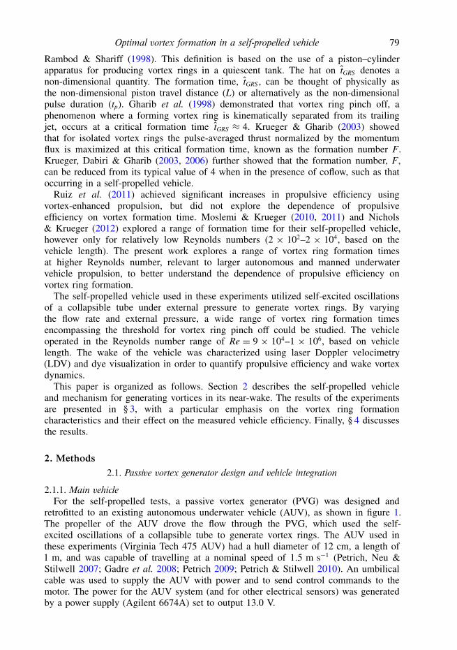
retrofitted to an existing autonomous underwater vehicle (AUV), as shown in figure 1.The propeller of the AUV drove the flow through the PVG, which used the self-excited oscillations of a collapsible tube to generate vortex rings. The AUV used inthese experiments (Virginia Tech 475 AUV) had a hull diameter of 12 cm, a length of1 m, and was capable of travelling at a nominal speed of 1.5 m s−1 (Petrich, Neu &Stilwell 2007; Gadre et al. 2008; Petrich 2009; Petrich & Stilwell 2010). An umbilicalcable was used to supply the AUV with power and to send control commands to themotor. The power for the AUV system (and for other electrical sensors) was generatedby a power supply (Agilent 6674A) set to output 13.0 V.

80 R. W. Whittlesey and J. O. Dabiri

PVG cut-away Highlighted media

143 cm

12 c

m

Direction of travel

A

A

PVG cut-away

Exterior

Highlighted media

(a)

(b)

FIGURE 1. Schematic drawings of PVG-integrated AUV. (a) Side view of the PVG-integrated AUV. The top figure shows the complete system exterior with the centre figureshowing the system with a cut plane parallel to the page through the middle of the PVG. Thecolours highlight the different components making up the assembly: blue is the AUV, red isthe PVG internal frame, green is the PVG cover and white denotes the collapsible tube. Thebottom figure highlights the different media within the device: blue is water, yellow is air andblack is solid material. The section line, AA, in the top figure corresponds to the section viewin (b). (b) Section view of the integrated PVG system (section line AA in a). The colouringin the left figure highlights the different components making up the assembly of the PVG andthe right figure highlights the different media, as in (a).

The AUV components used in these experiments were based on standard remote-control hobby parts. A servo controller (Pololu Micro Maestro) was connected tothe controlling computer. The servo controller commanded a motor speed controller(Hyperion Titan 20A Hi-Pro) attached to the AUV propeller motor (Hyperion ZS2209-30). This motor was geared down in a 40:19 ratio to the propeller shaft. The input tothe motor, called the ‘throttle setting’ and hereafter denoted by T , was related to thepulse width for a servo control which was translated by the motor controller into athree-phase, pulse-width-modulated (PWM) signal for driving the motor. The throttlesetting, T , ranged from 1000 (off) to 2000 (full throttle), with 1100 being the onsetof motor rotation. The throttle setting values are related to the power delivered to theAUV motor.

The selection and optimal axial location of the propeller was determined iteratively.A variety of propellers were tested with varying pitch, diameter, and blade number.Maximal thrust was produced by a three-bladed, 47 mm diameter propeller with apitch of 1.4 constructed of fibreglass-reinforced plastic. The propeller was mounted asfar aft as possible without striking the sides of the PVG contraction (cf. figure 1).

2.1.2. Integrated PVG designThe PVG is composed of an elastic tube conveying fluid encased in an airtight box,

schematically represented in figure 2. At certain values of the chamber pressure, Pe,


Pe

P1D0 P2

L0

FIGURE 2. Schematic of a PVG. Flow enters the inlet from the right and exits into ambientfluid through the nozzle on the left. The collapsible tube is denoted in the dotted line andhas length L0 and diameter D0. The pressure in the chamber is Pe, with the upstream anddownstream pressures relative to the collapsible tube denoted by P1 and P2, respectively.

and flow rate through the tube, self-excited oscillations can be sustained whichgenerate periodic pulses through the outlet (see Conrad 1969; Bertram 2003; Heil& Jensen 2003 and references therein). The pulses create vortex rings in the near-wakewhich enable a vehicle to use vortex-enhanced propulsion.

The design of the PVG upstream of the collapsible nozzle was adapted from thevehicle developed by Ruiz et al. (2011). The PVG-integrated AUV design is shown infigure 1(a). The PVG had a nozzle and tube diameter, D0, of 4 cm and a collapsibletube length, L0, of 16 cm. The wall thickness of the collapsible tube was 0.5 mm. Thetube was constructed out of sheets of silicone with a Shore A durometer hardness of35. The constructed tube had a glued seam, with an overlap of approximately 5 mm.The outer diameter of the PVG matched the diameter of the main vehicle to maximizethe internal air chamber volume while minimizing form drag. In addition, the PVGadded over 40 cm of length to the vehicle, making the total vehicle length 143 cm.The two-piece PVG was manufactured using stereolithography. This method yielded asmooth surface finish to minimize friction drag.

In order to reliably and accurately determine the oscillation frequency of the jet,the PVG was instrumented with a pressure transducer to measure the static pressuredownstream of the collapsible tube (P2 in figure 2). This pressure transducer measuredthe static pressure within the tube relative to the chamber pressure, Pe (cf. figure 2).This pressure is hereafter referred to as the ‘transmural’ pressure, Pt = Pe − P2. Thepressure tap was located 2 cm downstream of the collapsible tube (one-half of thetube diameter). The pressure transducer was attached to an instrumentation amplifiercircuit and read by a data acquisition system (DAQ; figure 5, K). Because the pressuretransducer was only used to measure frequency spectra (which was mean-subtracted),the pressure transducer and amplifier were calibrated using a water manometer forchanges in pressure only. The DAQ system (National Instruments USB-6221) wasconnected to a computer (hereafter the DAQ computer) that accessed the DAQ systemvia the MATLAB (Mathworks) software program. The DAQ system was configuredto record the pressure transducer signals at 5 kHz for the duration of a self-propelledrun. This sampling rate was sufficiently high to capture the higher-order modes ofthe signal and to ensure that software-based post-filtering would remove noise withinthe signal. The highest frequencies recorded were noise in the 1–1.5 kHz range fromthe motor controller’s PWM circuitry, thus the indicated sampling frequency of 5 kHz


satisfactorily encompassed the frequencies present within the laboratory environment.The DAQ system also recorded the voltage and current entering into the AUV vehicle.The current was measured by the voltage drop across a 0.05 � shunt resistor.

Ballast weight was added to the air chamber of the PVG to make the PVGapproximately neutrally buoyant. The combination of the ballast weight and thepressure transducers yielded a PVG air chamber volume of 2600 ± 50 cm3. Forfilling and draining the air in the chamber, two solenoid valves were used. Onesolenoid valve connected the PVG air chamber to a high-pressure line regulated at75 kPa through a 0.25 mm diameter flow-control orifice and was used for fillingthe chamber, hereafter referred to as the fill solenoid valve. The other solenoidvalve exhausted the PVG air chamber to the ambient, hereafter referred to asthe exhaust solenoid valve. Both of these solenoid valves were controlled using ametal–oxide–semiconductor field-effect transistor (MOSFET)-based circuit that drovethe high-current, 13 V solenoid using a low-current, 5 V digital signal from the DAQboard.

As the fill and exhaust solenoid valves were Boolean and not proportional, it wasnot feasible to precisely control the pressure in the chamber either manually or witha controller. Thus, the duration of time that the fill solenoid valve was open, hereafterreferred to as the chamber fill time, τ , was used as an independent variable in thetests.

To observe the effect the chamber fill time, τ , has on the tube cross-sectional area,images of the tube along the axial direction were recorded at different values of τ . Asample of these images is shown in figure 3. Using these images, the area of the tubecross-sectional area was calculated and normalized by the area of the tube at τ = 0 sto obtain a non-dimensionalized area fraction, α, defined as

α ≡ A

A0, (2.1)

where A is the cross-sectional area of the tube and A0 is the initial cross-sectional areaof the tube (i.e. τ = 0). These results are plotted in figure 4.

As shown in figure 3, it was observed that the tube undergoes buckling andcollapse with a mode 3 azimuthal collapse. This is distinct from some earlierstudies on collapsible tubes which showed a mode 2 azimuthal collapse (Conrad1969; Kececioglu et al. 1981; Bertram & Nugent 2005; Bertram & Tscherry 2006;Bertram, Truong & Hall 2008). This is expected due to the relatively thin wall of thecollapsible tube and the relatively short length of the tube used presently (L0/D0 = 4)(Love 1944; Palermo & Flaud 1987; Heil 1996; Fung 1997). It should be noted thatthe images shown in figure 3 are from conditions with no flow. However, during theself-excited oscillations, the tube was observed to maintain the same azimuthal modenumber.

The mode 3 azimuthal collapse may contribute to a reduction in the sensitivity ofα to τ due to the relationship between the tube compliance and its azimuthal collapsemode. Dion et al. (1995) showed that as the azimuthal mode of the tube bucklingincreased (e.g. from 2 to 3), the compliance of the tube decreased. A decreasedcompliance would yield a smaller change in the tube cross-sectional area for the samepressure change, and thus contribute to a sensitivity reduction.

2.2. Test facility and cart systemExperiments using the PVG-integrated AUV were conducted in a 40 m long free-surface water tunnel, a section of which is depicted in figure 5. The self-propelled tests


(a) (b) (c)

(d) (e) ( f )

FIGURE 3. Axial view of tube collapse at different chamber fill times, τ , for the PVG withthe propeller stationary. The collapsible tube is lightly coloured in these images with the PVGin grey. Images are aligned such that gravity points down: (a) τ = 0 s; (b) τ = 4 s; (c) τ = 8 s;(d) τ = 12 s; (e) τ = 15 s; (f ) τ = 20 s.

0

0.2

0.4

0.6

0.8

1.0

0 5 10 15 20

FIGURE 4. Cross-sectional area fraction of the collapsible tube from the PVG versus thechamber fill time, τ .

were conducted in a stationary ambient fluid. The AUV directly mounted to the sliderof an air bearing (Nelson Air Corp, RAB6; figure 5, F) that restricted the motion ofthe AUV along the longitudinal direction of the test section to 10 cm of travel. The


B A

C

D

E F

GH

IJ

K

FIGURE 5. Schematic of a section of the facility used for the PVG-integrated AUVexperiments. Letters indicate the item as follows: A, main vehicle (AUV); B, PVG; C, LDVprobe for jet measurements; D, traverse for moving LDV probe; E, short-range laser distancesensor; F, air bearing carriage (slider in black); G, cart motor showing toothed belt andpulleys used to move cart; H, laser beam from long-range laser distance sensor; I, feedbackcontroller box which interfaces to cart computer; J, LDV processing engine which receivesback scattered light from LDV probe (C) and interfaces to DAQ computer; and K, DAQsystem which interfaces to the DAQ computer.

carriage of the air bearing was mounted to a motorized cart system that moved on railsextending along the length of the tunnel test section. A feedback controller (figure 5,I) controlled the cart motor (figure 5, G) which moved the cart along the rails throughthe use of a toothed belt that extended the length of the tunnel. A short-range laserdistance sensor (Micro-Epsilon, optoNCDT 1302; figure 5, E) rigidly mounted to thecart measured the distance to an optical target attached to the slider of the air bearing.The feedback controller measured the position of the AUV along the air bearingcarriage using the short-range laser distance sensor and commanded the cart motor tomove the cart such that the relative position of the AUV was kept at a reference value.In this way, the AUV was maintained within the 10 cm of air bearing travel whileself-propelled along the full length of the water tunnel.

A long-range laser distance sensor (Micro-Epsilon, optoNCDT 1182; figure 5, H)measured the position of the cart along the tunnel. The combined values of the short-and long-range distance sensors precisely measured the position of the vehicle alongthe tunnel. The value of the position was Kalman filtered and used to obtain theposition and velocity, U∞, of the vehicle during self-propelled runs. An independentcomputer (hereafter the cart computer) sent control signals to the cart’s feedbackcontroller and recorded the cart’s position and velocity. The cart computer was alsoresponsible for issuing commands to the motor controller in the AUV.

2.3. Procedure for self-propelled runsThe throttle setting, T , and the chamber fill time, τ , were selected for each self-propelled run of the AUV. At the start of each run, the air chamber of the PVGwas filled for the duration specified by τ . The self-propelled portion of the run wasthen initiated. After the self-propelled portion of the run was completed, the exhaustsolenoid opened to allow the air chamber pressure to recover to the ambient labpressure. The cart was then slowly towed to the starting position for the next run.After the cart reached its starting position, the system waited an additional 15 s to


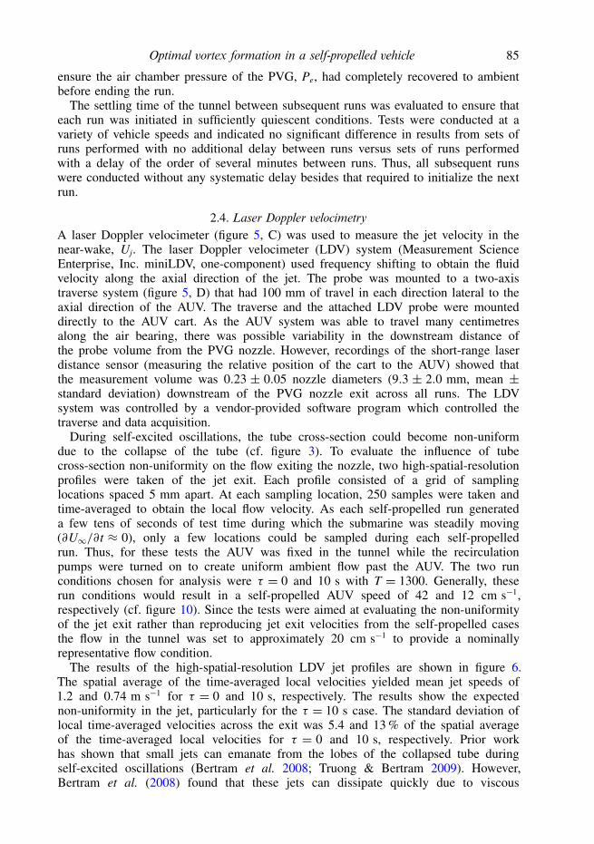
ensure the air chamber pressure of the PVG, Pe, had completely recovered to ambientbefore ending the run.

The settling time of the tunnel between subsequent runs was evaluated to ensure thateach run was initiated in sufficiently quiescent conditions. Tests were conducted at avariety of vehicle speeds and indicated no significant difference in results from sets ofruns performed with no additional delay between runs versus sets of runs performedwith a delay of the order of several minutes between runs. Thus, all subsequent runswere conducted without any systematic delay besides that required to initialize the nextrun.

2.4. Laser Doppler velocimetryA laser Doppler velocimeter (figure 5, C) was used to measure the jet velocity in thenear-wake, Uj. The laser Doppler velocimeter (LDV) system (Measurement ScienceEnterprise, Inc. miniLDV, one-component) used frequency shifting to obtain the fluidvelocity along the axial direction of the jet. The probe was mounted to a two-axistraverse system (figure 5, D) that had 100 mm of travel in each direction lateral to theaxial direction of the AUV. The traverse and the attached LDV probe were mounteddirectly to the AUV cart. As the AUV system was able to travel many centimetresalong the air bearing, there was possible variability in the downstream distance ofthe probe volume from the PVG nozzle. However, recordings of the short-range laserdistance sensor (measuring the relative position of the cart to the AUV) showed thatthe measurement volume was 0.23 ± 0.05 nozzle diameters (9.3 ± 2.0 mm, mean ±standard deviation) downstream of the PVG nozzle exit across all runs. The LDVsystem was controlled by a vendor-provided software program which controlled thetraverse and data acquisition.

During self-excited oscillations, the tube cross-section could become non-uniformdue to the collapse of the tube (cf. figure 3). To evaluate the influence of tubecross-section non-uniformity on the flow exiting the nozzle, two high-spatial-resolutionprofiles were taken of the jet exit. Each profile consisted of a grid of samplinglocations spaced 5 mm apart. At each sampling location, 250 samples were taken andtime-averaged to obtain the local flow velocity. As each self-propelled run generateda few tens of seconds of test time during which the submarine was steadily moving(∂U∞/∂t ≈ 0), only a few locations could be sampled during each self-propelledrun. Thus, for these tests the AUV was fixed in the tunnel while the recirculationpumps were turned on to create uniform ambient flow past the AUV. The two runconditions chosen for analysis were τ = 0 and 10 s with T = 1300. Generally, theserun conditions would result in a self-propelled AUV speed of 42 and 12 cm s−1,respectively (cf. figure 10). Since the tests were aimed at evaluating the non-uniformityof the jet exit rather than reproducing jet exit velocities from the self-propelled casesthe flow in the tunnel was set to approximately 20 cm s−1 to provide a nominallyrepresentative flow condition.

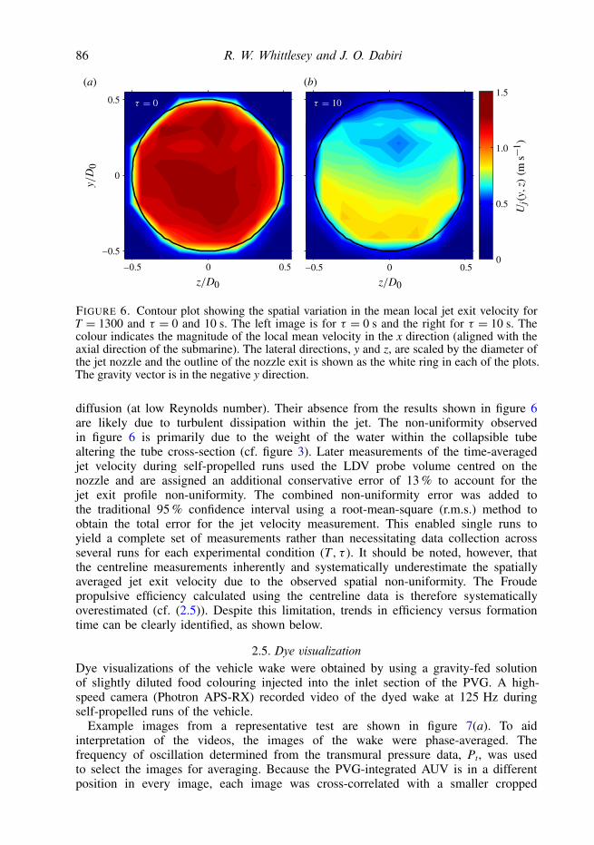
The results of the high-spatial-resolution LDV jet profiles are shown in figure 6.The spatial average of the time-averaged local velocities yielded mean jet speeds of1.2 and 0.74 m s−1 for τ = 0 and 10 s, respectively. The results show the expectednon-uniformity in the jet, particularly for the τ = 10 s case. The standard deviation oflocal time-averaged velocities across the exit was 5.4 and 13 % of the spatial averageof the time-averaged local velocities for τ = 0 and 10 s, respectively. Prior workhas shown that small jets can emanate from the lobes of the collapsed tube duringself-excited oscillations (Bertram et al. 2008; Truong & Bertram 2009). However,Bertram et al. (2008) found that these jets can dissipate quickly due to viscous


–0.5

0

0.5

–0.5 0 0.5 –0.5 0 0.50

0.5

1.0

1.5(a) (b)

FIGURE 6. Contour plot showing the spatial variation in the mean local jet exit velocity forT = 1300 and τ = 0 and 10 s. The left image is for τ = 0 s and the right for τ = 10 s. Thecolour indicates the magnitude of the local mean velocity in the x direction (aligned with theaxial direction of the submarine). The lateral directions, y and z, are scaled by the diameter ofthe jet nozzle and the outline of the nozzle exit is shown as the white ring in each of the plots.The gravity vector is in the negative y direction.

diffusion (at low Reynolds number). Their absence from the results shown in figure 6are likely due to turbulent dissipation within the jet. The non-uniformity observedin figure 6 is primarily due to the weight of the water within the collapsible tubealtering the tube cross-section (cf. figure 3). Later measurements of the time-averagedjet velocity during self-propelled runs used the LDV probe volume centred on thenozzle and are assigned an additional conservative error of 13 % to account for thejet exit profile non-uniformity. The combined non-uniformity error was added tothe traditional 95 % confidence interval using a root-mean-square (r.m.s.) method toobtain the total error for the jet velocity measurement. This enabled single runs toyield a complete set of measurements rather than necessitating data collection acrossseveral runs for each experimental condition (T, τ ). It should be noted, however, thatthe centreline measurements inherently and systematically underestimate the spatiallyaveraged jet exit velocity due to the observed spatial non-uniformity. The Froudepropulsive efficiency calculated using the centreline data is therefore systematicallyoverestimated (cf. (2.5)). Despite this limitation, trends in efficiency versus formationtime can be clearly identified, as shown below.

2.5. Dye visualizationDye visualizations of the vehicle wake were obtained by using a gravity-fed solutionof slightly diluted food colouring injected into the inlet section of the PVG. A high-speed camera (Photron APS-RX) recorded video of the dyed wake at 125 Hz duringself-propelled runs of the vehicle.

Example images from a representative test are shown in figure 7(a). To aidinterpretation of the videos, the images of the wake were phase-averaged. Thefrequency of oscillation determined from the transmural pressure data, Pt, was usedto select the images for averaging. Because the PVG-integrated AUV is in a differentposition in every image, each image was cross-correlated with a smaller cropped


(a)

(b)

(c)

FIGURE 7. Example results from dye visualizations of PVG wake. (a) Example raw imagesfrom dye-visualization run with T = 1700 and τ = 10. Each image is from approximately thesame phase of the oscillation cycle and are approximately 0.16 s apart. (b) Simulated stackingof dye visualization images from (a). (c) Final phase-averaged result including images from(a) after stacking (demonstrated in b) and image correction (brightness and contrast). Verticalbars in the wake are a processing artefact due to moving image boundaries relative to PVGnozzle (cf. b). The phase-averaged frame consists of six frames averaged together.

image of the aft-most portion of the PVG nozzle. This allowed for accurate trackingof the vehicle in each image. Images that were integer periods apart were stacked andaligned by their cross-correlated nozzle exit positions, as demonstrated in figure 7(b).The stacked images were then summed in their pixel intensity values and divided by


the number of images stacked. Because each image that was added to the overallphase-averaged image covered a different extent of the domain (e.g. one image showsmostly PVG and little of the wake whereas another image shows mostly wake andlittle of the PVG), different regions of the phase-averaged images have differentnumbers of phases averaged (e.g. all images show the wake near the vehicle whereasfewer images show the wake far from the vehicle). The differing domain extentgenerates a visual artefact that is visible in the resulting phase-averaged dye images asfaint vertical bars in the wake (see figure 7c).

2.6. Formation timeAs discussed previously, the formation time of the ejected fluid characterizes thevortex rings that are produced (cf. § 1). The standard definition of formation time, tGRS ,is given in (1.1). However, because the present system creates a train of vortex ringsfrom a moving system, two modifications to the formation time definition were made.

The first adjustment follows from Krueger et al. (2003, 2006), who considered thecreation of vortex rings created in coflow, where the ambient fluid is flowing paralleland in the same direction as the jetting fluid. They revised the formation time as

tKDG = tp(Up + Vc)

D0, (2.2)

where Vc is the average coflow velocity. This revised form of the formation timeis appropriate for the current study as the self-propelled vehicle experiences ambientcoflow in its frame of reference.

Because the ejection time tp ∼ 1/f , where f is the oscillation frequency, the secondadjustment was to redefine the formation time for self-propelled pulsed jets as

t = Uj + U∞fD0

, (2.3)

where Up and Vc have been replaced by Uj and U∞, respectively, to match thecurrent nomenclature. The oscillation frequency was calculated from the peak inthe fast-Fourier transform of the mean-subtracted transmural pressure, Pt, during thesteady-state portion of the self-propelled run. Furthermore, a threshold was applied tothe amplitude of the peak of the Fourier-transformed Pt such that only runs with peakamplitudes exceeding this threshold were considered oscillating cases.

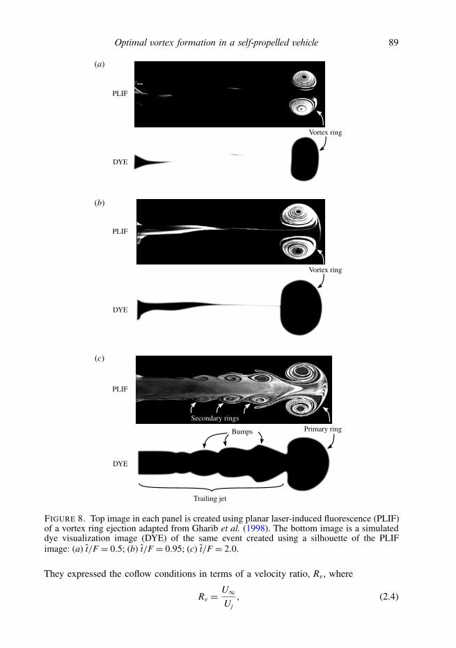
To assist in evaluating the existence of vortex ring pinch off, figure 8 shows boththe planar laser-induced fluorescence (PLIF) image of vortex ring ejection for threeformation times (from Gharib et al. 1998) and an illustrated silhouette depicting theexpected image of the same event using room lighting and dark dye, as in the currentexperiments. For figure 8(a,b) where the formation time is less than the formationnumber (t/F < 1), we expect to see the primary vortex ring along with a minimalamount of dye in its wake. In addition, as the formation number is increased, thesize of the vortex ring created increases as well. However, for fluid ejections that aregreater than the formation number (t/F > 1), as seen in figure 8(c), bumps along thetrailing jet form. These bumps correspond to secondary vortex rings that are createdafter the primary vortex ring has pinched off. The example in figure 8(c) is froma sufficiently high formation time (t/F = 2.0) that many secondary rings have beencreated in the trailing jet.

Krueger et al. (2006) measured the formation number, F, at which a vortex ringpinches off from its trailing jet and found that F is dependent on the coflow conditions.


Vortex ring

Vortex ring

Primary ring

Secondary rings

Trailing jet

Bumps

PLIF

DYE

PLIF

PLIF

DYE

DYE

(a)

(b)

(c)

FIGURE 8. Top image in each panel is created using planar laser-induced fluorescence (PLIF)of a vortex ring ejection adapted from Gharib et al. (1998). The bottom image is a simulateddye visualization image (DYE) of the same event created using a silhouette of the PLIFimage: (a) t/F = 0.5; (b) t/F = 0.95; (c) t/F = 2.0.

They expressed the coflow conditions in terms of a velocity ratio, Rv, where

Rv = U∞Uj, (2.4)


0.5

1.0

1.5

2.0

2.5

3.0

3.5

4.0

0.2 0.4 0.6 0.8

F

0

4.5

1.0

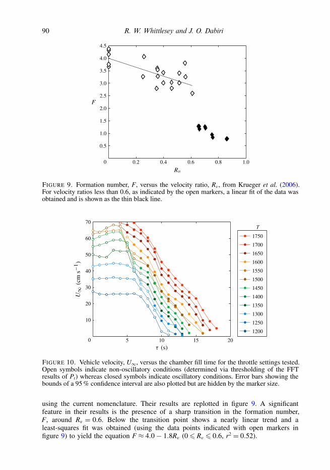
FIGURE 9. Formation number, F, versus the velocity ratio, Rv , from Krueger et al. (2006).For velocity ratios less than 0.6, as indicated by the open markers, a linear fit of the data wasobtained and is shown as the thin black line.

T

10

20

30

40

50

60

5 10 15

1750

1700

1650

1600

1550

1500

1450

1400

1350

1300

1250

1200

0

70

20

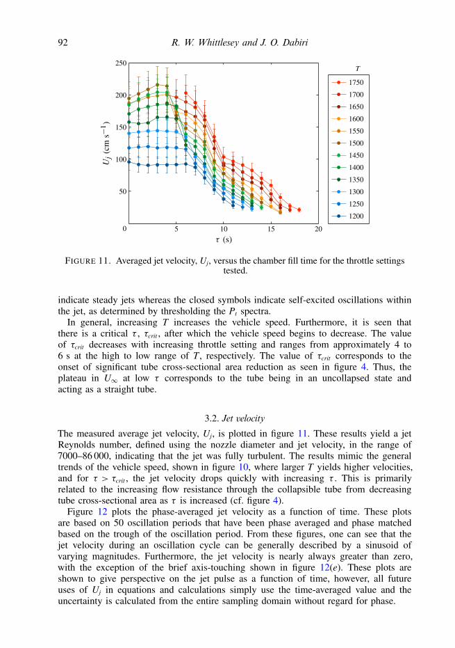
FIGURE 10. Vehicle velocity, U∞, versus the chamber fill time for the throttle settings tested.Open symbols indicate non-oscillatory conditions (determined via thresholding of the FFTresults of Pt) whereas closed symbols indicate oscillatory conditions. Error bars showing thebounds of a 95 % confidence interval are also plotted but are hidden by the marker size.

using the current nomenclature. Their results are replotted in figure 9. A significantfeature in their results is the presence of a sharp transition in the formation number,F, around Rv = 0.6. Below the transition point shows a nearly linear trend and aleast-squares fit was obtained (using the data points indicated with open markers infigure 9) to yield the equation F ≈ 4.0− 1.8Rv (0 6 Rv 6 0.6, r2 = 0.52).


2.7. EfficiencyThe propulsive efficiency of the vehicle was calculated using the Froude efficiency,defined as

η ≡ 2

1+ Uj

U∞

, (2.5)

where Uj is the time-averaged jet velocity and U∞ is the time-averaged speed of thevehicle (Prandtl 1952). Although this definition is derived under the assumption ofsteady flow, it is applied presently as it provides an objective performance metric andis commonly used in propulsion studies. The application of this definition to unsteadyflow conditions potentially constitutes a systematic error; therefore, its utility is limitedto comparison among unsteady flow cases rather than with equivalent steady flows.This caveat should be noted when comparing the quantitative results of this paper withother work.

The present measurements were conducted using a single-component LDV probe.Therefore, radial and azimuthal components of velocity are not included in theefficiency measurement. Because these components leave additional kinetic energyin the wake without contributing to thrust, their neglect leads to overestimation of theactual propulsive efficiency.

2.8. Error analysisFor measurements that yield a Gaussian distribution, error bounds can be obtainedthrough the use of Student’s t distribution to obtain a 95 % confidence interval forthe measurements (Beckwith, Marangoni & V, John 2007). For the jet velocity, Uj,the distribution of the sampled values is indeed Gaussian, even during oscillatingregimes, owing to the significant level of turbulence in the jet. As such, the errorbars for the mean jet velocity, Uj, are comprised of the 95 % confidence intervalusing Student’s t distribution in addition to 13 % of the mean value, where the latteraddition is due to the non-uniformity of the jet as observed in § 2.4. For any quantitythat is calculated based on measured values, the error is propagated by summing theproduct of the error in the measured value and the sensitivity of the calculated quantityto that measured value in a root-mean squared fashion (Beckwith et al. 2007). Todetermine the measurement uncertainty of the oscillation frequency, the measured Pt

during the steady portion of each run was divided into five equal time segments, andthe oscillation frequency of each segment was determined by applying a fast Fouriertransform (FFT) to the time-series data in each segment. The standard deviation of thefrequencies in each of the five segments was then tabulated for every run to determinethe measurement uncertainty of f , which was calculated to be nominally ±1.0 Hz.

3. Results3.1. Vehicle speed

The time-averaged vehicle speed, U∞, is plotted in figure 10 for various values of Tand τ . This yields a range of Re = 90 000–1 000 000 based on the vehicle length. ForT = 1600–1750, there is an absence of results for low chamber fill times because theseruns were not self-propelled, as the cart reached maximum speed which saturated thecontroller output. For each throttle setting tested, the chamber fill time was increaseduntil forward propulsion was no longer observed. The open symbols of figure 10


T

50

100

150

200

5 10 15 20

1750

1700

1650

1600

1550

1500

1450

1400

1350

1300

1250

1200

0

250

FIGURE 11. Averaged jet velocity, Uj, versus the chamber fill time for the throttle settingstested.

indicate steady jets whereas the closed symbols indicate self-excited oscillations withinthe jet, as determined by thresholding the Pt spectra.

In general, increasing T increases the vehicle speed. Furthermore, it is seen thatthere is a critical τ , τcrit , after which the vehicle speed begins to decrease. The valueof τcrit decreases with increasing throttle setting and ranges from approximately 4 to6 s at the high to low range of T , respectively. The value of τcrit corresponds to theonset of significant tube cross-sectional area reduction as seen in figure 4. Thus, theplateau in U∞ at low τ corresponds to the tube being in an uncollapsed state andacting as a straight tube.

3.2. Jet velocity

The measured average jet velocity, Uj, is plotted in figure 11. These results yield a jetReynolds number, defined using the nozzle diameter and jet velocity, in the range of7000–86 000, indicating that the jet was fully turbulent. The results mimic the generaltrends of the vehicle speed, shown in figure 10, where larger T yields higher velocities,and for τ > τcrit , the jet velocity drops quickly with increasing τ . This is primarilyrelated to the increasing flow resistance through the collapsible tube from decreasingtube cross-sectional area as τ is increased (cf. figure 4).

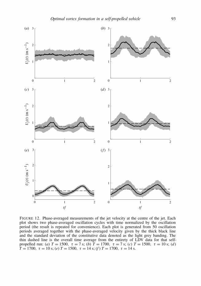
Figure 12 plots the phase-averaged jet velocity as a function of time. These plotsare based on 50 oscillation periods that have been phase averaged and phase matchedbased on the trough of the oscillation period. From these figures, one can see that thejet velocity during an oscillation cycle can be generally described by a sinusoid ofvarying magnitudes. Furthermore, the jet velocity is nearly always greater than zero,with the exception of the brief axis-touching shown in figure 12(e). These plots areshown to give perspective on the jet pulse as a function of time, however, all futureuses of Uj in equations and calculations simply use the time-averaged value and theuncertainty is calculated from the entire sampling domain without regard for phase.


1

2

1 20

3

1

2

1 20

3

1

2

1 20

3

1

2

20

3

1

2

1 2

tf

1

tf

0

0

3

1

2

1 20

3

(a) (b)

(c) (d)

(e) ( f )

FIGURE 12. Phase-averaged measurements of the jet velocity at the centre of the jet. Eachplot shows two phase-averaged oscillation cycles with time normalized by the oscillationperiod (the result is repeated for convenience). Each plot is generated from 50 oscillationperiods averaged together with the phase-averaged velocity given by the thick black lineand the standard deviation of the constitutive data denoted as the light grey banding. Thethin dashed line is the overall time average from the entirety of LDV data for that self-propelled run: (a) T = 1500, τ = 7 s; (b) T = 1700, τ = 7 s; (c) T = 1500, τ = 10 s; (d)T = 1700, τ = 10 s; (e) T = 1500, τ = 14 s; (f ) T = 1700, τ = 14 s.


T

6

8

10

12

0 5 10 15 20

1750

1700

1650

1600

1550

1500

1450

1400

1350

1300

12504

14

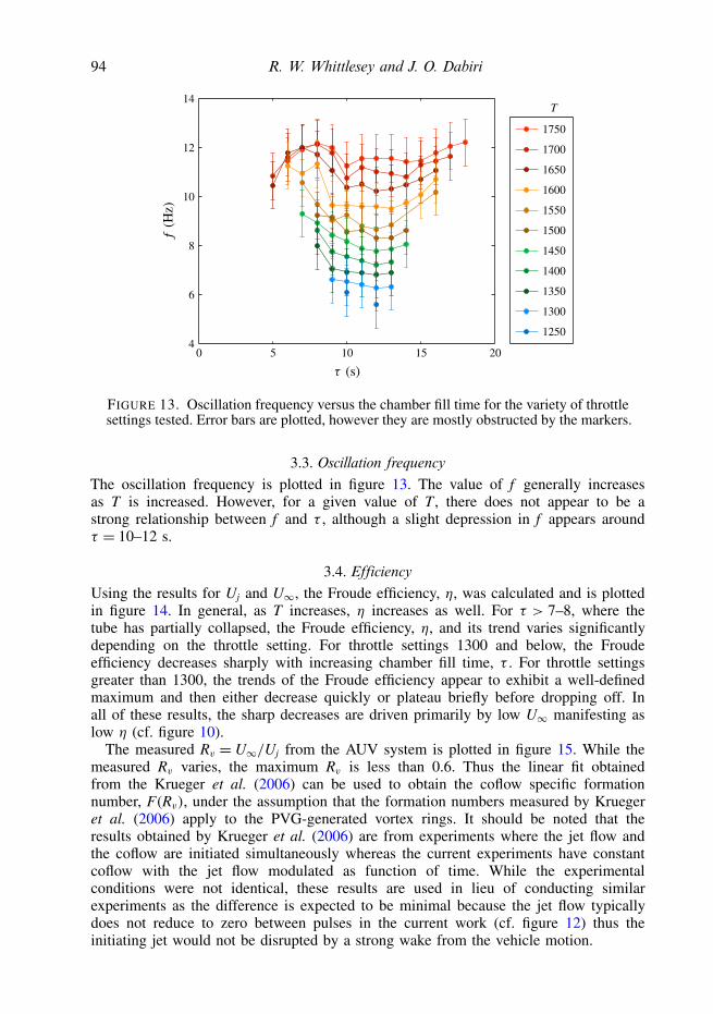
FIGURE 13. Oscillation frequency versus the chamber fill time for the variety of throttlesettings tested. Error bars are plotted, however they are mostly obstructed by the markers.

3.3. Oscillation frequencyThe oscillation frequency is plotted in figure 13. The value of f generally increasesas T is increased. However, for a given value of T , there does not appear to be astrong relationship between f and τ , although a slight depression in f appears aroundτ = 10–12 s.

3.4. EfficiencyUsing the results for Uj and U∞, the Froude efficiency, η, was calculated and is plottedin figure 14. In general, as T increases, η increases as well. For τ > 7–8, where thetube has partially collapsed, the Froude efficiency, η, and its trend varies significantlydepending on the throttle setting. For throttle settings 1300 and below, the Froudeefficiency decreases sharply with increasing chamber fill time, τ . For throttle settingsgreater than 1300, the trends of the Froude efficiency appear to exhibit a well-definedmaximum and then either decrease quickly or plateau briefly before dropping off. Inall of these results, the sharp decreases are driven primarily by low U∞ manifesting aslow η (cf. figure 10).

The measured Rv = U∞/Uj from the AUV system is plotted in figure 15. While themeasured Rv varies, the maximum Rv is less than 0.6. Thus the linear fit obtainedfrom the Krueger et al. (2006) can be used to obtain the coflow specific formationnumber, F(Rv), under the assumption that the formation numbers measured by Kruegeret al. (2006) apply to the PVG-generated vortex rings. It should be noted that theresults obtained by Krueger et al. (2006) are from experiments where the jet flow andthe coflow are initiated simultaneously whereas the current experiments have constantcoflow with the jet flow modulated as function of time. While the experimentalconditions were not identical, these results are used in lieu of conducting similarexperiments as the difference is expected to be minimal because the jet flow typicallydoes not reduce to zero between pulses in the current work (cf. figure 12) thus theinitiating jet would not be disrupted by a strong wake from the vehicle motion.


T

0

0.1

0.2

0.3

0.4

0.5

0.6

5 10 15

1750

1700

1650

1600

1550

1500

1450

1400

1350

1300

1250

1200

20

FIGURE 14. Froude efficiency, η, versus the chamber fill time for the throttle settings tested.Owing to excessive plot clutter, only a portion of the error bars have been plotted.

T

0

0.1

0.2

0.3

0.4

0.5

1 2 3 4 5 6 7

1750

1700

1650

1600

1550

1500

1450

1400

1350

1300

1250

FIGURE 15. Velocity ratio, Rv , versus the coflow formation time, t, for the throttle settingstested. Owing to excessive plot clutter, only a portion of the error bars have been plotted.

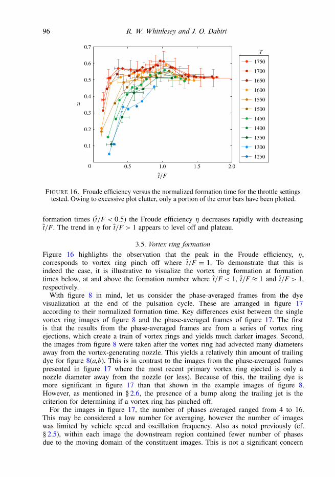
Equation (2.3) was used to calculate the formation time which was normalizedby the coflow specific formation number, F(Rv), to replot the efficiency values fromfigure 14. The normalized formation time plot is shown in figure 16. By plotting thedata in this way, the peaks that were previously spread out in figure 14 have becomealigned around t/F ≈ 1. Furthermore, the plot has flipped along the vertical directionas low values of η are correlated with low values of t/F. This means that for low


T

0.1

0.2

0.3

0.4

0.5

0.6

0.5 1.0 1.5

1750

1700

1650

1600

1550

1500

1450

1400

1350

1300

1250

0

0.7

2.0

FIGURE 16. Froude efficiency versus the normalized formation time for the throttle settingstested. Owing to excessive plot clutter, only a portion of the error bars have been plotted.

formation times (t/F < 0.5) the Froude efficiency η decreases rapidly with decreasingt/F. The trend in η for t/F > 1 appears to level off and plateau.

3.5. Vortex ring formationFigure 16 highlights the observation that the peak in the Froude efficiency, η,corresponds to vortex ring pinch off where t/F = 1. To demonstrate that this isindeed the case, it is illustrative to visualize the vortex ring formation at formationtimes below, at and above the formation number where t/F < 1, t/F ≈ 1 and t/F > 1,respectively.

With figure 8 in mind, let us consider the phase-averaged frames from the dyevisualization at the end of the pulsation cycle. These are arranged in figure 17according to their normalized formation time. Key differences exist between the singlevortex ring images of figure 8 and the phase-averaged frames of figure 17. The firstis that the results from the phase-averaged frames are from a series of vortex ringejections, which create a train of vortex rings and yields much darker images. Second,the images from figure 8 were taken after the vortex ring had advected many diametersaway from the vortex-generating nozzle. This yields a relatively thin amount of trailingdye for figure 8(a,b). This is in contrast to the images from the phase-averaged framespresented in figure 17 where the most recent primary vortex ring ejected is only anozzle diameter away from the nozzle (or less). Because of this, the trailing dye ismore significant in figure 17 than that shown in the example images of figure 8.However, as mentioned in § 2.6, the presence of a bump along the trailing jet is thecriterion for determining if a vortex ring has pinched off.

For the images in figure 17, the number of phases averaged ranged from 4 to 16.This may be considered a low number for averaging, however the number of imageswas limited by vehicle speed and oscillation frequency. Also as noted previously (cf.§ 2.5), within each image the downstream region contained fewer number of phasesdue to the moving domain of the constituent images. This is not a significant concern


(a)

(b)

(c)

FIGURE 17. Phase-averaged dye visualizations images at the end of the pulsation cycle: (a)t/F = 0.24, T = 1700 and τ = 16 s (phase-averaged image consists of 14 images averaged);(b) t/F = 0.96, T = 1700 and τ = 10 s (phase-averaged image consists of 6 images averaged);(c) t/F = 1.48, T = 1700 and τ = 7 s (phase-averaged image consists of 4 images averaged).The arrow indicates the location of a bump in the trailing jet.


as the area of interest for determining vortex ring pinch off is isolated to the regionclosest to the nozzle, which contains the highest number of averaged phases.

A phase-averaged dye visualization for a run with a low value of the normalizedvortex formation time, t/F < 1, is shown in figure 17(a) with a normalized formationtime of t/F = 0.24. The train of dyed vortex rings in this image makes the individualvortex rings more difficult to discern; however comparison with the other images offigure 17 shows that the conditions in (a) yield the smallest vortex rings in bothdiameter and axial extent (compared with their higher-τ counterparts for the sameT) with the least amount of trailing dye, both of which are consistent with a low-formation-time vortex ring.

A phase-averaged dye visualization for a run with the vortex formation time nearthe formation number, where t/F ≈ 1, is shown in figure 17(b). This dye visualizationimage depicts vortex rings that appear to be larger in size than in figure 17(a), asexpected. The amount of trailing dye in figure 17(b) is much greater than figure 8(b)suggests it should be, however, as mentioned previously, this is likely a consequenceof the image being recorded when the vortex ring is close to the nozzle rather thanadvected further downstream (as in figure 8). Furthermore, the trailing dye shows nobumps indicating the vortex ring has not pinched off from the trailing jet.

Finally, the case of a formation time greater than the formation number, wheret/F > 1, is shown in figure 17(c). While the primary vortex ring in figure 17(c) is notas coherent as in the other images of figure 17, a bump trailing behind the primaryring is visible in the image as indicated by the arrow. In contrast to figure 8(c),figure 17(c) shows only one secondary vortex ring (one bump) is created, but that isconsistent with the lower normalized formation time of figure 17(c) (t/F = 1.48 versus2.0 of figure 8c). It should be noted that this bump is not a single random occurrence,but in fact is present in each pulse as this image is obtained from several framesphase-averaged together. This indicates that the primary vortex ring has indeed pinchedoff from the trailing jet.

It should be noted that there are instances in the literature where the leadingsecondary vortex ring from the trailing jet can be entrained further downstream intothe primary ring (Gharib et al. 1998). However, this was not observed in our dyevisualization studies. In addition, the bump criterion is only useful for conditionssufficiently greater than t/F = 1 and can only reliably show the presence of secondaryvortices and not their absence. The dye method is not precise enough to accuratelyidentify a bump under conditions closer to vortex ring pinch off but where vortex ringpinch off is expected to occur (e.g. t/F = 1.1).

In addition, the conditions of figure 17(b) correspond to the same conditions thatyielded the highest propulsive efficiency. This case, where t/F ≈ 1, also shows anincreased rate of jet spreading that is indicative of higher entrainment (Ho & Gutmark1987; Liepmann & Gharib 1992; Reynolds et al. 2003). Ruiz et al. (2011) similarlyfound that a pulsed jet exhibited increased entrainment over a steady jet for a self-propelled vehicle. This increased entrainment is also identified through the larger sizeof the primary vortex ring of figure 17(b) compared with figure 17(a,c).

4. Discussion and conclusionsThe present results demonstrate that a peak in the efficiency of vortex-enhanced

propulsion occurs under conditions for which vortex rings of maximum size aregenerated, just at the onset of vortex ring pinch off. The maximum efficiency wasfound at a normalized formation time near t/F ≈ 1 for all of the cases tested, and a


0.5

1.0

0.5 1.0 1.5 2.00

1.5

FIGURE 18. Data from Ruiz et al. (2011) has been replotted based on the normalizedformation time so as to better match the presentation of the current results.

plateau in efficiency was observed for large values of t/F. These results are consistentwith previous work, as discussed below.

4.1. Comparison with other results

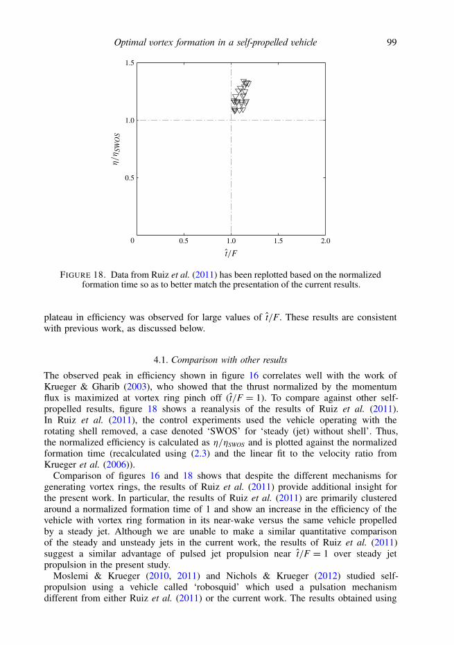
The observed peak in efficiency shown in figure 16 correlates well with the work ofKrueger & Gharib (2003), who showed that the thrust normalized by the momentumflux is maximized at vortex ring pinch off (t/F = 1). To compare against other self-propelled results, figure 18 shows a reanalysis of the results of Ruiz et al. (2011).In Ruiz et al. (2011), the control experiments used the vehicle operating with therotating shell removed, a case denoted ‘SWOS’ for ‘steady (jet) without shell’. Thus,the normalized efficiency is calculated as η/ηSWOS and is plotted against the normalizedformation time (recalculated using (2.3) and the linear fit to the velocity ratio fromKrueger et al. (2006)).

Comparison of figures 16 and 18 shows that despite the different mechanisms forgenerating vortex rings, the results of Ruiz et al. (2011) provide additional insight forthe present work. In particular, the results of Ruiz et al. (2011) are primarily clusteredaround a normalized formation time of 1 and show an increase in the efficiency of thevehicle with vortex ring formation in its near-wake versus the same vehicle propelledby a steady jet. Although we are unable to make a similar quantitative comparisonof the steady and unsteady jets in the current work, the results of Ruiz et al. (2011)suggest a similar advantage of pulsed jet propulsion near t/F = 1 over steady jetpropulsion in the present study.

Moslemi & Krueger (2010, 2011) and Nichols & Krueger (2012) studied self-propulsion using a vehicle called ‘robosquid’ which used a pulsation mechanismdifferent from either Ruiz et al. (2011) or the current work. The results obtained using


the robosquid vehicle showed that decreasing formation time yielded a monotonicincrease in the efficiency, in contrast with the present results. The discrepancy may berelated to the different mechanism of vortex ring formation in robosquid that created afully pulsed jet with greater enhancement of thrust. Krueger & Gharib (2003) showedthat over-pressurization of the nozzle exit during vortex ring formation is one of thecontributing factors to improving propulsive efficiency. It is likely that the robosquidvehicle, which uses a piston driven by a stepper motor to generate vortex rings, wasable to generate significant nozzle exit over-pressure, even at low formation times, asthe force generated by the accelerating flow was directly driven by a motor-drivenpiston. This is supported by the fact that the contribution of the nozzle exit over-pressure to the total impulse increases with decreasing formation time based on resultsfrom Krueger & Gharib (2003), who used a similar motor-driven piston mechanism.Thus, it is believed that the impulse from the nozzle exit over-pressure in the currentPVG-based vehicle is less than that generated by the motor-driven piston of robosquidfor low formation times. However, this theory cannot be confirmed by the currentresults as measurements of impulse generation during vortex ring ejection were nota part of the current study. It is also possible that differences in methods used tocalculate propulsive efficiency may also have contributed to the observed discrepanciesin the results. The robosquid efficiency results were obtained based on calculationsof the wake kinetic energy and thrust from digital particle image velocimetry (DPIV)measurements. This is in contrast to the method used presently.

4.2. Model predictionsRuiz et al. (2011) developed an analytical model for predicting the efficiency of apulsed-jet vehicle. Under various assumptions such as t/F < 1 and that the frequencyof oscillations f is sufficiently high such that ∂U∞/∂t ≈ 0, the efficiency of the vehicle,ηRWD, can be expressed as

ηRWD ≈ 23(1+ αxx)

U∞Uj, (4.1)

where αxx is the added mass coefficient for the forming vortex ring accelerating inthe axial direction of the flow. Using the dye visualizations of the vortex rings at theend of the pulsation cycle (cf. figure 17) the vortex bubble, defined as the volume offluid that moves with the vortex ring (Maxworthy 1972), can be obtained. In general,the vortex bubble is obtained through streamline analysis (Shariff & Leonard 1992;Dabiri & Gharib 2004), dye visualization (Shariff & Leonard 1992) or, more recently,Lagrangian coherent structures (LCS) (Shadden, Dabiri & Marsden 2006). Olcay &Krueger (2008) measured the vortex bubble size using all three methods. They foundthat in all cases, the dye method underestimated the vortex volume after completionof vortex ring formation and that the error increased in time. The increasing error wasdue to the vortex bubble volume increasing through ambient-fluid entrainment and thediffusion of vorticity, both of which are not reflected in dye visualization results.

While it is known that the volume of the vortex bubble will be underpredicted byusing the dye method, Olcay & Krueger (2008) show at the end of a pulsation cyclethat this error is, at worst, 10 % of the total volume and thus we assume that thisresults in a 5 % error in each lateral dimension of the vortex ring.

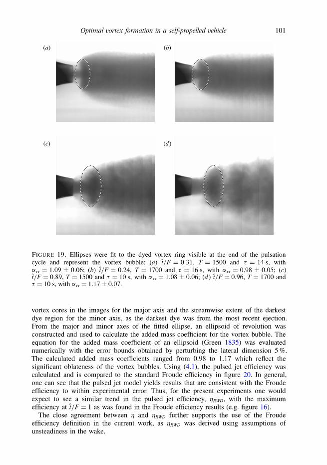
Under the assumption that the vortex ring can be modelled as an oblate ellipsoidof revolution, the resulting vortex bubbles are approximated using ellipses as shownin figure 19. The ellipses were fit by eye based on the approximate location of the


(a) (b)

(c) (d)

FIGURE 19. Ellipses were fit to the dyed vortex ring visible at the end of the pulsationcycle and represent the vortex bubble: (a) t/F = 0.31, T = 1500 and τ = 14 s, withαxx = 1.09 ± 0.06; (b) t/F = 0.24, T = 1700 and τ = 16 s, with αxx = 0.98 ± 0.05; (c)t/F = 0.89, T = 1500 and τ = 10 s, with αxx = 1.08 ± 0.06; (d) t/F = 0.96, T = 1700 andτ = 10 s, with αxx = 1.17± 0.07.

vortex cores in the images for the major axis and the streamwise extent of the darkestdye region for the minor axis, as the darkest dye was from the most recent ejection.From the major and minor axes of the fitted ellipse, an ellipsoid of revolution wasconstructed and used to calculate the added mass coefficient for the vortex bubble. Theequation for the added mass coefficient of an ellipsoid (Green 1835) was evaluatednumerically with the error bounds obtained by perturbing the lateral dimension 5 %.The calculated added mass coefficients ranged from 0.98 to 1.17 which reflect thesignificant oblateness of the vortex bubbles. Using (4.1), the pulsed jet efficiency wascalculated and is compared to the standard Froude efficiency in figure 20. In general,one can see that the pulsed jet model yields results that are consistent with the Froudeefficiency to within experimental error. Thus, for the present experiments one wouldexpect to see a similar trend in the pulsed jet efficiency, ηRWD, with the maximumefficiency at t/F = 1 as was found in the Froude efficiency results (e.g. figure 16).

The close agreement between η and ηRWD further supports the use of the Froudeefficiency definition in the current work, as ηRWD was derived using assumptions ofunsteadiness in the wake.


T

0

0.1

0.2

0.3

0.4

0.5

0.6

0.7

0.8

0.2 0.4 0.6 0.8 1.0

FIGURE 20. Pulsed jet efficiency, ηRWD, and the Froude efficiency, η, versus the normalizedformation time, t/F, for two values of T . The conditions plotted have their wake structuresand vortex bubbles shown in figure 19.

AcknowledgementsThe authors gratefully acknowledge the support of the Office of Naval Research

Grants N000140810918 and N000141010137 to J.O.D. In addition, the authors thankProfessor D. J. Stilwell and B. McCarter for providing the baseline AUV used in theseexperiments, and the reviewers for helpful comments on the work.

R E F E R E N C E S

BARTOL, I. K., KRUEGER, P. S., THOMPSON, J. T. & STEWART, W. J. 2008 Swimming dynamicsand propulsive efficiency of squids through ontogeny. Integr. Compar. Biol. 48 (6), 720–733.

BECKWITH, T. G., MARANGONI, R. D. & LIENHARD, J. H. 2007 Mechanical Measurements.Pearson Prentice Hall.

BERTRAM, C. D. 2003 Experimental studies of collapsible tubes. In Flow Past Highly CompliantBoundaries and in Collapsible Tubes, Fluid Mechanics and Its Applications, Vol. 72,pp. 51–65. Springer.

BERTRAM, C. D. & NUGENT, A. H. 2005 The flow field downstream of an oscillating collapsedtube. Trans. ASME: J. Biomech. Engng 127, 39–45.

BERTRAM, C. D., TRUONG, N. K. & HALL, S. D. 2008 Piv measurement of the flow field justdownstream of an oscillating collapsible tube. Trans. ASME: J. Biomech. Engng 130, 061011.

BERTRAM, C. D. & TSCHERRY, J. 2006 The onset of flow-rate limitation and flow-inducedoscillations in collapsible tubes. J. Fluids Struct. 22, 1029–1045.

CHOUTAPALLI, I. M. 2007 An experimental study of a pulsed jet ejector. PhD thesis, Florida StateUniversity.

CONRAD, W. A. 1969 Pressure-flow relationships in collapsible tubes. IEEE Trans. Biomed. EngngBME-16 (4), 284–295.

DABIRI, J. O. & GHARIB, M. 2004 Fluid entrainment by isolated vortex rings. J. Fluid Mech. 511,311–331.

DION, B., NAILI, S., RENAUDEAUX, J. P. & RIBEAU, C. 1995 Buckling of elastic tubes: study ofhighly compliant device. Med. Biol. Engng Comput. 33, 196–201.


FINLEY, T. J. & MOHSENI, K. 2004 Micro pulsatile jets for thrust optimization. In Proceedings ofIMECE2004, 2004 ASME International Mechanical Engineering Congress and Exposition.

FUNG, Y. C. 1997 Biomechanics: Circulation. Springer.GADRE, A. S., MACZKA, D. K., SPINELLO, D., MCCARTER, B. R., STILWELL, D. J., NEU, W.,

ROAN, M. J. & HENNAGE, J. B. 2008 Cooperative localization of an acoustic source usingtowed hydrophone arrays. In Autonomous Underwater Vehicles, 2008 (AUV 2008), pp. 1–8.IEEE/OES.

GHARIB, M., RAMBOD, E. & SHARIFF, K. 1998 A universal time scale for vortex ring formation.J. Fluid Mech. 360, 121–140.

GREEN, G. 1835 Researches on the vibration of pendulums in fluid media. Trans. R. Soc. Edinburgh13 (1), 54–62.

HEIL, M. 1996 The stability of cylindrical shells conveying viscous flow. J. Fluids Struct. 10,173–196.

HEIL, M. & JENSEN, O. E. 2003 Flows in deformable tubes and channels: theoretical models andbiological applications. In Flow Past Highly Compliant Boundaries and in Collapsible Tubes,Fluid Mechanics and Its Applications, Vol. 72, pp. 15–49. Springer.

HO, C.-M. & GUTMARK, E. 1987 Vortex induction and mass entrainment in a small-aspect-ratioelliptic jet. J. Fluid Mech. 179, 383–405.

KECECIOGLU, I., MCCLURKEN, M. E., KAMM, R. D. & SHAPIRO, A. H. 1981 Steady,supercritical flow in collapsible tubes. Part 1. Experimental observations. J. Fluid Mech. 109,367–389.

KRIEG, M. & MOHSENI, K. 2008 Thrust characterization of a bioinspired vortex ring thruster forlocomotion of underwater robots. IEEE J. Ocean. Engng 33 (2), 123–132.

KRIEG, M. & MOHSENI, K. 2010 Dynamic modelling and control of biologically inspired vortexring thrusters for underwater robot locomotion. IEEE Trans. Robot. 26 (3), 542–554.

KRIEG, M. & MOHSENI, K. 2013 Modelling circulation, impulse and kinetic energy of starting jetswith non-zero radial velocity. J. Fluid Mech. 719, 488–526.

KRUEGER, P. S. 2001 The significance of vortex ring formation and nozzle exit over-pressure topulsatile jet propulsion. PhD thesis, California Institute of Technology.

KRUEGER, P. S., DABIRI, J. O. & GHARIB, M. 2003 Vortex ring pinchoff in the presence ofsimultaneously initiated uniform background co-flow. Phys. Fluids 15 (7), L49–L52.

KRUEGER, P. S., DABIRI, J. O. & GHARIB, M. 2006 The formation number of vortex rings formedin uniform background co-flow. J. Fluid Mech. 556, 147–166.

KRUEGER, P. S. & GHARIB, M. 2003 The significance of vortex ring formation to the impulse andthrust of a starting jet. Phys. Fluids 15 (5), 1271.

KRUEGER, P. S. & GHARIB, M. 2005 Thrust augmentation and vortex ring evolution in afully-pulsed jet. AIAA J. 43 (4), 792–801.

LIEPMANN, D. & GHARIB, M. 1992 The role of streamwise vorticity in the near-field entrainmentof round jets. J. Fluid Mech. 245, 643–668.

LOVE, A. E. H. 1944 A Treatise on the Mathematical Theory of Elasticity. Dover.MAXWORTHY, T. 1972 The structure and stability of vortex rings. J. Fluid Mech. 51, 15–32.MOSLEMI, A. A. 2010 Propulsive efficiency of a biomorphic pulsed-jet underwater vehicle. PhD

thesis, Southern Methodist University.MOSLEMI, A. A. & KRUEGER, P. S. 2010 Propulsive efficiency of a biomorphic pulsed-jet

underwater vehicle. Bioinspir. Biomim. 5 (3), 036003.MOSLEMI, A. A. & KRUEGER, P. S. 2011 The effect of Reynolds number on the propulsive

efficiency of a biomorphic pulsed-jet underwater vehicle. Bioinspir. Biomim. 6 (2), 026001.MULLER, M. O., BERNAL, L. P., MORAN, R. P., WASHABAUGH, P. D., PARVIZ, B. A., CHOU,

T.-K. A., ZHANG, C. & NAJAFI, K. 2000a Thrust performance of micromachined syntheticjets. In AIAA Fluids 2000 Conference.

NICHOLS, J. T. & KRUEGER, P. S. 2012 Effect of vehicle configuration on the performance of asubmersible pulsed-jet vehicle at intermediate Reynolds number. Bioinspir. Biomim. 7 (3),036010.

OLCAY, A. B. & KRUEGER, P. S. 2008 Measurement of ambient fluid entrainment during laminarvortex ring formation. Exp. Fluids 44, 235–247.


PALERMO, T. & FLAUD, P. 1987 Etude de l’effondrement a deux et trois lobes de tubes elastiques.J. Biophys. Biomech. 11, 105–111.

PETRICH, J. 2009 Improved guidance, navigation, and control for autonomous underwater vehicles:theory and experiment. PhD thesis, Virginia Polytechnic Institute and State University.

PETRICH, J., NEU, W. L. & STILWELL, D. J. 2007 Identification of a simplified auv pitch axismodel for control design: theory and experiments. In OCEANS 2007, pp. 1–7.

PETRICH, J. & STILWELL, D. J. 2010 Model simplification for auv pitch-axis control design. OceanEngng 37 (7), 638–651.

PRANDTL, L. 1952 Essentials of Fluid Dynamics: With Applications to Hydraulics, Aeronautics,Meteorology and other Subjects. Hafner.

REYNOLDS, W. C., PAREKH, D. E., JUVET, P. J. D. & LEE, M. J. D. 2003 Bifurcating andblooming jets. Annu. Rev. Fluid Mech. 35, 295–315.

RUIZ, L. A., WHITTLESEY, R. W. & DABIRI, J. O. 2011 Vortex-enhanced propulsion. J. FluidMech. 668, 5–32.

SHADDEN, S. C., DABIRI, J. O. & MARSDEN, J. E. 2006 Lagrangian analysis of fluid transport inempirical vortex ring flows. Phys. Fluids 18, 047105.

SHARIFF, K. & LEONARD, A. 1992 Vortex rings. Annu. Rev. Fluid Mech. 24, 235–279.SIEKMANN, J. 1962 On a pulsating jet from the end of a tube, with application to the propulsion of

certain aquatic animals. J. Fluid Mech. 15 (03), 399–418.TRUONG, N. K. & BERTRAM, C. D. 2009 The flow field downstream of a collapsible tube during

oscillation onset. Commun. Numer. Meth. Engng 25, 405–428.WEIHS, D. 1977 Periodic jet propulsion of aquatic creatures. Forsch. Zool. 24, 171–175.

Documents

J. Fluid Mech. (2013), . 737, pp. doi:10.1017/jfm.2013.560