Embed Size (px)
Citation preview
J. Fluid Mech. (2013), vol. 720, pp. 104–139. c© Cambridge University Press 2013 104doi:10.1017/jfm.2012.640
The internal gravity wave field emitted by a stablystratified turbulent wake
Ammar M. Abdilghanie1 and Peter J. Diamessis2,†1Leadership Computing Facility, Argonne National Laboratory, Argonne, IL 60439, USA
2School of Civil and Environmental Engineering, Cornell University, Ithaca, NY 14853, USA
(Received 7 February 2012; revised 24 October 2012; accepted 19 December 2012)
The internal gravity wave (IGW) field emitted by a stably stratified, initially turbulent,wake of a towed sphere in a linearly stratified fluid is studied using fully nonlinearnumerical simulations. A wide range of Reynolds numbers, Re= UD/ν ∈ [5×10³, 105]and internal Froude numbers, Fr = 2U/(ND) ∈ [4, 16, 64] (U, D are characteristicbody velocity and length scales, and N is the buoyancy frequency) is examined. Atthe higher Re examined, secondary Kelvin–Helmholtz instabilities and the resultingturbulent events, directly linked to a prolonged non-equilibrium (NEQ) regime in wakeevolution, are responsible for IGW emission that persists up to Nt ≈ 100. In contrast,IGW emission at the lower Re investigated does not continue beyond Nt ≈ 50 for thethree Fr values considered. The horizontal wavelengths of the most energetic IGWs,obtained by continuous wavelet transforms, increase with Fr and appear to be smallerat the higher Re, especially at late times. The initial value of these wavelengths is setby the wake height at the beginning of the NEQ regime. At the lower Re, consistentwith a recently proposed model, the waves propagate over a narrow range of anglesthat minimize viscous decay along their path. At the higher Re, wave motion is muchless affected by viscosity, at least initially, and early-time wave propagation anglesextend over a broader range of values which are linked to increased efficiency inmomentum extraction from the turbulent wake source.
Key words: stratified flows, wakes/jets, waves/free-surface flows
1. IntroductionThe emission of internal gravity waves (IGWs) by submerged stably stratified
turbulence is a phenomenon of relevance to environmental/naval applications andfundamental stratified flow physics. The emitted waves can drive considerable energyredistribution within the water column (Thorpe 2005), are likely to amplify and breakcausing mixing far from the turbulent source (Keeler, Bondur & Gibson 2005)and can serve as an energy sink additional to viscous dissipation and diapycnalmixing within the turbulent source (Riley & Metcalfe 1987; Spedding 2002). Abroad body of literature dedicated to the study of IGW emission by stratifiedturbulence has revealed a phenomenon with extremely complex underlying physics.This complexity is compounded by the strong dependence of IGW and turbulenceproperties on the governing parameters, the degree of spatial localization of the source
† Email address for correspondence: [email protected]

Internal gravity waves emitted by stratified turbulent wakes 105
and whether the turbulent source is as stably stratified as the ambient fluid or iswell-mixed.
1.1. IGW radiation from turbulent mixed regions
We first review work on the radiation of IGWs from a well-mixed, continually forced,turbulent source into an overlying/underlying stably stratified portion of a host fluid.Such a flow configuration is representative of shear instabilities and turbulence inthe daytime atmospheric boundary layer and overlying convection-driven part ofthe troposphere exciting the stably stratified region above the tropopause (Townsend1965, 1968). It also is representative of equivalent motions in the oceanic mixed layer(Wijesekera & Dillon 1991; Moum et al. 1992) exciting the thermocline below it.Although fundamentally different from the emission of IGWs from a turbulent sourceembedded in a background stratification, where the turbulence follows a well-definedlifecycle (see § 1.2), IGW radiation from a well-mixed region has specific aspectswhich can provide critical insights into its fully stratified counterpart.
Linden (1975) studied the deepening of a mixing layer created at the top of astratified water tank by a vertically oscillating grid. Phase-line-tilt angles, defined asthe angle between the constant phase lines within a IGW and the vertical direction, ofthe waves radiated from the base of the mixed layer into the underlying stratificationwere found to have values of θ ≈ 35◦.
In a subsequent study, Sutherland & Linden (1998) examined experimentally andnumerically the excitation of IGWs by an unstable shear layer within a very weaklystratified layer overlying a stratified bottom layer. The phase-line-tilt angles werefound to be in the 45–60◦ range. The momentum transported by the waves led todeceleration of the mean flow by approximately 7 % of its characteristic flow speed.The accompanying two-dimensional direct numerical simulations (DNS) providedevidence that IGW radiation is indeed correlated with significant changes in themixed region dynamics. As a result, Sutherland & Linden hypothesized that thedominance of IGW excitation at 45◦ is the end result of a highly nonlinear feedbackbetween the waves and the turbulence in the mixed region which maximizes the dragon the associated mean flow. After observing turbulence-radiated IGWs prevailinglypropagating along a 45◦ angle in both a shear-free mixed layer (Dohan & Sutherland2003, 2005) and a turbulent wake of a towed laboratory-scale topography (Aguilar,Sutherland & Muraki 2006; Munroe & Sutherland 2008), Sutherland and coworkersultimately concluded that the properties of turbulence-generated IGWs are universal;that is, independent of the details of the turbulent source.
Taylor & Sarkar (2007) performed large-eddy simulations (LES) of a turbulentbottom Ekman layer which excited IGW radiation into an overlying stratification. Theradiated IGWs had phase-line tilt angles in the 35–60◦ range. A viscous decay-basedmodel was developed which predicted the rapid decay of high- and low-frequencycomponents of the initial wave spectrum whose content was dictated by the boundarylayer turbulence. Far from the turbulent source, the wave spectrum eventually peakedaround a dominant frequency set by the requirement of minimal viscous decay alongthe IGW propagation path. The DNS of Pham, Sarkar & Brucker (2009) of anunstable shear layer provided further support for the above viscous decay model; nearthe generation site, a relatively broad spectrum of propagation angles was observed,whereas, far from it, they found that the wave propagation angle was concentratedaround 45◦. Finally, 10 % of the initial shear layer momentum was estimated to betransported away by the radiated IGWs.
106 A. M. Abdilghanie and P. J. Diamessis
1.2. IGW radiation by localized stratified turbulence: stratified turbulent wakes1.2.1. The non-equilibrium regime in stratified wake evolution
The stratified turbulent wake of a towed sphere has emerged as the preferredprototype to investigate IGW emission by a localized turbulent region embedded in abackground stratification. The fundamental difference between this flow configurationand the well-mixed source set-up considered in the previous section is that the wave-generating turbulence is directly influenced by buoyancy and subject to a distinctlifecycle (Itsweire et al. 1993; Spedding 1997). In the parlance of stratified turbulentwakes, IGW radiation is focused in the non-equilibrium (NEQ) regime of wakeevolution (Spedding 2002). During this regime, the initially three-dimensional (3D)turbulence is subject to a complex adjustment to buoyancy effects before the flowultimately transitions into the quasi two-dimensional (Q2D) regime where the verticalvelocity field is negligible (Spedding 1997). As conjectured by Spedding (1997),restratification effects are responsible for converting the available potential energy,created by turbulence-induced overturning, into mean kinetic energy, as evidenced byreduced decay rates in the mean velocity defect (Gourlay et al. 2001; Dommermuthet al. 2002; Brucker & Sarkar 2010; Diamessis, Spedding & Domaradzki 2011).
In parallel, during the NEQ regime, some fraction of the wake’s energy is radiatedout by IGWs into the ambient fluid. While the mean wake profile continues to spreadin the lateral direction with the same growth rate as its unstratified counterpart, thewake height remains locked at the value corresponding to the onset of the NEQregime. In other words, the wake does not collapse, as proposed by other studies(Gilreath & Brandt 1985; Voisin 1991, 1994). Instead, within the wake, the verticalvorticity is concentrated in slowly evolving quasi-horizontal ‘pancake’ vortices. Thehorizontal vorticity is organized in highly diffuse and stable inclined layers (Spedding1997, 2002; Diamessis et al. 2011). The inclination of these layers is a result ofstraining by the mean velocity field (Spedding 2002). The layering, however, ofthe horizontal vorticity is strictly an effect of buoyancy, which provides strongercompressive strain in the vertical and biases the flow towards enhanced verticalvelocity gradients (Smyth 1999; Diamessis & Nomura 2000). No such vorticitylayering is observed in a turbulent flow in a non-stratified fluid (Gourlay et al. 2001).Hence, throughout this text, we will refer to the shear associated with these inclinedlayers as ‘buoyancy-driven’.
Both the quasi-horizontal pancake vortices and inclined shear layers are thedominant flow structures upon entry into the Q2D regime. For a given buoyancyfrequency, N, this transition occurs at Nt ≈ 50 according to the lower-Reynolds-numberexperiments of Spedding (1997). By this point, a balance between the centrifugal forceof the pancake eddies and the density and pressure fields is responsible for a nearlyundisturbed isopycnal field (Bonnier, Bonneton & Eiff 1998); any remaining IGWradiation has diminished significantly with respect to that which has occurred duringthe NEQ regime.
More recently, Diamessis et al. (2011, referred to herein as DSD) observed a visibleprolongation of the NEQ regime with increasing sphere Reynolds number Re= UD/ν,where U and D are the sphere tow speed and diameter and ν is the kinematicviscosity. This prolongation is intimately linked to the destabilization of the aboveinclined shear layers, whose thickness was found to decrease with Re whereas theirmagnitude increased. To this effect, secondary Kelvin–Helmholtz (K–H) instabilitiesand turbulence were observed up to Nt ≈ 100 for Re = 105. The persistent strongdisplacement of isopycnal surfaces induced by these secondary turbulent events is verylikely to drive IGW radiation over much longer intervals than those corresponding to

Internal gravity waves emitted by stratified turbulent wakes 107
laboratory experiments, which are conducted at Re typically an order of magnitudelower. A number of theoretical, laboratory and numerical studies, reviewed below,have examined the IGW emission by a stratified turbulent wake, although none hasspecifically examined the effect of Re on this phenomenon.
In the remainder of this manuscript, we differentiate between ‘low’ and ‘high’ Restratified turbulent wakes. High-Re stratified wakes are those which have an Re thatis sufficiently high, such as the value considered by DSD or even higher. Above thislimit Re, the above secondary K–H instabilities and turbulence occur within the wakecore. This set of distinct physical processes operating inside the wake core, linked tothe secondary phenomena, is absent in a low-Re stratified wake where any turbulenceinside the wake core is rapidly suppressed early into the NEQ regime. DSD showedthat the magnitude of the above buoyancy-driven shear layers scales as Re/Fr2, whereFr = 2U/(ND) is an internal Froude number. Therefore, at even higher Re, buoyancy-driven shear intensifies even further leading to even stronger secondary events and alonger NEQ regime.
1.2.2. Laboratory experimentsThe early shadowgraph-image-based experiments of Gilreath & Brandt (1985) of
a self-propelled body inside a stably stratified fluid distinguished two types of IGWobserved in the wake of the body: (a) deterministic, repeatable in apparently identicalrealizations of the experiment, body-generated/lee waves and short-lived transientwaves generated by the swirling motion of the propeller; and (b) non-deterministicIGWs, characterized as random by the authors, that are emitted by the turbulent wakeemerging during what is regarded as a wake collapse. This collapse was proposedto occur once the large-scale turbulent bursts/puffs on the wake boundary cease togrow on account of the continuously increasing influence of buoyancy forces in thedownstream direction.
The turbulent kinetic energy of the wake was hypothesized to be transferredinto available potential energy and hence to random IGWs when a local turbulentFroude number, based on the r.m.s. turbulent velocity and the turbulent integral scale,approaches unity. Linear theory was found to successfully predict the amplitude of thedeterministic component of the IGW field but not that of the random component onaccount of its highly complex turbulent wake source (see § 1.2.1).
Bonneton, Chomaz & Hopfinger (1993, referred to herein as BCH) used a custom-designed laser-induced fluorescence technique (Hopfinger et al. 1991) to measurethe IGW-driven isopycnal displacement on a horizontal plane beneath the turbulentwake core. Over the range of sphere-based Reynolds numbers, Re ∈ [380, 3 × 10⁴],considered, the observed IGW field transitioned from a lee-wave-dominated to arandom-wave-dominated field at Fr ≈ 4.5, independent of Re. At the same Fr , IGWemission persisted for a much longer time when Re was increased by a factor of ten.
BCH also suggested that the random IGW wavelength decreases roughly as 1/Nt, inagreement with impulsive source theory (Lighthill 1978; Zavol’Skii & Zaitsev 1984;Voisin 1991, 1994). Nonetheless, their results are subject to large scatter and visualinspection of their cloud of data points suggests an actual decrease at a rate quiteslower than 1/Nt. Moreover, when one graphically computes the slope of the linetangent to the top and bottom edge of the cloud of data points in figure 8 of BCH, apower law of Ntα with α ∈ [−0.4 −0.7] is inferred.
The waves arriving first at the measurement plane of BCH had a horizontalwavelength of λH ∈ [1.5D, 2D] with a phase-line tilt angle of θ = 55◦. Such a valueof θ maximizes the wave-induced isopycnal displacement amplitude according to

108 A. M. Abdilghanie and P. J. Diamessis
Lighthill’s theory for IGWs generated by a point disturbance. In this regard, whena model of a mixed region collapsing in a uniformly stratified fluid is considered aswave source, the solution of the linearized IGW equations shows that the isopycnaldisplacement amplitude of the radiated IGWs is maximized along θ = 38◦ (Meng &Rottman 1988). However, this model is rather unlikely to be applicable to the wakeof a towed sphere because of the relatively weak mixing observed inside the wake (cf.Brucker & Sarkar 2010).
Robey (1997) towed a sphere along the base of the thermocline of a two-layer fluid.Results from a numerical model, based on the linearized equations of motion, wheresphere and wake motion were represented by a distribution of sources and sinks, werealso examined. For the wake-generated random waves, the source was assumed to bea large-scale turbulent eddy with characteristic scales (velocity, length and diameter)that were estimated on the basis of resonance between the eddies and the stratification.The model produced reasonable agreement with the experimentally determined wavedisplacement amplitude.
Spedding et al. (2000) examined the structure and properties of the IGW fieldradiated by a towed sphere in a linearly stratified fluid. Two-dimensional wavelettransforms were used to analyse particle image velocimetry (PIV) data sampled ona horizontal plane above the wake centreline. An Fr1/3 scaling, derived from theevolution of the average horizontal eddy dimensions (Spedding, Browand & Fincham1996), was found to partially collapse the time series of horizontal wavelengths.
1.2.3. Theoretical modelsBeyond the theories that successfully predict the geometry of body-generated
deterministic waves and the waves generated by a moving point source (Miles 1971;Peat & Stevenson 1975; Lighthill 1978; Chashechkin 1989) in a stratified fluid,two sets of theoretical studies provide a preliminary explanation of the origin ofthe random component of the IGW field from within the turbulence along with aprediction of some its spectral characteristics. Relying on a spectrally based theory forthe lifecycle of a stratified turbulent patch, Gibson (1980) suggested that large-scaleturbulent eddies transfer their kinetic energy to IGWs when the largest isopycnaloverturning scale inside the patch is equal to the Ozmidov scale,
LO ≡ (ε/N3)1/2, (1.1)
where ε is the turbulent kinetic dissipation rate (Dougherty 1961; Ozmidov 1965).This transition point in the evolution of a stratified turbulent patch is regarded asthe ‘beginning of fossilization’ by Gibson or ‘onset of buoyancy control’ by others(Itsweire et al. 1993). It effectively corresponds to the beginning of the NEQ regimein the evolution of a stratified turbulent wake (Spedding 1997). According to Gibson,the patch-radiated waves have a wavelength equal to the value of LO at this time and afrequency close to N.
The experimental studies of Wu (1969) and Gilreath & Brandt (1985), and theirclaim that the collapse of individual density/velocity disturbances in a stratified fluidmay serve as impulsive sources of IGWs, served as the springboard for the theoreticalwork by Voisin (1991, 1994). Voisin thus modelled IGW radiation from a turbulentwake as a process driven by a discrete distribution of impulsive sources and sinkswhich are periodically spaced in both space and time and represent a collection ofturbulent puffs resulting from the collapse of connected vortex loops within the wake.The theory predicted that the wavelength of an IGW decreases as 1/Nt and thatthe phase-line-tilt angle θ = 55◦ maximizes wave displacement amplitude that itself

Internal gravity waves emitted by stratified turbulent wakes 109
increases according to√
Nt. However, the theory did not predict the value of thewavelength itself or its possible Re and Fr scaling.
Finally, a relevant study is that by Plougonven & Zeitlin (2002) on IGW emissionfrom an idealized inviscid pancake vortex model which exploits similarities with soundwave emission by unsteady vortex motion in a compressible fluid (Lighthill 1952). Inthis model, wave emission was found to have a significant impact on the source vortex,eventually leading to its destabilization.
1.2.4. Numerical simulationsOnly a limited number of computational studies have considered the IGW field
radiated by localized turbulence in a stratified fluid. Druzhinin (2009) performednumerical simulations of a stratified jet. Two values of Reynolds number, based onthe jet diameter and centreline velocity, of 400 and 700 were considered at verylow Fr ∈ [0.3, 2.5]. Graphical estimates from two-dimensional transects yielded aphase-line tilt angle of 53◦ to the vertical.
Finally and more recently, de Statler, Sarkar & Brucker (2010) performed DNSof a stratified turbulent wake at Re = 104, where three values of Prandtl number,Pr = ν/κ = 0.2, 1 and 7 were examined (where κ is the mass diffusivity). At thelowest value of Pr, the enhanced diffusion within the density field caused a significantreduction in IGW energy flux into the ambient. In contrast, only subtle variation wasobserved in the IGW energy flux for the more geophysically relevant values of Pr = 1and 7.
1.3. Outstanding issuesDespite the valuable insights provided by previous studies on the wake-radiatedIGW field, a number of critical aspects of this phenomenon have not yet beenaddressed. The localization of the wake in the transverse direction manifests itselfin an equivalent localization of the wake-radiated IGW field on any observation planevertically offset sufficiently far from the wake centreline. Estimation of the spectralproperties of the IGWs is realizable a lot more efficiently by using the wavelettransforms and their localized basis functions, which provide output in both physicaland spectral space (Dallard & Spedding 1993).
The pioneering experimental studies of Gilreath & Brandt (1985) and BCH reportedquantitative IGW data at only a few isolated locations in their experimental facilities.The variation in properties of the IGW field in the transverse and vertical direction,resulting from its corresponding inhomogeneity, needs to be explored while exploitingthe associated streamwise homogeneity to extract reliable statistical descriptions of thequantities of interest.
Additionally, a broader range of Re and Fr values over which random wavesdominate the radiated IGW field needs to be examined. On one hand, on account ofrestrictions of the associated experimental facilities, BCH and Robey (1997) limitedtheir Fr to the intervals [4.5, 12.7] and [4, 22], respectively. On the other hand,Gilreath & Brandt (1985) considered only one Fr value. Spedding et al. (2000)examined a broader range of Fr but provided only a preliminary analysis of theradiated IGW field. In a similar vein, presumably constrained by limitations in theexperimental facility (BCH; Spedding 1997), the above laboratory studies were notable to significantly vary Re. The numerical studies of Druzhinin (2009) and de Statleret al. (2010) were also restricted to a relatively low Re value. As indicated in § 1.2.1,the prolongation of the NEQ regime at higher Re has implications for various aspectsof wake structure and dynamics.
110 A. M. Abdilghanie and P. J. Diamessis
1.4. Objectives and basic questions
Motivated by the above discussion, the primary objective of this study is tocharacterize the IGW field over a range of Re and Fr that is considerably broader thanthat considered in previous studies. To this end, it is of primary interest to determinewhether the extended duration of the NEQ regime at high Re results in a prolongationof IGW radiation, through the persistent excitation of the isopycnals by secondaryturbulence. Note that hereafter any reference to persistent excitation of isopycnals orpersistent IGW radiation indicates that these phenomena last much longer than they doin low-Re wakes.
In addition, on account of the dynamically evolving turbulent wake structure duringthe NEQ regime, this work aims to assess the potential impact of increased Re,and the increasingly inviscid dynamics inside the wake, on the spatial structure,wavelengths, frequencies and amplitudes of IGWs in the near field. Although thespectral properties of the radiated waves far from their source are critically important,simulations which can accurately resolve both the wake turbulence and the far field ofradiated IGWs are prohibitively costly and deferred to future studies.
Some specific questions include: Is IGW radiation a transient phenomenon, in theform of short-lived impulsive bursts, or does it occur in a more continuous/quasi-steady manner? If the latter is true, is it dependent on the duration of the NEQ regime(or Re for that matter)? What is the dependence of IGW wavelength magnitude andits rate of decrease on Re and Fr? Is there any plausible Re and Fr scaling forthese wavelengths that is traceable to a corresponding scaling for the turbulent sourcecharacteristics? Do the IGW wavelengths decrease in agreement with the impulsivesource theory? Does the preferred IGW phase-line tilt angle change with increasing Reand, if yes, does such a change denote a transition from a wave radiation process thatis viscously controlled to a more inviscid one that maximizes momentum extractionfrom the wake?
2. Model formulationThe base flow considered in this study is identical to that considered in DSD.
This section discusses the most important features of base flow geometry. The readerinterested in more detail, especially in the context of design and implementation ofinitial conditions, is referred to DSD. The few subtle differences in simulation set-upbetween this work and DSD are discussed at the end of § 4.
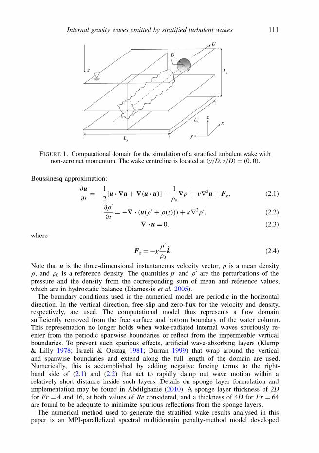
Specifically, we examine a stratified turbulent wake with non-zero net momentum.Such a flow corresponds to the wake of a sphere of diameter D towed with avelocity U in a uniformly stratified fluid with buoyancy frequency N; see figure 1. Asimplemented by Orszag & Pao (1975) and in more recent studies of stratified turbulentwakes (Gourlay et al. 2001; Dommermuth et al. 2002; Diamessis, Domaradzki& Hesthaven 2005; Brucker & Sarkar 2010, DSD), on account of challenges ofcomputational complexity, the computational domain and spatial discretization do notaccount for the sphere and focus only on the flow generated in its wake. Specifically,the computational domain is a fixed three-dimensional volume, of dimensionsLx × Ly × Lz, inside the wake region centred on the wake centreline. The sphereis considered to have already travelled through the computational domain, movingin the rightward direction. The wake centreline corresponds to (y/D, z/D) = (0, 0).Within the computational domain, the three-dimensional and time-dependent wake flowfield is computed by solving the incompressible Navier–Stokes equations under the
Internal gravity waves emitted by stratified turbulent wakes 111
g
Ly
Lx
Lz
U
D
xz
y
FIGURE 1. Computational domain for the simulation of a stratified turbulent wake withnon-zero net momentum. The wake centreline is located at (y/D, z/D)= (0, 0).
Boussinesq approximation:
∂u∂t=−1
2[u ·∇u+∇(u ·u)] − 1
ρ0∇p′ + ν∇2u+ Fg, (2.1)
∂ρ ′
∂t=−∇ · (u(ρ ′ + ρ(z)))+ κ∇2ρ ′, (2.2)
∇ ·u= 0. (2.3)
where
Fg =−gρ ′
ρ0k̂. (2.4)
Note that u is the three-dimensional instantaneous velocity vector, ρ is a mean densityρ, and ρ0 is a reference density. The quantities p′ and ρ ′ are the perturbations of thepressure and the density from the corresponding sum of mean and reference values,which are in hydrostatic balance (Diamessis et al. 2005).
The boundary conditions used in the numerical model are periodic in the horizontaldirection. In the vertical direction, free-slip and zero-flux for the velocity and density,respectively, are used. The computational model thus represents a flow domainsufficiently removed from the free surface and bottom boundary of the water column.This representation no longer holds when wake-radiated internal waves spuriously re-enter from the periodic spanwise boundaries or reflect from the impermeable verticalboundaries. To prevent such spurious effects, artificial wave-absorbing layers (Klemp& Lilly 1978; Israeli & Orszag 1981; Durran 1999) that wrap around the verticaland spanwise boundaries and extend along the full length of the domain are used.Numerically, this is accomplished by adding negative forcing terms to the right-hand side of (2.1) and (2.2) that act to rapidly damp out wave motion within arelatively short distance inside such layers. Details on sponge layer formulation andimplementation may be found in Abdilghanie (2010). A sponge layer thickness of 2Dfor Fr = 4 and 16, at both values of Re considered, and a thickness of 4D for Fr = 64are found to be adequate to minimize spurious reflections from the sponge layers.
The numerical method used to generate the stratified wake results analysed in thispaper is an MPI-parallelized spectral multidomain penalty-method model developed
112 A. M. Abdilghanie and P. J. Diamessis
to simulate incompressible high Reynolds-number localized stratified turbulence inhorizontally periodic and vertically finite domains. Details on the numerical modelmay be found in Diamessis et al. (2005) and DSD. Through the multidomain scheme,resolution is concentrated on the wake core and the larger-scale turbulent motionswithin it, which include the secondary K–H instabilities and turbulence at high Re thatsustain persistent IGW radiation. Away from the wake core, the subdomain thicknessbecomes larger, though adequate to resolve the relevant length scale of interest, thevertical wavelength of the IGW field which is O(D).
3. Continuous wavelet transform (CWT)The Fourier transform, on account of its globally defined periodic basis functions,
is best suited for (nearly) monochromatic signals where the spectral content of thesignal does not change over space or time. It has proven useful in previous analysesof IGW fields emitted from forced turbulent sources (Sutherland, Flynn & Dohan2004; Aguilar & Sutherland 2006; Taylor & Sarkar 2007; Munroe & Sutherland 2008).However, it is of limited use for wave fields whose frequency (wavenumber) contentchanges over time (space). The localized nature of the wake-generated IGW field isdue to the spatial localization of the wake core itself in the vertical and transversedirections and the finite duration of any vertical turbulent motions within the wakedue to buoyancy-driven decay (Diamessis, Gurka & Liberzon 2010). The temporallocalization is mainly evident in low-Re wakes.
In one dimension, the CWT of a continuous temporal signal x(t) with respect to awavelet basis function (or mother wavelet) ψ(t) is defined as
T(a, b)= 1√a
∫ ∞−∞
x(t)ψ∗(
t − b
a
)dt, (3.1)
where the asterisk denotes the complex conjugate of an analysing wavelet that isobtained from a mother wavelet ψ(t) through translation to a location b and stretchingby a factor a. By virtue of its localized basis functions, the CWT retains informationin both physical and spectral domain at optimal resolution (Dallard & Spedding 1993).Large values of the CWT modulus T(a, b) signify resonance between signal and theanalysing wavelet at the corresponding scale.
The wavelength of the IGWs is extracted using either of two complex two-dimensional wavelet basis functions as defined by Dallard & Spedding (1993). Thefirst mother wavelet, Morlet2D, is direction-specific. It selects localized wavenumbervectors with a preferred magnitude and orientation. The second wavelet basis function,Arc, is regarded as cylindrical; it has no directional selectivity and hence resonateswith wavenumber vectors of a particular magnitude regardless of orientation. Finally,the one-dimensional CWT based on the complex Morlet wavelet (Addison 2002)is used to extract the frequency content of time series obtained at multiple spatiallocations.
4. Summary of numerical simulationsThis study considers results from five different numerical simulations: at Reynolds
number Re = 5 × 10³ for Froude number Fr = 4, 16 and 64, and at Re = 105 forFr = 4 and 16. DSD examined the same parameter values, augmented by one moresimulation at Re = 105 and Fr = 64. Hereafter, each run is labelled as RxFy, wherex= Re/103 and y= Fr . As in DSD, for all simulations, the values of U and D are the
Internal gravity waves emitted by stratified turbulent wakes 113
same. The Reynolds number and Froude number are varied by changing the values ofν and N, respectively.
All simulations are run up to Nt = 100, by which time, at low Re, the wake core iswell within the Q2D regime (Spedding 1997, DSD;). At high Re, very few secondaryK–H instabilities survive beyond Nt = 100 (DSD), at which point IGW radiationbegins to significantly diminish.
To unambiguously determine the IGW-field spectral characteristics, thecomputational domain dimensions should be large enough to allow adequate distancefor the IGWs to freely propagate away from the wake core, thereby preventing anycontamination of the wave field analysis by the wake turbulence. At Fr = 4 and 16,for both Re, the domain in this study has dimensions Lx × Ly × Lz = 26(2/3)D ×26(2/3)D×12D. The Fr = 64 case uses domain dimensions of 26(2/3)D×40D×20Dto account for a broader and taller wake during the time intervals of interest.
The choice of the dimensions of the domain in this study is sufficient to enablereliable estimation of the near-field properties of the radiated IGW field and directcomparison of our results to the experiments of BCH. ‘Near field’ here denotesthat the IGW field is sampled at locations which range between one to two spherediameters away from the vertical location of the edge of the turbulent wake, estimatedbased on the wake half-height values provided by DSD. Investigating the far-fieldproperties of the IGWs requires much deeper domains giving rise to a significant andprohibitive increase in computational cost.
Across all runs, the computational grids are nearly identical with those used byDSD for the equivalent parameter values (see their figure 3 for an example). For bothFr = 4 and 16, the resolutions at Re = 5 × 10³ and 105 are 256 × 256 × 175 and512 × 512 × 531 mesh points, respectively. In this regard, the only difference withDSD is the use of double the number of mesh points, though equal resolution per unitlength, in the spanwise direction with respect to DSD. The Re = 5 × 10³ and Fr = 64case uses a resolution of 256× 384× 225 to accommodate a taller and deeper domain.An equivalent increase in resolution at Re = 105 for Fr = 64 requires an increasein resolution that exceeds the memory capacity per processor of the Arctic RegionSupercomputing Center’s Midnight cluster used to perform the simulations consideredhere. We have thus deferred such a simulation to future, longer-term, efforts. Finally,the spectral filters used for each value of Re and Fr are the same as those employedby DSD (see their figure 4).
Adequate resolution of the turbulent wake core for all the simulations consideredhere has already been demonstrated in DSD, both in terms of the scale of the inclinedshear layers and the resulting primary two-dimensional stage of the Kelvin–Helmholtzinstabilities and subsequent billow pairing. For details, see the relevant discussion onpp. 68 and 78–79 of that paper. Therefore, any IGW-generating motions inside thewake core are well-resolved. Moreover, the IGW wavelengths, as computed in § 5.2below and inferred from the visualizations of figures 3–6, are also well-resolved.
Finally, we emphasize that subtle differences exist between the simulations reportedhere and those reported in DSD. The simulations considered in this paper use widerand, for Fr = 64, deeper domains than DSD. In addition, sponge layers wrap aroundthe lateral and top/bottom boundaries of the domain. The simulations are run only upto Nt = 100, times where IGW radiation is significant for the higher Re considered.The regridding used by DSD is not employed here. Whereas the regridding strategyused by DSD enabled them to run as far as Nt ≈ 2000, the lack of sponge layers intheir simulations and the application of the first regridding at times where the radiated
114 A. M. Abdilghanie and P. J. Diamessis
IGWs had already re-entered from the periodic boundaries do not allow a reliableexamination of the IGW field in the DSD dataset.
5. Results5.1. Visualization of the wave field structure
Following the preliminary study of Spedding et al. (2000), the fundamental quantityin the visualization and analysis of the wake-radiated IGW field performed here is thehorizontal divergence of the velocity field
1z ≡∇ ·uH, (5.1)
where uH ≡ (u, v) is the horizontal velocity vector. If Fr l represents a local Froudenumber, based on the local integral scale of the turbulence and the r.m.s. of thevelocity fluctuations, then in the very low-Fr l limit, as indicated by Spedding et al.(1996) and according to the decomposition of Riley, Metcalf & Weissman (1981)and Lilly (1983), 1z enables an exact separation of internal wave motions with timescales of O(N−1) and amplitudes in z of O(1) from turbulent motions, namely vorticalmodes, with time scales O(N−1/Fr l) and vertical motion of amplitude O(Fr2
l ) inz. In the flows considered here, even if Fr l may be relatively large at early times,indicating a weak influence of buoyancy, it eventually attains a small value signifyingfull buoyancy control over the turbulent motion inside the wake. Thus, 1z is anapproximate, though highly convenient, descriptor of the IGW field.1z may be related to the IGW-driven vertical isopycnal displacement amplitude field
in a straightforward way. For small-amplitude IGW field with horizontal and verticalwavenumbers, κH and m, and frequency ω in a uniformly stratified fluid (Sutherland2010),
|Aζ | = |A1z |mω
, (5.2)
where A1z is the amplitude of the horizontal divergence field and Aζ is the isopycnaldisplacement amplitude. Since the vertical wavenumber is related to the horizontalone by m = κH tan(θ) and by virtue of the linear internal wave dispersion relation,ω = N cos(θ), the isopycnal displacement amplitude is therefore proportional to A1z/N.Moreover, for IGWs subject to a relatively narrow range of propagation angles,the factor κH tan(θ) cos(θ) may be treated as constant. Therefore, normalizing thehorizontal divergence field by the buoyancy frequency then provides an approximatemeasure for the isopycnal displacement of the wave field.
In the remainder of this paper, any discussion of IGW-induced isopycnaldisplacement will be limited to qualitative assessment of the visualizations pertinentto this section. The wave steepness, a measure of wave nonlinearity (Sutherland 2010),may be readily obtained by normalizing the maximum isopycnal displacement bythe horizontal wavelength of the IGW. More quantitative analysis of the steepnessof the IGW field examined here is the subject of ongoing research. For preliminaryresults on the evolution of wave steepness in the simulations considered here and theimplications of these results for the potential for destabilization of the radiated IGWs(Sutherland 2001), the interested reader is referred to Abdilghanie (2010).
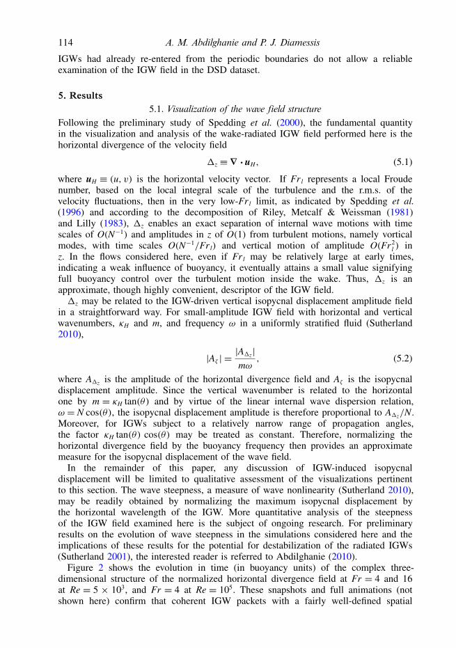
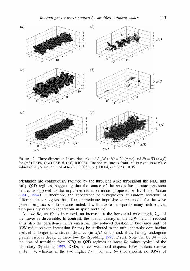
Figure 2 shows the evolution in time (in buoyancy units) of the complex three-dimensional structure of the normalized horizontal divergence field at Fr = 4 and 16at Re = 5 × 10³, and Fr = 4 at Re = 105. These snapshots and full animations (notshown here) confirm that coherent IGW packets with a fairly well-defined spatial
Internal gravity waves emitted by stratified turbulent wakes 115
50
–5–5
–10
05
10
–202
–4
4
50
–5
–5–10
05
10
–202
–4
4
50
–5
–5–10
05
10
–202
–4
4
50
–5
–5–10
05
10
–202
–4
4
50
–5
–5–10
05
10
–202
–4
4
50
–5–5
–10
05
10
–202
–4
4
(a) (b)
(c) (d )
(e) ( f )
FIGURE 2. Three-dimensional isosurface plot of 1z/N at Nt = 20 (a,c,e) and Nt = 50 (b,d,f )for (a,b) R5F4, (c,d) R5F16, (e,f ) R100F4. The sphere travels from left to right. Isosurfacevalues of 1z/N are sampled at (a,b) ±0.025, (c,d) ±0.04, and (e,f ) ±0.05.
orientation are continuously radiated by the turbulent wake throughout the NEQ andearly Q2D regimes, suggesting that the source of the waves has a more persistentnature, as opposed to the impulsive radiation model proposed by BCH and Voisin(1991, 1994). Furthermore, the appearance of wavepackets at random locations atdifferent times suggests that, if an approximate impulsive source model for the wavegeneration process is to be constructed, it will have to incorporate many such sourceswith possibly random separations in space and time.
At low Re, as Fr is increased, an increase in the horizontal wavelength, λH , ofthe waves is discernible. In contrast, the spatial density of the IGW field is reducedas is also the persistence in its emission. The reduced duration in buoyancy units ofIGW radiation with increasing Fr may be attributed to the turbulent wake core havingevolved a longer downstream distance (in x/D units) and, thus, having undergonegreater viscous decay, at these low Re (Spedding 1997, DSD). Note that by Nt = 50,the time of transition from NEQ to Q2D regimes at lower Re values typical of thelaboratory (Spedding 1997, DSD), a few weak and disperse IGW packets surviveat Fr = 4, whereas at the two higher Fr = 16, and 64 (not shown), no IGWs of
116 A. M. Abdilghanie and P. J. Diamessis
(a)
(b)
(c)
15 30 50
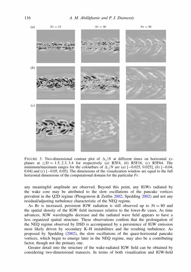
FIGURE 3. Two-dimensional contour plot of 1z/N at different times on horizontal xy-planes at z/D = 1.5, 2.3, 3.4 for respectively (a) R5F4, (b) R5F16, (c) R5F64. Theminimum/maximum ranges for the colourbars of 1z/N are (a) [−0.025, 0.025], (b) [−0.04,0.04] and (c) [−0.05, 0.05]. The dimensions of the visualization window are equal to the fullhorizontal dimensions of the computational domain for the particular Fr .
any meaningful amplitude are observed. Beyond this point, any IGWs radiated bythe wake core may be attributed to the slow oscillations of the pancake vorticesprevalent in the Q2D regime (Plougonven & Zeitlin 2002; Spedding 2002) and not anyresidual/adjusting turbulence characteristic of the NEQ regime.
As Re is increased, persistent IGW radiation is still observed up to Nt = 80 andthe spatial density of the IGW field increases relative to the lower-Re cases. As timeadvances, IGW wavelengths decrease and the radiated wave field appears to have aless organized spatial structure. These observations confirm that the prolongation ofthe NEQ regime observed by DSD is accompanied by a persistence of IGW emissionmost likely driven by secondary K–H instabilities and the resulting turbulence. Asproposed by Spedding (2002), the slow oscillations of the quasi-horizontal pancakevortices, which begin to emerge later in the NEQ regime, may also be a contributingfactor, though not the primary one.
Greater detail into the structure of the wake-radiated IGW field can be obtained byconsidering two-dimensional transects. In terms of both visualization and IGW-field

Internal gravity waves emitted by stratified turbulent wakes 117
(a)
(b)
15 30 50
FIGURE 4. Two-dimensional contour plot of 1z/N at different times in the range 15 < Nt <50 on horizontal xy-planes at z/D = 1.5, 2.3, for respectively (a) R100F4, (b) R100F16.The minimum/maximum ranges for the colourbars of 1z/N are (a) [−0.05, 0.05], (b)[−0.075, 0.075]. For each Fr, the size of the visualization window is the same as in thecorresponding Re= 5× 10³ contour plots in figure 3.
analysis, we focus on xy-planes vertically offset from the wake centreplane (figures3–5). These planes are free of motions from the turbulent wake core, are optimalfor two-dimensional wavelet analysis (see §§ 3 and 5.2) and enable a straightforwardcomparison with the experimental results of BCH and Spedding et al. (2000). Here,unlike figure 2, we show visualizations from all Re and Fr examined to enable afull comparison of the radiated IGW-field geometry across all values of the governingparameters considered.
According to figure 3, the amplitude of the normalized horizontal divergence fieldincreases with Fr . This increase of amplitude with reduced stratification strengthindicates, by virtue of (5.2), that the isopycnal displacement amplitude may alsoincrease. For the same Fr , by contrasting figures 3–5, one also observes a significantincrease in the amplitude of the normalized horizontal divergence field with increasingRe.
The evolution and structure of the wave field in figure 3, for Re = 5 × 10³, is verysimilar to that observed by Spedding et al. (2000) for their Fr > 4 cases wherethe random wake-generated component dominates the wave field. Consistently withfigure 2, at low Re, IGW radiation is a short-lived process; wave emission begins earlyin the NEQ regime and continues until the flow transitions into the Q2D regime, theapproximate transition point identified by DSD. In contrast, at high Re (figures 4 and5), the emission of energetic IGW packets persists as late as Nt ≈ 90 and Nt ≈ 70for runs R100F4 and R100F16, respectively. For the Fr = 4 runs, a correspondingsequence of snapshots at z/D = 3 (not shown here) reveals no wave activity up
118 A. M. Abdilghanie and P. J. Diamessis
(a)
(b)
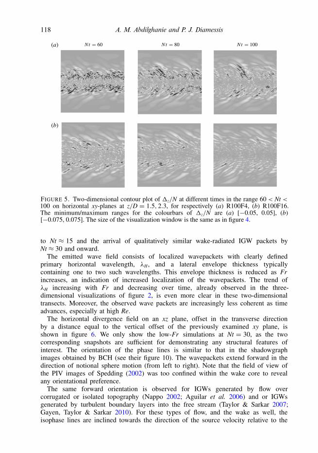
60 80 100
FIGURE 5. Two-dimensional contour plot of 1z/N at different times in the range 60 < Nt <100 on horizontal xy-planes at z/D = 1.5, 2.3, for respectively (a) R100F4, (b) R100F16.The minimum/maximum ranges for the colourbars of 1z/N are (a) [−0.05, 0.05], (b)[−0.075, 0.075]. The size of the visualization window is the same as in figure 4.
to Nt ≈ 15 and the arrival of qualitatively similar wake-radiated IGW packets byNt ≈ 30 and onward.
The emitted wave field consists of localized wavepackets with clearly definedprimary horizontal wavelength, λH , and a lateral envelope thickness typicallycontaining one to two such wavelengths. This envelope thickness is reduced as Frincreases, an indication of increased localization of the wavepackets. The trend ofλH increasing with Fr and decreasing over time, already observed in the three-dimensional visualizations of figure 2, is even more clear in these two-dimensionaltransects. Moreover, the observed wave packets are increasingly less coherent as timeadvances, especially at high Re.
The horizontal divergence field on an xz plane, offset in the transverse directionby a distance equal to the vertical offset of the previously examined xy plane, isshown in figure 6. We only show the low-Fr simulations at Nt = 30, as the twocorresponding snapshots are sufficient for demonstrating any structural features ofinterest. The orientation of the phase lines is similar to that in the shadowgraphimages obtained by BCH (see their figure 10). The wavepackets extend forward in thedirection of notional sphere motion (from left to right). Note that the field of view ofthe PIV images of Spedding (2002) was too confined within the wake core to revealany orientational preference.
The same forward orientation is observed for IGWs generated by flow overcorrugated or isolated topography (Nappo 2002; Aguilar et al. 2006) and or IGWsgenerated by turbulent boundary layers into the free stream (Taylor & Sarkar 2007;Gayen, Taylor & Sarkar 2010). For these types of flow, and the wake as well, theisophase lines are inclined towards the direction of the source velocity relative to the

Internal gravity waves emitted by stratified turbulent wakes 119
(a)
(b)
FIGURE 6. Two-dimensional contour plot of 1z/N at Nt = 30 on the vertical xz-plane aty/D = 1.5 for (a) R5F4, (b) R100F4. The minimum/maximum ranges for the colourbars of1z/N are (a) [−0.025, 0.025], (b) [−0.05, 0.05]. The visualization window has dimensions26 2/3D× 12D and is centred around z/D= 0.
free-stream velocity. In the case of the wake, given the absence of any currents in theambient fluid, this direction is that of the mean wake velocity profile, a direct resultof the unidirectional forcing by the towed sphere. In other words, the advection of thewake-generating structures by the mean wake profile is the only way by which fore–aftsymmetry is broken in this problem (Geoffrey Spedding, personal communication).
Finally, for both simulations at Fr = 4, the continued lateral expansion of the wakecore is responsible for the emergence in the field of view of figure 6 of either nearlyhorizontal features, presumably linked to inclined horizontal vorticity layers (DSD),(low Re) or small-scale turbulence (high Re).
5.2. Spectral characteristics of the IGW field
The basis of our analysis of the IGW-field spectral characteristics is the application oftwo-dimensional wavelet transforms on the horizontal divergence field sampled on xyplanes vertically offset above the wake centreline. In each simulation, these analysisplanes are those examined in the visualizations of figures 3–5. At a given time, asingle two-dimensional xy transect is found to provide sufficient information on thespanwise variability of the wake-radiated IGW field. Details on the computation of thehorizontal wavelength via two-dimensional wavelets from the xy transects are providedin appendix A.
5.2.1. Horizontal wavelength computation: estimates via Arc-2D waveletsFigure 7(a,b) shows the computed IGW horizontal wavelength, λH , for all five
simulations. As indicated in appendix A, the evolution of the IGW horizontalwavelength is computed on the particular xy sampling plane at a discrete numberof transverse sampling locations, positioned within streamwise-aligned interrogation

120 A. M. Abdilghanie and P. J. Diamessis
100
Nt101 102
(a)
100
Nt101 102
(b)
FIGURE 7. The evolution of the normalized horizontal wavelength obtained from the Arcwavelet transform of the horizontal divergence field on the xy sampling planes. Lines areband-averaged power-law fits where solid lines are for Fr = 4, dashed lines for Fr = 16and dash-dotted lines for Fr = 64 simulations. (a) Symbols for (R5F4; y/D = 1.5, 2.5) are(◦,�), for (R5F16; y/D = 1.5, 2.5) are (M,O) and for (R5F64; y/D = 2.5, 4.5) are (+,�).(b) Symbols for (R100F4; y/D = 1.5, 2.5) are (•,�) and for (R100F16; y/D = 1.5, 2.5) are(N,H).
strips. Nonetheless, for the sake of clarity, we show data from only two spanwisesampling locations.
Visualization (not shown) of the first arrival of measurable wave activity on theanalysis plane shows a weak, spatially incoherent field with an estimated wavelengththat changes slightly over a short period of time, of a duration of 5 to 10 buoyancyunits, at the lower and higher Re, respectively. Since the estimated wavelengths in thisstage are very likely to be an artefact of wavelet analysis applied to a weak incoherentsignal propagating through the measurement plane, we elect to not plot λH during thisinitial period.
Following the above initial phase, the waves on the analysis plane become morecoherent, appearing to have well-defined primary wavelengths. The initially sampledvalues of λH increase with Fr in accordance with the visualizations of the previoussection. The computed wavelengths transition into a regime where they decrease at auniform rate which is primarily dependent on Re and a lot less on Fr . Figure 7(b) alsoshows more spanwise variability of the computed wavelength at high Re relative to thelow-Re cases (figure 7a).
Least-square power-law fits to the λH time series, averaged across all spanwisesampling locations within the transverse interrogation strips, are shown for allsimulations in figure 7(a,b) as solid lines. The power law exponents are mainlyRe-dependent, lying in the range [−0.39,−0.3] for Re = 5 × 10³ and [−0.7,−0.56]for Re = 105. At a given Re, the absolute value of the power law exponent weaklyincreases with Fr .
The weaker decrease rates we observe may be contrasted with the 1/Nt powerlaw proposed by BCH and the large scatter of their data around the correspondingleast-squares fit. However, a one-to-one comparison between both datasets may not bepossible or even justifiable as details of the wave sampling and wavelength estimationalgorithm were not given in BCH. Further discussion is deferred to § 6.2.
According to figure 7(a,b), the horizontal wavelength increases with increasingFr . Initially, the high-Re horizontal wavelengths are comparable to their low-Re
Internal gravity waves emitted by stratified turbulent wakes 121
100
Nt101 102
FIGURE 8. Fr scaling of the normalized horizontal wavelength obtained from the Arcwavelet transform of the horizontal divergence field in all five simulations. Symbols arethe same as in figure 7.
counterparts. However, as the NEQ regime advances beyond Nt = 30, by virtue ofthe associated faster decrease rates, the high-Re values of λH become smaller by afactor of 1.5–2.
We now seek an Fr scaling that efficiently collapses the λH time series. A closeexamination of figure 7(a,b) shows that, for each (Re,Fr) pair, the first sampled valueof λH on the observation plane is a factor of 2.5–3 larger than the near-constant meanwake half-height, LV , observed by DSD during NEQ regime. Therefore, it appears thatLV may set the value of λH that is first observed at the xy-analysis plane and may alsoprovide the desired Fr scaling.
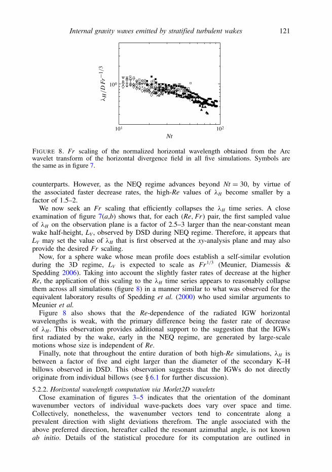
Now, for a sphere wake whose mean profile does establish a self-similar evolutionduring the 3D regime, LV is expected to scale as Fr1/3 (Meunier, Diamessis &Spedding 2006). Taking into account the slightly faster rates of decrease at the higherRe, the application of this scaling to the λH time series appears to reasonably collapsethem across all simulations (figure 8) in a manner similar to what was observed for theequivalent laboratory results of Spedding et al. (2000) who used similar arguments toMeunier et al.
Figure 8 also shows that the Re-dependence of the radiated IGW horizontalwavelengths is weak, with the primary difference being the faster rate of decreaseof λH . This observation provides additional support to the suggestion that the IGWsfirst radiated by the wake, early in the NEQ regime, are generated by large-scalemotions whose size is independent of Re.
Finally, note that throughout the entire duration of both high-Re simulations, λH isbetween a factor of five and eight larger than the diameter of the secondary K–Hbillows observed in DSD. This observation suggests that the IGWs do not directlyoriginate from individual billows (see § 6.1 for further discussion).
5.2.2. Horizontal wavelength computation via Morlet2D waveletsClose examination of figures 3–5 indicates that the orientation of the dominant
wavenumber vectors of individual wave-packets does vary over space and time.Collectively, nonetheless, the wavenumber vectors tend to concentrate along aprevalent direction with slight deviations therefrom. The angle associated with theabove preferred direction, hereafter called the resonant azimuthal angle, is not knownab initio. Details of the statistical procedure for its computation are outlined in
122 A. M. Abdilghanie and P. J. Diamessis
Nt
100
80
60
40
20
–5 50–10 10
(a) 100
80
60
40
20
–5 50–10 10
(b)
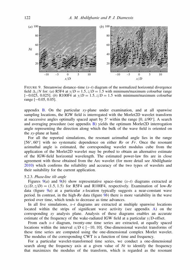
FIGURE 9. Streamwise distance–time (x–t) diagram of the normalized horizontal divergencefield 1z/N for: (a) R5F4 at y/D = 1.5, z/D = 1.5 with minimum/maximum colourbar range[−0.025, 0.025]; (b) R100F4 at y/D = 1.5, z/D = 1.5 with minimum/maximum colourbarrange [−0.05, 0.05].
appendix B. On the particular xy-plane under examination, and at all spanwisesampling locations, the IGW field is interrogated with the Morlet2D wavelet transformat successive angles optimally spaced apart by 5◦ within the range [0,±90◦]. A searchand averaging procedure (see appendix B) yields the optimum Morlet2D interrogationangle representing the direction along which the bulk of the wave field is oriented onthe xy-plane at hand.
For all the reported simulations, the resonant azimuthal angle lies in the range[56◦, 60◦] with no systematic dependence on either Re or Fr . Once the resonantazimuthal angle is estimated, the corresponding wavelet modulus cube from theapplication of the Morlet2D wavelet may be probed to obtain an alternative estimateof the IGW-field horizontal wavelength. The estimated power-law fits are in closeagreement with those obtained from the Arc wavelet (for more detail see Abdilghanie2010) which confirms the reliability and accuracy of the two types of wavelets andtheir suitability for the current application.
5.2.3. Phase-line tilt angleFigures 9(a) and 9(b) show representative space–time (x–t) diagrams extracted at
(y/D, z/D) = (1.5, 1.5) for R5F4 and R100F4, respectively. Examination of low-Redata (figure 9a) at a particular x-location typically suggests a near-constant waveperiod. In contrast, in the high-Re data (figure 9b) there is more variability in the waveperiod over time, which tends to decrease as time advances.
In all five simulations, x–t diagrams are extracted at multiple spanwise locationslocated within the strips of significant wave activity (see appendix A) on thecorresponding xy analysis plane. Analysis of these diagrams enables an accurateestimate of the frequency of the wake-radiated IGW field at a particular y/D-offset.
From each x–t diagram, twenty-one time series are extracted, at equally spacedlocations within the interval x/D ∈ [−10, 10]. One-dimensional wavelet transforms ofthese time series are computed using the one-dimensional complex Morlet wavelet.The modulus of the corresponding CWT is a function of time and frequency.
For a particular wavelet-transformed time series, we conduct a one-dimensionalsearch along the frequency axis at a given value of Nt to identify the frequencythat maximizes the modulus of the transform, which is regarded as the resonant

Internal gravity waves emitted by stratified turbulent wakes 123
20
30
40
50
40 60 80Nt
20 10010
60
FIGURE 10. Evolution of the phase-line-tilt/polar angle obtained from the one-dimensionalwavelet transforms. Symbols are the same as in figure 7.
frequency. Now, across the wavelet transforms for all time series, at a given Nt, theresonant frequencies are conditionally averaged. The conditional average retains onlyfrequencies with a corresponding transform modulus value above 50 % of the globalmaximum across all time series. The frequencies are finally mapped onto equivalentphase-line tilt angles θ through the IGW dispersion relation.
A better understanding of the spanwise dependence of the spanwise variability ofthe phase-line tilt angle, θ , of the emitted IGW field may be gained by examiningfigure 10 which shows the evolution of θ at two representative spanwise locationsfor each of the five simulations considered here. The evolution of θ (and associatedfrequency value for a particular simulation) is consistent with the qualitative featuresfound in figure 9(a,b). The observed values lie in the range θ ∈ [26◦, 50◦], which wasobserved in previous studies of IGWs generated in a well-mixed layer adjacent toa stable stratification (Sutherland & Linden 1998; Dohan & Sutherland 2003, 2005;Aguilar et al. 2006; Taylor & Sarkar 2007; Munroe & Sutherland 2008; Pham et al.2009).
In figure 10, at low Re, the phase-line tilt angles for all three Fr values is stronglyconcentrated around 31◦. Some weak departure to values no lower than θ = 26◦ occursat later times when wave radiation has significantly diminished. The value of θ = 31◦
is close to 35◦, the angle that maximizes the group velocity of the waves according tolinear theory (Sutherland 2010). Accordingly, waves propagating at such an angle willexperience the minimum viscous decay.
In the same figure, at high Re, the earliest observations of phase-line tilt angles, atNt = 20, lie within the range [40◦, 50◦]; the IGW energy propagates at angles that arecloser to the horizontal. Similar to the wavelengths, the computed phase-line-tilt anglesshow pronounced random spanwise variability relative to those at low Re. Now, thephase-line-tilt angles, especially around the time of maximum wave activity, are closeto 45◦, the value which maximizes the momentum extraction from the wake shearprofile (Sutherland 2010). Nevertheless, at later times, the high-Re time series of θconverge to values close to those of their low-Re counterparts.
5.3. Viscous effects in the propagation of radiated IGWsIt is of interest to assess the role of viscosity in the selection of particular frequencysubranges by the propagating IGW. We propose to track the distribution of resonant
124 A. M. Abdilghanie and P. J. Diamessis
0
1
2
3
4
0.4 0.6 0.8 1.0 1.2 1.40.2 1.6
0.250.500.75
0.00
1.00
(a) (b)
0
1
2
3
6
5
4
0.4 0.6 0.8 1.0 1.20.2
1.251.501.75
1.00
2.00
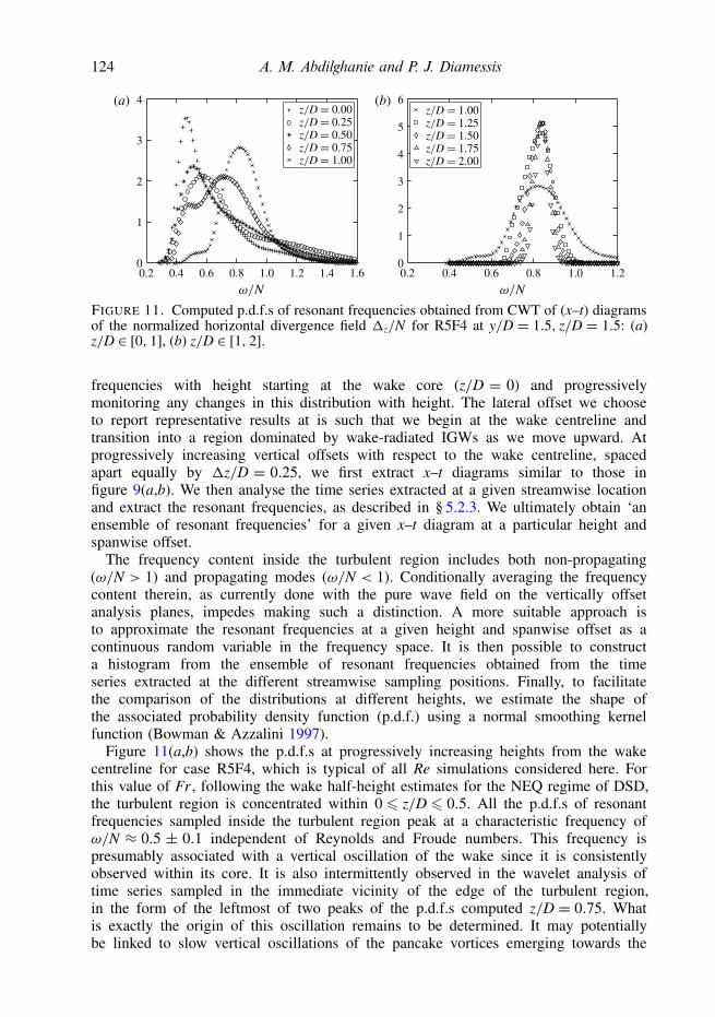
FIGURE 11. Computed p.d.f.s of resonant frequencies obtained from CWT of (x–t) diagramsof the normalized horizontal divergence field 1z/N for R5F4 at y/D = 1.5, z/D = 1.5: (a)z/D ∈ [0, 1], (b) z/D ∈ [1, 2].
frequencies with height starting at the wake core (z/D = 0) and progressivelymonitoring any changes in this distribution with height. The lateral offset we chooseto report representative results at is such that we begin at the wake centreline andtransition into a region dominated by wake-radiated IGWs as we move upward. Atprogressively increasing vertical offsets with respect to the wake centreline, spacedapart equally by 1z/D = 0.25, we first extract x–t diagrams similar to those infigure 9(a,b). We then analyse the time series extracted at a given streamwise locationand extract the resonant frequencies, as described in § 5.2.3. We ultimately obtain ‘anensemble of resonant frequencies’ for a given x–t diagram at a particular height andspanwise offset.
The frequency content inside the turbulent region includes both non-propagating(ω/N > 1) and propagating modes (ω/N < 1). Conditionally averaging the frequencycontent therein, as currently done with the pure wave field on the vertically offsetanalysis planes, impedes making such a distinction. A more suitable approach isto approximate the resonant frequencies at a given height and spanwise offset as acontinuous random variable in the frequency space. It is then possible to constructa histogram from the ensemble of resonant frequencies obtained from the timeseries extracted at the different streamwise sampling positions. Finally, to facilitatethe comparison of the distributions at different heights, we estimate the shape ofthe associated probability density function (p.d.f.) using a normal smoothing kernelfunction (Bowman & Azzalini 1997).
Figure 11(a,b) shows the p.d.f.s at progressively increasing heights from the wakecentreline for case R5F4, which is typical of all Re simulations considered here. Forthis value of Fr , following the wake half-height estimates for the NEQ regime of DSD,the turbulent region is concentrated within 0 6 z/D 6 0.5. All the p.d.f.s of resonantfrequencies sampled inside the turbulent region peak at a characteristic frequency ofω/N ≈ 0.5 ± 0.1 independent of Reynolds and Froude numbers. This frequency ispresumably associated with a vertical oscillation of the wake since it is consistentlyobserved within its core. It is also intermittently observed in the wavelet analysis oftime series sampled in the immediate vicinity of the edge of the turbulent region,in the form of the leftmost of two peaks of the p.d.f.s computed z/D = 0.75. Whatis exactly the origin of this oscillation remains to be determined. It may potentiallybe linked to slow vertical oscillations of the pancake vortices emerging towards the

Internal gravity waves emitted by stratified turbulent wakes 125
end of the NEQ regime (Geoffrey Spedding, personal communication). Note that theenergy density associated with the collapse of a well-mixed region in the experimentsof Wu (1969) was found to peak around ω/N ≈ 0.8. However, any connection of Wu’sfinding with those reported here is at best tenuous since the turbulent wake does notundergo a similar collapse process.
Figure 11(a) shows that all the p.d.f.s up to z/D = 0.5 have a single peak and areskewed to the right, towards ω/N > 1, with a visibly long tail. In all the simulationsconsidered here (not shown), the right tail of all computed p.d.f.s for ω/N > 1 insidethe core converges to zero with some intermittent oscillations associated with lowprobability values.
In figure 11(a), a transition from a unimodal to a bimodal p.d.f. distributionsubsequently occurs at z/D = 0.75, which corresponds to the edge of the wakecore. This transition is associated with intermittent wake oscillations at the previouslyidentified lower frequency peak of ω/N ≈ 0.5 ± 0.1 and IGW emission at a higherfrequency peak. This higher peak shifts to even higher values over a very short verticaldistance, a possible outcome of highly nonlinear processes around the intermittentedge of the turbulent wake, converging to ω/N ≈ 0.85. At higher vertical offsets(figure 11b), the low-frequency peak vanishes and the p.d.f.s show strong rates ofdecay for frequencies on each side of the now dominant higher-frequency peak. Forz/D = 1.25 and above, a narrow spectrum strongly peaking only at ω/N ≈ 0.85 isobserved with this peak frequency corresponding to a propagation angle of 31◦.
The continuous narrowing with height of the computed p.d.f.s around the higher-frequency peak can be attributed to the rapid viscous decay of the low- andhigh-frequency components of the radiated IGW field, in agreement with thefundamental mechanism underlying the viscous decay model of Taylor & Sarkar(2007). Nonetheless, the particular formulation of the viscous decay model consideredby Taylor & Sarkar is not directly applicable to the wake-radiated IGW fieldconsidered here because the model relies on statistical stationarity and linearity of theunderlying signal. The first condition is violated on account of the decaying turbulentsource as opposed to the forced turbulent Ekman layer in Taylor & Sarkar (2007) thatemits waves in a statistically stationary manner. In addition, the viscous decay modelpropagates an initial wave frequency spectrum from a prescribed spatial origin into theambient fluid. Taylor & Sarkar select as a spatial origin a location where the IGWenergy flux peaks and it is expected that most of the waves have been generated belowthis level. In the case of the wake, the most obvious choice of the spatial origin wouldbe the edge of the turbulent wake. However, the rapid transition from a unimodal toa bimodal and back to a unimodal, though of a different peak frequency, structureof p.d.f.s in the vicinity of the wake edge, around z/D = 0.75, in figure 11(a,b)suggests that intermittent wave–turbulence interaction and other nonlinear processesare responsible for this rapid change in wave properties with vertical offset from thewake core. As a result, the second condition of applicability of the viscous decaymodel is also violated around the edge of the turbulent wake.
Note that application of the linear viscous decay model to fields with moderate tostrong nonlinearity, namely higher Reynolds-number Ekman layers, has already beenshown by Taylor & Sarkar (2008) to cause non-negligible errors in its predictions,namely an overestimation of the amplitude of high-frequency content of the wavespectrum. Additionally, the wave energy spectrum around the edge of the Ekman layerin Taylor & Sarkar (2007) is a lot broader than that in the wake edge and no rapidchange of wave properties with height is reported in the former case. It appears thatthe localization of the turbulent wake in the spanwise direction in our simulation, as
126 A. M. Abdilghanie and P. J. Diamessis
0
1
2
3
4
0.4 0.6 0.8 1.0 1.2 1.40.2 1.6
0.250.500.75
0.00
1.00
(a) (b)
1
2
3
6
5
4
0.4 0.6 0.8 1.0 1.20 0.2
1.251.501.75
1.00
2.00
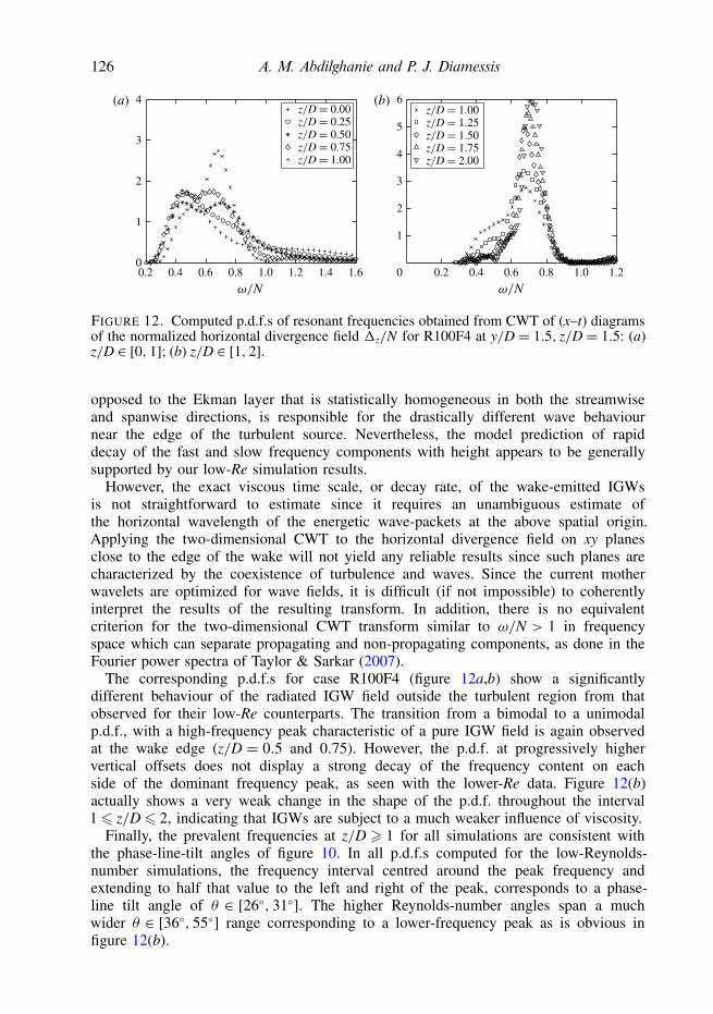
FIGURE 12. Computed p.d.f.s of resonant frequencies obtained from CWT of (x–t) diagramsof the normalized horizontal divergence field 1z/N for R100F4 at y/D = 1.5, z/D = 1.5: (a)z/D ∈ [0, 1]; (b) z/D ∈ [1, 2].
opposed to the Ekman layer that is statistically homogeneous in both the streamwiseand spanwise directions, is responsible for the drastically different wave behaviournear the edge of the turbulent source. Nevertheless, the model prediction of rapiddecay of the fast and slow frequency components with height appears to be generallysupported by our low-Re simulation results.
However, the exact viscous time scale, or decay rate, of the wake-emitted IGWsis not straightforward to estimate since it requires an unambiguous estimate ofthe horizontal wavelength of the energetic wave-packets at the above spatial origin.Applying the two-dimensional CWT to the horizontal divergence field on xy planesclose to the edge of the wake will not yield any reliable results since such planes arecharacterized by the coexistence of turbulence and waves. Since the current motherwavelets are optimized for wave fields, it is difficult (if not impossible) to coherentlyinterpret the results of the resulting transform. In addition, there is no equivalentcriterion for the two-dimensional CWT transform similar to ω/N > 1 in frequencyspace which can separate propagating and non-propagating components, as done in theFourier power spectra of Taylor & Sarkar (2007).
The corresponding p.d.f.s for case R100F4 (figure 12a,b) show a significantlydifferent behaviour of the radiated IGW field outside the turbulent region from thatobserved for their low-Re counterparts. The transition from a bimodal to a unimodalp.d.f., with a high-frequency peak characteristic of a pure IGW field is again observedat the wake edge (z/D = 0.5 and 0.75). However, the p.d.f. at progressively highervertical offsets does not display a strong decay of the frequency content on eachside of the dominant frequency peak, as seen with the lower-Re data. Figure 12(b)actually shows a very weak change in the shape of the p.d.f. throughout the interval16 z/D6 2, indicating that IGWs are subject to a much weaker influence of viscosity.
Finally, the prevalent frequencies at z/D > 1 for all simulations are consistent withthe phase-line-tilt angles of figure 10. In all p.d.f.s computed for the low-Reynolds-number simulations, the frequency interval centred around the peak frequency andextending to half that value to the left and right of the peak, corresponds to a phase-line tilt angle of θ ∈ [26◦, 31◦]. The higher Reynolds-number angles span a muchwider θ ∈ [36◦, 55◦] range corresponding to a lower-frequency peak as is obvious infigure 12(b).
Internal gravity waves emitted by stratified turbulent wakes 127
(a) (b)(× 10–4)
1
2
3
4
20 40 60 80
Nt0 100 20 40 60 80
Nt0 100
2
4
6
8
10
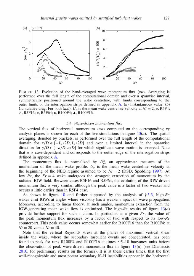
FIGURE 13. Evolution of the band-averaged wave momentum flux 〈uw〉. Averaging isperformed over the full length of the computational domain and over a spanwise interval,symmetrically positioned around the wake centreline, with limits corresponding to theouter limits of the interrogation strips defined in appendix A. (a) Instantaneous value. (b)Cumulative drag. For both (a,b), Uo is the mean wake centreline velocity at Nt = 2. ◦,R5F4;M,R5F16; �,R5F64; •,R100F4; N,R100F16.
5.4. Wave-driven momentum fluxThe vertical flux of horizontal momentum 〈uw〉 computed on the corresponding xyanalysis planes is shown for each of the five simulations in figure 13(a). The spatialaveraging, denoted by brackets, is performed over the full length of the computationaldomain for x/D ∈ [−Lx/2D,Lx/2D] and over a limited interval in the spanwisedirection for y/D ∈ [−a/D, a/D] for which significant wave motion is observed. Notethat a is case-dependent and corresponds to the outter edge of the interrogation stripsdefined in appendix A.
The momentum flux is normalized by U2o , an approximate measure of the
momentum of the mean wake profile. Uo is the mean wake centreline velocity atthe beginning of the NEQ regime assumed to be Nt = 2 (DSD; Spedding 1997). Atlow Re, the Fr = 4 wake undergoes the strongest extraction of momentum by theradiated IGW field. Between cases R5F16 and R5F64, the evolution of the IGW-drivenmomentum flux is very similar, although the peak value is a factor of two weaker andoccurs a little earlier than in R5F4 case.
As shown in figure 10 and further supported by the analysis of § 5.3, high-Rewakes emit IGWs at angles where viscosity has a weaker impact on wave propagation.Moreover, according to linear theory, at such angles, momentum extraction from theIGW-generating mean wake flow is optimized. The high-Re results of figure 13(a)provide further support for such a claim. In particular, at a given Fr , the value ofthe peak momentum flux increases by a factor of two with respect to its low-Recounterpart. This peak value occurs somewhat earlier for R100F16 than for R100F4: atNt = 20 versus Nt = 40.
Note that the vertical Reynolds stress at the planes of maximum vertical shearinside the wake, where the secondary turbulent events are concentrated, has beenfound to peak for runs R100F4 and R100F16 at times ∼5–10 buoyancy units beforethe observation of peak wave-driven momentum flux in figure 13(a) (see Diamessis2010, for preliminary results on the former). It is at these earlier times, that the firstwell-recognizable and most potent secondary K–H instabilities appear in the horizontal
128 A. M. Abdilghanie and P. J. Diamessis
vorticity field, establishing significant vertical transport corresponding to vertical eddyviscosities that are five times as large as their molecular counterpart. These verticaleddy viscosities are likely to become even larger at higher Re, given the Re/Fr2
scaling observed by DSD for buoyancy-driven shear which drives the secondary K–Hinstabilities. Nonetheless, the underlying cause of the occurrence of maximum verticaltransport of momentum by secondary turbulence and radiated IGWs at comparabletimes remains unclear and is a topic of future investigation.
Most importantly, due to prolonged IGW radiation, driven by the secondaryinstabilities and turbulence inside the wake core, significant values of the wave-drivenvertical momentum flux persist for as late as the end of the simulation for Fr = 4and up to Nt ≈ 60 for Fr = 16. This observation motivates the hypothesis that, withincreasing Re, the mean velocity profile of a stratified turbulent wake can lose anon-negligible portion of its initial momentum into emitted IGWs.
The above hypothesis may be quantitatively explored by following the procedureused by Sutherland & Linden (1998). Specifically, one integrates the vertical flux ofhorizontal momentum in time, under the assumption that this momentum is extractedfrom a turbulent source concentrated over a characteristic vertical length scale ofthe mean/background velocity profile which sustains the turbulence. In this case, theappropriate length scale is the wake half-height, LV , at the onset of the NEQ regime,which remains nearly constant throughout the NEQ regime (DSD; Spedding 2002).The relative reduction of the mean velocity profile, a measure of the wave-induceddrag, is then given by
1U
Uo= 2
UoLV
∫ Ntf
Nt=2〈uw〉 dt. (5.3)
The factor of two accounts for the momentum extracted by the sum of the upward anddownward propagating wave fields.
The evolution of the wave-induced drag is shown in figure 13(b). At a given Fr ,the high-Re wake undergoes a reduction in the strength of its mean velocity profilethat is nearly a factor of four higher than that of its low-Re counterpart. Note thatat Re = 5 × 10³, the two higher-Fr curves are barely distinguishable. Further work isneeded to determine whether such an observation indicates the possible existence of anRe-dependent upper bound of Fr , above which the mean momentum extracted by theradiated IGW field reaches a constant value. Our low-Re simulations have a maximumcumulative loss of momentum that is equal to 2 %, 1.4 % and 1 % of its initial valuefor Fr = 4, 16 and 64, respectively. The corresponding values for the high-Re runs are8.9 % and 6.2 %.
6. Discussion6.1. Length scales of IGWs and turbulence
Visual inspection of isopycnal contour plots (not shown here) indicates that the largest-scale turbulent overturning motions during the early stages of the NEQ regime havea vertical scale proportional to the full vertical extent of the wake. Therefore, sincethe IGWs arriving first at the xy analysis plane have a wavelength equal to 2.5 to 3times the wake half-height LV (see § 5.2.1), this initial wavelength is set by the abovelarge-scale overturns.
In § 5.2.1, the initial IGW horizontal wavelength, λH , is found to be equal to a smallmultiple of the mean wake half-height, LV . In addition, the λH time series collapseacross all cases when an Fr1/3 scaling is used. Recall that Gibson (1980) proposed that
Internal gravity waves emitted by stratified turbulent wakes 129
the IGWs first emitted by a localized turbulent event embedded in a linear stratificationhave a wavelength equal to the Ozmidov scale, LO, at the onset of buoyancy control(see § 1.2.3). Since we are using an implicit LES approach and a reliable estimate ofthe turbulent kinetic energy dissipation rate is not possible (see DSD for more details),we are unable to provide a corresponding reliable estimate of LO throughout the entirewake evolution. Nonetheless, we seek to, at least indirectly, assess Gibson’s claim byestablishing a connection between LO and LV .
The Ozmidov scale of a stratified turbulent event, as defined in (1.1), represents thelargest-scale vertical motion capable of generating density overturning (Ozmidov 1965;Dougherty 1961; Smyth & Moum 2000). At the onset of the NEQ regime, at Nt ≈ 2,visual examination of the isopycnal fields across all simulations (not shown) showsoverturning motions spanning a significant fraction of the vertical extent of the wake.As buoyancy indeed seizes control of the largest scales of turbulent motion at this time,it is reasonable to assume that the vertical scale of these overturns provides a measurefor LO at this time. As a result, it is very likely that LO = αLV at the beginning of theNEQ regime, with α ∈ [2, 4].
Moreover, Spedding (2002) proposed an Fr1/3 scaling for LO at the onset of theNEQ regime by assuming a self-similar power-law behaviour for the integral scale andcharacteristic velocity of the three-dimensional turbulence prior to the onset of thisregime. This scaling was independently confirmed by Spedding’s experimental datawhich indicated an Fr−7/3 scaling for the measured kinetic energy dissipation rate. Theabove observation-based estimate of LO and associated connection with LV at the onsetof the NEQ regime and the existence of anFr1/3 scaling for both LO and LV and alsoλH do lend support to Gibson’s claim. Additional support for this claim was providedby the recent experiments of Clarke & Sutherland (2010) who found that the Ozmidovscale of the turbulence in the vicinity of an oscillating cylinder, and not the cylinderdiameter, is what sets the wavelength of the radiated IGWs.
In the high-Re simulations considered here, turbulence persists throughout theentire NEQ regime. The question thus arises of whether the Ozmidov scale ofthe secondary events (occurring long after the original three-dimensional turbulencehas been overcome at all scales by buoyancy) sets the radiated IGW wavelengthobserved at later times during the NEQ regime. However, unlike the early-time three-dimensional turbulence that spans the large fraction of the wake’s full vertical extent,the secondary turbulence of the NEQ regime operates within the vertical confines ofthin horizontal vorticity layers (DSD; Brethouwer et al. 2007), with each secondaryturbulent event having its own local Ozmidov scale (Linborg 2006). An estimate of LO
during the NEQ regime at high Re may be obtained by examining stream-depth andspan-depth transects of the spanwise vorticity and isopycnal fields at the correspondingtimes (not shown here) and measuring the billow diameter. In such transects, thelargest overturning length scale is typically the diameter of the secondary K–H billows,which can then serve as an approximate measure of the desired value of LO (or upperbound thereof, depending on the degree of buoyancy control within the billow underconsideration). As discussed in § 5.2.1, the computed IGW horizontal wavelengths arealways a factor of 5 to 8 larger than the diameter of the K–H billows reported by DSD.Therefore, a more complex mechanism is operative at these later times at higher Re,whereby the secondary turbulent flow structures displace the isopycnal surfaces and theobserved values of λH come into being.
Finally, note that Taylor & Sarkar (2007) were not able to identify a correlationbetween λH and LO for a turbulent source operating in a well-mixed background.However, their observation is most likely linked to the considerably different turbulent

130 A. M. Abdilghanie and P. J. Diamessis
dynamics of their configuration compared to those of a wake embedded in a linearstratification.
6.2. Evolution of IGW wavelengthsDespite the link between the wavelength of the IGWs first emitted by the wake andthe vertical wake half-height at the beginning of the NEQ regime, questions remain asto what mechanism is responsible for the observed decrease over time of the computedwavelength. As proposed by BCH, IGW dispersion is the primary candidate here sincelong-wavelength components reach the analysis plane faster than waves with smallerwavelength. However, we find λH to decrease with power laws that are significantlyslower than the 1/Nt decrease rate which is characteristic of linear dispersion of wavesemitted by an isolated wave source.
Our estimated p.d.f.s of resonant frequencies in figures 11(a,b) and 12(a,b) alsoshow a very rapid change in wave properties near the edge of the turbulent wakeindicating that nonlinear processes including wave–wave interactions, interferenceof waves emitted from different locations within the wake, and wave–turbulenceinteractions are indeed important. Note that wave interference might be the causeof observed gradual loss of wavepacket coherence, especially at high Re (see figures 4and 5) where the density of waves and accordingly the number of effective localsources of IGWs within the wake noticeably increases.
At higher values of Re and Fr , since the wave steepness (and also the displacementamplitude; see § 5.1) increase significantly, nonlinear dispersion might act to addsignificant high-order corrections to wave frequency (Sutherland 2010). Finally, at highRe, the underlying physics becomes even more complicated, as the continuous IGWradiation is linked to different coherent vortical structures inside the wake such assuccessive secondary K–H instabilities and turbulence occurring throughout the NEQregime.
Further analysis, beyond the scope of this paper, would be needed to determine therole of the various mechanisms discussed above in setting the decrease rate of theIGW wavelength. From the point of view of developing more realistic reduced modelsof a stratified wake, the commonly employed models using impulsive sinks and sourcecould be augmented to contain multiple such sources of IGWs that interact nonlinearly,especially in the vicinity of the wake boundary, with nonlinear dispersion possiblyplaying an important role in IGW propagation.
6.3. IGW emission and momentum extraction at high Reynolds numberThe azimuthal angle of the wake-radiated IGWs is concentrated around a meandirection of approximately 60◦, independent of both Re and Fr . In contrast, the IGWphase-line-tilt angle with respect to the vertical does show a visible Re dependence(figure 10). In all low-Re simulations, the angles were constant over time and equalto θ = 31◦, a value which is close to the 35◦ value that maximizes the vertical groupvelocity of the wave field (Sutherland 2010). Further evidence of the dominant effectof viscosity at low Reynolds number is established through the gradual narrowingof the shape of resonant-frequency p.d.f.s with height along their propagation pathoutside the turbulent core, in agreement with the fast decay rate of low- and high-frequency components suggested by the viscous decay model of Taylor & Sarkar(2007). Waves with such a phase-line tilt angle are thus subject to minimum viscousdecay which suggests that, at these low Re, IGW radiation is a viscously-dominatedprocess, independent of the strength of the stratification.

Internal gravity waves emitted by stratified turbulent wakes 131
However, at high Re, the dynamics of the wake core and wave propagation aresubject to a much weaker influence of viscosity, thus allowing the resulting secondaryinstabilities and turbulence (DSD) within the wake to sustain IGW radiation at awider range of propagation angles. Taking into account any variability observed in thespanwise direction, the most intense wave emission now shifts towards phase-line tiltangles of θ ≈ 45◦ for a significant part of the NEQ regime. However, towards the endof this regime, the phase-line tilt angles asymptote towards the corresponding low-Reangle, indicating that, given enough time, viscous effects do become important. Wavespropagating at approximately 45◦ are associated with the maximum vertical flux ofhorizontal momentum (Sutherland 2010) away from the wake; the wake undergoes anon-negligible drag as indicated in figure 13(b). Consequently, whereas, at low Re,IGW emission has a negligible impact on the dynamics of the wake core, at highRe, especially at values of O(10) or higher than those considered in this paper, thenon-negligible wave drag it causes may considerably affect the wake dynamics.
It is interesting to note the propagation angle of θ ≈ 45◦ of emitted waves in theearlier part of the NEQ regime in our high-Re simulations and the prevalence of thissame angle value in the wave field emitted by forced turbulent mixed regions. In thelatter, Sutherland & Linden (1998) hypothesized that such an angle is the result of anequilibrium state of a highly nonlinear coupling between the emitted waves and themixed region dynamics. The presumed coupling maximizes wave drag on the meanshear within the turbulent region while, at the same time, prevents wave radiationfrom continuously draining the shear of its energy. The observed continuous decreaseof the wave emission angle over time in our high-Re simulations may be attributedto the drastically different manner in which buoyancy controls the dynamics of adecaying turbulent source in a stratified environment with respect to the dynamics of awell-mixed, forced turbulent source.
Insight into the coupling between the wake-radiated IGW field and the coherentvortical structures that generate it in a stratified fluid can be obtained by appealing tothe theoretical model of Plougonven & Zeitlin (2002). Nonetheless, a degree of cautionis warranted in this regard, as the above model is fully inviscid. The time at whichunambiguously identifiable pancake vortices emerge in the wake core corresponds tothe final stages of the NEQ regime, regardless of the wake Re (DSD). The bulkof IGW radiation has occurred prior to this point in time and is attributed to morecomplex flow structures (including secondary K–H instabilities and turbulence; see§ 1.2.1). Moreover, these quasi-horizontal vortical motions have a horizontal Reynoldsnumber (based on diameter and characteristic horizontal velocity) of O(1) that, byvirtue of viscosity, renders them robust to possible destabilization by IGW radiation,a phenomenon proposed by Plougoven & Zeitlin. Under more inviscid conditions,any destabilization of such vortices is also more likely to be caused by alternativemechanisms such as the zig-zag instability (Deloncle, Billant & Chomaz 2008).
Finally, a question that arises is whether, as Re is increased, there is an upper limitfor the efficiency at which IGW radiation can extract momentum, from the wake core.Moreover, as proposed by DSD, the duration of the NEQ regime increases with Re.The previous question may thus be reformulated as to whether, at operationally andgeophysically relevant Re of O(108) to O(1011) (Pao, Lai & Schemm 1982), IGWradiation depletes the wake of all its momentum and energy before viscous effects do(Gibson 1980).
Given that the K–H billows characteristic of the high-Re NEQ regime have ahorizontal length scale (DSD) considerably smaller than the horizontal wavelength
132 A. M. Abdilghanie and P. J. Diamessis
of the wake-emitted IGWs (see § 5.2.1), these waves are apparently generated bylarger scales of the turbulence inside the wake core; the K–H billows, nonetheless,should have a non-negligible role in the generation process. With respect to the spherediameter D, as one increases Re, these scales become increasingly removed from thesmaller scales of motion inside the wake which are directly impacted by viscosity.Given this reduced impact of viscosity, it is thus reasonable to assume that energyat these large-scales of the wake core is more readily available to be channelled toemitted IGWs than in the low-Re case. Moreover, one might perceive the radiationof IGWs as the dominant momentum/energy sink for the wake, as now buoyancy hasdominated almost the entire range of scales inside the wake. However, a competingprocess at high Re is the Kolmogorov-like forward cascade of turbulent energy inthe horizontal associated with the secondary instabilities and turbulence, as evidencedin the horizontal one-dimensional spectra with a broad inertial range (DSD; Riley &de Bruyn Kops 2003; Linborg 2006; Riley & Lindborg 2008) and the Kolmogorovscaling for the turbulent kinetic energy dissipation rate identified by (Brucker & Sarkar2010). Additional simulations at even higher Re, which will become feasible once theappropriate computational resources become available, will allow us to further explorethe above question on the relative strength of these two processes in depleting themean wake flow of its momentum, and energy.
7. Concluding remarks
The near-field properties of the internal gravity wave (IGW) field emitted by astratified turbulent wake with non-zero net momentum have been examined throughfully nonlinear spectral multidomain-based numerical simulations. Instrumental in theanalysis of the highly complex and spatially localized quasi-random wake-emittedIGW field is the use of the continuous wavelet transform (CWT) in one and twodimensions.
At higher Re, on account of the prolongation of the non-equilibrium (NEQ) regimein wake evolution through secondary Kelvin–Helmholtz instabilities and turbulence,IGW radiation persists much longer than at lower Re values typical of the laboratory,suggesting a possible change in IGW generation mechanism. A visible reductionin IGW horizontal wavelengths is observed at high Re. These wavelengths increasewith increasing Fr . Furthermore, the phase-line tilt angles of IGWs with respectto the vertical are found to lie in a narrow range of values that is predominantlyRe-dependent. At low Re, IGW emission is a viscously driven process, wherebywaves are radiated by the wake core at 31◦ from the vertical, an angle that allowsminimum viscous decay. The associated drag on the mean wake flow is negligible.At high Re, viscous effects are initially quite weaker, causing the radiated waves topropagate at angles within the range of [40◦, 55◦] which induce a non-negligible dragon the mean wake flow. Subsequently, viscous effects seem to drive the angle towardsits equivalent low-Re value. This particular result sets decaying stratified turbulentwakes apart from forced mixed turbulence where the higher wave propagation anglesare consistently observed regardless of Re. Additional work is needed to exploreSutherland’s hypothesis (Sutherland & Linden 1998) that nonlinear wave–mean flowinteractions are the direct cause of the predominance of such higher angles innumerical and experimental observations. Although IGW radiation can become asignificant sink of wake momentum and energy, further research is needed to ascertainwhether there is an upper bound on the rate of wake momentum and energy loss to
Internal gravity waves emitted by stratified turbulent wakes 133
emitted waves and how this rate compares to the turbulent kinetic energy dissipationrate inside the wake.
The quantification of the properties of the near-field wake-radiated IGWs enabledby this work provides insight that can contribute towards the refinement of existingreduced models of IGW radiation that are based on the superposition of impulsivemass sources and sinks (Voisin 1991, 1994). Critical to such a refinement effort isto take into account the significant reduction in decay rates of the IGW horizontalwavelengths and the continuous wave emission observed in the simulations. Thiscontinuous radiation may be contrasted to the pulse-like emission mechanism inherentin the above reduced models. In addition, the IGW fields generated in this study canserve as reliable initial conditions for computational fast-turnaround ray-tracing models(Broutman, Rottman & Eckert 2004).
Nevertheless, beyond the efforts presented here, significant additional work isneeded. On one hand, there are numerous aspects of the physics of IGW generationby a high-Re localized turbulent source that need to be clarified. In this regard, animportant unresolved question is to determine the exact differences in the dynamicsof a turbulent source operating in either a stratified environment or in a well-mixedbackground lying above or below a stratified region. On the other hand, additionalsimulations with more powerful computational resources are needed in the future.Runs in taller and wider domains would allow us to study conditions more relevantto geophysical and naval applications; that is a wider range of Re and Fr (Paoet al. 1982; Spedding 1997). In the latter case, Fr may be as high as O(500). Theavailability of such runs will enable further investigation into some of the issues andquestions raised in this study. These include the existence of an optimum Fr (andpossibly Re) value for maximizing momentum extraction by the waves, reliable scalingof the maximum displacement amplitude, and assessment of the potential for wavebreaking both near and far from the wake boundary.
Additionally, a more detailed computation of the energy flux transported by theemitted waves is needed. Computing this flux and assessing its relative strength withrespect to the turbulent kinetic energy dissipation rate and mixing induced within thewake would ideally require a highly costly DNS that would resolve the full rangeof scales within the wake core at high Re, namely the secondary turbulent events.Finally, an outstanding question of paramount importance lies in deciphering howexactly broadband turbulence embedded in a stably stratified background (and notneighbouring it while operating in a well-mixed region) generates IGWs and whetherthere is a particular coherent structure inside the wake core whose frequency orlength scale can be linked to the frequency or the wavelength of the radiated IGWs,respectively.
Acknowledgements
We are thankful to Professor G. R. Spedding for guidance on the theory and useof the two-dimensional continuous wavelet transforms. We also thank Professor J. J.Riley for a number of insightful comments. Q. Zhou is thanked for generating thethree-dimensional visualizations. We are grateful to three anonymous reviewers fortheir insightful commentary. Support through Office of Naval Research grant N00014-08-1-0235 administered by Dr R. Joslin is gratefully acknowledged. The second authoralso acknowledges the support of National Science Foundation CAREER award GrantOCE-0845558.
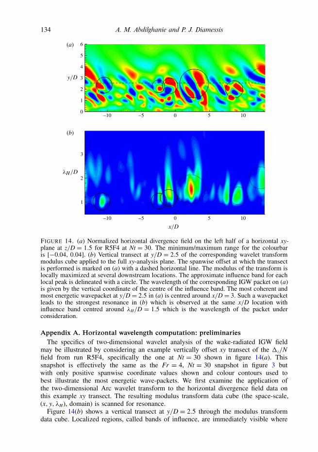
134 A. M. Abdilghanie and P. J. Diamessis
1
2
3
4
5
0
6
–10 –5 0 5 10
1
2
3
–10 –5 0 5 10
(b)
(a)
FIGURE 14. (a) Normalized horizontal divergence field on the left half of a horizontal xy-plane at z/D = 1.5 for R5F4 at Nt = 30. The minimum/maximum range for the colourbaris [−0.04, 0.04]. (b) Vertical transect at y/D = 2.5 of the corresponding wavelet transformmodulus cube applied to the full xy-analysis plane. The spanwise offset at which the transectis performed is marked on (a) with a dashed horizontal line. The modulus of the transform islocally maximized at several downstream locations. The approximate influence band for eachlocal peak is delineated with a circle. The wavelength of the corresponding IGW packet on (a)is given by the vertical coordinate of the centre of the influence band. The most coherent andmost energetic wavepacket at y/D= 2.5 in (a) is centred around x/D= 3. Such a wavepacketleads to the strongest resonance in (b) which is observed at the same x/D location withinfluence band centred around λH/D = 1.5 which is the wavelength of the packet underconsideration.
Appendix A. Horizontal wavelength computation: preliminariesThe specifics of two-dimensional wavelet analysis of the wake-radiated IGW field
may be illustrated by considering an example vertically offset xy transect of the 1z/Nfield from run R5F4, specifically the one at Nt = 30 shown in figure 14(a). Thissnapshot is effectively the same as the Fr = 4, Nt = 30 snapshot in figure 3 butwith only positive spanwise coordinate values shown and colour contours used tobest illustrate the most energetic wave-packets. We first examine the application ofthe two-dimensional Arc wavelet transform to the horizontal divergence field data onthis example xy transect. The resulting modulus transform data cube (the space-scale,(x, y, λH), domain) is scanned for resonance.
Figure 14(b) shows a vertical transect at y/D = 2.5 through the modulus transformdata cube. Localized regions, called bands of influence, are immediately visible where
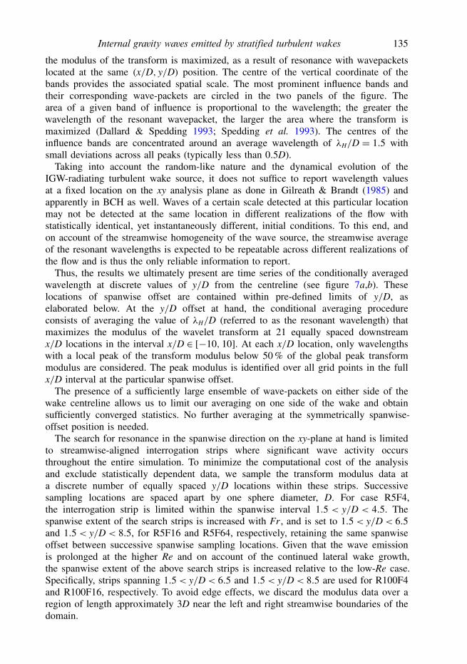
Internal gravity waves emitted by stratified turbulent wakes 135
the modulus of the transform is maximized, as a result of resonance with wavepacketslocated at the same (x/D, y/D) position. The centre of the vertical coordinate of thebands provides the associated spatial scale. The most prominent influence bands andtheir corresponding wave-packets are circled in the two panels of the figure. Thearea of a given band of influence is proportional to the wavelength; the greater thewavelength of the resonant wavepacket, the larger the area where the transform ismaximized (Dallard & Spedding 1993; Spedding et al. 1993). The centres of theinfluence bands are concentrated around an average wavelength of λH/D = 1.5 withsmall deviations across all peaks (typically less than 0.5D).
Taking into account the random-like nature and the dynamical evolution of theIGW-radiating turbulent wake source, it does not suffice to report wavelength valuesat a fixed location on the xy analysis plane as done in Gilreath & Brandt (1985) andapparently in BCH as well. Waves of a certain scale detected at this particular locationmay not be detected at the same location in different realizations of the flow withstatistically identical, yet instantaneously different, initial conditions. To this end, andon account of the streamwise homogeneity of the wave source, the streamwise averageof the resonant wavelengths is expected to be repeatable across different realizations ofthe flow and is thus the only reliable information to report.
Thus, the results we ultimately present are time series of the conditionally averagedwavelength at discrete values of y/D from the centreline (see figure 7a,b). Theselocations of spanwise offset are contained within pre-defined limits of y/D, aselaborated below. At the y/D offset at hand, the conditional averaging procedureconsists of averaging the value of λH/D (referred to as the resonant wavelength) thatmaximizes the modulus of the wavelet transform at 21 equally spaced downstreamx/D locations in the interval x/D ∈ [−10, 10]. At each x/D location, only wavelengthswith a local peak of the transform modulus below 50 % of the global peak transformmodulus are considered. The peak modulus is identified over all grid points in the fullx/D interval at the particular spanwise offset.
The presence of a sufficiently large ensemble of wave-packets on either side of thewake centreline allows us to limit our averaging on one side of the wake and obtainsufficiently converged statistics. No further averaging at the symmetrically spanwise-offset position is needed.
The search for resonance in the spanwise direction on the xy-plane at hand is limitedto streamwise-aligned interrogation strips where significant wave activity occursthroughout the entire simulation. To minimize the computational cost of the analysisand exclude statistically dependent data, we sample the transform modulus data ata discrete number of equally spaced y/D locations within these strips. Successivesampling locations are spaced apart by one sphere diameter, D. For case R5F4,the interrogation strip is limited within the spanwise interval 1.5 < y/D < 4.5. Thespanwise extent of the search strips is increased with Fr , and is set to 1.5< y/D< 6.5and 1.5< y/D< 8.5, for R5F16 and R5F64, respectively, retaining the same spanwiseoffset between successive spanwise sampling locations. Given that the wave emissionis prolonged at the higher Re and on account of the continued lateral wake growth,the spanwise extent of the above search strips is increased relative to the low-Re case.Specifically, strips spanning 1.5< y/D< 6.5 and 1.5< y/D< 8.5 are used for R100F4and R100F16, respectively. To avoid edge effects, we discard the modulus data over aregion of length approximately 3D near the left and right streamwise boundaries of thedomain.
136 A. M. Abdilghanie and P. J. Diamessis
Appendix B. Resonant azimuthal angle and circular data statisticsThis appendix outlines the technique used to compute the resonant azimuthal angle
of the wake-radiated IGW field. At increments of Nt = 1, the horizontal divergencefield on the xy-plane under consideration is transformed with the Morlet2D waveletusing selected a priori-prescribed interrogation angles in the interval [0,±90◦].Successive interrogation angles are equally spaced apart by 5◦. A smaller anglespacing is not only more costly, as more wavelet transforms are required, but is alsofound to not produce significantly different results between two successive angles. Foreach Nt value above, at a given y/D offset, the interrogation angles, φi, that resonatewith the wave field by producing the maximum modulus of the wavelet transform arerecorded at N = 21 equally spaced x/D locations within the interval x/D ∈ [−10, 10].
The computed resonant angles across all locations and times do not varysignificantly. Thus a single average angle, referred to as the resonant azimuthal angle,is ultimately reported, with the averaging performed over the range of φi given above.A standard circular data-averaging-technique (see Trauth 2010), is essential to avoidwhat is known as the wraparound effect at φ = 360◦. This effect incorrectly estimatesthe arithmetic average of the angles 6◦ and 354◦ as 180◦ and the standard deviationwith respect to the mean as 246◦. The appropriate average is defined as:
φ = tan−1(xr/yr), (B 1)
where
xr =N∑
i=1
sin(φi), (B 2)
and
yr =N∑
i=1
cos(φi). (B 3)
A measure of the dispersion around the average angle is then given by the circularvariance:
σo = 1− R, (B 4)
where
R=(√
x2r + y2
r
)/N. (B 5)
The more concentrated the angles are around a single mean direction, corresponding tothe resonant azimuthal angle, the smaller the value of the circular variance. In all thereported simulations, the mean directions of all resonance angles at all locations andtimes were in the range [56◦, 65◦] with typical circular variance σo ≈ 0.03 indicatingvery small departure from the mean direction. For a graphical illustration of theconcentration of the angles around a single mean value, the interested reader isreferred to the Rose diagrams in Abdilghanie (2010).
R E F E R E N C E S
ABDILGHANIE, A. M. 2010 A numerical investigation of turbulence-driven and forced generation ofinternal gravity waves in stratified mid-water. PhD thesis, Cornell University.
ADDISON, P. S. 2002 The Illustrated Wavelet Transform Handbook. Institute of Physics.

Internal gravity waves emitted by stratified turbulent wakes 137
AGUILAR, D. A. & SUTHERLAND, B. R. 2006 Internal wave generation from rough topography.Phys. Fluids 18, 066603.
AGUILAR, D. A., SUTHERLAND, B. R. & MURAKI, D. J. 2006 Laboratory generation of internalwaves from sinusoidal topography. Deep-Sea Res. II 53 (1–2), 96–115.
BONNETON, P., CHOMAZ, J. M. & HOPFINGER, E. J. 1993 Internal waves produced by theturbulent wake of a sphere moving horizontally in a stratified fluid. J. Fluid Mech. 254,23–40.
BONNIER, M., BONNETON, P. & EIFF, O. 1998 Far-wake of a sphere in a stably stratified fluid:characterization of vortex structures. Appl. Sci. Res. 59, 269–281.
BOWMAN, A. W. & AZZALINI, A. 1997 Applied Smoothing Techniques for Data Analysis: TheKernel Approach with S-Plus Illustrations, Oxford Statistical Science Series, vol. 18. OxfordUniversity Press.
BRETHOUWER, G., BILLANT, P., LINDBORG, E. & CHOMAZ, J. M. 2007 Scaling analysis andsimulation of strongly stratified turbulent flows. J. Fluid Mech. 585, 343–368.
BROUTMAN, D., ROTTMAN, J. W. & ECKERT, S. D. 2004 Ray methods for internal waves in theatmosphere and ocean. Annu. Rev. Fluid Mech. 36, 233–253.
BRUCKER, K. A. & SARKAR, S. 2010 A study of momentumless wakes in stratified fluids. J. FluidMech. 652, 373–404.
CHASHECHKIN, Y. D. 1989 Hydrodynamics of a sphere in a stratified fluid. Fluid Dyn. 24 (1), 1–7.CLARKE, H. A. & SUTHERLAND, B. R 2010 Generation, propagation, and breaking of an internal
wave beam. Phys. Fluids 22, 076601.DALLARD, T. & SPEDDING, G. R. 1993 2-D wavelet transforms: generalisation of the Hardy space
and application to experimental studies. Eur. J. Mech. (B/Fluids) 12 (1), 107–134.DELONCLE, A., BILLANT, P. & CHOMAZ, J. M. 2008 Nonlinear evolution of the zigzag instability
in stratified fluids: a shortcut on the route to dissipation. J. Fluid Mech. 599, 229–239.DIAMESSIS, P. J. 2010 Vertical transport in high Reynolds numbers stratified turbulent wakes. In
Sixth International Symposium on Environmental Hydraulics, Athens, Greece.DIAMESSIS, P. J., DOMARADZKI, J. A. & HESTHAVEN, J. S. 2005 A spectral multidomain penalty
method model for the simulation of high Reynolds number localized stratified turbulence.J. Comput. Phys. 202, 298–322.
DIAMESSIS, P. J., GURKA, R. & LIBERZON, A. 2010 Spatial characterization of vortical structuresand internal waves in a stratified turbulent wake using proper orthogonal decomposition. Phys.Fluids 22, 086601.
DIAMESSIS, P. J. & NOMURA, K. K. 2000 Interaction of vorticity, rate-of-strain and scalar gradientin stratified homogeneous sheared turbulence. Phys. Fluids 12, 1166–1188.
DIAMESSIS, P. J., SPEDDING, G. R. & DOMARADZKI, A. J. 2011 Similarity scaling and vorticitystructure in high Reynolds number stably stratified turbulent wakes. J. Fluid Mech. 671,52–95.
DOHAN, K. & SUTHERLAND, B. R. 2003 Internal waves generated from a turbulent mixed region.Phys. Fluids 15, 488.
DOHAN, K. & SUTHERLAND, B. R. 2005 Numerical and laboratory generation of internal wavesfrom turbulence. Dyn. Atmos. Oceans 40, 43–56.
DOMMERMUTH, D. G., ROTTMAN, J. W., INNIS, G. E. & NOVIKOV, E. A. 2002 Numericalsimulation of the wake of a towed sphere in a weakly stratified fluid. J. Fluid Mech. 473,83–101.
DOUGHERTY, J. P. 1961 The anisotropy of turbulence at the meteor level. J. Atmos. Terr. Phys. 21(2–3), 210–213.
DRUZHININ, O. A. 2009 Generation of internal waves by a turbulent jet in a stratified fluid. FluidDyn. 44, 213–223.
DURRAN, D. R. 1999 Numerical Methods for Wave Equations in Geophysical Fluid Dynamics.Springer.
GAYEN, B., TAYLOR, R. J. & SARKAR, S. 2010 Large eddy simulation of a stratified boundarylayer under an oscillatory current. J. Fluid Mech. 643, 233–266.
GIBSON, C. H. 1980 Fossil temperature, salinity and vorticity in the ocean. In Marine Turbulence(ed. J. C. T. Nihoul), pp. 221–258. Elsevier.
138 A. M. Abdilghanie and P. J. Diamessis
GILREATH, H. E. & BRANDT, A. 1985 Experiments on the generation of internal waves in astratified fluid. AIAA J. 23, 693–700.
GOURLAY, M. J., ARENDT, S. C., FRITTS, D. C. & WERNE, J. 2001 Numerical modelling ofinitially turbulent wakes with net momentum. Phys. Fluids 13, 3783–3802.
HOPFINGER, E. J., FLOR, J. B., CHOMAZ, J. M. & BONNETON, P. 1991 Internal waves generatedby a moving sphere and its wake in a stratified fluid. Exp. Fluids 11 (4), 255–261.
ISRAELI, M. & ORSZAG, S. A. 1981 Approximation of radiation boundary conditions. J. Comput.Phys. 41 (1), 115–135.
ITSWEIRE, E. C., KOSEFF, J. R., BRIGGS, D. A. & FERZIGER, J. H. 1993 Turbulence instratified shear flows: implications for interpreting shear-induced mixing in the ocean. J. Phys.Oceanogr. 23, 1508–1522.
KEELER, R. N., BONDUR, V. G. & GIBSON, C. H. 2005 Optical satellite imagery detection ofinternal wave effects from a submerged turbulent outfall in the stratified ocean. Geophys. Res.Lett. 32 (12), L12610.
KLEMP, J. B. & LILLY, D. K. 1978 Numerical simulation of hydrostatic mountain waves. J. Atmos.Sci. 35 (1), 78–107.
LIGHTHILL, J. 1978 Waves in Fluids. Cambridge University Press.LIGHTHILL, M. J. 1952 On sound generated aerodynamically. I. General theory. Proc. R. Soc. Lond.
A 211 (1107), 564–587.LILLY, D. K. 1983 Stratified turbulence and the mesoscale variability of the atmosphere. J. Atmos.
Sci. 40, 749–761.LINBORG, E. 2006 The energy cascade in a strongly stratified fluid. J. Fluid Mech. 550, 207–242.LINDEN, P. F. 1975 The deepening of a mixed layer in a stratified fluid. J. Fluid Mech. 71 (2),
385–405.MENG, J. C. S. & ROTTMAN, J. W. 1988 Linear internal waves generated by density and velocity
perturbations in a linearly stratified fluid. J. Fluid Mech. 186, 419–444.MEUNIER, P., DIAMESSIS, P. J. & SPEDDING, G. R. 2006 Self-preservation of stratified momentum
wakes. Phys. Fluids 18, 106601.MILES, J. W. 1971 Internal waves generated by a horizontally moving source. J. Geophys. Astrophys.
Fluid Dyn. 2 (1), 63–87.MOUM, J. N., HEBERT, D., PAULSON, C. A. & CALDWELL, D. R. 1992 Turbulence and internal
waves at the equator. Part I: Statistics from towed thermistors and a microstructure profiler.J. Phys. Oceanogr. 22 (11), 1330–1345.
MUNROE, J. R. & SUTHERLAND, B. R. 2008 Generation of internal waves by sheared turbulence:experiments. Environ. Fluid Mech. 8 (5), 527–534.
NAPPO, C. J. 2002 An Introduction to Atmospheric Gravity Waves. Academic.ORSZAG, S. A. & PAO, Y. H. 1975 Numerical computation of turbulent shear flows. Adv. Geophys.
18 (1), 225–236.OZMIDOV, R. V. 1965 On the turbulent exchange in a stably stratified ocean. Izv. Acad. Sci. USSR,
Atmos. Ocean. Phys. 1, 853–860.PAO, H. P., LAI, R. Y. & SCHEMM, C. E. 1982 Vortex trails in stratified fluids. Tech. Rep. 3(1).
Johns Hopkins Applied Physics Laboratory Technical Digest.PEAT, K. S. & STEVENSON, T. N. 1975 Internal waves around a body moving in a compressible
density-stratified fluid. J. Fluid Mech. 70 (4), 673–688.PHAM, H. T., SARKAR, S. & BRUCKER, K. A. 2009 Dynamics of a stratified shear layer above a
region of uniform stratification. J. Fluid Mech. 630, 191–223.PLOUGONVEN, R. & ZEITLIN, V. 2002 Internal gravity wave emission from a pancake vortex: an
example of wave–vortex interaction in strongly stratified flows. Phys. Fluids 14, 1259.RILEY, J. J. & DE BRUYN KOPS, S. M. 2003 Dynamics of turbulence strongly influenced by
buoyancy. Phys. Fluids 15, 2047–2059.RILEY, J. J. & LINDBORG, E. 2008 Stratified turbulence: a possible interpretation of some
geophysical turbulence measurements. J. Atmos. Sci. 65 (7), 2416–2424.RILEY, J. J. & METCALFE, R. W. 1987 Direct numerical simulations of turbulent patches in
stably-stratified fluids. In Stratified Flows I. Proceedings 3rd International Symp. on StratifiedFlows, California Institute of Technology, Pasadena.
Internal gravity waves emitted by stratified turbulent wakes 139
RILEY, J. J., METCALF, R. W. & WEISSMAN, M. A. 1981 Direct numerical simulations ofturbulence in homogeneously stratified fluids. In Non-linear Properties of Internal Waves,pp. 79–112. AIP.
ROBEY, H. F. 1997 The generation of internal waves by a towed sphere and its wake in athermocline. Phys. Fluids 9, 3353.
SMYTH, W. D. 1999 Dissipation-range geometry and scalar spectra in sheared stratified turbulence.J. Fluid Mech. 401, 209–242.
SMYTH, W. D. & MOUM, J. N. 2000 Length scales of turbulence in stably stratified mixing layers.Phys. Fluids 12, 1327.
SPEDDING, G. R. 1997 The evolution of initially turbulent bluff-body wakes at high internal Froudenumber. J. Fluid Mech. 337, 283–301.
SPEDDING, G. R. 2002 Vertical structure in stratified wakes with high initial Froude number.J. Fluid Mech. 454, 71–112.
SPEDDING, G. R., BROWAND, F. K., BELL, R. & CHEN, J. 2000 Internal waves from intermediate,or late-wake vortices. In Stratified Flows I – Fifth International Symposium (ed. R. Pieters,N. Yonemitsu & G.A. Lawrence), vol. 1, pp. 113–118. University of British Columbia,Vancouver.
SPEDDING, G. R., BROWAND, F. K. & FINCHAM, A. M. 1996 Turbulence, similarity scaling andvortex geometry in the wake of a towed sphere in a stably stratified fluid. J. Fluid Mech. 314,53–103.
SPEDDING, G. R., BROWAND, F. K., HUANG, N. E. & LONG, S. R. 1993 A 2-D complex waveletanalysis of an unsteady wind-generated surface wave field. Dyn. Atmos. Oceans 20 (1–2),55–77.
DE STATLER, M. B., SARKAR, S. & BRUCKER, K. A. 2010 Effect of the Prandtl number on astratified turbulent wake. Phys. Fluids 22, 095102.
SUTHERLAND, B. R. 2001 Finite-amplitude internal wavepacket dispersion and breaking. J. FluidMech. 429, 343–380.
SUTHERLAND, B. R. 2010 Internal Gravity Waves. Cambridge University Press.SUTHERLAND, B. R., FLYNN, M. R. & DOHAN, K. 2004 Internal wave excitation from a
collapsing mixed region. Deep-Sea Res. II 51, 2889–2904.SUTHERLAND, B. R. & LINDEN, P. F. 1998 Internal wave excitation from stratified flow over a thin
barrier. J. Fluid Mech. 377, 223–252.TAYLOR, J. R. & SARKAR, S. 2007 Internal gravity waves generated by a turbulent bottom Ekman
layer. J. Fluid Mech. 590, 331–354.TAYLOR, J. R. & SARKAR, S. 2008 Stratification effects in a bottom Ekman layer. J. Phys.
Oceanogr. 38 (11), 2535–2555.THORPE, S. A. 2005 The Turbulent Ocean. Cambridge University Press.TOWNSEND, A. A. 1965 Excitation of internal waves by a turbulent boundary layer. J. Fluid Mech.
22 (2), 241–252.TOWNSEND, A. A. 1968 Excitation of internal waves in a stably-stratified atmosphere with
considerable wind-shear. J. Fluid Mech. 32 (1), 145–171.TRAUTH, M. H. 2010 MATLAB R© Recipes for Earth Sciences. Springer.VOISIN, B. 1991 Internal wave generation in uniformly stratified fluids. Part 1. Green’s function and
point sources. J. Fluid Mech. 231, 439–480.VOISIN, B. 1994 Internal wave generation in uniformly stratified fluids. Part 2. Moving point sources.
J. Fluid Mech. 261, 333–374.WIJESEKERA, H. W. & DILLON, T. M. 1991 Internal waves and mixing in the upper equatorial
Pacific Ocean. J. Geophys. Res. 96 (C4), 7115–7125.WU, J. 1969 Mixed region collapse with internal wave generation in a density-stratified medium.
J. Fluid Mech. 35 (3), 531–544.ZAVOL’SKII, N. A. & ZAITSEV, A. A. 1984 Development of internal waves generated by a
concentrated pulse source in an infinite uniformly stratified fluid. J. Appl. Mech. Tech. Phys.25 (6), 862–867.