Embed Size (px)
Citation preview
J. Fluid Mech. (2012), vol. 692, pp. 369–394. c© Cambridge University Press 2012 369doi:10.1017/jfm.2011.519
Rotation of spheroidal particles in Couette flows
Haibo Huang1,2†‡, Xin Yang1, Manfred Krafczyk2 and Xi-Yun Lu1
1 Department of Modern Mechanics, University of Science and Technology of China, Hefei,Anhui 230026, China
2 Institute for Computational Modelling in Civil Engineering, Technische Universitat,Braunschweig 38106, Germany
(Received 15 November 2010; revised 1 October 2011; accepted 21 November 2011;first published online 5 January 2012)
The rotation of a neutrally buoyant spheroidal particle in a Couette flow is studied bya multi-relaxation-time (MRT) lattice Boltzmann method. We find several new periodicand steady rotation modes for a prolate spheroid for Reynolds numbers (Re) exceeding305. The simulations cover the regime up to Re6 700. The rotational behaviour of thespheroid appears to be not only sensitive to the Reynolds number but also to its initialorientation. We discuss the effects of initial orientation in detail. For 305 < Re < 345we find that the prolate spheroid reaches a periodic mode characterized by precessionand nutation around an inclined axis which is located close to the middle plane wherethe velocity is zero. For 345 < Re < 385, the prolate spheroid precesses around thevorticity direction with a nutation. For Re close to the critical Rec ≈ 345, a period-doubling phenomenon is observed. We also identify a motionless mode at higherReynolds numbers (Re > 445) for the prolate spheroid. For the oblate spheroid thedynamic equilibrium modes found are log rolling, inclined rolling and different steadystates for Re increasing from 0 to 520. The initial-orientation effects are studied bysimulations of 57 evenly distributed initial orientations for each Re investigated. Onlyone mode is found for the prolate spheroid for Re< 120 and 385< Re< 445. In otherRe regimes, more than one mode is possible and the final mode is sensitive to theinitial orientation. However, the oblate spheroid dynamics are insensitive to its initialorientation.
Key words: particle/fluid flows, suspensions
1. IntroductionSuspended particles in flows occur in many applications and play an important role
in industry. For example, the behaviour of suspended particles may affect the qualityof paper (Qi & Luo 2003). The rotational behaviour of prolate spheroids at very lowReynolds numbers (Re) has been studied theoretically for a long time. Jeffery (1922)investigated the motion of a single ellipsoid in shear flow while completely neglectinginertial effects. He concluded that the final rotational state of an ellipsoid cannotbe determined because it depends on initial conditions. To definitively determine thefinal rotational state, Jeffery (1922) hypothesized that ‘The particle will tend to adopt
† Email address for correspondence: [email protected]‡ Present address: Technische Universitat, Braunschweig 38106, Germany.

370 H. Huang, X. Yang, M. Krafczyk and X.-Y. Lu
that motion which, of all the motions possible under the approximated equations,corresponds to the least dissipation of energy’. Extensive analytical investigations(Harper & Chang 1968; Leal 1975) have studied the inertial effect at Re < 1 usingperturbation theory. However, their analyses are not applicable to large-Re cases. Leal(1980) have reviewed most of the previous relevant theoretical studies. There are alsosome relevant experimental works in the literature. Taylor (1923) confirmed Jeffery’shypothesis by investigating the orbit of a prolate or oblate spheroid in a Couette flowat a very low Reynolds number. However, Karnis, Goldsmith & Mason (1963) foundthat the inertial effect at Re = O(10−3) is sufficient to make non-spherical particlesadopt a motion that is different from Jeffery’s hypothesis.
Different numerical methods have also been used to study the motion of particlesin flows. Brady & Bossis (1988) adapted the Stokesian dynamics method forsimulating the motion of many particles in Stokes flow. However, this method isonly applicable to spherical particles and it neglects the inertial term, which mayhave a significant influence on the motion of particles. For finite-Reynolds-numberflows the Navier–Stokes equations have to be solved. Feng & Joseph (1995) simulatedthe motion of a single ellipse in two-dimensional (2D) creeping flows using a finite-element approach. They confirmed Jeffery’s hypothesis at Re ≈ 1. However, accordingto the investigation of the energy dissipation at Re = 0.1 and Re = 18, the numericalresults of Qi & Luo (2003) did not support Jeffery’s hypothesis. In this work wewill first validate our scheme for calculating relative viscosity and then re-evaluate thevalidity of the hypothesis.
Ding & Aidun (2000) used a lattice Boltzmann method (LBM), to simulate anelliptical cylinder in planar Couette flow and a single oblate spheroid for Re < 100 ina three-dimensional (3D) Couette flow. However, in the 3D simulation, the diameterof the oblate spheroid was fixed in the direction of the vorticity axis. They found thatbeyond a critical Reynolds number Rec = 81, the 3D oblate ellipsoid rotation wouldstop and the corresponding Rec for a 2D elliptical cylinder is ∼29. Later, experimentalresults of Zettner & Yoda (2001) confirmed the numerical finding for the 2D ellipticalcylinder.
Qi & Luo (2003) studied a prolate and an oblate particulate suspension in a 3DCouette flow for Re < 467 by LBM. They identified the following modes: tumbling,precessing and nutating, log rolling and inclined rolling for a prolate spheroid, whichare illustrated in figure 1(a,b,c,d) respectively. For an oblate spheroid, they identifiedthe log rolling and inclined rolling as Re increases. Yu, Phan-Thien & Tanner (2007)studied the problem for Re < 256 using a fictitious domain (FD) method, but thecritical transition Re was found to be very different to that of Qi & Luo (2003).Besides the modes mentioned above (Qi & Luo 2003), Yu et al. (2007) identified anextra mode for the oblate spheroid, i.e. the motionless mode. They also found that theorbital behaviour of the prolate spheroid is sensitive to the initial orientation. However,only up to two initial orientations of the spheroids were simulated in these studies.The prolate spheroid does not cease to rotate in their studies, which is not consistentwith the observations of Ding & Aidun (2000) and Zettner & Yoda (2001).
Here we investigate the rotation of a spheroid in a 3D Couette flow for Reynoldsnumbers up to 700. The numerical method used in our study is based on the LBM(Ladd 1994a,b; Aidun, Lu & Ding 1998; Ding & Aidun 2000). Using the LBM tostudy the motion of solid particles suspended in a fluid was first proposed by Ladd(1994a,b).
In the LBM approach used in Aidun et al. (1998) the non-slip boundarycondition on the particle–fluid interface is treated by the simple bounce-back rule

Rotation of spheroidal particles in Couette flows 371
x
z
y
x
z
y
x
z
y
x
y
z(a) (b)
(d) (e)
(c)
x
z
y
FIGURE 1. (Colour online available at journals.cambridge.org/flm) (a) Tumbling mode inthe flow-gradient plane (i.e. (y, z)-plane), (b) the precessing and nutating mode around thevorticity axis (i.e. x-axis), (c) the log-rolling mode, (d) the inclined rolling mode, and (e) theprecessing and nutating mode, around an inclined axis, which is represented by a thick-linearrow. The thin-line circles denote the particle rotating around its evolution axis (x′-axis). Thethick-line circles denote precession and nutation.
(He et al. 1997; Aidun et al. 1998). This treatment requires using a large numberof lattice nodes to accurately represent the geometrical boundaries of particles (Feng& Michaelides 2004). Recently, Bouzidi, Firdaouss & Lallemand (2001) proposed asecond-order-accurate treatment for moving boundaries based on an accurate curved-wall boundary treatment. In the present study, the fluid flow is solved by themulti-relaxation-time (MRT) LBM proposed by Lallemand & Luo (2003) while thetranslational and orientational motion of the spheroid is modelled by the Newtonianand Euler equations, respectively.
The present work is intended to provide a better understanding of the rotationalbehaviour of a non-spherical particle in shear flow. In § 2, the LBM and the basicequations for the motion of the solid particle are introduced briefly. The simulationresults for small Re are described in § 3. For this regime the results presented in thispaper agree well with the theoretical solution of Jeffery (1922) and numerical resultsobtained by other numerical methods (Yu et al. 2007). In §§ 4 and 5, the orientationaland rotational behaviours of a prolate and oblate spheroid at different Re are reported.The effects of initial orientation are also discussed. In § 6, the validity of Jeffery’shypothesis is examined. Conclusions are presented in § 7.
2. Numerical method2.1. MRT lattice Boltzmann equation
In our study, the fluid flow is solved by the MRT–LBM proposed by Lallemand &Luo (2003). The MRT lattice Boltzmann equation (LBE) is employed to solve theincompressible Navier–Stokes equations. The LBE is (d’Humieres et al. 2002)
|f (x+ eiδt, t + δt)〉 − |f (x, t)〉 = −M−1S[|m(x, t)〉 − |m(eq)(x, t)〉], (2.1)
372 H. Huang, X. Yang, M. Krafczyk and X.-Y. Lu
i 0 1 2 3 4 5 6 7 8 9 10 11 12 13 14 15 16 17 18
eix/c 0 1 −1 0 0 0 0 1 −1 1 −1 1 −1 1 −1 0 0 0 0eiy/c 0 0 0 1 −1 0 0 1 1 −1 −1 0 0 0 0 1 −1 1 −1eiz/c 0 0 0 0 0 1 −1 0 0 0 0 1 1 −1 −1 1 1 −1 −1
TABLE 1. Discrete velocities of the D3Q19 model.
where the Dirac notation of bra 〈·| and ket |·〉 vectors symbolize the row andcolumn vectors, respectively. The particle distribution function |f (x, t)〉 has 19components fi with i = 0, 1, 2, 3, . . . , 18 in our 3D simulations because the D3Q19velocity model is used. The collision matrix S = M · S · M−1 is diagonal withS = diag(s0, s1, . . . , s18), and|m(eq)〉 is the equilibrium value of the moment |m〉. Thematrix M illustrated in the Appendix is a linear transformation which is used to map avector |f 〉 in discrete velocity space to a vector |m〉 in moment space, i.e. |m〉 = M · |f 〉,|f 〉 = M−1 · |m〉.
In the above equation, ei are the discrete velocities of the D3Q19 model. The threecomponents eix, eiy, eiz are given in table 1, where c is the lattice speed defined asc= δx/δt. We use the lattice units of δx= 1 and δt = 1 in our study.
The macro-variables density ρ and momentum jζ are obtained from
ρ =∑
i
fi, jζ =∑
i
fieiζ , (2.2)
where ζ denotes the x, y, or z coordinates. Here the collision process is executed inmoment space (d’Humieres et al. 2002). The 19 moments |m〉 are (d’Humieres et al.2002)
|m〉 = (ρ, e, ε, jx, qx, jy, qy, jz, qz, 3pxx, 3πxx, pww, πww, pxy, pyz, pxz,mx,my,mz)T, (2.3)
where e, ε, and qζ are the energy, the energy squared, and the heat flux, respectively.(pxx, πxx, pww, πww, pxy, pyz, pxz) represent stresses and mx,my,mz are the third-ordermoments. The equilibria are given by (d’Humieres et al. 2002):
e(eq) =−11ρ + 19ρ0
jζ jζ , ε(eq) = wερ + wεj
ρ0jζ jζ , (2.4)
qeqζ =−
23
jζ , (2.5)
p(eq)xx =
13ρ0[2j2
x − (j2y + j2
z )], p(eq)ww =
1ρ0[j2
y − j2z ], (2.6)
p(eq)xy =
1ρ0
jxjy, p(eq)yz =
1ρ0
jyjz, p(eq)xz =
1ρ0
jxjz, (2.7)
π (eq)xx = wxxp
(eq)xx , π (eq)
ww = wxxp(eq)ww , (2.8)
m(eq)x = m(eq)
y = m(eq)z = 0, (2.9)
where ρ0 is the average density of the fluid, and wε , wεj, and wxx are free parameterswhich are set to wε = 3, wεj = −11/2, and wxx = −1/2 in our simulations. The
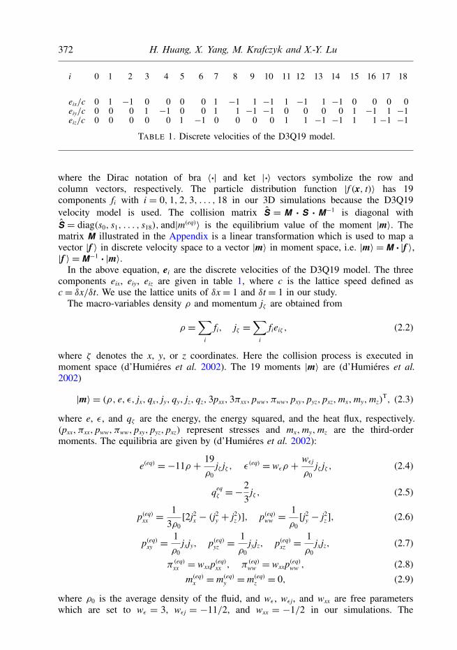
Rotation of spheroidal particles in Couette flows 373
z
y
x
U
U
O
M
FIGURE 2. (Colour online) Schematic diagram of a spheroid with its symmetry axis in thex′-direction in a Couette flow. Line OM represents the intersection of the (x, y) and the (x′, y′)coordinate planes. The two walls at y = 0 and y = Ny move in opposite directions. Periodicboundary conditions are applied in the x- and z-directions.
diagonal collision matrix S is given by (d’Humieres et al. 2002)
S ≡ diag(0, s1, s2, 0, s4, 0, s4, 0, s4, s9, s10, s9, s10, s13, s13, s13, s16, s16, s16). (2.10)
The parameters are chosen as: s1 = 1.19, s2 = s10 = 1.4, s4 = 1.2, s9 = 1/τ , s13 = s9,and s16 = 1.98. The parameter τ is related to the kinematic viscosity of the fluid withν = c2
s (τ − 0.5)δt and cs = c/√
3. The pressure in the flow field can be obtained fromthe density via the equation of state p= c2
sρ.
2.2. Kinematic equation of the particleThe translation of the solid particle is determined by solving Newton’s equation
mdU(t)
dt= F(t), (2.11)
where m is the mass of the suspended particle and F is the total force acting on theparticle.
The rotation of the spheroid is determined by the Euler equation, which is written as
I ·dΩ(t)
dt+Ω(t)× [I ·Ω(t)] = T(t), (2.12)
where I is the inertial tensor. Noted that in the body-fixed coordinate system(coordinates (x′, y′, z′) in figure 2), the tensor is diagonal and the principal momentsof inertia are Ix′x′ = m(b2 + c2)/5, Iy′y′ = m(a2 + c2)/5 and Iz′z′ = m(a2 + b2)/5, wherea, b and c are the lengths of three semi-principal axes of a spheroid in the x′-, y′-and z′-direction, respectively. Ω represents angular velocity and T are the torquesexerted on the solid particle in the same coordinate system. We note here that a simplefirst-order forward Euler integration procedure may not give accurate results.
It is not appropriate to solve the equation directly due to an inherent singularity(Qi 1999). Thus four quaternion parameters are used as generalized coordinates tosolve the corresponding system of equations. The quaternion parameters are definedas q0 = cos 1
2θ cos 12(φ + ψ), q1 = sin 1
2θ cos 12(φ − ψ), q2 = sin 1
2θ sin 12(φ − ψ), q3 =
cos 12θ sin 1
2(φ + ψ), where (φ, θ, ψ) are Euler angles. The coordinate transformation

374 H. Huang, X. Yang, M. Krafczyk and X.-Y. Lu
matrix from the space-fixed frame to the body-fixed frame can be written asq20 + q2
1 − q22 − q2
3 2(q1q2 + q0q3) 2(q1q3 − q0q2)
2(q1q2 − q0q3) q20 − q2
1 + q22 − q2
3 2(q2q3 + q0q1)
2(q1q3 + q0q2) 2(q2q3 − q0q1) q20 − q2
1 − q22 + q2
3
. (2.13)
With the quaternion formulation the angular velocity Ω in (2.12) can be solvedtogether with the following equation to obtain the transformation matrix (Qi 1999):
q0
q1
q2
q3
= 12
q0 −q1 −q2 −q3
q1 q0 −q3 q2
q2 q3 q0 −q1
q3 −q2 q1 q0
0Ωx′
Ωy′
Ωz′
. (2.14)
In this study, (2.12) and (2.14) are solved using a fourth-order-accurate Runge–Kuttaintegration procedure.
2.3. Fluid–solid couplingThe fluid–solid coupling in our study is based on the scheme of Lallemand & Luo(2003) and Aidun et al. (1998).
First we would like to introduce the curved-wall boundary condition briefly. In thestudy of Aidun et al. (1998), the wall is always assumed to be located at the middleof the link between a fluid node and a solid node. However, such an assumption wouldalter the curved-wall geometry on the grid level. It may also degrade the accuracyof the simulation at finite and higher Reynolds number (Mei et al. 2002). Here theaccurate moving-boundary treatment proposed by Lallemand & Luo (2003) is adopted.In the scheme the wall location at the link between a fluid node and a solid node isdetermined by the curved-wall geometry exactly. The fraction in the fluid region ofa grid space intersected by the boundary varies from zero to unity. The target of thescheme (Lallemand & Luo 2003) is to obtain fi(xb + ei, t) accurately, where fi is thedistribution function of the velocity ei ≡ −ei after streaming. xb is a solid boundarynode (SBN), which means a node inside the solid regime but it has at least one linkin direction ei connecting to a fluid node. The main idea of the treatment is usingLagrange interpolation to obtain unknown distribution functions and extrapolation isavoided to improve numerical stability (Bouzidi et al. 2001).
According to the studies of Mei et al. (2002) and Lallemand & Luo (2003), theforce on an SBN (xb) is calculated through the momentum exchange scheme (Meiet al. 2002):
F(b)(xb, t + 1
2
)=∑i
ei[fi(xb, t)+ fi(xb + ei, t)] × [1− w(xb + ei, t)], (2.15)
where w(x, t) is a scalar array. If the lattice site x is occupied by fluid at time t,w(x, t) = 0; if it is inside the solid body, w(x, t) = 1. Hence, in fact the summation isover all the links connecting to fluid nodes.
However, in the scheme of Lallemand & Luo (2003), they did not consider the forcedue to the fluid particle entering and leaving the solid region (Aidun et al. 1998). Herethis force contribution (Aidun et al. 1998) is involved.
At time step t, suppose a solid node becomes a fluid node, then the momentumof the solid node would convert to momentum of the fluid, and vice versa. The

Rotation of spheroidal particles in Couette flows 375
calculation of the forces due to momentum given to and taken from the particle isillustrated in the following.
An impulse force would be applied to the particle due to the momentum given tothe particle (a fluid node x becomes a solid particle). The force is given by (Aidunet al. 1998)
F(c)(x, t + 1
2
)=∑i
fi(x, t)ei. (2.16)
The momentum lost from the particle (a solid node x becomes a fluid node) iscalculated by (Aidun et al. 1998; Qi 1999)
ρ(x, t)u(x, t)= ρ(x, t)U(t)+Ω(t)× [x− X(t)], (2.17)
where U(t), X(t) are the velocity vector and position of the particle, respectively. Hereρ(x, t) is the density of the newly uncovered fluid node and can be assigned either asa locally averaged density (Aidun et al. 1998) or as the averaged density of the wholefluid ρ0 (Lallemand & Luo 2003). In our simulations, these schemes produce similarresults. The force due to the newly uncovered solid nodes is calculated by (Aidun et al.1998; Qi 1999)
F(u)(x, t + 12)=−ρ(x, t)u(x, t). (2.18)
To implement the collision and streaming procedure, the distribution functions fi ofa newly uncovered fluid node should be initialized. Two schemes are applicable. Thefi can be extrapolated through the nearby fluid node (Lallemand & Luo 2003) or theequilibrium distribution functions for fi can just be computed, i.e.
fi = f eqi = ωiρ
1+ eiζuζ
c2s
+ eiζuζeiδuδ2c4
s
− uζuζ2c2
s
(2.19)
(Lallemand & Luo 2003). Our study shows that the two schemes produce similarresults, which is consistent with the conclusion in the study of Lallemand & Luo(2003).
The total force on the solid particle at time t + 1/2 is given by (Aidun et al. 1998)
F(t + 1
2
)=∑SBN
F(b)(xb, t + 1
2
)+∑CN
F(c)(x, t + 1
2
)+∑UN
F(u)(x, t + 1
2
),
(2.20)
where CN and UN denote the covered nodes and the uncovered nodes, respectively.The torque on the solid particle can be calculated similarly to that in study of Aidunet al. (1998). The total force and torque at time t are averaged by those at time t − 1/2and t + 1/2 (Aidun et al. 1998).
2.4. Velocity boundary conditionFor the velocity boundary condition, the non-equilibrium extrapolation scheme is used(Guo, Zheng & Shi 2002). Extension of the scheme is illustrated below. In the scheme,the unknown post-collision moments |m+(xb, t)〉 of a node xb on the moving wall aredecomposed into two components: an equilibrium and a non-equilibrium part. Theequilibrium part is obtained from (2.4)–(2.9). In the equations, the velocity is specifiedand the density of a wall node ρ(xb) is obtained through extrapolation. It can besimply specified as ρ(xb)= ρ(x−b ); x−b denotes a fluid node very near to the wall node.For example, if the node indices for xb on the right wall are (i, jmax, k), the node
376 H. Huang, X. Yang, M. Krafczyk and X.-Y. Lu
indices for x−b are (i, jmax − 1, k). The unknown non-equilibrium part is also obtainedthrough extrapolation. Finally, for a node (xb) on the left or right moving walls (referto figure 2), the post-collision unknown moments |m+(xb, t)〉 are
|m+(xb, t)〉 = |m(eq)〉 + [|m+(x−b , t)〉 − |m(eq)(x−b , t)〉]. (2.21)
Note that the above equation should be implemented after the collision step for allinner fluid nodes has been implemented.
3. Validation of the numerical methodIn our study, the prolate or oblate spheroid is described by
x′2
a2+ y′2
b2+ z′2
c2= 1, (3.1)
where (x′, y′, z′) represents the body-fixed coordinate system. Euler angles (φ, θ, ψ)are used to describe the rotation of the particle. The spatial orientation of anybody-fixed frame (coordinate system) can be obtained by a composition of rotationsaround the (z′, x′, z′)-axis with the above Euler angles from an arbitrary frame ofreference (space-fixed frame). The composition of rotations is illustrated in figure 2and described below. Suppose that the body-fixed coordinates are initially overlappingwith the space-fixed coordinate system (x, y, z), and the symmetry axis of the spheroidis in the x′-direction. First the particle rotates around the z′-axis with a polar angleφ and then the particle rotates around the new x′-axis with an angle θ . Finally theparticle rotates around the z′-axis with an angle ψ . In the space-fixed coordinates, thestreamwise direction of the Couette flow is along the z-direction. The velocity gradientand the vorticity are oriented in the y- and x-direction, respectively. Two walls locatedat y = 0 and y = Ny move in opposite directions with speed U as shown in figure 2.Periodic boundary conditions are applied in both the x- and z-direction. The particleReynolds number is defined as
Re= 4Gd2
ν, (3.2)
where the shear rate is defined as G = 2U/Ny, d is the length of the semi-major axis(i.e. d = a for the prolate spheroid and d = b = c for the oblate spheroid) and ν is thekinematic viscosity.
In all of our numerical tests, the initial velocity field was initialized as a Couetteflow with a uniform pressure field (p0 = c2
sρ0). The particle is released at the centre ofthe computational domain with zero velocity. Although the translational motion of theparticle is not constrained, the spheroid centre is not found to depart from the centreof the computational domain in all simulated cases.
To validate our simulation, a case of an oblate spheroid rotating in a shear flow(Aidun et al. 1998) is simulated. In our simulation, the computational domain isNx × Ny × Nz = 40× 80× 110, and a, b, c of the oblate spheroid particle are 8, 16, 16,respectively. The initial orientation of the particle is (φ0, θ0, ψ0) = (90, 90, 90),which means that the evolution axis is parallel to the velocity direction of the twomoving walls. The results are illustrated in figure 3. From figure 3(a), we can see thatthe tumbling periods of Re = 50 and Re = 70 are different and the oblate spheroidwould stop when Re= 90. The transition of the critical Reynolds number Rec from thetumbling state to the stationary state is found ∼80. The tumbling period as a functionof Re predicted by the scaling law is T = C (Rec − Re)−1/2 (figure 3b), where Rec = 80

Rotation of spheroidal particles in Couette flows 377
0.9
0.7
0.5
0.3
Ang
ular
vel
ocity
(a) (b)
T
t
0.1
0 20 40 60 80 100Re
40 50 60 70 80–0.1
100
90
80
70
40
50
60
30
Re 50Re 70Re 90
FIGURE 3. (Colour online) (a) The angular velocity as a function of the non-dimensionaltime. (b) The tumbling period of the oblate spheroid as a function of Reynolds number. Thecircles are results of LBM simulations. The prediction (i.e., the solid line) of the scaling lawis T = C (Rec − Re)−1/2, where Rec = 80 and C ≈ 180, which agrees well with the simulatedresults.
and C ≈ 180, very consistent with that predicted by Aidun et al. (1998) with Rec = 81and C = 200.
To further validate our numerical method, LBM simulations are performed tocompare the analytical solution of the so-called Jeffery orbit (Jeffery 1922) and resultsobtained by another numerical method (Yu et al. 2007). In these simulations, themesh size is 96 × 96 × 96 and Re = 0.5. The confinement ratio is r1 = Ny/a = 8and the aspect ratio of the prolate spheroid (major diameter over minor diameter)is r2 = a/b = 2. The effect of the confinement ratio on the rotation of the spheroidwill be discussed at the end of § 4.1. In order to compare our results with Jeffery’sanalytical solution, the initial orientation is set as (φ0, θ0, ψ0) = (90, 0, 0), whichmakes the particle quickly enter a tumbling mode. Tumbling here implies a particlerotation about its minor axis and the minor axis is parallel to the vorticity direction.The criterion to identify a stable tumbling mode is (|T(n)− T(n− 1)|)/T(n) < 0.0005,where T(n) is the period of the nth cycle.
For a stable mode, the period does not change in time after some transient. Duringthe first two periods (t < 31.5) the tumbling mode already seems to have been reachedbecause (|T(2) − T(1)|)/T(2) = 0.000 35. We note for clarity that in all the LBMresults, the time and the angular velocity are non-dimensionalized by a scaling with1/G and G, respectively.
In figure 4(a) ωx is shown as function of time. The period obtained from LBM isT = 15.670 and that obtained from Jeffery’s analytical solution is T = 15.708. Thedeviation between the results of LBM and the analytical ones is ∼0.24 %. Hence, theLBM result at Re = 0.5 is very consistent with the analytical one. In figure 4(b) weshow directional cosine curves obtained by the LBM and the FD method (Yu et al.2007) during the first two periods. In this simulation, the particle’s initial orientation is(φ0, θ0, ψ0)= (0, 90, 45); α, β and γ here denote the angles between the x′-axis andthe space-fixed coordinates x-, y-, and z-axes, respectively (cos2α+ cos2β + cos2γ = 1).The result obtained by the LBM also agrees well with the numerical result obtainedby the FD method (Yu et al. 2007). It is noted that after a few periods, the rotationalmode for this case is also tumbling.
We also studied the confinement ratio effect on the rotation of the spheroid at lowRe. For r1 = 4 and identical Re, r2 and mesh resolution, the period obtained from

378 H. Huang, X. Yang, M. Krafczyk and X.-Y. Lu
0–2.0
–1.5
–1.0
–0.5
0
0.5
1.0
1.5
2.0
5 10 15
t20 25
LBMJeffery analytical solution
30 0 5 10 15
t
Dir
ectio
nal c
osin
es (
orie
ntat
ion)(a) (b)
20 25 30
0.2
0.4
0.6
0.8A
ngul
ar v
eloc
ity ,
x
FIGURE 4. (Colour online) Rotational and orientational behaviour of a prolate spheroid atRe = 0.5, r1 = 8 and r2 = 2: (a) angular velocity as a function of time obtained by LBMand Jeffery’s analytical solution, the initial orientation (φ0, θ0, ψ0) = (90, 0, 0); (b) thedirectional cosines as functions of time obtained by LBM simulation and the FD method (Yuet al. 2007) for (φ0, θ0, ψ0)= (0, 90, 45).
0 50 100 150 200
t250 300 350 0 10 20 30 40
t50 60
0.1
0.2
0.3
0.30
0.28
0.26
0.24
0.22
0.20
0.18
0.16
0.14
0.464 × 64 × 6496 × 96 × 96128 × 128 × 128
64 × 64 × 6496 × 96 × 96128 × 128 × 128
0.5(a) (b)
FIGURE 5. (Colour online) Grid independence study for the rotation of a prolate spheroidwith Re = 300 (a) and Re = 600 (b). In both cases, the initial orientation is (φ0, θ0, ψ0) =(5, 5, 5).
simulation is 2.6 % larger than the analytical one. Since the analytical solution is onlyapplicable to cases with large r1, if r1 is not large enough the two confined movingboundaries at y= 0 and y= Ny would slightly affect the period of rotation.
The mesh of the computational domain in all of our following simulations isNx × Ny × Nz = 96 × 96 × 96. To check whether this resolution is reasonable, a grid-convergence study was carried out for rotation of a prolate spheroid with Re = 300and 600. The directional cosines obtained by different meshes for the two cases areillustrated in figure 5. In all of the simulations, r1 = 4, r2 = 2 and U = 0.1 (in unitsdx/dt). In both cases, we can see that the results obtained by mesh 64× 64× 64 showa relatively large discrepancy with those obtained by 128 × 128 × 128. The resultsof mesh 96 × 96 × 96 are very close to those of mesh 128 × 128 × 128. Hence,in the Reynolds number range we studied (Re < 700), the mesh size 96 × 96 × 96seems sufficient to obtain accurate results. To investigate the compressibility effect of
Rotation of spheroidal particles in Couette flows 379
t
Ang
ular
vel
ocity
0 50 100 150 200t
0 50 100 150 200
0
0.2
0.4
0.6
(a) (b)
Dir
ectio
nal c
osin
es
–1.0
–0.5
0
0.5
1.0
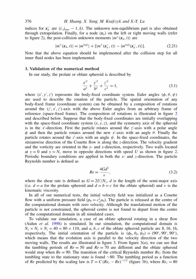
FIGURE 6. (Colour online) The rotational behaviour of the prolate spheroid at Re= 50. Theangular velocity ω = (ωx, ωy, ωz) (a) and orientation (b) as functions of time.
LBM with U = 0.1, we also simulated the case Re = 300 with U = 0.06, and foundno significant differences between the results for U = 0.1 and U = 0.06. Hence, thecompressibility effect is relatively small. In order to accelerate the computations wethus chose a velocity U = 0.1.
4. Rotation and orientation of a prolate spheroid4.1. Effects of Reynolds number
First, we study the effects of Reynolds number on the final mode of the prolatespheroid. In our numerical settings, the computational domain is 96 × 96 × 96 anda= 24, b= 12 and c= 12. The confinement ratio is Ny/a= 4 and the prolate spheroidaspect ratio is r2 = 2. The following results are based on the initial orientation(φ0, θ0, ψ0)= (5, 5, 5) implying a slight deviation of the particle’s axis of symmetrywith respect to the vorticity axis. Our results show that there are seven rotationaltransitions and eight steady or periodic modes in the range 0 < Re < 700. Weestimate the error of the critical Re separating these regimes to be ∼ ± 5 becausewe chose an increment of 1Re ≈ 10 in the simulations. For example, if two caseswith Re= 230 and Re= 240 have different rotational modes, Rec = 235 is assigned toseparate the different regimes. In order to identify the final mode we define a criterion(|T(n)−T(n−1)|)/T(n) < 0.0005, where T(n) denotes the period T of ωx(t) in the nthcycle. If ωx(t) does not change periodically, we used the following criterion to identifythe final steady mode (|ωx(t)− ωx(t − 1000)|)/ω(t) < 0.0005, where t is the time step.The different regimes labelled from (i) to (viii) are discussed below.
(i) Regime one (0< Re< 120).In this low-Reynolds-number range, the prolate spheroid reaches the tumbling mode.
The angular velocities ω = (ωx, ωy, ωz) as functions of time are shown in figure 6(a).We observe that in equilibrium ωx changes periodically in time while ωy and ωz arezero. To describe the tumbling mode in more detail, cosα, cosβ, cos γ as functionsof time are shown in figure 6(b). We observe that eventually cosα = 0 and cosβ andcos γ vary from −1 to 1, which means that the x′-axis is always perpendicular to thex-axis and the spheroid is rotating in the (y, z)-plane.
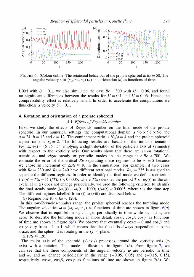
(ii) Re≈ 120.The major axis of the spheroid (x′-axis) precesses around the vorticity axis (x-
axis) with a nutation. This mode is illustrated in figure 1(b). From figure 7, wecan see that the three components of the angular velocity ω are periodic in timeand ωy and ωz change periodically in the range (−0.05, 0.05) and (−0.15, 0.15),respectively. cosα, cosβ, cos γ as functions of time are shown in figure 7(b). We
380 H. Huang, X. Yang, M. Krafczyk and X.-Y. Lu
t
Ang
ular
vel
ocity
0 50 100 150 200t
0 50 100 150 200
0
0.2
0.4
0.6(a) (b)
Dir
ectio
nal c
osin
es
–0.5
0
0.5
1.0
1.5
FIGURE 7. (Colour online) The precessing and nutating mode of the prolate spheroid atRe= 120. The angular velocity ω = (ωx, ωy, ωz) (a) and orientation (b) as functions of time.
Dir
ectio
nal c
osin
esD
irec
tiona
l cos
ines
0
0.5
1.0
0
0.2
0.4
0.6
0.8
Ang
ular
vel
ocity
Ang
ular
vel
ocity
0 100 200 300 400 0 100 200 300 400
0 100 200 300 400
0
0.2
0.4(a) (b)
(c) (d)
t0 100 200 300 400
t
0
0.1
0.2
0.3
0.4
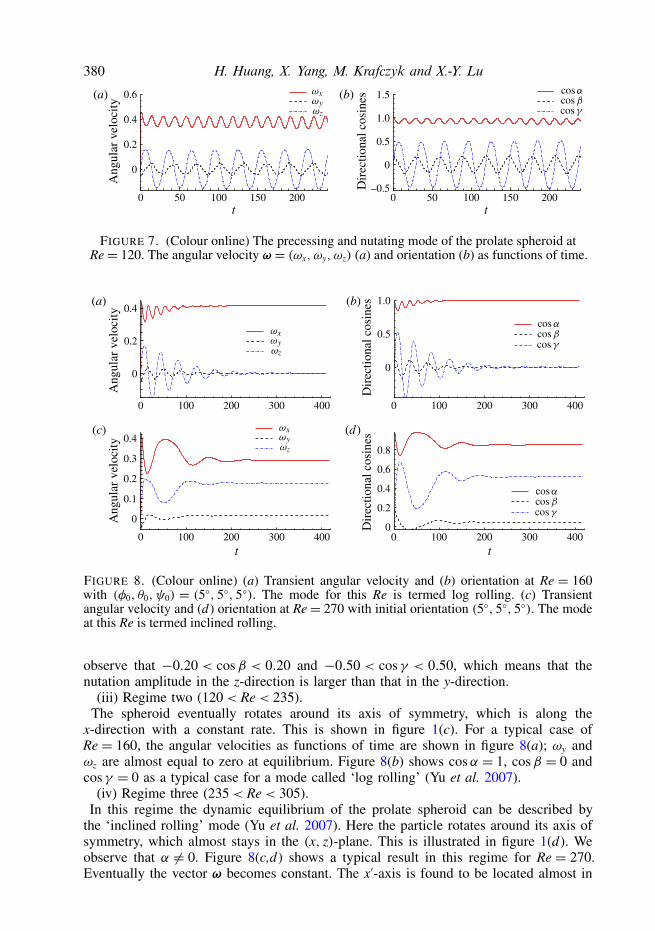
FIGURE 8. (Colour online) (a) Transient angular velocity and (b) orientation at Re = 160with (φ0, θ0, ψ0) = (5, 5, 5). The mode for this Re is termed log rolling. (c) Transientangular velocity and (d) orientation at Re= 270 with initial orientation (5, 5, 5). The modeat this Re is termed inclined rolling.
observe that −0.20 < cosβ < 0.20 and −0.50 < cos γ < 0.50, which means that thenutation amplitude in the z-direction is larger than that in the y-direction.
(iii) Regime two (120< Re< 235).The spheroid eventually rotates around its axis of symmetry, which is along the
x-direction with a constant rate. This is shown in figure 1(c). For a typical case ofRe = 160, the angular velocities as functions of time are shown in figure 8(a); ωy andωz are almost equal to zero at equilibrium. Figure 8(b) shows cosα = 1, cosβ = 0 andcos γ = 0 as a typical case for a mode called ‘log rolling’ (Yu et al. 2007).
(iv) Regime three (235< Re< 305).In this regime the dynamic equilibrium of the prolate spheroid can be described by
the ‘inclined rolling’ mode (Yu et al. 2007). Here the particle rotates around its axis ofsymmetry, which almost stays in the (x, z)-plane. This is illustrated in figure 1(d). Weobserve that α 6= 0. Figure 8(c,d) shows a typical result in this regime for Re = 270.Eventually the vector ω becomes constant. The x′-axis is found to be located almost in
Rotation of spheroidal particles in Couette flows 381
Dir
ectio
nal c
osin
esD
irec
tiona
l cos
ines
0 500 10000
0.2
0.4
0.6
0.8
1.0
0 500 1000 1500 2000–1.0
–0.5
0
0.5
1.0
t t0 500 1000 1500 2000
–0.2
0
0.2
0.4
Ang
ular
vel
ocity
Ang
ular
vel
ocity
0 500 1000
0
0.1
0.2
0.3
0.4(a) (b)
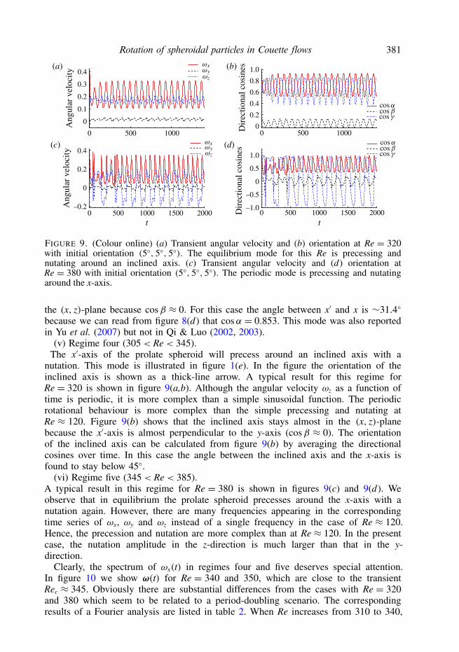
(c) (d)
FIGURE 9. (Colour online) (a) Transient angular velocity and (b) orientation at Re = 320with initial orientation (5, 5, 5). The equilibrium mode for this Re is precessing andnutating around an inclined axis. (c) Transient angular velocity and (d) orientation atRe = 380 with initial orientation (5, 5, 5). The periodic mode is precessing and nutatingaround the x-axis.
the (x, z)-plane because cosβ ≈ 0. For this case the angle between x′ and x is ∼31.4
because we can read from figure 8(d) that cosα = 0.853. This mode was also reportedin Yu et al. (2007) but not in Qi & Luo (2002, 2003).
(v) Regime four (305< Re< 345).The x′-axis of the prolate spheroid will precess around an inclined axis with a
nutation. This mode is illustrated in figure 1(e). In the figure the orientation of theinclined axis is shown as a thick-line arrow. A typical result for this regime forRe = 320 is shown in figure 9(a,b). Although the angular velocity ωz as a function oftime is periodic, it is more complex than a simple sinusoidal function. The periodicrotational behaviour is more complex than the simple precessing and nutating atRe ≈ 120. Figure 9(b) shows that the inclined axis stays almost in the (x, z)-planebecause the x′-axis is almost perpendicular to the y-axis (cosβ ≈ 0). The orientationof the inclined axis can be calculated from figure 9(b) by averaging the directionalcosines over time. In this case the angle between the inclined axis and the x-axis isfound to stay below 45.
(vi) Regime five (345< Re< 385).A typical result in this regime for Re = 380 is shown in figures 9(c) and 9(d). Weobserve that in equilibrium the prolate spheroid precesses around the x-axis with anutation again. However, there are many frequencies appearing in the correspondingtime series of ωx, ωy and ωz instead of a single frequency in the case of Re ≈ 120.Hence, the precession and nutation are more complex than at Re≈ 120. In the presentcase, the nutation amplitude in the z-direction is much larger than that in the y-direction.
Clearly, the spectrum of ωx(t) in regimes four and five deserves special attention.In figure 10 we show ω(t) for Re = 340 and 350, which are close to the transientRec ≈ 345. Obviously there are substantial differences from the cases with Re = 320and 380 which seem to be related to a period-doubling scenario. The correspondingresults of a Fourier analysis are listed in table 2. When Re increases from 310 to 340,

382 H. Huang, X. Yang, M. Krafczyk and X.-Y. Lu
Ang
ular
vel
ocity
1000 1500 2000
0
0.1
0.2
0.3
0.4(a) (b)
t t0 500 1000 1500 2000
–0.2
0
0.2
0.4
FIGURE 10. (Colour online) ω components as functions of time at Re= 340 (a) and 350 (b).
0 0.02 0.04 0.06 0.08 0.10
0.05
0.10
0.15
0 0.02 0.04 0.06 0.08 0.10
0.05
0.10
0.15
Am
plitu
de 0.20
0.25
0 0.02 0.04 0.06 0.08 0.10
0.05
0.10
0.15
0 0.02 0.04 0.06 0.08 0.10
0.05
0.10
0.15
Am
plitu
de
Frequency
(a) (b)
(c) (d)
Frequency
0.20
0.25
FIGURE 11. Frequency distribution and amplitude of ωx(t) at Re= 320 (a), 380 (b), 340 (c)and 350 (d).
Regime Re Main frequency (f0) Note
4 310 0.0147 —4 320 0.0136 —4 330 0.0127 —4 340 0.0113 f0/2 appears5 350 0.0124 f0/2 appears5 380 0.0122 —
TABLE 2. Main frequency of ωx for regimes four and five.
the main frequency of ωx(t) decreases monotonically from 0.0147 to 0.0113. For thetwo cases in regime five Re = 350 and 380, the main frequencies are almost identical.Figure 11 shows the detailed results of Fourier analysis using a Hamming windowfunction for ωx(t) at Re = 320, 380, 340, 350. It is found that at Re = 340 and 350in addition to the main frequency f0 a new independent frequency f0/2 appears. Thisindicates that the period-doubling phenomenon appears at Re= 340 and 350 comparedto Re= 320 and 380, respectively.

Rotation of spheroidal particles in Couette flows 383
Ang
ular
vel
ocity
Ang
ular
vel
ocity
0 50 100 150 200 250
0 50 100 150 200 250
0
0.2
0.4
0.6(a) (b)
(c) (d)
t
0 50 100 150 200 250
0 50 100 150 200 250t
0
0.1
0.2
0.3
0.4
Dir
ectio
nal c
osin
esD
irec
tiona
l cos
ines
–1.0
–0.5
0
0.5
1.0
0
0.5
1.0
FIGURE 12. (Colour online) (a) Transient angular velocity and (b) orientation at Re = 400with initial orientation (5, 5, 5). The rotational mode at this Re is tumbling. (c) Transientangular velocity and (d) orientation at Re= 500 with initial orientation (5, 5, 5). The modeat this Re is motionless.
(vii) Regime six (385< Re< 445).In this regime the tumbling mode reappears. Figure 12 shows the transient angular
velocity (a) and orientation (b) for Re = 400. Both amplitude and frequency of ωx arefound to be close to the low-Re cases depicted in figure 6.
(viii) Regime seven (445< Re< 700).Figures 12(c) and 12(d) show the transient angular velocity and orientation for
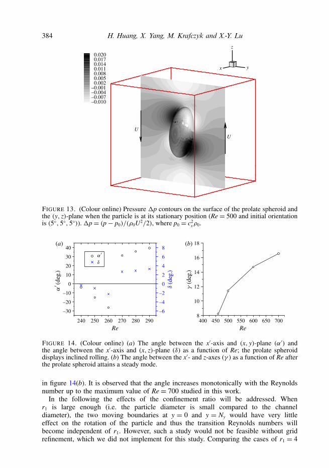
Re = 500, respectively. Eventually, the prolate spheroid motion stops and the axisof symmetry (i.e. x′-axis) stays almost in the (y, z)-plane. The angle between theevolution axis of the particle and the z-axis is ∼11 because cos γ = 0.98. Figure 13shows the pressure contours on the surface of the prolate spheroid and the (y, z)-planewhen the particle is at its stationary position. It is observed that the torques producedby the pressure and shear stress on its surface are in opposite directions. In this steadymode the two imposed torques are in balance because the sum of the torques is zero.Hence, the particle will not rotate any more and keeps its steady state position.
Having reported the rotational transitions, the effects of Re on the final orientationwill be addressed. In regime three, the angle between the x′-axis and (x, y)-plane (α′)and the angle between the x′-axis and (x, z)-plane (δ) as functions of Re are illustratedin figure 14(a). We can see that the evolution axis (x′-axis) is almost in the (x, z)-planebut may have a small deviation δ from it. Because δ is very small, the value of α′
is almost equal to α. α′ seems negative for lower Reynolds numbers but positive forhigher Reynolds numbers. Although the sign of α′ appears to be chosen randomly bythe flow system and the motion of the particle, the absolute values of the angles α′
and δ increase monotonically with Re but α′ is found not to exceed 45 for cases withr1 = 4 and r2 = 2.
For Re> 445, eventually the particle does not rotate any more and takes a stationaryposition in the flow field. The revolution axis of the spheroid (x′-axis) is on the(y, z)-plane because the deviations between the x′-axis and the plane are found to bebelow 0.5. The angle between the x′- and z-axis (γ ) as a function of Re is illustrated
384 H. Huang, X. Yang, M. Krafczyk and X.-Y. Lu
x y
z
0.0200.0170.0140.0110.0080.0050.002
–0.001–0.004–0.007–0.010
UU
FIGURE 13. (Colour online) Pressure 1p contours on the surface of the prolate spheroid andthe (y, z)-plane when the particle is at its stationary position (Re = 500 and initial orientationis (5, 5, 5)). 1p= (p− p0)/(ρ0U2/2), where p0 = c2
sρ0.
40 8
6
4
2
0
–2
–4
–6
30
20
10
0
–10
–20
–308
10
12
14
16
18
240 250 260 270
Re
(a) (b)
Re280 290 400 450 500 550 600 650 700
FIGURE 14. (Colour online) (a) The angle between the x′-axis and (x, y)-plane (α′) andthe angle between the x′-axis and (x, z)-plane (δ) as a function of Re; the prolate spheroiddisplays inclined rolling. (b) The angle between the x′- and z-axes (γ ) as a function of Re afterthe prolate spheroid attains a steady mode.
in figure 14(b). It is observed that the angle increases monotonically with the Reynoldsnumber up to the maximum value of Re= 700 studied in this work.
In the following the effects of the confinement ratio will be addressed. Whenr1 is large enough (i.e. the particle diameter is small compared to the channeldiameter), the two moving boundaries at y = 0 and y = Ny would have very littleeffect on the rotation of the particle and thus the transition Reynolds numbers willbecome independent of r1. However, such a study would not be feasible without gridrefinement, which we did not implement for this study. Comparing the cases of r1 = 4

Rotation of spheroidal particles in Couette flows 385
Regime Re range Case Possible final modes
1 0< Re< 120 Re= 50 Tumbling2 120< Re< 235 Re= 150 Log rolling; tumbling2 Re= 200 Log rolling; tumbling3 235< Re< 305 Re= 260 Inclined rolling; tumbling4 305< Re< 345 Re= 310 Precessing and nutating around an inclined
axis; tumbling5 345< Re< 385 Re= 350 Precessing and nutating around x-axis;
tumbling6 385< Re< 445 Re= 400 Tumbling7 445< Re< 700 Re= 500 Stationary; tumbling
TABLE 3. Typical modes of motion for the different regimes.
and 5 at typical Re in our study above, we found the rotation transitions at r1 = 5 aresimilar to those at r1 = 4. The critical Re at r1 = 5 are slightly different from thoseat r1 = 4. For example, for r1 = 5 the first transition Reynolds number is found to beRe ≈ 105 while Re is ∼120 for r1 = 4. Hence, for r1 = 4 the moving boundaries aty= 0 and y= Ny only have a minor effect on the rotation of a spheroid. For smaller r1,due to the significant effect of the moving boundaries, the rotational transitions may bevery different from the case of r1 = 4.
Hence, it should be kept in mind that the specific values of the critical Reynoldsnumbers separating the various regimes are r1-dependent, at least in the range ofconfinement ratio investigated here. A closer inspection of the velocity field indeedreveals that the wake of the particle may interact with that same particle due to the useof periodic boundary conditions (not shown here).
4.2. Effects of initial orientationIn this section we discuss the effects of initial orientation. For an initial orientationof (0, 0, 0) of the prolate spheroid, the rotational mode is always log rollingfor Re 6 700 whereas ωx increases for higher Re. When the x′-axis of the prolatespheroid is initially set in the (y, z)-plane, the particle reaches a tumbling mode for allRe< 700. In the following discussion we exclude these special initial orientations.
Table 3 shows typical modes of motion for the different Re regimes. Tumblingalways seems to be present even excluding the two special orientations mentionedabove.
For Re < 120 and 385 < Re < 445, the rotational mode would always be tumblingindependent of the initial orientation. For the other regimes the final mode depends onthe initial orientation. This conclusion holds for all modes of the 57 different initialorientations (shown in figure 16 below, except the special initial orientations (0, 0, 0)and x′ in the (y, z)-plane).
The initial orientation effect on the final mode at Re = 150 and 200 is displayedin figure 15. The sphere in the figure is used to guide the eye and a diameterdrawn on the sphere denotes a possible initial orientation. Each symbol on the spheredenotes an initial orientation of the minor and major axes of the oblate and prolateparticle, respectively. The grid intervals in the meridian and latitude directions areboth 22.5. The squares and discs represent the initial orientations which would resultin log-rolling and tumbling modes, respectively. In the cases of Re = 150 and 200,the regions which lead to log rolling on the surface of the spheres all look like
386 H. Huang, X. Yang, M. Krafczyk and X.-Y. Lu
x y
z
x y
z(b)(a)
FIGURE 15. (Colour online) Initial orientation effect on the final mode at Re = 150 (a) andRe = 200 (b). The squares () and circles () denote the initial orientations which eventuallyreach the log-rolling and tumbling modes, respectively.
x y
z
x y
z
x y
z
FIGURE 16. (Colour online) Initial orientation effect on the rotational mode at Re = 260for a prolate spheroid. The filled circles (•), open circles (), and squares () denote theinitial orientations which lead to inclined rolling with a positive cos γ (snapshot in upperinset), inclined rolling with a negative cos γ (snapshot in lower inset) and tumbling mode,respectively.
ellipses projected onto the surface. We also find that the squares and circles aresymmetric about the x-axis. That indicates that if two initial orientations are symmetricabout the x-axis, they will reach an identical mode. For example, at Re = 200, theinitial orientations (−22.5, 90,−22.5) and (22.5, 90, 22.5) eventually reach thesame mode – log rolling – while the initial orientations (−22.5, 90, 22.5) and(22.5, 90,−22.5) both display the tumbling mode. For two cases with initial

Rotation of spheroidal particles in Couette flows 387
orientations symmetric about the x-axis, the forces and torques acting on particles arealso symmetric about the x-axis due to the x-axis-symmetry of Couette flow. Hence, itis reasonable to expect that the two cases will follow two symmetric orbits and finallyreach an identical mode.
Comparing figures 15(a) and 15(b), we also find that the area occupied by squaresseems to increase from Re = 150 to Re = 200. Hence, for a random initial orientation,the log rolling mode may have more opportunities to appear at higher Re.
In regime three, figure 16 shows the initial orientations that lead to two differentmodes: inclined rolling and tumbling at Re = 260. For the inclined rolling mode, twosymmetric final orientations are possible. Snapshots of two final orientations with apositive cos γ and a negative cos γ are also illustrated on the upper and lower insets offigure 16, respectively. The sign of cos γ is thus determined by the initial orientation.From the distribution of the filled circles (•) and open circles () in figure 16, wefind that when one orientation is labelled , its x-axis-symmetric counterpart must belabelled • and vice versa. Hence, if the two initial orientations are symmetric about thex-axis, the final orientation of the inclined rolling mode is also symmetric about thex-axis which is due to the x-axis symmetry of the Couette flow.
We conclude that for Re = 150, 200, and 260 the final state will be the tumblingmode when initially x′ deviates far from the x-axis, i.e. the orientation closer tothe (y, z)-plane which perpendicular to the vorticity axis. A similar situation is alsoobserved at Re = 310, 350, 500. On the other hand, if initially x′ is close to thex-axis, the periodic and motionless mode would appear at Re = 310, 350 and 500,respectively.
5. Rotation and orientation of an oblate spheroid5.1. Effects of Reynolds number
We also carried out simulations for an oblate spheroid with Re from 0 to 520. In ournumerical settings, the computational domain is 96× 96× 96 and a= 12, b= 24, andc= 24. The confinement ratio is Ny/b= 4 and the aspect ratio r2 = b/a= 2. Here x′ isthe revolution axis or the axis of symmetry. Similar criteria as illustrated in § 4.1 wereused to identify the final mode. The critical Re to separate different regimes may havean error of ±4.
First we studied the effects due to varying Re. Cases with different Re but identicalinitial orientation (φ0, θ0, ψ0) = (5, 5, 5) were simulated. The final modes of theoblate spheroid are found to be simpler than those of the prolate spheroid. In thelow-Reynolds-number range (0 < Re < 112), the oblate spheroid will eventually spinat a constant rate around the revolution axis, which is parallel to the x-axis (α = 0).This mode is called ‘spinning’ (Qi & Luo 2003) or ‘log rolling’ (Yu et al. 2007). Inan intermediate-Reynolds-number range (112 < Re < 168), the spheroid will still spinaround the x′-axis. However, the revolution axis does not align with the vorticity axis(i.e. x-axis) again. It stays very close to the (x, y)-plane with α 6= 0. This mode iscalled ‘inclined rolling’ in the study of Yu et al. (2007). The angle α as a functionof Re is illustrated in figure 17(a). It increases from ∼10 to 70 for 120 < Re < 156.Furthermore, we can also see that the angle between the x′-axis and (x, y)-plane (δ) isalso increasing with Re although the angle amplitude is small for all cases studied.
In the higher-Reynolds-number range (168< Re< 520), the spheroid will eventuallystop rotating and the x′-axis will stay almost in the (y, z)-plane because the anglebetween x′-axis and the (y, z)-plane is less than 0.25 in this Reynolds number regime.The final angle β as a function of Re is illustrated in figure 17(b). It is observed that

388 H. Huang, X. Yang, M. Krafczyk and X.-Y. Lu
80 26
24
22
20
18
16
0
–2
–4
–6
–8
–10
70
60
50
40
30
20
10
115 125 135 145 200 250 300 350 400 450 500 550
Re Re155
z
x y
N
o
x
(a) (b)
FIGURE 17. (Colour online) (a) The angle between x′- and x-axes (α) and the angle betweenthe x′-axis and (x, y)-plane (δ) as a function of Re; an oblate spheroid displays inclined rolling.(b) The angle between the x′- and y-axes (β) as a function of Re, when the oblate spheroidtakes a stationary position. The inset shows the stationary position and β at Re = 350. LineON is a semi-principal axis of the oblate spheroid which is perpendicular to the x-axis. Inthese simulations, the initial orientations are (5, 5, 5).
the value of β is increasing with Re. At the stationary position, there is a balancebetween the torques of the viscous force and pressure exerted on the spheroid. Ourresults also show that the values of torques produced by the shear force and pressureincrease equally with Re. Our observation is consistent with the results of Yu et al.(2007) with a small discrepancy in Re because r1 = 5 in their study but a value ofr1 = 4 is used in the present study.
In the study of Qi & Luo (2003) it was anticipated that the oblate spheroid wasrotating about its major diameter which is parallel to the vorticity axis at Re> 400 fora random initial orientation. However, we did not observe this phenomenon. Althoughthis tumbling mode is found in our simulations, it is limited to very special caseswhere x′ is initially in the (y, z)-plane.
5.2. Effects of initial orientationFor the oblate spheroid, when the initial orientation is (0, 0, 0), the final mode isalways log rolling at all Re studied. We observe that those simulations where x′ isset perpendicular to the vorticity direction initially would eventually reach a tumblingmode at any Re < 520. In the following discussion we exclude these special initialorientations.
For Re = 100, we observed solely the log-rolling mode for all the 57 initialorientations depicted in figure 18.
At an intermediate Reynolds number Re = 140, we investigated the final modesensitivity to the initial orientation. A total of 57 cases with different initialorientations were simulated and the results are shown in figure 18. Except for thespecial cases mentioned above, only the inclined rolling mode exists at this Re.Figure 18 shows that the inclined x′-axis may be of a positive or a negative cosβ,which depends on the initial orientations. In this figure, the open circles (), filledcircles (•) and squares () denote the initial orientations which finally reach theinclined rolling with a negative cosβ and a positive cosβ and tumbling, respectively.Comparing two nodes symmetric about the x-axis, we find if one orientation islabelled , its x-axis-symmetric orientation must be labelled • and vice versa. Hence,

Rotation of spheroidal particles in Couette flows 389
y
z
x
x y
z
x y
z
FIGURE 18. (Colour online) Initial-orientation effect on the final mode at Re = 140 for anoblate spheroid. The open circles (), filled circles (•), and squares () denote the initialorientations which finally lead to inclined rolling with a negative cosβ (snapshot in the lowerinset), inclined rolling with a positive cosβ (snapshot in the upper inset) and tumbling mode,respectively.
if the two initial orientations are symmetric about the x-axis, the final orientations arealso symmetric about the x-axis.
For Re > 168 the particle will finally stop moving irrespective of its initialorientations. Thus for the oblate spheroid, the final mode appears to be insensitiveto the initial orientation.
The above regime classification, modes, and effects of initial orientation for bothprolate and oblate spheroids have been obtained numerically; they need to be verifiedin detail experimentally.
6. Energy dissipationAs mentioned in the introduction, Taylor (1923) and Feng & Joseph (1995)
confirmed Jeffery’s hypothesis experimentally and numerically for very small Reynoldsnumbers. Qi & Luo (2003) obtained some numerical results which are not consistentwith Jeffery’s hypothesis when they investigated the energy dissipation of a prolatespheroid in a Couette flow with Re= 0.1 and Re= 18.
Here we also investigated the energy dissipation represented by the relative viscosityπ of the flow system (Qi & Luo 2003), which is given by
π = ηs
ηf= 〈σ 〉ρνG
, (6.1)
where ηs and ηf are the effective suspension viscosity and solvent viscosity and〈σ 〉 is the average shear stress. However, Qi & Luo (2003) did not mention how

390 H. Huang, X. Yang, M. Krafczyk and X.-Y. Lu
they obtained 〈σ 〉. There are two conjectures. One may calculate 〈σ 〉 either throughaveraging the shear stress over both time and the entire spheroid surface, or throughaveraging the shear stress acting on the moving flat wall over time directly. They arereferred to as scheme 1 and scheme 2.
As we know, the shear stress in a fluid node can be obtained through σ =ρν(∂yw + ∂zv), where v and w are the velocity components in the y- and z-directions,respectively. We note that in the MRT–LBM, the second-order moments of thedistribution function are given by pyz =
∑ieiyeizfi = ρvw− τc2
sρ(∂yw+ ∂zv). Therefore,at each fluid node the shear stress is obtained through
σ = ρν (∂yw+ ∂zv)= ν
τc2s
(ρvw− pyz). (6.2)
In the lattice Bhatnagar–Gross–Krook (BGK) method, at each fluid node the shearstress can be obtained by σ = ρν(∂yw + ∂zv) = −(1 − (1/2τ))
∑f neqi eiyeiz, where
f neqi = fi − f eq
i .To calculate 〈σ 〉, a third option is a strictly volumetric average of (6.2), which
should be equivalent to scheme 2. In the following simulations, we found scheme 1 iswrong. Hence we mainly discuss scheme 2. In scheme 2, through integration the shearstress on the moving flat wall, we obtained the drag force acting on the flat wall. Theshear stress acting on a moving wall node is equal to that acting on the fluid node thatis nearest to the wall node. Then the spatial-averaged shear stress is equal to the dragforce divided by area of the moving flat wall. After the shear stress is further averagedby time, 〈σ 〉 is obtained.
To validate scheme 2, suspensions of spherical particles in a shear flow weresimulated. The numerical results were compared with Einstein’s theory on a dilutesuspension of spheres (Einstein 1905). According to Einstein’s theory, the relativeviscosity in dilute suspensions of spheres is (Einstein 1905) π = 1 + φ[η], where φ isthe solid volume fraction, and [η] = 5
2 is the intrinsic viscosity.In our simulations, mesh size is 100 × 100 × 100, τ = 1.0 and Re is fixed to be
0.5. Two cases with radii of a spherical particle r = 15 and 17 were simulated, withsolid volume fractions 1.41 % and 2.06 %, respectively. They can be regarded as dilutesuspensions. According to scheme 1, our result shows that the calculated [η] = 1.606and 1.297, respectively for the two cases. The values are significantly different from52 . Hence this scheme seems not correct. For scheme 2, the result shows that thecorresponding calculated [η] values are 2.585 and 2.540, respectively, consistent withEinstein’s viscosity formula. Using scheme 2, cases with different volume fractionswere simulated. The relative viscosity as a function of φ is shown in figure 19. OurLBM result agrees well with Einstein’s theory when φ is small. Hence scheme 2 isable to give accurate results.
Once the scheme of calculating relative viscosity was validated, we studied therelative viscosity of the flow system for a prolate and oblate spheroid with and withoutconstraints. In these simulations, mesh size is 96 × 96 × 96 and τ = 1.0. The resultsare listed in table 4. Here π1 and π2 are the relative viscosity for the log-rolling andtumbling modes, respectively. For the prolate spheroid cases, the log rolling mode isinitiated by fixing the x′-axis (evolution axis) in the x-direction and the tumbling modeis the mode due to an unconstrained motion of the spheroid. From the table we cansee that the relative viscosity increase with Re for a given dynamical mode. For theprolate case, the solid volume fraction is approximately φ = 1.64 %. Through formula[η] = (π − 1)/φ, we can identify that for the case of Re= 0.1, the intrinsic viscositiesare 2.181 and 2.844 for the log-rolling and tumbling mode, respectively. Jeffery (1922)
Rotation of spheroidal particles in Couette flows 391
MRT–LBM
Rel
ativ
e vi
scos
ity
1.3
1.2
1.1
1.0
0 0.02 0.04 0.06
Solid volume fraction0.08 0.10
Einstein
FIGURE 19. (Colour online) Relative viscosity of a suspension of spherical particles as afunction of the volume fraction φ. Circles denote our MRT–LBM result (Re= 0.5). The solidline denotes Einstein’s shear viscosity formula for a dilute suspension as Re→ 0.
has given the range of [η] for a prolate spheroid with different aspect ratios. For ourcases (aspect ratio a/b = 2), the range of [η] is 2.174 6 [η] 6 2.819 (Jeffery 1922).Here we can see that calculated [η] for the two modes is consistent with the minimumand maximum [η] given by Jeffery (1922). We also found that the tumbling modewithout any constraint is not the mode with a minimum dissipation of energy. Thisresult invalidates Jeffery’s hypothesis.
For the oblate spheroid cases, the tumbling mode was excited by setting the initialorientation as (0, 90, 90). From the table, we can see the relative viscosity in thetumbling mode is less than that in the log-rolling mode. For a unconstrained oblatespheroid, at these Reynolds numbers, the asymptotic mode is log rolling. Hence,for this oblate spheroid case, the log-rolling mode does not have a smaller energydissipation than the tumbling mode. Therefore, our results for the oblate spheroidat small Re invalidate Jeffery’s hypothesis. For the oblate cases, the solid volumefraction is approximately φ = 3.27 %. At Re = 0.1, the intrinsic viscosities are 3.442and 2.331 for the log-rolling and tumbling mode, respectively. The intrinsic viscositiesare consistent with the maximum and minimum [η] given by Jeffery (1922) for theoblate spheroid, i.e. 3.267 and 2.306.
7. ConclusionsThe rotation of a neutrally buoyant spheroidal particle in a Couette flow is studied
using MRT–LBM with Re 6 700. Compared with the previous LBM, the presentscheme is able to handle a curved-wall boundary more accurately and improvenumerical stability at higher Reynolds number.
Seven rotational transitions are found for the prolate spheroid for Re < 700. Thefirst transition Rec from the tumbling mode to the log-rolling mode is found to be120. The Rec found by Qi & Luo (2003) is ∼205 for confinement ratio r1 = 4.However, whether their conclusion is applicable to initial orientation (5, 5, 5) isunknown because their initial orientation is very different from ours. Obviously thetransitional Rec depends on the initial orientation. Yu et al. (2007) obtained the

392 H. Huang, X. Yang, M. Krafczyk and X.-Y. Lu
Spheroid Re π1(log-rolling mode)
π2(tumbling mode)
Final mode(unconstrained)
Prolate 0.1 1.03568 1.04653 TumblingProlate 1.0 1.03568 1.04655 TumblingProlate 10.0 1.03615 1.04723 TumblingProlate 18.0 1.03689 1.04834 TumblingOblate 0.1 1.11266 1.07631 Log rollingOblate 1.0 1.11268 1.07741 Log rollingOblate 10.0 1.11428 1.07868 Log rollingOblate 18.0 1.11724 1.08060 Log rolling
TABLE 4. Relative viscosity of the flow system for spheroids with and without constraints.
transition Rec ≈ 160 for r1 = 5 with a initial orientation (0, 90, 45) using the FDscheme. What the transitional Rec is for the initial orientation (5, 5, 5) and r1 = 4 isunknown. We ran the cases with (φ0, θ0, ψ0) = (0, 90, 45) and r1 = 5 but we foundRec ≈ 120. Hence, there is a discrepancy between our result and that of Yu et al.(2007). A possible reason is that the fluid–solid coupling scheme is different. Ourcoupling scheme is explicit (Aidun et al. 1998) while their scheme (Yu et al. 2007) isimplicit. To the best of our knowledge, a direct comparison between different couplingschemes is not available in the literature.
In our study the transition Rec2 from the tumbling mode to log rolling is ∼235,which is consistent with the result of Yu et al. (2007) although in their study r1 = 5and (φ0, θ0, ψ0) = (0, 90, 45). However, Qi & Luo (2003) found Rec2 ≈ 345 butthe initial orientation is unknown, which is not consistent with ours and that of Yuet al. (2007). The prolate spheroid transitioned to the inclined rolling mode (Reynoldsnumber regime three) at Re> Rec2.
Besides above mode transitions, we found periodic modes of precessing and nutatingaround an inclined axis and the x-axis in Reynolds number regimes four and five,respectively, for the prolate spheroid in Couette flow. The steady stationary mode forRe> 445 for the prolate spheroid is being reported for the first time.
The rotational transitions for the oblate spheroid are simpler than those for theprolate spheroid. In the present study, only two transitions are found for theoblate spheroid for Re < 520. The first and second transition Reynolds numbersare Re′c1 = 112 and Re′c2 = 168, respectively for (φ0, θ0, ψ0) = (5, 5, 5). Yu et al.(2007) reported Re′c1 ∈ (89.6, 128) and Re′c2 ∈ (128, 160) for r1 = 5 and (φ0, θ0, ψ0) =(45, 0, 0). Our results are consistent with those obtained by Yu et al. (2007).However, in the study of Qi & Luo (2003), only one transition from log rolling toinclined rolling at Rec ≈ 220 was observed and the oblate particle did not stop rotating.This is not consistent with our result and that of Yu et al. (2007). In the case ofinclined rolling, the inclined angle represented by α is monotonically increasing withRe both for the prolate and oblate spheroids.
The effects of initial orientation were studied for both prolate and oblate spheroids.When the initial orientation is (0, 0, 0), the asymptotic mode is always log rolling.When initially the x′-axis is set in the (y, z)-plane, the tumbling mode will occurindependently of Re. Except for these special cases and based on the observation of57 initial orientations, we found only the tumbling mode for the prolate spheroid forRe < 120 and 385 < Re < 445. In other Re regimes, the final mode is sensitive to the
Rotation of spheroidal particles in Couette flows 393
initial orientation. However, the oblate spheroid dynamics is insensitive to its initialorientation.
During the investigation of energy dissipation at low Reynolds numbers we foundthat the final mode without constraints does not have a lower energy dissipationthan that of the mode which is tentatively constrained. Here at Re ≈ 1, our resultsalso invalidate Jeffery’s hypothesis (Jeffery 1922): ‘The particle will tend to adoptthat motion which, of all the motions possible under the approximated equations,corresponds to the least dissipation of energy’.
In the future we will carry out studies on rotational and translational behaviour ofspheroidal particles in complex flows.
Acknowledgements
H.H. is grateful to anonymous referees, who gave us constructive suggestions totest our scheme for calculating the average shear stress in § 6 (energy dissipation).The sincere suggestions improved the quality of the paper. H.H. is also grateful toProfessor L.-S. Luo, who took much time in reading this manuscript and providedmany good suggestions. We acknowledge helpful discussions with Dr D. Qi. H.H. issupported by the Alexander von Humboldt Foundation, Germany. This work was alsopartially supported by National Natural Science Foundation of China (NSFC) (GrantNo. 11172297).
Appendix. Matrix M
The transformation matrix M used in the LBM to map a vector in discrete velocityspace to moment space is (d’Humieres et al. 2002):
1 1 1 1 1 1 1 1 1 1 1 1 1 1 1 1 1 1 1
−30 −11 −11 −11 −11 −11 −11 8 8 8 8 8 8 8 8 8 8 8 8
12 −4 −4 −4 −4 −4 −4 1 1 1 1 1 1 1 1 1 1 1 1
0 1 −1 0 0 0 0 1 −1 1 −1 1 −1 1 −1 0 0 0 0
0 −4 4 0 0 0 0 1 −1 1 −1 1 −1 1 −1 0 0 0 0
0 0 0 1 −1 0 0 1 1 −1 −1 0 0 0 0 1 −1 1 −1
0 0 0 −4 4 0 0 1 1 −1 −1 0 0 0 0 1 −1 1 −1
0 0 0 0 0 1 −1 0 0 0 0 1 1 −1 −1 1 1 −1 −1
0 0 0 0 0 −4 4 0 0 0 0 1 1 −1 −1 1 1 −1 −1
0 2 2 −1 −1 −1 −1 1 1 1 1 1 1 1 1 −2 −2 −2 −2
0 −4 −4 2 2 2 2 1 1 1 1 1 1 1 1 −2 −2 −2 −2
0 0 0 1 1 −1 −1 1 1 1 1 −1 −1 −1 −1 0 0 0 0
0 0 0 −2 −2 2 2 1 1 1 1 −1 −1 −1 −1 0 0 0 0
0 0 0 0 0 0 0 1 −1 −1 1 0 0 0 0 0 0 0 0
0 0 0 0 0 0 0 0 0 0 0 0 0 0 0 1 −1 −1 1
0 0 0 0 0 0 0 0 0 0 0 1 −1 −1 1 0 0 0 0
0 0 0 0 0 0 0 1 −1 1 −1 −1 1 −1 1 0 0 0 0
0 0 0 0 0 0 0 −1 −1 1 1 0 0 0 0 1 −1 1 −1
0 0 0 0 0 0 0 0 0 0 0 1 1 −1 −1 −1 −1 1 1
(A 1)

394 H. Huang, X. Yang, M. Krafczyk and X.-Y. Lu
R E F E R E N C E S
AIDUN, C. K., LU, Y. & DING, E. 1998 Direct analysis of particulate suspensions with inertia usingthe discrete Boltzmann equation. J. Fluid Mech. 373, 287–311.
BOUZIDI, M., FIRDAOUSS, M. & LALLEMAND, P. 2001 Momentum transfer of a Boltzmann-latticefluid with boundaries. Phys. Fluids 13, 3452–3459.
BRADY, J. F. & BOSSIS, G. 1988 Stokesian dynamics. Annu. Rev. Fluid Mech. 20, 111–157.DING, E. & AIDUN, C. K. 2000 The dynamics and scaling law for particles suspended in shear flow
with inertia. J. Fluid Mech. 423, 317–344.EINSTEIN, A. 1905 Investigations on the theory of Brownian movement. Ann. Phys. 17, 549–560.FENG, J. & JOSEPH, D. D. 1995 The unsteady motion of solid bodies in creeping flows. J. Fluid
Mech. 303, 83–102.FENG, Z.-G. & MICHAELIDES, E. E. 2004 The immersed boundary-lattice Boltzmann method for
solving fluid-particles interaction problems. J. Comput. Phys. 195, 602–628.GUO, Z. L., ZHENG, C. G. & SHI, B. C. 2002 An extrapolation method for boundary conditions in
lattice Boltzmann method. Phys. Fluids 14, 2007–2010.HARPER, E. Y. & CHANG, I.-D. 1968 Maximum dissipation resulting from lift in a slow viscous
shear flow. J. Fluid Mech. 33, 209–225.HE, X., ZOU, Q., LUO, L.-S. & DEMBO, M. 1997 Analytic solutions of simple flows and analysis
of non-slip bundary conditions for the lattice Boltzmann BGK model. J. Stat. Phys. 87,115–136.
D’HUMIERES, D., GINZBURG, I., KRAFCZYK, M., LALLEMAND, P. & LUO, L.-S. 2002Multiple-relaxation-time lattice Boltzmann models in three dimensions. Phil. Trans. R. Soc.Lond. A 360, 437–451.
JEFFERY, G. B. 1922 The motion of ellipsoidal particles immersed in a viscous fluid. Proc. R. Soc.Lond. A 102, 161–179.
KARNIS, A., GOLDSMITH, H. L. & MASON, S. G. 1963 Axial migration of particles in Poiseuilleflow. Nature 200, 159–160.
LADD, A. J. C. 1994a Numerical simulations of particulate suspensions via a discretized Boltzmannequation. Part 1. Theoretical foundation. J. Fluid Mech. 271, 285–309.
LADD, A. J. C. 1994b Numerical simulations of particulate suspensions via a discretized Boltzmannequation. Part 2. Numerical results. J. Fluid Mech. 271, 311–339.
LALLEMAND, P. & LUO, L.-S. 2003 Lattice Boltzmann method for moving boundaries. J. Comput.Phys. 184, 406–421.
LEAL, L. G. 1975 The low motion of slender fluid rod-like particles in a second order fluid. J. FluidMech. 69, 305–337.
LEAL, L. G. 1980 Particle motion in a viscous fluid. Annu. Rev. Fluid Mech. 12, 435–476.MEI, R., YU, D., SHYY, W. & LUO, L.-S. 2002 Force evaluation in the lattice Boltzmann method
involving curved geometry. Phy. Rev. E 65, 041203.QI, D. 1999 Lattice-Boltzmann simulations of particles in non-zero-Reynolds-number flows. J. Fluid
Mech. 385, 41–62.QI, D. & LUO, L.-S. 2002 Transitions in rotations of a non-spherical particle in a three-dimensional
moderate Reynolds number Couette flow. Phys. Fluids 14, 4440–4443.QI, D. & LUO, L.-S. 2003 Rotational and orientational behaviour of a three-dimensional spheroidal
particles in Couette flows. J. Fluid Mech. 477, 201–213.TAYLOR, G. I. 1923 The motion of ellipsoidal particles in a viscous fluid. Proc. R. Soc. Lond. A
102, 58–61.YU, Z., PHAN-THIEN, N. & TANNER, R. I. 2007 Rotation of a spheroid in a Couette flow at
moderate Reynolds numbers. Phys. Rev. E 76, 026310.ZETTNER, C. M. & YODA, M. 2001 Moderate-aspect-ratio elliptical cylinders in simple shear with
inertia. J. Fluid Mech. 442, 241–266.