Embed Size (px)
Citation preview
Dwarf Spheroidal J-factors withSelf-interacting Dark Matter
A Theoretical and Numerical Analysis of Generalised J-factors forDark Matter Annihilation in the Satellite Galaxies of the Milky Way
Bachelor’s thesis in theoretical subatomic physics
S. Bergström, M. Högberg, E. Olsson, A. Unger
Department of PhysicsCHALMERS UNIVERSITY OF TECHNOLOGYGOTHENBURG UNIVERSITYGothenburg, Sweden 2017

Bachelor’s thesis 2017:NN
Dwarf Spheroidal J-factors withSelf-interacting Dark Matter
A Theoretical and Numerical Analysis of Generalised J-factors forDark Matter Annihilation in the Satellite Galaxies of the Milky Way
Sebastian Bergström, Michael Högberg,Emelie Olsson, Andreas Unger
Department of PhysicsDivision of Subatomic and Plasma Physics
Chalmers University of Technology and Gothenburg UniversityGothenburg, Sweden 2017
Dwarf Spheroidal J-factors with Self-interacting Dark MatterA Theoretical and Numerical Analysis of Generalised J-factors for Dark MatterAnnihilation in the Satellite Galaxies of the Milky WaySEBASTIAN BERGSTRÖM, MICHAEL HÖGBERG, EMELIE OLSSON,ANDREAS UNGER
© SEBASTIAN BERGSTRÖM, MICHAEL HÖGBERG, EMELIE OLSSON,ANDREAS UNGER, 2017.
Supervisor: Riccardo Catena, Department of PhysicsExaminer: Jan Swensson, Department of Physics
Bachelor’s Thesis 2017:NNDepartment of PhysicsDivision of Subatomic and Plasma PhysicsChalmers University of TechnologyGothenburg UniversitySE-412 96 GothenburgTelephone +46 31 772 1000
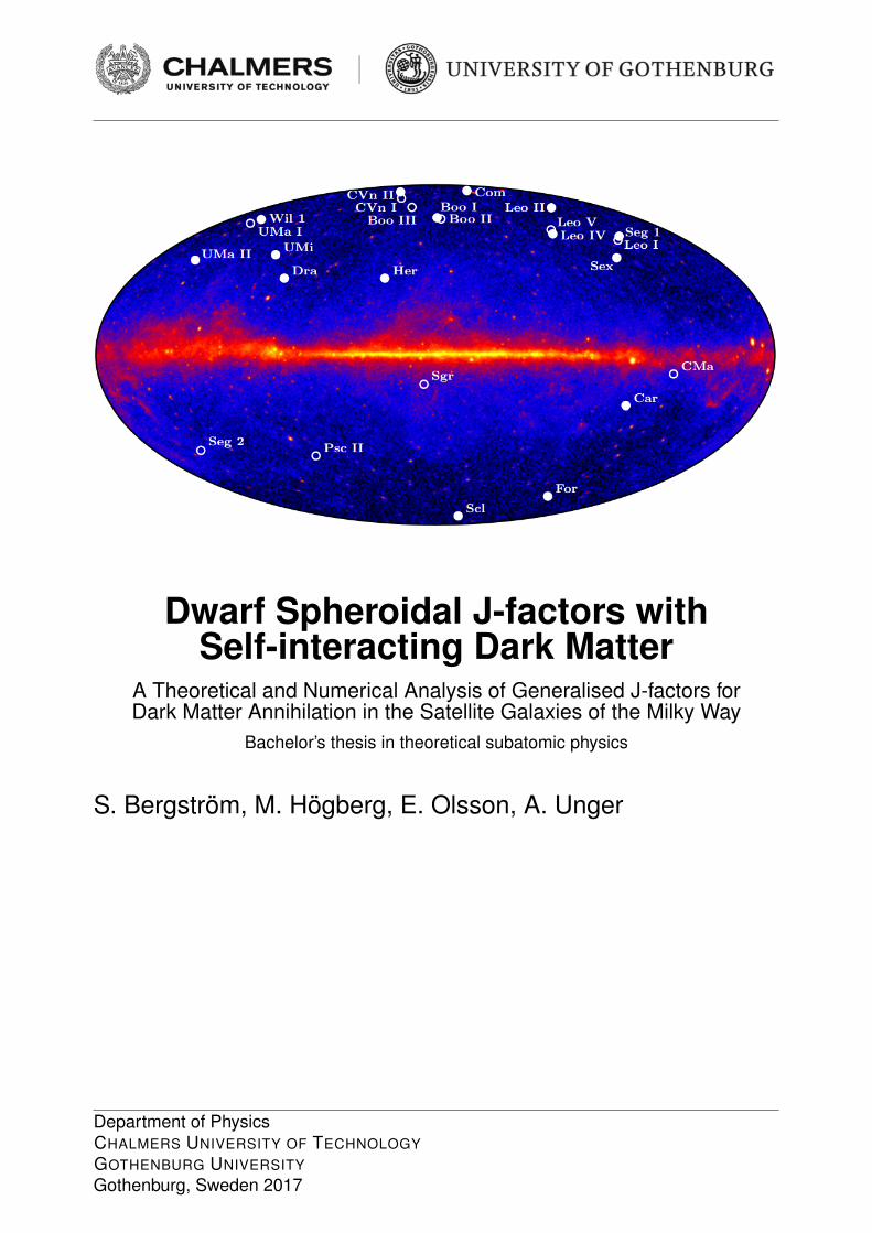
Cover: Known dwarf spheroidal satellite galaxies of the Milky Way overlaid on aHammer-Aitoff projection of a 4-year LAT counts map (E > 1 GeV). Credit goes toAckermann et al. [1].
Typeset in LATEXPrinted by [Name of printing company]Gothenburg, Sweden 2017
iv
Dwarf Spheroidal J-factors with Self-interacting Dark MatterA Theoretical and Numerical Analysis of Generalised J-factors forDark Matter Annihilation in the Satellite Galaxies of the Milky WaySEBASTIAN BERGSTRÖM, MICHAEL HÖGBERG, EMELIE OLSSON, ANDREASUNGERDepartment of PhysicsChalmers University of TechnologyGothenburg University
AbstractThe next decade of searches in the field of dark matter will focus on the detection ofgamma rays from dark matter annihilation in dwarf spheroidal galaxies. This darkmatter-induced gamma ray flux crucially depends on a quantity known as the J-factor. In current research, the J-factor calculations does not include self-interactionbetween the dark matter particles, but there are indications on galactic scales thatdark matter is self-interacting. The purpose of this thesis is to introduce a thoroughgeneralisation of the J-factor to include a self-interacting effect and to computethe factor for 20 dwarf spheroidal galaxies orbiting the Milky Way. We thoroughlystudy the fundamental theory needed to compute the J-factor, based on Newtoniandynamics and non-relativistic quantum mechanics. A maximum likelihood formal-ism is applied to velocity data from dwarf spheroidal galaxies, assuming a Gaussiandistribution for the line of sight velocity data. From this we extract galactic lengthand density scale parameters. The acquired parameters are then used to computethe J-factor. Using a binning approach, we present an error estimate in J . The usedmethod is compared to previously published results, by neglecting self-interaction.We perform the first fully rigorous calculation for the J-factor, properly taking intoaccount the dark matter velocity distribution. We can deduce that a previouslyused approximation of the self-interaction overestimates the J-factor by 1.5 ordersof magnitude. Furthermore, we confirm that our method produces three to fourorders of magnitudes larger values compared to J-factors without self-interaction.
Keywords: dark matter, J-factor, self-interacting, WIMP, annihilation.
v

SammanfattningDet kommande decenniets forskning om mörk materia kommer att fokusera på de-tektionen av gammastrålning från annihilation av mörk materia i sfäriska dvärg-galaxer. Flödet av gammastrålning som uppkommer vid mörk materia-annihilationhar ett centralt beroende av en kvantitet som kallas J-faktorn. I nuvarande forskn-ing inkluderas inte självinteraktion mellan mörk materia-partiklarna vid beräkningarav J-faktorn. Det finns dock indikationer på galaktisk skala att mörk materia ärsjälvinteragerande. Syftet med den här rapporten är att introducera den första rig-orösa generaliseringen av J-faktorn, där effekten av självinteraktion behandlas, ochberäkna faktorn för 20 sfäriska dvärggalaxer kring Vintergatan. Vi studerar nog-grant den grundläggande teorin som krävs för att beräkna J-faktorer, baserat påNewtonsk dynamik och icke-relativistisk kvantmekanik. En maximum likelihood-skattning används på data från dvärggalaxer, under antagandet att hastigheten förstjärnorna följer en Gaussisk distribution. Från detta extraheras parametrar förlängd- och densitetsskalan hos galaxen. De erhållna parametrarna används sedanför att beräkna J-faktorn. Genom att använda en sållningsmetod beräknas en felup-pskattning i J . Maximum likelihood-metoden tillämpas på fallet utan självinterak-tion för att jämföra med tidigare studier. Vi utför en utförlig beräkning av J-faktorndär hänsyn tas till den mörka materians hastighetsdistribution. Slutsatsen dras atten tidigare använd uppskattning överskattar J-faktorn med 1.5 storleksordningar.Dessutom kan vi bekräfta att vår metod ger tre till fyra storleksordningar störrevärde för J-faktorn jämfört med utan självinteraktion.
Nyckelord: mörk materia, J-faktor, självinteraktion, WIMP, annihilation.
vi

AcknowledgementsWe are very thankful to our supervisor Riccardo Catena, without whom this bach-elor project had not been possible. He has been a mediator of several fundamentalnon-SM forces; providing us with the theoretical material, the velocity data andthe overall knowledge to solve this task, not to mention his professional expertise inscientific writing. A special thanks to the other group working on the same project,Magdalena Eriksson, Björn Eurenius, Susanna Larsson and Rikard Wadman. Theyhave been a great support throughout the process with discussions on widely differ-ent physics concepts as well as fika buddies. It has been absolutely invaluable to beable to compare data with them when conducting new calculations.We also want to thank Andrea Chiappo for sending the data of the 20 dwarfspheroidal galaxies.
S. Bergström, M. Högberg, E. Olsson, A. Unger
Gothenburg, May 2017
viii

Contents
List of Figures xiii
List of Tables xv
1 Introduction 1
2 Background 22.1 Evidence for dark matter . . . . . . . . . . . . . . . . . . . . . . . . . 22.2 Why self-interacting WIMPs? . . . . . . . . . . . . . . . . . . . . . . 32.3 Current research and J-factors . . . . . . . . . . . . . . . . . . . . . . 52.4 Astrophysics . . . . . . . . . . . . . . . . . . . . . . . . . . . . . . . . 6
3 Theory 93.1 Constituents of the J-factor . . . . . . . . . . . . . . . . . . . . . . . 93.2 Relation to observable data . . . . . . . . . . . . . . . . . . . . . . . 103.3 Jeans equations . . . . . . . . . . . . . . . . . . . . . . . . . . . . . . 12
3.3.1 Collisionless Boltzmann Equation . . . . . . . . . . . . . . . . 123.3.2 The Jeans equations . . . . . . . . . . . . . . . . . . . . . . . 133.3.3 Spherical case . . . . . . . . . . . . . . . . . . . . . . . . . . . 15
3.4 Dark matter relative velocity distribution . . . . . . . . . . . . . . . . 163.4.1 Relative velocity distribution . . . . . . . . . . . . . . . . . . 163.4.2 Application of Jeans theorem . . . . . . . . . . . . . . . . . . 183.4.3 Eddington inversion formula . . . . . . . . . . . . . . . . . . . 19
3.5 Sommerfeld enhancement . . . . . . . . . . . . . . . . . . . . . . . . . 213.5.1 Yukawa potential . . . . . . . . . . . . . . . . . . . . . . . . . 223.5.2 Sommerfeld enhancement for an annihilation process . . . . . 223.5.3 The relation between the Sommerfeld enhancement and the
radial wave function’s asymptotic behaviour . . . . . . . . . . 25
4 Methods 274.1 Numerical calculation of the Sommerfeld enhancement . . . . . . . . 274.2 Numerical calculation of the dark matter velocity distribution . . . . 284.3 Likelihood estimation of the dark matter mass distribution . . . . . . 29
4.3.1 Reduction of parameters and singularity handling . . . . . . . 304.4 Perfoming the integrals to calculate the Js-factor . . . . . . . . . . . 304.5 Calculation of confidence intervals for the Js-factor . . . . . . . . . . 314.6 Validation of method and complementary calculations . . . . . . . . . 32
x
Contents
5 Results 335.1 Validation of statistical method . . . . . . . . . . . . . . . . . . . . . 335.2 Validation of the Sommerfeld enhancement and the velocity distribution 365.3 Js-factors for dSphs including self-interaction . . . . . . . . . . . . . . 38
6 Discussion 406.1 Comparison with previous results . . . . . . . . . . . . . . . . . . . . 406.2 The impact of a proper velocity distribution . . . . . . . . . . . . . . 41
7 Conclusion 42
References 43
A Mathematica code IA.1 Interpolated velocity dispersion function . . . . . . . . . . . . . . . . IIA.2 Maximum likelihood estimation for galactic parameters . . . . . . . . VA.3 Calculate J-factors . . . . . . . . . . . . . . . . . . . . . . . . . . . . VIIA.4 Dark matter velocity distribution in dSphs . . . . . . . . . . . . . . . IXA.5 Sommerfeld enhancement . . . . . . . . . . . . . . . . . . . . . . . . XIVA.6 Calculated Js interpolated function . . . . . . . . . . . . . . . . . . . XVII
xi

Contents
xii
List of Figures
2.1 The stars in each of the grey segments, at radius r1 and r2, acts withthe same net force on a star located where the lines intersect if thedensity of stars is uniform. This can be understood by comparing thegravitational force which decreases as r−2 with the amount of stars inthe segments which in three dimensions is proportional to r2. Thesetwo contributions cancel out which results in the same net force. . . . 7
3.1 A model where the circle represents the galaxy, l.o.s. is the line ofsight, r is the galaxy’s radius, α is the angle between the radius andthe l.o.s. and R is the orthogonal distance from the centre of thegalaxy to the l.o.s. vr and vθ are the radial and angular velocities. . . 11
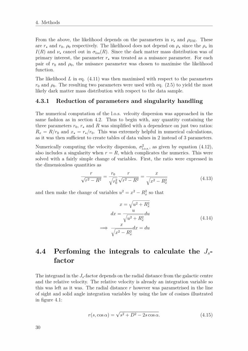
4.1 The galaxy seen from a distance D to it’s centre, with the radialdistance r from the galactic centre and the l.o.s. distance to theconcerned star s in the galaxy. α is the angle between D and s andθmax is the upper limit for the angular integration. . . . . . . . . . . . 31
5.1 The left figure shows all likelihood values less than 5 relative to theminimum value. The variable r0 range from 0.05 to 20 kpc and ρ0from 105 to 109 Mkpc−3. In the right figure a data binning methodhas been applied to select the points with the lowest likelihood. Theminimum likelihood is found J of 18.77. . . . . . . . . . . . . . . . . 33
5.2 Dashed contours specifying J values in the r0 and ρ0 plane. The greyboundaries defines confidence intervals from darker to lighter: 1-σ, 2-σ and 3-σ. The confidence intervals are constructed from calculationon Draco but the principle of a long flat valley is characteristic. . . . 35
5.3 The left plot shows the likelihood error estimation 1,2,3-σ from darkerto lighter shades of grey with the minimum showed by a red dot. Jsvalues are showed with dashed lines. The right hand plot shows thelikelihood versus the J value and gives the error estimations in levelsof 1,2,3-σ. Both plots are for data from Canes Venatici I, giving anexample for a galaxy with an inconsistent error estimation. . . . . . . 35
5.4 Sommerfeld enhancement factor for four different velocities as a func-tion of particle mass. Here α = 1
100 and mφ = 1 GeV/c2. The res-onance peak around 650 GeV/c2 is very dominant for low velocities,but vanishes for velocities over 10−3 c. . . . . . . . . . . . . . . . . . 36
xiii
List of Figures
5.5 Sommerfeld enhancement factor for five different masses as a functionof relative velocity. Here α = 1
100 and mφ = 1 GeV/c2. For all masses,the enhancements approach a constant value for low velocites. . . . . 37
5.6 Velocity distribution calculated from Eddington inversion formula,using typical values of r0 = 0.6 and ρ0 = 3.6 · 105, with emphasis onthat the feature but not scale is preserved when considering differentparameters. For smaller radii the distribution becomes more narrowand higher, giving more weight to lower velocities. The integral foreach curve is specified in the graph and is equal to unity. . . . . . . . 37
5.7 The left plot shows the likelihood error estimation 1, 2, 3 − σ fromdarker to lighter shades of grey with the minimum showed by a reddot. Js values are showed with dashed lines. The right hand plotshows the likelihood versus the Js value and indicates the error esti-mations in levels of 1, 2, 3− σ. Both plots are for data from Draco. . 39
5.8 A comparison of J values when using a constant velocity or the veloc-ity distribution for the Sommerfeld enhancement for Draco. ConstantSommerfeld enhancement, using (v∗ = 10−5c), is shown with the or-ange line, and accounting for the velocity distribution, is shown withthe blue line. . . . . . . . . . . . . . . . . . . . . . . . . . . . . . . . 39
xiv

List of Tables
5.1 Table comparing J-factors with Chiappo et al. [9]. Galaxies abovethe dashed line have a J which include the J from [9] within 1-σ.Missing 1-σ-levels are indicated with “-”. The difference is given as∆J , the log10 of the ratio between our and the referred J-factors.The last three columns are the optimised values for r?, r0 and ρ0. . . 34
5.2 Calculated J , Js and J S(v∗)s , and in the last column ∆J for Js and
J S(v∗)s . The galaxies have the same order as in table 5.1 and “-” are
indicating missing 1-σ-levels. . . . . . . . . . . . . . . . . . . . . . . . 38
xv

List of Tables
xvi
1Introduction
For a long time dark matter has been an elusive concept. The idea of some un-perceivable cosmic object has fascinated humans ever since the time of the ancientGreeks. Up until the end of the twentieth century it was believed we could notobserve the dark matter, thought to be made of faint stars, because of our lack oftechnology. Today, we know that dark matter does not emit radiation at all [2].
Dark matter is extensively studied since it explains a wide variety of astronomicalphenomena from galactic to cosmological scales [2]. One example is the discrepanciesin galactic rotation curves of disc galaxies. Assuming a dark matter halo explainsthis discrepancy [3]. It should be noted that this problem also can be solved withan adjustment of the theory of gravity, known as Modified Newtonian Dynamics [4].However, for many other phenomena, dark matter is the only plausible explanation.Examples of such are the collision of galaxies in the Bullet cluster and the large-scalestructure of the universe [5, 6].
Dark matter is assumed to consist of a new hypothetical particle outside the stan-dard model. Apart from its’ gravitational interaction, this particle interacts at mostweakly with ordinary matter. One of the most promising candidates for dark mattertoday is the Weakly Interacting Massive Particle (WIMP) (see [7] or [8]). Further-more, non-relativistic WIMPs have the strongest scientific support [2].
The annihilation, or decay, of WIMPs is assumed to generate gamma ray photons,among other standard model particles. This is the principle for indirect detection ofdark matter. The photon flux from WIMP annihilation in dwarf spheroidal galaxies(dSph) and the galactic centre can be measured, and a key part of this flux is calledthe J-factor. This J-factor has been computed for the Milky ways’ dwarf satellitegalaxies in previous research [9].
Even though cold WIMPs are the most promising candidate for dark matter, it cannot explain all phenomena. One of the most significant is the “Cuspy problem” [10].This can be solved by introducing the property of self-interaction for WIMPs. Suchan interaction alters the annihilation rate of WIMPs and in turn the J-factor.
The aim of this thesis is to generalise the J-factor to include self-interacting WIMPs.The self-interaction will be introduced as a Yukawa potential [11]. The theoreticalformalism will be based on Newtonian dynamics and non-relativistic quantum me-chanics. A likelihood estimation of the generalised J-factor will be done for 20 dSphsof the Milky Way. An error estimate to the J-factor will also be included.
1
2Background
In this chapter we present the theoretical background for both dark matter andthe presumed dark matter particles. Also, this chapter includes a brief review ofthe current research on dark matter, especially J-factors. The last section is anintroduction to some astrophysical concepts needed for the derivations in chapter 3.
2.1 Evidence for dark matter
Today, it is believed that 26% of the universe consist of dark matter, compared to5% ordinary matter [6]. It should also be mentioned that the rest is another conceptcalled dark energy, which has been introduced to explain the accelerating expansionof the universe. Dark energy does not have matter properties and should not beconfused with dark matter, even though they share a similar name.
The evidence for dark matter is today compelling. To begin with, the dynamicsof galaxy clusters would simply fall apart without the additional gravity from darkmatter. It is also needed to explain the velocity dispersion in galaxy clusters. Inthe first half of the twentieth century the astronomer Fritz Zwicky, one of the greatpioneers in the field of dark matter, calculated that the velocity dispersion of thegalaxies in the Coma Cluster without some form of invisible matter would be 10times smaller than the observed dispersion [2]. Another piece of evidence for darkmatter is the shape of the galactic rotation curves, where the velocities for thestars remain constant as distance from the galaxy’s centre increases. In theorieswithout dark matter, the velocities should behave precisely as in our own solarneighbourhood where the orbital velocity of the planets decrease with distance fromthe sun [3]. This indicates a smoother mass distribution than the one for the visiblemass which is clearly larger at the galactic centre. A halo of dark matter wouldexplain the constant velocities.
An additional example is the collision between two galaxies in the Bullet Cluster[5]. Astronomers who worked on the Hubble Space Telescope observed the colli-sion where the galaxies’ centres merged. When comparing data based on opticalobservations with data based on gravitational lensing they found an inconsistency.Dark matter could explain this inconsistency, since it only influences ordinary mat-ter gravitationally but very rarely collides with it. The ordinary matter will bounce
2
2. Background
in the collision, whereas the dark matter slips through smoothly. Also, dark matterexplains the extent of gravitational lensing observed.
Dark matter is also needed to explain the formation of the universe. The CosmicMicrowave Background (CMB) is electromagnetic radiation remaining from the re-combination, when the first atoms formed and light could propagate through theuniverse. This radiation is almost isotropic, but shows faint patterns, which wereestablished when gravity pulling in and photon pressure pushing out caused oscil-lations. Dark matter changes this pattern dramatically, since it is only affectedgravitationally and not by the photon pressure [6]. Without dark matter theseoscillations would prevent the formation of any lumps, and the large structure for-mation we observe today in the universe would not have been possible. Instead, thedark matter gets a head start when it comes to forming dense regions, and suchsimulations matches the distribution of galaxies and clusters we observe today.
Even though the evidence for dark matter is well established, there are a number oftheories about what dark matter actually is. One of the best candidates as of todayis the weakly interacting massive particle (WIMP), although many other candidatesexists. This particle might also fit the hypothesis of self-interaction very well, andis the main focus of this study.
2.2 Why self-interacting WIMPs?
There are several reasons for considering the WIMP as a dark matter candidate.First of all, if dark matter has a particle nature it could explain the observed grav-itational effects. Also, the observed flux of photons from many galaxies is todayhigher than the expected flux from the luminous matter. Annihilating dark matterparticles would explain this.
The reason for considering massive dark matter particles is because their mass hasto match the desired gravitational potential, without being numerous enough toannihilate into other kinds of particles or energy. The particles need to be weaklyinteracting with normal matter because the effects of dark matter has yet only beenseen in terms of gravitational effects and not by any other kind of interaction. Ifdark matter particles interacts through any other SM force with ordinary matter,this interaction must be by the weak force.
Furthermore, it has been found that dark matter consisting of WIMPs moving withnon-relativistic velocities, often denoted as cold particles, most accurately agreewith simulations of the formation of the early universe [2]. In the early universethe temperature was a lot higher, and consequently the energy sufficient for theWIMPs to both annihilate into and form from lighter particles. When the universecooled, the thermal energy of the lighter particles were no longer high enough toform WIMPs through annihilation. The amount of WIMPs decreased exponentially,since they could still annihilate into lighter particles, until the number density werelow enough for the annihilation to cease at large. The number of WIMPs todayis therefore approximately constant [7]. The low velocities will make the WIMPs
3
2. Background
clump together in clouds, since they can not overcome their mutual gravitationalforce.
A particle with larger cross section (i.e. the probability for the annihilation to occur)will in this model end up with a smaller number density, because it will annihilatefor a longer time. For dark matter, a cross section about the size of the weak nuclearforce would match the amount of WIMPs left in the Universe. A weakly interactingparticle with that annihilation cross section and a mass around 100 GeV is suggestedby the supersymmetric extension of the standard model. This coincidence is oftenreferred to as the ”WIMP miracle”
The WIMP is assumed to be its own antiparticle and one WIMP can therefore an-nihilate with any other WIMP. The high-energy photons (and other SM particles)produced in such an annihilation can be detected on Earth. However, even if annihi-lating WIMPs and luminous matter is considered, the observed flux of photons fromgalaxies will be higher than the calculated amount [12]. Introducing self-interactingWIMPs might equalise this relation, since it would increase the annihilation rateand in turn the flux of photons from the galaxies.
There is a variety of different models deciding both the WIMPs mass and the massof the mediator particle for the self-interaction. The strength of the interaction de-pends on the mass of the mediator particle. The current limit of the self-interactioncross section is σ/m < 2.23 · 10−24 cm2/GeV [13]. The dark matter mass is in therange 1 GeV - 100 TeV. In this thesis we use a model which assumes that dark matterannihilations is the origin of the whole discrepancy between observed and theoret-ically calculated flux of particles, which actually can originate from other sources.The WIMP is thought to have a mass around 500-800 GeV and the mediator particleof the self-interaction a mass of 1 GeV [8]. The WIMP is then heavier than the SMparticles, and therefore one can get a various number of different particles from theannihilation.
Introducing self-interaction might also solve other cosmological problems. One ofthe most impactful unsolved problems is known as the “Cuspy problem”. Thisproblem addresses a discrepancy between observed dark matter densities and sim-ulations. Simulations proposes cusped density profiles that diverges for small radii,in contrast to the observed ones that flatten out; so called cored profiles [14, 15].When simulations of the mass of the dSphs are compared to observations, it is foundthat the dSphs around the Milky Way should be more massive than observed. Thisis known as the “Too big to fail problem” and is also solver with self-interactingWIMPs.
Another problem is that the number of satellite galaxies is a lot lower than theexpected amount given from simulations, which is called the “Satellite problem”.All these problems can be solved by introducing self-interacting dark matter [10].With a self-interaction the WIMPs will not be able to clump together as much, sincethen they would annihilate more efficiently. This will change the halo density andmake it smoother. As an effect, the mass for the simulated dSphs will decrease andalso the number of substructures.
4
2. Background
Hence, there is a clear support of dark matter consisting of self-interacting WIMPs.The reasons mentioned in this section are also the reasons for this study to performcalculations based on self-interacting dark matter.
2.3 Current research and J-factors
Current research in astroparticle physics primarily focuses on detecting dark matterparticles from the cosmos and understanding their nature. Experiments search forphotons, charged antimatter or neutrinos produced in dark matter annihilation ordecay. The search is performed in dark matter dominated astrophysical objects,such as dSphs or the galactic centre. Detection strategies can be divides into twocomplementary approaches, known as direct and indirect detection. Direct detectionexperiments search for nuclear recoil events induced by the scattering of Milky Waydark matter particles in low-temperature detectors.
Indirect detection is based on the annihilation between dark matter particles. Asmentioned before, such annihilation produces standard model particles which can beobserved, particularly photons. To draw conclusions of the particle nature of darkmatter, one can compare the measured production of gamma rays in some regionin space with the theoretical value based on the number of stars emitting light inthat region. This thesis will contribute to the calculations of the flux of photonsoriginated from this dark matter particle annihilation.
The indirect dark matter searches are mostly based on observations of dSphs orbitingthe Milky way. The reason for this is the high proportion of dark matter relativeto ordinary matter in these galaxies and their symmetric near spherical shape. It isfor these reasons that star velocity data from a number of dSphs is the basis for ourcalculations.
In order to perform indirect searches, one must know the flux of particles originatingfrom dark matter particle annihilation. The flux, Γ, of a certain particle is propor-tional to the annihilation rate of dark matter. Γ is often expressed as a differentialrate over energies:
dΓdE ∝
∫∆Ω
∫l.o.s.〈σv〉ρ2
DM ds dΩ, (2.1)
where 〈σv〉 is the mean velocity cross section, ρDM is the dark matter density and∆Ω is the solid angle subtended by the stellar region, in our case a small galaxyorbiting the Milky Way (a dSph), as seen from the Earth. For a full descriptionof the flux, the branching ratio (a particle physics factor) should be included inequation (2.1), but a proper description of that is outside the scope of this thesis(consider instead Ferrer et al. [16]).
If the velocity averaged cross section, 〈σv〉, is constant throughout the galaxy, itcan be taken out of the integral. This is the case when the product σv is velocityindependent, which it is for the s-wave annihilation of self-interacting dark matter
5
2. Background
particles [17]. We denote the constant velocity averaged cross section by 〈σ0v〉. Thenone retrieves the so called J-factor for the galaxy, defined as
J =∫
∆Ω
∫l.o.s.
ρ2DM ds dΩ. (2.2)
By introducing a J-factor, the annihilation rate in eq. (2.1) can be fully separatedin an astrophysics and a particle physics part, corresponding to the J-factor and〈σ0v〉 respectively. Thus, calculating the J-factor for different dSphs is relativelystraightforward. It can be done using a maximum likelihood estimation as proposedby Chiappo et al. 2016 [9], which also will outline the approach in this thesis withsome minor modifications.
Self-interaction between particles is introduced by adding a potential to the Schrö-dinger equation describing the particle annihilation. Most commonly, this is donewith a Yukawa potential, which will be discussed later. This will introduce a velocitydependence in the product σv and as a result 〈σv〉 becomes non-constant through-out the galaxy. The simplification leading up to equation (2.2) is then no longerpossible. However, this velocity dependence can be encapsulated in what is calleda Sommerfeld enhancement factor, S(v), where 〈σv〉 = 〈S(v)σ0v〉. This will be de-scribed in more detail in section 3.5. The factor σ0v is now actually independent ofvelocity, and thus also of position in the galaxy and can be factored out of both theaverage and the integral in the same fashion as the simplification leading to (2.2).The new J-factor accounting for self-interaction will now include both astrophysicsand particle physics. In this thesis we define this as:
J` =∫
∆Ω
∫l.o.s.
ρ2DM 〈S(v)〉 ds dΩ. (2.3)
Note that for non self-interacting dark matter the Sommerfeld factor is unity, sothe expression in (2.3) can be taken as a general expression valid in either case. Wedenote this new factor J`, where ` = s, p, d, ... is the spectroscopic notation for thevalue of the orbital angular momentum quantum number ` used when solving theSchrödinger equation describing the annihilation.
2.4 Astrophysics
In order to present the necessary theoretical framework for this report, a reviewof some basic astrophysics must be done. In this section we present importantdefinitions and concepts and discuss some of the approximations that are made.
We define a galaxy to be an isolated stellar system. That is, the galaxy is bound by itsown gravitational force, the stars in the galaxy experience no notable gravitationalpull from other galaxies and collisions between galaxies are extremely rare.
The dynamics inside galaxies, as large systems consisting of many individual parti-cles (stars), can generally be described using statistical mechanics even though the
6

2. Background
galaxy is far from a gas. This approach is very useful, and often necessary, as itwould be impossible to fully describe systems of millions of stars using only New-ton’s equations. However, this must not be interpreted as stars generally behavingin the same way as, for example, gas molecules. In a gas, the particles do not overlong range at all, but instead interact strongly as they come close to each other.This is known as collisions and causes rapid acceleration of particles. In contrast,consider a star in a galaxy. The gravitational force from surrounding stars indeeddecreases with the distance as r−2 as per Newton’s law of gravitation. But, theamount of stars extorting gravitational pull on the very same star increases withdistance as r2, cancelling the decrease in gravitational strength. This is illustratedin figure 2.1. As such, in galaxies the long range interaction are also of importance.This implies that the motion of stars are dictated by the structure of the galaxy asa whole, rather than locally. One say that the dynamics in a galaxy is determinedby the large-scale gradient in the star density.
r1
r2
dr
dr
dΩ
Figure 2.1: The stars in each of the grey segments, at radius r1 and r2, acts withthe same net force on a star located where the lines intersect if the density of starsis uniform. This can be understood by comparing the gravitational force whichdecreases as r−2 with the amount of stars in the segments which in three dimensionsis proportional to r2. These two contributions cancel out which results in the samenet force.
However, it is not always enough to consider the large-scale gradient in the stardensity. Consider a star travelling through a galaxy. If the star encounters anotherstar very close on, its course will be somewhat perturbed from the description givenby the large-scale gradient in the star density. That is because the motion resultingfrom the encounter is highly dependent on the exact positions of the two stars. Ifthe perturbation is small compared to the unperturbed velocity, one can define therelaxation time, τrelax, as the time it takes for the total perturbation in the star’svelocity from multiple encounters to be of the same order as the velocity would havebeen without the perturbation [18]. This perturbation of a star’s velocity duringone crossing of the galaxy depends on how many stars it encounters.
7
2. Background
For a galaxy younger than the time it takes for a star to cross the galaxy, or a largergalaxy with less stars, the stars has not been significantly perturbed. The systemcan then be considered a collisionless system, in which a star move under a meanpotential generated by all the other stars. The dSphs around the Milky Way areyoung enough to be collisionless. In an old or high number density galaxy, as theMilky Way itself, the stars have been perturbed so many times that they do notfollow the large-scale gradient, and are not to be considered collisionless.
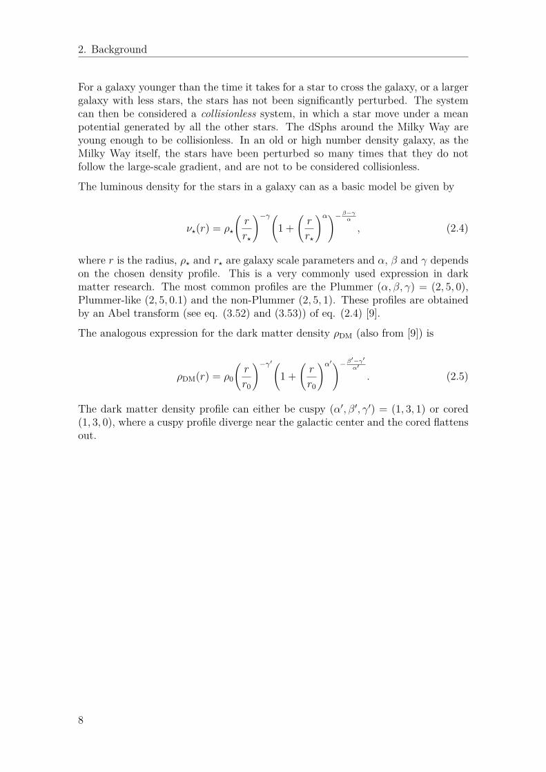
The luminous density for the stars in a galaxy can as a basic model be given by
ν?(r) = ρ?
(r
r?
)−γ(1 +
(r
r?
)α)−β−γα
, (2.4)
where r is the radius, ρ? and r? are galaxy scale parameters and α, β and γ dependson the chosen density profile. This is a very commonly used expression in darkmatter research. The most common profiles are the Plummer (α, β, γ) = (2, 5, 0),Plummer-like (2, 5, 0.1) and the non-Plummer (2, 5, 1). These profiles are obtainedby an Abel transform (see eq. (3.52) and (3.53)) of eq. (2.4) [9].
The analogous expression for the dark matter density ρDM (also from [9]) is
ρDM(r) = ρ0
(r
r0
)−γ′(1 +
(r
r0
)α′)−β′−γ′α′
. (2.5)
The dark matter density profile can either be cuspy (α′, β′, γ′) = (1, 3, 1) or cored(1, 3, 0), where a cuspy profile diverge near the galactic center and the cored flattensout.
8

3Theory
The first part of this chapter contains the definition of the J`-factor, together with apresentation of the necessary quantities for the calculation of J`. The next part willdescribe the underlying theory required to connect the J` to an observable. Morespecifically, the relation between the dark matter density and the velocity dispersionof the stars in a galaxy is derived. Finally, derivations and calculations of F (v) andS(v) will be presented to fully understand the framework.
3.1 Constituents of the J-factor
As presented in the end of the introduction, the J-factor for a dSph with self-interacting dark matter will look like eq. (2.1). In this study, the Schrödingerequation with a Yukawa potential will be solved for angular momentum quantumnumber l = 0, and thus we consider Js:
Js =∫
∆Ω
∫l.o.s.
ρ2DM〈S(v)〉 ds dΩ. (3.1)
Here, ρDM is the dark matter mass distribution and S(v) is the Sommerfeld en-hancement factor. The factor 〈S(v)〉 can be expressed as
∫F (v)S(v)d3v, with F (v)
as the dark matter velocity distribution;
Js =∫
∆Ω
∫l.o.s.
ρ2DM
∫F (v)S(v) d3v ds dΩ (3.2)
To be able to calculate Js, models of the components ρDM, F (v) and S(v) arerequired.
The Sommerfeld enhancement factor, S(v), is based on particle physics and will beapproached theoretically. More specifically, a derivation of S(v) under the assump-tion of a Yukawa potential in the Schrödinger equation describing the annihilationwill be done in section 3.5.
The determination of F (v) is an astrophysical problem. For a galaxy which isspherically symmetric with respect to its gravitational potential and isotropic withrespect to its velocity distribution, F (v) can be uniquely determined from ρDM [18].
9
3. Theory
In this study we will perform the calculations on the dSphs based on these twoassumptions. The problem of determining F (v) is therefore reduced to deriving therelation between ρDM and F (v). This is shown in section 3.4.
The remaining problem is to determine ρDM , the dark matter mass distribution. Itcan not be observed directly. Instead, a theoretical connection must be establishedbetween ρDM and some directly observable quantity. In this thesis we have chosenthe velocity dispersion of the stars in the dSph. This theoretical connection will bederived in the following two sections, 3.2 and 3.3. The result is seen in the methodsection 4.3 in eq. (4.12).
3.2 Relation to observable data
In a spectrum from a galaxy far away one actually sees the superposition of manystellar spectra, with a Doppler shift depending on the stars’ motion. This is becausethe galaxy is seen as just a disc and not a 3-dimensional object. By integrating thespectrum of the whole galaxy one gets a spectrum with broader absorption lines asa result of the motions of the stars. From this the velocity dispersion of the stars,σl.o.s. is determined.
The velocity dispersion along the line of sight, σ2l.o.s., is given by
σ2l.o.s. = 1
N
N∑j=1
(vl.o.s.j − vl.o.s.)2, (3.3)
where vl.o.s.j is the l.o.s velocity for star j and N is the number of stars in a cylinder of
volume dA · dl. The latter can be calculated by integrating over the spatial density,ν(r);
dN = dA∫
∆ldl ν(r). (3.4)
The integration variables dA and dl can be visualised as an infinitesimal cylinderalong the line of sight in fig. 3.1. The following change of variable can be explainedby the figure: dr = dl cosα, where cosα =
√r2−R2
r. The limits comes from an
integration from 0 to ∞ with the approximation of the galaxy being infinitely faraway from the observer. This is then equivalent to an integration from R to ∞multiplied by 2 and results in the following expression;
dN = dA 2∫ ∞R
drr√
r2 −R2ν(r). (3.5)
10

3. Theory
vr
vθ
l.o.s.r
Rα
Figure 3.1: A model where the circle represents the galaxy, l.o.s. is the line ofsight, r is the galaxy’s radius, α is the angle between the radius and the l.o.s. andR is the orthogonal distance from the centre of the galaxy to the l.o.s. vr and vθ arethe radial and angular velocities.
It is not possible to measure ν(r), but the luminosity density ν∗(r) is an observable.Therefore, the surface brightness I(R) id defined as N
dA [18]. I(R) is then
I(R) = 2∫ ∞R
drr√
r2 −R2ν∗(r). (3.6)
vl.o.s. in eq.(3.3) is defined by
vl.o.s. = 1N
N∑j=1
vl.o.s.j . (3.7)
In this expression vl.o.s.j for a single star can not be predicted, but one can predict an
average over the entire sample of stars, 〈vl.o.s.j 〉. This quantity can, with help fromfig. 3.1, be written as 〈vl.o.s.j 〉 = 〈vr〉 cosα−〈vθ〉 sinα, where vr and vθ are the radialand angular velocities respectively. Making the approximation of a static galaxygives that 〈vr〉 and 〈vθ〉 are both zero. This makes vl.o.s. approximately zero. In eq.(3.3) only the term (vl.o.s.
j )2 remains in the sum for σ2l.o.s.. With 〈vrvθ〉 = 0 due to
the spherical symmetry this gives
(vl.o.s.j )2 ≈ 〈(vl.o.s.j )2〉 = 〈v2
r〉 cos2 α− 〈v2θ〉 sin2 α. (3.8)
Again from fig. 3.1, cos2 α = r2−R2
r2 and sin2 α = R2
r2 . Putting this in the aboveequation and simplifying by introducing β = 1− 〈v2
θ〉/〈v2r〉 gives
〈(vl.o.s.j )2〉 = 〈v2
r〉(
1− R2
r2 β(r)). (3.9)
11
3. Theory
β is a velocity anisotropy parameter for the galaxy that describes the relation be-tween the radial and tangential velocity dispersions, see eq. (3.33). Summation of〈(vl.o.s.
j )2〉 over the stars j in the differential volume dAdl yields
∑j
〈(vl.o.s.j )2〉 = dA dl ν∗(r) 〈v2r〉(
1− R2
r2 β(r)). (3.10)
Dividing by I(R), integrating along the l.o.s. and with the same change of variableas in eq.(3.5), results in
σ2l.o.s. = 2
I(R)
∫ ∞R
dr ν?(r) 〈v2r〉(
1− R2
r2 β(r))
r√r2 −R2
. (3.11)
The quantity ν∗(r) 〈v2r〉 is obtained in section 3.3 through Jeans equations.
3.3 Jeans equations
This section is dedicated to derive the theoretical connection between the averageradial velocity of stars squared, 〈v2
r〉, and the density of a galaxy. This leads toa relation between our line-of-sight velocity dispersion data and the dark matterdensity, if one assumes that most of the galaxy’s mass consist of DM.
3.3.1 Collisionless Boltzmann Equation
Given the assumptions made above, one can describe a galaxy by the collisionlessBoltzmann equation. This can be shown by a simple line of reasoning, as follows.
Consider a galaxy young enough to be considered collisionless with a distributionfunction (DF) f(x,v, t). Now, we can describe the coordinates by a 6-dimensionalvector in phase-space, so that
(x,v) = w ≡ (w1, ..., w6). (3.12)
As stars move inside the galaxy, the points in phase-space changes. If the stars inthe galaxy experience a smooth gravitational potential, Φ(x, t) the velocity of theflow of coordinates is
w = (x, v) = (v,−∇xΦ). (3.13)
Given knowledge of w for every star in the galaxy at some initial time, say t0, wouldby Newtons laws allow us to extract w at any later time t. Since the stars movesmoothly through the galaxy, the flow w satisfies the continuity equation, with thedensity f(w, t), given by∫
V
∂f(w, t)∂t
d3x = −∫∂Vf(w, t)w · d2S. (3.14)
12

3. Theory
In the rest of this section we will omit the arguments of f . Now, using the divergencetheorem on the right hand side and moving it to the left hand side yields
∫V
[∂f
∂t+∇w · fw
]d3x = 0. (3.15)
Note that the divergence operator is now acting in all 6 phase-space coordinates.Since this must hold for all volumes, we can remove the integral. Expanding thedivergence operator gives
∂f
∂t+ f∇w · w︸ ︷︷ ︸
=0
+w · ∇wf = 0 (3.16)
The property that∇w ·w = 0 follows from vi and xi being independent phase-spacevariables and that the force, −∇xΦ, is velocity independent so that
∂vi∂xi
= 0
∂vi∂vi
= ∂
∂vi(−∇xΦ) = 0
(3.17)
and we arrive at the collisionless Boltzmann equation
∂f
∂t+ w · ∇wf = 0. (3.18)
In Cartesian coordinates, this is
∂f
∂t+ v · ∇xf −∇xΦ · ∂f
∂v= 0. (3.19)
3.3.2 The Jeans equations
Solving the collisionless Boltzmann equation is extremely hard, as f is a functionof seven variables. One can however extract valuable information regarding thesolution, by taking moments of the equation. This will lead to Jeans equations,which provide an important connection between the mean radial velocity squaredand the mass of the galaxy.
First, we define the spatial density, ν, and the mean velocity, 〈v〉 = (〈v1〉, 〈v2〉, 〈v3〉),of the stars as
ν ≡∫f d3v
〈vi〉 ≡1ν
∫fvi d3v.
(3.20)
13
3. Theory
We can now study the zeroth moment of equation (3.19) by integrating over allvelocities. Adopting the summation convention and writing the equation componentwise then yields
∫ ∂f
∂td3v +
∫vi∂f
∂xid3v−
∫ ∂Φ∂xi
∂f
∂vid3v = 0. (3.21)
From the first two terms, we can take the time derivative and the spatial derivativesoutside the integrals, as they do not depend on velocity. The third term vanishes,by application of the divergence theorem and knowing that no stars move infinitelyfast, that is f → 0 as |v| → ∞. We thus arrive at
∂
∂t
∫f d3v︸ ︷︷ ︸=ν
+ ∂
∂xi
∫vif d3v︸ ︷︷ ︸=ν〈vi〉
− ∂Φ∂xi
∫|v|=∞
f d2v︸ ︷︷ ︸=0
= 0
⇐⇒ ∂ν
∂t+ ∂(ν〈vi〉)
∂xi= 0
(3.22)
This is a continuity equation in ν and more commonly known as the first Jeanequation.
We proceed our analysis by taking the first moment of equation (3.19), which isdone by multiplying with vj and integrating over all velocities.
∫vj∂f
∂td3v +
∫vjvi
∂f
∂xid3v−
∫vj∂Φ∂xi
∂f
∂vid3v = 0. (3.23)
Again, we can take time and spatial derivatives outside the integrals, as well as thegravitational potential Φ. The equation simplifies to
∂
∂tν〈vj〉+ ∂
∂xiν〈vjvi〉 −
∂Φ∂xi
∫vj∂f
∂vi= 0 (3.24)
where we have defined〈vjvi〉 = 1
ν
∫vjvif d3v. (3.25)
The third term of equation (3.24) can be simplified, integrating once by parts, inthe following fashion
∂Φ∂xi
∫vj∂f
∂vi= ∂Φ∂xi
∫ ∂vj∂vi
f d3v = ∂Φ∂xi
δjiν = ν∂Φ∂xj
(3.26)
and we arrive at∂
∂tν〈vj〉+ ∂
∂xiν〈vjvi〉 − ν
∂Φ∂xj
= 0 (3.27)
which is the second Jean equation. Now, define the velocity dispersion tensorσ2ij = 〈vivj〉 − 〈vi〉〈vj〉, expand the first and second term in equation (3.27) by the
product rule and subtract by equation (3.22) multiplied by 〈vj〉. This yields
14
3. Theory
ν∂〈vj〉∂t
+
〈vj〉∂ν
∂t+ ∂
∂xi
(νσ2
ij
)+
〈vj〉∂ν〈vi〉∂xi
+ ν〈vi〉∂〈vj〉∂xi
− ν ∂Φ∂xj
−
〈vj〉∂ν
∂t−
〈vj〉∂ν〈vi〉∂xi
= 0.(3.28)
Rearranging the terms gives the final result
ν∂〈vj〉∂t
+ ν〈vi〉∂〈vj〉∂xi
= −ν ∂Φ∂xj− ∂
∂xi
(νσ2
ij
)(3.29)
known as the third Jean equation.
3.3.3 Spherical case
While there exists a general set of Jeans equations in spherical coordinates, we willnot go through those derivations. Instead, we will make assumptions relevant forthe dSphs we will look at, in order to extract the expression for 〈v2
r〉.
First of all, we consider only stationary galaxies. This implies that all derivativeswith respect to time is zero and that 〈vr〉 = 0; if the radial velocities do not cancel inmean value, our galaxy would be expanding or shrinking. Furthermore, we assumespherical symmetry. This leads to a gravitational potential only dependent on theradius, r, and that 〈vθ〉 = 〈vφ〉 = 0.
With the assumptions above, the left hand side of equation (3.29) vanishes. Fur-thermore, we get
− ν ∂Φ∂xj
= −ν ∂Φ∂r
r = −νGM(r)r2 r (3.30)
where G is Newton’s gravitational constant and M(r) =∫ r
0 ρ(s) ds is the enclosedgalaxy mass at radius r for a spatial density ρ(s). We note here that for dSphs, thedark matter density is much larger than the density of ordinary matter, and thereofρ(s) can be replaced by the dark matter density, ρDM . Thus, this expression yieldsthe desired connection to ρDM. Now, equation (3.29) simplifies to
∂
∂xi
(νσ2
ij
)= −νGM(r)
r2 r (3.31)
The left hand side of this equation is a tensor divergence term. In it most gen-eral form, this a tedious expression i spherical coordinates. But as can be seenin equation (3.30) we are only interested in the radial component of this expres-sion. Furthermore, due to the spherical symmetry all mixed terms in the velocitydispersion tensor are zero. This simplifies the spherical tensor divergence to
∂νσ2rr
∂r+ 2νσ
2rr
r− 1r
(νσ2θθ + νσ2
φφ) = −νGM(r)r2 . (3.32)
15
3. Theory
Since σ2ii = 〈v2
i 〉 we get a differential equation in ν〈v2r〉
∂ν〈v2r〉
∂r+ 2βν〈v
2r〉r
= −νGM(r)r2 ,
β ≡ 1−〈v2θ〉+ 〈v2
φ〉2〈v2
r〉
(3.33)
where β is a velocity anisotropy parameter for the galaxy. While the general solutionto equation (3.33) is straightforward, we are only concerned with galaxies assumedto be isotropic, i.e. 〈v2
θ〉 = 〈v2φ〉. Consequently, β = 0 and the solution to the
differential equation in this case is
ν〈v2r〉(r) = −
∫ ν(r)GM(r)r2 dr + C. (3.34)
To obtain the solution as a definite integral, we note that the quantity ν〈v2r〉 → 0
as r →∞ and thus we can set C = 0 and write the solution as
ν〈v2r〉(r) =
∫ ∞r
ν(s)GM(s)s2 ds . (3.35)
As mentioned in section 3.2 the spatial density ν is not an observable, but theluminosity density ν? is. With them being proportional, and the relation hidden inthe luminosity profile (eq. (2.4)), eq. (3.35) becomes
ν?〈v2r〉(r) =
∫ ∞r
ν?(s)GM(s)s2 ds . (3.36)
3.4 Dark matter relative velocity distribution
By regarding two particles at a time in the annihilation process it is possible to usethe reference frame for one of them. In this section we will expand this argumentand develop an expression for the relative velocity distribution, in terms of the massdistribution using Eddington’s inversion formula.
3.4.1 Relative velocity distribution
As we will argue in 3.5 only two particles will be taken into account during theannihilation. The probability for an annihilation of two particles will depend onboth their velocities, due to that the velocities are used in the Sommerfeld enhance-ment. Therefore the annihilation rate will be proportional to both particles velocitydistributions as described in
Js ∝∫
d3v1d3v2Fx(v1)Fx(v2)S(v). (3.37)
S(v) is the Sommerfeld enhancement which is discussed below, in section 3.5, andFx(v) is the velocity distribution of one particle at position x.
16
3. Theory
By using the relative velocity in the center of mass frame one can simplify theexpression. The probability of the particles having center of mass velocity vcm =(v1 + v2)/2 and relative velocity vrel = v1 − v2 must be equal to the probability ofthem having velocities v1 and v2. Noting that d3v1d3v2 = d3vcmd3vrel, the changeof variables give
Fx(v1)Fx(v2)d3v1d3v2 = Fx(vcm + vrel/2)Fx(vcm − vrel/2)d3vcmd3vrel. (3.38)
Js depends only on the relative velocity, since the centre of mass velocity does notdescribe how the particles move closer together and annihilation is local, see belowin section 3.5.2. Therefore the above expression can be integrated over vcm to obtainthe relative velocity distribution,
Fx,rel(vrel) d3vrel =∫Fx(vcm + vrel/2)Fx(vcm − vrel/2)d3vcm d3vrel. (3.39)
To make further simplifications the properties of the distribution Fx(v) need to bedeveloped.
At a point x in the halo the dark matter velocity distribution, Fx(v), can by defini-tion be written as
Fx(v)d3v ≡ f(x,v)ρ(x) d3v, (3.40)
where f(x,v) is the phase-space density and ρ(x) is the dark matter mass distribu-tion, which can be defined as ρ(x) ≡
∫f(x,v)d3v [16]. We make the assumptions
that the mass distribution is spherically symmetric, i.e. ρ(x) = ρ(r), and that thevelocity is isotropic. As a result the phase space density only depends on the radii,r, and the magnitude of the velocity, f(x,v) = f(r, v). Therefore the the veloc-ity distribution is independent of direction, i.e. Fx(v)d3v = Fr(v) dv and the twodirections can be integrated out:
Fr(v) dv = 4πv2f(r, v)ρ(r) dv . (3.41)
With this we can rewrite equation (3.39) as
Fr(vrel) dvrel = 4πv2rel
∫ f(r, |vcm + vrel/2|)f(r, |vcm − vrel/2|)ρ2(r) d3vcmdvrel. (3.42)
The argument |vcm ± vrel/2| is independent of one angle, thus 2π can be integratedout. The other angle is between vcm and vrel and therefore |vcm ± vrel/2| = vcmz ±vrel/2, z ∈ [−1, 1]. Then the relative velocity distribution is
Fr(vrel) dvrel = 8π2v2rel
∫ ∞0
v2cm
∫ 1
−1
f(r, vcmz + vrel/2)f(r, vcmz − vrel/2)ρ2(r) dz dvcm dvrel,
(3.43)where the subscript r in Fr(vrel) indicates that this velocity distribution is for onespecific radii. f is the phase space distribution and ρ is the mass distribution.
17
3. Theory
3.4.2 Application of Jeans theorem
As mentioned above (section 3.3.2) the collisionless Boltzmann equation almostimpossible to solve, since it is a function of seven variables. To obtain exact solutionsone can regard only a subset of all possible stellar dynamical equilibria at a time.This will be done for steady-state dSphs, in order to obtain Eddington’s formula inthe next section.
We base the derivation on the Jeans theorem (Binney and Tremaine, p. 200, [18]):
Any steady-state solution to the collisionless Boltzmann equation depends on thephase-space coordinates only through integrals of motion in the galactic potential,and any function of the integrals yields a steady-state solution of the collisionlessBoltzmann equation.
Assuming a steady-state spherically symmetric system, the distribution function(DF) is a function of the energy, E, and the angular momentum, L. E is an integralof motion in any static potential and L is in an spherical potential constituted bythree integrals of motion. An integral of motion is any function of (x,v) that isconstant along any orbit. By the Jeans theorem, any non-negative function of thementioned integrals can be the DF of a spherical stellar system. Due to the sphericalsymmetry the function will only depend on the magnitude of L. With f as the DF,and for a stellar system that itself provides the potential Φ, one has
∇2Φ = 4πGρ = 4πG∫f d3v . (3.44)
The same equation after exploiting spherical symmetry (Φ depends only on r) iscalled the fundamental equation of spherical equilibrium stellar systems, and isdefined by
1r2
ddr
(r2 dΦ
dr
)= 4πG
∫f(1
2 |v|2 + Φ|r× v|
)d3v . (3.45)
To simplify future calculations, the relative potential Ψ and the relative energy Eare defined as
Ψ = −Φ + Φ0 (3.46)and
E = −E + Φ0 = Ψ− 12v
2, (3.47)
with Φ0 chosen to satisfy f > 0 for E > 0 and f = 0 for E 6 0. The relativepotential then satisfies Poisson’s equation through ∇2Ψ = −4πGρ, where Ψ → Φ0as x→∞.
For a system with isotropic velocity-dispersion tensor the DF will depend only on Eand not L. Eq. (3.45) then becomes (in spherical coordinates)
1r2
ddr
(r2 dΦ
dr
)= −4πG
∫ √2Ψ
0f(E)4πv2dv = −16π2G
∫ √2Ψ
0f(Ψ− 1
2v2)v2 dv ,
(3.48)
18

3. Theory
where the upper limit is decided by f 6= 0 for E = Ψ − 12v
2 > 0. A change ofvariable from v to E in eq. (3.48), with dE = −vdv and limits v = 0→ E = Ψ andv =√
2Ψ→ E = 0, results in
1r2
ddr
(r2 dΦ
dr
)= −16π2G
∫ Ψ
0f(E)
√2(Ψ(r)− E) dE . (3.49)
3.4.3 Eddington inversion formula
With the Eddington inversion formula one can derive the DF f(E) for any givenmass density ρ(r). f(E) will then be used to compose a velocity distribution, whichwill take part in eq.(3.43). The theory from the former section is used.
To achieve this formula for the density, notice that Ψ is an monotonic function of r,due to the spherical symmetry, and use the same change of variable as in eq.(3.49):
ρ(r) =∫fd3v = 4π
∫v2f
(Ψ− 1
2v2)dv = 4π
∫ Ψ
0f(E)
√2(Ψ(r)− E)dE (3.50)
The above equation is then differentiated with respect to Ψ, resulting in
1√8π
dρdΨ =
∫ Ψ
0
f(E)√Ψ(r)− E
dE . (3.51)
This is an Abel integral on the form
f(x) =∫ x
0
g(t)dt(x− t)α , 0 < α < 1 (3.52)
which has the solution [18]
g(t) = sin(πα)π
∫ t
0
f(x)dx(t− x)1−α . (3.53)
The above formula for solving the Abel integral gives the following solution toeq.(3.51)
f(E) = 1√8π2
ddE
∫ E0
dΨ√E −Ψ(r)
dρdΨ . (3.54)
Since f(E) > 0 everywhere, the function∫ E0
dΨ√E−Ψ(r)
has to be an increasing functionof E . Otherwise, the solution is unphysical. Applying Leibniz integral rule oneq.(3.54) gives the alternative form, which is called Eddington’s formula;
f(E) = 1√8π2
∫ E0
dΨ√E −Ψ(r)
d2ρ
dΨ2 + 1√E
(dρ
dΨ
)Ψ=0
. (3.55)
19
3. Theory
This expression is rewritten with help from the chain rule, since ρ is not usuallygiven as a function of Ψ:
d2ρ
dΨ2 =(dΨ
dr
)−2 d2ρ
dr2 + d2r
dΨ2dρdr and d2r
dΨ2 = −d2Ψdr2
(dΨdr
)−3(3.56)
givesd2ρ
dΨ2 =(dΨ
dr
)−2(d2ρ
dr2 −(dΨ
dr
)−1 d2Ψdr2
dρdr
). (3.57)
From a numerical point of view it is easier to change the variable to the radiusof the spherical system, r, according to dΨ = dΨ
dr dr. Assuming only dark mattercontributes to the gravitational potential and the density, eq. (3.55) becomes
f(E) = 1√8π2
∫ ∞Ψ−1DM (E)
1√E −ΨDM(r)
×
dρDMdr
d2ΨDM
dr2
(dΨDM
dr
)−2− d2ρDM
dr2
(dΨDM
dr
)−1dr. (3.58)
From this DF f(E) one can reach a velocity distribution by making use of therelation in eq. (3.47), namely E = Ψ(r) − 1
2v2. f(E) then becomes f(Ψ(r) − 1
2v2).
This f(Ψ(r) − 12v
2) is identified as the f(r, v) from eq.(3.43) in section 3.4.1, withv = vcmz ± vrel/2, namely
Fr(vrel) dvrel = 8π2v2rel×∫ ∞
0v2
cm
∫ 1
−1
f(r, vcmz + vrel/2)f(r, vcmz − vrel/2)ρ2(r)DM
dz dvcm dvrel.(3.59)
Noticing that the integrand is symmetric in z, giving a factor 2 when integratingfrom 0 to 1 instead, and using that v2 = v2
cm/2 + v2rel/8 ± vcmvrelz/2, the relative
velocity distribution becomes
Fr(vrel) dvrel = 16π2v2rel
ρ2DM(r)
∫ ∞0
v2cm
∫ 1
0f(
Ψ(r)− v2cm2 −
v2rel8 −
vcmvrelz
2
)×
f(
Ψ(r)− v2cm2 −
v2rel8 + vcmvrelz
2
)dz dvcm dvrel.
(3.60)
Combining these two equations gives further limitations to the integration bound-aries in eq. (3.60), since f(E) = 0 for E 6 0 (as discussed after eq. (3.47)). E > 0gives Ψ(r)− 1
2v2 > 0 → v2 6 2Ψ(r) and the maximum v2 = v2
cm + v2rel/4 + vcmvrelz
gives2Ψ > v2
cm + v2rel4 ± vcmvrelz ⇐⇒ z 6
8Ψ− 4v2cm − vrel
4vcmvrel. (3.61)
Combining v2 6 2Ψ(r) with 0 6 z 6 1 results in the following inequalities, the firstfor z = 1
v2cm + v2
rel4 + vcmvrel =
(vcm + vrel
2)2
6 2Ψ ⇐⇒ vcm 6√
2Ψ− vrel
2 (3.62)
20
3. Theory
and the second for z = 0
v2cm + v2
rel4 6 2Ψ ⇐⇒ vcm 6
√8Ψ− v2
rel
2 . (3.63)
These integration limits give the final expression for relative velocity distribution:
Fr(vrel) dvrel = 16π2v2rel
ρ2(r)DM×
∫ √2Ψ− vrel2
0v2
cm
∫ 1
0A dz dvcm +
∫ √8Ψ−v2rel
2√
2Ψ− vrel2
v2cm
∫ 8Ψ−4v2cm−vrel
4vcmvrel
0A dz dvcm
where
A = f(
Ψ(r)− v2cm2 −
v2rel8 −
vcmvrelz
2
)f(
Ψ(r)− v2cm2 −
v2rel8 + vcmvrelz
2
).
(3.64)
3.5 Sommerfeld enhancement
One of the most important physical quantities in nuclear and particle physics is thecross section. Classically, this is the area transverse to the relative motion of twoparticles within which a scattering process, a particle collision, can occur. However,a scattering process is intrinsically stochastic: even if the particles meet withinthe cross section area, the particle collision might still not occur [19]. The morerigorous formulation of the cross section therefore relies on quantum mechanics.Given a probability density current, the cross section times this equals the numberof scattered particles. The cross section is thus proportional to the probability ofcollision between two particles. Since annihilation of two particles is nothing morethan a particle collision resulting in a transformation of the particles, the importanceof the cross section for an annihilation process is indisputable.
If there exists a long-range potential between the particles, the cross section willchange due to some form of force between the particles. If the force is attractive thecross section will be greater and if it is repulsive it will be smaller. When a poten-tial between the particles is accounted for it is called a Sommerfeld enhancement.It is also important to note that the Sommerfeld enhancement is usually referredto in non-relativistic quantum mechanics. The new cross section due to the poten-tial is always proportional to the old one not accounting for the same. Thus theSommerfeld enhancement can be expressed as a Sommerfeld enhancement factor:
σ = S(v)σ0 (3.65)
where σ0 is the old cross section, σ the new one and S the Sommerfeld enhancementfactor with a dependence on the relative velocity v. In the two next paragraphs, adescription of the Yukawa potential and a derivation of the enhancement factor Sfollows.
21
3. Theory
3.5.1 Yukawa potential
In particle physics, a force between two particles can be described as an exchangeof a force mediator particle. The properties of this exchange particle affects theproperties of the force [11]. The Yukawa potential describes one such force and hasthe form;
VY ukawa(r) = αe−mφr
r(3.66)
where α is the strength of the potential, r the radial coordinate and mφ the massof the mediator particle. The Coulomb potential is a special case of the Yukawapotential where the force exchange particle, the photon, has zero mass. The Yukawapotential corresponds to a long-range force which can describe the self-interactionbetween dark matter particles. Thus, it can lead to a Sommerfeld enhancement.Nonetheless, it is very simple in its form. It is for these reasons it has been chosenas the subject potential for this study.
3.5.2 Sommerfeld enhancement for an annihilation process
To fully derive the Sommerfeld enhancement, one must refer to quantum field theory.This is beyond the scope of this report. Instead, we will derive an expression of howan elastic scattering process is enhanced by introducing a long range potential. Thenwe will argue that the same result also applies to an annihilation process.
Imagine two particles, both travelling with a non-relativistic velocity and a localinteraction, an interaction in a point, between the two in the form of a HamiltonianHlocal. This two-body-system can always be simplified to a single-body-system inwhich one particle is seen as stationary and the other travelling with a velocity equalto the relative velocity with a mass equal to the reduced mass. We will now derivethe cross section for this system. First, we will do this without any self-interactionbetween the particles. Then, we will do the same for a Yukawa self-interaction andcompare the results to identify the Sommerfeld enhancement factor.
The total Hamiltonian of the system without self-interaction can be written as
H = H0 + Hlocal = p2
2µ + Hlocal (3.67)
where µ is the reduced mass of the two particles. The solution of the Hamiltonian H0is the plane-wave free particle solution, |φ〉 = eik·x, exhibiting a continuous energyspectra for the time independent Schrödinger equation:
H0|φ〉 = E|φ〉 (3.68)
If we assume that the scattering process preserves energy, an elastic scattering pro-cess, the same energy eigenvalues goes with H. The time independent formulationof the scattering process can then be expressed as:
H|ψ〉 = (H0 + Hlocal)|ψ〉 = E|ψ〉 (3.69)
22
3. Theory
We wish to find the solution |ψ〉 to this equation. It is apparent that as Hlocal → 0the solution |ψ〉 → |φ〉. Thus it is reasonable to expect the solution |ψ〉 to dependon |φ〉. One can then deduce an implicit expression for the solution to (3.69):
|ψ〉 = |φ〉+ (E − H0)−1Hlocal|ψ〉 ≡ |φ〉+ 1E − H0
Hlocal|ψ〉 (3.70)
The reader can check this by applying E − H0 to (3.70), yielding equation (3.69).However, to avoid problems arising with a singular operator as 1
E−H0, one usually
makes E slightly complex, leading to the Lippman-Schwinger equation [20]:
|ψ(±)〉 = |φ〉+ 1E − H0 ± iε
Hlocal|ψ(±)〉 (3.71)
By multiplying with 〈x| from the left and using the resolution of identity; 1 =∫d3x′〈x′|x′〉, one yield the implicit solution in the position basis:
〈x|ψ(±)〉 = 〈x|φ〉+∫d3x′〈x| 1
E − H0 ± iε|x′〉〈x′|Hlocal|ψ(±)〉 (3.72)
This is an integral equation, more precisely an inhomogenous Fredholm equation ofthe second kind. The kernel of the integral equation is:
K±(x, x′) ≡ ~2
2µ〈x|1
E − H0 ± iε|x′〉 (3.73)
It can be shown by using the resolution of identity again, but now in the momentumbasis, and the method of residues, that
K±(x, x′) = − e±ik|x−x′|
4π|x− x′|(3.74)
if E is expressed as ~2k2/2µ where k is the modulus of the wave vector (rememberthat E is the same as in the case of a plane-wave). The locality of Hlocal can beexpressed as:
〈x′|Hlocal|x′′〉 = Hlocal(x′)δ3(x′ − x′′). (3.75)One can also use the fact that Hlocal(x′) = Ulocalδ(x′), where Ulocal is a constant.Altogether, this yields:
〈x|ψ(±)〉 = 〈x|φ〉 − µ
~2
∫d3x′
e±ik|x−x′|
4π|x− x′|Hlocal(x′)〈x′|ψ(±)〉
= 〈x|φ〉 − µUlocal2π~2 ψ(±)(0)︸ ︷︷ ︸
A
e±ik|x|
|x|
≡ 〈x|φ〉 − Ae±ikr
r.
(3.76)
Here A is an amplitude factor with a linear dependence on ψ(±)(0).
23
3. Theory
The physical interpretation of this solution can be clarified by analysing each termseparately. The first term is a plane wave representing the incoming particle. Thesecond term is a spherical wave representing the scattered end products of the an-nihilation, at least for the + solution. The − solution is an incoming spherical waveand such a system is not physically realisable in this situation.
The cross section is simply a scattering probability. Therefore, if we imagine a largenumber of particles prepared identically according to the described situation, theprobability of finding a scattered particle going through a small area da far awayfrom the scattering centre is:
dσ = number of particles scattered into da per unit timenumber of incident particles crossing unit area per unit time (3.77)
We can relate this to the probability currents, j, associated with the wave functionsof the incoming and outgoing stream of particles respectively:
dσ = r2dΩ|jscat||jinc|
(3.78)
where dΩ is the usual differential solid angle and r is the radial coordinate sufficientlyfar away from the scattering centre. With the interpretation of equation (3.76) oneyields:
dσ =r2dΩ|A eikr
r|2
|eik·x|2= |A|2dΩ. (3.79)
The total cross section is the solid angle integral of this differential probability.From the definition of A, we can conclude that the cross section is always propor-tional to the squared modulus of the wave function at zero ; |ψ(0)|2. This makesintuitive sense since the squared modulus of the wave function at zero representsthe probability of finding a particle at the origin, where the local interaction takesplace. As a reminder, this wavefunction is the solution to the Schrödinger equationwith the Hamiltonian in equation (3.67). Since we do not know this wavefunction,the cross section is also unknown. In this situation, one usually makes the Born-approximation. That is, we assume that this wavefunction differs only little fromour original plane-wave solution. One can then substitute |ψ〉 with |φ〉 in equation(3.76) under the integral. Thus,
σ0 ≈∫all solid angles
dσ = 4π∣∣∣∣µUlocal2π~2 φ(0)
∣∣∣∣2 ∝ ∣∣∣∣φ(0)∣∣∣∣2. (3.80)
Now, if one does the same for a Yukawa self-interaction, the solution looks verymuch the same. The only difference is that a Yukawa potential is included in H0.As a result, the usual plane-wave solution, φ(0), is perturbed. The new cross sectionaccounting for the Yukawa potential is thus proportional to the squared modulusof another perturbed wave function at zero. This wave function corresponds to theSchrödinger equation:
( p2
2µ + VY ukawa)Ψ = ~2k2
2µ Ψ. (3.81)
24
3. Theory
Thus the Sommerfeld enhancement in equation (3.65) is given by:
S(v) = σY ukawaσ0
= |Ψ(0)|2|φ(0)|2 = |Ψ(0)|2 (3.82)
where the plane-wave is again taken as normalised to 1. The determination ofthe Sommerfeld factor for the Yukawa potential is thus reduced to determiningthe modulus of the wave function in equation (3.81) at zero given the boundarycondition:
Ψ→ eik·x + Aeikr
ras r →∞. (3.83)
This boundary condition describes a plane wave and spherical wave as r goes toinfinity.
This very same result also applies for an annihilation process [21]. The differencebetween a scattering process and annihilation is that the latter is not an elasticprocess since the ingoing particles are different from the outgoing. However, theprobability of annihilation is also proportional to the probability of finding thefictious particle at the origin [21]. The Sommerfeld enhancement for an annihilationprocess must then be precisely the squared modulus of the wave function in eq.(3.82).
3.5.3 The relation between the Sommerfeld enhancementand the radial wave function’s asymptotic behaviour
The purpose of this section is to derive the explicit expression for the Sommerfeldenhancement that later will be used in this study. In short terms the derivationinvolves a symmetry argument, a statement that only the radial wave function is ofimportance, a change of variables and an analysis of the asymptotic behaviour ofthis radial wave function.
The Schrödinger equation in equation (3.81) with the explicit expression for theYukawa potential is:
(− ~2
2µ∂2r + αe−mφr
r)Ψp(r) = p2
2µΨp(r) (3.84)
where the index p has been introduced to illustrate the momentum dependence ofthe solution Ψ. Since the Yukawa potential is spherically symmetric, the solutionis rotationally symmetric about the axis of propagation of the wave function. Thesolution can then be decomposed in partial waves [21, 22]:
Ψp(r) = (2π)3/2
4πp
∞∑l=0
il(2l + 1)eδlRp,l(r)Pl(cos θ). (3.85)
Here, Pl are the Legendre polynomials, δl a scattering phase shift and Rp,l is theradial part satisfying the radial Schrödinger equation:
( d2
dr2 + 2r
d
dr− l(l + 1)
r2 + p2
~2 + 2µαe−mφr~2r
)Rp,l(r) = 0, (3.86)
25
3. Theory
normalised as ∫ ∞0
r2Rp,l(r)Rp′,l(r)dr = δ(p− p′), (3.87)
with completeness relation∫ ∞0
Rp,l(r)Rp,l(r′)dp = 1r2 δ(p− p
′). (3.88)
One can show that the resulting square of the wave function, and thus the Sommer-feld enhancement, satisfies:
|Ψp(0)|2 =∣∣∣∣√π2 (2l + 1)!!
l!1p
dl
drlRp,l(r)
∣∣∣r=0
∣∣∣∣2 (3.89)
This quite tedious derivation will not be included in this report (consider insteadR. Iengo [21]). Thus for our purposes, the problem is reduced to determining thebehaviour of the radial part Rp,l(r) at the origin.
The normalisation in equation (3.87) corresponds to an asymptotic behaviour [22]
Rp,l(r)→√
2π
sin(pr − lπ
2 + δl)
ras r →∞. (3.90)
Let us define pr = x. If the radial function is expressed asRp,l(r) = NpxlΦl(x), (3.91)
one finds that the differential equation in (3.86) is simplified by the loss of one term:
Φ′′l + 2(l + 1)x
Φ′l + (2µαe−mφpx
~2px+ 1
~2 )Φl = 0. (3.92)
The corresponding asymptotic behaviour for Φ is
xl+1Φl(x)→ C sin(x− lπ
2 + δl
)as x→∞. (3.93)
Comparison with equation (3.90), using equation (3.91), gives: N =√
2π
1C. By
combining this relation and the two identities (3.89) and (3.91) one yields:
S(v) =((2l + 1)!!
C
)2(3.94)
The determination of the Sommerfeld enhancement is thus simply determined bythe asymptotic behaviour of the solution Φ to equation (3.92).
Furthermore, the initial conditions for this equation cannot be arbitrary if the solu-tion is to be regular. For our purposes the following initial conditions are useful;
Φl(0) = 1 Φ′l(0) = − µα
p(l + 1) , (3.95)
since then the behaviour of the differential equation at x = 0 is handled. The choiceΦl(0) = 1 is of course somewhat arbitrary but the second condition must alwaysadjust to the value of the first condition to handle the behaviour at x = 0. Thechoice Φl(0) = 1 has however no impact on the final result. This can be understoodif one considers the fact that only the asymptotic behaviour of the solution is ofimportance as seen in (3.93) and (3.94).
26
4Methods
As described in the previous chapter, the dark matter mass distribution, ρDM , theSommerfeld enhancement factor, S(v), and the dark matter velocity distributionF (v) are needed to calculate the desired Js-factor. The expression for the Js-factoris repeated here for clarity:
Js =∫
∆Ω
∫l.o.s.
ρ2DM
∫F (v)S(v) d3v ds dΩ . (4.1)
When these three components have been calculated, the three integrals can be per-formed to yield the Js-factor. ρDM will be estimated using a maximum likelihoodestimation outgoing from the l.o.s. velocity data for the stars in 20 dSphs (with thesame data as in [9]). This estimation will be described in section 4.3. The calculationof the Sommerfeld enhancement factor and the dark matter velocity distribution isdone numerically. In all calculations, Mathematica has been chosen as the numericaltool, while any scientific computation language should suffice. Our code is submit-ted in Appendix A. In section 4.6 a validation of our method is described as wellas an approximate calculation of Js-factors accounting for self-interaction used inprevious research.
4.1 Numerical calculation of the Sommerfeld en-hancement
The differential equation in (3.92) was solved numerically with l = 0, p = 2µv and~ = 1:
Φ′′0 + 2x
Φ′0 + (αe−mφ2v x
vx+ 1)Φ0 = 0, (4.2)
and the boundary conditions
Φ0(0) = 1 Φ′0(0) = − α
mv. (4.3)
The value of α was set to 1/100 and the mediator particle mass mφ to 1 GeV/c2 asin [8, 17]. Eq. (4.2) was solved parametrically in the relative velocity v and particlemass m.
27

4. Methods
The Sommerfeld enhancement was then acquired by:
S(v) =( 1C
)2, (4.4)
where the C is given by the asymptotic sinusoidal behaviour of the solution to (4.2)-(4.3):
xΦ0(x)→ C sin(x+ δ0) as x→∞. (4.5)
Expressed in Φ0(x), the Sommerfeld enhancement is calculated by:
S(v) = limx→∞
1(xΦ0(x)
)2+((x− π/2)Φ0(x− π/2)
)2 , (4.6)
Numerically, the expression in (4.6) was evaluated until the value did not changewithin the desired margin of error. A value of x = 50 was enough for our purposes,which yielded an accuracy of six digits.
4.2 Numerical calculation of the dark matter ve-locity distribution
Computing the dark matter velocity distribution includes many extensive computa-tional steps, and therefore a simplifying numerical approach was used.
The main methodology used was to write all expressions dimensionless when pos-sible, to simplify calculations. Furthermore, the amount of dependent parameterswas reduced by applying certain scalings. We used r0 and ρ0 as length and densityscales, respectively. This takes immediate effect in Ψ and ρ as
x = r
r0
Ψ(r) = Gρ0r20 × Ψ(x)
ρDM(r) = ρ0 × ˜ρDM(x)
(4.7)
where ~ indicates a dimensionless function. This change of length variable will causeevery derivative in r to yield a factor of r−1
0 , as per the chain rule. Numerically,this shows up when computing the distribution function f(E) from equation (3.58).Thus, we arrived at the following quantities:
E ′ = 1Gρ0r2
0× E
f(E) = r0
r30G√Gρ0r2
0
× f(E ′) = r−30 G−
32ρ− 1
20 × f(E ′)
(4.8)
Here it should be noted that E ′ is not strictly dimensionless, as a consequence of thedefinition of E in equation (3.47), but instead has dimension M−1. This is accounted
28
4. Methods
for in f(E) however. Following the already presented theory, we then extracted thevelocity distribution from this result. Given the energy scale set in equation (4.8)we constructed the velocity scale as
v = 1√Gρ0r2
0
× v. (4.9)
From this, we arrived at our final expression, now reduced to just depend on relativevelocity, vrel and the parameter x as follows:
Fx(vrel) = 1√Gρ0r2
0
× Fx(vrel). (4.10)
4.3 Likelihood estimation of the dark mattermass distribution
For this estimation, we assumed a Gaussian distribution for the l.o.s. stellar velocitydata in the different dSphs. The resulting likelihood function, L, takes the form:
L = − logL = 12
N?∑i=1
[(vi − u)2
σ2i
+ log(2πσ2
i
)](4.11)
The index i goes over the N? stars in the sample, vi is the particular l.o.s. velocityof one star and u is the mean of the l.o.s velocities in the data sample. The expectedvelocity dispersion squared, σ2
i , is taken as the squared sum of the theoretical modelof the velocity dispersion, σlos(Ri), and the measurement uncertainty, εi, in thevelocity of a particular star: σ2
i = σ2los(Ri) + ε2i . Here, Ri, is the projected radial
distance of the star from the galactic centre.
We assumed the spherical Jeans equations described in section 3.3, which is standardin the field [9]. Also, we assumed an isotropic velocity dispersion, which correspondsto an anisotropy factor, β, equal to zero. Then, the theoretical velocity dispersionσlos(Ri) could be determined from the dark matter mass distribution. This connec-tion is established by combining the equation for the l.o.s velocity dispersion derivedin the previous chapter (eq. (3.11)) with the expression for ν?〈v2
r〉 in eq. (3.36) toarrive at
σ2l.o.s.(R) = 2
I(R)
∫ ∞R
r√r2 −R2
dr∫ ∞r
ν?(s)GM(s)s2 ds (4.12)
For ν?, the Plummer profile was used, where (α, β, γ) = (2, 5, 0) [23]. For ρDM,the NFW profile was used, where (α′, β′, γ′) = (1, 3, 1) [24, 25]. These values arestandard in the field and were chosen to be able to compare the results with anotherstudy when validating our method [9].
29
4. Methods
From the above, the likelihood depends on the parameters in ν? and ρDM. Theseare r? and r0, ρ0 respectively. The likelihood does not depend on ρ? since the ρ? inI(R) and ν? cancel out in σlos(R). Since the dark matter mass distribution was ofprimary interest, the parameter r? was treated as a nuisance parameter. For eachpair of r0 and ρ0, the nuisance parameter was chosen to maximise the likelihoodfunction.
The likelihood L in eq. (4.11) was then maximised with respect to the parametersr0 and ρ0. The resulting two parameters were used with eq. (2.5) to yield the mostlikely dark matter mass distribution with respect to the data sample.
4.3.1 Reduction of parameters and singularity handling
The numerical computation of the l.o.s. velcoity dispersion was approached in thesame fashion as in section 4.2. Thus to begin with, any quantity containing thethree parameters r0, r? and R was simplified with a dependence on just two ratios:Rx = R/r0 and x? = r?/r0. This was extremely helpful in numerical calculations,as it was then sufficient to create tables of data values in 2 instead of 3 parameters.
Numerically computing the velocity dispersion, σ2l.o.s., as given by equation (4.12),
also includes a singularity when r = R, which complicates the numerics. This weresolved with a fairly simple change of variables. First, the ratio were expressed inthe dimensionless quantities as
r√r2 −R2
= r0√r2
0
r√r2 −R2
= x√x2 −R2
x(4.13)
and then make the change of variables u2 = x2 −R2x so that
x =√u2 +R2
x
dx = u√u2 +R2
x
du
=⇒ x√x2 −R2
x
dx = du
(4.14)
4.4 Perfoming the integrals to calculate the Js-factor
The integrand in the Js-factor depends on the radial distance from the galactic centreand the relative velocity. The relative velocity is already an integration variable sothis was left as it was. The radial distance r however was parametrised in the lineof sight and solid angle integration variables by using the law of cosines illustratedin figure 4.1:
r(s, cosα) =√s2 +D2 − 2s cosα. (4.15)
30
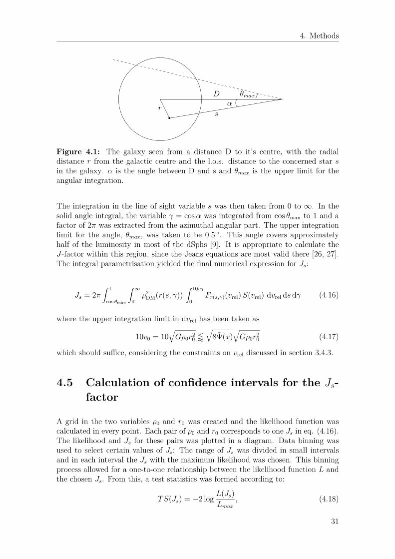
4. Methods
r
D θmaxα
s
Figure 4.1: The galaxy seen from a distance D to it’s centre, with the radialdistance r from the galactic centre and the l.o.s. distance to the concerned star sin the galaxy. α is the angle between D and s and θmax is the upper limit for theangular integration.
The integration in the line of sight variable s was then taken from 0 to ∞. In thesolid angle integral, the variable γ = cosα was integrated from cos θmax to 1 and afactor of 2π was extracted from the azimuthal angular part. The upper integrationlimit for the angle, θmax, was taken to be 0.5 . This angle covers approximatelyhalf of the luminosity in most of the dSphs [9]. It is appropriate to calculate theJ-factor within this region, since the Jeans equations are most valid there [26, 27].The integral parametrisation yielded the final numerical expression for Js:
Js = 2π∫ 1
cos θmax
∫ ∞0
ρ2DM(r(s, γ))
∫ 10v0
0Fr(s,γ)(vrel)S(vrel) dvrel ds dγ (4.16)
where the upper integration limit in dvrel has been taken as
10v0 = 10√Gρ0r2
0 /√
8Ψ(x)√Gρ0r2
0 (4.17)
which should suffice, considering the constraints on vrel discussed in section 3.4.3.
4.5 Calculation of confidence intervals for the Js-factor
A grid in the two variables ρ0 and r0 was created and the likelihood function wascalculated in every point. Each pair of ρ0 and r0 corresponds to one Js in eq. (4.16).The likelihood and Js for these pairs was plotted in a diagram. Data binning wasused to select certain values of Js: The range of Js was divided in small intervalsand in each interval the Js with the maximum likelihood was chosen. This binningprocess allowed for a one-to-one relationship between the likelihood function L andthe chosen Js. From this, a test statistics was formed according to:
TS(Js) = −2 log L(Js)Lmax
, (4.18)
31
4. Methods
where Lmax is the value of the absolute maximum likelihood for any pair ρ0 and r0.The confidence levels were then calculated using the chi-squared distribution withone degree of freedom.
4.6 Validation of method and complementary cal-culations
The validation of our likelihood estimation of Js was made by calculating an like-lihood estimation of the J-factor without self-interaction using the same likelihoodestimation technique and comparing this to Chiappo et. al [9]. The J-factor with-out self-interaction was computed by setting the Sommerfeld enhancement to unity,making the velocity integral equal to 1 in 4.16.
To validate that the calculations of the Sommerfeld enhancement factor S(v) andthe dark matter velocity distribution F (v) are correct, the results was compared toother studies [16, 17]. Also, as a sanity check, the integral of F (v) was evaluatedfor each radial distance from the galactic centre to compare how close this value isto 1.
For further analysis, Js was calculated for constant Sommerfeld enhancement, S(v∗).This is a standard calculation for J-factors accounting self-interaction, for example in[28]. The enhancement becomes constant when considering only the mean velocityof the stars in the galaxy, i.e. no consideration of the distribution of velocities.Typical values for v∗ in dSphs are 10−5 in units of c [21].
32
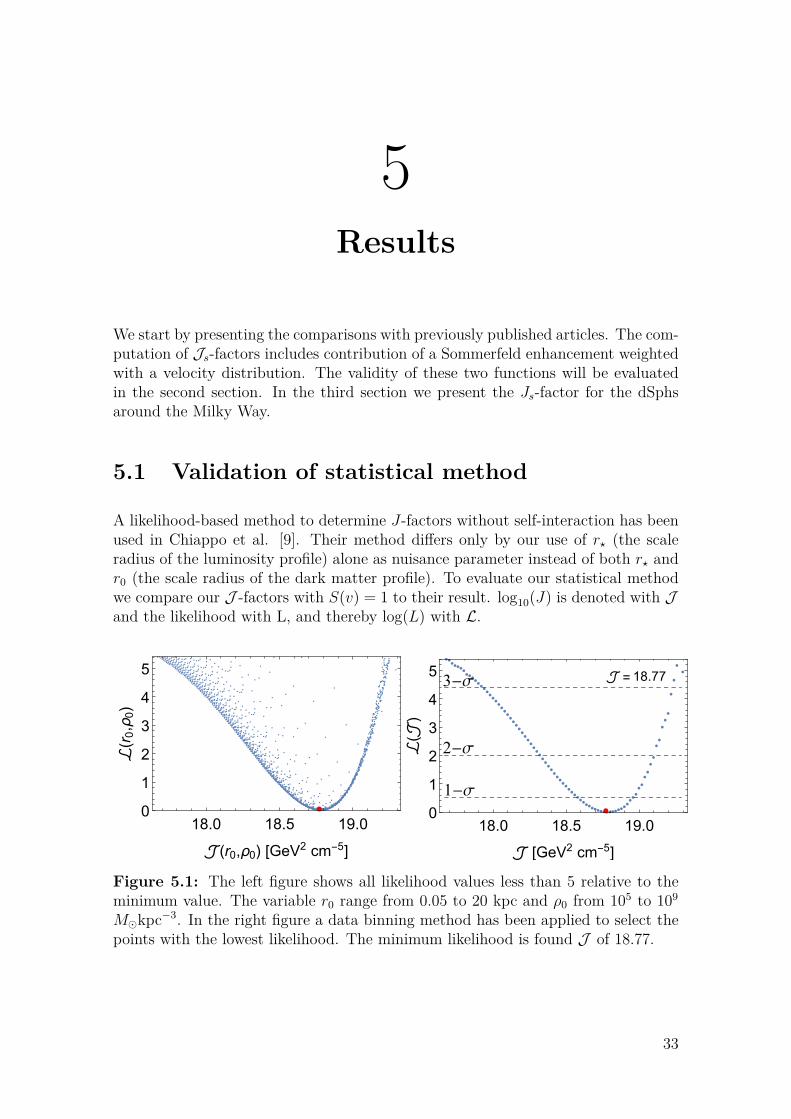
5Results
We start by presenting the comparisons with previously published articles. The com-putation of Js-factors includes contribution of a Sommerfeld enhancement weightedwith a velocity distribution. The validity of these two functions will be evaluatedin the second section. In the third section we present the Js-factor for the dSphsaround the Milky Way.
5.1 Validation of statistical method
A likelihood-based method to determine J-factors without self-interaction has beenused in Chiappo et al. [9]. Their method differs only by our use of r? (the scaleradius of the luminosity profile) alone as nuisance parameter instead of both r? andr0 (the scale radius of the dark matter profile). To evaluate our statistical methodwe compare our J -factors with S(v) = 1 to their result. log10(J) is denoted with Jand the likelihood with L, and thereby log(L) with L.
18.0 18.5 19.00
1
2
3
4
5
r0,ρ0 [GeV2 cm-5]
ℒ(r0,ρ0)
18.773-σ
2-σ
1-σ
18.0 18.5 19.00
1
2
3
4
5
[GeV2 cm-5]
ℒ(
)
Figure 5.1: The left figure shows all likelihood values less than 5 relative to theminimum value. The variable r0 range from 0.05 to 20 kpc and ρ0 from 105 to 109
Mkpc−3. In the right figure a data binning method has been applied to select thepoints with the lowest likelihood. The minimum likelihood is found J of 18.77.
33

5. Results
Table 5.1 shows the discrepancy with Chiappo et al. for 20 dSph. The seven galaxiesabove the dashed line has a J that lies within the 1-σ from the J in Chiappo et al.Our J for Draco differs with 4% and Segue 1 differs with 18% [9]. For four of thegalaxies below the dashed line, the 1-σ intervals overlap. These are Coma Berenices,Canes Venatici II, Bootes II and Ursa Major II. For some of the galaxies one of the1-σ interval limits are not existing due to lack of data points.
Table 5.1: Table comparing J-factors with Chiappo et al. [9]. Galaxies above thedashed line have a J which include the J from [9] within 1-σ. Missing 1-σ-levelsare indicated with “-”. The difference is given as ∆J , the log10 of the ratio betweenour and the referred J-factors. The last three columns are the optimised values forr?, r0 and ρ0.
J ∆J r∗ r0 ρ0
Galaxy [GeV2 cm−5] [kpc] [kpc] [Mkpc−3]Draco 18.77+0.16
−0.19 −0.02 0.21 14.95 1.79 · 106
Leo I 17.70+0.18−0.18 −0.03 0.37 9.90 1.79 · 106
Ursa Major I 17.94+0.64−0.91 −0.09 0.48 0.21 2.26 · 108
Leo IV 16.54+0.82−1.33 −0.19 0.24 0.21 7.39 · 107
Willman 1 19.60+0.37−0.33 −0.26 0.029 17.98 2.60 · 106
Leo T 16.38+1.21−0.72 −0.55 1.86 0.21 1.71 · 108
Segue 1 18.67+0.82−2.37 −0.75 0.085 0.21 1.29 · 108
Sculptor 18.87+0.14− 0.17 0.11 0.61 1.18 · 108
Coma Berenices 19.42+0.22−0.21 0.37 0.0033 1.82 2.92 · 107
Carina 17.52+0.23−0.27 −0.39 0.52 20 3.35 · 105
Canes Venatici II 18.37+0.32−0.27 0.54 0.016 13.13 1.96 · 106
Sagittarius 20.34 −−0.13 0.57 0.079 1.01 1.18 · 108
Bootes II 19.22+0.40−3.33 0.58 0.026 17.78 1.79 · 106
Ursa Major II 19.89+0.24−0.30 0.63 0.0033 2.83 2.42 · 107
Canes Venatici I 18.08 −−0.23 0.75 0.037 0.21 6.28 · 108
Ursa Minor 19.48 −−0.37 0.84 0.024 0.21 9.11 · 108
Fornax 17.09+0.10−0.04 −0.95 1.97 9.50 6.43 · 105
Sextans 18.77+0.08− 1.01 0.05 0.21 5.21 · 108
Bootes I 17.93+0.40−0.45 1.11 0.0044 2.83 4.13 · 106
Hercules 18.50+0.16−0.17 1.17 0.036 20 1.35 · 106
A further investigation of the likelihood on the parameter space r0, ρ0, as in figure5.2, shows a long flat valley for the likelihood. However, the J -factors in fig. 5.1have a similar structure. J gets a well defined maximum likelihood value as seen inthe right of fig. 5.1.
Some error estimations for the galaxies in table 5.1 gives unevaluated 1-σ levels.One such galaxy is Canes Venatici I, seen in fig. 5.3. The left plot is a contour plotover r0 and ρ0, showing the 1,2,3-σ error estimations and J -values. The right plotis the likelihood and J , both calculated in the r0, ρ0-space.
34
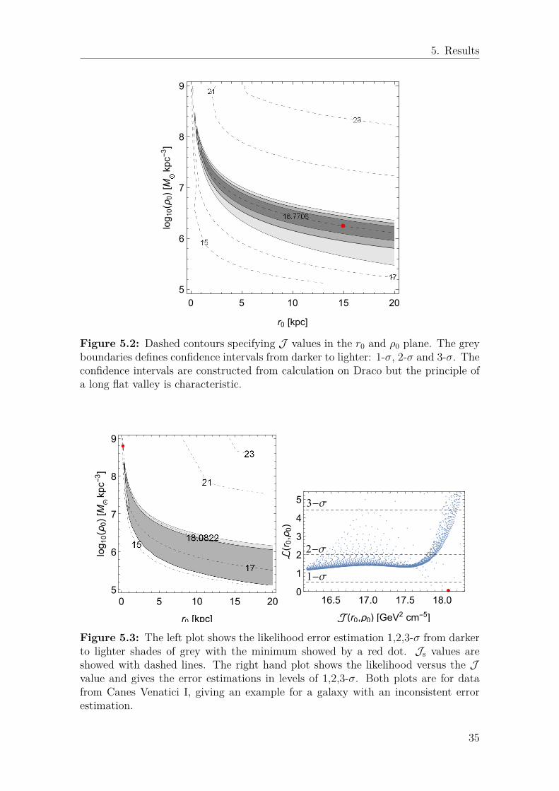
5. Results
17
0 5 10 15 20
5
6
7
8
9
r0 [kpc]
log10(0)[M
kpc-3]
Figure 5.2: Dashed contours specifying J values in the r0 and ρ0 plane. The greyboundaries defines confidence intervals from darker to lighter: 1-σ, 2-σ and 3-σ. Theconfidence intervals are constructed from calculation on Draco but the principle ofa long flat valley is characteristic.
0 5 10 15 205
6
7
8
9
r0 [kpc]
log10(0)[M
kpc-3]
3-σ
2-σ
1-σ
16.5 17.0 17.5 18.00
1
2
3
4
5
r0,ρ0 [GeV2 cm-5]
ℒ(r0,ρ0)
Figure 5.3: The left plot shows the likelihood error estimation 1,2,3-σ from darkerto lighter shades of grey with the minimum showed by a red dot. Js values areshowed with dashed lines. The right hand plot shows the likelihood versus the Jvalue and gives the error estimations in levels of 1,2,3-σ. Both plots are for datafrom Canes Venatici I, giving an example for a galaxy with an inconsistent errorestimation.
35
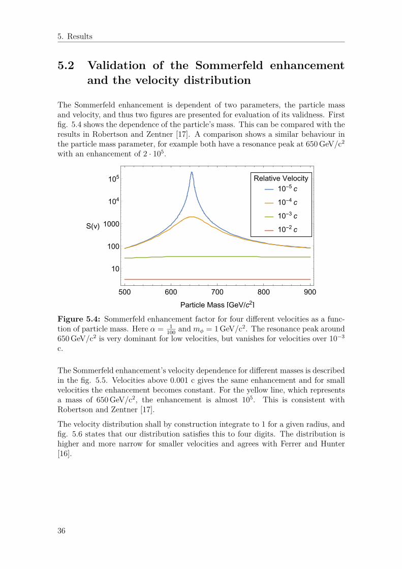
5. Results
5.2 Validation of the Sommerfeld enhancementand the velocity distribution
The Sommerfeld enhancement is dependent of two parameters, the particle massand velocity, and thus two figures are presented for evaluation of its validness. Firstfig. 5.4 shows the dependence of the particle’s mass. This can be compared with theresults in Robertson and Zentner [17]. A comparison shows a similar behaviour inthe particle mass parameter, for example both have a resonance peak at 650 GeV/c2
with an enhancement of 2 · 105.
Relative Velocity
10-5 c
10-4 c
10-3 c
10-2 c
500 600 700 800 900
10
100
1000
104
105
Particle Mass [GeV/c2]
S(v)
Figure 5.4: Sommerfeld enhancement factor for four different velocities as a func-tion of particle mass. Here α = 1
100 and mφ = 1 GeV/c2. The resonance peak around650 GeV/c2 is very dominant for low velocities, but vanishes for velocities over 10−3
c.
The Sommerfeld enhancement’s velocity dependence for different masses is describedin the fig. 5.5. Velocities above 0.001 c gives the same enhancement and for smallvelocities the enhancement becomes constant. For the yellow line, which representsa mass of 650 GeV/c2, the enhancement is almost 105. This is consistent withRobertson and Zentner [17].
The velocity distribution shall by construction integrate to 1 for a given radius, andfig. 5.6 states that our distribution satisfies this to four digits. The distribution ishigher and more narrow for smaller velocities and agrees with Ferrer and Hunter[16].
36
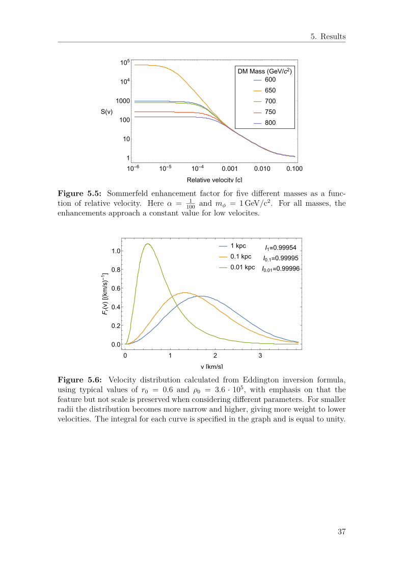
5. Results
DM Mass (GeV/c2)
600
650
700
750
800
10-6 10-5 10-4 0.001 0.010 0.100
1
10
100
1000
104
105
Relative velocity [c]
S(v)
Figure 5.5: Sommerfeld enhancement factor for five different masses as a func-tion of relative velocity. Here α = 1
100 and mφ = 1 GeV/c2. For all masses, theenhancements approach a constant value for low velocites.
1 kpc
0.1 kpc
0.01 kpc
I1=0.99954
I0.1=0.99995
I0.01=0.99996
0 1 2 3
0.0
0.2
0.4
0.6
0.8
1.0
v [km/s]
Fr(v)[(km/s)-1]
Figure 5.6: Velocity distribution calculated from Eddington inversion formula,using typical values of r0 = 0.6 and ρ0 = 3.6 · 105, with emphasis on that thefeature but not scale is preserved when considering different parameters. For smallerradii the distribution becomes more narrow and higher, giving more weight to lowervelocities. The integral for each curve is specified in the graph and is equal to unity.
37
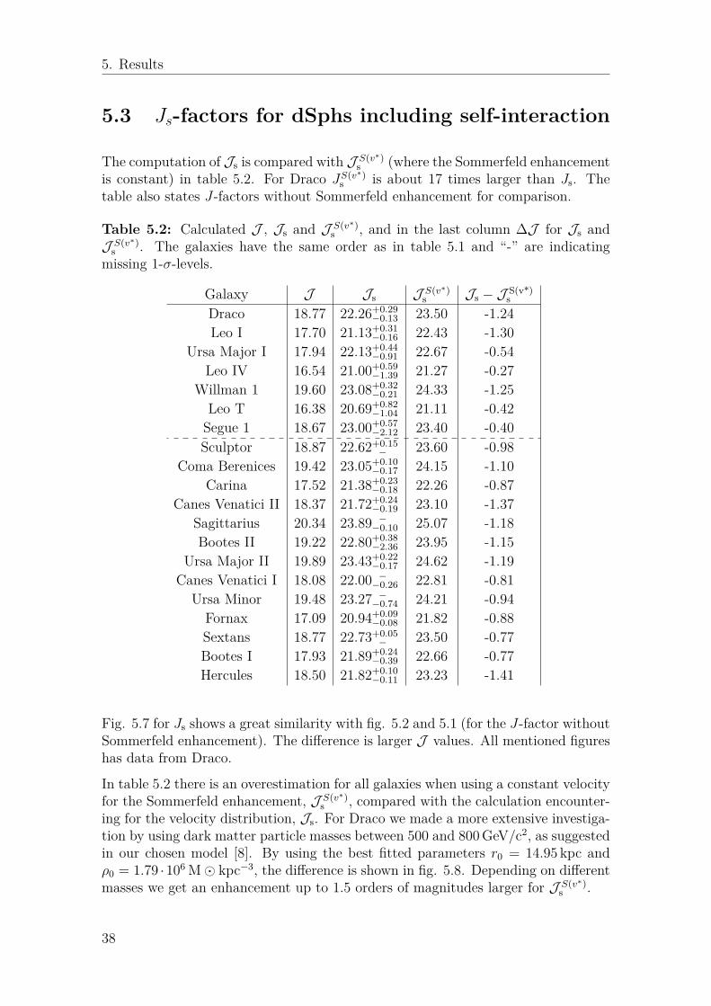
5. Results
5.3 Js-factors for dSphs including self-interaction
The computation of Js is compared with J S(v∗)s (where the Sommerfeld enhancement
is constant) in table 5.2. For Draco JS(v∗)s is about 17 times larger than Js. The
table also states J-factors without Sommerfeld enhancement for comparison.
Table 5.2: Calculated J , Js and J S(v∗)s , and in the last column ∆J for Js and
J S(v∗)s . The galaxies have the same order as in table 5.1 and “-” are indicating
missing 1-σ-levels.
Galaxy J Js J S(v∗)s Js − J S(v*)
sDraco 18.77 22.26+0.29
−0.13 23.50 -1.24Leo I 17.70 21.13+0.31
−0.16 22.43 -1.30Ursa Major I 17.94 22.13+0.44
−0.91 22.67 -0.54Leo IV 16.54 21.00+0.59
−1.39 21.27 -0.27Willman 1 19.60 23.08+0.32
−0.21 24.33 -1.25Leo T 16.38 20.69+0.82
−1.04 21.11 -0.42Segue 1 18.67 23.00+0.57
−2.12 23.40 -0.40Sculptor 18.87 22.62+0.15
− 23.60 -0.98Coma Berenices 19.42 23.05+0.10
−0.17 24.15 -1.10Carina 17.52 21.38+0.23
−0.18 22.26 -0.87Canes Venatici II 18.37 21.72+0.24
−0.19 23.10 -1.37Sagittarius 20.34 23.89 −−0.10 25.07 -1.18Bootes II 19.22 22.80+0.38
−2.36 23.95 -1.15Ursa Major II 19.89 23.43+0.22
−0.17 24.62 -1.19Canes Venatici I 18.08 22.00 −−0.26 22.81 -0.81
Ursa Minor 19.48 23.27 −−0.74 24.21 -0.94Fornax 17.09 20.94+0.09
−0.08 21.82 -0.88Sextans 18.77 22.73+0.05
− 23.50 -0.77Bootes I 17.93 21.89+0.24
−0.39 22.66 -0.77Hercules 18.50 21.82+0.10
−0.11 23.23 -1.41
Fig. 5.7 for Js shows a great similarity with fig. 5.2 and 5.1 (for the J-factor withoutSommerfeld enhancement). The difference is larger J values. All mentioned figureshas data from Draco.
In table 5.2 there is an overestimation for all galaxies when using a constant velocityfor the Sommerfeld enhancement, J S(v∗)
s , compared with the calculation encounter-ing for the velocity distribution, Js. For Draco we made a more extensive investiga-tion by using dark matter particle masses between 500 and 800 GeV/c2, as suggestedin our chosen model [8]. By using the best fitted parameters r0 = 14.95 kpc andρ0 = 1.79 ·106 M kpc−3, the difference is shown in fig. 5.8. Depending on differentmasses we get an enhancement up to 1.5 orders of magnitudes larger for J S(v∗)
s .
38
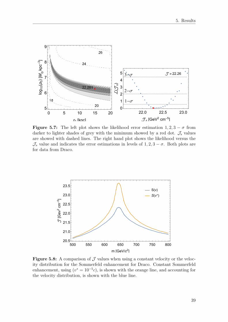
5. Results
20
0 5 10 15 205
6
7
8
9
r0 [kpc]
log10(0)[M
kpc-3]
3-σ
2-σ
1-σ
22.26
22.0 22.5 23.0
0
1
2
3
4
5
s [GeV2cm
-5]ℒ(
s)
Figure 5.7: The left plot shows the likelihood error estimation 1, 2, 3 − σ fromdarker to lighter shades of grey with the minimum showed by a red dot. Js valuesare showed with dashed lines. The right hand plot shows the likelihood versus theJs value and indicates the error estimations in levels of 1, 2, 3 − σ. Both plots arefor data from Draco.
S(v)
S(v*)
500 550 600 650 700 750 800
20.5
21.0
21.5
22.0
22.5
23.0
23.5
m [GeV/c2]
[Gev2cm
-5]
Figure 5.8: A comparison of J values when using a constant velocity or the veloc-ity distribution for the Sommerfeld enhancement for Draco. Constant Sommerfeldenhancement, using (v∗ = 10−5c), is shown with the orange line, and accounting forthe velocity distribution, is shown with the blue line.
39
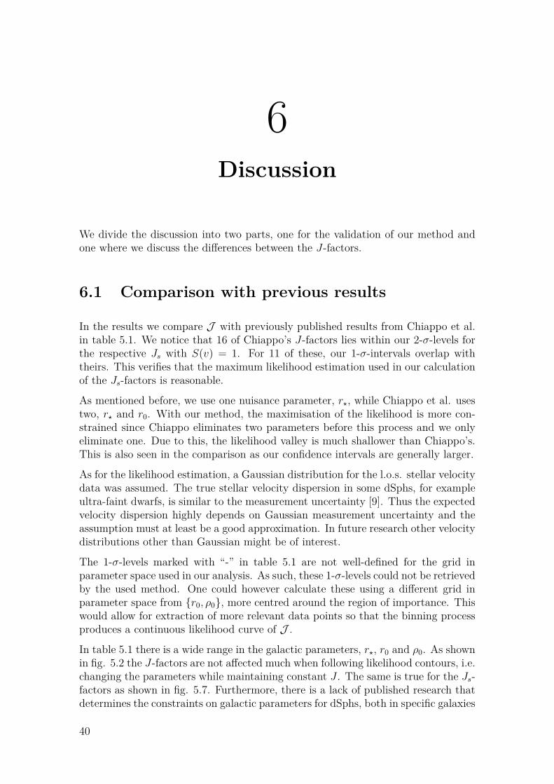
6Discussion
We divide the discussion into two parts, one for the validation of our method andone where we discuss the differences between the J-factors.
6.1 Comparison with previous results
In the results we compare J with previously published results from Chiappo et al.in table 5.1. We notice that 16 of Chiappo’s J-factors lies within our 2-σ-levels forthe respective Js with S(v) = 1. For 11 of these, our 1-σ-intervals overlap withtheirs. This verifies that the maximum likelihood estimation used in our calculationof the Js-factors is reasonable.
As mentioned before, we use one nuisance parameter, r?, while Chiappo et al. usestwo, r? and r0. With our method, the maximisation of the likelihood is more con-strained since Chiappo eliminates two parameters before this process and we onlyeliminate one. Due to this, the likelihood valley is much shallower than Chiappo’s.This is also seen in the comparison as our confidence intervals are generally larger.
As for the likelihood estimation, a Gaussian distribution for the l.o.s. stellar velocitydata was assumed. The true stellar velocity dispersion in some dSphs, for exampleultra-faint dwarfs, is similar to the measurement uncertainty [9]. Thus the expectedvelocity dispersion highly depends on Gaussian measurement uncertainty and theassumption must at least be a good approximation. In future research other velocitydistributions other than Gaussian might be of interest.
The 1-σ-levels marked with “-” in table 5.1 are not well-defined for the grid inparameter space used in our analysis. As such, these 1-σ-levels could not be retrievedby the used method. One could however calculate these using a different grid inparameter space from r0, ρ0, more centred around the region of importance. Thiswould allow for extraction of more relevant data points so that the binning processproduces a continuous likelihood curve of J .
In table 5.1 there is a wide range in the galactic parameters, r?, r0 and ρ0. As shownin fig. 5.2 the J-factors are not affected much when following likelihood contours, i.e.changing the parameters while maintaining constant J . The same is true for the Js-factors as shown in fig. 5.7. Furthermore, there is a lack of published research thatdetermines the constraints on galactic parameters for dSphs, both in specific galaxies
40

6. Discussion
and generally. Such research could be of interest, especially for those galaxies withunidentified 1-σ levels. These constraints can be used to focus the analysis on acertain parameter range and increase the amount of likelihood estimations aroundthe maximum likelihood in the data in fig. 5.3. The data binning will then be morecompatible with a 1-σ level determination.
6.2 The impact of a proper velocity distribution
We have studied the generalised J-factor in different situations. The classical ap-proach without self-interaction has been extensively covered in the last section withcomparisons to previous research. Here, we compare the rigorous Js-factor to thepreviously used approximation of a constant Sommerfeld enhancement factor toevaluate the differences from when one uses a proper velocity distribution [28].
As shown in table 5.2 there is a significant increase of 3 to 4 orders of magnitude(depending on which galaxy) in the J-factor when introducing self-interaction. Anincrease in the factor is of course expected as the Sommerfeld enhancement factor foran attractive potential is always 1 or larger, but this fact does not fully explain thedifference of 3 to 4 orders of magnitude. It can however be explained by the chosendark matter particle mass used in the analysis. We have assumed a particle mass of650 GeV/c2 which, as can be seen in fig. 5.4, corresponds to a resonance peak withsignificantly higher Sommerfeld enhancement values. This resonance peak couldbe a factor of great importance in future indirect dark matter searches, as a veryhigh observed gamma ray flux could indicate dark matter masses in the region ofa resonance peak. On the other hand, outside the resonance peaks the Sommerfeldenhancements for different masses quickly reaches fairly similar values, and as such,determining a hypothetical dark matter mass in those regions might be significantlyharder.
Whether one should include the velocity distribution or not when calculating Jsis due to two aspects, namely which particle mass and which galactic parameters(r0 and ρ0) that is of interest. Particle masses in a resonance peak gives a largeoverestimation of J S(v∗)
s as shown in fig. 5.8. However, one can see in the samefigure that if particle masses far away from resonance peaks are of interest thetwo calculations are almost equal. Furthermore, in fig. 5.5 one can see that theSommerfeld enhancement becomes constant for low speeds, from 10−4 c to 10−5 cdependent on particle mass. So if no higher speeds are of consideration there will beno need to perform the Js with the velocity distribution. This is the case for smallgalaxy radii, where the velocity is lower, as seen in fig. 5.6.
41

7Conclusion
In this thesis we present an ab initio approach to calculate a more general J-factorfor dwarf spheroidal galaxies. This generalisation takes self-interaction between darkmatter particles into account in a more rigorous manner than before.
We can conclude that if dark matter particles has the properties of self-interaction,the J-factors significantly increases from 1017−1020 to 1021−1024 for dwarf spheroidalgalaxies. Furthermore, we conclude that the standard approximative calculation,using a constant Sommerfeld enhancement, overestimated the Js-factor of up to 1.5orders of magnitude.
We verify that the maximum likelihood estimation used in our calculation of theJs-factors is reasonable. By comparison with calculations of J-factors without self-interaction, the confidence intervals are larger. This is due to the inevitable con-straints appearing in the parameter space when considering self-interaction.
During the completion of this thesis another report with a similar purpose wasuploaded on arXiv.org, [29]. An important difference between our studies lies in thesolution of the Schrödinger equation including a Yukawa potential. They use anapproximation allowing an analytical solution of the Schrödinger equation. We usea numerical approach to solve the full Schrödinger equation. Our method introducesnumerical difficulties but gives more accurate results.
42
References
[1] M. Ackermann et al., “Dark matter constraints from observations of 25 milkyway satellite galaxies with the fermi large area telescope”, Physical Review D89 (2014).
[2] G. Bertone and D. Hooper, “A history of dark matter”, (2016).[3] D. D. R. Williams, Planetary fact sheet, NASA Space Data Coordinated Archive,
(Dec. 2016) https://nssdc.gsfc.nasa.gov/planetary/factsheet/.[4] M. Milgrom, “The mond paradigm”, (2008).[5] D. Clowe, A. Gonzalez, and M. Markevitch, “Weak-Lensing Mass Reconstruc-
tion of the Interacting Cluster 1E 0657-558: Direct Evidence for the Existenceof Dark Matter”, Astrophysical Journal 604, 596 (2004).
[6] M. H. Jones, R. J. Lambourne, S. Serjeant, and O. University, An introductionto galaxies and cosmology, 2nd edition (Cambridge University Press, Cam-bridge, 2015).
[7] M. Kamionkowski, “Wimp and axion dark matter”, (1997).[8] N. Arkani-Hamed, D. P. Finkbeiner, T. R. Slatyer, and N. Weiner, “A theory
of dark matter”, Phys. Rev. D 79, 015014 (2009).[9] A. Chiappo et al., “Dwarf spheroidal j-factors without priors: a likelihood-
based analysis for indirect dark matter searches”, Monthly Notices of the RoyalAstronomical Society 466, 669 (2016).
[10] L. Hui, “Unitarity bounds and the cuspy halo problem”, Physical Review Let-ters 86, 3467 (2001).
[11] A. Loeb and N. Weiner, “Cores in dwarf galaxies from dark matter with ayukawa potential”, Physical Review Letters 106, 171302 (2011).
[12] A. Geringer-Sameth et al., “Indication of gamma-ray emission from the newlydiscovered dwarf galaxy reticulum ii”, PHYSICAL REVIEW LETTERS 115,081101 (2015).
[13] D. Harvey et al., “The non-gravitational interactions of dark matter in collidinggalaxy clusters”, (2015).
[14] R. G. Dubinski John; Carlberg, “The structure of cold dark matter halos”,Astrophys.J (1991).
[15] D. N. Spergel and P. J. Steinhardt, “Observational evidence for self-interactingcold dark matter”, Physical Review Letters (1999).
[16] F. Ferrer and D. R. Hunter, “The impact of the phase-space density on theindirect detection of dark matter”, Journal of Cosmology and AstroparticlePhysics 2013 (2013).
43
References
[17] A. R. Z. Brant E. Robertson, “Dark matter annihilation rates with velocity-dependent annihilation cross sections”, Phys. Rev. D (2009).
[18] J. Binney and S. Tremaine, Galactic dynamics (Princeton University Press,Princeton, New Jersey, 1987).
[19] K. S. Krane, Introductory nuclear physics, 2nd ed. (John Wiley & Sons, Inc.,1988).
[20] J. J. Sakurai and J. Napolitano, Modern quantum mechanics, 2nd edition,Pearson new international (Pearson, Harlow, 2014).
[21] R. Iengo, “Sommerfeld enhancement: general results from field theory dia-grams”, Journal of High Energy Physics 2009, 024 (2009).
[22] L. Landau and E. Lifshitz, Quantum mechanics: non-relativistic theory (Perg-amon Press, 1965).
[23] H. C. Plummer, “On the problem of distribution in globular star clusters”,Monthly Notices of the RAS 71, 460 (1911).
[24] H. Zhao, “Analytical models for galactic nuclei”, Monthly Notices of the RoyalAstronomical Society 278, 488 (1996).
[25] J. F. Navarro, C. S. Frenk, and S. D. M. White, “A universal density profilefrom hierarchical clustering”, The Astrophysical Journal 490, 493 (1997).
[26] J. Wolf et al., “Accurate masses for dispersion-supported galaxies”, MonthlyNotices of the Royal Astronomical Society 406, 1220 (2010).
[27] M. G. Walker et al., “Dark matter in the classical dwarf spheroidal galaxies: arobust constraint on the astrophysical factor for gamma-ray flux calculations”,The Astrophysical Journal Letters 733, L46 (2011).
[28] M.-H. Chan, “Does the gamma-ray signal from the central milky way indicatesommerfeld enhancement of dark matter annihilation”, (2016).
[29] K. K. Boddy, J. Kumar, L. E. Strigari, and M.-Y. Wang, “Sommerfeld-enhancedj-factors for dwarf spheroidal galaxies”, (2017).
44
AMathematica code
Here we present the Mathematica code used in the project.
I
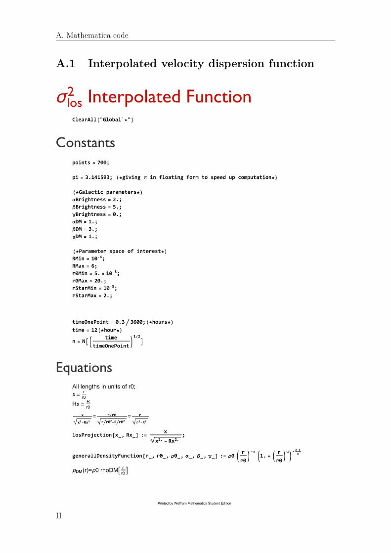
σlos2 Interpolated FunctionClearAll["Global`*"]
Constantspoints = 700;
pi = 3.141593; (*giving π in floating form to speed up computation*)
(*Galactic parameters*)
αBrightness = 2.;
βBrightness = 5.;
γBrightness = 0.;
αDM = 1.;
βDM = 3.;
γDM = 1.;
(*Parameter space of interest*)
RMin = 10-4;
RMax = 6;
r0Min = 5. * 10-3;
r0Max = 20.;
rStarMin = 10-3;
rStarMax = 2.;
timeOnePoint = 0.3 3600;(*hours*)
time = 12(*hour*)
n = Ntime
timeOnePoint
1/2
EquationsAll lengths in units of r0;x =
r
r0
Rx =R
r0
x
x2-Rx2= r/r0
rr02-Rr02= r
r2-R2
losProjection[x_, Rx_] :=x
x2. - Rx2.;
generallDensityFunction[r_, r0_, ρ0_, α_, β_, γ_] := ρ0 r
r0-γ
1. + r
r0α
-
β-γ
α
ρDM(r)=ρ0 rhoDMr
r0
Printed by Wolfram Mathematica Student Edition
A. Mathematica code
A.1 Interpolated velocity dispersion function
II
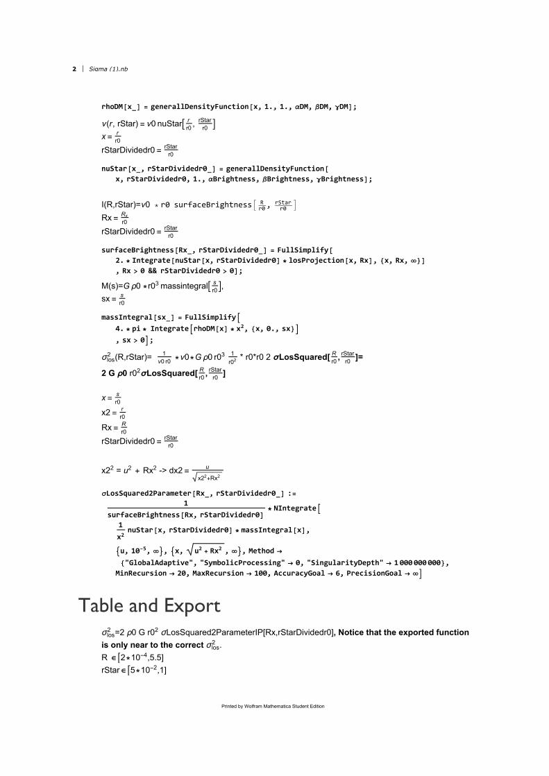
rhoDM[x_] = generallDensityFunction[x, 1., 1., αDM, βDM, γDM];
ν(r, rStar) = ν0 nuStar rr0
, rStarr0
x =r
r0
rStarDividedr0 =rStar
r0
nuStar[x_, rStarDividedr0_] = generallDensityFunction[
x, rStarDividedr0, 1., αBrightness, βBrightness, γBrightness];
I(R,rStar)=ν0 * r0 surfaceBrightness Rr0, rStar
r0
Rx =Rx
r0
rStarDividedr0 =rStar
r0
surfaceBrightness[Rx_, rStarDividedr0_] = FullSimplify[
2. * Integrate[nuStar[x, rStarDividedr0] * losProjection[x, Rx], x, Rx, ∞]
, Rx > 0 && rStarDividedr0 > 0];
M(s)=G ρ0 * r03 massintegral sr0,
sx =s
r0
massIntegral[sx_] = FullSimplify
4. * pi * IntegraterhoDM[x] * x2, x, 0., sx
, sx > 0;
σlos2 (R,rStar)= 1
ν0 r0 *ν0*G ρ0 r03 1
r02 * r0*r0 2 σLosSquared[ Rr0
, rStarr0
]=
2 G ρ0 r02σLosSquared[ Rr0
, rStarr0
]
x =s
r0
x2 =r
r0
Rx =R
r0
rStarDividedr0 =rStar
r0
x22 = u2 + Rx2 -> dx2 =u
x22+Rx2
σLosSquared2Parameter[Rx_, rStarDividedr0_] :=
1
surfaceBrightness[Rx, rStarDividedr0]* NIntegrate
1
x2nuStar[x, rStarDividedr0] * massIntegral[x],
u, 10-5, ∞, x, u2 + Rx2 , ∞, Method →
"GlobalAdaptive", "SymbolicProcessing" → 0, "SingularityDepth" → 1 000 000 000,
MinRecursion → 20, MaxRecursion → 100, AccuracyGoal → 6, PrecisionGoal → ∞
Table and Exportσlos
2 =2 ρ0 G r02 σLosSquared2ParameterIP[Rx,rStarDividedr0], Notice that the exported function
is only near to the correct σlos2 .
R ∈ 2*10-4,5.5]
rStar ∈ 5*10-2,1]
2 Sigma (1).nb
Printed by Wolfram Mathematica Student Edition

r0 ∈ 5*10-2,10]
points = 700;
RxMin =RMin
r0Max;
RxMax =RMax
r0Min;
rStarDividedr0Min =rStarMin
r0Max;
rStarDividedr0Max =rStarMax
r0Min;
stepSizeRx =RxMax1/10 - RxMin1/10
points - 1;
stepSizerStarDividedr0 =rStarDividedr0Max1/10 - rStarDividedr0Min1/10
points - 1;
σTableNFW =
ParallelTable
Rx10, rStarDividedr010, σLosSquared2ParameterRx10, rStarDividedr010,
Rx, RxMin1/10, RxMax1/10, stepSizeRx,
rStarDividedr0, rStarDividedr0Min1/10,
rStarDividedr0Max1/10, stepSizerStarDividedr0;
SetDirectory[NotebookDirectory[]];
Flatten[σTableNFW, 1] >> "σTableNFW_700"
Sigma (1).nb 3
Printed by Wolfram Mathematica Student Edition
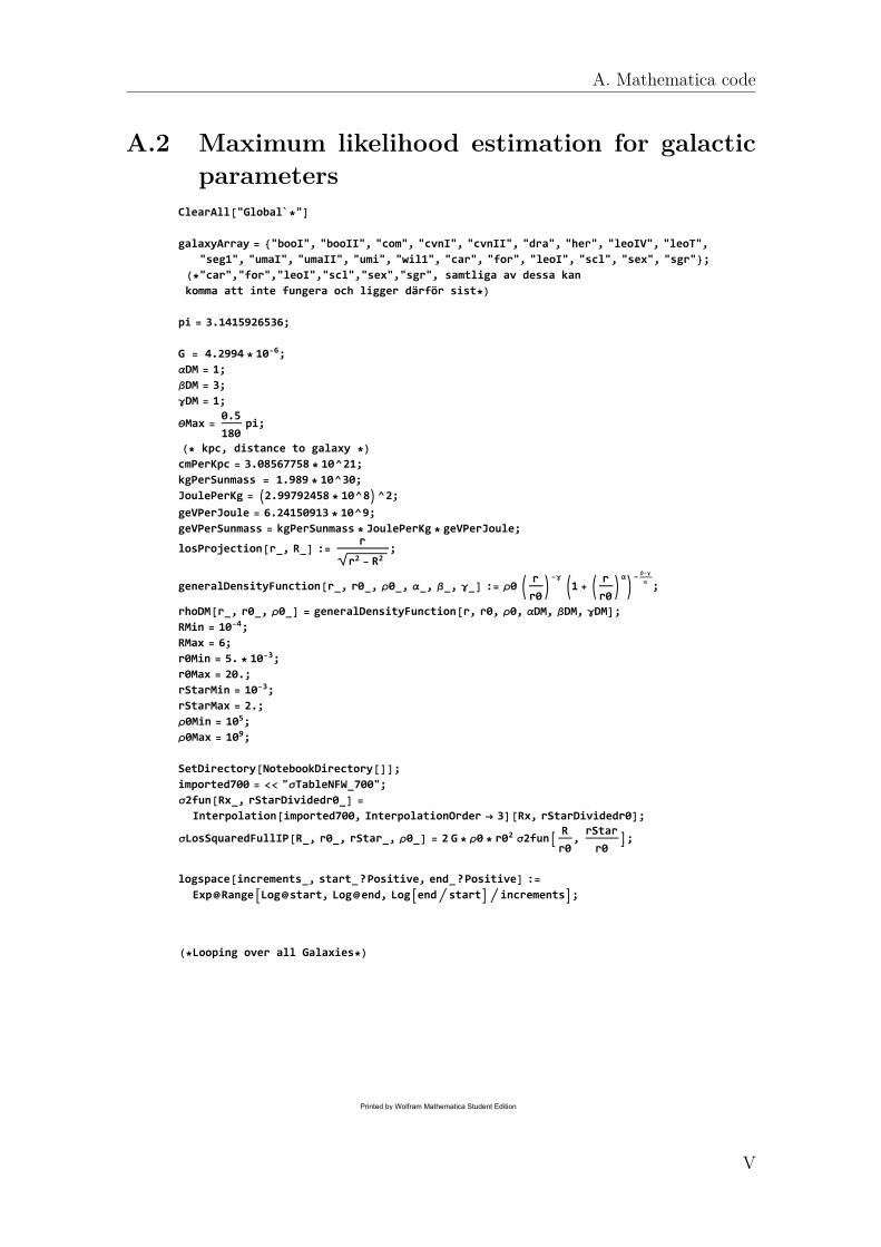
ClearAll["Global`*"]
galaxyArray = "booI", "booII", "com", "cvnI", "cvnII", "dra", "her", "leoIV", "leoT",
"seg1", "umaI", "umaII", "umi", "wil1", "car", "for", "leoI", "scl", "sex", "sgr";
(*"car","for","leoI","scl","sex","sgr", samtliga av dessa kan
komma att inte fungera och ligger därför sist*)
pi = 3.1415926536;
G = 4.2994 * 10-6;
αDM = 1;
βDM = 3;
γDM = 1;
θMax =0.5
180pi;
(* kpc, distance to galaxy *)
cmPerKpc = 3.08567758 * 10^21;
kgPerSunmass = 1.989 * 10^30;
JoulePerKg = 2.99792458 * 10^8^2;
geVPerJoule = 6.24150913 * 10^9;
geVPerSunmass = kgPerSunmass * JoulePerKg * geVPerJoule;
losProjection[r_, R_] :=r
r2 - R2;
generalDensityFunction[r_, r0_, ρ0_, α_, β_, γ_] := ρ0 r
r0-γ
1 + r
r0α
-
β-γ
α
;
rhoDM[r_, r0_, ρ0_] = generalDensityFunction[r, r0, ρ0, αDM, βDM, γDM];
RMin = 10-4;
RMax = 6;
r0Min = 5. * 10-3;
r0Max = 20.;
rStarMin = 10-3;
rStarMax = 2.;
ρ0Min = 105;
ρ0Max = 109;
SetDirectory[NotebookDirectory[]];
imported700 = << "σTableNFW_700";
σ2fun[Rx_, rStarDividedr0_] =
Interpolation[imported700, InterpolationOrder → 3][Rx, rStarDividedr0];
σLosSquaredFullIP[R_, r0_, rStar_, ρ0_] = 2 G * ρ0 * r02 σ2funR
r0,rStar
r0;
logspace[increments_, start_?Positive, end_?Positive] :=
Exp@RangeLog@start, Log@end, Logend start increments;
(*Looping over all Galaxies*)
Printed by Wolfram Mathematica Student Edition
A. Mathematica code
A.2 Maximum likelihood estimation for galacticparameters
V
Fori = 1, i ≤ Length[galaxyArray], i++,
ClearAll[galaxy, distance, tableGalaxie, σLosSquaredRList,
r0rStarρ0MinimizeFunction, r0rStarρ0MinimizeFunctionConst,
minimizerStar, tableρ0r0WithTime, time, tableρ0r0, tableJ];
galaxy = galaxyArray[[i]];
SetDirectory[NotebookDirectory[]];
SetDirectory["allVelocites"];
tableGalaxy = Import[ToString@StringForm["velocities_``.dat", galaxy], "Table"];
vLosR = Abs[tableGalaxy[[All, 2]]];
vLosRMean = Mean[vLosR];
σLosSquaredRList[r0_, rStar_, ρ0_] =
tableGalaxy[[All, 3]]2+ σLosSquaredFullIP[tableGalaxy[[All, 1]], r0, rStar, ρ0];
r0rStarρ0MinimizeFunction[r0_, rStar_, ρ0_] = Total
(vLosR - vLosRMean)2
σLosSquaredRList[r0, rStar, ρ0]+ Log[2. pi * σLosSquaredRList[r0, rStar, ρ0]];
r0rStarρ0MinimizeFunctionConst[r0_?NumericQ, rStar_?NumericQ, ρ0_?NumericQ] =
Piecewise
10.10., rStar ≤ rStarMin, galaxy = "scl";
r0rStarρ0MinimizeFunction[r0, rStar, ρ0], rStar ≥ rStarMin && rStar ≤ rStarMax,
10.10., rStar ≥ rStarMax
;
minimizerStar[r0_?NumericQ, ρ0_?NumericQ] :=
FindMinimum[r0rStarρ0MinimizeFunctionConst[r0, rStar, ρ0],
rStar, 0.1, 0.1 + 0.01, Method → "PrincipalAxis", WorkingPrecision → 10];
r0Points = 7;
ρ0Points = 7;
r0Range = N@Ranger0Min, r0Max, r0Max - r0Min r0Points;
ρ0Range = N@logspace[ρ0Points, ρ0Min, ρ0Max];
r0ρ0rStarL = Table[r0, ρ0, rStar /. minimizerStar[r0, ρ0][[2]],
minimizerStar[r0, ρ0][[1]], r0, r0Range, ρ0, ρ0Range];
refinedr0ρ0rStarL = Select[
Flatten[r0ρ0rStarL, 1],
rStarMin + 0.001 < #[[1]][[3]] < rStarMax - 0.001 &
];
SetDirectory[NotebookDirectory[]]
Put[refinedr0ρ0rStarL, ToString[galaxy] <> "_r0ρ0rStarL"]
2 liklihood.nb
Printed by Wolfram Mathematica Student Edition

Old J ClearAll["Global`*"]
Profile constantsαDM = 1;
βDM = 3;
γDM = 1;
Units constants & constants(* kpc, distance to galaxy *)
cmPerKpc = 3.08567758 * 10^21.;
kgPerSunmass = 1.989 * 10^30.;
JoulePerKg = 2.99792458 * 10^8^2.;
geVPerJoule = 6.24150913 * 10^9.;
geVPerSunmass = kgPerSunmass * JoulePerKg * geVPerJoule;
pi = 3.14159265;
particelMass = 600;
G = 4.2994 * 10-6;
Calculating J for a galaxy
Defining galaxygalaxyArray = "booI", "booII", "com", "cvnI", "cvnII", "dra", "her", "leoIV", "leoT",
"seg1", "umaI", "umaII", "umi", "wil1", "car", "for", "leoI", "scl", "sex", "sgr";
(*"car","for","leoI","scl","sex","sgr", samtliga av dessa kan
komma att inte fungera och ligger därför sist*)
Printed by Wolfram Mathematica Student Edition
A. Mathematica code
A.3 Calculate J-factors
VII
Defining J
generalDensityFunction[r_, r0_, ρ0_, α_, β_, γ_] := ρ0 r
r0-γ
1. + r
r0α
-
β-γ
α
;
rhoDM[r_, r0_, ρ0_] = generalDensityFunction[r, r0, ρ0, αDM, βDM, γDM];
θMax =0.5
180.pi;
◼ Get and interpolate p[vrel,x] and S[vrel]Fori = 1, i ≤ Length[galaxyArray], i++,
ClearALL[galaxy, distance, radiusFunction, r0ρ0rStarL, r0ρ0, JOld, Jold];
galaxy = galaxyArray[[i]];
SetDirectory[NotebookDirectory[]];
SetDirectory["Params"];
distance = Import[ToString@StringForm["params_``.dat", galaxy], "Table"][[2]][[1]];
radiusFunction[s_, x_] = distance^2. + s^2. - 2. s distance x ;
JOld[r0_, ρ0_] := Log10
geVPerSunmass^2. * cmPerKpc^-5. *
2. pi *
NIntegrate
rhoDM[radiusFunction[s, x], r0, ρ0]2,
s, 0, ∞, x, Cos[θMax], 1
;
SetDirectory[NotebookDirectory[]];
SetDirectory["Minimasation"];
r0ρ0rStarL = Get[ToString@galaxy <> "_r0ρ0rStarL"];
r0ρ0 = Transpose[r0ρ0rStarL[[All, 1]][[All, 1]], r0ρ0rStarL[[All, 1]][[All, 2]]];
Jold = Parallelize[JOld @@@ r0ρ0];
SetDirectory[NotebookDirectory[]];
Put[Jold, ToString@galaxy <> "_Jold"]
2 J_old.nb
Printed by Wolfram Mathematica Student Edition
Eddington Inversion
ClearAll["Global`*"]
pi = 3.141593;
αDM = 1.;
βDM = 3.;
γDM = 1.;
generalDensityFunction[r_, r0_, ρ0_, α_, β_, γ_] := ρ0 r
r0-γ
1 + r
r0α
-
β-γ
α
rhoDM[x_] = generalDensityFunction[x, 1., 1., αDM, βDM, γDM];
(*ρ0*)
psi[x_] = 4. * pi * FullSimplify
1
x* Integrates2 * rhoDM[s], s, 0., x + Integrate[s * rhoDM[s], s, x, ∞]
, x ≥ 0;
epsilonMax = Limit[psi[x], x → 0];
(*G ρ0 r02*)
Sqrt[8 * Limit[psi[x], x → 0]]
10.0265
rhoDMD[x] = FullSimplify[
D[rhoDM[x], x]
];
(*1
r0ρ0*)
rhoDMD2[x] = FullSimplify[
D[rhoDM[x], x, 2]
];
(*1
r02ρ0*)
psiD[x] = FullSimplify[
D[psi[x], x]
];
(*G ρ0 r0*)
psiD2[x] = FullSimplify[
D[psi[x], x, 2]
];
(*G ρ0*)
integrandEpsilonDistributionFunction[ϵ_?NumericQ, x_?NumericQ] =
rhoDMD[x] * psiD2[x] * psiD[x]-2 - rhoDMD2[x] * psiD[x]-1
Sqrt[ϵ - psi[x]];
(*"1
r0ρ0*G ρ0*
1
G ρ0 r02-
1
r02ρ0*
1
G ρ0 r0
G ρ0 r02"*)
(*1
r03G G ρ0 r02*)
Printed by Wolfram Mathematica Student Edition
A. Mathematica code
A.4 Dark matter velocity distribution in dSphs
IX

Clear[epsilonDistributionFunction]
epsilonDistributionFunction[ϵ_?NumericQ] :=
ReleaseHold
ReplaceAll[
Evaluate[
Flatten@NSolve[psi[xmin] ⩵ ϵ && xmin ≥ 0, xmin]
]
]
Hold
1
8. pi2* NIntegrate[integrandEpsilonDistributionFunction[ϵ, x], x, xmin, ∞,
Method → "GlobalAdaptive", "SymbolicProcessing" → 0, "SingularityDepth" →
10 000, MinRecursion → 10 000, MaxRecursion → 100 000, AccuracyGoal → 5]
;
(*" 1
r03G G ρ0 r02*r0"*)
(*1
r02G Gρ0r02*)
epsilonDistributionFunctionTable1 = Tableϵ10., epsilonDistributionFunctionϵ10.,
ϵ, 10.-6.1./10.
, 1.1./10.,1.1./10. - 10.-6.1./10.
100. // Timing
epsilonDistributionFunctionTable2 = Tableϵ, epsilonDistributionFunction[ϵ],
ϵ, 1., 10., 10. 100.
epsilonDistributionFunctionTable3 = Tableϵ, epsilonDistributionFunction[ϵ],
ϵ, 10., epsilonMax - 1. 2.,epsilonMax - 10.-2. - 10.
100.
epsilonDistributionFunctionTable4 = Tableϵ, epsilonDistributionFunction[ϵ],
ϵ, epsilonMax - 1. 2., epsilonMax - 10.-7.,
epsilonMax - 10.-7. - epsilonMax - 1. 2.
7000.
epsilonDistributionFunctionTable =
Join[epsilonDistributionFunctionTable1, epsilonDistributionFunctionTable2,
epsilonDistributionFunctionTable3, epsilonDistributionFunctionTable4];
SetDirectory[NotebookDirectory[]];
epsilonDistributionFunctionTable >> "f(ϵ)Table";
SetDirectory[NotebookDirectory[]];
epsilonDistributionFunctionTable = DeleteDuplicates[Get["fofepsilon"]];
epsilonDistributionFunctionIP = Interpolation[Re[epsilonDistributionFunctionTable]]
(*control f(ϵ)*)
Plot[Log[epsilonDistributionFunctionIP[ϵ]], ϵ, 0, epsilonMax]
2 edington complited.nb
Printed by Wolfram Mathematica Student Edition
RelativVelocety Distribution
◼ Limits
(*[v]= Gρ0r02 *)
(*[psi[x]]= Gρ0r02 *)
upperLimitVelocityIntegral1[vRel_, x_] := 2. psi[x] -vRel
2.;
lowerLimitVelocityIntegral1 = 0.;
upperLimitZIntegral1 = 1.;
lowerLimitZIntegral1 = 0.;
upperLimitVelocityIntegral2[vRel_, x_] :=8. psi[x] - vRel2.
2.;
lowerLimitVelocityIntegral2[vRel_, x_] := upperLimitVelocityIntegral1[vRel, x];
upperLimitZIntegral2[vRel_, vCM_?NumericQ, x_] =8. psi[x] - vRel2. - 4. * vCM2.
4. * vCM * vRel;
lowerLimitZIntegral2 = 0.;
relativeVelocityϵNegative[vRel_?NumericQ, x_?NumericQ, vCM_?NumericQ, z_?NumericQ] =
psi[x] -vCM2.
2.-vRel2.
8.-vCM * vRel * z
2.;
relativeVelocityϵPositive[vRel_?NumericQ, x_?NumericQ, vCM_?NumericQ, z_?NumericQ] =
psi[x] -vCM2.
2.-vRel2.
8.+vCM * vRel * z
2.;
edington complited.nb 3
Printed by Wolfram Mathematica Student Edition
Clear[relativeVelocityDistribution]
relativeVelocityDistribution[vRel_?NumericQ, x_?NumericQ] := 16. pi2. *vRel2.
rhoDM[x]2.
NIntegrate
vCM2. * epsilonDistributionFunctionIP[
relativeVelocityϵNegative[vRel, x, vCM, z]
] *
epsilonDistributionFunctionIP[
relativeVelocityϵPositive[vRel, x, vCM, z]
],
vCM, lowerLimitVelocityIntegral1, upperLimitVelocityIntegral1[vRel, x],
z, lowerLimitZIntegral1, upperLimitZIntegral1,
Method →
"GlobalAdaptive", "SingularityDepth" → 1 000 000, "SymbolicProcessing" → 0,
MinRecursion → 10, MaxRecursion → 20, AccuracyGoal → 5
+
NIntegrate
vCM2. * epsilonDistributionFunctionIP[
relativeVelocityϵNegative[vRel, x, vCM, z]
] *
epsilonDistributionFunctionIP[
relativeVelocityϵPositive[vRel, x, vCM, z]
],
vCM, lowerLimitVelocityIntegral2[vRel, x],
upperLimitVelocityIntegral2[vRel, x],
z, lowerLimitZIntegral2, upperLimitZIntegral2[vRel, vCM, x],
Method →
"GlobalAdaptive", "SingularityDepth" → 1 000 000, "SymbolicProcessing" → 0,
MinRecursion → 10, MaxRecursion → 20, AccuracyGoal → 5
;
(*"F[ϵ]" 1
r02G Gρ0r02
2
*
"vCM" Gρ0r022
* "vRel" Gρ0r022
"ρDM"ρ02"Intgral" Gρ0r02 "?*)
(*Gρ0r02* Gρ0r02
G2r04ρ02=
Gρ0r02
Gρ0r02*)
(*1
Gρ0r02*)
Clear[relativeVelocityDistributionPadded]
relativeVelocityDistributionPadded[vRel_?NumericQ, x_?NumericQ] :=
PiecewiserelativeVelocityDistribution[vRel, x], vRel ≤ 8. * psi[x] ,
0, vRel > 8. * psi[x]
4 edington complited.nb
Printed by Wolfram Mathematica Student Edition
logspace[a_, b_, n_] := 10.0^RangeLog10[a], Log10[b], Log10[b] - Log10[a] n - 1;
vRelRange = logspace10-5, 8. * epsilonMax , 50;
xRange = logspace[0.0001, 10, 50];
relativeVelocityDistributionPaddedTable =
Table[vRel, x, relativeVelocityDistributionPadded[vRel, x],
vRel, vRelRange, x, xRange];
SetDirectory[NotebookDirectory[]]
relativeVelocityDistributionPaddedTable1 >> "PvrelNFW_50"
/chalmers/users/michog/Desktop/kandidat
SetDirectory[NotebookDirectory[]]
relativeVelocityDistributionPaddedTable = << "PvrelNFW_50";
/chalmers/users/michog/Desktop/kandidat
p[vRel_, x_] = Interpolation[Flatten[relativeVelocityDistributionPaddedTable, 1],
InterpolationOrder → 0][vRel, x]
edington complited.nb 5
Printed by Wolfram Mathematica Student Edition
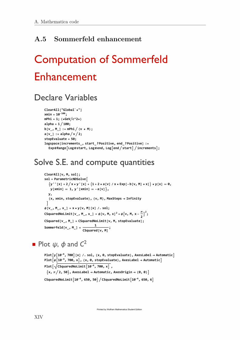
Computation of Sommerfeld
Enhancement
Declare VariablesClearAll["Global`*"]
xmin = 10-100;
mPhi = 1; (*GeVc^2*)
alpha = 1 100;
b[v_, M_] := mPhi (v * M);
a[v_] := alpha v 2;
stopEvaluate = 50;
logspace[increments_, start_?Positive, end_?Positive] :=
Exp@RangeLog@start, Log@end, Logend start increments;
Solve S.E. and compute quantitiesClearAll[v, M, sol];
sol = ParametricNDSolve
y''[x] + 2 x * y'[x] + 1 + 2 * a[v] / x * Exp[-b[v, M] * x] * y[x] ⩵ 0,
y[xmin] ⩵ 1, y'[xmin] ⩵ -a[v],
y,
x, xmin, stopEvaluate, v, M, MaxSteps → Infinity
ϕ[v_, M_, x_] = x * y[v, M][x] /. sol;
CSquaredNoLimit[v_, M_, x_] = ϕ[v, M, x]2+ ϕv, M, x -
π
22;
CSquared[v_, M_] = CSquaredNoLimit[v, M, stopEvaluate];
Sommerfeld[v_, M_] =1
CSquared[v, M];
◼ Plot ψ, ϕ and C2 Ploty10-4, 700[x] /. sol, x, 0, stopEvaluate, AxesLabel → Automatic
Plotϕ10-4, 700, x, x, 0, stopEvaluate, AxesLabel → Automatic
Plot CSquaredNoLimit10-4, 700, x ,
x, π 2, 50, AxesLabel → Automatic, AxesOrigin → 0, 0
CSquaredNoLimit10-4, 650, 50 CSquaredNoLimit10-4, 650, 6
Printed by Wolfram Mathematica Student Edition
A. Mathematica code
A.5 Sommerfeld enhancement
XIV
◼ Plot Sommerfeld for different massesLogLogPlot
Evaluate[
Table[
Sommerfeld[v, i],
i, 600, 650, 700, 750, 800
]
], v,1
910-5, 0.1,
PlotLegends → LineLegend600, 650, 700, 750, 800, LegendFunction →
Framed[#1, FrameMargins -> 0] & , LegendLabel → "DM Mass (GeV/c2)",
AxesLabel → "Velocity (c)", "Sommerfeld", ImageSize → 500,
Frame → True, FrameStyle → Directive[Black, 16],
FrameLabel → Style["Relative velocity [c]", 16], Style["S(v)", 16],
RotateLabel → False
◼ Plot Sommerfeld for different velocitiesLogPlot
Evaluate
Table
Sommerfeld10i, m,
i, -5, -2, 1
, m, 500, 900,
PlotLegends → LineLegend10-5 c, 10-4 c, 10-3 c, 10-2 c, LegendFunction →
Framed[#1, FrameMargins -> 0] & , LegendLabel → "Relative Velocity",
AxesLabel → "Velocity (c)", "Sommerfeld", AxesOrigin → 500, -10,
ImageSize → 500, Frame → True, FrameStyle → Directive[Black, 16],
FrameLabel → Style"Particle Mass [GeV/c2]", 16, Style["S(v)", 16],
RotateLabel → False
Check location of the resonance peak in DM Mass.
FindMaximumSommerfeld10-5, m, m, 700, 710
Refine data and construct tablevRange = logspace1000, 10-8, 0.1;
M = 750;
SommerfeldTable =
Table[v, Sommerfeld[v, M], v, vRange] // Timing;
SetDirectory[NotebookDirectory[]];
SommerfeldTable[[2]] >> "sommerfeldTable10_3_750";
SommerfeldTable[[1]]
3.23438
2 Sommerfeld_650_real (1).nb
Printed by Wolfram Mathematica Student Edition
SetDirectory[NotebookDirectory[]];
SommerfeldValues = << "sommerfeldTable10_3_750";
vRange = logspace1000, 10-8, 0.1;
SommerfeldMass = Interpolation[SommerfeldValues];
TSommerfeldValues = Transpose[SommerfeldValues];
PlotLog10@SommerfeldMass10v, v, -8, -1
vPad = logspace10, 10-8, 0.9 * 10-6;
TSommerfeldValuesDropped =
Map[
Drop[
#,
Position[#, Max[#[[All, 2]]]][[1]][[1]]
] &,
TSommerfeldValues,
1
];
TSommerfeldValuesPadded =
Map[
PadLeft[
#,
1010,
Table[
Flatten[vPad, vRange][[i]], #[[1, 1, 2]],
#[[1, 2]]
,
i, 1, Length[Flatten@vPad, vRange]
]
] &,
TSommerfeldValuesDropped,
1
];
(*Generate the sommerfeld tabel giving the interpolated function*)
TSommerfeldValuesPadded >> "SommerfeldTableComplete_750"
SommerfeldFunction = Interpolation[SommerfeldValues, InterpolationOrder → 1]
PlotLog10@SommerfeldFunction10v, v, -8, -1
Sommerfeld_650_real (1).nb 3
Printed by Wolfram Mathematica Student Edition
(*Galaxy constants*)
αDM = 1;
βDM = 3;
γDM = 1;
(*Units constants*)
cmPerKpc = 3.08567758 * 10^21.;
kgPerSunmass = 1.989 * 10^30.;
JoulePerKg = 2.99792458 * 10^8^2.;
geVPerJoule = 6.24150913 * 10^9.;
geVPerSunmass = kgPerSunmass * JoulePerKg * geVPerJoule;
pi = 3.14159265;
particelMass = 600;
G = 4.2994 * 10-6;
Off[NIntegrate::slwcon];
Off[NIntegrate::ncvb];
Fori = 1, i ≤ Length[galaxyArray], i++,
ClearAll[distance, radiusFunction, r0ρ0, galaxy, radiusFunction, JNew, Jnew];
galaxy = galaxyArray1[[i]];
SetDirectory[NotebookDirectory[]];
SetDirectory["data"];
SetDirectory["params"];
distance =
Import[ToString@StringForm["params_``.dat", galaxy], "Table"][[2]][[1]];
radiusFunction[s_, cosθ_] = distance^2. + s^2. - 2. s distance cosθ ;
JNew[r0_, ρ0_] := Log10
geVPerSunmass^2. * cmPerKpc^-5.
* 2. pi *
1.
v0[r0, ρ0]*
NIntegrate
rhoDM[radiusFunction[s, x], r0, ρ0]2.*
gammav0[r0, ρ0], radiusFunction[s, x] r0,
s, 0., ∞, x, Cos[θMax], 1.,
Method → "GlobalAdaptive", "SymbolicProcessing" → 0,
"SingularityDepth" → 10000 000, "MaxErrorIncreases" → 3000, MaxRecursion → 20
;
SetDirectory[NotebookDirectory[]];
SetDirectory["Completed"];
SetDirectory["Data"];
SetDirectory["Minimasation"];
r0ρ0 = Map[Drop[#, -1] &, Get[ToString[galaxy] <> "_r0ρ0rStarL"][[All, 1]]];
Jnew = Apply[JNew, r0ρ0, 1];
Put[Jnew, ToString[galaxy] <> "_J_new"];
;
Printed by Wolfram Mathematica Student Edition
A. Mathematica code
A.6 Calculated Js interpolated function
XVII


![VLT/UVES ABUNDANCES IN FOUR NEARBY DWARF SPHEROIDAL ...ganymede.nmsu.edu/holtz/talks/potsdam03/papers/shetrone.pdf · stars in these dSph galaxies ([Fe/H] < 1) have halo-like s- and](https://img.pdfslide.us/doc/110x75/5f7c43046076296c320dcc82/vltuves-abundances-in-four-nearby-dwarf-spheroidal-stars-in-these-dsph-galaxies.jpg)