Particle-hole pairs and density-density correlations

in the Lieb-Liniger model

J. De Nardis1 and M. Panfil2

1Departement de Physique, Ecole Normale Superieure, PSL Research University,

CNRS,

24 rue Lhomond, 75005 Paris, France2Institute of Theoretical Physics, University of Warsaw,

ul. Pasteura 5, 02-093 Warsaw, Poland

E-mail: jacopo.de.nardis@ens.fr, milosz.panfil@fuw.edu.pl

Abstract. We review the recently introduced thermodynamic form factors for pairs

of particle-hole excitations on finite-entropy states in the Lieb-Liniger model. We focus

on the density operator and we show how the form factors can be used for analytic

computations of dynamical correlation functions. We derive a new representation

for the form factors and we discuss some aspects of their structure. We rigorously

show that in the small momentum limit (or equivalently, on hydrodynamic scales) a

single particle-hole excitation fully saturates the spectral sum and we also discuss the

contribution from two particle-hole pairs. Finally we show that thermodynamic form

factors can be also used to study the ground state correlations and to derive the edge

exponents.

arX

iv:1

712.

0658

1v5

[co

nd-m

at.q

uant

-gas

] 3

0 M

ay 2

018

2

1 Introduction 3

2 The Lieb-Liniger model 5

3 Entropy of states and thermodynamic form factors 8

3.1 Thermodynamic form factors . . . . . . . . . . . . . . . . . . . . . . . . 10

4 A new expression for the thermodynamic form factors 12

4.1 Generalized particle-hole thermodynamic functions . . . . . . . . . . . . 14

5 Small momentum limit and single particle-hole contribution 16

5.1 Single particle-hole contribution and generalized detailed balance relation 17

5.2 Single particle-hole contribution and Generalized Hydrodynamics . . . . 19

6 Two and more particle-hole contributions 20

6.1 Two particle-hole contribution in the small momentum limit . . . . . . . 22

7 Dressing of particle-hole excitations at zero temperature 23

7.1 Non-critical states: smooth filling functions . . . . . . . . . . . . . . . . . 25

7.2 Critical states: dressing threshold k∗ . . . . . . . . . . . . . . . . . . . . 25

8 Dynamical correlations of the ground state in the small momentum

limit 28

9 Numerical evaluations 31

10 Conclusions 31

A Role of the averaging state 37

B Derivations 39

B.1 Fredholm determinant . . . . . . . . . . . . . . . . . . . . . . . . . . . . 39

B.2 Function W (hi, λ) . . . . . . . . . . . . . . . . . . . . . . . . . . . . . . . 40

B.3 Dependence on constants in the prefactor . . . . . . . . . . . . . . . . . . 41

B.4 Derivation of formula (125) . . . . . . . . . . . . . . . . . . . . . . . . . 43

C On the numerical evaluation of the Fredholm determinant 45

3

1. Introduction

The study of correlation functions of integrable models have a long history. Indeed,

it seems natural to expect a knowledge of correlation functions from models which are

exactly solvable. The reality however is more complicated and the question of computing

correlation functions turns out to be quite involved. Nowadays exact solvability, or

quantum integrability usually refers to the Bethe Ansatz methods of finding eigenstates

and eigenenergies. Methods of Bethe Ansatz have been successfully applied to very

different physical systems, ranging from condensed matter systems [1] through the

AdS/CFT correspondence [2] to supersymetric gauge theories [3].

With correlation functions the situation is different. The building blocks of the

correlation functions, form factors or matrix elements of local operators, are difficult to

compute. They are known only for some models and for some operators. Examples are

the Lieb-Liniger gas [4–8] or the XXZ spin chain [9, 10]. However, even knowing the

form factors, to get a correlation function a spectral sum has to be performed which is

an even more difficult challenge. The origin of these difficulties is in the same time the

reason of interest in integrable models.

The models under consideration are strongly correlated, which among other things,

means that form factors of physical operators, like density or field operators, computed

between two arbitrary eigenstates are generally non-zero. Of course it might happen

that symmetry forces the form factor to be zero, but unless this is the case, generally

they are not zero. This has to be compared with weakly correlated theories, where form

factors between two arbitrary eigenstates are generally zero. This way of thinking of

correlated systems goes back to the notion of orthogonality catastrophe [11].

Therefore strong correlations in these theories show up in two ways. The form

factors are complicated, rather than simple functions of the eigenstates. And in

computing the correlation functions, when the spectral sum must be evaluated, one

has to sum over a huge number of eigenstates. Some methods were developed to tackle

these problems.

In the first approach, instead of studying the full correlation functions, certain

special features of them were extracted. For example the ground states of gapless 1D

quantum models exhibit critical properties: the space-time correlation functions decay

as power laws. A theory of 1 dimensional quantum liquids, the Luttinger theory, predicts

a general asymptotic structure of correlation functions [12, 13]. By carefully analysing

the excitations responsible for that structure, it was possible to derive the asymptotic of

the space-time correlation functions directly from the integrable models [14–17]. This

has an advantage over a universal approach of the Luttinger liquid theory, it allows to

go beyond the field theory predictions and also to fix non-universal, model dependent,

constants appearing in the expression for the correlation function. These constants can

also be fixed without computing the correlation function, but only by computing the

effects of the excitations which are responsible for the corresponding part of correlation

function [16,18,19].

4

The second approach, which goes under the name of ABACUS [20], is to compute

correlation functions with the help of a computer. This direct approach relies on

knowledge of exact eigenstates, eigenenergies and form factors at finite system size. The

role of the computer is to evaluate the spectral sum term by term. As it is impossible

to sum over the whole Hilbert space, the key behind the ABACUS is to organize the sum

such that the more important excitations are summed first. This approach turned out

to be very successful in providing both qualitative and quantitative predictions for the

correlation functions in various physical situations, examples being the ground state [21]

and thermal correlation in some range of temperatures [22].

Another way is the so-called quantum transfer matrix approach [23]. There the

correlation functions are given by a series over matrix elements of a time-dependent

quantum transfer matrix rather than the Hamiltonian. Recently this approach has

brought also new results for the dynamical correlation functions at finite temperature

in lattice integrable models [24].

Finally methods from integrable field theories were also successfully implemented

in the study of dynamical correlations in spin chains [25–27].

In the work [28] we started a new approach based on the thermodynamic Bethe

ansatz. Motivated by a computation of the thermodynamic limit of the ground state

form factors [19] we considered the thermodynamic limit of form factors for a generic (but

non-critical) state. By non-critical state we mean a state in which correlation functions

do not exhibit critical behavior, e.g. the decay of spatial correlations is exponential.

This excludes for example, the ground state of the Lieb-Liniger model. Focusing on

non-critical states allowed us to derive a general expression for the thermodynamic

limit of the form factors of the density operators.

The thermodynamic form factors, however simpler in usage that their finite-size

versions are still too complicated for analytical computation of the whole spectral sum.

However certain simplifications happen when we consider correlation functions at small

momentum. In [29] we found a simple expression for the low-momentum static structure

factor of the Lieb-Liniger model for a generic non-critical state. It turned out that

this expression works also for the ground state, where in principle our approach is

not valid. Moreover we show there that at low momentum only a single particle-hole

excitation is necessary in order to saturate the full spectral sum. This surprising result

is related to the so-called generalized hydrodynamics theory [30,31], where the dynamics

of any integrable system at large scale is given by the ballistic motion of single particle

excitations.

In this work we review our studies of the thermodynamic form factors of the density

operator, focusing on various aspects of them. After the introductory part, the article

is divided in few sections which, to certain extent can be read independently. In section

3 we properly define the thermodynamic form factors. In section 4 we present and

derive a new representation for the thermodynamic limit of the form factors of the

density operator. Section 5 focuses on the density-density correlation function in the

small momentum limit. We present a new derivation of the detailed balance relation

5

and confirm predictions of the generalized hydrodynamics. In section 6 we connect

the expansion of the correlation function in the number of particle-hole pairs with an

expansion in powers of momentum. In section 7 we show the main difference between

the form factors for critical and non-critical states and we describe in which situations

we can still use the non-critical form factors to study critical systems. Based on this

result, in section 8 we derive the edge singularities of the ground state dynamic structure

factor in the small momentum limit. In section 9 we show that correlation functions

in the small momentum limit computed with these new form factors agrees with the

results obtained from the ABACUS algorithm. In Appendix A we display some open

questions regarding the structure of the form factors. Some more technical or longer

computations are placed in Appendix B. Appendix C discusses numerical evaluation of

the form factors.

2. The Lieb-Liniger model

The Hamiltonian of the Lieb-Liniger model is [1, 32]

H =

ˆ L

0

dx

(−ψ†(x)

∂2

∂x2ψ(x) + c ψ†(x)ψ†(x)ψ(x)ψ(x)

), (1)

where L is the length of the system, which we assume to be large, and ψ(x) is the

canonical Bose field

[ψ(x), ψ†(y)] = δ(x− y). (2)

The Hamiltonian describes a system of bosons on a line and it is a paradigmatic example

of a system of interacting bosons on the continuum, also experimentally relevant for

cold atomic physics [33–39]. Notable importance in the past years have had also its

non-equilibrium properties [40–42], especially after a quantum quench [40,43–52].

We consider a finite but very long system of length L with periodic boundary

conditions. Eigenstate are parametrized by a set of N momenta or rapidities λj which

solve the Bethe ansatz equations (29). We focus on the repulsive regime c ≥ 0, where

the λj are all real parameters, in contrast to the attractive regime c < 0 where they can

form bound states [53–55]. In the thermodynamic limit N,L → ∞ we can introduce

a function ρ(λ) which specifies the density of particles with rapidity λ. The density of

particles ρ(λ) is related to the filling function ϑ(λ) through the total density density of

states ρt(λ)

ϑ(λ) =ρ(λ)

ρt(λ). (3)

The total density function obeys the following integral equation

ρt(λ) =1

2π+

ˆ ∞−∞

dλ′ϑ(λ′)

2πK(λ− λ′)ρt(λ′), (4)

6

where the kernel K(λ) depends on the interaction strength c and is given by

K(λ) =2c

c2 + λ2. (5)

For convenience we introduce also a hole density function

ρh(λ) = ρt(λ)(1− ϑ(λ)). (6)

Let |ϑ〉 denotes a macroscopic eigenstate of the Lieb-Liniger Hamiltonian (whose

definition will be more extensively explained in section 3) in the thermodynamic limit

characterized by a filling function ϑ(λ) taking values in [0, 1]. The particle density,

momentum and energy are the consecutive moments of the density ρ(λ)

n ≡ N

L=

ˆ ∞−∞

dλ ρ(λ), (7)

P

L=

ˆ ∞−∞

dλλρ(λ), (8)

E

L=

ˆ ∞−∞

dλλ2ρ(λ). (9)

In the following we set the total density to unit value n = 1. We give few examples of

the filling function for physically interesting states. The filling function of the ground

state corresponds to a Fermi sea

ϑ(λ) =

{1, −q ≥ λ ≥ q,

0, otherwise,(10)

where q plays a role of the Fermi momentum. The ground state is an archetypical, and

the most important, critical state. Other interesting example of a critical state is the

split Fermi sea state introduced in [56]. The filling function for the finite temperature

state [57] is

ϑ(λ) =1

1 + exp(β(ε(λ)− µ)), (11)

where ε(λ) is the dressed energy (17) and µ the chemical potential. Other distributions

of interest are the generalized Gibbs ensemble (GGE) states [58–61], which are nothing

else than generalization of the thermal state (11), with β → β(λ) with β(λ) a positive

function [62,63]

ϑ(λ) =1

1 + exp(β(λ)(ε(λ)− µ)). (12)

Contrary to the ground state, the filling function for finite temperature and GGE states

is a smooth function of λ for any β(λ) <∞. We remark that since the total density of

the gas have to be finite, the functions ε(λ) and β(λ) must be such that´dλϑ(λ) <∞.

7

The excited states around |ϑ〉 are created by making a number of particle-hole

pairs in the filling function. An m particle-hole excited state we denote |ϑ; p,h〉, where

p = {pj}mj=1 and h = {hj}mj=1. Sets p and h specify the particle-hole content of the

excited state. The particle density for such an excited state is

ρ(λ; p,h) = ρ(λ) +1

L

m∑j=1

(δ(λ− pj)− δ(λ− hj))−1

L∂λρ(λ)

(F (λ|p,h)

ρt(λ)

)+O(L−2),

(13)

where the backflow function F (λ|p,h) =∑m

j=1 (F (λ|pj)− F (λ|hj)) is defined below.

There are also more general excited states with different number of particles and holes

but the form factors of the density operators vanishes for such states. An excited state

has relative (with respect to |ϑ〉) energy and momentum given by

k(ϑ; p,h) =m∑j=1

k(pj)− k(hj), (14)

ε(ϑ; p,h) =m∑j=1

ε(pj)− ε(hj). (15)

Functions k(λ) and ε(λ) are the dressed momentum and energy and are given by

k(λ) = λ+

ˆ ∞−∞

dαF (α|λ)ϑ(α), (16)

ε(λ) = λ2 +

ˆ ∞−∞

dαF (α|λ)ϑ(α)(2α). (17)

Here F (α|λ) is the backflow or shift function obeying

2πF (λ|α)=θ(λ− α) +

ˆ ∞−∞

dλ′ϑ(λ′)F (λ′|α)K(λ− λ′), (18)

where

θ(λ) = 2 arctan

(λ

c

). (19)

Notice that the total density of states ρt(λ) is the derivative of the dressed momentum

k′(λ) = 2πρt(λ). (20)

In this work we are concerned with the density-density correlation functions, also

known as a dynamic structure factor, DSF, in the thermodynamic limit at fixed total

density n. The density operator is

ρ(x) = ψ†(x)ψ(x), (21)

8

and its time evolution in the Heisenberg picture is given by the Lieb-Liniger Hamiltonian

ρ(x, t) = eiHtρ(x)e−iHt. (22)

The dynamical density-density correlation function of the state |ϑ〉 in the

thermodynamic limit is defined as

Sρ(x, t) = 〈ϑ|ρ(x, t)ρ(0, 0)|ϑ〉. (23)

Its Fourier transform, the dynamic structure factor, is given by

Sρ(k, ω) =

ˆ ∞−∞

dx

ˆ ∞−∞

dt ei(kx−ωt)S(x, t). (24)

In the spectral representation this can be written as a sum over a generic number of

pairs of particle-hole excitations on the reference state |ϑ〉 [28]

Sρ(k, ω) =∑m≥1

Smphρ (k, ω), (25)

where the contribution from m particle-hole pairs is given by

Smphρ (k, ω) =

(2π)2

(m!)2

∞−∞

dpmdhm|〈ϑ|ρ(0)|ϑ,h→ p〉|2δ(k − k(p,h))δ(ω − ω(p,h)).

(26)

Here the integration measure is defined as

dpmdhm =m∏j=1

dpjdhj ρ(hj)ρh(pj), (27)

and the finite part integral is defined as

∞−∞

dhf(h) = limε→0+

ˆ ∞+iε

−∞+iε

dh f(h) + πiresh=p

f(h). (28)

The finite part integral appears because the thermodynamic form factors |〈ϑ|ρ(0)|ϑ,h→p〉| have a single pole when pj coincides with hk, known as kinematic poles. In the next

section we review how to properly define the thermodynamic form factors on a generic

non-critical thermodynamic eigenstate |ϑ〉.

3. Entropy of states and thermodynamic form factors

In this section we review the definition of the thermodynamic form factors and formula

for the form factor of the density operator orginally presented in [28]. In order to define

the thermodynamic form factors 〈ϑ|ρ(0)|ϑ; h→ p〉 we proceed in the following way. We

consider a finite system with periodic boundary conditions. Then the eigenstates of the

Hamiltonian are parametrized by a set of quantum numbers {Ij}Nj=1, where N is the

9

number of particles. Physical quantities are expressed in terms of the rapidities which

are related to quantum numbers through Bethe equations

λj =2π

LIj +

N∑k 6=j=1

θ(λj − λk), j = 1, . . . , N. (29)

In the thermodynamic limit N,L→∞ with N/L = n fixed, the rapidities are described

through their density function, the particle density ρ(λ) which can be formally defined as

ρ(λ) = limN,L→∞

1

L

N∑j=1

δ(λ− λj). (30)

The particle density can be used to compute the filling function ϑ(λ) which then specifies

a thermodynamic state |ϑ〉. Let {Ij}Nj=1 be a set of quantum numbers specifying a Bethe

state such that in the thermodynamic limit its filling function is given by ϑ(λ). There

are many choices of quantum numbers leading to the same filling function, thus to the

same thermodynamic state |ϑ〉. Their number is expS[ϑ] where S[ϑ] is the extensive

Yang-Yang entropy [57]

S[ϑ] = L

ˆ ∞−∞

dλ (ρt(λ) log ρt(λ)− ρh(λ) log ρh(λ)− ρ(λ) log ρ(λ)) . (31)

We define the normalized thermodynamic state as

|ϑ〉 = limN,L→∞

exp

(−1

2S[ϑ]

)∑{Ij}

|{Ij}〉, (32)

where the summation is over all the eS[ϑ] microscopic states with the same ϑ(λ) in the

thermodynamic limit. Notice that this definition was introduced also in the context of

the Quench Action approach [64].

The density operator ρ(x), like all other local operators, acts almost diagonally,

which means that for a given excitation and a choice of {Ij} the set {Jj} is basically

fixed up to pairs of particle-hole excitations ph which correspond to changing the values

of some quantum numbers: ph ≡ {Ii → Ji}mi=1, for a number m small compared to the

system size L. This implies that the only non-zero matrix elements are the one where

right and left states are characterized by the same filling function in the thermodynamic

limit . The thermodynamic form factors then reads

〈ϑ|ρ(0)|ϑ,h→ p〉 = limL,N→∞

exp

(−1

2(S[ϑ] + S[ϑ, ph])

)Lm∑{Ij}

〈{Ij}|ρ(0)|{Ij + ph}〉,

(33)

where S[ϑ, ph] = S[ϑ] + O(L0) is the entropy of the right state. In order to take the

thermodynamic limit we choose a ph such that in the thermodynamic limit there is a

set of finite particle-hole pairs h → p in the space of rapidities λ. For each hole h and

10

particle p there are ∼ L possibilities for ph, which is the reason why we multiply times

Lm in (33). This degeneracy will be taken into account also by multiplying the square

of the thermodynamic form factors times the densities of state ρh(p)ρ(h). Notice that

this picture changes drastically when the quantum numbers {I0j } describe the ground

state or a state with a finite discontinuity in ϑ(λ) in the thermodynamic limit. In this

case the finite size form factors decay with a non-integer power of L [16, 19].

In our computations we assumed that each element of the sum is essentially the

same (for large system size) and therefore∑{Ij}

〈{Ij}|ρ(0)|{Ij + ph}〉 = exp (S[ϑ]) 〈{I0j }|ρ(0)|{I0j + ph}, (34)

where {I0j } is any of the states. Finally using (32) we obtain the definition of the

thermodynamic form factors

〈ϑ|ρ(0)|ϑ,h→ p〉 = exp

(1

2δS[ϑ,p,h]

)lim

L,N→∞Lm〈{I0j }|ρ(0)|{I0j + ph}〉. (35)

The differential entropy is defined as, see eq. (41),

δS[ϑ,p,h] = S[ϑ,p,h]− S[ϑ]. (36)

The state |{I0j }〉 is called the averaging state and can be any state with ϑ(λ) in the

thermodynamic limit. Computations of the thermodynamic limit of the form factors

simplify after a convenient choice of the averaging state. In our work [28] we have chosen

a uniform averaging state, meaning that for each interval [λ, λ + dλ] there are ρ(λ)dλ

uniformly distributed rapidities. The role of the averaging state and consequences of

different choices on the computation of thermodynamic limit of the form factors are

discussed in the appendix A.

3.1. Thermodynamic form factors

We recall here the formula for the form factors of the density operator ρ(x) acting in

position x = 0 in the thermodynamic limit. This formula was derived in [28] and after

a small change of notation that we describe later reads

|〈ϑ|ρ(0)|ϑ,h→ p〉| = A(ϑ,p,h)D(ϑ,p,h) exp (B(ϑ,p,h)) , (37)

where‡

A(ϑ,p,h) =m∏k=1

[F (hk)

(ρt(pk)ρt(hk))1/2

πF (pk)

sin πF (pk)

sin πF (hk)

πF (hk)

]‡ In the formula for the form factors presented in [28] and [29] there was a misprint and factor 1/2 in

front of the differential entropy δS[ϑ;p,h] was missing. Morevoer in [29] the last factor of B(ϑ, {pj , hj})was also missing. However, since both contributions scale like k, where k is the momentum of the excited

state, these factor do not contribute in the small momentum limit and do not change the results of

[29].

11

×m∏

i,j=1

[(pi − hj + ic)2

(hi,j + ic)(pi,j + ic)

]1/2 ∏mi<j=1 hi,jpi,j∏mi,j=1(pi − hj)

, (38)

B(ϑ,p,h) =− 1

4

ˆ +∞

−∞dλdλ′

(F (λ)− F (λ′)

λ− λ′

)2

− 1

2

ˆ +∞

−∞dλdλ′

(F (λ)F (λ′)

(λ− λ′ + ic)2

)

+m∑k=1

P

ˆ +∞

−∞dλ

F (λ)(hk − pk)(λ− hk)(λ− pk)

+

ˆ +∞

−∞dλ

F (λ)(pk − hk)(λ− hk + ic)(λ− pk + ic)

+1

2δS[ϑ; p,h] +

1

2

ˆdλϑ(λ)F ′(λ)πF (λ) cot(πF (λ)), (39)

D(ϑ,p,h) =c

2detmi,j=1 (δij +Wij)

Det(1− A)

Det(1− Kϑ). (40)

We now explain the main ingredients of this formula. The function ϑ(λ) is the filling

function characterizing a state and {p, h}mj=1 describe particle-hole excitations over this

state. F (λ) = F (λ|p,h) is the back-flow function (18). To shorten the formula we also

use a rescaled back-flow F (λ) = ϑ(λ)F (λ). Function δS[ϑ; p,h] is a differential entropy

defined as

δS[ϑ; p,h] =

ˆ ∞−∞

dλ s[ϑ;λ]∂

∂λ

(F (λ|p,h)

ρt(λ)

), (41)

where s[ϑ;λ] is the entropy density [57] expressible through the density functions (see

eq. (31))

s[ϑ;λ] = ρt(λ) log ρt(λ)− ρ(λ) log ρp(λ)− ρh(λ) log ρh(λ). (42)

The first determinant of D(ϑ,p,h) is of a square matrix with the same size as the

number of particle-hole pairs. Its matrix elements W (hi, hj) are defined as solutions to

the following linear integral equation

W (hi, λ)− P

ˆ ∞−∞

dαW (hi, α)a(α)

(K(α− λ)− 2

c

)= bi

(K(hi − λ)− 2

c

), (43)

with the vector bi given by

bi = −a[p,h]res(hi)

ϑ(hi)F (hi), (44)

where a[p,h](λ) is a function defined below and a[p,h]res(hi)

is its residue at λ = hi

a[p,h]res(hi)

= limλ→hi

(λ− hi)a[p,h](λ). (45)

The two other determinants of D(ϑ,p,h) are Fredholm determinants. The kernel A is

A(λ, λ′) = a[p,h](λ)

(K(λ− λ′)− 2

c

), (46)

12

where

a[p,h](λ) =sin[πϑ(λ)F (λ)]

2π sin[πF (λ)]

m∏k=1

(pk − λhk − λ

√K(pk − λ)

K(hk − λ)

)e−

c2P´∞−∞ dλ′ ϑ(λ

′)F (λ′)K(λ′−λ)λ′−λ .

The operator 1 represents the identity 1(λ, λ′) = δ(λ− λ′) and

Kϑ(λ, λ′) = K(λ− λ′)ϑ(λ′)

2π. (47)

Comparing with expressions presented in [28,29] in the present formula we changed the

sign of a[p,h](λ) which leads to: a minus sign in the Fredholm determinant Det(1− A),

a changes of sign in the integral equation (43) specifiying matrix elements W (hi, hj),

and a change of sign in expression (44) for bi. This last change is cancelled, because

computation of the residue (45) gives an extra minus sign.

In the expression for the form factors principal value integrals appear. We define

them as

P

ˆ b

a

dλf(λ)

λ− c= lim

ε→0

(ˆ c−ε

a

dλf(λ)

λ− c+

ˆ b

c+ε

dλf(λ)

λ− c

), a < c < b. (48)

In this notation

P

ˆ a

−a

dλ

λ= 0. (49)

The principal value integrals appear because of the need to regularize the

thermodynamic limit of certain terms in the form factors. In appendix A we recall how

the form of the principal value integral is connected with the choice of the averaging

state.

4. A new expression for the thermodynamic form factors

We will show now that the last part of the form factors can be written in a simpler form

D(ϑ,p,h) =detmi,j=1 (Aij +Bij)

Det(1 + L[p,h])Det(1− Kϑ

) . (50)

which is given only in terms of the “generalized particle-hole resolvent” L[p,h], see eq.

(59). This new expression is also simpler from the numerical evaluation point of view,

as only one extra solution of integral equation is needed in order to determine the full

form factor. Moreover we will see later that it leads to a much simpler expression of the

single particle-hole form factor (79) and of its small momentum limit. In this section

we will present the main idea behind the derivation of this new expression. Few more

technical steps are relegated to the appendix B. The matrix elements Aij, Bij, such

13

���������������

������

�������

���������������������������

�

�

�

�

�

�

�

�

�

�

���������

����

�

�

�

�

�

�

�

�

�

�

�������������

������������

�����

����

�����

��������������������

�����

�

�

�

�

�

�

�

�

�

�

�

�

�

�

�

�������

��

�

�

�

�

�

�

�

�

�

�

�

�

�

�

�

�

���������

�

-��� -��� ��� ����

���

���

���

���

���������������������������������������������������������������������������

�����������������������������������������������������������������������������������������������������������������������������������������������

���������������������������������������������������������������������������������������������������������������������������������������

���������������������

���������������������������������������������������������������������������������������

���������������������������������������������������������������������������������������������������������������������������������������������

�

� � ��

���

���

���

���

���

���������������������������������������������

�����������

�

�

�

�

�

�

�

�

�

�

��������

����

�

�

�

�

�

�

�

�

�

�

�������������

�����������������������������������������

�����

������

�

�

�

�

�

�

�

�

�

�

�

�

�

�

������

���

�

�

�

�

�

�

�

�

�

�

�

�

�

�

�����������

�

-��� -��� ��� ����

���

���

���

���

����������������������������������������������������������������������������������������������������������������������������������������������������������������������������������������������������������������������

���������������������������������������������������������������������������������������������������������������������������������������������������������������������

���������������������������������������������������������������������������

���������������������������������������������������������������������������������������������������������������������������������������������������

�

� � ��

���

���

���

���

���

���

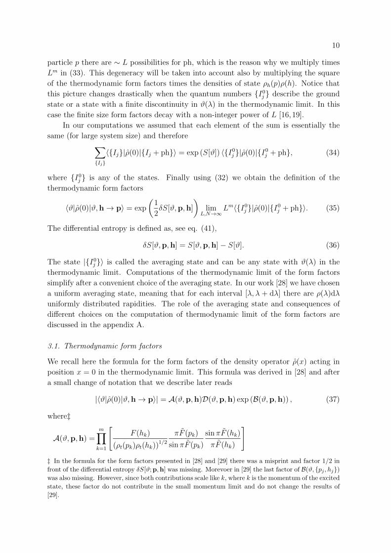
Figure 1. Dynamical structure factor (DSF) Sρ(k, ω) smoothed in energy ω by

convolving it with a Gaussian distribution of unit variance and evaluated at c = 4,

on thermal states with two different inverse temperatures β = 1 and β = 2 and

unitary density n = 1. Red data are obtained numerically by the ABACUS algorithm

while black continuous data are obtained by evaluations of the single particle-hole DSF

S1phρ (k, ω) (83). At k/kF = 0.2 (with kF = πn and ωF = k2F ) the single particle-hole

contribution completely saturates the full dynamical sum and Sρ(k, ω) ' S1phρ (k, ω),

while at large k = kF the two and higher particle-hole contributions are necessary in

order to compute the full DSF. For more details see section 9.

that Aij + Bij = δij + W (hi, hj), can be written in terms of “generalized particle-hole

thermodynamic functions”

Aij = δij −a[p,h]res(hi)

ϑ(hi)F (hi)

[limλ→hj

L[p,h](hi, λ)

a[p,h](λ)

], (51)

Bij =a[p,h]res(hi)

ϑ(hi)F (hi)2πρ

[p,h]t (hi)2πρ

[p,h]t (hj). (52)

14

which we will soon define. Notice that we have

detmi,j=1 (Aij) = 0, (53)

as we expect from the finite size expression of the form factors, see Appendix B.3. In the

course of the computation we will refer to the small momentum limit of the form factors

which we studied in [29]. By small momentum limit we mean computing form factors

between two states |ϑ〉 and |ϑ;h→ p〉 such that the momentum k (14) between the two

states is small. In section 5 we give more details on the small momentum limit. For

now we recall that in that case it was useful to introduce the resolvent of the kernel Kϑ

(1 + Lϑ)(1− Kϑ

)= 1 =

(1− Kϑ

)(1 + Lϑ), (54)

which obeys the following integral equation

Lϑ(λ, λ′) =ϑ(λ′)

2π

(K(λ− λ′) +

ˆ ∞−∞

dαLϑ(λ, α)K(α− λ′)). (55)

The resolvent is proportional to the derivative of the shift function (18), namely

Lϑ(µ, λ) = −ϑ(λ)∂µF (λ|µ). (56)

The introduction of the resolvent Lϑ allows for a number of simplifications which

lead to a simple expression for a form factors in the small momentum limit. Here

we generalize the approach of [29] to any momentum k, using a generalization of the

resolvent Lϑ(λ, λ′). The new generalized particle-hole thermodynamic functions reduce

to the standard ones in the small momentum limit, i.e. when the position of each particle

excitation coincides with the one of its hole.

4.1. Generalized particle-hole thermodynamic functions

We define a new kernel

K [p,h](λ, λ′) = K(λ, λ′)a[p,h](λ′). (57)

The resolvent of the new kernel is defined through(1 + L[p,h]

) (1−K [p,h]

)= 1 =

(1−K [p,h]

) (1 + L[p,h]

). (58)

We can write an integral equation for this generalized resolvent

L[p,h](λ, λ′) = a[p,h](λ′)

(K(λ− λ′) + P

ˆ ∞−∞

dαL[p,h](λ, α)K(α, λ′)

). (59)

Function a[p,h](λ) has simple poles whenever λ coincides with a position of a hole.

Iterating the equation we see that the poles of a[p,h](λ′) give rise to the poles of

15

L[p,h](λ, λ′). Consequently the particle-hole resolvent has simple poles for λ′ equal to

positions of holes. We can write an integral equation for the ratio L[p,h](λ, λ′)/a[p,h](λ′)

L[p,h](λ, λ′)

a[p,h](λ′)= K(λ− λ′) + P

ˆ ∞−∞

dα a[p,h](α)L[p,h](λ, α)

a[p,h](α)K(α, λ′). (60)

This form is convenient to study the small momentum limit of the single particle-hole

contribution. Under the principal value integral the poles of a[p,h](α) do not matter

and we can safely take the small momentum limit of a[p,h](α) which is ϑ(α)/(2π). In

turn the integral equation becomes an integral equation for the ratio 2πLϑ(λ, λ′)/ϑ(λ′),

c.f (55). Therefore

L[p,h](λ, λ′)

a[p,h](λ′)

p→h−−→ 2πLϑ(λ, λ′)

ϑ(λ′). (61)

We also define a generalization§ of the total density of rapidities ρ[p,h]t (λ) which is given

in terms of the resolvent L[p,h] as

2πρ[p,h]t (λ) = 1 + P

ˆ ∞−∞

dαL[p,h](λ, α). (62)

All these expression depends on the excitations through the a[p,h](λ) function. For a

single particle-hole pair in the small momentum limit p → h the generalized functions

reduce to the standard ones

a[p,h]p→h−−→ ϑ

2π, (63)

a[p,h]res(h)

p→h−−→ (p− h)ϑ(h)

2π, (64)

K [p,h] p→h−−→ Kϑ, (65)

L[p,h] p→h−−→ Lϑ, (66)

ρ[p,h]t

p→h−−→ ρt. (67)

We follow now the same strategy as in the small momentum limit and rewrite the

Fredholm determinant Det(1 − A) and solve for function W (λ, λ′). The computations

are presented in appendix B. For the Fredholm determinant we find

Det

(1− a[p,h]

(K − 2

c

))=

(1 +

2n[p,h]

c

)Det

(1−K [p,h]

), (68)

where n[p,h] is a generalization of the density of the gas‖

n[p,h] = P

ˆ ∞−∞

dλρ[p,h]t (λ)(2πa[p,h](λ)), n[p,h] p→h−−→ n. (69)

§ We mean here that ρ[p,h]t (λ) obeys a similar integral equation to the one obeyed by ρt(λ) and in

the small momentum limit is equal to ρt(λ). However we do not attempt here to give a physical

interpretation of the relation beween ρ[p,h]t (λ) and the total density of states ρt(λ).

‖ The remark of footnote 3 applies also here.

16

For the matrix elements Aij, Bij we find the result of equation (51), which, in the small

momentum limit and for single particle-hole excitation, gives

A11 = 0 (70)

B11p→h−−→ 2πρt(h)ρ(h)

Lϑ(h, h), (71)

in agreement with the results of [29].

5. Small momentum limit and single particle-hole contribution

We review here the results found in [29] for the small momentum limit of the dynamical

correlation functions and the single particle-hole contribution. Despite this is a well

studied limit, see for example [65–67] very few results are available in this limit

for thermal and non-thermal correlations. In [29] we considered a single particle-

hole excitation in the limit of small total momentum k = k(p) − k(h) and energy

ω = ε(p)− ε(h). By small momentum we mean that k is small compared with another

scale set by the interaction parameter c. Therefore for large values of c the small

momentum limit is actually a valid approximation over a large range of momenta. The

shift function is related to the resolvent Lϑ by

F (λ|p, h) = − 1

ϑ(λ)

ˆ p

h

dα Lϑ(α, λ), (72)

which in the small momentum limit leads to

F (λ) = −k Lϑ(h, λ)

ϑ(λ)+O(k2). (73)

The position of the particle and the hole can be expressed as functions of momentum

and energy by solving the following equations

p = h+k

k′(h)+O(k2), (74)

ω

k= v

(h+

k

2k′(h)

)+O(k2), (75)

with the dressed group velocity v(λ) associated to the rapidity λ defined by

v(λ) =dε(λ)

dk(λ). (76)

Given momentum k and energy ω, eq. (75) is solved for the hole position h. Then

position of particle p is found from (74). The DSF at small momentum is given by by

the single particle-hole contribution. Namely the single particle-hole contribution to the

DSF fully gives the DSF up to (positive) corrections of order k, see Fig. 1 and section 6

Sρ(k, ω) = S1phρ (k, ω) (1 +O(k)) . (77)

17

The single particle-hole contribution in the small momentum limit is given by

S1phρ (k, ω) ' (2π)2

ρ(h)ρh(p)

|kv′(h)k′(h)|

∣∣∣〈ϑ|ρ|ϑ, h→ p〉∣∣∣2, (78)

with h, p fixed by conditions (74) and (75). The full single particle-hole form factors is

given by

|〈ϑ|ρ(0)|ϑ, h→ p〉| = 2πρ[p,h]t (h)ρ

[p,h]t (h)√

ρt(p)ρt(h)

πF (p)

sin πF (p)

sin πF (h)

πF (h)

sin[πF (h)]

ϑ(h) sin[πF (h)]

× e−c2P´∞−∞ dλ′ ϑ(λ

′)F (λ′)K(λ′−h)λ′−h exp (B(ϑ, [p, h]))

Det(1−K [p,h]

)Det(1− Kϑ

) , (79)

and its limit p→ h is remarkably simple

|〈ϑ|ρ(0)|ϑ, h→ p〉| = k′(h) +O(p− h). (80)

Notice that the denominator |kv′(h)k′(h)| in S1phρ (k, ω) comes from the Jacobian of the

change of variable (p, h) → (ω, k) in the small k limit. Computing the static structure

factor one finds the compressibility ∂n∂µ

of the gas, which is the correct result for any

finite temperature state

limk→0

ˆ ∞−∞

Sρ(k, ω)dω

2π=∂n

∂µ, (81)

with µ the chemical potential. At zero temperature eq. (78) leads toˆ ∞−∞

Sρ(k, ω)dω

2π=|k|vs

+O(k2), (82)

with vs = v(q) and q the Fermi momentum k(q) = kF = πn.

5.1. Single particle-hole contribution and generalized detailed balance relation

We here review the derivation of the detailed balance relation valid at small momentum

k, as originally found in [29]. We consider the exact single particle-hole DSF

S1phρ (k, ω) =

(ϑ(h)(1− ϑ(p))

)|〈ϑ|ρ(0)|ϑ, h→ p〉|2 k

′(h)k′(p)

| det Jp,h|, (83)

with position of particle and hole fixed by ω = ε(p) − ε(h) and k = k(p) − k(h), with

the form factors given in (79) and the Jacobian of the change of variable (p, h)→ (ω, k)

Jp,h =

(ε′(p) ε′(h)

k′(p) k′(h)

). (84)

We consider the ratio between the response of the system at positive and negative

momenta and energiesSρ(−k,−ω)

Sρ(k, ω), (85)

18

which for thermal states is known to be equal to eβω. Since the excitation with particle-

hole (p, h) has energy ω = ε(p)−ε(h) and momentum k = k(p)−k(h), the excitation with

energy −ω and momentum −k is the one with particle-hole given by (h, p). Therefore

the ratio of the the single particle-hole DSF is given by

S1phρ (k, ω)

S1phρ (−k,−ω)

=ϑ(h) (1− ϑ(p))

ϑ(p) (1− ϑ(h))

|〈ϑ|ρ(0)|ϑ,h→p〉|2| det Jp,h|

|〈ϑ|ρ(0)|ϑ,p→h〉|2| det Jh,p|

. (86)

The symmetry of the Jacobian implies that |Jp,h| = |Jh,p|. Numerically we observe that

|〈ϑ|ρ(0)|ϑ, h→ p〉|2

|〈ϑ|ρ(0)|ϑ, p→ h〉|2= 1, (87)

which implies a particle-hole symmetry of the single particle-hole form factors. It would

be desiderable to prove it analytically from the expression (79), but we were not able to

do so. Consider now a thermal state: using ϑ(λ) = (1 + eβ(ε(λ)−µ))−1we have

ϑ(h) (1− ϑ(p))

ϑ(p) (1− ϑ(h))= eβ(ε(p)−ε(h)) = eβω. (88)

We now consider non-thermal, parity invariant states, namely such thatˆdλϑ(λ)λ2n+1 = 0, (89)

for any integer n. For such states with ϑ(λ) = (1 + e(β(λ)ε(λ)−µ))−1 we have

ϑ(h) (1− ϑ(p))

ϑ(p) (1− ϑ(h))= e(ε(p)β(p)−ε(h)β(h)). (90)

In the small momentum limit with p = h+ k/k′(h) this last equation can be expanded

in k and we obtain¶S1phρ (k, ω)

S1phρ (−k,−ω)

= eF(k,ω) +O(k2), (91)

where the function F(k, ω) depends only on the state |ϑ〉, analogously to the thermal

equilibrium case, and is given by

F(k, ω) = k∂ log(ϑ−1(h)− 1)

∂k(h)

∣∣∣h=v−1(ω/k)

, (92)

with the dressed velocity v(h) given in equation (76). While this relation is valid only for

the single particle-hole contribution, using the result of equation (108) we can show that

at order k, namely on Euler hydrodynamic scales, the DSF satisfies a detailed balance

relation for any parity invariant reference state |ϑ〉

Sρ(k, ω)

Sρ(−k,−ω)= eF(k,ω) +O(k2), (93)

¶ If the state is parity invariant, ϑ(λ) = ϑ(−λ), then the correlation function obeys exactly Sρ(k, ω) =

Sρ(−k, ω).

19

as originally found in [29]. This form of generalized detailed balance allowed in [63] to

effectively “measure” the distribution ϑ(λ) (and therefore its generalized temperatures

β(λ)) by a measurement of Sρ(k, ω). We expect the same form of detailed balance

relation for any operator that creates only pairs of particle-hole excitations, i.e. that

conserves the total number of particles.

For a thermal state instead detailed balance is exact at any value of momentum k,

S(k, ω) = eβωS(−k,−ω). Indeed, from equation (88) and (87) we obtain that for any k

and thermal states |ϑ〉S1phρ (k, ω)

S1phρ (−k,−ω)

= eβω. (94)

This implies that when |ϑ〉 is a thermal state each m-th particle-hole contribution

satisfies independently the detailed balance relation: Smphρ (k, ω) = Smph

ρ (−k,−ω)eβω.

5.2. Single particle-hole contribution and Generalized Hydrodynamics

We show here that what was found in [29], namely that the small momentum limit of

the density DSF is given by the single particle-hole contribution

limk,ω→0ωk=κ

Sρ(k, ω) = limk,ω→0ωk=κ

S1phρ (k, ω), (95)

and that its small momentum limit is given in terms of the inverse of the dressed velocity

v(h) (76)

limk,ω→0ωk=κ

S1phρ (k, ω) = (2π)2

ρ(h)ρh(h)

|kv′(h)k′(h)|(k′(h))

2∣∣∣h=v−1(κ)

, (96)

is compatible with the predictions of Generalized Hydrodynamics (GHD) [30,31]. In the

context of GHD it was shown [68,69] that given the density q(x) of a generic conserved

operator Q =´q(x)dx, such that [H, Q] = 0, the hydrodynamic description of the

excitations implies a generic form for the asymptotic correlations

〈q(x, t)q(0, 0)〉 ' (2π)

ˆdhδ(x− v(h)t)ρ(h)(1− ϑ(h))(qdr(h))2, (97)

at large x and t with x/t fixed (the so-called Euler scale) and with the dressed single-

particle eigenvalue of the charge given by

qdr(h) = q(h) +

ˆ ∞−∞

dαLϑ(h, α)q(α). (98)

with Lϑ(λ, µ) the resolvent (55) and q(λ) the eigenvalue of the charge Q on a single

particle state |λ〉. Going to Fourier space this result implies the following form for the

DSF at small momentum and energy

Sq(k, ω) ' (2π)

ˆdhδ(ω−v(h)k)ρ(h)(1−ϑ(h))(qdr(h))2 = (2π)

ρ(h)(1− ϑ(h))(qdr(h))2

|kv′(h)|,

(99)

20

which is in accord with our result for the density DSF (96) after using that

k′(h) = ndr = 2πρt(h) with n = 1. (100)

GHD therefore implies that the result (96) and (95) also applies to the DSF of any

globally conserved operator Sq(k, ω). Namely that in the small momentum limit this is

saturated by the single particle-hole contribution with amplitude given by

limk,ω→0ωk=κ

Sq(k, ω) = (2π)2ρ(h)ρh(h)

|kv′(h)k′(h)|

[limp→h

∣∣∣〈ϑ|q|ϑ, h→ p〉∣∣∣2]∣∣∣

h=v−1(κ), (101)

with the following universal form for the form factors in the small momentum limit

limp→h|〈ϑ|q|ϑ, h→ p〉| = qdr(h). (102)

However GHD does not provide the corrections O(p − h) and in general it only

incorporates the leading term (80), in the small momentum limit, of the full single

particle-hole form factor (79). Up to now the only method to get the full form factor

expression is by taking the thermodynamic limit of the finite size expressions as we do

here for the density operator ρ(x).

6. Two and more particle-hole contributions

In this section we analyze higher order (in number of particle-hole pairs) contributions

to the DSF. The analysis at small momentum shows that the DSF is organized in the

particle-hole contributions

Sρ(k, ω) =∑m≥1

Smphρ (k, ω), (103)

where each contribution at small k is of order

Smphρ (k, ω) ∼ O(km−2). (104)

We will show that this is the case first for the 2 particle-hole contribution. The

generalization to arbitrary number of particle-hole pairs will then follow immediately.

According to eq. (26) this contribution is given by

S2phρ (k, ω) =

1

4

ˆdh1 ρ(h1)

dp1ρh(p1)

ˆdh2 ρ(h2)

dp2ρh(p2)|〈ϑ|ρ(0)|ϑ,h→ p〉|2

× δ(ω − ε(p1)− ε(p2) + ε(h1) + ε(h2))δ(k − k(p1)− k(p2) + k(h1) + k(h2)).

(105)

We are not interested in precise evaluation of this formula, but just in establishing the

leading order k. To this end we change variables in the integrals, from h1, p1 to the

21

variables ε1 = ε(p1)− ε(h1), k1 = k(p1)− k(h1). We do the same for h2, p2 with ε2, k2.

We obtain

S2phρ (k, ω) =

1

4

dk1dk2

ˆdε1dε2 ρ(h1)ρh(p1) ρ(h2)ρh(p2)

|〈ϑ|ρ(0)|ϑ,h→ p〉|2

| det Jp1,h1 det Jp2,h2|δ(ω − ε1 − ε2)δ(k − k1 − k2), (106)

with position of holes and particles expressed in terms of εi, ki and the Jacobian as

in (84). The integrations of over k2 and ε2 can be performed what fix their values by

the momentum energy conservation

S2phρ (k, ω) =

1

4

dk1

ˆdε1 ρ(h1)ρh(p1) ρ(h2)ρh(p2)

|〈ϑ|ρ(0)|ϑ,h→ p〉|2

| det Jp1,h1 det Jp2,h2 |. (107)

We now restrict to the regime where k is small and ω/k is finite. In this limit k1 and

k2 = (k − k1) are both small. Therefore the particle-hole pairs corresponding to k1 and

k2 are also small. In the next subsection we show that the form factors in this limit

has a leading part of order k0. The integrals are both of order k (the energy is, in this

limit, a linear function of k) and the Jacobians are also of order k. Therefore (107) is of

order k0 and it gives a subleading term to the single particle-hole contribution S1phρ (k, ω)

which is of order k−1 +. Extending the logic to m particle-hole is straightforward. The

form factors, for arbitrary number of particle-hole excitations, is always of order k0.

Each integration over a pair of particle-hole can be converted into corresponding energy

and momentum conservations divided by the Jacobian. This bring a factor k for each

particle-hole pair and the momentum and energy conservation eliminate two of the

integrals, giving the final order km−2. The same logic is expected to be applicable

to the DSF of any particle-conserving operator q. Such an operator indeed can only

create particle-hole pairs and therefore the same arguments apply, provided that its

form factors are of order k0.

Notice that even if the leading two particle-hole contribution (107) is of order 1,

this does not spoil the detailed balance in the linear order in k, equation (91). This

is because S2phρ (k, ω) is an even function of ω for symmetric states (This is because, in

the leading order in k the 2 particle-hole form factors has a particle-hole symmetry.)

Therefore taking S1phρ (k, ω) = |k|S1ph

ρ (k, ω) ∼ O(k0) and expanding the ratio of the

DSF computed with opposite energies we obtain

Sρ(k, ω)

Sρ(k,−ω)=

S1phρ (k, ω) + |k|S2ph

ρ (k, ω)

S1phρ (−k,−ω) + |k|S2ph

ρ (k, ω)+O(k2)

=S1phρ (k, ω)

S1phρ (−k,−ω)

− |k|S2phρ (k, ω)

(S1phρ (k, ω)− S1ph

ρ (−k,−ω))(S1phρ (−k,−ω)

)2 +O(k2).

(108)

+ Notice that this implies that static structure factor also has a linear coefficient in k such as´S(k, ω)dω2π = S(0) + O(k) + O(k2). On the other hand usually, for small temperatures at least,

the terms proportional to k as such as the ones coming from (107) are small.

22

Since (S1phρ (k, ω) − S1ph

ρ (−k,−ω)) ∼ O(k) the second term is also of order k2, leading

to the detailed balance expression (91)

Sρ(k, ω)

Sρ(−k,−ω)=

S1phρ (k, ω)

S1phρ (−k,−ω)

+O(k2) = eF(k,ω) +O(k2). (109)

6.1. Two particle-hole contribution in the small momentum limit

We here show that in the small momentum limit, with p1 = h1 + k1/k′(h1) and

p2 = h2 + (1 − k1)/k′(h2) and k1 → kκ with k → 0, we have a well defined form

factor as function of h1, h2 and κ analogously to the single particle-hole case (80). For

such excitations the shift function is given simply by the sum of the shift function for

each excitation

F (λ) = − 1

ϑ(λ)

((p1 − h1)Lϑ(h1, λ) + (p2 − h2)Lϑ(h2, λ)

)+O(k2). (110)

In the form factors the only relevant piece is the matrices Aij and Bij, as almost all the

others are close to one (except few terms from A(ϑ,p,h)), as F (λ) ∼ k in the small

momentum limit. We have

a[p,h]res(hi)

p→h−−−→ −(p1 − hi)(p2 − hi)(hj − hi)j 6=i

ϑ(hi)

2π, i, j = 1, 2, (111)

and [limλ→hj

L[p,h](hi, λ)

a[p,h](λ)

]p→h−−−→ 2πLϑ(hi, hj)

ϑ(hj). (112)

Neglecting corrections of order k (namely we set p1−p2h1−h2 = 1 and p1−h2

h1−h2 = 1) we obtain

for the matrices Aij and Bij

Aij =

1− (p1−h1)Lϑ(h1,h1)(p1−h1)Lϑ(h1,h1)+(p2−h2)Lϑ(h2,h1)

−ϑ(h1)ϑ(h2)

(p1−h1)Lϑ(h1,h2)(p1−h1)Lϑ(h1,h1)+(p2−h2)Lϑ(h2,h1)

−ϑ(h2)ϑ(h1)

(p2−h2)Lϑ(h2,h1)(p1−h1)Lϑ(h1,h2)+(p2−h2)Lϑ(h2,h2)

1− (p2−h2)Lϑ(h2,h2)(p1−h1)Lϑ(h1,h2)+(p2−h2)Lϑ(h2,h2)

,

(113)

Bij =

((p1−h1)ρ(h1)(2π)ρt(h1)

(p1−h1)Lϑ(h1,h1)+(p2−h2)Lϑ(h2,h1)(p1−h1)ρ(h1)(2π)ρt(h2)

(p1−h1)Lϑ(h1,h1)+(p2−h2)Lϑ(h2,h1)(p2−h2)ρ(h2)(2π)ρt(h1)

(p1−h1)Lϑ(h1,h2)+(p2−h2)Lϑ(h2,h2)(p2−h2)ρ(h2)(2π)ρt(h2)

(p1−h1)Lϑ(h1,h2)+(p2−h2)Lϑ(h2,h2)

). (114)

The determinant of Aij is zero as it should, see (53) and Appendix B.3. The full form

factors in the leading order in k, which means the leading order in pj − hj, then reads

|〈ϑ|ρ(0)|ϑ, {h1, h2} → {p1, p2}〉| =2∏

k=1

F (hk)

ρt(hk)(pk − hk)det (Aij +Bij) +O(k1)

=( k1k′(h1)

2πρt(h1) +(1− k1)k′(h2)

2πρt(h2))

×

(Lϑ(h1, h2)

ρ(h2)

k′(h2)

1− k1+Lϑ(h2, h1)

ρ(h1)

k′(h1)

k1

)+O(k1). (115)

23

By rescaling k1 → κk and taking the limit k → 0 it is easy to see that the whole form

factor is of order k0. Increasing number of particle-hole pairs simply extends the product

and the matrices. The structure is however the same and form factors for any number

of particle-hole pairs in the small momentum limit is of order k0. Notice that for large

values of the coupling c, the resolvent vanishes as Lϑ(h1, h2) ∼ 1/c and therefore the

two-particle hole contribution S2phρ decays as 1/c2 as expected.

7. Dressing of particle-hole excitations at zero temperature

In this section we study the behavior of the form factors when the thermodynamic state

|ϑ〉 represents a critical state. The discontinuities in the filling function ϑ(λ) affect the

structure of the thermodynamic form factors and excitations created in the vicinity of the

discontinuities lead to divergences. A priori this is not a surprise. The thermodynamic

limit of the form factors was derived in [28] under an assumption that the filling function

is smooth and therefore using it to study correlation functions of critical states seems

problematic. However, in [29] we have shown that computing the small momentum limit

of the ground state static structure factor leads to a correct answer. In this section we

show that in general we can extract small momentum information about the critical

states from the form factors.

To show the difference between the critical and non-critical states we will consider

form factors with an excited state consisting of one dominant excitation, carrying most

of the momentum and energy of the excited state, and many small excitations, namely

with vanishing energy and momentum, that dress it (soft modes). In the two following

sections we consider what happens when the state is non-critical (smooth filling function)

and when the state is critical (discontinuous filling function). In the first case the

contribution from these form factors has zero measure and no dressing is needed for each

particle-hole excitation. In the second case, the form factors can be divergent when the

soft modes are localized in the vicinity of the discontinuities of the filling function, i.e.

the Fermi momenta. We show that this implies that for a single particle-hole excitation

with momentum k ≥ k∗ its form factors must be dressed with soft modes excitations

whose contribution is not negligible. We denote this as the dressing threshold k∗

k∗ =∣∣∣ √

K

2∂qF (q, q)

∣∣∣, (116)

with q the Fermi momentum and K the Luttinger liquid parameter 2πρt(q) =√K. In

the next session 8 will also show that in the small momentum limit the DSF close to the

two edges (in correspondence with the Lieb I and II dispersion relations ε1(k), ε2(k)) we

have

S(k, ω) ∼∣∣∣ω − ε1,2(k)

∣∣∣∓k/k∗ . (117)

Therefore when k ≥ k∗ the DSF S(k, ω) displays a non-integrable singularity at ω = ε1,

which signals a divergence of the contributions given by the soft modes to the form

factors.

24

We consider one single dominant particle-hole excitation and m soft modes. Recall

that each particle-hole excitation contributes k(pi, hi) = k(pi) − k(hi) and ε(pi, hi) =

ε(pi)−ε(hi) to the momentum and the energy. We assume that {p0, h0} pair is dominant,

that isk − k(p0, h0)

k� 1,

ω − ε(p0, h0)ω

� 1. (118)

In other words, for finite k and ω we have

1

k

m∑i=1

k(pi, hi)� 1,1

ω

m∑i=1

ε(pi, hi)� 1. (119)

The momentum and energy of the particle hole pair are, c.f. eqs. (14) and (15),

k(pi, hi) = pi − hi −ˆ ∞−∞

dλϑ(λ)F (λ|pi, hi), (120)

ε(pi, hi) = p2i − h2i − 2

ˆ ∞−∞

dλλϑ(λ)F (λ|pi, hi). (121)

For the left hand side to be small, the difference pi − hi must be small. Then the

back-flow simplifies

F (λ|pi, hi) = −(pi − hi)Lϑ(hi, λ)

ϑ(λ)+O((pi − hi)2). (122)

For the ground state these small excitations are only possible in the vicinity of the

Fermi edges ±q. For a generic state the small excitations can be created along the

whole distribution of rapidities. The total back flow is

F (λ|{pi, hi}) = F (λ|p0, h0)−m∑i=1

(pi − hi)Lϑ(hi, λ)

ϑ(λ), (123)

and is dominated by the back-flow of the dominating excitation. Let us write

F0(λ) = F (λ|p0, h0). (124)

We compute now the leading part of the form-factor in the particle-hole difference

pi − hi of the small excitations. The result is

|〈ϑ|ρ(0)|ϑ, {hj → pj}mj=0〉| = |〈ϑ|ρ(0)|ϑ, {ho → po}〉|

[m∏k=1

F0(hk)

ρt(hk)

ϑ(pk) sinπϑ(hk)F0(hk)

ϑ(hk) sinπϑ(pk)F0(pk)

]

×∏m

i<j=1(hi − hj)(pi − pj)∏mi,j=1(pi − hj)

exp

(m∑k=1

P

ˆ +∞

−∞dλ

F (λ)(hk − pk)(λ− hk)(λ− pk)

), (125)

and its derivation is given in Appendix B.4.

25

7.1. Non-critical states: smooth filling functions

We analyze now the contribution of the form-factors with a single dominant excitation

to the correlation function of a non-critical state. The filling function is smooth and

from eq. (125) we get

|〈ϑ|ρ(0)|ϑ,p,h〉| = |〈ϑ|ρ(0)|ϑ, p0, h0〉|

[m∏k=1

F0(hk)

ρt(hk)

] ∏mi<j=1(hi − hj)(pi − pj)∏m

i,j=1(pi − hj). (126)

Consider the (m+ 1) particle hole contribution to the correlation function

Am =

dpm+1dhm+1|〈ϑ|ρ(0)|ϑ,p,h〉|2δ(k − k(p,h))δ(ω − ε(p,h)), (127)

where we use the finite part integral. Restricting the integral over the m particle-hole

pairs to small excitations we obtain

Am =

dp0dh0|〈ϑ|ρ(0)|ϑ,p,h〉|2Bm(k, ω, p0, h0)δ(k − k0)δ(ω − ω0), (128)

where

Bm =

dpmdhm

[m∏k=1

F0(hk)

ρt(hk)

∏mi<j=1(hi − hj)(pi − pj)∏m

i,j=1(pi − hj)

]2. (129)

The integral in Bm is over regions where pi−hi is small so that the approximation to the

form factors can be used. We also used that the momentum and energy is determined

mainly by the dominant excitation to simplify the Dirac’s δ-function. The corrections

are proportional to (pi−hi) and can be neglected. The integrand in Bm has a double pole

whenever positions of particle and hole coincide. These double poles are regularized by

the finite part integral according to the prescription (28). Therefore Bm is finite. Each

finite part integral is over a small region of holes around the position of particles. This

is the phase space given to soft modes and Bm is roughly proportional to the volume

of the phase space that we allow for them. This implies that if we consider a single

particle-hole excitation and we dress it with soft modes, their contribution vanishes in

the limit of a vanishing phase space. Therefore there is no dressing of the form factors

for non-critical states. The situation is different if the state is critical, as the form factors

has poles when the small particle-hole excitations are taken close to the edges of the

Fermi sea.

7.2. Critical states: dressing threshold k∗

Let us consider the archetypical critical state, the ground state. For the ground state the

filling function ϑ(λ) equals to 1 for λ ∈ [−q, q] and zero otherwise. Therefore particles

must have |pj| > q while holes |hj| < q. For the form factors we get

|〈ϑ|ρ(0)|ϑ,h→ p〉| = |〈ϑ|ρ(0)|ϑ, p0, h0〉|

[m∏k=1

sin πF (hk)

πρt(hk)

] ∏mi<j=1(hi − hj)(pi − pj)∏m

i,j=1(pi − hj)

26

× exp

(m∑k=1

P

ˆ ∞−∞

dλϑ(λ)F0(λ)(hk − pk)

(λ− hk)(λ− pk)

). (130)

Let us focus on a single excitation and analyse the structure of the principal value

integral. We seperate the particle and hole parts

(hk − pk)(λ− hk)(λ− pk)

=1

λ− hk− 1

λ− pk, (131)

and consider first the hole contribution. We have

P

ˆ ∞−∞

dλϑ(λ)F0(λ)

λ− hk= lim

ε→0

(ˆ hk−ε

−∞dλ

ϑ(λ)F0(λ)

λ− hk+

ˆ ∞hk+ε

dλϑ(λ)F0(λ)

λ− hk

)= lim

ε→0

(ˆ hk−ε

−qdλ

F0(λ)

λ− hk+

ˆ q

hk+ε

dλF0(λ)

λ− hk

), (132)

where in the first line we used the definition of the principal value integral and in the

second line we used that the filling function vanishes beyond the interval [−q, q] and is

1 within. For the excitation to be small, position of the hole must be close to one of the

edges. Let us assume that hk ∼ q. Then the second integral can be simplified, making

an error of order q − hk, in the following way

P

ˆ ∞−∞

dλϑ(λ)F0(λ)

λ− hk= lim

ε→0

(ˆ hk−ε

−qdλ

F0(λ)

λ− hk+ F0(q) log

q − hkε

)= lim

ε→0

(ˆ hk−ε

−qdλ

F0(λ)

λ− hk− F0(q) log ε

)+ F0(q) log(q − hk).

(133)

The first expression is smooth as a function of hk thus we can set hk = q. Therefore for

a hole in the vicinity of q we get

P

ˆ ∞−∞

dλϑ(λ)F0(λ)

λ− hk= P+

ˆ q

−qdλ

F0(λ)

λ− q+ F0(q) log(q − hk), (134)

where we defined a version of the principal value integral with the pole at the boundary

P+

ˆ b

a

dλf(λ)

λ− b= lim

ε→0

(ˆ b−ε

a

dλf(λ)

λ− b− f(b) log ε

). (135)

Similar situation happens for the particle part and we find

P

ˆ ∞−∞

dλϑ(λ)F0(λ)

λ− pk= P+

ˆ q

−qdλ

F0(λ)

λ− q+ F0(q) log(q − pk). (136)

The whole principal value integral becomes

P

ˆ ∞−∞

dλϑ(λ)F0(λ)(hk − pk)

(λ− hk)(λ− pk)= P+

ˆ q

−qdλ

F0(λ)(hk − pk)(λ− hk)(λ− pk)

+ F0(q) logq − hkq − pk

.

(137)

27

The contribution of the P+ integral is bounded and proportional to pk − hk. Therefore

it can be neglected. The leading part of the form factors is

|〈ϑ|ρ(0)|ϑ,p,h〉| =|〈ϑ|ρ(0)|ϑ, p0, h0〉|

[m∏k=1

sin πF (hk)

πρt(hk)

]m∏k=1

(q − hkq − pk

)F0(q)

×∏m

i<j=1(hi − hj)(pi − pj)∏mi,j=1(pi − hj)

. (138)

Following in the same way as for the smooth distribution function we find

Bm =m∏k=1

dpkdhk

[sin πF (hk)

πρt(hk)

(q − hkq − pk

)F0(q)∏m

i<j=1(hi − hj)(pi − pj)∏mi,j=1(pi − hj)

]2. (139)

The finite part integral regularizes the pole at pi−hj. However the divergence for pk ∼ q

remains and therefore the integral cannot be evaluated. The cure would be to regularize

the remaining integral by going back to a finite system. We would then find that the

contribution to Bm is finite but does not scale with the size of the region. Moreover,

the distance q − pk is resolved in finite system as

q − pk ∼1

L, (140)

and leads to a contribution to a correlation functions that has a fractional power in the

system size. Therefore to obtain a finite correlation function one would need to sum

over all possible small excitations.

The situation changes if the backflow function F0(q) is small. The singularity

appearing in Bm is integrable if 1 > 2F0(q) > −1. We can turn this condition on the

backflow for a condition on the momentum. For small k the backflow simplfies

F0(λ) = −(p0 − h0)Lϑ(h0, λ)

ϑ(λ), (141)

and the momentum is directly proportional to the particle-hole separation

k = 2π(p0 − h0)ρt(h0). (142)

Placing the hole directly at the edge, h0 = q, leads to the following condition

|k| < k∗ =∣∣∣ 2πρt(q)Lϑ(q, q)

∣∣∣. (143)

The right hand side depends only on the interaction parameter c. For large c the dressing

threshold is linear in c. While c decreases, so does the bound, around c = 2 the bound

equals k = kF , and vanishes when c aproaches 0, see fig 2. When k is less than the

dressing threshold (143) the correlation function, even for critical state, is organized in

a series (25) with number of particle-hole pairs setting the leading power of momentum

28

●

●

●

●

●

●

●

●

●

●

●

●

●

●

●

●

●

●

●

●

●

●

●

●

●

●

●

●

●

●

●

●

●

●

●

●

●

●

●

●

●

●

●

●

●

●

●

●

●

●

●

●

●

●

●

●

●

●

●

●

●

●

●

●

●

●

●

●

●

●

●

●

●

●

●

●

●

●

●

●

●

●

●

●

●

●

●

●

●

●

●

●

●

●

●

●

●

●

●

●

●

●

●

●

●

●

●

●

●

●

●

●

●

●

●

●

●

●

●

●

●

●

●

●

●

●

●

●

●

●

●

●

●

●

●

●

●

●

●

●

●

●

●

●

●

●

●

●

●

●

●

� � � � � �� �� ���

�

�

�

�

Figure 2. Plot of the dressing threshold (143) on the momentum below which DSF of

the ground state has a series expansion in number of particle-hole excitations. The red

dots are obtained by numerically computing the bound and the blue line is a guide.

k of each contribution (as shown in section 6). Above the threshold the relation between

number of particle-hole pairs and momentum breaks down and the thermodynamic form

factors needs to be dressed with soft modes excitations.

The result of this section shows the existence of a region of small momenta in which

the form factors (37) can be used to compute correlation function even for critical state.

Note that this does not mean that in this region a single particle-hole excitation is

enough to saturate the correlation function. It only means that there is no dressing of

the form factors by soft modes around the discontinuities of the filling function. This

results confirms the validity of computation of small momentum limit of the ground

state static structure factor presented in [29]. Motivated by this result, in the next

section we derive the edge exponents of the ground state dynamic structure factor in

the small momentum limit.

8. Dynamical correlations of the ground state in the small momentum limit

In this section we consider the ground state dynamic structure factor. The ground state

DSF has a characteristic behaviour along the Lieb I and II modes [70, 71]. The Lieb

I and II modes correspond to creating a particle-hole excitation with either hole (Lieb

I mode) or particle (Lieb II mode) right at the edge of the Fermi sea. As we have

seen in the previous section, form factors with excitations placed in the vicinity of the

discontinuity of the filling function have a singular behaviour. The singular behaviour of

the form factors leads to the singular behaviour of the correlation function, the so-called

edge singularities.

As argued in the previous section our approach is not suited for critical states unless

we focus on the small momentum DSF with k less than the dressing threshold (143).

29

Here we go one step further and consider only a single particle-hole excitation. We will

show that the ground state correlation function has in this limit the same behavior in

the vicinity of edges as predicted by the non-linear Luttinger liquid.

The theory of non-linear Luttinger liquids predicts the following structure of the

DSF in the vicinity of the edges. We denote ε1,2(k) the dispersion relation of the Lieb I

and II modes. In the vicinity of the Lieb II mode, δω = ω − ε2(k) ∼ 0, the DSF has a

one sided singularity

Sρ(k, ω) = θ(δω)2πS2(k) (δω)µR+µL−1

Γ(µR + µL)(v + vs)µL|v − vs|µR, (144)

whereas in the vicinity of the Lieb I mode, δω = ω − ε1(k) ∼ 0, it has a two sided

singularity

Sρ(k, ω) =θ(δω) sinπµL + θ(−δω) sinπµR

sin π(µR + µL)

2πS1(k) (δω)µR+µL−1

Γ(µR + µL)(v + vs)µL|v − vs|µR. (145)

In these expressions the exponents µR,L are predicted by the non-linear Luttinger

liquid [71] to be

µR,L =

(√K

2∓ 1

2√K

+ F (±q|λ)

)2

, (146)

and λ corresponds to the position of particle excitation for Lieb I mode and of the hole

excitation for the Lieb II mode. The velocity vs = ∂ε1,2(k)/∂k is the group velocity

along the Lieb and it is the same for the Lieb I and II modes. Parameter K is the

Luttinger liquid parameter which for the Lieb-Liniger model is related to the density of

the particles

2πρ(q) =√K. (147)

Functions S1,2(k) are non-universal prefactors and are related to the thermodynamic

limit of ground state form factors. For the Lieb-Liniger model the relation is the

following [19]

S1,2(k) = limN,L→∞

L

(L

2π

)µR+µL|〈GS|ρ(0)|GS + h→ p〉|2, (148)

where the particle-hole pair h→ p corresponds to the Lieb I or Lieb II excitation. Their

exact expressions where computed in [19]. In the small momentum limit the exponents

become

µR = 1∓ 2k

k′(q)Lϑ(q, q) +O(k2), (149)

µL = O(k2), (150)

30

where − (+) sign corresponds to the exponents in the vicinity of the Lieb I (II) mode.

Notice that since Lϑ(q, q) = −∂qF (q, q) the exponents µR can be related to the dressing

threshold (116) k∗ = −πρt(q)/∂qF (q, q) = πρt(q)/Lϑ(q, q)

µR = 1∓ k/k∗ +O(k2). (151)

The Lieb I and II excitations have the following dispersion relations

ε1,2(k) = kv

(q ± 1

2

k

k′(q)

)+O(k3). (152)

The prefactors S1,2(k) in the small momentum are the same and equal [19]

S1,2(k) =K

2π+O(k). (153)

This leads to the following form of the DSF at small momentum in the vicinity of the

Lieb I and II modes

Sρ(k, ω) = θ(∓δω)K

|v − vs|1∓2kL(q,q)/k′(q)(δω)∓2kL(q,q)/k

′(q)

= θ(∓δω)K

|v′sk/k′(q)|1∓k/k∗ (δω)∓k/k

∗, (154)

where we used that v(q + k/k′(q))− v(q) = v′(q)k/k(q) = v′sk/k(q). We will now show

that we can obtain the same results using our approach.

We consider the DSF at small momentum, given by a single particle-hole

excitation (83)

S1phρ (k, ω) = (2π)2

ρ(h)ρh(h+ kk′(h)

)

|kv′(h)k′(h)||〈ϑ|ρ(0)|ϑ, h→ p〉|2

∣∣∣kv(h+k/k′(h))=ω

. (155)

At T = 0 this formula gives a non-zero result in the range ε2(k) ≤ ω ≤ ε1(k). The single

particle-hole form factors is shown in formula (79). The filling function is discontinuous

and therefore the principal value integral in B(ϑ, [p, h]) has a singular behavior. In the

small momentum limit, p→ h, and

exp (B(ϑ, [p, h])) =

(q − hq − p

)−kLϑ(q,q)/k′(q). (156)

The limit of the rest of the form factors is simple giving

limp→h|〈ϑ|ρ(0)|ϑ, h→ p〉| = k′(q)

(q − hq − p

)kLϑ(q,q)/k′(q). (157)

Therefore the correlation function, in the leading order in k, is

S1phρ (k, ω) = (2π)2

ρ(h)ρh(h+ kk′(h)

)

|kv′(q)/k′(q)|

(q − hq − p

)−2kLϑ(q,q)/k′(q). (158)

31

The difference between positions of particle and hole and the Fermi momentum q can

be expressed in terms of the distance of the energy ω from the Lieb modes using (8).

We obtain

|ω − ε2(k)| = |(p− q)kv′s|, |ω − ε1(k)| = |(h− q)kv′s|. (159)

Using that 2πρ(q) =√K and limε→0+ 2πρh(q + ε) =

√K we arrive to the result

Sρ(k, ω) = θ(∓δω)K

kv′s/k′(q)

∣∣∣ δω

kv′s/k′(q)

∣∣∣∓k/k∗ . (160)

which coincides with the non-linear Luttinger liquid result (154).

9. Numerical evaluations

In figure 1 we compare the numerical data provided by the ABACUS algorithm [22] with

our analytic result for DSF obtained by the exact single particle-hole contribution (83).

Notice that some extra steps are necessary in order to evaluate the Fredholm determinant

in formula (79), see Appendix C. We have set c = 4, m = 1 and two different values of

inverse temperature, β = 1 and β = 2 (in units of Fermi energy ωF = k2F = (πn)2), see

Fig. 1. ABACUS data are obtained using a finite system size, namely L = 50 for β = 1

and L = 80 for β = 2. Both ABACUS data and our results are convoluted in energy with

a Normal distribution of variance 1 and zero mean. In order to check for convergence

we compute the f-sum rule saturation

100

(´ +∞0

dω2πSρ(k, ω)ω(1− e−βω)

k2

)%, (161)

both for the single particle-hole contribution S1phρ (k, ω) and the data obtained from

the ABACUS algorithm, see Table 1. The single particle-hole contribution to the DSF

is shown to well reproduce the full DSF Sρ(k, ω) ' S1phρ (k, ω) at small values of k/kF .

Quite remarkably the figure shows that S1phρ (k, ω) does not only give Sρ(k, ω) at small

momenta but it seems to be able also to fully capture the low energy tail even at high

values of momentum k/kF ∼ 1.

10. Conclusions

In this paper we reviewed and extended our two works of the past two years [28, 29]

where we studied the thermodynamic form factors of the density operator. We showed

here that these form factors can be defined on any non-critical state specified by a

given filling function ϑ(λ) and on the ground state, provided that the momentum of the

excitations is smaller than the dressing threshold. Our numerical evaluations show that

the single particle-hole contribution provides a good approximation to the full DSF at

low momenta. Although some numerical result were shown also in [28], thanks to the

32

Table 1. f-sum rule saturation (161). If the value is 100% it means that all the

excitations contributing to the DSF are taken into account. The value of 101% of the

ABACUS signals a small O(1/L) error in the discretization of the thermal distribution

with a finite system size L.

f-sum rule S1phρ (k, ω) Sρ(k, ω) ABACUS

k = kF5

, β = 2 95% 100%

k = kF , β = 2 42% 99%

k = kF5

, β = 1 97% 101%

k = kF , β = 1 57% 99%

recent analytical progress we were able to push the numerical evaluations to a higher

degree of precision. We expect our conclusions to be true for the DSF of any local

operator q(x) that conserves particle number [N , q(x)] = 0.

We stress that the analytic knowledge of the dynamical correlation function has

multiple applications. First one can easily include the effect of a inhomogenous potential

in the gas (like a confining trap) by means of the local density approximation. As our

expression of the form factors are functions of the density n (via the function ϑ(λ)) one

can introduce a local filling function ϑx(λ) and compute the dynamical correlations

at any x, analogously to the cases of inhomogenous Luttinger liquids [52, 72, 73].

Moreover with our approach one can compute the DSF in the low momentum after

a homogeneous quantum quench. On the other hand inhomogenous initial states

present non-equilibrium steady states with ϑ(λ) a discontinuous function of λ [30,31,52].

Therefore we should expect that also for this case the form factors need to be dressed

with soft modes excitations with momenta close to the discontinuity.

Many question are still open. The recently introduced generalized hydrodynamics

(GHD) [30,31,74–78] has suggested a universal form for the low momentum limit of the

form factors of operators q(x) that are globally conserved. Since this form is independent

of the model and only depends on the resolvent Lϑ(λ, µ) it is reasonable to ask if

the same degree of universality applies to the full particle-hole form factors. As the

density operator belong to this class of operators (as the total density n =´〈ρ(x)〉dx is

conserved by the Lieb-Liniger Hamiltonian), one could try to guess the thermodynamic

form factors for any operator density q(x) from our result and from the other information

given by GHD. Moreover other simplifications in our formula for the form factors

could be found, such as their expression could be easily extended to different models

and operators. This would allow to extend calculations to models with bound states

excitations, like the XXZ spin chain whose exact computation of thermodynamic form

factors is at the moment still an open problem.

Furthermore we mention that while the correlations given by a single particle-hole

excitation are connected to the presence of a large scale generalized hydrodynamics,

the contribution from higher numbers of particle-hole pairs could teach how to add

33

viscous and dissipative terms to the hydrodynamic description [79–84]. Therefore a

more extensive analysis of the two particle-hole contribution is necessary.

The dressing of the form factors when the reference state is critical is still an open

question for our approach. It seems that in order to dress the form factors with its

soft modes one has to choose a proper regularization and sum over them. One way to

proceed is to go back to the finite size L, introduce the quantum numbers of the soft

modes and sum analytically over them before to take the thermodynamic limit. This

is indeed what was done in [16]. Clearly this procedure is very complicated due to the

sum over quantum numbers, and it would be desirable to be able to start directly from

the thermodynamic form factors, introduce some other type of regularization and sum

over the soft modes.

Finally it would be interesting to understand if a single particle-hole excitation

saturates also the dynamical correlations in generic, non-integrable, gapless models.

This could be tested for example with a variational density matrix approach [85,86].

Acknowledgements

JDN and MP kindly acknowledge Jean-Sebastien Caux for the use of the ABACUS

algorithm and for extremely valuable comments on the manuscript.

Funding information The authors acknowledge support from LabEx ENS-ICFP:ANR-

10-LABX-0010/ANR-10-IDEX-0001-02 PSL* (JDN) and from the NCN under FUGA

grant 2015/16/S/ST2/00448 (MP).

References

[1] Korepin V E, Bogoliubov N M and Izergin A G 1993 Quantum Inverse Scattering Method and

Correlation Functions (Cambridge: Cambridge Univ. Press) URL http://dx.doi.org/10.

1017/CBO9780511628832

[2] Beisert N, Ahn C, Alday L F, Bajnok Z, Drummond J M, Freyhult L, Gromov N, Janik R A,

Kazakov V, Klose T, Korchemsky G P, Kristjansen C, Magro M, McLoughlin T, Minahan J A,

Nepomechie R I, Rej A, Roiban R, Schafer-Nameki S, Sieg C, Staudacher M, Torrielli A, Tseytlin

A A, Vieira P, Volin D and Zoubos K 2012 Lett. Math. Phys. 99 3–32 (Preprint 1012.3982)

URL http://dx.doi.org/10.1007/s11005-011-0529-2

[3] Nekrasov N A and Shatashvili S L 2009 Nuclear Physics B - Proceedings Supplements 192-193

91 – 112 ISSN 0920-5632 theory and Particle Physics: The LHC Perspective and Beyond URL

http://www.sciencedirect.com/science/article/pii/S0920563209005556

[4] Slavnov N A 1990 Theoretical and Mathematical Physics 82 273–282 URL https://doi.org/10.

1007/bf01029221

[5] Caux J S, Calabrese P and Slavnov N A 2007 J. Stat. Mech. Theor. Exp. 2007 P01008 URL

http://stacks.iop.org/1742-5468/2007/i=01/a=P01008

[6] Pozsgay B 2011 J. Stat. Mech. Theor. Exp. 2011 P11017 URL http://dx.doi.org/10.1088/

1742-5468/2011/11/P11017

[7] Piroli L and Calabrese P 2015 J. Phys. A 48 454002 URL http://stacks.iop.org/1751-8121/

48/i=45/a=454002

34

[8] Pakuliak S, Ragoucy E and Slavnov N A 2015 J. Phys. A 48 435001 (Preprint 1503.00546) URL

http://dx.doi.org/10.1088/1751-8113/48/43/435001

[9] Kitanine N, Maillet J M and Terras V 1999 Nucl. Phys. B 554 647 – 678 URL http://dx.doi.

org/10.1016/S0550-3213(99)00295-3

[10] Castro-Alvaredo O A and Maillet J M 2007 J. Phys. A: Math. Theor. 40 7451

[11] Anderson P W 1967 Phys. Rev. Lett. 18 1049–1051 URL http://dx.doi.org/10.1103/

PhysRevLett.18.1049

[12] Haldane F D M 1981 Phys. Rev. Lett. 47 1840–1843 URL http://dx.doi.org/10.1103/

PhysRevLett.47.1840

[13] Cazalilla M A 2004 J. Phys. B: AMOP 37 S1

[14] Kitanine N, Kozlowski K K, Maillet J M, Slavnov N A and Terras V 2011 J. Stat. Mech. Theor.

Exp. 2011 P12010 URL http://dx.doi.org/10.1088/1742-5468/2012/09/P09001

[15] Kozlowski K K, Maillet J M and Slavnov N A 2011 J. Stat. Mech.: Th. Exp. 2011 P03019 URL

http://dx.doi.org/10.1088/1742-5468/2011/03/P03019

[16] Kitanine N, Kozlowski K K, Maillet J M, Slavnov N A and Terras V 2012 J. Stat. Mech. Theor.

Exp. 2012 P09001 URL http://dx.doi.org/10.1088/1742-5468/2012/09/P09001

[17] Kozlowski K K 2017 (Preprint arXiv:1706.09459)

[18] Shashi A, Glazman L I, Caux J S and Imambekov A 2011 Phys. Rev. B 84 045408 URL

http://dx.doi.org/10.1103/PhysRevB.84.045408

[19] Shashi A, Panfil M, Caux J S and Imambekov A 2012 Phys. Rev. B 85(15) 155136 URL

http://dx.doi.org/10.1103/PhysRevB.85.155136

[20] Caux J S 2009 J. Math. Phys. 50 095214 URL http://dx.doi.org/10.1063/1.3216474

[21] Caux J S and Calabrese P 2006 Phys. Rev. A 74 031605 URL http://dx.doi.org/10.1103/

PhysRevA.74.031605

[22] Panfil M and Caux J S 2014 Phys. Rev. A 89(3) 033605 URL http://dx.doi.org/10.1103/

PhysRevA.89.033605

[23] Gohmann F, Klumper A and Seel A 2004 J. Phys. A 37 7625 URL http://stacks.iop.org/

0305-4470/37/i=31/a=001

[24] Gohmann F, Karbach M, Klumper A, Kozlowski K K and Suzuki J 2017 J. Stat. Mech. Theory

Exp 2017 113106 URL http://stacks.iop.org/1742-5468/2017/i=11/a=113106

[25] Essler F H L and Konik R M 2008 Phys. Rev. B 78(10) 100403 URL https://link.aps.org/

doi/10.1103/PhysRevB.78.100403

[26] Doyon B and Gamsa A 2008 J. Stat. Mech. Theory Exp 2008 P03012 URL http://stacks.iop.

org/1742-5468/2008/i=03/a=P03012

[27] Pozsgay B and Takacs G 2010 J. Stat. Mech. Theor. Exp. 2010 P11012 URL http://dx.doi.

org/10.1088/1742-5468/2010/11/P11012

[28] De Nardis J and Panfil M 2015 J. Stat. Mech. Theor. Exp. 2015 P02019 URL http://stacks.

iop.org/1742-5468/2015/i=2/a=P02019

[29] De Nardis J and Panfil M 2016 SciPost Phys. 1(2) 015 URL https://scipost.org/10.21468/

SciPostPhys.1.2.015

[30] Bertini B, Collura M, De Nardis J and Fagotti M 2016 Phys. Rev. Lett. 117(20) 207201 URL

http://link.aps.org/doi/10.1103/PhysRevLett.117.207201

[31] Castro-Alvaredo O A, Doyon B and Yoshimura T 2016 Phys. Rev. X 6(4) 041065 URL https:

//link.aps.org/doi/10.1103/PhysRevX.6.041065

[32] Lieb E H and Liniger W 1963 Phys. Rev. 130 1605–1616 URL http://dx.doi.org/10.1103/

PhysRev.130.1605

[33] Olshanii M 1998 Phys. Rev. Lett. 81 938–941 URL http://dx.doi.org/10.1103/PhysRevLett.

81.938

[34] van Amerongen A H, van Es J J P, Wicke P, Kheruntsyan K V and van Druten N J 2008 Phys.

Rev. Lett. 100 090402 URL http://dx.doi.org/10.1103/PhysRevLett.100.090402

[35] Fang B, Johnson A, Roscilde T and Bouchoule I 2016 Phys. Rev. Lett. 116(5) 050402 URL

35

http://link.aps.org/doi/10.1103/PhysRevLett.116.050402

[36] Fabbri N, Panfil M, Clement D, Fallani L, Inguscio M, Fort C and Caux J S 2015 Phys. Rev. A

91(4) 043617 URL http://link.aps.org/doi/10.1103/PhysRevA.91.043617

[37] Meinert F, Panfil M, Mark M J, Lauber K, Caux J S and Nagerl H C 2015 Phys. Rev. Lett. 115(8)

085301 URL http://link.aps.org/doi/10.1103/PhysRevLett.115.085301

[38] Olshanii M, Dunjko V, Minguzzi A and Lang G 2017 Phys. Rev. A 96(3) 033624 URL https:

//link.aps.org/doi/10.1103/PhysRevA.96.033624

[39] Pietraszewicz J and Deuar P 2017 ArXiv e-prints (Preprint 1708.00031)

[40] Langen T, Gasenzer T and Schmiedmayer J 2016 J. Stat. Mech. Theory Exp 2016 064009 URL

http://stacks.iop.org/1742-5468/2016/i=6/a=064009

[41] Meinert F, Knap M, Kirilov E, Jag-Lauber K, Zvonarev M B, Demler E and Nagerl H C 2017

Science 356 945–948 ISSN 0036-8075 (Preprint http://science.sciencemag.org/content/

356/6341/945.full.pdf) URL http://science.sciencemag.org/content/356/6341/945

[42] Fang B, Carleo G, Johnson A and Bouchoule I 2014 Phys. Rev. Lett. 113(3) 035301 URL

https://link.aps.org/doi/10.1103/PhysRevLett.113.035301

[43] Schemmer M, Johnson A and Bouchoule I 2017 (Preprint arXiv:1712.04642)

[44] Kormos M, Shashi A, Chou Y Z, Caux J S and Imambekov A 2013 Phys. Rev. B 88(20) 205131

URL http://link.aps.org/doi/10.1103/PhysRevB.88.205131

[45] Kormos M, Collura M and Calabrese P 2014 Phys. Rev. A 89(1) 013609 URL http://link.aps.

org/doi/10.1103/PhysRevA.89.013609

[46] De Nardis J, Wouters B, Brockmann M and Caux J S 2014 Phys. Rev. A 89 033601 URL

http://dx.doi.org/10.1103/PhysRevA.89.033601

[47] Essler F H L, Mussardo G and Panfil M 2015 Phys. Rev. A 91(5) 051602 URL http://link.aps.

org/doi/10.1103/PhysRevA.91.051602

[48] De Nardis J, Piroli L and Caux J S 2015 J. Phys. A 48 43FT01 URL http://stacks.iop.org/

1751-8121/48/i=43/a=43FT01

[49] Zill J C, Wright T M, Kheruntsyan K V, Gasenzer T and Davis M J 2016 New Journal of Physics

18 045010 URL http://stacks.iop.org/1367-2630/18/i=4/a=045010

[50] Collura M, Kormos M and Calabrese P 2017 (Preprint arXiv:1710.11615)

[51] Boumaza R and Bencheikh K 2017 Journal of Physics A: Mathematical and Theoretical 50 505003

URL http://stacks.iop.org/1751-8121/50/i=50/a=505003

[52] Brun Y and Dubail J 2017 (Preprint arXiv:1712.05262)

[53] Calabrese P and Caux J S 2007 Phys. Rev. Lett. 98(15) 150403 URL https://link.aps.org/

doi/10.1103/PhysRevLett.98.150403

[54] Piroli L, Calabrese P and Essler F H L 2016 Phys. Rev. Lett. 116(7) 070408 URL https:

//link.aps.org/doi/10.1103/PhysRevLett.116.070408

[55] Piroli L, Calabrese P and Essler F H L 2016 SciPost Phys. 1(1) 001 URL https://scipost.org/

10.21468/SciPostPhys.1.1.001

[56] Fokkema T, Eliens I S and Caux J S 2014 Phys. Rev. A 89 033637 (Preprint 1401.6857) URL

http://dx.doi.org/10.1103/PhysRevA.89.033637

[57] Yang C N and Yang C P 1969 J. Math. Phys. 10 1115–1122 URL http://dx.doi.org/10.1063/

1.1664947

[58] Cassidy A C, Clark C W and Rigol M 2011 Phys. Rev. Lett. 106(14) 140405 URL https:

//link.aps.org/doi/10.1103/PhysRevLett.106.140405

[59] Calabrese P 2016 J. Stat. Mech. Theory Exp 064001

[60] Vidmar L and Rigol M 2016 J. Stat. Mech. Theor. Exp. 2016 064007 URL http://stacks.iop.

org/1742-5468/2016/i=6/a=064007

[61] Essler F H L and Fagotti M 2016 J. Stat. Mech. Theory Exp 2016 064002 URL http://stacks.

iop.org/1742-5468/2016/i=6/a=064002

[62] Foini L, Cugliandolo L F and Gambassi A 2011 Phys. Rev. B 84(21) 212404 URL https:

//link.aps.org/doi/10.1103/PhysRevB.84.212404

36

[63] De Nardis J, Panfil M, Gambassi A, Cugliandolo L, Konik R and Foini L 2017 SciPost Phys. 3(3)

023 URL https://scipost.org/10.21468/SciPostPhys.3.3.023

[64] Caux J S 2016 J. Stat. Mech. Theory Exp 2016 064006 URL http://stacks.iop.org/

1742-5468/2016/i=6/a=064006

[65] Ristivojevic Z 2014 Phys. Rev. Lett. 113(1) 015301 URL https://link.aps.org/doi/10.1103/

PhysRevLett.113.015301

[66] Pustilnik M and Matveev K A 2014 Phys. Rev. B 89(10) 100504 URL https://link.aps.org/

doi/10.1103/PhysRevB.89.100504

[67] Price T and Lamacraft A 2015 (Preprint arXiv:1509.08332)

[68] Doyon B and Spohn H 2017 SciPost Phys. 3(6) 039 URL https://scipost.org/10.21468/

SciPostPhys.3.6.039

[69] Doyon B 2017 (Preprint arXiv:1711.04568)

[70] Imambekov A, Schmidt T L and Glazman L I 2012 Rev. Mod. Phys. 84(3) 1253–1306 URL

https://link.aps.org/doi/10.1103/RevModPhys.84.1253

[71] Imambekov A and Glazman L I 2008 Phys. Rev. Lett. 100(20) 206805 URL https://link.aps.

org/doi/10.1103/PhysRevLett.100.206805

[72] Dubail J, Stephan J M, Viti J and Calabrese P 2017 SciPost Phys. 2(1) 002 URL https:

//scipost.org/10.21468/SciPostPhys.2.1.002

[73] Dubail J, Stephan J M and Calabrese P 2017 SciPost Phys. 3(3) 019 URL https://scipost.

org/10.21468/SciPostPhys.3.3.019

[74] Piroli L, De Nardis J, Collura M, Bertini B and Fagotti M 2017 Phys. Rev. B 96(11) 115124 URL

https://link.aps.org/doi/10.1103/PhysRevB.96.115124

[75] Bulchandani V B, Vasseur R, Karrasch C and Moore J E 2017 Phys. Rev. Lett. 119(22) 220604

URL https://link.aps.org/doi/10.1103/PhysRevLett.119.220604

[76] Doyon B, Dubail J, Konik R and Yoshimura T 2017 Phys. Rev. Lett. 119(19) 195301 URL

https://link.aps.org/doi/10.1103/PhysRevLett.119.195301

[77] Kormos M 2017 SciPost Phys. 3(3) 020 URL https://scipost.org/10.21468/SciPostPhys.3.

3.020

[78] Doyon B, Spohn H and Yoshimura T 2017 Nucl. Phys B – ISSN 0550-3213 URL https:

//www.sciencedirect.com/science/article/pii/S0550321317303875

[79] Boldrighini C and Suhov Y 1997 Comm. Math. Phys. 189 577–590 ISSN 1432-0916 URL

https://doi.org/10.1007/s002200050218

[80] Doyon B and Spohn H 2017 J. Stat. Mech. Theory Exp 2017 073210 URL http://stacks.iop.

org/1742-5468/2017/i=7/a=073210

[81] Doyon B and Yoshimura T 2017 SciPost Phys. 2(2) 014 URL https://scipost.org/10.21468/

SciPostPhys.2.2.014

[82] Bernard D and Doyon B 2016 J. Stat. Mech. Theory Exp 2016 064005 URL http://stacks.iop.

org/1742-5468/2016/i=6/a=064005

[83] Bauer M, Bernard D and Jin T 2017 SciPost Phys. 3(5) 033 URL https://scipost.org/10.

21468/SciPostPhys.3.5.033

[84] Fagotti M 2017 Phys. Rev. B 96(22) 220302 URL https://link.aps.org/doi/10.1103/

PhysRevB.96.220302

[85] Draxler D, Haegeman J, Osborne T J, Stojevic V, Vanderstraeten L and Verstraete F 2013

Phys. Rev. Lett. 111(2) 020402 URL https://link.aps.org/doi/10.1103/PhysRevLett.111.

020402

[86] Vanderstraeten L, Verstraete F and Haegeman J 2015 Phys. Rev. B 92(12) 125136 URL https:

//link.aps.org/doi/10.1103/PhysRevB.92.125136

[87] Bornemann F 2009 Mathematics of Computation 79 871–915 URL https://doi.org/10.1090/

s0025-5718-09-02280-7

37

A. Role of the averaging state

In the original paper [28] we have assigned to a given smooth distribution ϑ a microscopic

state, which we called the averaging state. The form factors in the thermodynamic

limit should not depend on this microscopic choice of the averaging state. Under

this assumption we could choose the averaging state to suit the best our purpose:

computation of the thermodynamic limit of the form factors. In this appendix we

discuss how the specific choice of the averging form factors influences the computations.

In the expression for the finite-size form factors there are terms that require certain

care while taking the thermodynamic limit. These are expression of the form

1

λj − λk, (162)

with the two rapidities close to each other. In the finite system the rapidities are always

distinct and these kind of terms are finite. In the thermodynamic limit, the distance

between the neigbouring rapidities behaves like 1/L and therefore this terms potentially

diverge for large L.

Consider the difference between two neigbouring rapidities. Using the Bethe

equations (29) we have

2π

L(Ij − Ik) = λj − λk +

ˆ ∞−∞

dλ (θ(λj − λ)− θ(λk − λ)) ρ(λ) +O(1/L)

= (λj − λk)(

1 +

ˆ ∞−∞

dλK(λj − λ)ρ(λ)

)+O((λj − λk)2). (163)

The expression in the bracket is 2πρt(λj), see eq. (4), and therefore

λj − λk =Ij − IkLρt(λj)

. (164)

The quantum numbers, or a difference between them, depends on the microscopic

configuration of the averaging state. One convenient realization is defined in the

following way.

The uniform averaging state is the one in which for each interval [λ, λ + dλ] the

rapidities are distributed uniformly. If the rapidities are distributed uniformly the

corresponding numbers are also distributed uniformly and the difference between them

is proportional to the difference in indices. The proportionality constant is the inverse

of the filling function ϑ(λ). For example, if the filling function is 1/2 than every second

quantum number must be occupied, so the distance between two consecutive quantum

numbers is 2. Therefore

λj − λk =j − kLρ(λj)

. (165)

The thermodynamic limit of the form factors was derived as a thermodynamic limit

for such uniform averaging state. This has some consequences on the structure of the

resulting form factors.

38

In the expressions for the Fredholm determinants and integral equations for function

W there are divergences of the form 1/(h−λ). These divergences comes from computing

thermodynamic limit of the finite sums of the following form

1

L

∑j 6=k

f(λj)

(λk − λj). (166)

To take the thermodynamic limit we split the sum in two regions, one where the

difference |λk − λj| is large and the second where this difference is small. We introduce

ν∗(λk) =n∗

Lρp(λk), (167)

as a cutoff between these two regions. In the first region we can safely take the

thermodynamic limit to get integrals

1

L

∑j 6=[k−n∗,k+n∗]

f(λj)

(λ− − λj)=

ˆ λk−ν(λk)

−∞dλρ(λ)

f(λ)

λk − λ+

ˆ ∞λk+ν(λk)

dλρ(λ)f(λ)

λk − λ. (168)

In the second region we substitute the difference of rapidities with a difference of

quantum numbers.

1

L

k+n∗∑j=k−n∗j 6=k

f(λj)

λk − λj= ρt(λk)

k+n∗∑j=k−n∗j 6=k

f(λj)

Ik − Ij. (169)

Under the assumption that f(λ) is a smooth function, in the leading order in ν∗(λk) we

get

1

L

k+n∗∑j=k−n∗j 6=k

f(λj)

λk − λj= ρt(λk)f(λk)

k+n∗∑j=k−n∗j 6=k

1

Ik − Ij= ρt(λk)f(λk)

n∗∑j=1

(1

Ik − Ik−j+

1

Ik − Ik+j

).

(170)

The evaluation of the sum depends on the details of the averaging state. However, if for

the averaging state we choose the uniform state, than the sum is zero because for the

uniform state

Ik − Ij = ϑ(λk)(k − j) +O((λk − λj)2). (171)

Therefore the sum is equal to the sum of the two integrals and in the thermodynamic

limit ν∗(λk)→ 0 leads to the principal value integral defined in (48)

1

L

∑j 6=k

f(λj)

(λk − λj)→ P

ˆ ∞−∞

dλf(λ)

λk − λ. (172)

There are is also another part of the form factors which depends crucially on the

microscopic of the averaging state. This is the double product∏j 6=k

((λj − λk)(µj − µk)

(µk − λj)

)1/2

. (173)

39

In this product whenever the rapidities are close to each other we can substitute for

their difference the difference of quantum numbers. For example, the computations lead

us to consider the following product

j−1∏k=j−n∗

(Ij − Ik). (174)

Again, if the quantum numbers are distributed uniformly than the product is

proportional to a factorial

j−1∏k=j−n∗

(Ij − Ik) = ϑ(λk)−n∗+1Γ(n∗ + 1)

Γ(1). (175)

If the quantum numbers are not distributed uniformly, than there are elements of the

product that deviate from the factorial structure and if we insist in expressing the

answer through factorial they lead to extra multiplicative terms. These extra terms are

1 if the state is uniform and different from 1 otherwise. In the form factors there are

more expression like this and one would need to carefully collect all of them. Under the

assumption that the thermodynamic limit of the form factors does not depend on the

microscopic structure of the averaging state all these extra terms need to cancel each

other. At present we do not attempt to prove this statement.

B. Derivations

In this appendix we provide derivations of some formulas from the main text. The

first three subsections concern with a derivation of the new formula for the form factors

presented in section 4. In the last subsection we derive an expression for the form factors

when the excited state consists of a single dominant excitation and a number of small

excitations (soft modes). This result is used in section 7.

B.1. Fredholm determinant

We start by rewriting the Fredholm determinant Det(1− A) from the numerator of (40)

using the generalized resolvent L[p,h] defined in eq. 58. We multiply the Fredholm

determinant Det(1− A) by 1 expressed as

Det(1−K [p,h])Det(1 + L[p,h]) = 1. (176)

The result is

Det

(1− a[p,h]

(K − 2

c

))= Det

(1−K [p,h]

)Det (1 + La) , (177)

with

La(λ, λ′) =

(1 +

ˆ ∞−∞

dαL[p,h](λ, α)

)a[p,h](λ′)

2

c=

1

πcρ[p,h]t (λ)a[p,h](λ′). (178)

40

Function ρ[p,h]t (λ) was defined in eq. (62). The kernel La is seperable and thus

Det (1 + La) = 1 +1

πc

ˆ ∞−∞

dλρ[p,h]t (λ)a[p,h](λ) = 1 +

2n[p,h]

c, (179)

where we use definition of n[p,h] from eq. (69). The answer for the Fredholm

determinant is

Det

(1− a[p,h]

(K − 2

c

))=

(1 +

2n[p,h]

c

)Det

(1−K [p,h]

). (180)

B.2. Function W (hi, λ)

Function Wi(λ) ≡ W (hi, λ) obeys an integral equation (43) which we repeat here

Wi(λ)− P

ˆ ∞−∞

dαWi(α)a[p,h](α)

(K(α− λ)− 2

c

)= bi

(K(hi − λ)− 2

c

), (181)

with

bi = −a[p,h]res(hi)

ϑ(hi)F (hi). (182)

To solve this equation we first split it in two simpler equations for two new functions

defined through

Wi(h, λ) = −2bic

(Wi,1(λ) +Wi,2(λ)) , (183)

where

Wi,1(λ)− P

ˆ ∞−∞

dαWi,1(α)a[p,h](α)

(K(α− λ)− 2

c

)= 1, (184)

Wi,2(λ)− P

ˆ ∞−∞

dαWi,2(α)a[p,h](α)

(K(α− λ)− 2

c

)= − c

2K(hi − λ). (185)

We solve for the first function first. We make an ansatz

Wi,1(h, λ) = d1ρ[p,h]t (λ), (186)

to find

d1 =2π

1 + 2cn[p,h]

. (187)

For Wi,2(λ) we solve in two steps. First we write

Wi,2(λ) = Wi,2(λ) + d2L[p,h](hi, λ)

2πa[p,h](λ), (188)

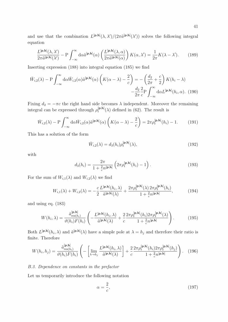
41

and use that the combination L[p,h](λ, λ′)/(2πa[p,h](λ′)) solves the following integral

equation

L[p,h](λ, λ′)

2πa[p,h](λ′)− P

ˆ ∞−∞

dαa[p,h](α)

(L[p,h](λ, α)

2πa[p,h](α)

)K(α, λ′) =

1

2πK(λ− λ′). (189)

Inserting expression (188) into integral equation (185) we find

Wi,2(λ)− P

ˆ ∞−∞

dαWi,2(α)a[p,h](α)

(K(α− λ)− 2

c

)= −

(d22π

+c

2

)K(hi − λ)

− d22π

2

cP

ˆ ∞−∞

dαL[p,h](hi, α). (190)

Fixing d2 = −πc the right hand side becomes λ independent. Moreover the remaining

integral can be expressed through ρ[p,h]t (λ) defined in (62). The result is

Wi,2(λ)− P

ˆ ∞−∞

dαWi,2(α)a[p,h](α)

(K(α− λ)− 2

c

)= 2πρ

[p,h]t (hi)− 1. (191)

This has a solution of the form

Wi,2(λ) = d3(hi)ρ[p,h]t (λ), (192)

with

d3(hi) =2π

1 + 2cn[p,h]

(2πρ

[p,h]t (hi)− 1

). (193)

For the sum of Wi,1(λ) and Wi,2(λ) we find

Wi,1(λ) +Wi,2(λ) = − c2

L[p,h](hi, λ)

a[p,h](λ)+

2πρ[p,h]t (λ) 2πρ

[p,h]t (hi)

1 + 2cn[p,h]

, (194)

and using eq. (183)

W (hi, λ) =a[p,h]res(hi)

ϑ(hi)F (hi)

(−L

[p,h](hi, λ)

a[p,h](λ)+

2

c

2πρ[p,h]t (hi)2πρ

[p,h]t (λ)

1 + 2cn[p,h]

). (195)

Both L[p,h](hi, λ) and a[p,h](λ) have a simple pole at λ = hj and therefore their ratio is

finite. Therefore

W (hi, hj) =a[p,h]res(hi)

ϑ(hi)F (hi)

(−[

limλ→hj

L[p,h](hi, λ)

a[p,h](λ)

]+

2

c

2πρ[p,h]t (hi)2πρ

[p,h]t (hj)

1 + 2cn[p,h]

). (196)

B.3. Dependence on constants in the prefactor

Let us temporarily introduce the following notation

α =2

c, (197)

42

β =α

1 + αn[p,h]. (198)

Combining the results of two previous subsections we obtain

Det(1− A) detmi,j=1 (δij +W (hi, hj)) =(1−K [p,h]

)β−1 det (Aij + βBij) , (199)

where we defined the following matrix elements

Aij = δij −a[p,h]res(hi)

ϑ(hi)F (hi)

[limλ→hj

L[p,h](hi, λ)

a[p,h](λ)

], (200)

Bij =a[p,h]res(hi)

ϑ(hi)F (hi)2πρ

[p,h]t (hi)2ρ

[p,h]t (hj). (201)

From the finite-size form factors [19] we know that the factor (199) is independent of α

and therefore also of β. Therefore choosing β = 1 we obtain

Det(1− A) detmi,j=1 (δij +W (hi, hj)) =(1−K [p,h]

)det (Aij +Bij) , (202)

Inserting expressions for Aij and Bij we get the final result reported in eq. (50).

It is interesting to try to prove that expression (199) is independent of β at the

thermodynamic level. For (199) to be independent of β, Aij must be of rank n− 1 and

Bij must be of rank 1 because then

det(Aij + βBij) = βdet(Aij +Bij). (203)

Matrix Bij has a product form and thus its rank is 1. It is more difficult to show that

the matrix Aij has rank n− 1. Consider the n = 1 case. Then we must have

a[p,h]res(h)

ϑ(h)F (h)limλ→h

L[p,h](h, λ)

a[p,h](λ)= 1. (204)

We have seen in [29] that this equality holds in the small momentum limit. Here, we

will show that it is also true for large c. We will keep the first two leading orders in 1/c.

The backflow function is

F (λ) = −p− hπc

(1 +

1

πc

ˆ ∞−∞

dαϑ(α) +O(1/c2)

). (205)

The a[p,h](λ) function is

a[p,h](λ) =ϑ(λ)

2π

p− λh− λ

(1 +

p− hπc

P

ˆ ∞∞

dαϑ(α)

α− λ+O(1/c2)

), (206)

and its residue is

a[p,h]res(h) = −ϑ(h)

2π(p− h)

(1 +

p− hπc

P

ˆ ∞∞

dαϑ(α)

α− h+O(1/c2)

). (207)

43

Therefore the right hand side is

ϑ(h)F (h)

a[p,h]res(h)

=2

c

(1 +

1

πc

ˆ ∞−∞

dαϑ(α)

)(1− p− h

πcP

ˆ ∞∞

dαϑ(α)

h− α

)−1=

2

c

(1 +

1

πcP

ˆ ∞−∞

dαϑ(α)

(1 +

p− hh− α

))=

2

c

(1 +

1

πcP

ˆ ∞−∞

dαϑ(α)p− αh− α

+O(1/c2)

). (208)

On the other hand the ratio L[p,h](λ, λ′)/a[p,h](λ′) is given by

L[p,h](λ, λ′)

a[p,h](λ′)=

2

c+

(2

c

)2

P

ˆ ∞−∞

dα a[p,h](α) +O(1/c3)

=2

c

(1 +

1

πcP

ˆ ∞−∞

dαϑ(α)p− αh− α

+O(1/c2)

). (209)

Therefore the identity holds for the first two orders in 1/c. We showed it also in the

small momentum limit of the two-particle form factors, see section 6.1. Proving that

eq. (199) is independent of β in full generality remains an open question.

B.4. Derivation of formula (125)

Comparing expressions for the form factors with 1 and m + 1 particle-hole excitations

we find

A(ϑ, {hj, pj}mj=0})A(ϑ, {h0, p0})

=A(ϑ, {hj, pj}mj=1})m∏j=1

[(p0 − hj + ic)2

(h0,j + ic)(p0,j + ic)

(pj − h0 + ic)2

(hj,0 + ic)(pj,0 + ic)

]1/2×

m∏j=1

h0,j p0,j(pj − h0)(p0 − hj)

. (210)

Let analyze first products involving the dominant excitation. For j = 1, . . . ,m we have

(p0 − hj + ic)2

(h0 − hj + ic)(p0 − pj + ic)=p0 − hj + ic

h0 − hj + ic. (211)

(pj − h0 + ic)2

(hj − h0 + ic)(pj − p0 + ic)=pj − h0 + ic

pj − p0 + ic. (212)

The product of these two terms is in the leading order a pure phase factor and its

contribution to the form factors can be neglected. To compute the correlation function

we need only the norm of the form factors. For i = 0 and j corresponding to a small

excitation we have(h0 − hj)(p0 − pj)(p0 − hj)(pj − h0)

= −1 +O(pj − hj). (213)

Therefore

A(ϑ, {hj, pj}mj=0}) =(−1)meiφA(ϑ, {hj, pj}mj=1})× (1 +O(pj − hj)) . (214)

44

We analyze now the term A(ϑ, {hj, pj}mj=1}) involving only small excitations. For

i, j = 1, . . . ,m we have

(pi − hj + ic)2

(hi − hj + ic)(pi − pj + ic)=

(hi − hj + ic+ pi − hi)(pi − pj + ic+ pj − hj)(hi − hj + ic)(pi − pj + ic)

= 1 +O(pj − hj). (215)

The double product, ∏mi<j=1(hi − hj)(pi − pj)∏m

i,j=1(pi − hj), (216)

remains as it is. Consider now the ratio of the back-flow functions. The back-flow

function is smooth, but the filling function is, for now, arbitrary. We have

πF0(pk) sinπF0(hk)

πF0(hk) sinπF0(pk)=ϑ(pk) sinπϑ(hk)F0(hk)

ϑ(hk) sinπϑ(pk)F0(hk). (217)

Finally ρt(λ) is a smooth function, irrespective of the filling function, and therefore can

be evaluated either at pi or hi. Putting all the pieces together we find

A(ϑ, {hj, pj}mj=0})A(ϑ, {h0, p0})

=

[m∏k=1

F0(hk)

ρt(hk)

ϑ(pk) sinπϑ(hk)F0(hk)

ϑ(hk) sinπϑ(pk)F0(hk)

] ∏mi<j=1(hi − hj)(pi − pj)∏m

i,j=1(pi − hj).

(218)

For the B(ϑ, {pj, hj}mj=0) term we find in the leading order O(pj − hj)

B(ϑ, {pj, hj}mj=0) = B (ϑ, {p0, h0}) +m∑k=1

P

ˆ +∞

−∞dλ

F (λ)(hk − pk)(λ− hk)(λ− pk)

. (219)

All the other terms in B(ϑ, {pj, hj}mj=0) that do not involve summation over excitations

depend, in the leading order, only on the backflow F0(λ) of the dominant excitation and

therefore are contained in B(ϑ, {p0, h0}). The remaining integral

ˆ +∞

−∞dλ

F (λ)(pk − hk)(λ− hk + ic)(λ− pk + ic)

, (220)

is proportional to pk − hk and therefore does not contribute to the leading order in

pk−hk. It might seem that the same is true for principal value integral. However, as we

will see later, the contribution of this integral depends on the smoothness of the filling

function ϑ(λ). As we do not require the filling function to be smooth everywhere, we

leave this term as it is.

The last piece is the D(ϑ, {pj, hj}mj=0) part. We have

D(ϑ, {pj, hj}mj=0)

D(ϑ, {p0, h0})=

detmi,j=0 (δij +W (hi, hj))

1 +W0(h0, h0)

Det(1− A)

Det(1− A0). (221)

45

Crucial in the evaluation of this ratio is function a[p,h](λ|{pj, hj}mj=0). Inspecting its form

we see that in the leading order in pk − hk its equal to the a[p,h](λ|{p0, h0}). Therefore

the ratio of the Fredholm determinants is equal to 1.

The remaining part involves matrix elements W (hi, hj) given in (51). The matrix

elements are proportional to a[p,h]res(hi)

which, for i = 1, . . . , n is of order pi− hi. Therefore

the leading order of the determinant is given by the contribution from the dominant

excitation and

D(ϑ, {pj, hj}mj=0)

D(ϑ, {p0, h0})= 1 +O(pj − hj). (222)

Combining the results for the three factors we find (125).

C. On the numerical evaluation of the Fredholm determinant

The new expression for the thermodynamic form factors (50) contains the Fredholm

determinant of the generalized resolvent. We restrict here to the single-particle case

Det(1 + L[p,h]). (223)

The numerical evaluation of the kernel L[p,h] is problematic due to the pole in λ′ = h.

The most straightforward way is to expand the determinant into traces, using the well

known formula

Det(1 + L[p,h]) = exp(Tr log(1 + L[p,h])

)= exp

(TrL[p,h] − 1

2Tr(L[p,h])2 +

1

3Tr(L[p,h])3 + . . .

), (224)

with

Tr(L[p,h])n =

ˆdλ1 . . . dλn−1L

[p,h](λ1, λ2) . . . L[p,h](λn−1, λ1). (225)

The principal value integrals can be computed using known relations

P

ˆ ∞−∞

dλf(λ)

h− λ= FT−1 ((iπsign(k)FT[f ]) (h), (226)

with the Fourier transform given by

FT(f) =

ˆ +∞

−∞dx eikxf(x), (227)

and the series (224) can be truncated with a small (odd) number of terms.

Another approach is to introduce a new kernel

L[p,h](λ, λ′) =L[p,h](λ, λ′)

h− λ′, (228)

46

and decompose L[p,h] as follows

L[p,h](λ, λ′) =

[L[p,h](λ, λ′)− L[p,h](λ, h)

h− λ′

]+L[p,h](λ, h)

h− λ′. (229)

The first kernel is regular in λ′ = h and therefore we denote it as L[p,h],reg

L[p,h](λ, λ′)− L[p,h](λ, h)

h− λ′= L[p,h],reg(λ, λ′). (230)

Using that L[p,h](λ,h)h−λ′ is a rank one matrix we obtain for the determinant (223)

Det(1+L[p,h]) = Det(1+L[p,h],reg)

(1 + P

ˆ ∞−∞

dλdλ′L[p,h](λ, h)

h− λ′[(1 + L[p,h],reg)−1](λ, λ′)

).

(231)

We use the usual resolvent technique to compute the inverse of the kernel (1 +

L[p,h],reg)−1 = 1− Sreg, which gives an integral equation for the kernel Sreg

Sreg(λ, λ′) +

ˆdαL[p,h],reg(λ, α)Sreg(α, λ′) = L[p,h],reg(λ, λ′). (232)

Finally we obtain

Det(1 + L[p,h]) = Det(1 + L[p,h],reg)

×

(1 + P

ˆ ∞−∞

dλL[p,h](λ, h)

h− λ−ˆ

dλP

ˆ ∞−∞

dλ′L[p,h](λ, h)

h− λ′S(λ, λ′)

).

(233)

The Fredholm determinant Det(1+L[p,h],reg) can be now easily evaluated with standard

numerical techniques [87]. For example by choosing a discretization λ → {xj}Ndj=1 and

computing the determinant of the finite size matrix (δij +N−1d L[p,h],reg(xi, xj)).