Embed Size (px)
Citation preview
SPIKING NEURON MODELS
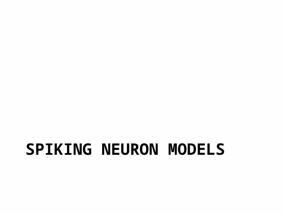
Spiking neuron models
Input =N spike trains
Output =1 spike train
A neuron model is defined by:• what happens when a spike is received• the condition for spiking• what happens when a spike is produced• what happens between spikes
discrete events
continuous dynamics
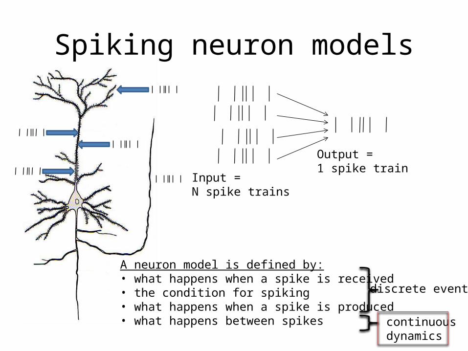
The membrane equation
Iinj
outside
inside
injLmm I
R
EV
dt
dVC
)(
=1/R
Vm
injmLm RIVEdt
dV RC membrane time constant
(typically 3-100 ms)

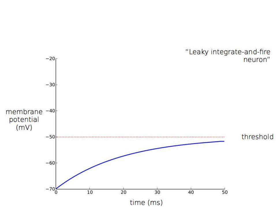
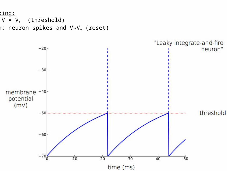
Spiking:If V = Vt (threshold)then: neuron spikes and V→Vr (reset)
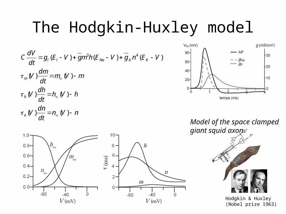
The Hodgkin-Huxley model
Hodgkin & Huxley(Nobel prize 1963)
nVndt
dnV
hVhdt
dhV
mVmdt
dmV
VEngVEhmgVEgdt
dVC
n
h
m
KKNall
)()(
)()(
)()(
)()()( 43
Model of the space clamped giant squid axon
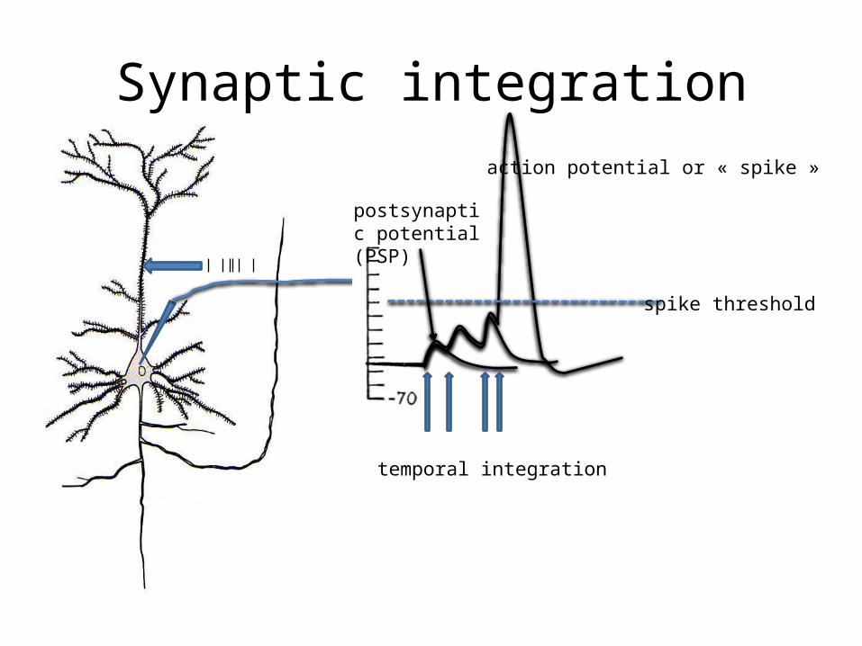
Synaptic integration
spike threshold
action potential or « spike »
postsynaptic potential (PSP)
temporal integration
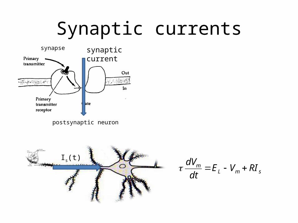
Synaptic currentssynaptic current
postsynaptic neuron
synapse
Is(t)
smLm RIVEdt
dV
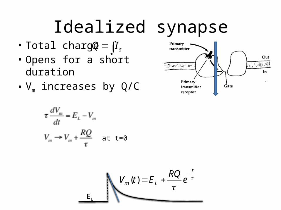
Idealized synapse• Total charge• Opens for a short duration• Vm increases by Q/C
sIQ
EL
t
Lm eRQ
EtV
)(
at t=0
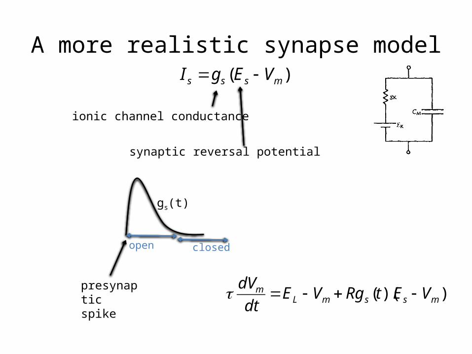
A more realistic synapse model)( msss VEgI
ionic channel conductance
synaptic reversal potential
gs(t)
presynaptic spike
open closed
))(( mssmLm VEtRgVEdt
dV
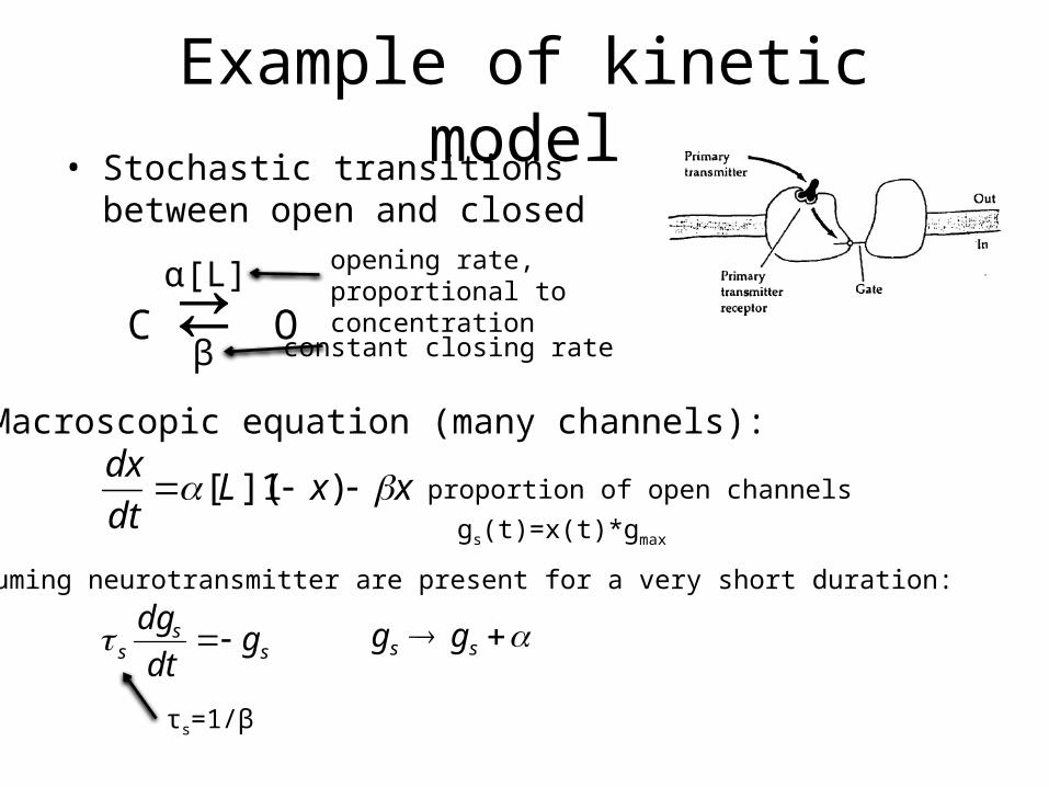
Example of kinetic model• Stochastic transitions between open
and closed
C ⇄ Oα[L]
βopening rate, proportional to concentration
constant closing rate
Macroscopic equation (many channels):
xxLdt
dx )1]([ proportion of open channels
Assuming neurotransmitter are present for a very short duration:
ss
s gdt
dg
τs=1/β
gs(t)=x(t)*gmax
ss gg
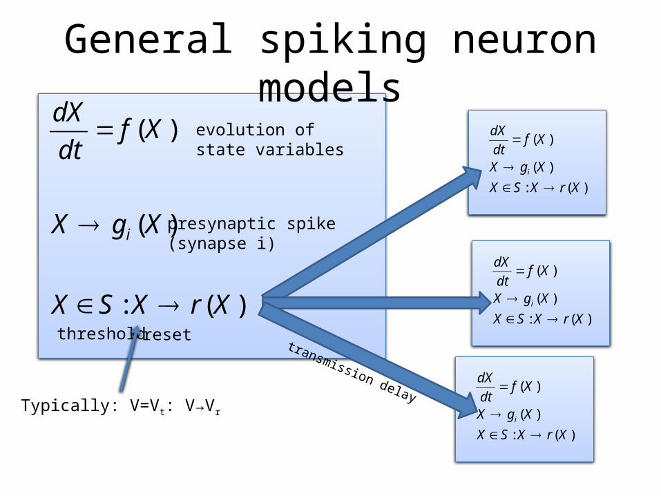
General spiking neuron models
)(:
)(
)(
XrXSX
XgX
Xfdt
dX
i
presynaptic spike(synapse i)
threshold reset
evolution of state variables
)(:
)(
)(
XrXSX
XgX
Xfdt
dX
i
)(:
)(
)(
XrXSX
XgX
Xfdt
dX
i
)(:
)(
)(
XrXSX
XgX
Xfdt
dX
i
transmission delayTypically: V=Vt: V→Vr

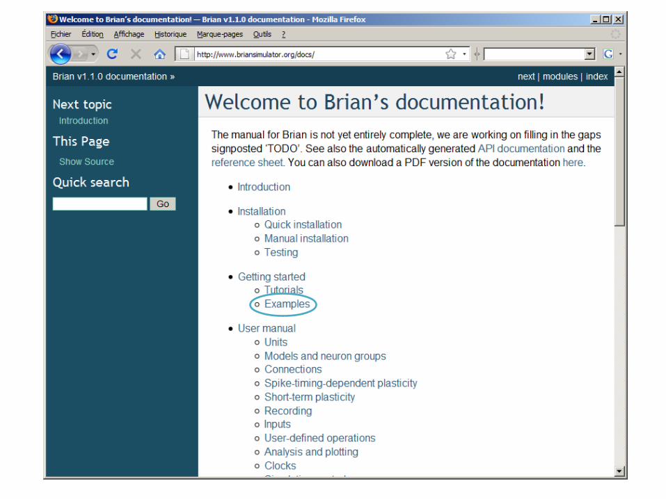
http://www.briansimulator.org
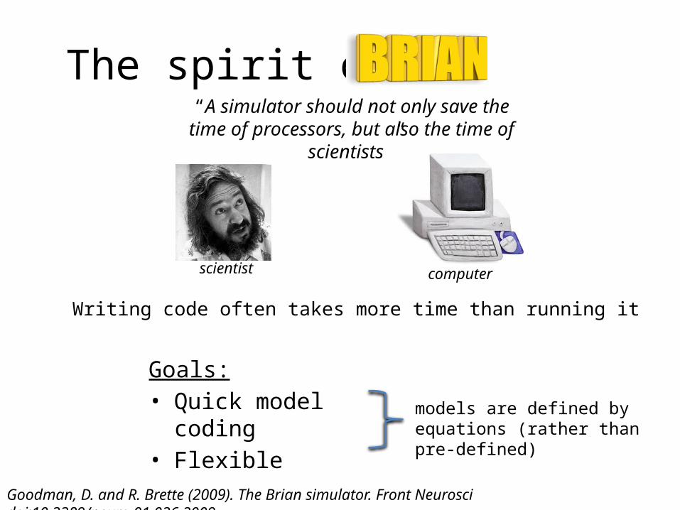
The spirit of “A simulator should not only save
the time of processors, but also the time of scientists”
scientist computer
Writing code often takes more time than running it
Goals:• Quick model coding• Flexible
models are defined by equations (rather than pre-defined)
Goodman, D. and R. Brette (2009). The Brian simulator. Front Neurosci doi:10.3389/neuro.01.026.2009.

Who is Brian?
briansimulator.org

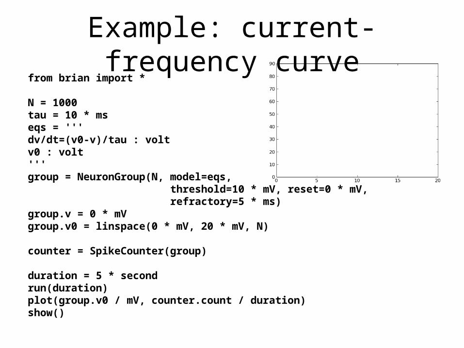
Example: current-frequency curvefrom brian import *
N = 1000tau = 10 * mseqs = '''dv/dt=(v0-v)/tau : voltv0 : volt'''group = NeuronGroup(N, model=eqs, threshold=10 * mV, reset=0 * mV, refractory=5 * ms)group.v = 0 * mVgroup.v0 = linspace(0 * mV, 20 * mV, N)
counter = SpikeCounter(group)
duration = 5 * secondrun(duration)plot(group.v0 / mV, counter.count / duration)show()
Example: a fully connected networkfrom brian import *
tau = 10 * msv0 = 11 * mVN = 20w = .1 * mV
group = NeuronGroup(N, model='dv/dt=(v0-v)/tau : volt', threshold=10 * mV, reset=0 * mV)
W = Connection(group, group, 'v', weight=w)
group.v = rand(N) * 10 * mV
S = SpikeMonitor(group)
run(300 * ms)
raster_plot(S)show()
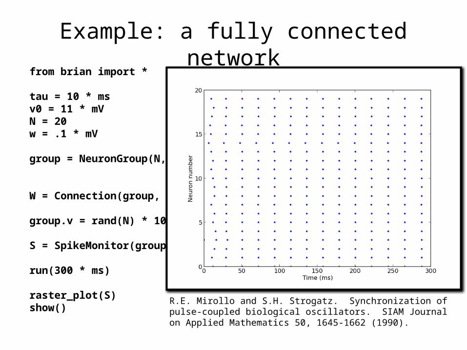
R.E. Mirollo and S.H. Strogatz. Synchronization of pulse-coupled biological oscillators. SIAM Journal on Applied Mathematics 50, 1645-1662 (1990).
Example 2: a ring of IF neuronsfrom brian import *
tau = 10 * msv0 = 11 * mVN = 20w = 1 * mV
ring = NeuronGroup(N, model='dv/dt=(v0-v)/tau : volt', threshold=10 * mV, reset=0 * mV)
W = Connection(ring, ring, 'v')for i in range(N): W[i, (i + 1) % N] = w
ring.v = rand(N) * 10 * mV
S = SpikeMonitor(ring)
run(300 * ms)
raster_plot(S)show()
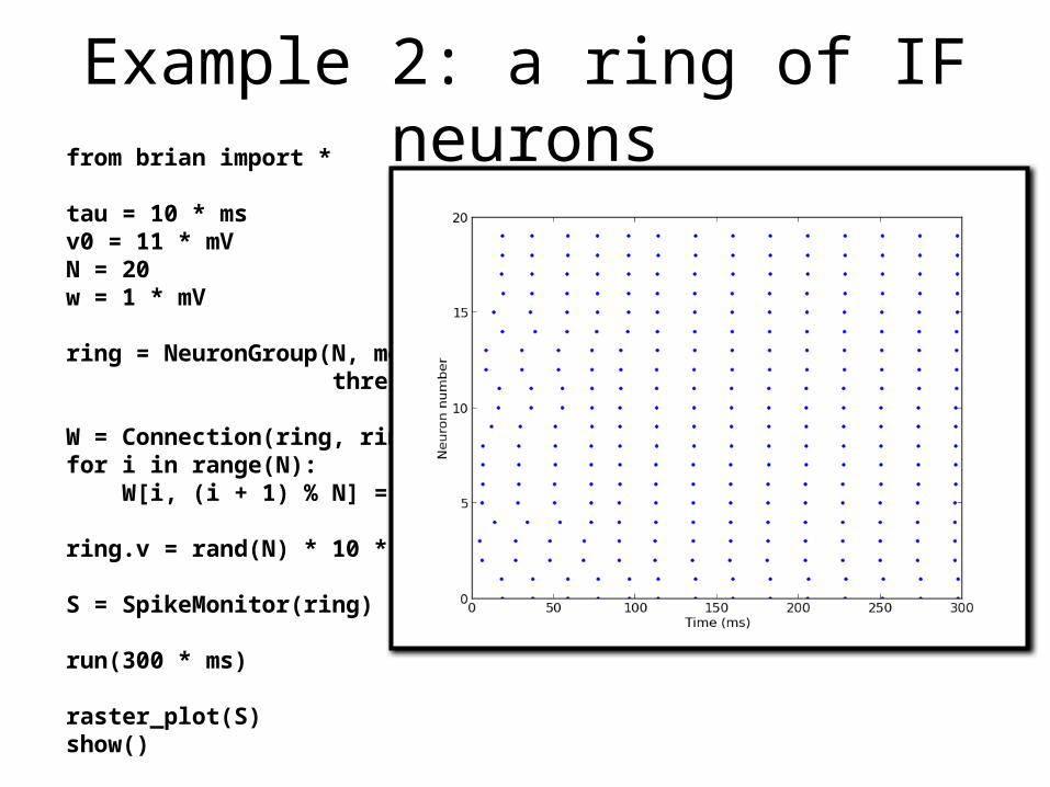
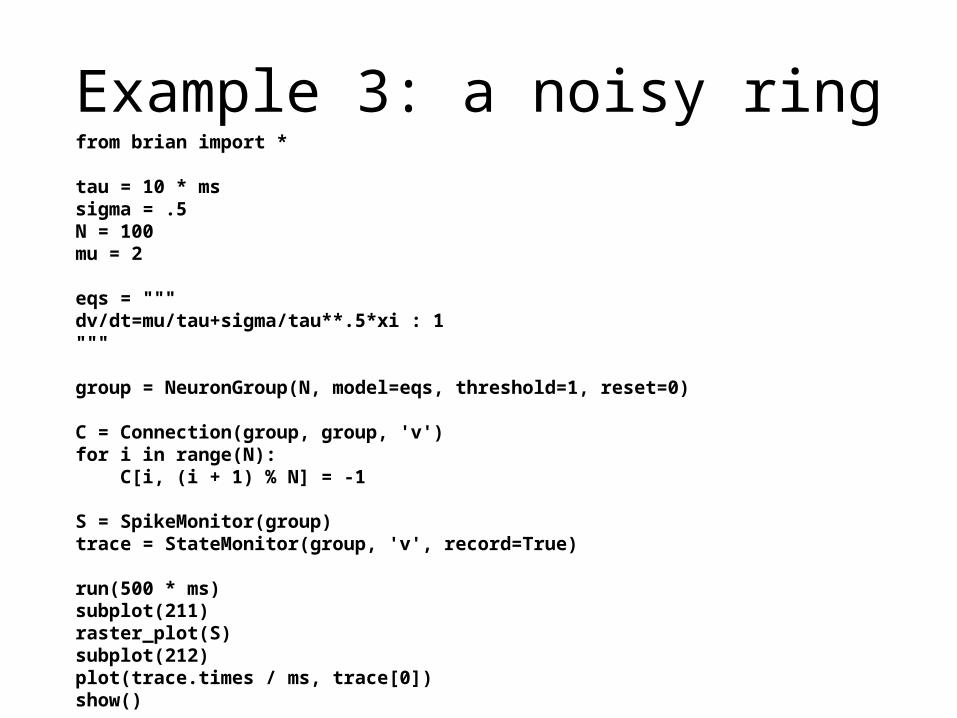
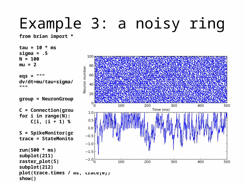
Example 3: a noisy ringfrom brian import *
tau = 10 * mssigma = .5N = 100mu = 2
eqs = """dv/dt=mu/tau+sigma/tau**.5*xi : 1"""
group = NeuronGroup(N, model=eqs, threshold=1, reset=0)
C = Connection(group, group, 'v')for i in range(N): C[i, (i + 1) % N] = -1
S = SpikeMonitor(group)trace = StateMonitor(group, 'v', record=True)
run(500 * ms)subplot(211)raster_plot(S)subplot(212)plot(trace.times / ms, trace[0])show()

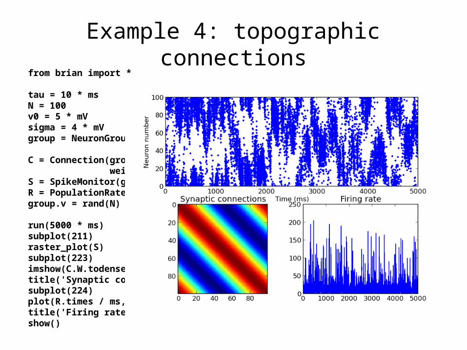
Example 4: topographic connectionsfrom brian import *
tau = 10 * msN = 100v0 = 5 * mVsigma = 4 * mVgroup = NeuronGroup(N, model='dv/dt=(v0-v)/tau + sigma*xi/tau**.5 : volt', threshold=10 * mV, reset=0 * mV)C = Connection(group, group, 'v', weight=lambda i, j:.4 * mV * cos(2. * pi * (i - j) * 1. / N))S = SpikeMonitor(group)R = PopulationRateMonitor(group)group.v = rand(N) * 10 * mV
run(5000 * ms)subplot(211)raster_plot(S)subplot(223)imshow(C.W.todense(), interpolation='nearest')title('Synaptic connections')subplot(224)plot(R.times / ms, R.smooth_rate(2 * ms, filter='flat'))title('Firing rate')show()
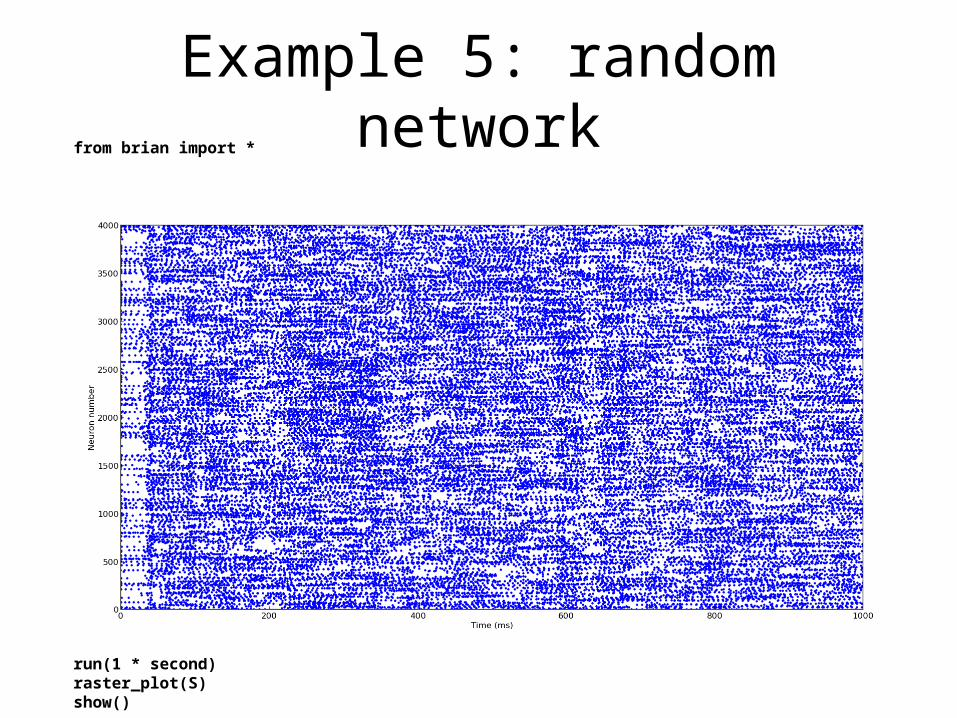
Example 5: random networkfrom brian import *
taum = 20 * msecondtaue = 5 * msecondtaui = 10 * msecondEe = 60 * mvoltEi = -80 * mvolt
eqs = '''dv/dt = (-v+ge*(Ee-v)+gi*(Ei-v))*(1./taum) : voltdge/dt = -ge/taue : 1dgi/dt = -gi/taui : 1'''
P = NeuronGroup(4000, model=eqs, threshold=10 * mvolt, reset=0 * mvolt, refractory=5 * msecond)Pe = P.subgroup(3200)Pi = P.subgroup(800)we = 0.6wi = 6.7Ce = Connection(Pe, P, 'ge', weight=we, sparseness=0.02)Ci = Connection(Pi, P, 'gi', weight=wi, sparseness=0.02)P.v = (randn(len(P)) * 5 - 5) * mvoltP.ge = randn(len(P)) * 1.5 + 4P.gi = randn(len(P)) * 12 + 20
S = SpikeMonitor(P)
run(1 * second)raster_plot(S)show()
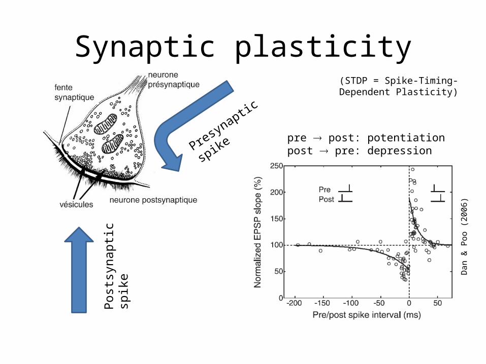
Synaptic plasticity
Presynaptic spike
Post
syna
ptic
spik
e
Dan
& P
oo (2
006)
pre post: potentiation post pre: depression
(STDP = Spike-Timing-Dependent Plasticity)
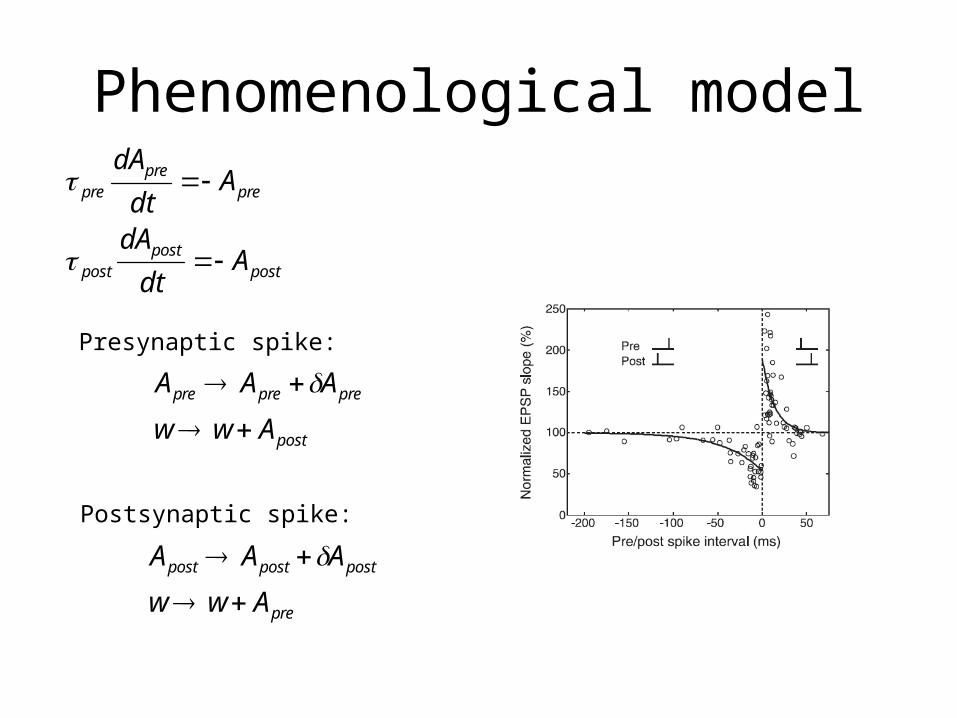
Phenomenological model
postpost
post
prepre
pre
Adt
dA
Adt
dA
Presynaptic spike:
post
preprepre
Aww
AAA
Postsynaptic spike:
pre
postpostpost
Aww
AAA
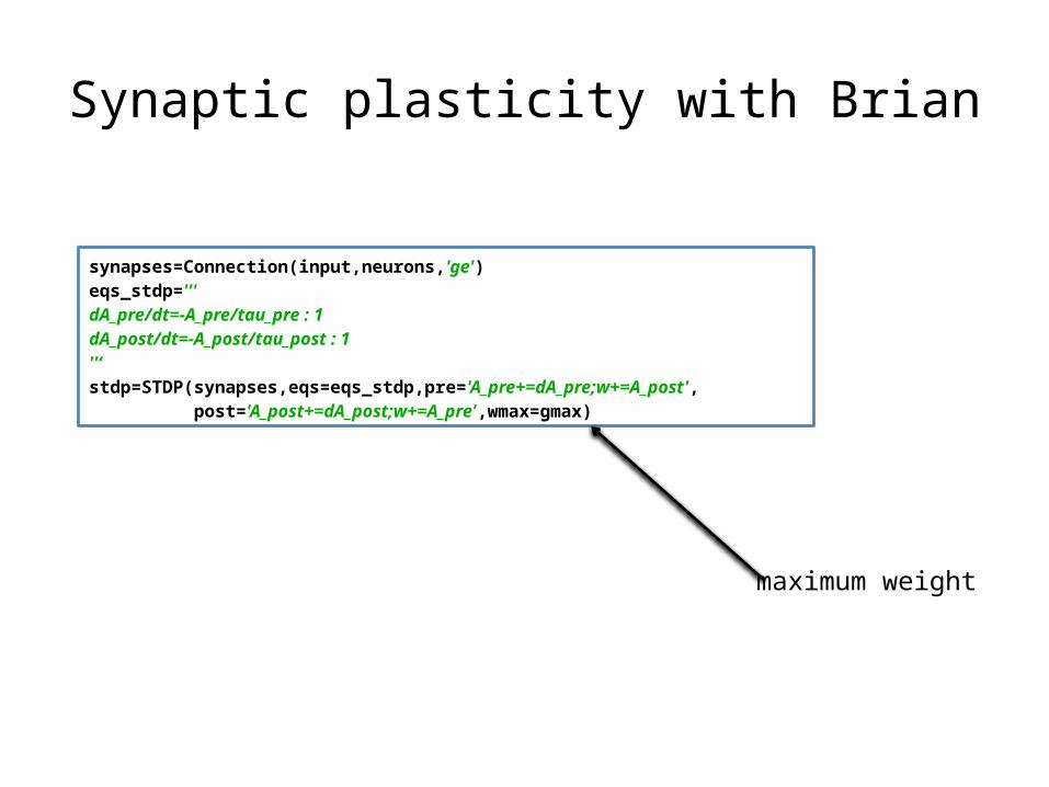
Synaptic plasticity with Brian
synapses=Connection(input,neurons,'ge') eqs_stdp='''dA_pre/dt=-A_pre/tau_pre : 1dA_post/dt=-A_post/tau_post : 1''‘stdp=STDP(synapses,eqs=eqs_stdp,pre='A_pre+=dA_pre;w+=A_post', post='A_post+=dA_post;w+=A_pre',wmax=gmax)
maximum weight
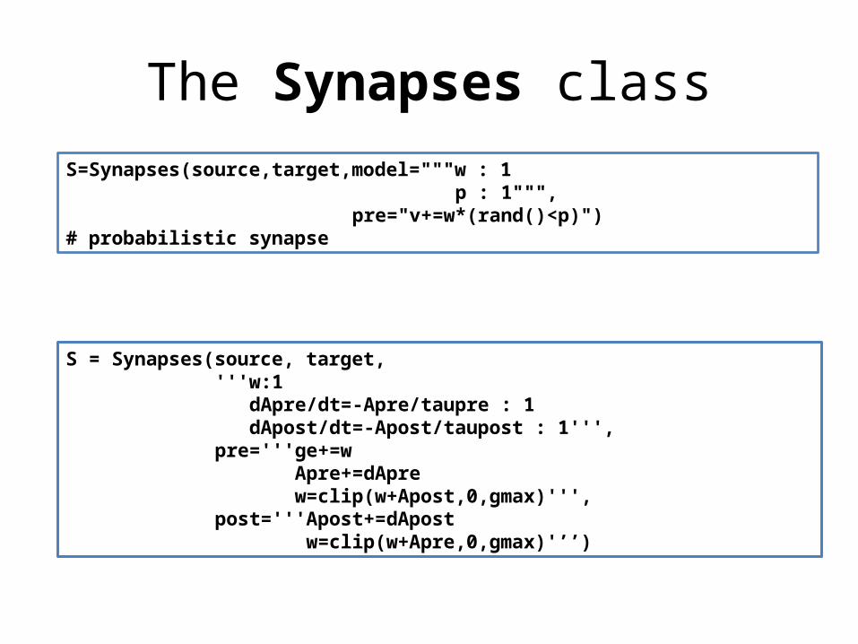
The Synapses classS=Synapses(source,target,model="""w : 1 p : 1""", pre="v+=w*(rand()<p)")# probabilistic synapse
S = Synapses(source, target, '''w:1 dApre/dt=-Apre/taupre : 1 dApost/dt=-Apost/taupost : 1''', pre='''ge+=w Apre+=dApre w=clip(w+Apost,0,gmax)''', post='''Apost+=dApost w=clip(w+Apre,0,gmax)'’’)

https://github.com/brian-team/brian2http://brian2.readthedocs.org

What’s new with ?
• More flexibility• Code is generated for targets
Python C++ Android Anything else
Achilles Koutsou
BrianDROID
Thanks
Bertrand Fontaine Cyrille Rossant
Dan Goodman
Victor Benichoux
Marcel Stimberg
http://www.briansimulator.org